A Numerical Method for Computing the Jordan Canonical Form
Zhonggang Zeng and Tien-Yien Li
A numerical method for computing the Jordan Canonical Form
Abstract
The Jordan Canonical Form of a matrix is highly sensitive to perturbations, and its numerical computation remains a formidable challenge. This paper presents a regularization theory that establishes a well-posed least squares problem of finding the nearest staircase decomposition in the matrix bundle of the highest codimension. A two-staged algorithm is developed for computing the numerical Jordan Canonical Form. At the first stage, the method calculates the Jordan structure of the matrix and an initial approximation to the multiple eigenvalues. The staircase decomposition is then constructed by an iterative algorithm at the second stage. As a result, the numerical Jordan Canonical decomposition along with multiple eigenvalues can be computed with high accuracy even if the underlying matrix is perturbed.
keywords Jordan canonical form, eigenvalue, staircase form,
1 Introduction
This paper presents an algorithm and a regularization theory for computing the Jordan Canonical Form accurately even if the matrix is perturbed.
The existence of the Jordan Canonical Form is one of the fundamental theorems in linear algebra as an indispensable tool in matrix theory and beyond. In practical applications, however, it is well documented that the Jordan Canonical Form is extremely difficult, if not impossible, for numerical computation [3, p.25], [5, p.52], [8, p.189], [9, p.165], [13, p.146], [23, p.371], [26, p.132], [44, p.22]. In short, as remarked in a celebrated survey article by Moler and Van Loan [38]: “The difficulty is that the JCF cannot be computed using floating point arithmetic. A single rounding error may cause some multiple eigenvalue to become distinct or vise versa, altering the entire structure of and .”
Indeed, defective multiple eigenvalues in a non-trivial Jordan Canonical Form degrade to clusters of simple eigenvalues in practical numerical computation. A main theme of the early attempts for numerical computation of the Jordan Canonical Form is to locate a multiple eigenvalue as the mean of a cluster that is selected from eigenvalues computed by QR algorithm and, when it succeeds, the Jordan structure may be determined by computing a staircase form at the multiple eigenvalue. This approach includes works of Kublanovskaya [33] (1966), Ruhe [41] (1970), Sdridhar et al [43] (1973), and culminated in Golub and Wilkinson’s review [24] (1976) as well as Kågström and Ruhe’s JNF [29, 30] (1980). Theoretical issues have been analyzed in, e.g. [11, 12, 48, 49].
However, the absence of a reliable method for identifying the proper cluster renders a major difficulty for this approach. Even if the correct cluster can be identified, its arithmetic mean may not be sufficiently accurate for identifying the Jordan structure, as shown in Example 1 (§4). While improvements have been made steadily [6, 37], a qualitative approach is proposed in [8], and a partial canonical form computation is studied in [31], “attempts to compute the Jordan canonical form of a matrix have not been very successful” as commented by Stewart in [44, p. 22].
A related development is to find a well-conditioned matrix such that is block diagonal [23, §7.6.3]. Gu proved this approach is NP-hard [25], with a suggestion that “it is still possible that there are algorithms that can solve most practical cases” for the problem. Another closely related problem is the computation of the Kronecker Canonical Form for a matrix pencil (see [15, 16, 17, 28]). For a given Jordan structure, a minimization method is proposed in [36] to find the nearest matrix with the same Jordan structure.
Multiple eigenvalues are multiple roots of the characteristic polynomial of the underlying matrix. There is a perceived barrier of “attainable accuracy” associated with multiple zeros of algebraic equations which, in terms of number of digits, is the larger one between data error and machine precision divided by the multiplicity [39, 50, 53]. Thus, as mentioned above, accurate computation of multiple eigenvalues remains a major obstacle of computing the Jordan Canonical Form using floating point arithmetic. Recently, a substantial progress has been achieved in computing multiple roots of polynomials. An algorithm is developed in [53] along with a software package [52] that consistently determines multiple roots and their multiplicity structures of a polynomial with remarkable accuracy without using multiprecision arithmetic even if the polynomial is perturbed. The method and results realized Kahan’s observation in 1972 that multiple roots are well behaved under perturbation when the multiplicity structure is preserved [32].
Similar to the methodology in [53], we propose a two-stage algorithm in this paper for computing the numerical Jordan Canonical Form. To begin, we first find the Jordan structure in terms of the Segre/Weyr characteristics at each distinct eigenvalue. With this structure as a constraint, the problem of computing the Jordan Canonical Form is reformulated as a least squares problem. We then iteratively determine the accurate eigenvalues and a staircase decomposition, and the Jordan decomposition can follow as an option.
We must emphasize the numerical aspect of our algorithm that focuses on computing the numerical Jordan Canonical Form of inexact matrices. The exact Jordan Canonical Form of a matrix with exact data may be obtainable in many cases using symbolic computation (see, e.g. [10, 21, 22, 35]). Due to ill-posedness of the Jordan Canonical Form, however, symbolic computation may not be suitable for applications where matrices will most likely be perturbed in practice. For those applications, we must formulate the notion of the numerical Jordan Canonical Form that is structurally invariant under small data perturbation, and continuous in a neighborhood of the matrix with the exact Jordan Canonical Form in question.
More precisely, matrices sharing a particular Jordan structure form a matrix bundle, or, a manifold. For a given matrix , we compute the exact Jordan Canonical Form of the nearest matrix in a bundle of the highest co-dimension within a neighborhood of . Under this formulation, computing the numerical Jordan Canonical Form of should be a well-posed problem when is sufficiently close to bundle . In other words, under perturbation of sufficiently small magnitudes, the deviation of the numerical Jordan Canonical Form is tiny with the structure intact.
The main results of this paper can be summarized as follows. In §3, we formulate a system of quadratic equations that uniquely determines a local staircase decomposition at a multiple eigenvalue from a given Jordan structure. Regularity theorems (Theorem 1 and Theorem 2) in this section establish the well-posedness of the staircase decomposition that ensures accurate computation of multiple eigenvalues. Based on this regularity, the numerical unitary-staircase eigentriplets is formulated in §4, along with the backward error measurement and a proposed condition number.
In §5, we present an iterative algorithm for computing the well-posed unitary-staircase eigentriplet assuming the Jordan structure is given. The algorithm employs the Gauss-Newton iteration whose local convergence is a result of the regularity theorems given in §3. The method itself can be used as a stand-alone algorithm for calculating the nearest staircase/Jordan decomposition of a given structure, as demonstrated via numerical examples in §5.4.
The algorithm in §5 requires a priori knowledge of the Jordan structure, which can be computed by an algorithm we propose in §6. The algorithm employs a special purpose Hessenberg reduction and a rank-revealing mechanism that produces the sequence of minimal polynomials. Critically important in our algorithm is the application of the recently established robust multiple root algorithm [53] to those numerically computed minimal polynomials in determining the Jordan structure as well as an initial approximation of the multiple eigenvalues, providing the crucial input items needed in the staircase algorithm in §5. In §7, we summarize the overall algorithm and present numerical results
2 Preliminaries
2.1 Notation and terminology
Throughout this paper, matrices are denoted by upper case letters , , etc., and denotes a zero matrix with known dimensions. Vectors are in columns and represented by lower case boldface letters like , and . A zero vector is denoted by , or to emphasize the dimension. The notation represents the transpose of a matrix or a vector , and is its Hermitian adjoint (or conjugate transpose). The fields of real and complex numbers are denoted by and respectively.
For any matrix , the rank, nullity, range and kernel of are denoted by , , and respectively. The identity matrix is , or simply when its size is clear. The column vectors of are canonical vectors . A matrix is said to be unitary if . A matrix is called a unitary complement of unitary matrix if is a square unitary matrix. Subspaces of n are denoted by calligraphic letters , , with dimensions , , etc., and stands for the orthogonal complement of subspace . The set of distinct eigenvalues of is the spectrum of and is denoted by .
2.2 Segre and Weyr characteristics
The Jordan structure and the corresponding staircase structure (see §2.3) of an eigenvalue can be characterized by the Segre characteristic and the Weyr characteristic respectively. These two characteristics are conjugate partitions of the algebraic multiplicity of the underlying eigenvalue. Here, a sequence of nonnegative integers is called a partition of a positive integer if . For such a partition, sequence , is called the conjugate partition of . For example, is a partition of with conjugate and vice versa.
Let be an eigenvalue of with an algebraic multiplicity corresponding to elementary Jordan blocks of orders . The infinite sequence is called the Segre characteristic of associated with . The Segre characteristic forms a partition of the algebraic multiplicity of . Its conjugate partition is called the Weyr characteristic of associated with . We also take the Weyr characteristic as an infinite sequence for convenience. The nonzero part of such sequences will be called the nonzero Segre/Weyr characteristics. Let be an matrix with Weyr characteristic associated with an eigenvalue . Then [14, Definition 3.6 and Lemma 3.2], for ,
which immediately implies the uniqueness of the two characteristics and their invariance under unitary similarity transformations, since the rank of is the same as the rank of for . In particular, both characteristics are invariant under Hessenberg reduction [23, §7.4.3].
2.3 The staircase form
Discovered by Kublanovskaya [33], a matrix is associated with a staircase form given below.
Lemma 1
Let be a matrix with nonzero Weyr characteristic associated with an -fold eigenvalue . For consecutive , let be a matrix satisfying . Then is of full rank and
| (1) | |||||
| (13) |
Furthermore, all super-diagonal blocks are matrices of full rank.
Proof. Equation (1) and the existence of in (13) can be proved by a straightforward verfication using for . From (13), we have
This implies is of full rank since with will lead to , contradicting to the linear independence of columns of .
The matrix in (1) is called a local staircase form of associated with . The matrix is called a staircase nilpotent matrix associated with eigenvalue . Writing , we call the array as in (1) a staircase eigentriplet of associated with Weyr characteristic . It is called unitary-staircase eigentriplet of if is a unitary matrix. The unitary-staircase form is often preferable to Jordan Canonical Form itself since the columns of in (1) form an orthonormal basis for the invariant subspace of associated with .
Let . Lemma 1 lead to the existence of a unitary matrix satisfying [24, 33, 41]
| (14) |
The matrix in (14) is called a staircase form of and the matrix factoring is called a unitary-staircase decomposition of . A staircase decomposition of matrix can be converted to Jordan decomposition via a series of similarity transformations [24, 30, 33, 41].
2.4 The notion of the numerical Jordan Canonical Form
Corresponding to a fixed set of integer partitions for with , the collection of all matrices with distinct eigenvalues associated with Segre characteristics for forms a manifold, known as a matrix bundle originated by A. I. Arnold [1]. This bundle has a codimension that can be represented in terms of Segre/Wyre characteristics [1, 14]
| (15) |
where for are corresponding Weyr characteristics. When a matrix belongs to such a bundle, it can also be in the closure of many bundles with respect to different Segre characteristics. In other words, a matrix with certain Jordan structure can be arbitrarily close to matrices with other Jordan structures. For example, matrix deformations
| (16) |
show that a matrix with Segre characteristic is arbitrarily close to some matrices with Segre characteristic , which are arbitrarily near certain matrices with Segre characteristic . Let denote the matrix bundle with respect to the Segre characteristics listed in and denote its closure. Then (16) suggests that and . Extensively studied in e.g. [7, 14, 16, 17, 20], these closure relationships form a hierarchy or stratification of Jordan structures that can be conveniently decoded by a covering relationship theorem by Edelman, Elmroth and Kågström [17, Theorem 2.6]. As an example, Figure 1 lists all the Jordan structures and their closure stratification for matrices in different Segre characteristics and codimensions of matrix bundles.

Let present the distance of a matrix to a bundle . When is near a bundle , say listed in Figure 1, then clearly since . Indeed, matrix is automatically as close, or even closer, to ten other bundles of lower codimensions below following the hierarchy. In practical applications and numerical computation, the given matrix comes with imperfect data and/or roundoff error. We must assume with a perturbation of small magnitude on the original matrix . The main theme of this article is: How to compute the Jordan Canonical Form of the matrix accurately from its inexact data .
Suppose matrix has an exact nontrivial Jordan Canonical Form and thus belongs to a bundle of codimension , then there is a lower bound for the distance from to any other bundle of codimension . When is the given data of with an imperfect accuracy, that is, with a perturbation , then generically resides in the bundle of codimension 0. As a result, the Jordan structure of is lost in exact computation on for its (exact) Jordan Canonical Form. However, the original bundle where belongs to has a distinct feature: it is of the highest codimension among all the bundles passing through the -neighborhood of , as long as satisfies . Therefore, to recover the desired Jordan structure of from its empirical data , we first identify the matrix bundle of the highest codimension in the neighborhood of , followed by determining the matrix on that is closest to . The numerical Jordan Canonical Form of will then be defined as the exact Jordan Canonical Form of . In summary, the notion of the numerical Jordan Canonical Form is formulated according to the following three principles:
-
•
Backward nearness: The numerical Jordan Canonical Form of is the exact Jordan Canonical Form of certain matrix within a given distance , namely .
-
•
Maximum codimension: Among all matrix bundles having distance less than of , matrix lies in the bundle with the highest codimension.
-
•
Minimum distance: Matrix is closest to among all matrices in the bundle .
Definition 1
For and , let be the matrix bundle such that
and satisfying with (exact) Jordan decomposition . Then is called the numerical Jordan Canonical Form of within , and is called the numerical Jordan decomposition of within .
Remark: The same three principles have been successfully applied to formulate other ill-posed problems with well-posed numerical solutions such as numerical multiple roots [53] and numerical polynomial GCD [51, 54]. In this section, we shall attempt to determine the structure of the bundle with the highest codimension in the neighborhood of . The iterative algorithm EigentripletRefine developed in §5.2 is essentially used to find the matrix in the bundle which is nearest to matrix .
There is an inherent difficulty in computing the Jordan structure from inexact data and/or using floating point arithmetic. If, for instance, a matrix is near several bundles of the same codimension with almost identical distances, then the structure identification may not be a well determined problem. Therefore, occasional failures [18] for computing the numerical Jordan Canonical Form can not be completely eliminated.
3 Regularity of a staircase eigentriplet
For an eigenvalue of matrix with a fixed Weyr characteristic, the components and of the staircase eigentriplet in the staircase decomposition are not unique. We shall impose additional constraints for achieving uniqueness which is important in establishing the well-posedness of computing the numerical staircase form.
Theorem 1
Let and of multiplicity with nonzero Weyr characteristic . Then for almost all there is a unitary matrix and a staircase nilpotent matrix as in (13) such that
| (19) | |||||
| where | (20) | ||||
| and | (21) | ||||
Moreover, if there is another unitary matrix and a staircase nilpotent matrix that can substitute and in (19), then where for a diagonal matrix with .
The second equation in (19) along with the index set in (20) means that, for , the matrix is lower triangular where and . For example: Let be an eigenvalue with Weyr characteristic , we have multiplicity , , and , , , , , , , , , . The matrix has zero at every entry. As shown in Figure 2, those zeros are under the staircase and above the diagonal.
Proof of Theorem 1. For , the subspace is of dimension . For almost all vectors , , the subspace
is of dimension one and spanned by a unit vector which is unique up to a unit constant multiple. After obtaining , the subspace
is of dimension one and spanned by which is again unique up to a unit constant multiple. Therefore, we have a unitary matrix , whose columns satisfy the second equation in (19) and span the subspace for . These unitary matrices uniquely determines in (13). It is straightforward to verify (19) for .
One of the main components of our algorithm is an iterative refinement of the eigentriplet using the Gauss-Newton iteration. For this purpose we need to construct a system of analytic equations for the eigentriplet specified in Theorem 1. If the matrix and the eigenvalue are real, it is straightforward to set up the system using equations in along with the orthogonality equaiton . When either matrix or eigenvalue is complex, however, the unitary constraint is not analytic. One way to circumvent this difficulty is converting (19) and to real equations by splitting and the eigentriplet into real and imaginary parts. The resulting system of real equations would be real analytic.
Alternatively, we developed a simple and effective strategy to overcome this difficulty by a two step approach. As an initial approximation, a staircase eigentriplet is computed and does not need to be unitary. We replace the unitary constraint with a nonsingularity requirement
| (22) |
via a constant matrix . The solution to the equation (22) combined with (19) is a nonsingular matrix whose columns span the invariant subspace of associated with . Then, at the second step, can be stably orthogonalized to and provide the solution of (19). If necessary, we repeat the process as refinement by replacing with in (22) along with (19) and solve for again using the previous eigentriplet results as the initial iterate. In the spirit of Kahan’s well-regarded “twice is enough” observation [40, p. 110], this reorthogonalization never needs the third run.
In general, let be the set of predetermined random complex vectors as in Theorem 1. A second set of complex vectors will also be chosen to set up the overdetermined quadratic system
| (23) |
where is defined in (20). There are equations and unknowns in (23) where
| (24) |
with a difference . Let
| (25) |
where is the Kronecker delta, and denote vectors of components and respectively, ordered by the rule where precedes if , or with . The unknowns in eigentriplet are ordered in a vector form
| (26) |
where is the column vector consists of the entries of in the order illustrated in the following example for the Weyr characteristic :
| (33) | |||||
With this arrangement, the Jacobian of is an matrix.
Theorem 2
Let be an -fold eigenvalue of associated with nonzero Weyr characteristic . Then for almost all vectors , there is a unique pair of matrices and where is a staircase nilpotent matrix in the form of (13) such that the staircase eigentriplet satisfies the system (23). Moreover, the Jacobian of in (25) is of full column rank at .
Proof. The subspace is of dimension for . For each , the subspace is of dimension one and spanned by the unique vector with . Theirfore vectors are uniquely defined so that for where , . Moreover, and for . It is straightforward to verify for being a nilpotent staircase matrix in the form of (13) with uniquely determined blocks
Consequently, the matrix pair satisfying (23) exists and is unique for almost all .
We now prove the Jacobian of in (25) is of full rank at a staircase eigentriplet . The Jacobian can be considered a linear transformation which maps into ζ, where , and is a nilpotent staircase matrix of relative to the nonzero Weyr characteristic . We partition with blocks in the same way as we partition in (13) for . Assume is rank-deficient. Then there is a triplet such that , namely
| (34) | |||||
| (35) | |||||
| (36) |
Using and for , we have
| (37) |
from (34). A simple induction using (37) leads to , for . Namely, vectors all belong to the invariant subspace of associated with , and thus holds for certain .
Also by a straightforward induction we have
| (38) |
We claim that
| (39) |
This is true for because of (37). Assume (39) is true for . Then by (38)
since, again, for . Thus (39) holds for .
Since, , hence from . From (39), we have , By Lemma 1, is of full rank. Consequently, by (39), namely for . Therefore, for every , is in
for , implying . The equation (34) them implies and thus since is of full column rank. Consequently, is of full column rank.
The component in the staircase eigentriplet satisfying (23) is a unitary matrix for a particular . This will be achieved in our eigentriplet refinement process.
4 The numerical staircase eigentriplet and its sensitivity
Consider an complex matrix along with a fixed partition of integer (multiplicity) . Let the vector function be defined defined in (25) with respect to fixed vectors and and is its Jacobian. An array is called a numerical unitary-staircase eigentriplet of with respect to nonzero Weyr characteristic if satisfies , a necessary condition for to reach a local minimum at . The requirement can be satisfied in our refinement algorithm that is to be elaborated in §5.2.
If possesses a numerical unitary-staircase eigentriplet with a small residual
| (40) |
then, letting be a unitary complement of , it is straightforward to verify that
| (41) |
possesses as its exact unitary-staircase eigentriplet and the distance
is small. We now derive the well-posedness and the sensitivity measurement in a heuristic manner. Let be an -fold numerical unitary-staircase eigentriplet of with residual for defined in (25) via certain auxiliary vectors and . To analyze the effect of perturbation on matrix , let denote the same vector function in (25) where is now considered as a variable. When becomes by adding a matrix of small norm, denote as a numerical unitary eigentriplet of . Let us estimate the asymptotic bound of error
where and denote the vector forms of and respectively according to the rule given in (26). Write . Since is the local minimum in a neighborhood of , we have
for small and . Moreover,
In other words,
where is the Jacobian of and represents the higher order terms of . Let be the smallest singular value of matrix . Then is strictly positive by Theorem 2 and
where represents the higher order terms of . This provides an asymptotic bound
| (42) |
and the finite positive real number
| (43) |
serves as a condition number of the unitary-staircase eigentriplet that measures its sensitivity with respect to perturbations on matrix .
Definition 2
Let be a numerical unitary-staircase eigentriplet of as a regular orthogonal solution to the system corresponding to auxiliary vectors and in (25). Let be the Jacobian of . Then we call the staircase condition number for the eigentriplet.
Remark. The arithmetic mean of an eigenvalue cluster is often used as an approximation to a multiple eigenvalue. Let be an -fold eigenvalue of with an orthonormal basis matrix for the invariant subspace. The perturbed matrix has a cluster of eigenvalues around . Chatelin [9, pp.155–156] established the bound on the arithmetic mean as
| (44) |
for small , where is a matrix whose columns form a basis for the invariant subspace of . We call the cluster condition number of . From our computing experiments, the cluster condition number can be substantially larger than the staircase condition number as shown in the following example.
Example 1
Matrix
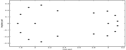
has two exact eigenvalues and with Segre characteristics and respectively. Under round-off perturbation in the magnitude of machine precision (), Matlab outputs eigenvalues in two noticeable clusters show in Figure 3. The arithmetic means of the two clusters are as follows
                        means                exact eigenvalues    cluster condition number
        left cluster:   1.99724665369002     2.000000000000000         6.50e+012
        right cluster:  3.00275334630999     3.000000000000000         6.48e+012
From these results, we can see that only 3 correct digits are obtained by grouping. In contrast, our iterative method, which will be presented in §5, converges on the two eigentriplets accurately and attains 14 correct digits on the two eigenvalues.
          Computed eigenvalues             2.00000000000004     3.00000000000003
          ---------------------------------------------------------------------------
          forward error                    4.00e-15             3.02e-14
          backward error                   1.65e-17             5.77e-17
          staircase condition number       3.45e+07             5.33e+05
The cluster condition numbers are over and the staircase condition numbers are substantially smaller ( and ). From the examples we have tested, computing staircase eigentriplet appears to be always more accurate than grouping clusters.
5 Computing a staircase eigentriplet with a known structure
In this section we present the method for computing a numerical unitary-staircase eigentriplet under the assumption that the Weyr characteristic is known for an -fold eigenvalue that is approximated by . An algorithm for computing the required Weyr characteristic and initial approximations to the eigenvalues will be given in the next section (§6). There are two steps in calculating the staircase eigentriplet : First find an initial staircase eigentriplet , then the Gauss-Newton iteration is applied to refine the eigentriplet until a desired accuracy is attained.
The QR decomposition and its updating/downdating will be used extensively. When a row is deleted from a matrix to form a new matrix , finding a QR decomposition of from an existing QR decomposition of is called a QR downdating. Conversely, computing the QR decomposition after inserting a row called a QR updating. QR updating and downdating are standard techniques in matrix computation [23, §12.5.3] requiring flops.
5.1 Computing the initial staircase eigentriplet
When is available with known multiplicity and nonzero Weyr characteristic , we need an initial approximation to the solution of equations (19). Write with . From the uniqueness in Theorem 1, each column of along with the -th column of is the unique solution to the homogeneous system
| (45) |
up to a unit multiple for and where is as in (13). Consequently, the vector consists of components , spans the one-dimensional kernel of the matrix
| (46) |
Let be the QR decomposition of . Then the vector can be computed by a simple inverse iteration [34] on
| (47) |
After is computed from , the next vector will be computed from which comes from deleting from the top row of and inserting at the bottom. Namely, the QR decomposition of is obtained from that of via a QR updating and a QR downdating.
In summary, computing the initial staircase eigentriplet is a process consisting of repeated QR updating/downdating and consecutive applications of inverse iteration (47), as outlined in the following pseudo-code.
-
Algorithm InitialEigentriplet
-
Input: matrix , Weyr char. , initial eigenvalue
-
–
get random vectors and QR decomposition of
-
–
for do
-
-
–
-
Output ,
Remark: Computing a staircase form from a given eigenvalue was proposed by Kublanovskaya [33] in 1968. Ruhe [41] improved the Kublanovskaya Algorithm in 1970 by employing singular value decomposition (SVD) for determining the numerical rank and kernel. Due to successive SVD computation, the original Kublanovskaya-Ruhe approach leads to an algorithm [6] in the worst case senerio. Further improvement has been proposed in [6, 24] that reduce the complexity to . Our Algorithm InitialEigentriplet can be considered a new improvement from Kublanovskaya-Ruhe Algorithm. The novelty of our algorithm includes (a) the nullity-one homogeneous system (45); (b) employing an efficient null-vector finder (47) to replace the costly SVD; and (c) successive QR updating/downdating. As a result, Algorithm InitialEigentriplet is of complexity and fits our specific need in satisfying the second constraint in (19). Furthermore, our computation of staircase form goes further with a refinement step using the Gauss-Newton iteration in the following section.
5.2 Iterative refinement for a staircase eigentriplet
The initial eigentriplet produced by Algorithm InitialEigentriplet (or by existing variations of the Kublanovskaya Algorithm) may not be accurate enough. One of the main features of our algorithm is an iterative refinement strategy for ensuring the highest achievable accuracy in computing the staircase eigentriplet. We elaborate the process in the following.
Since approximately satisfies (45), this eigentriplet is an approximate solution to (23) for . Using these ’s in (23) and (25), we apply the Gauss-Newton iteration for ,
| (48) |
with initial iterate . Here again, denotes the vector form of according to the rule given in (26).
Let be a least squares solution of with sufficiently small residual, or equivalently is close to a matrix having as its exact eigentriplet. Then the Jacobian is injective by Theorem 2, ensuring the Gauss-Newton iteration (48) to converges to locally. This is a numerical staircase eigentriplet, a unitary-staircase eigentriplet can be obtained by an orthogonalization and an extra step of refinement. Specifically, Let be the “economic” QR decomposition with . Partitioning the same way as , it is straightforward to verify that for if has as an exact eigenvalue with Weyr characteristic , and is the corresponding nilpotent staircase form. Furthermore, by resetting , , , , the equations in (23) are satisfied including the auxilliary equations.
In actual computation with the empirical data matrix , a small error may emerge during the reorthogonalization process. This error can easily be eliminated by one extra step of refinement via the Gauss-Newton iteration starting from the new eigentriplet .
-
Algorithm EigentripletRefine
-
Input: Initial approximate unitary-staircase eigentriplet , tolerance
-
–
Set , and
-
–
For do
-
-
–
Economic QR decomposition and set
-
–
If , exit. Otherwise, set , reset and , and repeat the algorithm
-
–
-
Output
To carry out the iterative refinement (48), a QR decomposition is required at every iteration step. A straightforward QR decomposition costs flops, which can be substantially reduced by taking the structure of the Jacobian into account. Using the Weyr characteristic as an example, the nilpotent staircase matrix is shown in (33). the Jacobian of with a re-arrangement of columns and rows and becomes
where the blocks for . Without loss of generality, we can assume is in Hessenberg form. Then is near triangular and requires only flops for its QR decomposition. The backward substitution requires flops.
5.3 Converting a staircase form to Jordan decomposition
After finding a staircase decomposition , the Jordan Canonical Form of is available by conjugating the Weyr characteristic. In the cases where the Jordan decomposition is in demand, a method for converting the staircase decomposition to the Jordan decomposition is proposed by Kublanovskaya [33] which primarily involves non-unitary similarity transformations. Detailed procedures can also be found in [24, 30].
Alternatively, we may calculate the Jordan decomposition by converting unitary-staircase eigentriplets to Jordan decompositions for using Kublanovskaya’s algorithm.
5.4 Numerical examples for computing the staircase form
Algorithm InitialEigentriplet combined with Algorithm EigentripletRefine forms a stand-alone algorithm for computing a staircase/Jordan decomposition, assuming an initial approximation to a multiple eigenvalue together with its Segre/Weyr characteristics are available by other means. This combination is implemented as a Matlab module EigTrip. We shall present a method for computing the Jordan structure in §6.
A previous algorithm for computing a staircase form with known Segre characteristic via a minimization process is constructed by Lippert and Edelman [36] and implemented as a Matlab module sgmin. The iteration implemented in sgmin converges in many cases, including difficult test matrices such as the Frank matrix. As we shall show below, our algorithm provides a substantial improvement over sgmin particularly on cases where the cluster condition numbers (44) are large but the staircase condition numbers stay moderate. We list the comparisons on accuracy only.
Example 1
’ We test both sgmin and our EigTrip on the matrix given in Example 1 in §4, starting from eigenvalue approximation and with given Segre characteristics and respectively. The code sgmin improves the eigenvalue accuracy by one and four digits respectively. In contrast, our EigTrip obtains an accuracy near the machine precision on both eigenvalues, as shown in Table 1.
| from | from | |||
| computed | backward | computed | backward | |
| eigenvalue | error | eigenvalue | error | |
| cluster mean | 1.99724665369002 | — | 3.00275334630999 | — |
| sgmin | 1.99991878946447 | 1.004e-008 | 2.99999991118127 | 6.895e-010 |
| EigTrip | 1.99999999999998 | 3.270e-017 | 3.000000000000003 | 4.673e-017 |
Example 2
We construct a matrix having known multiple eigenvalues and with Segre characteristics , and respectively, together with ten simple eigenvalues randomly generated in the box . Both sgmin and EigTrip start at initial approximations , , and . The results of the iterations are listed in Table 2, in which forward errors are for each computed eigenvalue , , and the backward errors are the residual (40) for each eigentriplet.
| at | at | at | ||||
|---|---|---|---|---|---|---|
| forward | backward | forward | backward | forward | backward | |
| error | error | error | error | error | error | |
| sgmin | 2.29e-008 | 8.46e-007 | 5.01e-008 | 9.42e-007 | 1.03e-009 | 3.15e-008 |
| EigTrip | 2.22e-016 | 1.16e-015 | 0 | 1.89e-016 | 8.88e-016 | 1.23e-016 |
The results show that our algorithm is capable of calculating eigenvalues to the accuracy near machine precision (16 digits). For each approximate eigentriplet of matrix , the residual is defined in (40). By (4), with relative distance up to from , there is a nearby matrix for which is an exact eigentriplet.
Example 3
(Frank matrix) [8, 24, 30, 37, 41, 45, 47]: This is a classical test matrix given in a Hessenberg form , with for and otherwise. Frank matrix has no multiple eigenvalues. However, its small eigenvalues are ill-conditioned measured by the standard eigenvalue condition number [23], as shown in the following table.
| Eigenvalues and condition numbers of Frank matrix | |||||
| Eigenvalue | condition | Eigenvalue | condition | Eigenvalue | condition |
| 32.22889 | 8.5 | 3.51186 | 34.1 | 0.143647 | 611065747.8 |
| 20.19899 | 16.2 | 1.55399 | 1512.5 | 0.081228 | 2377632497.8 |
| 12.31108 | 9.0 | 0.64351 | 1371441.3 | 0.049507 | 3418376227.8 |
| 6.96153 | 24.1 | 0.28475 | 53007100.5 | 0.031028 | 1600156877.4 |
Clearly, Frank matrix is near matrices which possess multiple eigenvalues near zero with nontrivial Jordan structures. Using an initial eigenvalue estimation near zero and Segre characteristics , , , and in consecutive tests, our refinement algorithm EigTrip produces five nearby matrices with an eigenvalue of multiplicity 2, 3, 4, 5, and 6 respectively, as shown in the table below.
| 5 nearby matrices with following features respectively | |||||
| given | computed | backward | staircase | cluster | |
| Segre ch. | eigenvalue | error | condition | condition | |
| sgmin | {6} | 0.1870511240986754 | 6.34e-05 | 126.8 | |
| EigTrip | {6} | 0.1870509025041315 | 6.34e-05 | 5.96 | |
| sgmin | {5} | 0.1076751260727581 | 1.90e-06 | 7689.2 | |
| EigTrip | {5} | 0.1076751114381528 | 1.90e-06 | 32.2 | |
| sgmin | {4} | 0.0701182985767899 | 6.12e-08 | 291589.8 | |
| EigTrip | {4} | 0.0703019426541069 | 3.47e-08 | 447.4 | |
| sgmin | {3} | 0.0504328996330119 | 4.23e-l0 | 3666804.6 | |
| EigTrip | {3} | 0.0504338685708545 | 4.23e-10 | 11322.9 | |
| sgmin | {2} | 0.0305042120283680 | 9.87e-10 | 15192435.2 | |
| EigTrip | {2} | 0.0386493437615946 | 3.45e-12 | 458607.1 | |
In other words, Frank matrix resides within a relative distance from a matrix having a double eigenvalue, or from a matrix having a triple eigenvalue, etc. Notice that the cluster condition numbers (44) in both cases are quite high whereas the staircase condition numbers are small. It appears that our Algorithm EigTrip substantially improves backward accuracy over sgmin, particularly when cluster condition number is large.
6 Computing the numerical Jordan structure
In this section we present the theory and algorithm for computing the structure of the numerical Jordan Canonical Form represented by Segre and Weyr characteristics.
6.1 The minimal polynomial
As described in many textbooks on fundamental algebra (see, e.g. [2]), given a linear operator on a vector space over a field , one may view as a module over by a “scalar” product: for and . For , , and being the matrix representation of , we consider n a module over the polynomial ring with scalar product for and .
A monic polynomial is called an annihilating polynomial for (with respect to ) if . For a subspace , if for all , then is regarded as an annihilating polynomial for . The polynomial with least degree among all the annihilating polynomials for (or subspace ) is called the minimal polynomial for (or subspace ). Note that every annihilating polynomial for (or subspace ) is divisible by the minimal polynomial and obviously the minimal polynomial for subspace is divisible by any minimal polynomial for any vector in . If the minimal polynomial for a vector coincides with the minimal polynomial for then is said to be a regular vector of .
By the Fundamental Structure Theorem for modules over Euclidean domain [2], n is a direct sum of cyclic submodules, say , where for each , is a cyclic submodule (a submodule spanned by one vector) invariant with respect to and is isomorphic to with being the minimal polynomial for . Moreover, each is divisible by for , that is . Here, for polynomial and , notation stands for “ divides ”.
It follows from that each for can be written in the form
| (49) |
for fixed , and for .
Lemma 2
When a subspace is invariant with respect to , the linear transformation induces a linear map given by . All the concepts and statements on annihilating polynomials and minimal polynomials introduced above for n with linear map can be repeated for with linear map . For instance, is the minimal polynomial for subspace if is the least degree polynomial which annihilates all , that is for all .
When is isomorphic to a vector space over with isomorphism , then the linear map induces a linear map , making the diagram in Figure 4 commutes. That is, .
Lemma 3
For any subspace , is the minimal polynomial for with respect to if and only if is the minimal polynomial of with respect to .
Proof. implies for any integer . It follows that for any . Thus for and
| (50) |
Let be the minimal polynomial for (with respect to ) and be the minimal polynomial for (with respect to ). Then, by (50), implies for all . So, annihilates and hence . By the same argument , and the assertion follows.
6.2 The Jordan structure via minimal polynomials
By Lemma 2, the first task in finding the Jordan structure of is to identify the minimal polynomial for the corresponding cyclic submodules , in , followed by factorizing in the form given in (49). We must emphasize here that accurate factorization of in numerical computation used to be regarded as a difficult problem. However, the appearance of a newly developed numerical algorithm MultRoot [52, 53] for calculating multiple roots and their multiplicities makes this problem well-posed and solvable. Consequently the structure of the Jordan Canonical Form can be determined accurately.
We shall begin by finding the minimal polynomial for . From , every can be written in the form where for . Thus, by , we have , making the minimal polynomial for n. Meanwhile, is the minimal polynomial for all except those ’s for which . The exceptional set is of measure zero. Therefore almost every is a regular vector. In other words, vector is regular with probability one if it is chosen at random as in §6.3.
To find minimal polynomial , we choose a generic vector and check the dimensions of the Krylov subspaces , , , consecutively to look for the first integer where is of dimension . For this , let . Obviously, and
can serve as the minimal polynomial of . We then proceed to find the minimal polynomial for . By the same argument given above along with the property , is the minimal polynomial for (by as well as the minimal polynomial for almost all . By Lemma 3, is the minimal polynomial for (with respect to the induced linear map ), and, with probability one, the minimal polynomial for any vector in . To derive the induced map , let be an orthonormal basis for . Then forms a basis for n, and by writing for any vector , forms a basis for . For the matrix representation of , let
| (51) | |||||
with . It follows that
and the matrix
becomes the matrix representation of the linear transformation with respect to the basis . Meanwhile, by (51), , for . With the matrix representation of available, we may find the minimal polynomial for (with respect to ) by following the same procedure that produces minimal polynomial for (with respect to ). For instance, using generically chosen , write and consider (). Checking the sequence of Krylov subspaces , , consecutively. Let be the first one with its dimension less than the number of generating vectors. That is, the relation with exists, and polynomial becomes the minimal polynomial for . With probability one, it is the minimal polynomial for (with respect to ). Therefore .
Notice that the linear independence of in implies the linear independence of in n. Thus and . In general, , for , so the same process may be continued to find the minimal polynomial for , .
6.3 The minimal polynomial via Hessenberg reduction
In the process elaborated in the last section (§6.2), a crucial step for finding minimal polynomials is the determination of the dimensions of the Krylov subspaces spanned by vector sets for . However, the condition of the Krylov matrix deteriorates when increases, making the rank decision difficult. A more reliable method is developed below to decide the dimension of accurately without the explicit calculation of the Krylov matrices.
Computing eigenvalues of a matrix starts with the Hessenberg reduction [23, p.344]
| (52) |
Let be the column vectors of in (52). Then
Here . Clearly, is an upper triangular matrix. Therefore
| (53) |
is a QR decomposition of the Krylov matrix . Furthermore, if is of full rank, then the first columns of form an orthonormal basis for the Krylov subspace .
Taking (53) into account for computing the minimal polynomial via Krylov matrices for using randomly chosen unit vector , the Hessenberg reduction matrix in (52) must have as its first column. This can be achieved by a modified Hessenberg reduction
| (54) |
Since , the first column of is the same as . The subsequent Hessenberg reduction steps of with unitary transformations does not change its first columns. Consequently the first -column block of stay the same for with . Upon completing (54) for up to , we obtain the Hessenberg matrix with a specified first column in .
When the Krylov matrix is of full rank, then and . Thus, the rank of can be decided by finding the numerical rank of during the process (54). Moreover, implies where are columns of . Consequently
Therefore, the numerical rank of is the same as the upper-triangular matrix . We summarize this result in the following proposition.
Proposition 3
For , let be the unitary transformation matrix whose first column is parallel to such that is upper-Hessenberg. Assume is the smallest integer for which Krylov matrix is rank-deficient, then for .
When Krylov matrices for are of full rank, the matrix is rank-deficient in exact sense if and only if the diagonal entry is zero since the matrix is upper-triangular. In numerical computation, however, an upper-triangular matrix can be numerically rank deficient even though its diagonal entries are not noticeably small, e.g., the Kahan matrix [23, p.260]. That is, is usually small but not near zero for to be numerically rank deficient. Therefore we must apply the inverse iteration (47) to determine whether is rank deficient in approximate sense.
When the first index is encountered with being numerically rank-deficient, we can further refine the Hessenberg reduction and minimize the magnitude of the entry of since
| (55) |
should be zero, here is the first -entry subvector of for . As a result, the least squares solution to the overdetermined system
| (56) |
minimizes . Here is the predetermined random vector and are constant vectors. Let be the vector mapping that represents the left side of the system (56) and be its Jacobian. The following proposition ensures the local convergence of the Gauss-Newton iteration in solving for the least squares solution.
Proposition 4
Proof. Differentiating the system (56), let matrix and upper-Hessenberg matrix satisfy
| (57) |
Using an induction, we have and assume . The equation becomes . For , we have from , , for . Also, and lead to and since . Thus and for . Namely, is injective.
When is numerically rank-deficient, we set and the initial iterate for the Gauss-Newton iteration
that refines the (partial) Hessenberg reduction and minimize the magnitude of the residual that approaches zero during the iterative refinement.
Overwrite with the terminating iterate of (6.3) and be the QR decomposition of . Then
with being an upper-Hessenberg matrix whose characteristic polynomial is the first minimal polynomial of . By the argument in § 6.2, the second minimal polynomial of is the (first) minimal polynomial of . Therefore we can continue the same Hessenberg reduction-refinement strategy on recursively and obtain a reduced-Hessenberg form
| (59) |
where each is an irreducible upper-Hessenberg matrix whose characteristic polynomial is the -th minimial polynomial of for .
The first minimal polynomial and its coefficient vector satisfies . From (53), , and being full rank, we have where is a upper triangular matrix and
In general, to find the coefficient vector of the -th minimal polynomial for , we first solve for and write
Then solve
| (61) |
-
Algorithm MinimalPolynomials
-
Input: , numerical rank threshold
-
–
Initialize
-
–
While do
-
-
–
-
Output: minimal polynomials
The sequence of minimal polynomials , , produced by Algorithm MinimalPolynomials are in the form
where is the Segre characteristic of associated with for . Although the process is recursive, there is practically no loss of accuracy from to since is extracted as a submatrix of during which only unitary similarity transformations are involved.
For each , Algorithm MultRoot in [52, 53] is applied to calculate the multiplicity structure and corresponding approximate roots , obtaining the Jordan structure of matrix .
Remark. The modified Hessenberg reduction (54) is in fact the Arnoldi process [42, p. 172-179] with Householder orthogonalization, which is the most reliable version of the Arnoldi method. We improve its robustness even further with a novel iterative refinement step (6.3). There are less reliable versions of the Arnoldi iteration (see, e.g. [13, p.303][23, p.499]) based on Gram-Schmidt orthogonalization that may be applied to construct unitary bases for the Krylov subspaces. A method of finding minimal polynomials can alternatively be based on those versions of the Arnoldi algorithm. We choose the modified Hessenberg reduction and Gauss-Newton refinement to ensure the highest possible accuracy.
6.4 Minimal polynomials and matrix bundle stratification
In fact, the process of applying Algorithm MinimalDegree on matrix sequence , , inherently calculates the Segre characteristics associated with the matrix bundle of the highest codimension. Suppose belongs to matrix bundle defined by Segre characteristics , for . As explained in §2.4, bundle is imbedded in the closure of a lower codimension matrix bundle, say , in a hierarchy of bundle stratification. Our algorithm actually identifies the highest codimension bundle because of the covering relationship established in [17].
For minimal polynomials of , let for . The integer sequence forms a partition of . Let be the similarly constructed sequence of minimal polynomial degrees associated with bundle where .
Lemma 4
Suppose and are two bundles of matrices with and a matrix on has at least as many distinct eigenvalues as a matrix on . Let and be the degree sequences of minimal polynomials associated with and respectively. Then and as partitions of satisfy the dominant ordering relationship , namely
| (62) |
Proof. By [17, Theorem 2.6], if and only if it is possible to coalesce eigenvalues and apply the dominance ordering coin moves to the Segre characteristics which defines bundle to reach those of . If is obtained by one dominance coin move from one Segre characteristic to with other Segre characteristics unchanged, then and therefore (62) holds.
Similarly, assume is obtained by coalescing two eigenvalues on with their Wyre characteristics combined as a union of sets, or equivalently, their Segre characteristics and combined in a componentwise sum and other Segre characteristics unchanged (see also [17, Lemma 2.5]). Actually the equalities in (62) hold in this case since the degree is the sum of the -th components in the Segre characteristics.
Since (62) is valid for every single dominant coin move and every coalesce of eigenvalues, it holds for a sequence of such manipulations of Segre characteristics from to .
Because of (62), we have either or . If , there is an such that and . Algorithm MinimalDegree applying on stops at instead of , since the search goes through degree 1, 2, and precedes . Consequently, the highest codimension bundle is identified before with proper rank calculation. If , the degrees of minimal polynomials associated with is the same as those of . For a similar reason, Algorithm MultRoot [52] extracts the highest codimension multiplicity structure that leads to rather than . Consequently, the highest codimension bundle is identified before with proper rank calculation. Our computing experiment is consistent with this observation.
7 The overall algorithm and numerical results
7.1 The overall algorithm
Our overall algorithm for computing the numerical Jordan Canonical Form of given matrix can now be summarized as follows.
-
Stage I: Computing the Jordan Structure
-
Step 1 Francis QR. Apply Francis QR algorithm to obtain a Schur decomposition and approximate eigenvalues .
-
Step 2 Deflation. For each well-conditioned simple eigenvalue , apply the deflation method in [4] to swap downward along the diagonal of to reach
where consists of all the well-conditioned eigenvalues of .
-
Step 3 Jordan structure. Apply the method in §6.3 to calculate the Segre characteristics of and initial estimates of the distinct eigenvalues.
-
-
Stage II: Computing the staircase/Jordan decompositions
There is an option here to select either the unitary staircase decompsition or the Jordan decomposition .-
Step 4(a) To compute the staircase decomposition. For each distinct eigenvalue, apply Algorithm InitialEigentriplet for an initial eigentriplet using the Segre characteristic and initial eigenvalue approximation computed in the previous step. Then iteratively refine the eigentriplet by Algorithm EigentripletRefine. Continue this process to reach a unitary staircase decomposition ultimately.
-
Step 4(b) To compute the Jordan decomposition. For each distinct eigenvalue , with Segre characteristic and the initial approximate determined in Step 3 above, apply the precess described in §5 to compute a unitary-staircase eigentriplet . Then apply the Kublanovskaya algorithm to obtain the local Jordan decomposition . Consequently, the Jordan decomposition with is constructed.
-
As mentioned before, Stage II can be considered a stand-alone algorithm for computing the staircase/Jordan form from given Weyr/Segre characteristics and initial eigenvalue approximation. It can be used in conjunction with other approaches where the Jordan structure is determined by alternative means.
There are four control parameters that can be adjusted to improve the results:
-
1.
The deflation threshold : If a simple eigenvalue has a condition number less than , it will be deflated. The default value for is .
-
2.
The gap threshold in rank decision : In determining the rank deficiency of in Algorithm MinimalDegree, we calculate the smallest singular value of each . If the ratio of the smallest singular values of and is less than , then is considered rank deficient. The default value for is .
-
3.
The residual tolerance for MultRoot: The residual tolerance required by MultRoot. See [53] for details.
-
4.
The residual tolerance for eigentriplet refinement: It is used to stop the iteration in refining the eigentriplet. The default value .
7.2 Numerical results
We made a Matlab implementation NumJCF of our algorithm for computing the Jordan decomposition. It has been tested in comparison with the Matlab version of JNF [29] on a large number of matrices, including classical examples in the literature. Our experiment is carried out on a Dell Optiplex GX 270 personal computer with Intel Pentium 4 CPU, 2.66 GHz and 1.5 GB RAM. For a computed Jordan decomposition of matrix , the residual is used as one of the measures for the accuracy
Example 4
Let
We compare our method with the conventional symbolic computation on the exact matrix. The exact eigenvalues are , and with Segre characteristics , and , respectively. For , and , it takes Maple 10 nearly two hours (7172 seconds) to find the Jordan Canonical Form, while both JNF and NumJCF complete the computation instantly. On a similarly constructed matrix of size , Maple does not finish the computation in 8 hours and Mathematica runs out of memory.
| computed eigenvalues | residual | |||
|---|---|---|---|---|
| (with correct digits in boldface and Jordan block sizes in braces) | ||||
| JNF | 1.414213563 {1} | 1.732050809 {2} | 2.236067975 {3} | 3.38e-013 |
| NumJCF | 1.41421356237311 {1} | 1.732050807574 {2} | 2.23606797749971 {3} | 1.01e-016 |
Approximating and in machine precision , both JNF and NumJCF correctly identify the Jordan structure, whereas our NumJCF obtained the eigenvalues with more correct digits than JNF along with smaller residual as shown in Table 3.
Example 5
| Computing results for eigentriplets of | |||
| eigenvalue | Segre characteristic | residual | |
| 1.0000000000000002 | {1, 0} | ||
| JNF | 2.0000000000000001 | {3, 2} | 1.41e-15 |
| 3.0000000000000002 | {2, 2} | ||
| 0.9999999999999995 | {1, 0} | ||
| NumJCF | 2.0000000000000000 | {3, 2} | 1.40e-16 |
| 3.0000000000000003 | {2, 2} | ||
Both JNF and NumJCF obtain similarly accurate results on classical matrices such as those in [8, pp. 192-196]. We choose to omit them and concentrate on the cases in which our NumJCF significantly improves the robustness and accuracy in comparison with JNF.
Example 6
This is a series of test matrices with a parameter .
| (63) |
For every , matrix has the same Jordan Canonical Form consisting of two eigenvalues and with Segre characteristics and respectively. Let the Jordan decomposition be . When increases, the condition number of increases rapidly. This example tests the accuracy and robustness of numerical Jordan Canonical Form finders under the increasing condition number of . As shown in Table 4, our algorithm maintains high backward accuracy, forward accuracy, and structure correctness, while the results of JNF deteriorate as increases. Starting from , JNF outputs incorrect Jordan structure. When , JNF outputs only one Jordan block. Our NumJCF continues to produce accurate results.
| eigenvalues | Segre ch. | backward error | |||
| 2.00000000000001 | 3,1 | ||||
| JNF | 2.99999999999999 | 4,2 | 6.10e-015 | ||
| 2.00000000000000 | 3,1 | 1113.9 | |||
| NumJCF | 3.00000000000000 | 4,2 | 1.11e-015 | ||
| 2.000000000002 | 3,1 | ||||
| JNF | 2.999999999998 | 4,2 | 7.40e-014 | ||
| 2.00000000000000 | 3,1 | 28894.5 | |||
| NumJCF | 3.00000000000000 | 4,2 | 4.87e-016 | ||
| 1.99999999987 | 3,1 | ||||
| JNF | 3.00000000009 | 4,2 | 8.30e-012 | ||
| 2.00000000000000 | 3,1 | 1658396.6 | |||
| NumJCF | 2.99999999999999 | 4,2 | 5.65e-016 | ||
| 2.0000000006 | 4 | ||||
| JNF | 2.9999999996 | 5,1 | 1.36e-011 | ||
| 2.00000000000001 | 3,1 | 5655648.5 | |||
| NumJCF | 2.99999999999999 | 4,2 | 7.60e-016 | ||
| 2.0000001 | 4 | ||||
| JNF | 2.99999992 | 5,1 | 9.29e-010 | ||
| 2.00000000000003 | 3,1 | 297244917.4 | |||
| NumJCF | 2.99999999999998 | 4,2 | 6.94e-016 | ||
| JNF | 2.6 | 10 | 1.27e-004 | ||
| 1.99999999999992 | 3,1 | 60948418207.9 | |||
| NumJCF | 2.99999999999998 | 4,2 | 8.58e-016 | ||
Example 7
The matrices in the literature on computing Jordan Canonical Forms are usually not larger than . We construct a real matrix
where is the Jordan Canonical Form of eigenvalues and with Segre characteristics and respectively, and are random matrices with entries uniformly distributed in . There are 80 simple eigenvalues randomly scattered around the two multiple eigenvalues. This example is designed to show that our code NumJCF may be more reliable than the approach of grouping the eigenvalue clusters in the process of identifying a multiple eigenvalue and determining the Jordan structure. We generate 1000 such matrices with fixed and randomly chosen as well as . For each matrix , we run JNF and NumJCF twice and the results are shown in Table 5.
| % of failures | % of failures | % of failures | |
|---|---|---|---|
| on both run | on first run | on second run | |
| JNF | 41.9% | 41.9% | 41.9% |
| NumJCF | 0.1% | 4.5% | 4.6% |
Notice that there are several steps in our algorithm which require parameters generated at random. Consequently, failures are rarely repeated (0.1% in this case) in the subsequent runs of NumJCF. The code JNF appears to be deterministic and always repeats the same results. On the other hand, failures are verifiable in our algorithm from the residuals staircase condition numbers. One may simply run the code second time when the first run fails.
References
- [1] V. I. Arnold, On matrices depending on parameters, Russian Math. Surveys, (1971), pp. 29–43.
- [2] M. Artin, Algebra, Pretice-Hall, New Jersey, 1991.
- [3] Z. Bai, J. Demmel, J. Dongarra, A. Ruhe, and H. van der Vorst, editors, Templates for the Solution of Algebraic Eigenvalue Problems: A Practical Guide, SIAM, Philadelphia, 2000.
- [4] Z. Bai and J. W. Demmel, On swapping diagonal blocks in real Schur form, Lin. Alg. Appl., 186 (1993), pp. 73–95.
- [5] S. Barnett and R. G. Cameron, Introduction to Mathematical Control Theory, Clarendon Press, Oxford, 2nd ed., 1985.
- [6] T. Beelen and P. V. Dooren, Computational aspects of the Jordan canonical form, in Reliable Numerical Computation, M. Cox and S. Hammerling, eds., Oxford, 1990, Clarendon Press, pp. 57–72.
- [7] R. Byers, C. He, and V. Mehrmann, Where is the nearest non-regular pencil?, Lin. Alg. Appl., 121 (1998), pp. 245–287.
- [8] F. Chaitin-Chatelin and V. Frayssé, Lectures on Finite Precision Computations, SIAM, Philadelphia, 1996.
- [9] F. Chatelin, Eigenvalues of Matrices, John Wiley and Sons, New York, 1993.
- [10] J. M. de Olazábal, Unified method for determining canonical forms of a matrix, ACM SIGSAM Bulletin, 33, issue 1 (1999), pp. 6–20.
- [11] J. W. Demmel, A numerical analyst’s Jordan canonical form. Ph.D. Diss., Computer Sci. Div., Univ. of California, Berkeley, 1983.
- [12] , Computing stable eigendecompositions of matrices, Lin. Alg. and Appl., 79 (1986), pp. 163–193.
- [13] , Applied Numerical Linear Algebra, SIAM, Philadelphia, 1997.
- [14] J. W. Demmel and A. Edelman, The dimension of matrices (matrix pencils) with given Jordan (Kronecker) canonical forms, Linear Algebra and its Applications, 230 (1995), pp. 61–87.
- [15] J. W. Demmel and B. Kågström, The generalized Schur decomposition of an arbitrary pencil : robust software with error bounds and applications. Part I & Part II, ACM Trans. Math. Software, 19 (1993), pp. 161–201.
- [16] A. Edelman, E. Elmroth, and B. Kågström, A geometric approach to perturbation theory of matrices and and matrix pencils. Part I: Versal deformations, SIAM J. Matrix Anal. Appl., 18 (1997), pp. 653–692.
- [17] , A geometric approach to perturbation theory of matrices and and matrix pencils. Part II: a stratification-enhanced staircase algorithm, SIAM J. Matrix Anal. Appl., 20 (1999), pp. 667–699.
- [18] A. Edelman and Y. Ma, Staircase failures explained by orthogonal versal form, SIAM J. Matrix Anal. Appl., 21 (2000), pp. 1004–1025.
- [19] E. Elmroth, P. Johansson, and B. Kågström, Computation and presentation of graphs displaying closure hierarchies of Jordan and Kronecker structures, Numerical Linear Algebra with Applications, 8 (2001), pp. 381–399.
- [20] , Bounds for the distance between nearby Jordan and Kronecker structures in a closure hierarchy, J. of Mathematical Sciences, 114 (2003), pp. 1765–1779.
- [21] E. Fortuna and P. Gianni, Square-free decomposition in finite characteristic: an application to Jordan Form computation, ACM SIGSAM Bulletin, 33, issue 4 (1999), pp. 14–32.
- [22] M. Giesbrecht, Nearly optimal algorithms for canonical matrix forms, SIAM J. Comp., 24 (1995), pp. 948–969.
- [23] G. H. Golub and C. F. Van Loan, Matrix Computations, The John Hopkins University Press, Baltimore and London, 3rd ed., 1996.
- [24] G. H. Golub and J. H. Wilkinson, Ill-conditioned eigensystems and the computation of the Jordan canonical form, SIAM Review, 18 (1976), pp. 578–619.
- [25] M. Gu, Finding well-conditioned similarities to block-diagonalize nonsymmetric matrices is NP-hard, J. of Complexity, 11 (1995), pp. 377–391.
- [26] R. A. Horn and C. R. Johnson, Matrix Analysis, Cambridge University Press, New York, 1985.
- [27] P. Johansson, StratiGraph User’s Guide. Report UMINF 03.21, Department of Computing Science, Umeå University, SE-901 87, Umeå, Sweden, 2003.
- [28] B. Kågström, Singular matrix pencils (Section 8.7). In Z. Bai, J. Demmel, J. Dongarra, A. Ruhe, and H. van der Vorst, editors, Templates for the Solutions of Algebraic Eigenvalue Problems: A Practical Guide, pp 260–277, SIAM, Philadelphia, 2000.
- [29] B. Kågström and A. Ruhe, Algorithm 560: JNF, an algorithm for numerical computation of the Jordan Normal Form of a complex matrix, ACM Trans. Math. Software, 6 (1980), pp. 437–443.
- [30] , An algorithm for numerical computation of the Jordan normal form of a complex matrix, ACM Trans. Math. Software, 6 (1980), pp. 398–419.
- [31] B. Kågström and P. Wiberg, Extracting partial canonical structure for large scale eigenvalue problem, Numerical Algorithms, 24 (2000), pp. 195–237.
- [32] W. Kahan, Conserving confluence curbs ill-condition. Technical Report 6, Computer Science, University of California, Berkeley, 1972.
- [33] V. N. Kublanovskaya, On a method of solving the complete eigenvalue problem for a degenerate matrix, USSR Computational Math. and Math. Phys., 6 (1968), pp. 1–14.
- [34] T. Y. Li and Z. Zeng, A rank-revealing method with updating, downdating and applications, SIAM J. Matrix Anal. Appl., 26 (2005), pp. 918–946.
- [35] T. Y. Li, Z. Zhang, and T. Wang, Determining the structure of the Jordan normal form of a matrix by symbolic computation, Linear Algebra and its Appl., 252 (1997), pp. 221–259.
- [36] R. A. Lippert and A. Edelman, Nonlinear eigenvalue problems with orthogonality constraints (Section 9.4). In Z. Bai, J. Demmel, J. Dongarra, A. Ruhe, and H. van der Vorst, editors, Templates for the Solutions of Algebraic Eigenvalue Problems: A Practical Guide, pp 290–314, SIAM, Philadelphia, 2000.
- [37] , The computation and sensitivity of double eigenvalues, in Advances in computational mathematics, Lecture Notes in Pure and Appl. Math. 202, New York, 1999, Dekker, pp. 353–393.
- [38] C. Moler and C. Van Loan, Nineteen dubious ways to compute the exponential of a matrix, twenty-five years later, SIAM Review, 45 (2003), pp. 3–49.
- [39] V. Y. Pan, Solving polynomial equations: some history and recent progress, SIAM Review, 39 (1997), pp. 187–220.
- [40] B. N. Parlett, The Symmetric Eigenvalue Problem, Prentice-Hall, Englewood Cliffs, N.J., 1980.
- [41] A. Ruhe, An algorithm for numerical determination of the structure of a general matrix, BIT, 10 (1970), pp. 196–216.
- [42] Y. Saad, Numerical Methods for Large Eigenvalue Problems, Manchester University Press, Manchester, and Halsted Press, New York, 1992.
- [43] B. Sridhar and D. Jordan, An algorithm for calculation of the Jordan Canonical Form of a matrix, Comput. & Elect. Engng., 1 (1973), pp. 239–254.
- [44] G. W. Stewart, Matrix Algorithms, Volumn II, Eigensystems, SIAM, Philadelphia, 2001.
- [45] L. N. Trefethen and M. Ebree, Spectra and Pseudospectra, Princeton University Press, Princeton and Oxford, 2005.
- [46] J. Varah, The computation of bounds for the invariant subspaces of general matrix operator. Stanford Tech. Rep. CS 66, Stanford Univ., 1967.
- [47] J. H. Wilkinson, The Algebraic Eigenvalue Problem, Oxford University Press, New York, 1965.
- [48] , Sensitivity of eigenvalues, Utilitas Mathematica, 25 (1984), pp. 5–76.
- [49] , Sensitivity of eigenvalues, II, Utilitas Mathematica, 30 (1986), pp. 243–286.
- [50] T. J. Ypma, Finding a multiple zero by transformations and Newton-like methods, SIAM Review, 25 (1983), pp. 365–378.
- [51] Z. Zeng, The approximate GCD of inexact polynomials, I: a univariate algorithm. to appear.
- [52] , Algorithm 835: Multroot – a Matlab package for computing polynomial roots and multiplicities, ACM Trans. Math. Software, 30 (2004), pp. 218–235.
- [53] , Computing multiple roots of inexact polynomials, Math. Comp., 74 (2005), pp. 869–903.
- [54] Z. Zeng and B. H. Dayton, The approximate GCD of inexact polynomials, II: a multivariate algorithm. Proc. of ISSAC ’04, ACM Press, (2004), pp 320–327.