Abstract

We present a novel off-policy loss function for learning a transition model in model-based reinforcement learning. Notably, our loss is derived from the off-policy policy evaluation objective with an emphasis on correcting distribution shift. Compared to previous model-based techniques, our approach allows for greater robustness under model mis-specification or distribution shift induced by learning/evaluating policies that are distinct from the data-generating policy. We provide a theoretical analysis and show empirical improvements over existing model-based off-policy evaluation methods. We provide further analysis showing our loss can be used for off-policy optimization (OPO) and demonstrate its integration with more recent improvements in OPO.

1 Introduction

We study the problem of learning a transition model in a batch, off-policy reinforcement learning (RL) setting, i.e., of learning a function $P(s^{\prime}|s,a)$ from a pre-collected dataset $D=\{(s_{i},a_{i},s^{\prime}_{i})\}_{i=1}^{n}$ without further access to the environment. Contemporary approaches to model learning focus primarily on improving the performance of models learned through maximum likelihood estimation (MLE) (Sutton, 1990; Deisenroth & Rasmussen, 2011; Kurutach et al., 2018; Clavera et al., 2018; Chua et al., 2018; Luo et al., 2019). The goal of MLE is to pick the model within some model class $\mathcal{P}$ that is most consistent with the observed data or, equivalently, most likely to have generated the data. This is done by minimizing negative log-loss (minimizing the KL divergence) summarized as follows:

$$\widehat{P}_{\text{MLE}} =\arg\min_{P\in\mathcal{P}}\frac{1}{n}\sum_{(s_{i},a_{i},s^{\prime}_{i})\in D}-\log(P(s_{i}^{\prime}|s_{i},a_{i})).$$ (1)

A key limitation of MLE is that it focuses on picking a good model under the data distribution while ignoring how the model is actually used.

In an RL context, a model can be used to either learn a policy (policy learning/optimization) or evaluate some given policy (policy evaluation), without having to collect more data from the true environment. We call this actual objective the “decision problem.” Interacting with the environment to solve the decision problem can be difficult, expensive and dangerous, whereas a model learned from batch data circumvents these issues. Since MLE (1) does not optimize over the distribution of states induced by the policy from the decision problem, it thus does not prioritize solving the decision problem. Notable previous works that incorporate the decision problem into the model learning objective are Value-Aware Model Learning (VAML) and its variants (Farahmand et al., 2017; Farahmand, 2018; Abachi et al., 2020). These methods, however, still define their losses w.r.t. the data distribution as in MLE, and ignore the distribution shift from the pre-collected data to the policy-induced distribution.

In contrast, we directly focus on requiring the model to perform well under unknown distributions instead of the data distribution. In other words, we are particularly interested in developing approaches that directly model the batch (offline) learning setting. As such, we ask: “From only pre-collected data, is there a model learning approach that naturally controls the decision problem error?”

In this paper, we present a new loss function for model learning that: (1) only relies on batch or offline data; (2) takes into account the distribution shift effects; and (3) directly relates to the performance metrics for off-policy evaluation and learning under certain realizability assumptions. The design of our loss is inspired by recent advances in model-free off-policy evaluation (e.g., Liu et al., 2018; Uehara et al., 2020), which we build upon to develop our approach.

2 Preliminaries

We adopt the infinite-horizon discounted MDP framework specified by a tuple $(\mathcal{S},\mathcal{A},P,\mathcal{R},\gamma)$, where $\mathcal{S}$ is the state space, $\mathcal{A}$ is the action space, $P:\mathcal{S}\times\mathcal{A}\to\Delta(\mathcal{S})$ is the transition function, $\mathcal{R}:\mathcal{S}\times\mathcal{A}\to\Delta([-R_{\text{max}},R_{\text{max}}])$ is the reward function, and $\gamma\in[0,1)$ is the discount factor. Let $\mathcal{X}\equiv\mathcal{S}\times\mathcal{A}$. Given an MDP, a (stochastic) policy $\pi:\mathcal{S}\to\Delta(\mathcal{A})$ and a starting state distribution $d_{0}\in\Delta(\mathcal{S})$ together determine a distribution over trajectories of the form $s_{0},a_{0},r_{0},s_{1},a_{1},r_{1},\ldots,$ where $s_{0}\sim d_{0},a_{t}\sim\pi(s_{t}),r_{t}\sim\mathcal{R}(s_{t},a_{t})$, and $s_{t+1}\sim P(s_{t},a_{t})$ for $t\geq 0$. The performance of policy $\pi$ is given by:

$$J(\pi,P)\equiv E_{s\sim d_{0}}[V^{P}_{\pi}(s)],$$ (2)

where, by the Bellman Equation,

$$V^{P}_{\pi}(s)\equiv E_{a\sim\pi(\cdot|s)}[E_{r\sim\mathcal{R}(\cdot|s,a)}[r]+\gamma E_{\tilde{s}\sim P(\cdot|s,a)}[V^{P}_{\pi}(\tilde{s})]].$$ (3)

A useful equivalent measure of performance is:

$$J(\pi,P)=E_{(s,a)\sim d^{P}_{\pi,\gamma}}[E_{r\sim\mathcal{R}(\cdot|s,a)}[r]],$$ (4)

where $d^{P}_{\pi,\gamma}(s,a)\equiv\sum_{t=0}^{\infty}\gamma^{t}d^{P}_{\pi,t}(s,a)$ is the (discounted) distribution of state-action pairs induced by running $\pi$ in $P$ and $d^{P}_{\pi,t}\in\Delta(\mathcal{X})$ is the distribution of $(s_{t},a_{t})$ induced by running $\pi$ under $P$. The first term in $d^{P}_{\pi,\gamma}$ is $d^{P}_{\pi,0}=d_{0}$. $d^{P}_{\pi,t}$ has a recursive definition that we use in Section 3:

$$d^{P}_{\pi,t}(s,a)=\int d^{P}_{\pi,t-1}(\tilde{s},\tilde{a})P(s|\tilde{s},\tilde{a})\pi(a|s)d\nu(\tilde{s},\tilde{a}),$$ (5)

where $\nu$ is the Lebesgue measure.

In the batch learning setting, we are given a dataset $D=\{(s_{i},a_{i},s^{\prime}_{i})\}_{i=1}^{n}$, where $s_{i}\sim d_{\pi_{b}}(s)$, $a_{i}\sim\pi_{b}$, and $s^{\prime}_{i}\sim P(\cdot|s_{i},a_{i})$, where $\pi_{b}$ is some behavior policy that collects the data. For convenience, we write $(s,a,s^{\prime})\sim D_{\pi_{b}}P$, where $D_{\pi_{b}}(s,a)=d_{\pi_{b}}(s)\pi_{b}(a|s)$. Let $E[\cdot]$ denote exact expectation and $E_{n}[\cdot]$ the empirical approximation using the $n$ data points of $D$.

Finally, we also need three classes $\mathcal{W},\mathcal{V},\mathcal{P}$ of functions. $\mathcal{W}\subset(\mathcal{X}\to\mathbb{R})$ represents ratios between state-action occupancies, $\mathcal{V}\subset(\mathcal{S}\to\mathbb{R})$ represents value functions and $\mathcal{P}\subset(\mathcal{X}\to\Delta(\mathcal{S}))$ represents the class of models (or simulators) of the true environment.

Note. Any Lemmas or Theorems presented without proof have full proofs in the Appendix.

3 Minimax Model Learning (MML) for Off-Policy Evaluation (OPE)

3.1 Natural Derivation

We start with the off-policy evaluation (OPE) learning objective and derive the MML loss (Def 3.1). In Section 4, we show the loss also bounds off-policy optimization (OPO) error through its connection with OPE.

OPE Decision Problem. The OPE objective is to estimate:

$$J(\pi,P^{\ast})\equiv E\left[\sum_{i=0}^{\infty}\gamma^{i}r_{i}\bigg{|}\begin{subarray}{c}s_{0}\sim d_{0}\\ a_{i}\sim\pi(\cdot|s_{i})\\ s_{i+1}\sim P^{\ast}(\cdot|s_{i},a_{i})\\ r_{i}\sim\mathcal{R}(\cdot|s,a)\\ \end{subarray}\right],$$ (6)

the performance of an evaluation policy $\pi$ in the true environment $P^{\ast}$, using only logging data $D$ with samples from $D_{\pi_{b}}P^{\ast}$. Solving this objective is difficult because the actions in our dataset were chosen with $\pi_{b}$ rather than $\pi$. Thus, any $\pi\neq\pi_{b}$ potentially induces a “shifted” state-action distribution $D_{\pi}\neq D_{\pi_{b}}$, and ignoring this shift can lead to poor estimation.

Model-Based OPE. Given a model class $\mathcal{P}$ and a desired evaluation policy $\pi$, we want to find a simulator $\widehat{P}\in\mathcal{P}$ using only logging data $D$ such that:

$$\widehat{P}=\arg\min_{P\in\mathcal{P}}|J(\pi,P)-J(\pi,P^{\ast})|.$$ (7)

Interpreting Eq. (7), we run $\pi$ in $P$ to compute $J(\pi,P)$ as a proxy to $J(\pi,P^{\ast})$. If we find some $P\in\mathcal{P}$ such that $|\delta_{\pi}^{P,P^{\ast}}|=|J(\pi,P)-J(\pi,P^{\ast})|$ is small, then $P$ is a good simulator for $P^{\ast}$.

Derivation. Using (2) and (4), we have:

$$\delta_{\pi}^{P,P^{\ast}} =J(\pi,P)-J(\pi,P^{\ast})$$

$$=E_{s\sim d_{0}}[V^{P}_{\pi}(s)]-E_{(s,a)\sim d^{P^{\ast}}_{\pi,\gamma}(\cdot,\cdot)}[E_{r\sim\mathcal{R}(\cdot|s,a)}[r]].$$

Adding and subtracting $E_{(s,a)\sim d^{P^{\ast}}_{\pi,\gamma}}[V^{P}_{\pi}(s)]$, we have:

$$\delta_{\pi}^{P,P^{\ast}}=\ E_{s\sim d_{0}}[V^{P}_{\pi}(s)]-E_{(s,a)\sim d^{P^{\ast}}_{\pi,\gamma}}[V^{P}_{\pi}(s)]$$ (8)

$$+E_{(s,a)\sim d^{P^{\ast}}_{\pi,\gamma}}[V^{P}_{\pi}(s)-E_{r\sim\mathcal{R}(\cdot|s,a)}[r]].$$ (9)

To simplify the above expression, we make the following observations. First, Eq. (9) can be simplified through the Bellman equation from Eq. (3). To see this, notice that $d^{P^{\ast}}_{\pi,\gamma}$ is equivalent to some $d(s)\pi(a|s)$ for an appropriate choice of $d(s)$. Thus,

$$E_{(s,a)\sim d^{P^{\ast}}_{\pi,\gamma}} [V^{P}_{\pi}(s)-E_{r\sim\mathcal{R}(\cdot|s,a)}[r]]$$

$$=E_{s\sim d(\cdot)}[E_{a\sim\pi(\cdot|s)}[V^{P}_{\pi}(s)-E_{r\sim\mathcal{R}(\cdot|s,a)}[r]]]$$

$$=E_{s\sim d(\cdot)}[E_{a\sim\pi(\cdot|s)}[E_{s^{\prime}\sim P(\cdot|s,a)}[\gamma V^{P}_{\pi}(s)]]]$$

$$=\gamma E_{(s,a)\sim d^{P^{\ast}}_{\pi,\gamma}}[E_{s^{\prime}\sim P(\cdot|s,a)}[V^{P}_{\pi}(s^{\prime})]].$$

Second, we can manipulate Eq. (8) using the definition of $d^{P}_{\pi,\gamma}$ and recursive property of $d^{P}_{\pi,t}$ from Eq. (5):

$$E_{s\sim d_{0}}[V^{P}_{\pi}(s)]-E_{(s,a)\sim d^{P^{\ast}}_{\pi,\gamma}}[V^{P}_{\pi}(s)]$$

$$=-\sum_{t=1}^{\infty}\gamma^{t}\int d^{P^{\ast}}_{\pi,t}(s,a)V^{P}_{\pi}(s)d\nu(s,a)$$

$$=-\gamma\sum_{t=0}^{\infty}\gamma^{t}\int d^{P^{\ast}}_{\pi,t+1}(s,a)V^{P}_{\pi}(s)d\nu(s,a)$$

$$=-\gamma\sum_{t=0}^{\infty}\gamma^{t}\int d^{P^{\ast}}_{\pi,t}(\tilde{s},\tilde{a})P^{\ast}(s|\tilde{s},\tilde{a})\pi(a|s)V^{P}_{\pi}(s)d\nu(\tilde{s},\tilde{a},s,a)$$

$$=-\gamma\sum_{t=0}^{\infty}\gamma^{t}\int d^{P^{\ast}}_{\pi,t}(s,a)P^{\ast}(s^{\prime}|s,a)V^{P}_{\pi}(s^{\prime})d\nu(s,a,s^{\prime})$$

$$=-\gamma E_{(s,a)\sim d^{P^{\ast}}_{\pi,\gamma}}[E_{s^{\prime}\sim P^{\ast}(\cdot|s,a)}[V^{P}_{\pi}(s^{\prime})]].$$

Combining the above allows us to succinctly express:

$$\delta_{\pi}^{P,P^{\ast}}=\gamma E_{(s,a)\sim d^{P^{\ast}}_{\pi,\gamma}}[E_{s^{\prime}\sim P(\cdot|s,a)}[V^{P}_{\pi}(s^{\prime})]]$$

$$\quad\quad\quad\quad-\gamma E_{(s,a)\sim d^{P^{\ast}}_{\pi,\gamma}}[E_{s^{\prime}\sim P^{\ast}(\cdot|s,a)}[V^{P}_{\pi}(s^{\prime})]].$$

Since $D$ contains samples from $D_{\pi_{b}}$ and not $d^{P^{\ast}}_{\pi,\gamma}$, we use importance sampling to simplify the right-hand side of $\delta_{\pi}^{P,P^{\ast}}$ to:

$$\gamma\begin{subarray}{c}\scalebox{1.1}{$E$}\\ (s,a,s^{\prime})\sim D_{\pi_{b}}P^{\ast}\\ \end{subarray}\left[\frac{d^{P^{\ast}}_{\pi,\gamma}}{D_{\pi_{b}}}\left(\begin{subarray}{c}\scalebox{1.1}{$E$}\\ \tilde{s}\sim P(\cdot|s,a)\\ \end{subarray}[V^{P}_{\pi}(\tilde{s})]-V^{P}_{\pi}(s^{\prime})\right)\right].$$ (10)

Figure 1: Visual of Eq. (10). The error at every point $(s,a)$ in $D_{\pi_{b}}$ is the difference between $V^{P}_{\pi}(\tilde{s})$ (induced by following $P$) and $V^{P}_{\pi}(s^{\prime})$ (induced by following $P^{\ast}$). We re-weight the points $(s,a)$ in $D_{\pi_{b}}$ to mimic $d_{\pi,\gamma}^{P^{\ast}}$. Accumulating the errors exactly yields the OPE error of using $P$ as a simulator. MLE, instead, finds a $P$ “pointing” in the same direction as $P^{\ast}$ for all points in $D_{\pi_{b}}$, ignoring the discrepancy with $d_{\pi,\gamma}^{P^{\ast}}$.

Define $w_{\pi}^{P}(s,a)\equiv\frac{d^{P}_{\pi,\gamma}(s,a)}{D_{\pi_{b}}(s,a)}$. If we knew $w_{\pi}^{P^{\ast}}(s,a)$ and $V^{P}_{\pi}$ (for every $P\in\mathcal{P}$), then we can select a $P\in\mathcal{P}$ to directly control $\delta_{\pi}^{P,P^{\ast}}$. We encode this intuition as:

Definition 3.1.

[MML Loss] $\forall w\in\mathcal{W},V\in\mathcal{V},P\in\mathcal{P}$,

$$\mathcal{L}_{MML}(w,V,P)= E_{(s,a,s^{\prime})\sim D_{\pi_{b}}(\cdot,\cdot)P^{\ast}(\cdot|s,a)}[w(s,a)\;\cdot$$

$$\left(E_{\tilde{s}\sim P(\cdot|s,a)}[V(\tilde{s})]-V(s^{\prime})\right)].$$

When unambiguous, we will drop the MML subscript.

Here we have replaced $w_{\pi}^{P^{\ast}}(s,a)$ with $w$ coming from function class $\mathcal{W}$ and $V^{P}_{\pi}$ with $V$ from class $\mathcal{V}$. The function class $\mathcal{W}$ represents the possible distribution shifts, while $\mathcal{V}$ represents the possible value functions.

With this intuition, we can formally guarantee that $J(\pi,P)\approx J(\pi,P^{\ast})$ under the following realizability conditions:

Assumption 1 (Adequate Support).

$D_{\pi_{b}}(s,a)>0$ whenever $d^{P}_{\pi,\gamma}(s,a)>0$. Define $w^{P}_{\pi}(s,a)\equiv\frac{d^{P}_{\pi,\gamma}(s,a)}{D_{\pi_{b}}(s,a)}$.

Assumption 2 (OPE Realizability).

For a given $\pi$, $\mathcal{W}\times\mathcal{V}$ contains at least one of $(w^{P}_{\pi},V^{P^{\ast}}_{\pi})$ or $(w^{P^{\ast}}_{\pi},V^{P}_{\pi})$ for every $P\in\mathcal{P}$.

Theorem 3.1 (MML & OPE).

Under Assumption 2,

$$|J(\pi,\widehat{P})-J(\pi,P^{\ast})|\leq\gamma\min_{P\in\mathcal{P}}\max_{w\in\mathcal{W},V\in\mathcal{V}}|\mathcal{L}(w,V,P)|,$$ (11)

where $\widehat{P}=\arg\min_{P\in\mathcal{P}}\max_{w\in\mathcal{W},V\in\mathcal{V}}|\mathcal{L}(w,V,P)|$.

Remark 3.2.

We want to choose $\mathcal{V},\mathcal{W},\mathcal{P}$ carefully so that many $P\in\mathcal{P}$ satisfy $\mathcal{L}(w,V,P)=0$ and Assumption 2. By inspection, $\mathcal{L}(w,V,P^{\ast})=0$ for any $V\in\mathcal{V},w\in\mathcal{W}$.

Remark 3.3.

While $V^{P}_{\pi}\in\mathcal{V}\;\forall P\in\mathcal{P}$ appears strong, it can be verified for every $P\in\mathcal{P}$ before accessing the data, as the condition does not depend on $P^{\ast}$. In principle, we may redesign $\mathcal{V}$ to guarantee this condition.

Remark 3.4.

When $\gamma=0$, $J$ does not depend on a transition function, so $J(\pi,P)=J(\pi,P^{\ast})\;\forall P\in\mathcal{P}$.

$\mathcal{L}(w,V,P^{\ast})=0$ and Theorem 3.1 implies that the following learning procedure will be robust to any distribution shift in $\mathcal{W}$ and any value function in $\mathcal{V}$:

Definition 3.2 (Minimax Model Learning (MML)).

$$\widehat{P}=\arg\min_{P\in\mathcal{P}}\max_{w\in\mathcal{W},V\in\mathcal{V}}|\mathcal{L}_{MML}(w,V,P)|.$$ (12)

3.2 Interpretation and Verifiability

Figure 1 gives a visual illustration of Eq. (10) which leads to the MML Loss (Def 3.1). $\pi_{b}$ has induced an “inbalanced” training dataset $D_{\pi_{b}}$ and the importance sampling term acts to rebalance our data because our test dataset will be $d^{P^{\ast}}_{\pi,\gamma}$, induced by $\pi$. Because the objective is OPE, we don’t mind that $\hat{P}$ is different than $P^{\ast}$ so long as $E_{\hat{P}}[V_{\pi}^{\hat{P}}]\approx E_{P^{\ast}}[V_{\pi}^{\hat{P}}]$. In other words, the size of $V_{\pi}^{\hat{P}}$ tells us which state transitions are important to model correctly. We want to appropriately utilize the capacity of our model class $\mathcal{P}$ so that $\hat{P}$ models $P^{\ast}$ when $V_{\pi}^{\hat{P}}$ is large. When it is small, it may be better off to ignore the error in favor of other states.

Theorem 3.1 quantifies the error incurred by evaluating $\pi$ in $\widehat{P}$ instead of $P^{\ast}$, assuming Assumption 2 holds. For OPE, $\widehat{P}$ is a reasonable proxy for $P$. In this sense, MML is a principled method approach for model-based OPE. See Appendix B.1 for a complete proof of Thm 3.1 and Appendix B.2 for the sample complexity analysis.

If the exploratory state distribution $d_{\pi_{b}}$ and $\pi_{b}$ are known then $D_{\pi_{b}}$ is known. In this case, we can also verify that $w_{\pi}^{P}\in\mathcal{W}$ for every $P\in\mathcal{P}$ a priori. Together with Remark 3.3, we may assume that both $w_{\pi}^{P}\in\mathcal{W}$ and $V^{P}_{\pi}\in\mathcal{V}$ for all $P\in\mathcal{P}$. Consequently, only one of $V^{P^{\ast}}_{\pi}\in\mathcal{V}$ or $w_{\pi}^{P^{\ast}}\in\mathcal{W}$ has to be realizable for Theorem 3.1 to hold.

Instead of checking for realizability apriori, we can perform post-verification that $w_{\pi}^{\widehat{P}}\in\mathcal{W}$ and $V^{\widehat{P}}_{\pi}\in\mathcal{V}$. Together with the terms depending on $P^{\ast}$, realizability of these are also sufficient for Theorem 3.1 to hold. This relaxes the strong “for all $P\in\mathcal{P}$” condition.

3.3 Comparison to Model-Free OPE

Recent model-free OPE literature (e.g., Liu et al., 2018; Uehara et al., 2020) has similar realizability assumptions to Assumption 2.

As an example, the method MWL (Uehara et al., 2020) takes the form of:

$$J(\pi,P^{\ast})\approx E_{(s,a,r)\sim D_{\pi_{b}}}[\widehat{w}(s,a)r]$$

where $$\widehat{w}=\arg\min_{w\in\mathcal{W}}\max_{Q\in\mathcal{Q}}|\mathcal{L}_{MWL}(w,Q)|,$$

requiring $Q_{\pi}^{P^{\ast}}$ to be realized to be a valid upper bound. Here $\mathcal{Q}$ is analogous to our function class $\mathcal{V}$ where $E_{a\sim\pi(a|s)}[Q_{\pi}^{P^{\ast}}(s,a)]=V^{P^{\ast}}_{\pi}(s).$ The loss $\mathcal{L}_{MWL}$ has no dependence on $P$ and is therefore model-free. MQL (Uehara et al., 2020) has analogous realizability conditions to MWL.

Our loss, $\mathcal{L}_{MML}$, has the same realizability assumptions in addition to one related to $\mathcal{P}$ (and not $\mathcal{P}^{\ast}$). As discussed in Remark 3.3, these $\mathcal{P}$-related assumptions can be verified a priori and in principle, satisfied by redesigning the function classes. Therefore, they do not pose a substantial theoretical challenge. See Section 6 for a practical discussion.

An advantage of model-free approaches is that when both $w^{P^{\ast}}_{\pi},Q_{\pi}^{P^{\ast}}$ are realized, they return an exact OPE point estimate. In contrast, MML additionally requires some $P\in\mathcal{P}$ that makes the loss zero for any $w\in\mathcal{W},V\in\mathcal{V}$. The advantage of MML is the increased flexibility of a model, enabling OPO (Section 4) and visualization of results through simulation (leading to more transparency).

While recent model-free OPE and our method both take a minimax approach, the classes $\mathcal{W},\mathcal{V},\mathcal{P}$ play different roles. In the model-free case, minimization is w.r.t either $\mathcal{W}$ or $\mathcal{V}$ and maximization is w.r.t the other. In our case, $\mathcal{W},\mathcal{V}$ are on the same (maximization) team, while minimization is over $\mathcal{P}$. This allows us to treat $\mathcal{W}\times\mathcal{V}$ as a single unit, and represents distribution-shifted value functions. A member of this class, $E_{\text{data}}[wV]$ ($=E_{(s,a)\sim D_{\pi_{b}}}[\frac{d^{P^{\ast}}_{\pi,\gamma}}{D_{\pi_{b}}}V^{P}_{\pi}(s)]$), ties together the OPE estimate.

3.4 Misspecification of $\mathcal{P},\mathcal{V},\mathcal{W}$

Suppose Assumption 2 does not hold and $P^{\ast}\not\in\mathcal{P}$. Define a new function $h(s,a,s^{\prime})\in\mathcal{H}=\{w(s,a)V(s^{\prime})|(w,V)\in\mathcal{W}\times\mathcal{V}\}$ then we redefine $\mathcal{L}$:

$$\mathcal{L}(h,P)= E_{(s,a,s^{\prime})\sim D_{\pi_{b}}(\cdot,\cdot)P^{\ast}(\cdot|s,a)}[$$

$$E_{x\sim P(\cdot|s,a)}[h(s,a,x)]-h(s,a,s^{\prime})].$$

Proposition 3.5 (Misspecification discrepancy for OPE).

Let $\mathcal{H}\subset(\mathcal{S}\times\mathcal{A}\times\mathcal{S}\to\mathbb{R})$ be a set of functions on $(s,a,s^{\prime})$. Denote $(WV)^{\ast}=w_{\pi}^{P^{\ast}}(s,a)V^{P}_{\pi}(s^{\prime})$ (or, equivalently, $(WV)^{\ast}=w_{\pi}^{P}(s,a)V^{P^{\ast}}_{\pi}(s^{\prime})$).

$$|J(\pi,\widehat{P})-J(\pi,P^{\ast})|\leq\gamma\min_{P}\max_{h\in\mathcal{H}}|\mathcal{L}(h,P)|+\gamma\epsilon_{\mathcal{H}},$$ (13)

where $\epsilon_{\mathcal{H}}=\max_{P\in\mathcal{P}}\min_{h\in\mathcal{H}}|\mathcal{L}((WV)^{\ast}-h,P)|.$

$\mathcal{L}(WV^{\ast}-h,P)$ measures the difference between $h$ and $(WV)^{\ast}$. Another interpretation of Prop 3.5 is if $\arg\max_{\mathcal{H}\cup\{(WV)^{\ast}\}}\mathcal{L}(h,P)=(WV)^{\ast}$ for some $P\in\mathcal{P}$ then MML returns a value $\gamma\epsilon_{\mathcal{H}}$ below the true upper bound, otherwise the output of MML remains the upperbound. This result illustrates that realizability is sufficient but not necessary for MML to be an upper-bound on the loss.

3.5 Application to the Online Setting

While the main focus of MML is batch OPE and OPO, we will make a few remarks relating to the online setting. In particular, if we assume we can engage in online data collection then $\mathcal{W}=\{\mathbf{1}\}$ (the constant function), representing no distribution shift since $\pi_{b}=\pi$. When VAML and MML share the same function class $\mathcal{V}$, we can show that $\min_{\mathcal{P}}\max_{\mathcal{W},\mathcal{V}}\mathcal{L}_{MML}(w,V,P)^{2}\leq\min_{P}\mathcal{L}_{VAML}(\mathcal{V},P)$ for any $\mathcal{V},\mathcal{P}$. In other words, MML is a tighter decision-aware loss even in online data collection. In addition, MML enables greater flexibility in the choice of $\mathcal{V}$. See Appendix LABEL:app:ope:sec:batch2online for further details.

4 Off-Policy Optimization (OPO)

4.1 Natural Derivation

In this section we examine how our MML approach can be integrated into the policy learning/optimization objective. In this setting, the goal is to find a good policy with respect to the true environment $P^{\ast}$ without interacting with $P^{\ast}$.

OPO Decision Problem. Given a policy class $\Pi$ and access to only a logging dataset $D$ with samples from $D_{\pi_{b}}P^{\ast}$, find a policy $\pi\in\Pi$ that is competitive with the unknown optimal policy $\pi^{\ast}_{P^{\ast}}$:

$$\widehat{\pi}^{\ast}=\arg\min_{\pi\in\Pi}|J(\pi,P^{\ast})-J(\pi^{\ast}_{P^{\ast}},P^{\ast})|.$$ (14)

Note: No additional exploration is allowed.

Model-Based OPO. Given a model class $\mathcal{P}$, we want to find a simulator $\widehat{P}\in\mathcal{P}$ using only logging data $D$ and subsequently learn $\pi^{\ast}_{\widehat{P}}\in\Pi$ in $\widehat{P}$ through any policy optimization algorithm which we call Planner($\cdot$).

Algorithm 1 Standard Model-Based OPO

0:  $D=D_{\pi_{b}}P^{\ast}$, Modeler, Planner

1:  Learn $\widehat{P}\leftarrow$ Modeler($D$)

2:  Learn $\widehat{\pi}^{\ast}_{P}\leftarrow\text{Planner}(\widehat{P})$

3:  return  $\widehat{\pi}^{\ast}_{P}$

In Algorithm 1, Modeler($\cdot$) refers to any (batch) model learning procedure. The hope for model-based OPO is that the ideal in-simulator policy $\pi^{\ast}_{\widehat{P}}$ and the actual best (true environment) policy $\pi^{\ast}_{P^{\ast}}$ perform competitively: $J(\pi^{\ast}_{\widehat{P}},P^{\ast})\approx J(\pi^{\ast}_{P^{\ast}},P^{\ast})$. Hence, instead of minimizing Eq (14) over all $\pi\in\Pi$, we can focus $\Pi=\{\pi^{\ast}_{P}\}_{P\in\mathcal{P}}$.

Derivation. Beginning with the objective, we add zero twice:

$$J( \pi^{\ast}_{P^{\ast}},P^{\ast})-J(\pi^{\ast}_{P},P^{\ast})=\underbrace{J(\pi^{\ast}_{P^{\ast}},P^{\ast})-J(\pi^{\ast}_{P^{\ast}},P)}_{(a)}$$

$$\quad+\underbrace{J(\pi^{\ast}_{P^{\ast}},P)-J(\pi^{\ast}_{P},P)}_{(b)}+\underbrace{J(\pi^{\ast}_{P},P)-J(\pi^{\ast}_{P},P^{\ast})}_{(c)}.$$

Term (b) is non-positive since $\pi^{\ast}_{P}$ is optimal in $P$ ($\pi^{\ast}_{P^{\ast}}$ is suboptimal), so we can drop it in an upper bound. Term (a) is the OPE estimate of $\pi^{\ast}_{P^{\ast}}$ and term (c) the OPE estimate of $\pi^{\ast}_{P}$, implying that we should use Theorem 3.1. With this intuition, we have:

Theorem 4.1 (MML & OPO).

If $w^{P^{\ast}}_{\pi^{\ast}_{P^{\ast}}},w^{P^{\ast}}_{\pi^{\ast}_{P}}\in\mathcal{W}$ and $V^{P}_{\pi^{\ast}_{P^{\ast}}},V^{P}_{\pi^{\ast}_{P}}\in\mathcal{V}$ for every $P\in\mathcal{P}$ then:

$$|J(\pi^{\ast}_{P^{\ast}},P^{\ast})-J(\pi^{\ast}_{\widehat{P}},P^{\ast})|\leq 2\gamma\min_{P}\max_{w,V}|\mathcal{L}(w,V,P)|.$$

The statement also holds if, instead, $w^{P}_{\pi^{\ast}_{P^{\ast}}},w^{P}_{\pi^{\ast}_{P}}\in\mathcal{W}$ and $V^{P^{\ast}}_{\pi^{\ast}_{P^{\ast}}},V^{P^{\ast}}_{\pi^{\ast}_{P}}\in\mathcal{V}$ for every $P\in\mathcal{P}$.

4.2 Interpretation and Verifiability

Theorem 4.1 compares two different policies in the same (true) environment, since $\pi^{\ast}_{\widehat{P}}$ will be run in $P^{\ast}$ rather than $\widehat{P}$. In contrast, Theorem 3.1 compared the same policy in two different environments. The derivation of Theorem 4.1 (see Appendix LABEL:app:opo:sec:main) shows that having a good bound on the OPE objective is sufficient for OPO. MML shows how to learn a model that exploits this relationship.

Furthermore, the realizability assumptions of Theorem 4.1 relax the requirements of an OPE oracle. Rather than requiring the OPE estimate for every $\pi$, it is sufficient to have the OPE estimate of $\pi_{P^{\ast}}^{\ast}$ and $\pi_{P}^{\ast}$ (for every $P\in\mathcal{P}$) when there is a $P\in\mathcal{P}$ such that $\mathcal{L}(w,V,P)$ is small for any $w\in\mathcal{W},V\in\mathcal{V}$.

We could have instead examined the quantity $\min_{\pi}|J(\pi^{\ast}_{P^{\ast}},P^{\ast})-J(\pi,P^{\ast})|$ directly from Eq (14). What we would find is that the upper bound is $2\min_{P}\max_{w,V}|E_{d_{0}}[V]-\mathcal{L}(w,V,P)|$ and the realizability requirements would be that $V^{P}_{\pi}\in\mathcal{V},w^{P^{\ast}}_{\pi}\in\mathcal{W}$ for every $\pi$ in some policy class. This is a much stronger requirement than in Theorem 4.1.

For OPO, apriori verification of realizability is possible by enumerating over $P\in\mathcal{P}$. Whereas the target policy $\pi$ was fixed in OPE, now $\pi^{\ast}_{P}$ varies for each $P\in\mathcal{P}$. It may be more practical to, as in OPE, perform post-verification that $w^{P}_{\pi^{\ast}_{\widehat{P}}}\in\mathcal{W}$ and $V^{P}_{\pi^{\ast}_{\widehat{P}}}\in\mathcal{V}$. If they do not hold, then we can modify the function classes until they do. This relaxes the “for every $P\in\mathcal{P}$” condition and leaves only a few unverifiable quantities relating to $P^{\ast}$.

Sample complexity and function class misspecification results for OPO can be found in Appendix LABEL:app:opo:sec:samplecomplexity, LABEL:app:opo:sec:misspec.

4.3 Comparison to Model-Free OPO

For minimax model-free OPO, Chen & Jiang (2019) have analyzed a minimax variant of Fitted Q Iteration (FQI) (Ernst et al., 2005), inspired by Antos et al. (2008). FQI is a commonly used model-free OPO method. In addition to realizability assumptions, these methods also maintain a completeness assumption: the function class of interest is closed under bellman update. Increasing the function class size can only help realizability but may break completeness. It is unknown if the completeness assumption of FQI is removable (Chen & Jiang, 2019). MML only has realizability requirements.

5 Scenarios & Considerations

In this section we investigate a few scenarios where we can calculate the class $\mathcal{V}$ and $\mathcal{W}$ or modify the loss based on structural knowledge of $\mathcal{P},\mathcal{W},$ and $\mathcal{V}$.

In examining the scenarios, we aim to verify that MML gives sensible results. For example, in scenarios where we know MLE to be optimal, MML should ideally coincide. Indeed, we show this to be the case for the tabular setting and Linear-Quadratic Regulators. Other scenarios include showing that MML is compatible with incorporating prior knowledge using either a nominal dynamics model or a kernel.

The proofs for any Lemmas in this section can be found in Appendix LABEL:app:sec:scenarios.

5.1 Linear & Tabular Function Classes

When $\mathcal{W},\mathcal{V},\mathcal{P}$ are linear function classes then the entire minimax optimization has a closed form solution. In particular, $\mathcal{P}$ takes the form $P=\phi(s,a,s^{\prime})^{T}\alpha$ where $\phi\in\mathbb{R}^{|\mathcal{S}\times\mathcal{A}\times\mathcal{S}|}$ is some basis of features with $\alpha\in\mathbb{R}^{|\mathcal{S}\times\mathcal{A}\times\mathcal{S}|}$ its parameters and $(w(s,a),V(s^{\prime}))\in\mathcal{W}\mathcal{V}=\{\psi(s,a,s^{\prime})^{T}\beta:\|\beta\|_{\infty}<+\infty\}$ where $\psi\in\mathbb{R}^{|\mathcal{S}\times\mathcal{A}\times\mathcal{S}|}$.

Proposition 5.1 (Linear Function classes).

Let $P=\phi(s,a,s^{\prime})^{T}\alpha$ where $\phi\in\mathbb{R}^{|\mathcal{S}\times\mathcal{A}\times\mathcal{S}|}$ is some basis of features with $\alpha$ its parameters. Let $(w(s,a),V(s^{\prime}))\in\mathcal{W}\mathcal{V}=\{\psi(s,a,s^{\prime})^{T}\beta:\|\beta\|_{\infty}<+\infty\}$. Then,

$$\widehat{\alpha}=E_{n}^{-T}\left[\int\phi(s,a,s^{\prime})\psi(s,a,s^{\prime})^{T}d\nu(s^{\prime})\right]E_{n}[\psi(s,a,s^{\prime})],$$ (15)

if $E_{n}\left[\int\phi(s,a,s^{\prime})\psi(s,a,s^{\prime})^{T}d\nu(s^{\prime})\right]$ has full rank.

The tabular setting, when the state-action space is finite, is a common special case. We can choose:

$$\psi(s,a,s^{\prime})=\phi(s,a,s^{\prime})=e_{i}$$ (16)

as the $i$th standard basis vector where $i=s|\mathcal{A}||\mathcal{S}|+a|\mathcal{S}|+s^{\prime}$. There is no model misspecification in the tabular setting (i.e., $P^{\ast}\in\mathcal{P}$), therefore $\widehat{P}=P^{\ast}$ in the case of infinite data.

Proposition 5.2 (Tabular representation).

Let $P=\phi(s,a,s^{\prime})^{T}\alpha$ with $\phi\in\mathbb{R}^{|\mathcal{S}\times\mathcal{A}\times\mathcal{S}|}$ as in Eq (16) and $\alpha$ its parameters. Let $(w(s,a),V(s^{\prime}))\in\mathcal{W}\mathcal{V}=\{\phi(s,a,s^{\prime})^{T}\beta:\|\beta\|_{\infty}<+\infty\}$. Assume we have at least one data point from every $(s,a)$ pair. Then:

$$\widehat{P}_{n}(s^{\prime}|s,a)=\frac{\#\{(s,a,s^{\prime})\in D\}}{\#\{(s,a,\cdot)\in D\}}.$$ (17)

Prop. 5.2 shows that MML and MLE coincide, even in the finite-data regime. Both models are simply the observed propensity of entering state $s^{\prime}$ from tuple $(s,a)$.

5.2 Linear Quadratic Regulator (LQR)

The Linear Quadratic Regulator (LQR) is defined as linear transition dynamics $P^{\ast}(s^{\prime}|s,a)=A^{\ast}s+B^{\ast}a+w^{\ast}$ where $w^{\ast}$ is random noise and a quadratic reward function $\mathcal{R}(s,a)=s^{T}Qs+a^{T}Ra$ for $Q,R\geq 0$ symmetric positive semi-definite. For ease of exposition we assume that $w^{\ast}\sim N(0,\sigma^{\ast 2}I)$. We assume that $(A^{\ast},B^{\ast})$ is controllable. Exploiting the structure of this problem, we can check that every $V\in\mathcal{V}$ takes the form $V(s)=s^{T}Us+q$ for some symmetric semi-positive definite $U$ and constant $q$ (Appendix Lemma LABEL:lem:VQuad_LQR).

Furthermore, we know controllers of the form $\pi(a|s)=-Ks$ where $K\in\mathbb{R}^{k\times n}$ are optimal in LQR (Bertsekas et al., 2005). We consider determistic and therefore misspecified models of the form $P(s^{\prime}|s,a)=As+Ba$. $\mathcal{W}$ is a Gaussian mixture and we can write $\mathcal{L}_{MML}$ as a function of $U,K$ and $(A,B)$ (Appendix Lemma LABEL:lem:L_LQR).

Proposition 5.3 (MML + MLE Coincide for LQR).

Let $A\in\mathbb{R}^{n\times n},B\in\mathbb{R}^{n\times k},K\in\mathbb{R}^{k\times n}$. Let $U\in\mathcal{S}^{n}$ be positive semi-definite. Set $k=1$, a single input system. Then,

$$\arg\min_{(A,B)} \max_{K,U}|\mathcal{L}_{MML}(K,U,(A,B))|=(A^{\ast},B^{\ast})$$

$$=\arg\min_{(A,B)}\mathcal{L}_{MLE}(A,B).$$

Despite model misspecification, both MLE and MML give the correct parameters $(\widehat{A},\widehat{B})=(A^{\ast},B^{\ast})$. We leave showing that MML and MLE coincide in multi-input ($k>1$) LQR systems for future work.

5.3 Residual Dynamics & Environment Shift

Suppose we already had some baseline model $P_{0}$ of $P^{\ast}$. Alternatively, we may view this as the real world starting with (approximately) known dynamics $P_{0}$ and drifting to $P^{\ast}$. We can modify MML to incorporate knowledge of $P_{0}$ to find the residual dynamics:

Definition 5.1.

[Residual MML Loss] For $w\in\mathcal{W},V\in\mathcal{V},P\in\mathcal{P}$,

$$\mathcal{L}(w,V,P)=E_{(s,a,s^{\prime})\sim D_{\pi_{b}}(\cdot,\cdot)P^{\ast}(\cdot|s,a)}[w(s,a)\;\cdot$$

$$\left(E_{x\sim P_{0}(\cdot|s,a)}[\frac{P_{0}(x|s,a)-P(x|s,a)}{P_{0}(x|s,a)}V(x)]-V(s^{\prime})\right)].$$

This solution form matches the intuition that having prior knowledge in the form of $P_{0}$ focuses the learning objective on the difference between $P^{\ast}$ and $P_{0}$.

Figure 2: LQR. (Left, OPE Error) MML finds the $P\in\mathcal{P}$ with the lowest OPE error as $\mathcal{P}$ gets richer. Since calculations are done in expectation, no error bars are included. (Right, Verifiability) The OPE error (smoothed) increases with misspecification in $\mathcal{V}$ parametrized by $\epsilon$, the expected MSE between the true $V^{P^{\ast}}_{\pi}\not\in\mathcal{V}$ and the approximated $\widehat{V}^{P^{\ast}}_{\pi}\in\mathcal{V}$. Nevertheless, directionally they all follow the same trajectory as $\mathcal{P}$ gets richer.

5.4 Incorporating Kernels

Our approach is also compatible with incorporating kernels (which is a way of encoding domain knowledge such as smoothness) to learn in a Reproducing Kernel Hilbert Space (RKHS). For example, we may derive a closed form for $\max_{(w,V)\in\mathcal{WV}}\mathcal{L}(w,V,P)^{2}$ when $\mathcal{W}\times\mathcal{V}$ corresponds to an RKHS and use standard gradient descent to find $\widehat{P}\in\mathcal{P}$, making the minimax problem much more tractable. See Appendix LABEL:app:scenarios:rkhs for a detailed discussion on RKHS, computational issues relating to sampling from $P$ and alternative approaches to solving the minimax problem.

6 Experiments

In our experiments, we seek to answer the following questions: (1) Does MML prefer models that minimize the OPE objective? (2) What can we expect when we have misspecification in $\mathcal{V}$? (3) How does MML perform against MLE and VAML in OPE? (4) Does our approach complement modern offline RL approaches? For this last question, we consider integrating MML with the recently proposed MOREL (Kidambi et al., 2020) approach for offline RL. See Appendix LABEL:app:morel for details on MOREL.

6.1 Brief Environment Description/Setup

We perform our experiments in three different domains.

Linear-Quadratic Regulator (LQR). The LQR domain is a 1D environment with stochastic dynamics $P^{\ast}(s^{\prime}|s,a)$. We use a finite class $\mathcal{P}$ consisting of deterministic policies. We ensure $V^{P}_{\pi}\in\mathcal{V}$ for all $P\in\mathcal{P}$ by solving the equations in Appendix Lemma LABEL:lem:VQuad_LQR. We ensure $W^{P^{\ast}}_{\pi}\in\mathcal{W}$ using Appendix Equation (LABEL:eq:lqr_dpi).

Cartpole (Brockman et al., 2016). The reward function is modified to be a function of angle and location rather than 0/1 to make the OPE problem more challenging. Each $P\in\mathcal{P}$ is a parametrized NN that outputs a mean, and logvariance representing a normal distribution around the next state. We model the class $\mathcal{W}\mathcal{V}$ as a RKHS as in Prop LABEL:lem:rkhs with an RBF kernel.

Inverted Pendulum (IP) (Dorobantu & Taylor, 2020). This IP environment has a Runge-Kutta(4) integrator rather than Forward Euler (Runge-Kutta(1)) as in OpenAI (Brockman et al., 2016), producing significantly more realistic data. Each $P\in\mathcal{P}$ is a deterministic model parametrized with a neural network. We model the class $\mathcal{W}\mathcal{V}$ as a RKHS as in Prop LABEL:lem:rkhs with an RBF kernel.

Further Detail A thorough description of the environments, experimental details, setup and hyperparameters can be found in Appendix LABEL:app:experiments.

6.2 Results

Does MML prefer models that minimize the OPE objective? We vary the size of the model class Figure LABEL:fig:LQR_MML_vs_rest testing to see if MML will pick up on the models which have better OPE performance. When the sizes of $|\mathcal{P}|$ are small, each method selects $(A^{\ast},B^{\ast})$ (e.g. $P(s^{\prime}|s,a)=A^{\ast}s+B^{\ast}a$), the deterministic version of the optimal model. However, as we increase the richness of $\mathcal{P}$, MML begins to pick up on models that are able to better evaluate $\pi$.

Two remarks are in order. In LQR, policy optimization in $(A^{\ast},B^{\ast})$ coincides with policy optimization in $P^{\ast}$. Therefore, if we tried to do policy optimization in our selected model then our policy would be suboptimal in $P^{\ast}$. Secondly, MML deliberately selects a model other than $(A^{\ast},B^{\ast})$ because a good OPE estimate relies on appoximating the contribution from the stochastic part of $P^{\ast}$.

There is a trade-off between the OPE objective and the OPO objective. MML’s preference is dependent on the capacities of $\mathcal{P},\mathcal{W},\mathcal{V}$. Figure LABEL:fig:LQR_MML_vs_rest illustrates OPE is preferred for $\mathcal{W}$ fixed. Appendix Figure LABEL:fig:LQR_MML_vs_rest_OPO explores the OPO objective and shows that if we increase $\mathcal{W}$ then OPO becomes favored. In some sense we are asking MML to be robust to many more OPE problems as $|\mathcal{W}|\uparrow$ and so the performance on any single one decreases, favoring OPO.

What can we expect when we have misspecification in $\mathcal{V}$? To check verifiability in practice, we would run $\pi$ in a few $P\in\mathcal{P}$ and calculate $V^{P}_{\pi}$. We would check if $V^{P}_{\pi}\in\mathcal{V}$ by fitting $\widehat{V}^{P}_{\pi}$ and measuring the empirical gap $E[(\widehat{V}_{\pi}^{P}-V_{\pi}^{P})^{2}]=\epsilon^{2}$.

Figure LABEL:fig:LQR_verifiability shows how MML performs when $V_{\pi}^{P}\not\in\mathcal{V}$ but we do have $\widehat{V}_{\pi}^{P}(s)=V_{\pi}^{P}(s)+\mathcal{N}(0,\epsilon)\in\mathcal{V}$. Since $E[(\widehat{V}_{\pi}^{P}-V_{\pi}^{P})^{2}]=\epsilon^{2}$ then $\epsilon$ is the root-mean squared error between the two functions. Directionally all of the errors go down as $|\mathcal{P}|\uparrow,$ however it is clear that $\epsilon$ has a noticeable effect. We speculate that if this error not distributed around zero and instead is dependent on the state then the effects can be worse.

How does MML perform against MLE and VAML in OPE? In addition to Figure LABEL:fig:LQR_MML_vs_rest, Figure 3 also illustrates that our method outperforms the other model-learning approaches in OPE. The environment and reward function is challenging, requiring function approximation. Despite the added complexity of solving a minimax problem, doing so gives nearly an order of magnitude improvement over MLE and many orders over VAML. This validates that MML is a good choice for model-learning for OPE.

Figure 3: (Cartpole, OPE Error) Comparison of model-based approaches for OPE with function-approx. Lower is better. MML outperforms others. Not pictured: traditional model-free methods such as IS/PDIS have error of order 3-8.

Algorithm 2 OPO Algorithm (based on MOREL (Kidambi et al., 2020))

0:  $D$, $\mathcal{L}$ among {MML, MLE, VAML}

1:  Learn an ensemble of dynamics $P_{1},\ldots,P_{4}\in\mathcal{P}$ using $P_{i}=\arg\min_{P\in\mathcal{P}}\mathcal{L}(D)$

2:  Construct a pessimistic MDP $\mathcal{M}$ (see Appendix LABEL:app:morel) with $P(s,a)=\frac{1}{4}\sum_{i=1}^{4}P_{i}(s,a)$.

3:  $\widehat{\pi}\leftarrow\text{PPO}(\mathcal{M})$ (Best of 3) (Schulman et al., 2017)

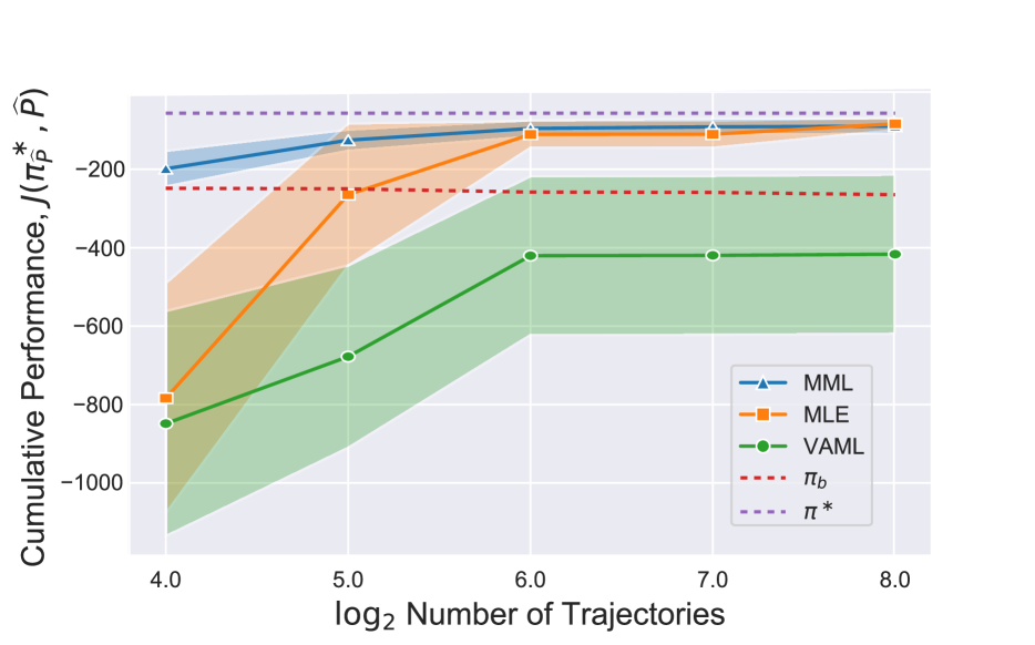
Figure 4: (Invert. Pend., OPO Performance) Comparison of model-based approaches for OPO with function-approx using Algorithm 2. Higher is better. MML performs competitively even in low data regimes.

Does our approach complement modern offline RL approaches? We integrate MML, VAML, and MLE with MOREL as in Algorithm 2. Consequently, Figure 4 shows that MML performs competitively with the other methods, achieving near-optimal performance as the number of trajectories increases. MML has good performance even in the low-data regime, whereas other methods perform worse than $\pi_{b}$. Performance in the low-data regime is of particular interest since sample efficiency is highly desirable.

Algorithm 2 forms a pessimistic MDP where a policy is penalized if it enters a state where there is disagreement between $P_{1},\ldots,P_{4}$. Given that MML performs well in low-data, we can reason that MML produces models with support that stays within the dataset $D$ or generalize well slightly outside this set. The other models poor performance is suggestive of incorrect over-confidence outside of $D$ and PPO produces a policy which takes advantage of this.

7 Other Related Work

Minimax and Model-Based RL. Rajeswaran et al. (2020) introduce an iterative minimax approach to simultaneously find the optimal-policy and a model of the environment. Despite distribution-shift correction, online data collection is required and is not comparable to MML, where we focus on the batch setting.

Batch (Offline) Model-Based RL Recent improvements in batch model-based RL focus primarily on the issue of policies taking advantage of errors in the model (Kidambi et al., 2020; Deisenroth & Rasmussen, 2011; Chua et al., 2018; Janner et al., 2019). These improvements typically involve uncertainty quantification to keep the agent in highly certain states to avoid model exploitation. These improvements are independent of the loss function involved.

8 Discussion and Future Work

We have presented a novel approach to learning a model for batch, off-policy model-based reinforcement learning. Our approach follows naturally from the definitions of the OPE and OPO objectives and enjoys distributional robustness and decision-awareness. We examined different scenarios under which our method coincided with other methods as well as when closed form solutions were available. We provided sample complexity analysis and misspecification analysis. Finally, we empirically validated that our method was competitive with current model learning approaches.

A key component throughout this paper has been the function class $\mathcal{W}\times\mathcal{V}$. Finding other interpretations for this term may prove to be useful outside of MML and is of interest in future work. Furthermore, MML remains part of a two-step OPO pipeline: first learn the model, then return the optimal policy in that model. Another direction of future research is to have a single-shot batch OPO objective that returns both a model and the optimal policy simultaneously, in effect combining MML with the minimax algorithm in Rajeswaran et al. (2020). Finally, it may be interesting to integrate MML with other forms of distributionally robust model learning, e.g., Liu et al. (2020).

Acknowledgements

Cameron Voloshin is supported in part by a Kortschak Fellowship. This work is also supported in part by NSF # 1645832, NSF # 1918839, and funding from Beyond Limits. Nan Jiang is sponsored in part by the DEVCOM Army Research Laboratory under Cooperative Agreement W911NF-17-2-0196 (ARL IoBT CRA). The views and conclusions contained in this document are those of the authors and should not be interpreted as representing the official policies, either expressed or implied, of the Army Research Laboratory or the U.S. Government. The U.S. Government is authorized to reproduce and distribute reprints for Government purposes notwithstanding any copyright notation herein.

Contents

1. 1 Introduction
2. 2 Preliminaries
3. 3 Minimax Model Learning (MML) for Off-Policy Evaluation (OPE)
   1. 3.1 Natural Derivation
   2. 3.2 Interpretation and Verifiability
   3. 3.3 Comparison to Model-Free OPE
   4. 3.4 Misspecification of $\mathcal{P},\mathcal{V},\mathcal{W}$
   5. 3.5 Application to the Online Setting
4. 4 Off-Policy Optimization (OPO)
   1. 4.1 Natural Derivation
   2. 4.2 Interpretation and Verifiability
   3. 4.3 Comparison to Model-Free OPO
5. 5 Scenarios & Considerations
   1. 5.1 Linear & Tabular Function Classes
   2. 5.2 Linear Quadratic Regulator (LQR)
   3. 5.3 Residual Dynamics & Environment Shift
   4. 5.4 Incorporating Kernels
6. 6 Experiments
   1. 6.1 Brief Environment Description/Setup
   2. 6.2 Results
7. 7 Other Related Work
8. 8 Discussion and Future Work
9. A Glossary of Terms
10. B OPE
    1. B.1 Main Result
    2. B.2 Sample Complexity for OPE

Appendix A Glossary of Terms

Table 1: Glossary of terms

Acronym	Term
OPE	Off Policy (Policy) Evaluation
OPO	Off Policy (Policy) Optimization. Also goes by batch off-policy reinforcement learning.
$\mathcal{S}$	State Space
$\mathcal{A}$	Action Space
$P$	Transition Function
$P^{\ast}$	True Transition Function
$\mathcal{R}$	Reward Function
$\mathcal{X}$	State-Action Space $\mathcal{S}\times\mathcal{A}$
$\gamma$	Discount Factor
$\pi$	Policy
$J(\pi,P)$	Performance of $\pi$ in $P$
$V^{P}_{\pi}$	Value Function of $\pi$ with respect to $P$
$d_{0}$	Initial State Distribution
$d_{\pi}^{P,\gamma}$	(Discounted) Distribution of State-Action Pairs Induced by Running $\pi$ in $P$
$w^{P}_{\pi}$	Distribution Shift ($w^{P}_{\pi}(s,a)=\frac{d_{\pi}^{P,\gamma}(s,a)}{D_{\pi_{b}}(s,a)}$)
$\nu$	Lebesgue measure
$d_{\pi_{b}}$	Behavior state distribution
$\pi_{b}$	Behavior policy
$D_{\pi_{b}}$	Behavior data ($d_{\pi_{b}}\pi_{b}$)
$D$	Dataset containing samples from $D_{\pi_{b}}P^{\ast}$
$E_{n}[\cdot]$	Empirical approximation using $D$
$E[\cdot]$	Exact expectation
$\mathcal{W}$	Distribution Shifts Function Class (e.g. $\frac{d_{\pi}^{P}(s,a)}{D_{\pi}(s,a)}$)
$\mathcal{V}$	Value Function Class (e.g. $V^{P}_{\pi}\in\mathcal{V})$
$\mathcal{P}$	Model Function Class (e.g. $P\in\mathcal{P})$
$\mathcal{L}$	Model Learning Loss Function
$\widehat{P}$	Best Model w.r.t $\mathcal{L}$
$\epsilon_{\mathcal{H}}$	Misspecification Error
$\pi^{\ast}_{P}$	Optimal Policy in $P$
RKHS	Reproducing Kernel Hilbert Space
LQR	Linear Quadratic Regulator
IP	Inverted Pendulum
MML	Minimax Model Learning (Ours)
MLE	Maximum Likelihood Estimation
VAML	Value-Aware Model Learning

Appendix B OPE

In this section we explore the OPE results in the order in which they were presented in the main paper.

B.1 Main Result

Proof for Theorem 3.1.

Assume $(w^{P^{\ast}}_{\pi},V^{P}_{\pi})\in\mathcal{W}\times\mathcal{V}$. Fix some $P\in\mathcal{P}$. We use both definitions of $J$ as follows

$$J(\pi,P)-J(\pi,P^{\ast}) =E_{d_{0}}[V^{P}_{\pi}]-E_{(s,a)\sim d^{P^{\ast}}_{\pi,\gamma},r\sim\mathcal{R}(\cdot|s,a)}[r]$$

$$=E_{(s,a)\sim d^{P^{\ast}}_{\pi,\gamma}}[V^{P}_{\pi}(s)-E_{r\sim\mathcal{R}(\cdot|s,a)}[r]]+E_{d_{0}}[V^{P}_{\pi}]-E_{(s,a)\sim d^{P^{\ast}}_{\pi,\gamma}}[V^{P}_{\pi}(s)]$$

$$=E_{(s,a)\sim d^{P^{\ast}}_{\pi,\gamma}}[V^{P}_{\pi}(s)-E_{r\sim\mathcal{R}(\cdot|s,a)}[r]]-\sum_{t=1}^{\infty}\gamma^{t}\int d^{P^{\ast}}_{\pi,t}(s,a)V^{P}_{\pi}(s)d\nu(s,a)$$

$$=E_{(s,a)\sim d^{P^{\ast}}_{\pi,\gamma}}[\gamma E_{s^{\prime}\sim P(\cdot|s,a)}[V^{P}_{\pi}(s^{\prime})]]-\gamma\sum_{t=0}^{\infty}\gamma^{t}\int d^{P^{\ast}}_{\pi,t+1}(s,a)V^{P}_{\pi}(s)d\nu(s,a)$$

$$=\gamma E_{(s,a)\sim d^{P^{\ast}}_{\pi,\gamma}}[E_{s^{\prime}\sim P(\cdot|s,a)}[V^{P}_{\pi}(s^{\prime})]]-\gamma\sum_{t=0}^{\infty}\gamma^{t}\int d^{P^{\ast}}_{\pi,t}(\tilde{s},\tilde{a})P^{\ast}(s|\tilde{s},\tilde{a})\pi(a|s)V^{P}_{\pi}(s)d\nu(\tilde{s},\tilde{a},s,a)$$

$$=\gamma E_{(s,a)\sim d^{P^{\ast}}_{\pi,\gamma}}[E_{s^{\prime}\sim P(\cdot|s,a)}[V^{P}_{\pi}(s^{\prime})]]-\gamma\sum_{t=0}^{\infty}\gamma^{t}\int d^{P^{\ast}}_{\pi,t}(s,a)P^{\ast}(s^{\prime}|s,a)V^{P}_{\pi}(s^{\prime})d\nu(s,a,s^{\prime})$$

$$=\gamma E_{(s,a)\sim d^{P^{\ast}}_{\pi,\gamma}}[E_{s^{\prime}\sim P(\cdot|s,a)}[V^{P}_{\pi}(s^{\prime})]]-\gamma E_{(s,a)\sim d^{P^{\ast}}_{\pi,\gamma}}[E_{s^{\prime}\sim P^{\ast}(\cdot|s,a)}[V^{P}_{\pi}(s^{\prime})]]$$

$$=\gamma E_{(s,a)\sim d^{P^{\ast}}_{\pi,\gamma}}[E_{s^{\prime}\sim P(\cdot|s,a)}[V^{P}_{\pi}(s^{\prime})]-E_{s^{\prime}\sim P^{\ast}(\cdot|s,a)}[V^{P}_{\pi}(s^{\prime})]]$$

$$=\gamma E_{(s,a,s^{\prime})\sim D_{\pi_{b}}P^{\ast}(\cdot|s,a)}[\frac{d^{P^{\ast}}_{\pi,\gamma}(s,a)}{D_{\pi_{b}}(s,a)}\left(E_{x\sim P(\cdot|s,a)}[V^{P}_{\pi}(x)]-V^{P}_{\pi}(s^{\prime})\right)]]$$

$$=\gamma E_{(s,a,s^{\prime})\sim D_{\pi_{b}}P^{\ast}(\cdot|s,a)}[w^{P^{\ast}}_{\pi}(s,a)\left(E_{x\sim P(\cdot|s,a)}[V^{P}_{\pi}(x)]-V^{P}_{\pi}(s^{\prime})\right)]]$$

$$=\gamma\mathcal{L}(w^{P^{\ast}}_{\pi},V^{P}_{\pi},P),$$

where the first equality is definition. The second equality is addition of $0$. The third equality is simplification. The fourth equality is change of bounds. The fifth is definition. The sixth is relabeling of the integration variables. The seventh and eighth are simplification. The ninth is importance sampling. The tenth and last is definition. Since $(w^{P^{\ast}}_{\pi},V^{P}_{\pi})\in\mathcal{W}\times\mathcal{V}$ then

$$|J(\pi,P)-J(\pi,P^{\ast})|=\gamma|\mathcal{L}(w^{P^{\ast}}_{\pi},V^{P}_{\pi},P)|\leq\gamma\max_{w\in\mathcal{W},V\in\mathcal{V}}|\mathcal{L}(w,V,P)|\leq\gamma\min_{P\in\mathcal{P}}\max_{w\in\mathcal{W},V\in\mathcal{V}}|\mathcal{L}(w,V,P)|,$$

where the last inequality holds because $P$ was selected in $\mathcal{P}$ arbitrarily.

Now, instead, assume $(w^{P}_{\pi},V^{P^{\ast}}_{\pi})\in\mathcal{W}\times\mathcal{V}$. Fix some $P\in\mathcal{P}$. Then, similarly,

$$J(\pi,P)-J(\pi,P^{\ast}) =E_{(s,a)\sim d^{P}_{\pi,\gamma},r\sim\mathcal{R}(\cdot|s,a)}[r]-E_{d_{0}}[V^{P^{\ast}}_{\pi}]$$

$$=E_{(s,a)\sim d^{P}_{\pi,\gamma}}[V^{P^{\ast}}_{\pi}(s)]-E_{d_{0}}[V^{P^{\ast}}_{\pi}]-E_{(s,a)\sim d^{P}_{\pi,\gamma}}[V^{P^{\ast}}_{\pi}(s)-E_{r\sim\mathcal{R}(\cdot|s,a)}[r]]$$

$$=\sum_{t=1}^{\infty}\gamma^{t}\int d^{P}_{\pi,t}(s,a)V^{P^{\ast}}_{\pi}(s)d\nu(s,a)-E_{(s,a)\sim d^{P}_{\pi,\gamma}}[V^{P^{\ast}}_{\pi}(s)-E_{r\sim\mathcal{R}(\cdot|s,a)}[r]]$$

$$=\gamma\sum_{t=0}^{\infty}\gamma^{t}\int d^{P}_{\pi,t+1}(s,a)V^{P^{\ast}}_{\pi}(s)d\nu(s,a)-E_{(s,a)\sim d^{P}_{\pi,\gamma}}[\gamma E_{s^{\prime}\sim P^{\ast}(\cdot|s,a)}[V^{P^{\ast}}_{\pi}(s^{\prime})]]$$

$$=\gamma\sum_{t=0}^{\infty}\gamma^{t}\int d^{P}_{\pi,t}(\tilde{s},\tilde{a})P(s|\tilde{s},\tilde{a})\pi(a|s)V^{P^{\ast}}_{\pi}(s)d\nu(\tilde{s},\tilde{a},s,a)-\gamma E_{(s,a)\sim d^{P}_{\pi,\gamma}}[E_{s^{\prime}\sim P^{\ast}(\cdot|s,a)}[V^{P^{\ast}}_{\pi}(s^{\prime})]]$$

$$=\gamma\sum_{t=0}^{\infty}\gamma^{t}\int d^{P}_{\pi,t}(s,a)P(s^{\prime}|s,a)V^{P^{\ast}}_{\pi}(s^{\prime})d\nu(s,a,s^{\prime})-\gamma E_{(s,a)\sim d^{P}_{\pi,\gamma}}[E_{s^{\prime}\sim P^{\ast}(\cdot|s,a)}[V^{P^{\ast}}_{\pi}(s^{\prime})]]$$

$$=\gamma E_{(s,a)\sim d^{P}_{\pi,\gamma}}[E_{s^{\prime}\sim P(\cdot|s,a)}[V^{P^{\ast}}_{\pi}(s^{\prime})]]-\gamma E_{(s,a)\sim d^{P}_{\pi,\gamma}}[E_{s^{\prime}\sim P^{\ast}(\cdot|s,a)}[V^{P^{\ast}}_{\pi}(s^{\prime})]]$$

$$=\gamma E_{(s,a)\sim d^{P}_{\pi,\gamma}}[E_{s^{\prime}\sim P(\cdot|s,a)}[V^{P^{\ast}}_{\pi}(s^{\prime})]-E_{s^{\prime}\sim P^{\ast}(\cdot|s,a)}[V^{P^{\ast}}_{\pi}(s^{\prime})]]$$

$$=\gamma E_{(s,a,s^{\prime})\sim D_{\pi_{b}}P^{\ast}(\cdot|s,a)}[\frac{d^{P}_{\pi,\gamma}(s,a)}{D_{\pi_{b}}(s,a)}\left(E_{x\sim P(\cdot|s,a)}[V^{P^{\ast}}_{\pi}(x)]-V^{P^{\ast}}_{\pi}(s^{\prime})\right)]]$$

$$=\gamma E_{(s,a,s^{\prime})\sim D_{\pi_{b}}P^{\ast}(\cdot|s,a)}[w^{P}_{\pi}(s,a)\left(E_{x\sim P(\cdot|s,a)}[V^{P^{\ast}}_{\pi}(x)]-V^{P^{\ast}}_{\pi}(s^{\prime})\right)]]$$

$$=\gamma\mathcal{L}(w^{P}_{\pi},V^{P^{\ast}}_{\pi},P),$$

where we follow the same steps as in the previous derivation. Since $(w^{P}_{\pi},V^{P^{\ast}}_{\pi})\in\mathcal{W}\times\mathcal{V}$ then

$$|J(\pi,P)-J(\pi,P^{\ast})|=\gamma|\mathcal{L}(w^{P}_{\pi},V^{P^{\ast}}_{\pi},P)|\leq\gamma\max_{w\in\mathcal{W},V\in\mathcal{V}}|\mathcal{L}(w,V,P)|\leq\gamma\min_{P\in\mathcal{P}}\max_{w\in\mathcal{W},V\in\mathcal{V}}|\mathcal{L}(w,V,P)|,$$

where the last inequality holds because $P$ was selected in $\mathcal{P}$ arbitrarily. ∎

B.2 Sample Complexity for OPE

We do not have access to exact expectations, so we must work with $\widehat{P}_{n}=\arg\min_{P}\max_{w,V}E_{n}[\ldots]$ instead of $\widehat{P}=\arg\min_{P}\max_{w,V}E[\ldots]$. Furthermore, $J(\pi,\widehat{P})$ requires exact expectation of an infinite sum: $E_{d_{0}}[\sum_{t=0}^{\infty}\gamma^{t}r_{t}]$ where we collect $r_{t}$ by running $\pi$ in simulation $\widehat{P}$. Instead, we can only estimate an empirical average over a finite sum in $\widehat{P}_{n}$: $J_{T,m}(\pi,\widehat{P}_{n})=\frac{1}{m}\sum_{j=1}^{m}\sum_{t=0}^{T}\gamma^{t}r^{j}_{t}$, where each $j$ indexes rollouts starting from $s_{0}\sim d_{0}$ and the simulation is over $\widehat{P}_{n}$. Our OPE estimate is therefore bounded as follows:

Theorem B.1.

[OPE Error] Let the functions in $\mathcal{V}$ and $\mathcal{W}$ be uniformly bounded by $C_{\mathcal{V}}$ and $C_{\mathcal{W}}$ respectively. Assume the conditions of Theorem 3.1 hold and $|\mathcal{R}|\leq R_{\text{max}},\gamma\in[0,1)$. Then, with probability $1-\delta$,

$$| J_{T,m}(\pi,\widehat{P}_{n})-J(\pi,P^{\ast})|\leq\gamma\min_{P}\max_{w,V}|\mathcal{L}(w,V,P)|$$

$$+4\gamma\mathfrak{R}_{n}(\mathcal{W},\mathcal{V},\mathcal{P})+\frac{2R_{\text{max}}}{1-\gamma}\gamma^{T+1}$$

$$+\frac{2R_{\text{max}}}{1-\gamma}\sqrt{\log(2/\delta)/(2m)}+4\gamma C_{\mathcal{W}}C_{\mathcal{V}}\sqrt{\log(2/\delta)/n}$$

where $\mathfrak{R}_{n}(\mathcal{W},\mathcal{V},\mathcal{P})$ is the Rademacher complexity of the function class

$$\{(s,a,s^{\prime})\mapsto w(s,a)(E_{x\sim P}[V(x)]-V(s^{\prime})):$$

$$w\in\mathcal{W},V\in\mathcal{V},P\in\mathcal{\mathcal{P}}\}.$$

Proof for Theorem B.1.

By definition and triangle inequality, Δ—J_T,m(π,^P_n ) - J(π,P^∗)— &= — J_T,m(π,^P_n ) - J(π,^P_n) + J(π,^P_n) - J(π,P^∗)—  
≤⏟— J_T,m(π,^P_n ) - J(π,^P_n )—_(a) + ⏟—J(π,^P_n ) - J(π,P^∗)—_(b)

Define $\widehat{V}_{\pi,T}^{P}(s_{0}^{i})\equiv\sum_{t=0}^{T}\gamma^{t}r_{t}^{i}$ for some trajectory indexed by $i\in\mathbb{N}$ where $r_{t}^{i}$ is the reward obtained by running $\pi$ in $P$ at time $t\leq T$ starting at $s_{0}^{i}$. For $(a)$, Δ— J_T,m(π,^P_n ) - J(π,^P_n )— &= — 1m ∑_i=1^m ^V^^P_n _π, T (s_0^i) - 1m ∑_i=1^m ^V^^P_n _π, ∞ (s_0^i) + 1m ∑_i=1^m ^V^^P_n _π, ∞ (s_0^i) - E_d_0[V^^P_n _π] —
≤— 1m ∑_i=1^m ^V^^P_n _π, T (s_0^i) - 1m ∑_i=1^m ^V^^P_n _π, ∞ (s_0^i)— + —1m ∑_i=1^m ^V^^P_n _π, ∞ (s_0^i) - E_d_0[V^^P_n _π] —
≤2 Rmax1-γ γ^T+1 + 2 Rmax1-γlog(2/δ)/(2m), with probability $1-\delta$, where the last inequality is definition of $\widehat{V}_{\pi,T}$ and Hoeffding’s inequality.

For $(b)$, by Theorem 3.1, Δ—J&(π,^P_n ) - J(π,P^∗)—
= γ—L(w_π^P^∗, V^^P_n, ^P_n)—
≤γmax_w,V —L(w, V, ^P_n)—
= γ(max_w,V —L(w, V, ^P_n)— - max_w,V —L_n(w, V, ^P_n)— + max_w,V —L_n(w, V, ^P_n)— - max_w,V —L(w, V, ^P)— + max_w,V —L(w, V, ^P)—)
≤γ( 2 max

References

- Abachi et al. (2020) Abachi, R., Ghavamzadeh, M., and massoud Farahmand, A. Policy-aware model learning for policy gradient methods, 2020.
- Antos et al. (2008) Antos, A., Szepesvári, C., and Munos, R. Learning near-optimal policies with bellman-residual minimization based fitted policy iteration and a single sample path. Machine Learning, 71(1):89–129, 2008.
- Bartlett & Mendelson (2001) Bartlett, P. L. and Mendelson, S. Rademacher and gaussian complexities: Risk bounds and structural results. In Proceedings of the 14th Annual Conference on Computational Learning Theory and and 5th European Conference on Computational Learning Theory, Berlin, Heidelberg, 2001. Springer-Verlag. ISBN 3540423435.
- Bertsekas et al. (2005) Bertsekas, D. P., Bertsekas, D. P., Bertsekas, D. P., and Bertsekas, D. P. Dynamic programming and optimal control, volume 1. Athena scientific Belmont, MA, 2005.
- Brockman et al. (2016) Brockman, G., Cheung, V., Pettersson, L., Schneider, J., Schulman, J., Tang, J., and Zaremba, W. Openai gym. CoRR, abs/1606.01540, 2016.
- Chen & Jiang (2019) Chen, J. and Jiang, N. Information-theoretic considerations in batch reinforcement learning. In Chaudhuri, K. and Salakhutdinov, R. (eds.), Proceedings of the 36th International Conference on Machine Learning, Long Beach, California, USA, 09–15 Jun 2019. PMLR.
- Chua et al. (2018) Chua, K., Calandra, R., McAllister, R., and Levine, S. Deep reinforcement learning in a handful of trials using probabilistic dynamics models. In Bengio, S., Wallach, H., Larochelle, H., Grauman, K., Cesa-Bianchi, N., and Garnett, R. (eds.), Advances in Neural Information Processing Systems 31. Curran Associates, Inc., 2018.
- Clavera et al. (2018) Clavera, I., Rothfuss, J., Schulman, J., Fujita, Y., Asfour, T., and Abbeel, P. Model-based reinforcement learning via meta-policy optimization. In 2nd Annual Conference on Robot Learning, CoRL 2018, Zürich, Switzerland, 29-31 October 2018, Proceedings. PMLR, 2018.
- Deisenroth & Rasmussen (2011) Deisenroth, M. P. and Rasmussen, C. E. Pilco: A model-based and data-efficient approach to policy search. In Proceedings of the 28th International Conference on International Conference on Machine Learning, Madison, WI, USA, 2011. Omnipress. ISBN 9781450306195.
- Dorobantu & Taylor (2020) Dorobantu, V. and Taylor, A. Lyapy. https://github.com/vdorobantu/lyapy, 2020.
- Ernst et al. (2005) Ernst, D., Geurts, P., and Wehenkel, L. Tree-based batch mode reinforcement learning. J. Mach. Learn. Res., 6:503–556, December 2005. ISSN 1532-4435.
- Farahmand (2018) Farahmand, A.-m. Iterative value-aware model learning. In Bengio, S., Wallach, H., Larochelle, H., Grauman, K., Cesa-Bianchi, N., and Garnett, R. (eds.), Advances in Neural Information Processing Systems 31, 9072–9083. Curran Associates, Inc., 2018.
- Farahmand et al. (2017) Farahmand, A.-M., Barreto, A., and Nikovski, D. Value-Aware Loss Function for Model-based Reinforcement Learning. In Singh, A. and Zhu, J. (eds.), Proceedings of the 20th International Conference on Artificial Intelligence and Statistics, Fort Lauderdale, FL, USA, 20–22 Apr 2017. PMLR.
- Feng et al. (2019) Feng, Y., Li, L., and Liu, Q. A kernel loss for solving the bellman equation. In Advances in Neural Information Processing Systems, 2019.
- (15) Goodfellow, I., Bengio, Y., and Courville, A. Deep Learning. MIT Press.
- Goodfellow et al. (2014) Goodfellow, I., Pouget-Abadie, J., Mirza, M., Xu, B., Warde-Farley, D., Ozair, S., Courville, A., and Bengio, Y. Generative adversarial nets. In Ghahramani, Z., Welling, M., Cortes, C., Lawrence, N. D., and Weinberger, K. Q. (eds.), Advances in Neural Information Processing Systems 27, 2672–2680. Curran Associates, Inc., 2014.
- Janner et al. (2019) Janner, M., Fu, J., Zhang, M., and Levine, S. When to trust your model: Model-based policy optimization. In Wallach, H., Larochelle, H., Beygelzimer, A., d'Alché-Buc, F., Fox, E., and Garnett, R. (eds.), Advances in Neural Information Processing Systems 32, 12519–12530. Curran Associates, Inc., 2019.
- Kidambi et al. (2020) Kidambi, R., Rajeswaran, A., Netrapalli, P., and Joachims, T. Morel : Model-based offline reinforcement learning, 2020.
- Kingma & Ba (2015) Kingma, D. P. and Ba, J. Adam: A method for stochastic optimization. In Bengio, Y. and LeCun, Y. (eds.), 3rd International Conference on Learning Representations, ICLR 2015, San Diego, CA, USA, May 7-9, 2015, Conference Track Proceedings, 2015.
- Kurutach et al. (2018) Kurutach, T., Clavera, I., Duan, Y., Tamar, A., and Abbeel, P. Model-ensemble trust-region policy optimization. In 6th International Conference on Learning Representations, ICLR 2018, Vancouver, BC, Canada, April 30 - May 3, 2018, Conference Track Proceedings. OpenReview.net, 2018.
- Liu et al. (2020) Liu, A., Shi, G., Chung, S.-J., Anandkumar, A., and Yue, Y. Robust regression for safe exploration in control. In Learning for Dynamics and Control (L4DC), 2020.
- Liu et al. (2018) Liu, Q., Li, L., Tang, Z., and Zhou, D. Breaking the curse of horizon: Infinite-horizon off-policy estimation. In Advances in Neural Information Processing Systems, 2018.
- Luo et al. (2019) Luo, Y., Xu, H., Li, Y., Tian, Y., Darrell, T., and Ma, T. Algorithmic framework for model-based deep reinforcement learning with theoretical guarantees. In 7th International Conference on Learning Representations, ICLR 2019, New Orleans, LA, USA, May 6-9, 2019. OpenReview.net, 2019.
- MacKay (2002) MacKay, D. J. C. Information Theory, Inference & Learning Algorithms. Cambridge University Press, USA, 2002. ISBN 0521642981.
- Mohri et al. (2012) Mohri, M., Rostamizadeh, A., and Talwalkar, A. Foundations of machine learning. MIT press, 2012.
- Raffin et al. (2019) Raffin, A., Hill, A., Ernestus, M., Gleave, A., Kanervisto, A., and Dormann, N. Stable baselines3. https://github.com/DLR-RM/stable-baselines3, 2019.
- Rajeswaran et al. (2020) Rajeswaran, A., Mordatch, I., and Kumar, V. A game theoretic framework for model based reinforcement learning, 2020.
- Schaefer & Anandkumar (2019) Schaefer, F. and Anandkumar, A. Competitive gradient descent. In Wallach, H., Larochelle, H., Beygelzimer, A., d'Alché-Buc, F., Fox, E., and Garnett, R. (eds.), Advances in Neural Information Processing Systems 32, 7625–7635. Curran Associates, Inc., 2019.
- Schulman et al. (2017) Schulman, J., Wolski, F., Dhariwal, P., Radford, A., and Klimov, O. Proximal policy optimization algorithms. CoRR, abs/1707.06347, 2017.
- Sutton (1990) Sutton, R. S. Integrated architectures for learning, planning, and reacting based on approximating dynamic programming. In In Proceedings of the Seventh International Conference on Machine Learning. Morgan Kaufmann, 1990.
- Uehara et al. (2020) Uehara, M., Huang, J., and Jiang, N. Minimax Weight and Q-Function Learning for Off-Policy Evaluation. In Proceedings of the 37th International Conference on Machine Learning, 2020.
- Voloshin et al. (2019) Voloshin, C., Le, H. M., Jiang, N., and Yue, Y. Empirical study of off-policy policy evaluation for reinforcement learning. arXiv preprint arXiv:1911.06854, 2019.