A continuous-state cellular automata algorithm for global optimization

Abstract

Cellular automata are capable of developing complex behaviors based on simple local interactions between their elements. Some of these characteristics have been used to propose and improve meta-heuristics for global optimization; however, the properties offered by the evolution rules in cellular automata have not yet been used directly in optimization tasks. Inspired by the complexity that various evolution rules of cellular automata can offer, the continuous-state cellular automata algorithm (CCAA) is proposed. In this way, the CCAA takes advantage of different evolution rules to maintain a balance that maximizes the exploration and exploitation properties in each iteration. The efficiency of the CCAA is proven with $33$ test problems widely used in the literature, $4$ engineering applications that were also used in recent literature, and the design of adaptive infinite-impulse response (IIR) filters, testing $10$ full-order IIR reference functions. The numerical results prove its competitiveness in comparison with state-of-the-art algorithms. The source codes of the CCAA are publicly available at https://github.com/juanseck/CCAA.git.

Keywords: global optimization, cellular automata, meta-heuristics, engineering applications

Submitted to Expert Systems With Applications

1 Introduction

Nowadays, the constant demand for reducing costs and production times and the unstoppable competition in the engineering area has driven the search for advanced decision-making methods, such as optimization methods, to design and produce goods economically and efficiently. Among these optimization methods are meta-heuristics, which are high-level algorithms with which good enough solutions to optimization problems can be found. (Kumar and Davim, 2020).

Meta-heuristic algorithms are of great relevance because, in general, they are easy to implement and their operation is based on simple concepts that do not require information regarding the gradient of the function to be optimized. A good meta-heuristic algorithm can escape from local optima and be used in a wide range of optimization, design, and parameter identification problems.

For that purpose, meta-heuristic algorithms must perform in an efficient and balanced way the exploration of the solution space and the exploitation of promising areas of said space. Since these actions can conflict and leave the algorithm trapped in a local minimum, the correct balance of both processes is essential to obtain a meta-heuristic algorithm that calculates good solutions, avoiding stagnation or premature convergence towards local minima.

The optimization problem, which consists of finding the best sets of parameters that optimize a given objective function, subject to restrictions, has been approached from different perspectives. One of them is represented by algorithms inspired by physical and natural systems, with variants and modifications that intensify their exploitation and exploration characteristics. One of the best-known algorithms is the genetic algorithm (GA) (Holland, 1984), which has been hybridized and adapted multiple times to optimize a broader range of problems. An example is where it is combined with neural networks to enhance the capacity to optimize complex nonlinear problems (Qiao et al., 2020). Another example is the particle swarm optimization (PSO) algorithm (Eberhart and Kennedy, 1995), in which, unlike the GA, all particles have memory and share knowledge. Like the GA, it has been modified and improved multiple times; for example, in the study by (Yang et al., 2020), PSO was improved based on entropy, which reduces the swarm’s randomness and increases the diversity of the population. An algorithm that can be considered a modification and hybridization of the GA and the PSO (Yang et al., 2020) is the differential evolution (DE) algorithm, which treats individuals as strings of real numbers, making encoding and decoding for continuous problems unnecessary. In the case of the DE, we can also find multiple modifications and improvements, such as proposing a dual strategy strengthening global exploration and population diversity (Zhong and Cheng, 2020).

Another algorithm based on non-trivial collective behavior that originates from sharing information among the population members is the ant colony optimization algorithm (ACO) (Dorigo and Gambardella, 1997). ACO has been studied deeply and multiple recent variants have been presented (Chatterjee et al., 2020) (Liu et al., 2020) (Yu et al., 2020). Another algorithm inspired by the global behavior that performs a complex task, such as foraging, based on its individuals’ interactions, is the artificial bee colony algorithm (ABC) (Karaboga, 2005). In the same way, many variants and improvements have been recently proposed (Huang et al., 2019) (Wang et al., 2020), which shows that algorithms based on population behaviors continue to be an active research area.

In addition to the variants and modifications of population-based algorithms, we can find in the recent literature various works where algorithms are hybridized to enhance the search properties for particular cases (Lagos-Eulogio et al., 2017) (Qiao et al., 2020) (Qu et al., 2020) (Moayedi et al., 2020) or those that adapt not only the parameters but also the procedure used, such as the drone squad optimization (DSO) algorithm (de Melo and Banzhaf, 2018).

Meta-heuristic algorithms have shown great capacity and adaptability in finding global minima in different test problems and practical applications over the years. However, these types of algorithms are always in constant improvement since according to the No Free Lunch (NFL) theorem, no meta-heuristic can optimize all kinds of problems (Wolpert and Macready, 1997). As a result of the need to optimize increasingly complex problems with a larger number of dimensions, the emergence of new meta-heuristic algorithms has increased in recent years (Tansel Dokeroglua and Cosarb, 2019).

In this work, a new meta-heuristic algorithm based on the neighborhood concept and evolution rules of cellular automata is proposed for the global optimization of problems defined in multiple dimensions. As this algorithm uses continuous variables, it has been named the continuous cellular automata algorithm (CCAA).

The algorithm defines a set of initial solutions, each one of which generates a neighborhood of possible new solutions to improve the fitness (or cost) of these solutions concerning the problem to be optimized, which, in the case of this work, is the minimization of functions. This neighborhood is formed using rules inspired by cellular automata, where some of them serve to exchange information with other solutions and others only take information from the solution and the best cost obtained to induce changes in its elements.

The contribution of the CCAA lies in the direct use of the concepts of neighborhood and evolution rule in the dynamics of the solutions to carry out the optimization process. These features lead to the implementation of an algorithm that is very simple to implement and which, at the same time, is highly competitive compared to other recently published algorithms with proven performance.

There are many meta-heuristics applications in the area of engineering since they have been used with satisfactory results in complex tasks such as the identification of system parameters from experimental data, the optimal modeling of materials, and multi-dimensional optimization, to mention a few (Kumar and Davim, 2020). Examples of these applications are mechanical gear train design, helical compression spring design (Sandgren, 1990), pressure vessel design (Sandgren, 1990) (Salih et al., 2019), process control (Mukhtar et al., 2019), and the design of adaptive digital filters, one of the more popular application fields in recent years due to its relevance to real-world problems (Jiang et al., 2015) (Lagos-Eulogio et al., 2017) (Atul Kumar Dwivedi and Londhe, 2018). The operation of the CCAA is tested using some of these applications to check its performance against other specialized algorithms.

The structure of the paper is as follows. Section 2 describes the basic concepts of cellular automata, the proposals for meta-heuristic algorithms based on cellular automata, and the opportunity to improve this type of implementations. Section 3 presents the CCAA algorithm and explains the adaptations of various evolution rules to carry out exploration and exploitation tasks concurrently as well as the general strategy of the CCAA. Section 4 shows the experimental results of $33$ test functions in $30$ and $500$ dimensions, presenting a statistical comparison with other state-of-the-art algorithms. Section 4.4 applies the CCAA in $4$ engineering problems that are commonly considered in the specialized literature, in addition to utilizing the proposed algorithm in the design of adaptive IIR filters of full order. These results are compared with previously published findings to show the effectiveness and performance of the CCAA. The last section provides the conclusions and future proposals for the development of the CCAA.

2 Preliminaries

A cellular automaton is a discrete dynamical system composed of cells that initially take their values from a finite set of possible states. The dynamics of the system is given in discrete steps. In each step, a cell takes into account its current state and those of its neighbors to update its state. This assignment of neighborhoods to states is known as the evolution rule. Thus, a cellular automaton is discrete in time and space.

Cellular automata are easy to implement in a computer, given the simplicity of their specification. However, these systems can develop chaotic and complex global behaviors, which have been widely investigated and used to solve various computational and engineering problems (McIntosh, 2009) (Wolfram, 2002). Fig. 1 shows the evolutions of different cellular automata with $4$ states, with distinct dynamical behaviors.

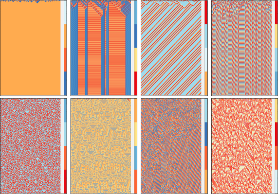
Figure 1: Examples of different cellular automata with $4$ states

Although concepts and ideas of cellular automata have been used before for proposing new meta-heuristics, very few have used the main concept that characterizes a cellular automaton, the simplicity of its neighborhood, and the versatility that can be found in its evolution rules. One of the most recent works that uses the concept of neighborhood in cellular automata to propose a global optimization meta-heuristic is the cellular particle swarm optimization (CPSO) (Shi et al., 2011). CPSO has been shown to be very useful for global optimization tasks, although the proposed evolution rule continues to be based on an adaptation of the classical PSO equations. Other recent meta-heuristics were proposed for the implementation of cellular automata concepts oriented to particular engineering problems, such as for the design of adaptive IIR filters (Lagos-Eulogio et al., 2017) and for the simultaneous optimization of the plant layout and the sequencing of tasks in a job-shop-type system (Hernández-Gress et al., 2020).

However, the versatility of the evolution rules that are widely used in cellular automata for various modeling problems and for computational complexity has not been directly adapted in an algorithm for global optimization tasks. This is the main contribution of this paper, whose implementation is described in the next section.

3 Continuous cellular automata algorithm (CCAA)

The evolution rules of cellular automata have been widely studied for the complex behaviors they represent, model, and construct. Within these rules, we can find that globally, cellular automata can generate periodic, chaotic, complex, reversible behaviors or are capable of solving complex global tasks such as global synchronization, classification, or task scheduling problems.

The aim is to take these types of rules as inspiration to adapt them into an optimization algorithm, where solutions are able to share information and generate spontaneous changes that are useful in carrying out exploration and exploitation tasks in a solution space.

The function that is to be optimized (in this work, the case of minimization is taken) is defined as $f(\mathbf{x})\rightarrow\mathbb{R}$ in $n$ dimensions, where $x\in\mathbb{R}^{n}$ and each $x_{i}$ value in $\mathbf{x}$ is bounded between a lower bound $lb_{i}$ and an upper bond $ub_{i}$. If the bounds are the same for all the values of $\mathbf{x}$, then these limit values will simply be stated as $lb$ and $ub$.

The CCAA first takes an initial population $S$ of $smart\_n$ initial solutions or $smart\_cells$. Each $smart\_cell$ is represented as $s\in\mathbb{R}^{n}$ and its cost is given by $f(\mathbf{s})$. Given a population $S$, the best solution will be represented as $b_{S}$ such that its cost $f(b_{S})$ is minimal with respect to all the other $smart\_cells$ in $S$.

The algorithm uses a total of $12$ evolution rules adapted from cellular automata to apply them on the $smart\_cells$ in $S$ and their costs in $f$. The general strategy is to generate a neighborhood of each $smart\_cell$ with $m$ neighbors and from that neighborhood, take the best solution as the new $smart\_cell$ in a probabilistic way or if it improves the cost of the original $smart\_cell$. The evolution rules used to carry out the CCAA’s exploration and exploitation actions are described in the upcoming section.

3.1 Rules for approaching a neighbor

In this type of rule, a $smart\_cell$ $s_{i}$ will approach another $smart\_cell$ $s_{j}$ depending on the cost $f(s_{i})$ and $f(s_{j})$. The structure of the rule is as follows:

Result: New $smart\_cell$ $evol$

Input: $s_{i}$, $s_{j}$, $f(s_{i})$, $f(s_{j})$, $prop$ ;

$evol=s_{i}$;

if $condition(f(s_{i}),f(s_{j}))$ then

       $dec=(s_{i}-s_{j})*prop*rand$;

      

end if

$evol=evol-dec$;

Algorithm 1 Approach rule

The rule in the Algorithm 1 is very simple: if $condition(f(s_{i}),f(s_{j}))$ is true, a vector is calculated with the difference between each element of $s_{i}$ and $s_{j}$ and the rule weights these differences by a proportion that goes between $0$ and $prop$ in a uniform random way. If the condition is false, $s_{i}$ remains unchanged.

This makes $s_{i}$ get closer to $s_{j}$ as $prop$ indicates, if this value is low the approach will be limited. This rule serves the purposes of differentiated exploitation of the elements in $s_{i}$, since the vector of differences is calculated element by element. In the CCAA, one version of this rule,$R_{1}$, is used, which takes $f(s_{i})\neq f(s_{j})$ as condition, and $prop=lower_{p}$, where $lower_{p}$ has a low value. This allows the original $s_{i}$ to be moved in its close neighborhood in the direction of a neighbor with a different cost.

3.2 Rules for staying away from a neighbor

Result: New $smart\_cell$ $evol$

Input: $s_{i}$, $s_{j}$, $f(s_{i})$, $f(s_{j})$, $prop$ ;

$evol=s_{i}$;

if $condition(f(s_{i}),f(s_{j}))$ then

       $inc=(s_{i}-s_{j})*prop*rand$;

      

end if

$evol=evol+inc$;

Algorithm 2 Rule of taking away

The rule in Algorithm 2 is also simple. If $condition(f(s_{i}),f(s_{j}))$ is true, the vector of differences $s_{i}-s_{j}$ is calculated and weighted with a uniform random value between $0$ and $prop$. If the condition is false, $s_{i}$ does not change.

This rule has the effect of moving $s_{i}$ away from $s_{j}$, which implies that if $s_{i}$ is close to $s_{j}$, then the rule can continue to exploit areas further away from the vicinity of $s_{i}$ and help to escape local minima. In the other case, where $s_{i}$ is far from $s_{j}$, then the new solution will be far from $s_{j}$ and will serve the exploration of new areas in the search space for both $s_{i}$ and $s_{j}$.

In the CCAA, two versions of this rule are used: $R_{2}$ with the condition $f(s_{i})\neq f(s_{j})$ and $prop=upper_{b}$ is considered, where $upper_{b}$ has a high value that allows for a significant difference from $s_{j}$, and $R_{3}$, which takes as condition $f(s_{i})<f(s_{j})$ and $prop=lower_{b}$, causing $s_{i}$ to deviate a little from $s_{j}$ only when the cost $f(s_{j})$ is higher. This rule serves to intensify the task of exploiting the information in $s_{i}$ in a direction away from $s_{j}$.

3.3 Rules for changes in a $smart\_cell$

Result: New $smart\_cell$ $evol$

Input: $s_{i}$, $s_{j}$, $f(s_{i})$, $f(s_{j})$, $dist$ ;

$evol=s_{i}$;

$sum=f(s_{i})+f(s_{j})$;

$pond=1-(f(s_{j})/sum)$;

$r=(rand*dist)-(dist/2)$;

forall $k$ in $length(evol)$ do

       if $rand<=pond$ then

             $evol_{k}=evol_{k}+r*s_{jk}$;

            

       end if

      

end forall

Algorithm 3 Change rule

The rule in Algorithm 3 is to estimate how optimal $s_{i}$ is compared to $s_{j}$ taking into account their costs. If $f(s_{i})$ is very high compared to $f(s_{j})$, then $pond$ will have a higher value; this will imply a greater probability that each element of $s_{i}$ will be modified. This probability of change will decrease as the value of $f(s_{i})$ becomes lower, which is expected in the optimization process. The change consists of increasing the element $s_{ik}$ with some influence of $s_{jk}$. This weight depends on the parameter $dist$ with $k=1\ldots dim_{n}$, where $dim_{n}$ is the number of dimensions of the problem to be optimized.

The effect of this rule is to cause a change, element by element, in $s_{i}$, taking as a factor of change the neighbor $s_{j}$. Therefore, it is a rule focused on exploring new areas of the search space, mainly if the value of $f(s_{i})$ is very high compared to $f(s_{j})$.

In the CCAA, two versions of this rule are used: $R_{4}$, where the parameter $dist=dist\_M$, with $dist\_M$ being a value that allows extensive changes, and $R_{5}$, with $dist=dist\_m$ and $dist\_m$ defined as a smaller value that allows moderate changes.

3.4 Rules for increasing values in a $smart\_cell$

Result: New $smart\_cell$ $evol$

Input: $s_{i}$, $f(s_{i})$, $best_{f}$, $dist$ ;

$evol=s_{i}$;

$sum=f(s_{i})+best_{f}$;

$pond=1-(f(s_{i})/sum)$;

$r=(rand*dist)-(dist/2)$;

forall $k$ in $length(evol)$ do

       if $rand<=pond$ then

             $evol_{k}=evol_{k}+r*evol_{k}$;

            

       end if

      

end forall

Algorithm 4 Increment rule

The rule in Algorithm 4 is very similar to the change rule, but in its definition, it only takes into account the best cost obtained in the population ($best_{f}$) and an increment parameter $dist$. The weighting is done taking into account $f(s_{i})$ and $best_{f}$. If the value $f(s_{i})$ is larger, then $pond$ will be small, inducing little change in $s_{i}$. If $f(s_{i})$ is close to $best_{f}$, the probability of making changes to the elements of $s_{i}$ will be increased. The applied changes will also be in proportion to the same values of $s_{i}$ weighted by the $dist$ parameter.

This rule’s effect is to induce self-generated changes by the values $s_{i}$, so it is a rule focused on exploiting the information of $s_{i}$, especially when it has a better cost.

In the CCAA, two versions of this rule are used: $R_{6}$, which applies a parameter $dist=dist_{M}$ to induce larger increments on $s_{i}$, and $R_{7}$, which uses $dist=dist_{m}$ to only cause small modifications to the $smart\_cell$.

3.5 Rules for majority values in a $smart\_cell$

Result: New $smart\_cell$ $evol$

Input: $s_{i}$, $dist$;

$elem=$ most repeated element in $s_{i}$;

$cam=(s_{i}-elem)*dist*rand$;

$evol=s_{i}-cam$;

Algorithm 5 Majority rule

The rule in Algorithm 5 is very simple. It takes the element $elem$ that is most repeated in $s_{i}$ and forms a vector $cam$ of differences between $s_{i}$ and $elem$ weighted by a parameter between $0$ and $dist$. The vector $cam$ is subtracted from $s_{i}$ to form a new solution in order to bring the values of $s_{i}$ closer to the most repeated value.

This rule’s effect is to autogenerate a change in $s_{i}$ that makes its values more homogeneous, which is suitable for many optimization problems where vectors with good costs have elements with the same value.

In the CCAA, two versions of this rule are used: $R_{8}$, which takes the most repeated element of $s_{i}$ and the analogous $R_{9}$, which can be considered as a minority rule as it chooses the least repeated element of $s_{i}$.

3.6 Rules for rounding values in a $smart\_cell$

Result: New $smart\_cell$ $evol$

Input: $s_{i}$, $f(s_{i})$, $best_{f}$, $num_{d}$;

$evol=s_{i}$;

$sum=f(s_{i})+best_{f}$;

$pond=1-(f(s_{i})/sum)$;

forall $k$ in $length(evol)$ do

       if $rand<=pond$ then

             $evol_{k}=round(evol_{k},num_{d})$;

            

       end if

      

end forall

Algorithm 6 Rounding rule

The rule in Algorithm 6 takes the weight of $f(s_{i})$ in contrast to $best_{f}$. If $f(s_{i})$ is large, then $pond$ is small, and few changes are made; otherwise, there is a greater probability that changes will occur. Each change consists of rounding selected elements of $s_{i}$ to discretize the decimal part to as many digits as indicated by $num_{d}$.

This rule’s effect is to autogenerate a change in $s_{i}$ that rounds its values, which is useful for optimization problems being primarily focused on finding values for a system’s parameter specifications. In the CCAA, a single version $R_{10}$ of this rule is used. Given the previous rules, Algorithm 7 presents the general structure of the CCAA.

3.7 Complete structure of the CCAA

Result: Best $smart\_cell$ $b_{S}$ and fitness value $f(b_{S})$

Input: $smart\_n$, $neighbor\_n$, $iteration\_n$, $elitism\_n$, $lower_{b}$, $upper_{b}$, $dim_{n}$, $f()$;

Set parameters $lower_{p}$, $upper_{p}$, $dist\_M$, $dist\_m$, $lower_{d}$ y $upper_{d}$;

Generate random population $S$ of $smart\_n$ $smart\_cells$;

Evaluate $S$ in $f()$;

forall $i=2$ to $iteration\_n$ do

       Keep the best $elitism\_n$ $smart\_cells$ in a new population;

       forall $j=elitism\_n+1$ a $smart\_n$ do

             Take $smart\_cell_{j}$ and another random $neighbor$ from $S$ for rules requiring an extra $smart\_cell$;

             forall $k=1$ to $neighbor\_n$ do

                   Choose a rule $R$ in a random manner;

                   Obtain $evolution=R(smart\_cell_{j},\mbox{additional parameters of the rule})$ ;

                   Check that the $dim$ values of $evolution$ are between $lower\_b$ and $upper\_b$ and correct if necessary;

                   Calculate $cost_{k}=f(evolution)$;

                  

             end forall

            Chose the best neighbor $new\_neigh$ from the $k$ generated neighbors, taking $new\_cost=f(best\_neigh)$;

             if $rand<0.5$ o $f(smart\_cell_{j})>new\_cost$ then

                   $smart\_cell_{j}=new\_neigh$;

                  

             end if

            

       end forall

      

end forall

Return the best $smart\_cell$ $b_{S}$ in $S$ and its fitness value $f(b_{S})$;

Algorithm 7 Continuous-state cellular automata algorithm (CCAA)

The CCAA receives $4$ input values to operate, which are the number $smart_{n}$ of $smart\_cells$, the number $neighbor_{n}$ of neighbors of each $smart\_cell$, the number of iterations $iteration_{n}$ and the number of elitist solutions $elitism_{n}$. The other input values correspond to properties of the function that is to be optimized, such as the limits $lower_{b}$ and $upper_{b}$ for every element of each $smart\_cell$ and the number of dimensions or elements $dim_{n}$ of each $smart\_cell$.

The CCAA has $6$ parameters, $lower_{p}$ and $upper_{p}$ to define the $prop$ parameter in the rules based on Algorithms 1 and 2; the $dist_{M}$ and $dist_{m}$ parameters to define the $dist$ parameter for the rules arising from Algorithms 3, 4, and 5; and finally, the parameters $lower_{d}$ and $upper_{d}$ to generate a random number between these two values that defines the parameter $num_{d}$ for the rule specified by Algorithm 6.

The CCAA’s strategy consists of generating a random population of $smart\_cells$, qualifying it, and taking some elitist solutions to update the population. The rest of the solutions are updated one by one using a neighborhood of possible new $smart\_cells$, taking the available rules at random. A graphical description of how rules can update the position of a $smart\_cell$ is shown in Fig. 2. In part $(A)$, the rules are applied randomly to generate new $smart\_cells$ that are possibly near or far from the original $smart\_cell$. The neighbors are produced either by exchanging information with other $smart\_cells$, taking as a reference the best fitness value obtained, or by taking the information of the $smart\_cell$.

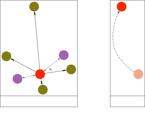
Figure 2: Description of a neighborhood of each $smart\_cell$ in the CCAA

Once the neighborhood has been generated, the best position with minimum cost is selected (Fig. 2 $(B)$) to upgrade the $smart\_cell$ if it improves its cost, or otherwise with a probability of $50\%$. The elitism of the CCAA serves to preserve the information of the best solutions generated by the optimization process. The probability of substituting a $smart\_cell$ for another with a worse value also helps the algorithm avoid stagnation at local minima. Figure 3 shows the CCAA flow chart.

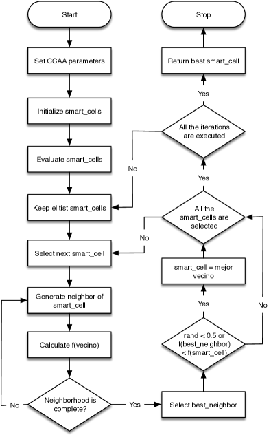
Figure 3: CCAA flow chart

4 Experimental results

To validate the effectiveness of the CCAA, $2$ groups of experiments with different types of functions were developed.

The first group evaluated the CCAA with $23$ scalable proof problems in $30$ dimensions and $10$ problems with fixed dimensions. The results are compared with $7$ other recently published meta-heuristics, namely, the CPSO (Shi et al., 2011), the gray wolf optimizer (GWO) (Mirjalili et al., 2014), the whale optimization algorithm (WOA) (Mirjalili and Lewis, 2016), the mayfly optimization algorithm (MA) (Zervoudakis and Tsafarakis, 2020), the adaptive logarithmic spiral-Levy firefly algorithm (ADIFA) (Wu et al., 2020), the double adaptive random spare reinforced whale optimization algorithm (Chen et al., 2020), and the modified sine cosine algorithm (MSCA) (Gupta et al., 2020). The test problems used have been widely utilized to validate the performances of various algorithms (Gupta et al., 2020) (Zervoudakis and Tsafarakis, 2020) (Chen et al., 2020) (Wu et al., 2020). Most of the codes for these algorithms were taken from the sites noted in the references, so these are mostly implementations made by the same authors of the indicated papers, which provide a more objective comparison between algorithms. The only algorithm implemented was the MSCA, for which the original SCA code was taken and modified following the instructions published in (Gupta et al., 2020).

The definitions of the test problems are presented in Tables 1, 2, and 3. Comparison with the other algorithms shows the average value and the standard deviation of their values obtained in the objective functions, taking $30$ independent runs of each algorithm. The second set of experiments contemplates the same $23$ scalable test problems but in $500$ dimensions, making the same statistical comparisons of the average and standard deviations in another $30$ independent runs for each algorithm. A comparative statistical analysis was performed in each set of experiments applying the Wilcoxon rank-sum test, also showing some convergence and box diagrams for selected functions.

A preliminary study was conducted that considered different values of the CCAA parameters and they were applied to the problems $F_{6}$, $F_{11}$, and $F_{24}$ in $30$ dimensions to select the best parameters. For the population size and the number of generations, $smart\_n=12$, $neighbor\_n=6$, and $iteration\_n=500$ were taken to have parameters similar to the algorithms used for comparison.

The other CCAA parameters were tested on two levels to choose the best combination. For $lower_{p}$, $0.5$ and $1$ were taken; for $upper_{p}$, $2$ and $3$ were tested. For $dist\_M$, $1$ and $2$ were analyzed; for $dist\_m$, the values $0.15$ and $0.3$ were verified. For $lower_{d}$, $0.5$ and $1$ were taken; for $upper_{d}$, $3$ and $4$ were tested; and for $elitism\_n$, the values $1$ and $2$ were studied; having a total of $128$ combinations. For each combination, $30$ independent runs of the CCAA were made in the three functions selected, and the combination of parameters that obtained the best average value was chosen. As a result of this analysis, the parameters selected to conduct the comparison of the CCAA with the other algorithms in the following experiments are $lower_{p}=1$, $upper_{p}=2$, $dist\_M=1$, $dist\_m=0.3$, $lower_{d}=1$, $upper_{d}=4$, and $elitism\_n=2$.

The CCAA was implemented in Matlab 2015a, on a machine with Intel Xeon CPU at $3.1$ GHz, $64$ GB in the RAM, and $1$ TB in the hard disk, running on Mac OS X Catalina operating system.

4.1 Experiment 1: Functions on $30$ dimensions and functions with fixed dimensions

This section compares the performance of the CCAA against 6 other recently published algorithms for global optimization, using $23$ scalable test functions that were tested in this experiment with $30$ dimensions and are described in Tables 1 and 2. The comparison with the other $10$ functions of fixed dimensions is also shown, which are defined in Table 3.

Table 1: Description of scalable-dimensional unimodal benchmark functions

Function	Dimensions	Range	$f_{min}$
$F1(x)=\sum_{i=1}^{n}x_{i}^{2}$	$30$, $500$	$[-100,100]$	$0$
$F2(x)=\sum_{i=1}^{n}ix_{i}^{2}$	$30$, $500$	$[-10,10]$	$0$
$F3(x)=\sum_{i=1}^{n}|x_{i}|+\prod_{i=1}^{n}|x_{i}|$	$30$, $500$	$[-10,10]$	$0$
$F4(x)=\sum_{i=1}^{n}\left(\sum_{j=1}^{i}x_{j}\right)^{2}$	$30$, $500$	$[-100,100]$	$0$
$F5(x)=\max_{i}\left\{|x_{i}|,1\leq i\leq n\right\}$	$30$, $500$	$[-100,100]$	$0$
$F6(x)=\sum_{i=1}^{n-1}\left(100\left(x_{i+1}-x_{i}^{2}\right)^{2}+(x_{i}-1)^{2}\right)$	$30$, $500$	$[-30,30]$	$0$
$F7(x)=\sum_{i=1}^{n}\left(x_{i}+0.5\right)^{2}$	$30$, $500$	$[-100,100]$	$0$
$F8(x)=\sum_{i=1}^{n}ix_{i}^{4}$	$30$, $500$	$[-1.28,1.28]$	$0$
$F9(x)=\sum_{i=1}^{n}ix_{i}^{4}+random[0,1)$	$30$, $500$	$[-1.28,1.28]$	$0$
$F10(x)=\sum_{i=1}^{n}|x_{i}|^{i+1}$	$30$, $500$	$[-1,1]$	$0$

The first $10$ test functions are unimodal and are useful in the evaluation of the exploitation properties of the $smart\_cells$ in the CCAA. The following $13$ test functions are multimodal and used to analyze the CCAA’s ability to explore and escape local minima. Lastly, the test functions with fixed dimensionality have a lower number of local minima and are useful in the observation of the balance between the exploration and exploitation actions of the CCAA.

In this experiment, $30$ independent runs were made per algorithm; for the CPSO and the CCAA, $smart\_n=12$ and $neighbor\_n=6$ were used; for the rest of the algorithms, $(smart\_n)(neighbor\_n)=72$ individuals were used. In all algorithms, $iteration\_n=500$ was employed. Table 4 presents the results of the comparison with respect to the average and standard deviation for the unimodal functions, Table 5 shows the same values for multimodal functions, and Table 6 presents the results for functions on fixed dimensions.

Table 2: Description of scalable-dimensional multimodal benchmark functions

Function	Dimensions	Range	$f_{min}$
$F11(x)=\sum_{i=1}^{n}-x_{i}sin\left(\sqrt{|x_{i}|}\right)$	$30$, $500$	$[-500,500]$	$-418.9829\times n$
$F12(x)=\sum_{i=1}^{n}\left(x_{i}^{2}-10cos(2\pi x_{i})+10\right)$	$30$, $500$	$[-5.12,5.12]$	$0$
$F13(x)=-20\exp\left(-0.2\sqrt{\frac{1}{n}\sum_{i=1}^{n}x_{i}^{2}}\right)$	$30$, $500$	$[-32,32]$	$0$
$-\exp\left(\frac{1}{n}\sum_{i=1}^{n}cos(2\pi x_{i})\right)+20+e$
$F14(x)=\frac{1}{4000}\sum_{i=1}^{n}x_{i}^{2}-\prod_{i=1}^{n}cos\left(\frac{x_{i}}{\sqrt{i}}\right)+1$	$30$, $500$	$[-600,600]$	$0$
$F15(x)=\frac{\pi}{n}\left(10sin(\pi y_{1})+\sum_{i=1}^{n-1}(y_{i}-1)^{2}\left(1+10sin^{2}(\pi y_{i+1})\right)\right.$	$30$, $500$	$[-50,50]$	$0$
$\left.+(y_{n}-1)^{2}\right)+\sum_{i=1}^{n}u(x_{i},10,100,4);\;y_{i}=1+\frac{x_{i}+1}{4};$
$u(x_{i},a,k,m)=\left\{\begin{array}[]{l}k(x_{i}-a)^{m},\;x_{i}>a\\ -a,\;-a\leq x_{i}\leq a\\ k(-x_{i}-a)^{m},\;x_{i}<-a\\ \end{array}\right.$
$F16(x)=0.1\left[sin^{2}(3\pi x_{1})+\sum_{i=1}^{n-1}(x_{i}-1)^{2}\left(1+sin^{2}(3\pi x_{i}+1)\right)\right.+$	$30$, $500$	$[-50,50]$	$0$
$\left.(x_{n}-1)^{2}\left(1+sin^{2}(2\pi x_{n})\right)\right]+\sum_{i=1}^{n}u(x_{i},5,100,4)$
$F17(x)=\sum_{i=1}^{n}|x_{i}sin(x_{i})+0.1x_{i}|$	$30$, $500$	$[-10,10]$	$0$
$F18(x)=\sum_{i=1}^{n}0.1n-\left(0.1\sum_{i=1}^{n}cos(5\pi x_{i})-\sum_{i=1}^{n}x_{i}^{2}\right)$	$30$, $500$	$[-1,1]$	$0$
$F19(x)=\sum_{i=1}^{n}\left(x_{i}^{2}+2x_{i+1}^{2}\right)^{0.25}\times\left(1+sin(50(x_{i}^{2}+x_{i+1}^{2})^{0.1}\right)^{2}$	$30$, $500$	$[-1.28,1.28]$	$0$
$F20(x)=\sum_{i=1}^{n}(10^{6})^{(i-1)/(n-1)}x_{i}^{2}$	$30$, $500$	$[-100,100]$	$0$
$F21(x)=(-1)^{n+1}\prod_{i=1}^{n}cos(x_{i})\times\exp\left(-\sum_{i=1}^{n}(x_{i}-\pi)^{2}\right)$	$30$, $500$	$[-100,100]$	$-1$
$F22(x)=1-cos\left(2\pi\sqrt{\left(\sum_{i=1}^{n}x_{i}^{2}\right)}\right)+0.1\sqrt{\left(\sum_{i=1}^{n}x_{i}^{2}\right)}$	$30$, $500$	$[-100,100]$	$0$
$F23(x)=0.5+\left(sin^{2}\left(\sqrt{\left(\sum_{i=1}^{n}x_{i}^{2}\right)}\right)-0.5\right)/\left(1+0.001\left(\sum_{i=1}^{n}x_{i}^{2}\right)^{2}\right)$	$30$, $500$	$[-100,100]$	$0$

Table 3: Description of fixed-dimension multimodal benchmark functions

Function	Dimensions	Range	$f_{min}$
$F24(x)=\left(\frac{1}{500}+\sum_{j=1}^{25}\frac{1}{j+\sum_{i=1}^{2}(x_{i}-a_{ij})^{6}}\right)^{-1}$	$2$	$[-65,65]$	$1$
$F25(x)=\sum_{i=1}^{11}\left(a_{i}-\frac{x_{1}(b_{i}^{2}+b_{i}x_{2})}{b_{i}^{2}+b_{i}x_{3}+x_{4}}\right)^{2}$	$4$	$[-5,5]$	$0.00030$
$F26(x)=4x_{1}^{2}-2.1x_{1}^{4}+(1/3)x_{1}^{6}+x_{1}x_{2}-4x_{2}^{2}+4x_{2}^{4}$	$2$	$[-5,5]$	$-1.0316$
$F27(x)=\left(x_{2}-(5.1/4\pi^{2})x_{1}^{2}+(5/\pi)x_{1}-6\right)^{2}+10(1-(1/8\pi))cos(x_{1})+10$	$2$	$[-5,5]$	$0.398$
$F28(x)=\left(1+(x_{1}+x_{2}+1)^{2}(19-14x_{1}+3x_{1}^{2}-14x_{2}+6x_{1}x_{2}+3x_{2}^{2})\right)$	$2$	$[-2,2]$	$3$
$\times\left(30+(2x_{1}-3x_{2})^{2}\times(18-32x_{1}+12x_{1}^{2}+48x_{2}-36x_{1}x_{2}+27x_{2}^{2})\right)$
$F29(x)=-\sum_{i=1}^{4}c_{i}\exp\left(-\sum_{j=1}^{3}a_{ij}(x_{j}-p_{ij})^{2}\right)$	$3$	$[1,3]$	$-3.86$
$F30(x)=-\sum_{i=1}^{4}c_{i}\exp\left(-\sum_{j=1}^{6}a_{ij}(x_{j}-p_{ij})^{2}\right)$	$6$	$[0,1]$	$-3.32$
$F31(x)=-\sum_{i=1}^{5}\left((X-a_{i})(X-a_{i})^{T}+c_{i}\right)^{-1}$	$4$	$[0,10]$	$-10.1532$
$F32(x)=-\sum_{i=1}^{7}\left((X-a_{i})(X-a_{i})^{T}+c_{i}\right)^{-1}$	$4$	$[0,10]$	$-10.4028$
$F33(x)=-\sum_{i=1}^{10}\left((X-a_{i})(X-a_{i})^{T}+c_{i}\right)^{-1}$	$4$	$[0,10]$	$-10.5363$

For unimodal problems, the CCAA obtained $9$ of the $10$ best results with respect to the average value; i.e., the CCAA was able to achieve the optimal solutions for the problems $F1$ to $F5$, $F7$, $F8$, and $F10$ . Furthermore, in $8$ of $10$ cases, the CCAA produced the best values concerning the standard deviation, which gives evidence of the proposed algorithm’s information exploitation capacity.

For the $13$ multimodal problems, the CCAA also obtained $9$ of the $13$ best average values,($F11$, $F13$ to $F16$ and from $F18$ to $F21$). In $5$ of them, the optimal values were calculated ($F11$, $F14$, and from $F18$ to $F20$). The performance of the CCAA is comparable to the MSCA, which produced $8$ better average values, where $7$ of them were optimal values. In $8$ out of $13$ cases, the CCAA achieved the best values referring to the standard deviation, showing the CCAA’s exploration ability.

For the $10$ fixed-dimension problems, the CCAA produced $7$ of the best average values ($F24$, $F27$ and from $F29$ to $F33$). Optimal value was reached in $6$ of them ($F27$ and from $F29$ to $F33$). The performance of the CCAA is comparable to the MA, which only got $5$ best average values, where $4$ of them are optimal values. In $5$ out of $10$ cases, the CCAA calculated the best values for the standard deviation, showing the robustness of the CCAA in carrying out exploration and exploitation actions simultaneously.

Table 4: Performance of meta-heuristic algorithms compared with the CCAA on 30-dimensional unimodal problems

Function	CPSO		GWO		WOA		MA		ADIFA		RDWOA		MSCA		CCAA
	mean	std	mean	std	mean	std	mean	std	mean	std	mean	std	mean	std	mean	std
F1	8.76e-07	1.32e-06	1.98e-37	2.33e-37	1.97e-89	1.39e-88	5.19e-07	8.70e-07	1.35e+03	4.09e+02	1.06e-141	4.37e-141	0.00e+00	0.00e+00	0.00e+00	0.00e+00
F2	4.00e+00	2.83e+01	3.45e-38	5.41e-38	1.86e-91	9.12e-91	9.35e-08	1.33e-07	6.26e+01	3.22e+01	1.42e-141	5.92e-141	0.00e+00	0.00e+00	0.00e+00	0.00e+00
F3	7.79e+00	1.17e+01	4.83e-22	3.40e-22	1.02e-55	4.97e-55	8.36e-05	3.79e-04	9.05e+00	3.37e+00	5.26e-88	1.75e-87	0.00e+00	0.00e+00	0.00e+00	0.00e+00
F4	5.60e+03	4.23e+03	4.14e-09	1.92e-08	1.92e+04	7.87e+03	5.96e+03	2.19e+03	1.89e+03	7.15e+02	3.56e-64	1.54e-64	0.00e+00	0.00e+00	0.00e+00	0.00e+00
F5	9.96e+00	5.31e+00	1.90e-09	2.87e-09	2.74e+01	3.08e+01	4.59e+01	8.64e+00	2.75e+01	6.59e+00	2.19e-39	3.98e-39	0.00e+00	0.00e+00	0.00e+00	0.00e+00
F6	1.84e+03	1.27e+04	2.67e+01	8.22e-01	2.71e+01	2.51e-01	6.88e+01	4.78e+01	9.07e+04	6.52e+04	2.34e+01	1.94e+00	9.61e+00	1.29e+01	1.03e+00	5.12e+00
F7	2.01e-06	7.56e-06	3.11e-01	2.82e-01	1.85e-02	2.62e-02	3.94e-07	5.11e-07	1.34e+03	4.58e+02	2.42e-01	2.37e-01	5.89e-08	1.02e-07	0.00e+00	0.00e+00
F8	6.20e-17	2.27e-16	4.48e-67	1.90e-66	2.54e-156	1.55e-155	7.12e-15	3.01e-14	2.81e-03	2.58e-03	5.28e-241	0.00e+00	0.00e+00	0.00e+00	0.00e+00	0.00e+00
F9	7.46e-02	8.96e-02	7.80e-04	6.06e-04	1.65e-03	1.85e-03	1.80e-02	5.81e-03	3.78e-01	1.80e-01	5.64e-05	5.07e-05	3.91e-05	4.02e-05	2.36e-04	1.94e-04
F10	3.80e-01	5.67e-01	3.31e-23	2.07e-23	4.79e-56	3.28e-55	4.71e-06	1.02e-05	7.27e-01	2.43e-01	5.94e-89	1.68e-88	0.00e+00	0.00e+00	0.00e+00	0.00e+00

Table 5: Performance of meta-heuristic algorithms compared with the CCAA on 30-dimensional multimodal problems

Function	CPSO		GWO		WOA		MA		ADIFA		RDWOA		MSCA		CCAA
	mean	std	mean	std	mean	std	mean	std	mean	std	mean	std	mean	std	mean	std
F11	-9.97e+03	6.28e+02	-6.41e+03	7.13e+02	-1.14e+04	1.36e+03	-1.00e+04	4.26e+02	-6.68e+03	8.05e+02	-8.88e+03	6.77e+02	-1.26e+04	6.70e-03	-1.26e+04	7.35e-12
F12	1.63e+02	4.58e+01	1.58e+00	3.07e+00	0.00e+00	0.00e+00	2.58e+01	1.03e+01	5.34e+01	1.93e+01	0.00e+00	0.00e+00	0.00e+00	0.00e+00	1.19e+00	5.91e+00
F13	1.82e+01	5.19e+00	3.31e-14	4.21e-15	4.58e-15	2.87e-15	1.57e+00	5.35e-01	8.40e+00	1.66e+00	4.16e-15	9.74e-16	8.88e-16	0.00e+00	8.88e-16	0.00e+00
F14	1.27e-02	1.97e-02	1.79e-03	5.10e-03	5.66e-03	1.76e-02	1.79e-02	2.21e-02	1.59e+01	4.34e+00	8.87e-04	3.14e-03	0.00e+00	0.00e+00	0.00e+00	0.00e+00
F15	2.90e-02	1.26e-01	2.12e-02	1.31e-02	3.68e-03	6.15e-03	4.15e-01	6.18e-01	1.42e+01	8.97e+00	6.86e-03	6.06e-03	8.96e-09	2.19e-08	1.57e-32	5.53e-48
F16	3.32e-01	1.28e+00	2.51e-01	1.54e-01	8.23e-02	7.16e-02	2.25e-01	3.88e-01	5.17e+03	1.09e+04	2.51e-01	1.50e-01	5.93e-02	4.19e-01	1.35e-32	1.11e-47
F17	3.11e-03	9.76e-03	2.85e-04	5.02e-04	2.77e-41	1.96e-40	1.04e-05	2.64e-05	3.12e+00	1.60e+00	1.97e-12	9.32e-12	9.78e-08	6.92e-07	1.25e-11	5.52e-11
F18	1.02e+00	3.68e-01	0.00e+00	0.00e+00	0.00e+00	0.00e+00	9.46e-02	1.15e-01	9.64e-01	3.33e-01	0.00e+00	0.00e+00	0.00e+00	0.00e+00	0.00e+00	0.00e+00
F19	2.37e+01	1.31e+01	1.15e-10	4.57e-11	1.53e-31	5.45e-31	2.52e-02	1.64e-02	4.07e+01	7.30e+00	9.07e-46	2.71e-45	0.00e+00	0.00e+00	0.00e+00	0.00e+00
F20	1.34e+06	1.88e+06	4.69e-34	6.10e-34	1.03e-87	5.80e-87	1.29e+00	8.21e+00	1.27e+07	6.98e+06	3.73e-138	2.48e-137	0.00e+00	0.00e+00	0.00e+00	0.00e+00
F21	0.00e+00	0.00e+00	0.00e+00	0.00e+00	0.00e+00	0.00e+00	0.00e+00	0.00e+00	0.00e+00	0.00e+00	0.00e+00	0.00e+00	0.00e+00	0.00e+00	-7.00e-01	4.63e-01
F22	1.77e+00	1.31e+00	1.76e-01	4.31e-02	1.42e-01	7.02e-02	1.34e+00	5.42e-01	4.43e+00	6.56e-01	9.39e-02	2.40e-02	0.00e+00	0.00e+00	7.79e-02	4.18e-02
F23	4.97e-01	8.40e-03	1.00e-01	1.08e-01	1.19e-01	1.27e-01	4.99e-01	1.55e-03	5.00e-01	1.17e-03	4.19e-02	8.64e-03	0.00e+00	0.00e+00	2.97e-02	2.06e-02

Table 6: Performance of meta-heuristic algorithms compared with the CCAA on fixed-dimensional problems

Function	CPSO		GWO		WOA		MA		ADIFA		RDWOA		MSCA		CCAA
	mean	std	mean	std	mean	std	mean	std	mean	std	mean	std	mean	std	mean	std
F24	1.02e+00	1.41e-01	3.00e+00	3.29e+00	1.85e+00	2.00e+00	9.98e-01	0.00e+00	1.06e+00	2.38e-01	2.41e+00	3.30e+00	9.98e-01	3.57e-11	9.98e-01	1.31e-16
F25	7.24e-03	1.14e-02	1.99e-03	5.48e-03	6.37e-04	2.69e-04	1.20e-03	3.96e-03	7.03e-04	4.35e-04	2.00e-03	1.19e-02	3.59e-04	1.83e-04	7.93e-04	2.84e-03
F26	-1.03e+00	2.37e-16	-1.03e+00	9.79e-09	-1.03e+00	7.14e-11	-1.03e+00	2.24e-16	-1.03e+00	1.33e-11	-1.03e+00	5.60e-16	-1.03e+00	2.00e-06	-1.03e+00	1.41e-14
F27	3.98e-01	3.36e-16	3.98e-01	3.78e-07	3.98e-01	3.12e-07	3.98e-01	3.36e-16	3.98e-01	3.43e-12	3.98e-01	6.04e-16	3.98e-01	3.56e-05	3.98e-01	3.36e-16
F28	3.00e+00	7.59e-16	3.00e+00	8.24e-06	3.00e+00	1.23e-05	3.00e+00	3.42e-15	3.00e+00	6.93e-10	3.00e+00	1.24e-12	3.00e+00	2.30e-06	4.08e+00	5.34e+00
F29	-3.86e+00	3.14e-15	-3.86e+00	2.15e-03	-3.86e+00	2.20e-03	-3.86e+00	3.14e-15	-3.86e+00	1.43e-09	-3.86e+00	2.49e-15	-3.86e+00	3.71e-03	-3.86e+00	2.59e-15
F30	-3.28e+00	5.60e-02	-3.25e+00	7.83e-02	-3.24e+00	9.09e-02	-3.28e+00	5.83e-02	-3.23e+00	5.13e-02	-3.27e+00	5.99e-02	-3.13e+00	1.12e-01	-3.32e+00	1.70e-09
F31	-9.13e+00	2.06e+00	-9.75e+00	1.38e+00	-9.48e+00	1.83e+00	-6.25e+00	3.58e+00	-8.85e+00	2.18e+00	-9.24e+00	1.98e+00	-1.02e+01	1.26e-04	-1.02e+01	5.45e-12
F32	-9.23e+00	2.22e+00	-1.03e+01	7.52e-01	-9.16e+00	2.39e+00	-7.04e+00	3.57e+00	-9.32e+00	2.14e+00	-8.38e+00	2.61e+00	-1.04e+01	1.92e-04	-1.04e+01	3.06e-12
F33	-1.01e+01	1.48e+00	-1.01e+01	1.76e+00	-8.90e+00	2.83e+00	-7.58e+00	3.53e+00	-9.65e+00	2.07e+00	-8.70e+00	2.59e+00	-1.05e+01	1.05e-04	-1.05e+01	1.33e-12

Table 7 presents the results on the range that each algorithm obtained with respect to its average value in each test problem, for $30$ dimensions and the functions with fixed dimension, as well as the results of the Wilcoxon rank-sum test to compare the CCAA with the other algorithms for each test function. Use of the $+$ symbol indicates that the CCAA obtained a significantly better statistical result than the other algorithm, a $-$ symbol indicates a significantly worse statistical result, and the $\ approx$ symbol indicates no statistically significant difference. The penultimate row shows each algorithm’s average rank and the difference between the number of positive tests ($+$) minus the number of negative tests ($-$), where a positive value indicates that the CCAA obtained a more significant number of positive statistical tests against the reference algorithm. Finally, the last row indicates each algorithm’s rank with regard to the average range of the $33$ test problems.

In Table 7, the CCAA always achieved a favorable comparison against the other algorithms for the Wilcoxon rank-sum test and its average rank is the best ($1.55$), followed closely by the MSCA ($2.15$). These results show the excellent overall effectiveness of the CCAA for problems in $30$ dimensions and with fixed dimensions.

Table 7: Results of the Wilcoxon rank-sum test and ranking of all the compared algorithms on $30$-dimensional and fixed-dimensional problems

Function	CPSO		GWO		WOA		MA		ADIFA		RDWOA		MSCA		MSCA
	Rank	Test	Rank	Test	Rank	Test	Rank	Test	Rank	Test	Rank	Test	Rank	Test	Rank
F1	6	+	4	+	3	+	5	+	7	+	2	+	1	$\approx$	1
F2	6	+	4	+	3	+	5	+	7	+	2	+	1	$\approx$	1
F3	6	+	4	+	3	+	5	+	7	+	2	+	1	$\approx$	1
F4	5	+	3	+	7	+	6	+	4	+	2	+	1	$\approx$	1
F5	4	+	3	+	5	+	7	+	6	+	2	+	1	$\approx$	1
F6	7	+	4	+	5	+	6	+	8	+	3	+	2	+	1
F7	4	+	7	+	5	+	3	+	8	+	6	+	2	+	1
F8	5	+	4	+	3	+	6	+	7	+	2	+	1	$\approx$	1
F9	7	+	4	+	5	+	6	+	8	+	2	-	1	-	3
F10	6	+	4	+	3	+	5	+	7	+	2	+	1	$\approx$	1
F11	5	+	8	+	3	+	4	+	7	+	6	+	2	+	1
F12	6	+	3	+	1	$\approx$	4	+	5	+	1	$\approx$	1	$\approx$	2
F13	7	+	4	+	3	+	5	+	6	+	2	+	1	$\approx$	1
F14	5	+	3	+	4	+	6	+	7	+	2	+	1	$\approx$	1
F15	6	+	5	+	3	+	7	+	8	+	4	+	2	+	1
F16	7	+	6	+	3	+	4	+	8	+	5	+	2	+	1
F17	7	+	6	+	1	-	5	+	8	+	2	-	4	$\approx$	3
F18	4	+	1	$\approx$	1	$\approx$	2	+	3	+	1	$\approx$	1	$\approx$	1
F19	6	+	4	+	3	+	5	+	7	+	2	+	1	$\approx$	1
F20	6	+	4	+	3	+	5	+	7	+	2	+	1	$\approx$	1
F21	2	+	2	+	2	+	2	+	2	+	2	+	2	+	1
F22	7	+	5	+	4	$\approx$	6	+	8	+	3	+	1	-	2
F23	6	+	4	+	5	$\approx$	7	+	8	+	3	+	1	-	2
F24	3	+	7	+	5	+	1	$\approx$	4	+	6	+	2	+	1
F25	8	$\approx$	6	+	2	-	5	+	3	-	7	+	1	-	4
F26	1	-	5	+	4	+	1	-	3	+	1	$\approx$	6	+	2
F27	1	$\approx$	5	+	4	+	1	$\approx$	3	+	2	+	6	+	1
F28	2	-	7	-	6	-	1	-	4	-	3	$\approx$	5	-	8
F29	1	$\approx$	3	+	4	+	1	$\approx$	2	+	1	$\approx$	5	+	1
F30	2	+	5	+	6	+	3	+	7	+	4	$\approx$	8	+	1
F31	6	+	3	+	4	+	8	$\approx$	7	+	5	+	2	+	1
F32	5	+	3	+	6	+	8	$\approx$	4	+	7	$\approx$	2	+	1
F33	3	+	4	+	6	+	8	$\approx$	5	+	7	$\approx$	2	+	1
Avg. & WRST	4.91	26	4.36	30	3.79	23	4.64	23	5.91	29	3.12	21	2.15	9	1.55
Overall rank	7		5		4		6		8		3		2		1

Figure 4 presents a sample of the convergence curves of the algorithms used in this experiment for different test problems. Figure 5 shows the box plots for the algorithms that obtained the best results in the test problems described in Fig. 4.

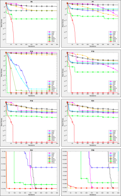
Figure 4: Convergence curves of the different algorithms for test functions in $30$ dimensions

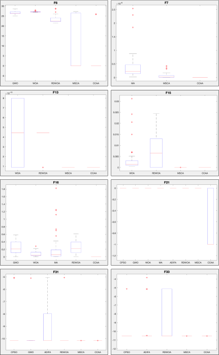
Figure 5: Box plots with the best results of different algorithms for test functions in $30$ dimensions

4.2 Experiment 2: Functions on $500$ dimensions and functions with fixed dimensions

This section compares the performance of the CCAA against the $6$other algorithms for the $23$ scalable test functions using $500$ dimensions. A new comparison with the $10$ fixed-dimension functions is also shown to result in findings similar to the first one.

There were $30$ independent runs per algorithm in this case as well; for the CPSO and the CCAA, $smart\_n=12$ and $neighbor\_n=6$ were used; for the rest of the algorithms, $(smart\_n)(neighbor\_n)=72$ individuals were applied. In all algorithms, $iteration\_n=500$ was employed. Table 8 presents the results of the comparison with respect to the mean and standard deviation for the unimodal functions, Table 9 shows the same comparison for multimodal functions, and Table 10 describes the results for functions with fixed dimensions.

For unimodal problems, the CCAA obtains $8$ of the $10$ best average values, i.e., the CCAA was able to obtain optimal solutions for $F1$ to $F3$, $F5$, $F7$, $F8$, and $F10$. Moreover, in $7$ out of $10$ cases, the CCAA achieved the best values concerning the standard deviation, which again gives evidence of its exploitation capacity.

For the $13$ multimodal problems, the CCAA also produced $10$ of the $13$ best average values in the functions $F11$ to $F16$ and from $F18$ to $F21$. In $7$ of them ($F11$, $F12$, $F14$, and from $F18$ to $F21$), the optimal values were calculated. The performance of the CCAA is comparable with that of the MSCA, which obtains $9$ better average values, with $8$ of them were optimal values. In $9$ out of $13$ cases, the CCAA achieved the best values referring to the standard deviation, which also shows the CCAA’s exploration ability.

For the second run with $10$ fixed-dimension test functions, the CCAA produced $6$ of the best average values for the functions of $F27$ and from $F29$ to $F33$. In all of them, the CCAA obtained the optimal values. The performance of the CCAA is comparable to that of the MA, which produced $5$ better average values, where again $4$ were optimal values. For this experiment, the CCAA reached the lowest value in $6$ of $10$ cases for the standard deviation, showing once again the robustness of the CCAA to carry out exploration and exploitation actions in a balanced way.

Table 11 presents the results on the range that each algorithm obtained with respect to its average value in each test problem, for $500$ dimensions and functions with fixed dimension, as well as the results of the Wilcoxon rank-sum test to compare the CCAA with the other algorithms for each test function. In Table 11, the CCAA always has a favorable comparison versus the other algorithms concerning the Wilcoxon rank-sum test and its average rank is the best ($1.45$), followed again by the MSCA ($2.21$). These results show how effective the CCAA is in general for problems with $500$ and fixed dimensions.

Table 8: Performance of meta-heuristic algorithms compared with the CCAA on 500-dimensional unimodal problems

Function	CPSO		GWO		WOA		MA		ADIFA		RDWOA		MSCA		CCAA
	mean	std	mean	std	mean	std	mean	std	mean	std	mean	std	mean	std	mean	std
F1	5.01e+05	1.15e+05	3.99e-05	1.39e-05	1.19e-84	8.36e-84	9.74e+05	1.25e+05	5.96e+04	9.37e+03	3.29e-81	4.91e-81	0.00e+00	0.00e+00	0.00e+00	0.00e+00
F2	1.13e+06	2.17e+05	7.18e-05	2.93e-05	3.37e-87	1.95e-86	1.56e+06	1.22e+05	1.73e+05	2.56e+04	6.49e-81	1.13e-80	0.00e+00	0.00e+00	0.00e+00	0.00e+00
F3	1.32e+03	3.73e+02	1.33e-03	2.34e-04	4.60e-54	1.78e-53	3.83e+50	2.65e+51	9.34e+12	6.60e+13	8.32e-55	2.16e-54	0.00e+00	0.00e+00	0.00e+00	0.00e+00
F4	3.23e+06	5.09e+05	1.87e+05	5.74e+04	2.60e+07	7.06e+06	3.99e+06	5.39e+05	6.03e+05	1.97e+05	7.50e-61	1.53e-61	0.00e+00	0.00e+00	3.08e-07	1.71e-06
F5	6.50e+01	6.09e+00	5.64e+01	6.23e+00	7.03e+01	2.86e+01	9.91e+01	1.86e-01	5.54e+01	6.73e+00	2.92e-32	6.61e-34	0.00e+00	0.00e+00	0.00e+00	0.00e+00
F6	1.09e+09	3.42e+08	4.97e+02	2.83e-01	4.95e+02	1.91e-01	7.10e+09	1.95e+08	1.60e+07	4.92e+06	4.95e+02	1.05e+00	1.88e+02	2.42e+02	9.86e+00	6.97e+01
F7	4.69e+05	9.99e+04	8.34e+01	1.95e+00	1.19e+01	2.74e+00	9.40e+05	1.04e+05	6.10e+04	9.37e+03	5.43e+01	4.04e+00	1.93e-06	5.98e-06	0.00e+00	0.00e+00
F8	7.61e+03	1.81e+03	7.45e-13	6.07e-13	2.13e-147	1.14e-146	5.39e+04	1.10e+04	1.59e+02	4.60e+01	7.55e-142	9.39e-142	0.00e+00	0.00e+00	0.00e+00	0.00e+00
F9	7.32e+03	3.02e+03	2.15e-02	5.44e-03	2.56e-03	3.60e-03	5.15e+04	1.28e+04	1.51e+02	4.27e+01	5.92e-05	5.53e-05	4.19e-05	4.77e-05	2.24e-04	1.53e-04
F10	1.30e+02	1.58e+01	1.47e-04	1.75e-05	4.20e-54	2.09e-53	7.97e+01	7.49e+00	5.12e+01	4.08e+00	1.39e-55	3.82e-55	0.00e+00	0.00e+00	0.00e+00	0.00e+00

Table 9: Performance of meta-heuristic algorithms compared with the CCAA on 500-dimensional multimodal problems

Function	CPSO		GWO		WOA		MA		ADIFA		RDWOA		MSCA		CCAA
	mean	std	mean	std	mean	std	mean	std	mean	std	mean	std	mean	std	mean	std
F11	-8.93e+04	3.14e+03	-6.26e+04	8.10e+03	-1.89e+05	2.54e+04	-8.40e+04	4.76e+03	-3.42e+04	3.40e+03	-1.15e+05	1.34e+04	-2.09e+05	1.63e-01	-2.09e+05	1.18e-10
F12	5.61e+03	5.67e+02	4.67e+01	1.51e+01	1.82e-14	1.29e-13	4.91e+03	2.79e+02	3.62e+03	5.51e+02	0.00e+00	0.00e+00	0.00e+00	0.00e+00	0.00e+00	0.00e+00
F13	2.00e+01	2.65e-04	2.94e-04	5.47e-05	4.37e-15	2.64e-15	2.04e+01	3.40e-01	1.26e+01	1.04e+00	4.37e-15	5.02e-16	8.88e-16	0.00e+00	8.88e-16	0.00e+00
F14	4.59e+03	8.43e+02	2.94e-03	1.05e-02	0.00e+00	0.00e+00	9.02e+03	1.21e+03	4.63e+02	7.61e+01	0.00e+00	0.00e+00	0.00e+00	0.00e+00	0.00e+00	0.00e+00
F15	1.68e+09	7.08e+08	6.57e-01	3.33e-02	1.96e-02	6.25e-03	1.76e+10	5.16e+08	7.05e+04	1.01e+05	2.24e-01	3.17e-02	1.39e-09	1.66e-09	9.42e-34	6.91e-49
F16	4.18e+09	1.48e+09	4.65e+01	1.19e+00	5.76e+00	1.74e+00	3.19e+10	1.08e+09	1.03e+07	6.89e+06	3.15e+01	1.34e+00	9.89e-01	6.99e+00	1.35e-32	1.11e-47
F17	6.19e+02	6.20e+01	4.00e-02	5.98e-03	2.19e-53	1.22e-52	5.06e+02	5.62e+01	3.57e+02	3.88e+01	2.98e-14	1.77e-13	0.00e+00	0.00e+00	6.08e-12	3.76e-11
F18	1.02e+02	1.08e+01	3.06e-08	1.01e-08	0.00e+00	0.00e+00	1.56e+02	4.44e+01	4.83e+01	5.41e+00	0.00e+00	0.00e+00	0.00e+00	0.00e+00	0.00e+00	0.00e+00
F19	1.84e+03	9.99e+01	7.96e-01	6.42e-02	1.36e-30	5.53e-30	1.80e+03	3.86e+01	1.27e+03	7.13e+01	2.63e-32	5.59e-32	0.00e+00	0.00e+00	0.00e+00	0.00e+00
F20	1.12e+10	3.10e+09	6.53e-02	1.99e-02	7.39e-82	4.79e-81	8.11e+09	1.22e+09	3.41e+09	6.40e+08	6.61e-78	1.71e-77	0.00e+00	0.00e+00	0.00e+00	0.00e+00
F21	0.00e+00	0.00e+00	0.00e+00	0.00e+00	0.00e+00	0.00e+00	0.00e+00	0.00e+00	0.00e+00	0.00e+00	0.00e+00	0.00e+00	0.00e+00	0.00e+00	-2.60e-01	4.43e-01
F22	8.98e+01	4.86e+00	8.18e-01	8.50e-02	1.26e-01	6.94e-02	1.07e+02	3.27e+00	2.47e+01	1.97e+00	8.79e-02	3.28e-02	0.00e+00	0.00e+00	1.80e-02	3.88e-02
F23	5.00e-01	4.86e-11	4.97e-01	1.42e-03	1.00e-01	1.08e-01	5.00e-01	1.75e-11	5.00e-01	6.97e-08	4.19e-02	8.64e-03	0.00e+00	0.00e+00	7.86e-03	1.69e-02

Table 10: Performance of meta-heuristic algorithms compared with the CCAA on fixed-dimensional problems

Function	CPSO		GWO		WOA		MA		ADIFA		RDWOA		MSCA		CCAA
	mean	std	mean	std	mean	std	mean	std	mean	std	mean	std	mean	std	mean	std
F24	1.04e+00	1.97e-01	2.68e+00	3.25e+00	1.34e+00	7.12e-01	9.98e-01	4.49e-17	1.06e+00	3.11e-01	2.53e+00	3.04e+00	1.23e+00	1.65e+00	1.06e+00	3.11e-01
F25	8.44e-03	9.84e-03	2.35e-03	6.07e-03	7.52e-04	5.06e-04	1.21e-03	3.96e-03	9.00e-04	4.21e-04	3.28e-04	1.30e-04	3.64e-04	1.90e-04	3.62e-04	2.20e-04
F26	-1.03e+00	2.24e-16	-1.03e+00	8.63e-09	-1.03e+00	6.09e-11	-1.03e+00	2.24e-16	-1.03e+00	8.45e-12	-1.03e+00	5.74e-16	-1.03e+00	1.21e-06	-1.03e+00	4.51e-13
F27	3.98e-01	3.36e-16	3.98e-01	2.87e-07	3.98e-01	3.35e-07	3.98e-01	3.36e-16	3.98e-01	5.24e-12	3.98e-01	4.60e-16	3.98e-01	4.03e-05	3.98e-01	3.36e-16
F28	3.00e+00	1.76e-15	3.00e+00	7.63e-06	3.00e+00	7.48e-06	3.00e+00	3.56e-15	3.00e+00	5.59e-10	3.54e+00	3.82e+00	3.00e+00	1.32e-06	3.00e+00	1.47e-14
F29	-3.86e+00	3.14e-15	-3.86e+00	2.04e-03	-3.86e+00	1.88e-03	-3.86e+00	3.14e-15	-3.86e+00	2.39e-09	-3.86e+00	1.11e-03	-3.86e+00	3.84e-03	-3.86e+00	2.60e-15
F30	-3.27e+00	5.96e-02	-3.23e+00	7.11e-02	-3.24e+00	7.53e-02	-3.27e+00	5.88e-02	-3.23e+00	5.27e-02	-3.26e+00	6.00e-02	-3.18e+00	9.47e-02	-3.32e+00	1.68e-02
F31	-9.24e+00	1.98e+00	-9.55e+00	1.66e+00	-8.73e+00	2.62e+00	-6.75e+00	3.63e+00	-8.98e+00	2.12e+00	-8.52e+00	2.40e+00	-1.02e+01	1.90e-04	-1.02e+01	1.01e-11
F32	-9.49e+00	2.16e+00	-1.02e+01	1.04e+00	-9.13e+00	2.45e+00	-7.07e+00	3.66e+00	-8.99e+00	2.41e+00	-8.06e+00	2.67e+00	-1.04e+01	9.64e-05	-1.04e+01	4.60e-13
F33	-9.67e+00	2.00e+00	-1.05e+01	7.14e-04	-8.91e+00	2.66e+00	-7.66e+00	3.73e+00	-9.30e+00	2.37e+00	-8.37e+00	2.68e+00	-1.05e+01	1.22e-04	-1.05e+01	2.14e-12

Table 11: Results of the Wilcoxon rank-sum test and ranking of all the compared algorithms on $500$-dimensional and fixed-dimensional problems.

Function	CPSO		GWO		WOA		MA		ADIFA		RDWOA		MSCA		MSCA
	Rank	Test	Rank	Test	Rank	Test	Rank	Test	Rank	Test	Rank	Test	Rank	Test	Rank
F1	6	+	4	+	2	+	7	+	5	+	3	+	1	$\approx$	1
F2	6	+	4	+	2	+	7	+	5	+	3	+	1	$\approx$	1
F3	5	+	4	+	3	+	7	+	6	+	2	+	1	$\approx$	1
F4	6	+	4	+	8	+	7	+	5	+	2	$\approx$	1	-	3
F5	5	+	4	+	6	+	7	+	3	+	2	+	1	$\approx$	1
F6	7	+	5	+	3	+	8	+	6	+	4	+	2	+	1
F7	7	+	5	+	3	+	8	+	6	+	4	+	2	+	1
F8	6	+	4	+	2	+	7	+	5	+	3	+	1	$\approx$	1
F9	7	+	5	+	4	+	8	+	6	+	2	-	1	-	3
F10	7	+	4	+	3	+	6	+	5	+	2	+	1	$\approx$	1
F11	5	+	7	+	3	+	6	+	8	+	4	+	2	+	1
F12	6	+	3	+	2	$\approx$	5	+	4	+	1	$\approx$	1	$\approx$	1
F13	5	+	3	+	2	+	6	+	4	+	2	+	1	$\approx$	1
F14	4	+	2	+	1	$\approx$	5	+	3	+	1	$\approx$	1	$\approx$	1
F15	7	+	5	+	3	+	8	+	6	+	4	+	2	+	1
F16	7	+	5	+	3	+	8	+	6	+	4	+	2	+	1
F17	8	+	5	+	2	-	7	+	6	+	3	-	1	$\approx$	4
F18	4	+	2	+	1	$\approx$	5	+	3	+	1	$\approx$	1	$\approx$	1
F19	7	+	4	+	3	+	6	+	5	+	2	+	1	$\approx$	1
F20	7	+	4	+	2	+	6	+	5	+	3	+	1	$\approx$	1
F21	2	+	2	+	2	+	2	+	2	+	2	+	2	+	1
F22	7	+	5	+	4	+	8	+	6	+	3	+	1	-	2
F23	7	+	5	+	4	+	8	+	6	+	3	+	1	-	2
F24	2	-	7	+	5	+	1	-	3	$\approx$	6	+	4	+	3
F25	8	$\approx$	7	+	4	+	6	+	5	+	1	-	3	+	2
F26	1	-	5	+	4	+	1	-	3	+	1	$\approx$	6	+	2
F27	1	$\approx$	5	+	4	+	1	$\approx$	3	+	2	$\approx$	6	+	1
F28	2	-	7	+	6	+	1	-	4	+	8	+	5	+	3
F29	1	$\approx$	4	+	5	+	1	$\approx$	2	+	3	+	6	+	1
F30	3	$\approx$	7	+	5	+	2	$\approx$	6	+	4	$\approx$	8	+	1
F31	4	+	3	+	6	+	8	$\approx$	5	+	7	$\approx$	2	+	1
F32	4	+	3	+	5	+	8	$\approx$	6	+	7	$\approx$	2	+	1
F33	4	+	3	+	6	+	8	+	5	+	7	$\approx$	2	+	1
Avg. & WRST	5.09	23	4.42	33	3.58	28	5.73	22	4.79	32	3.21	17	2.21	12	1.45
Overall rank	7		5		4		8		6		3		2		1

Figure 6 presents a sample of the convergence curves of the algorithms used in this experiment for different test problems. Fig. 7 shows the box plots for the algorithms that obtained the best results in the test problems described in Fig. 6.

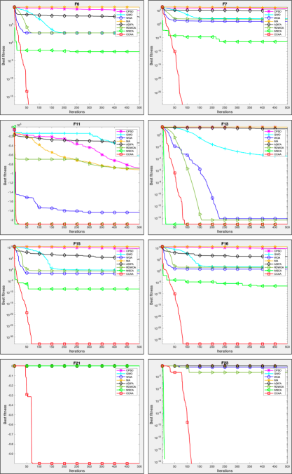
Figure 6: Convergence curves of the different algorithms for problems in $500$ dimensions

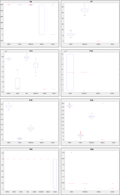
Figure 7: Box plots with the best results of different algorithms for problems in $500$ dimensions

4.3 Analysis of convergence behavior

In the computational experiments developed, it was observed that $smart\_cells$ tended to search extensively for optimal regions of the design space and exploit them concurrently. The $smart\_cells$ change abruptly in the early stages of the optimization process and then gradually converge. Such behavior can ensure that a population-based algorithm will eventually converge (Van Den Bergh and Engelbrecht, 2006). The convergence curves are compared in Figs. 4 and 6 for some of the problems. In these results, it can be observed that the CCAA is competitive with other recently proposed meta-heuristic algorithms.

The convergence curves of the CCAA show that its convergence tends to accelerate during the initial iterations of the optimization process. This convergence is due to the neighborhood mechanism and the different evolution rules that the $smart\_cells$ follow which help find promising regions of the search space and exploit them concurrently. Some evolution rules focus on exploration and others on exploitation, which produces an adequate balance to find the global optimum. In general, the experimental success rate of the CCAA algorithm is high as seen in Tables 7 and 11.

In summary, the high exploration capacity is due to the mechanism for updating the position of the $smart\_cells$ using the rules derived from the algorithms 1, 2 and 3. Simultaneously, the exploitation and convergence is performed using the different versions of the rules that are described in the algorithms 2, 4, 5 and 6. These rules allow $smart\_cells$ to rapidly relocate themselves to improve their position by exchanging information and using their own values. Since these rules are applied concurrently, the CCAA shows a high speed to avoid converging to local optima. The following sections verify the performance of the CCAA in engineering problems.

4.4 Engineering design problems

In engineering, there are many problems where mathematical models are applied that are later optimized. To show the utility of the CCAA in these cases, this section tests for $4$ design problems: a gear train, a pressure vessel, a welded beam, and a cantilever beam.

Given that these problems have different restrictions, the cost function is penalizing with an additional extra-large cost (because they are minimization problems) if one of the restrictions is not fulfilled. This objective function increment is simple to implement and has a low computational cost (Mirjalili and Lewis, 2016).

4.4.1 Gear train design (GTD)

The GTD problem was defined in (Sandgren, 1990) and has no restrictions other than being discrete and that each parameter is within a possible range of values. In this problem, we have $4$ decision parameters, $y_{1}$, $y_{2}$, $y_{3}$, and $y_{4}$, which represent the number of teeth that a gear can have (Fig. 8).

Figure 8: Gear train

The goal of this problem is to determine the minimum cost of gear ratio that can be set as follows:

$$min\;F(y_{1},y_{2},y_{3},y_{4})=\left(\frac{1}{6.931}-\frac{y_{2}y_{3}}{y_{1}y_{4}}\right)^{2}$$ (1)

where $12\leq y_{i}\leq 60$ for $i=(1,2,3,4)$ and each $y_{i}$ must be integer.

For this case, the result obtained by the CCAA is compared with the results published in (Gupta et al., 2020), which takes $17$ different meta-heuristic algorithms. Fifty independent runs of the CCAA were made and the best result was taken. In each run, $5$ $smart\_cells$ and $4$ neighbors were used for each $smart\_cell$, in addition to $200$ evaluations of $F$ to make the setting of the experiment similar to that of the one reported in (Gupta et al., 2020).

The reference values and the best design obtained by the CCAA are shown in Table 12. It can be seen that the CCAA obtained a design with a similar cost to the MSCA and the FA and a better result compared to the other algorithms. These outcomes show that the CCAA is competitive with the best algorithms for this discrete design problem.

Table 12: Comparison of meta-heuristics for the GTD problem

Algorithm	$y_{1}$	$y_{2}$	$y_{3}$	$y_{4}$	$F_{min}$
CCAA	$49$	$19$	$16$	$43$	$2.7009e-12$
MSCA	$49$	$16$	$19$	$43$	$2.7009e-12$
FA	$43$	$19$	$16$	$49$	$2.7009e-12$
m-SCA	$34$	$20$	$13$	$53$	$2.3078e-11$
TLBO	$53$	$30$	$13$	$51$	$2.3078e-11$
SCA-GWO	$51$	$26$	$15$	$53$	$2.3078e-11$
CMA-ES	$53$	$13$	$20$	$34$	$2.3078e-11$
wPSO	$57$	$12$	$37$	$54$	$8.8876e-10$
ISCA	$46$	$26$	$12$	$47$	$9.9216e-10$
PSO	$47$	$13$	$12$	$23$	$9.9216e-10$
GWO	$23$	$13$	$12$	$47$	$9.9216e-10$
SCA-PSO	$46$	$24$	$13$	$47$	$9.9216e-10$
SCA	$60$	$17$	$28$	$55$	$1.3616e-09$
SinDE	$30$	$17$	$14$	$55$	$1.3616e-09$
modSCA	$60$	$18$	$25$	$52$	$2.3576e-09$
SSA	$57$	$27$	$17$	$60$	$3.6358e-09$
OBSCA	$43$	$12$	$31$	$60$	$8.7008e-09$

4.4.2 Pressure vessel design (PVD)

For this problem, a mathematical model calculates the total cost of a cylindrical pressure vessel, showing the cost relationships concerning the material, the structure, and the weld. The design variables to specify are the thickness of the hull ($y_{1}$) and the head ($y_{2}$), the radius of the vessel ($y_{3}$), and the length of the vessel without counting the head ($y_{4}$), to minimize the total cost of the design (Gandomi et al., 2013). The cost function and its restrictions are shown in Eq. 2.

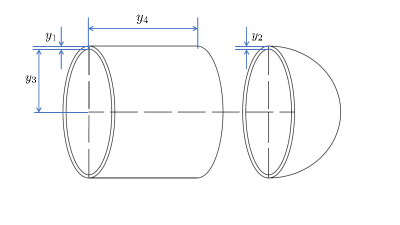
Figure 9: Pressure vessel

$$\begin{array}[]{l}min\;F(y_{1},y_{2},y_{3},y_{4})=0.6224y_{1}y_{3}y_{4}+1.7781y_{1}^{2}y_{3}+3.1661y_{1}^{2}y_{4}+19.84y_{1}^{2}y_{3}\\ \mbox{Subject to:}\\ -y_{1}+0.0193y_{3}\leq 0\\ -y_{3}+0.00954y_{3}\leq 0\\ -\pi y_{3}^{2}y_{4}-\frac{4}{3}\pi y_{3}^{3}+1296000\leq 0\\ y_{4}-240\leq 0\end{array}$$ (2)

where $0\leq y_{1},y_{2}\leq 99$ and $10\leq y_{3},y_{4}\leq 200$. According to (Gandomi et al., 2013), the thicknesses $y_{1}$ and $y_{2}$ must be multiples of 0.0625 inches because the steel gauges are commercial ones. For this model, the results obtained by the CCAA is compared with the results published in (Chen et al., 2020), which considers $7$ different meta-heuristic algorithms. Notice that the best result reported in (Chen et al., 2020) does not hold the steel gauge restriction for $y_{1}$ and $y_{2}$. Therefore, for this case, two different experiments were conducted using the CCAA: one with no gauge restrictions over $y_{1}$ and $y_{2}$ and the second taking into account that $y_{1}$ and $y_{2}$ are multiples of $0.0625$. Again, $50$ independent runs of the CCAA were made for each experiment and the best result was taken in every case. In each run, $6$ $smart\_cells$ and $10$ neighbors were used for each $smart\_cell$, in addition to $15000$ evaluations of $F$ to make an experiment similar to the one reported in (Gandomi et al., 2013) and (Chen et al., 2020).

The reference values and the best design obtained by the CCAA are shown in Table 13. It can be seen that the CCAA obtained the best design with a cost of $5885.5328$ in the case of no steel-gauge restriction. The CCAA also calculated the best design with a cost of $6059.7144$, applying the steel-gauge restriction. Therefore, the CCAA can be very useful for the PVD problem.

Table 13: Comparison of meta-heuristics for the PVD problem

Algorithm	$y_{1}$	$y_{2}$	$y_{3}$	$y_{4}$	$F_{min}$
CCAA - no gauge restriction	$0.7781858$	$0.3846655$	$40.31985$	$199.9995$	$5885.5328$
RDWOA	$0.793769$	$0.39236$	$41.127973$	$189.045124$	$5912.53868$
CCAA - gauge restriction	$0.8125$	$0.4375$	$42.09845$	$176.6366$	$6059.7144$
ES	$0.8125$	$0.4375$	$42.098087$	$176.640518$	$6059.7456$
PSO	$0.8125$	$0.4375$	$42.091266$	$176.7465$	$6061.0777$
GA	$0.9375$	$0.5$	$48.329$	$112.679$	$6410.3811$
IHS	$1.125$	$0.625$	$58.29015$	$43.69268$	$7197.73$
Lagrangian multiplier	$1.125$	$0.625$	$58.291$	$43.69$	$7198.0428$
Branch-and-bound	$1.125$	$0.625$	$47.7$	$117.71$	$8129.1036$

4.4.3 Welded beam design (WBD)

The objective of the WBD problem is to obtain the minimum manufacturing cost (Coello, 2000) subject to the constants of shear stress $\tau$, bending stress $\sigma$, buckling load $\gamma$, and deflection $\delta$ on the beam. This model has $4$ design variables $\mathbf{y}=(y_{1},y_{2},y_{3},y_{4})$ and $7$ restrictions. The variables are the thickness of welds $y_{1}$, the length of clamped bar $y_{2}$, the height of the beam $y_{3}$, and the thickness of the beam $y_{4}$. The optimization model is presented in Eq. 3.

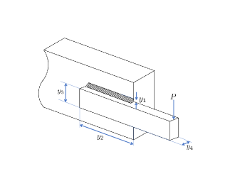
Figure 10: Welded beam

$$\small\begin{array}[]{l}min\;F(y_{1},y_{2},y_{3},y_{4})=1.10471y_{1}^{2}+0.04811y_{3}y_{4}(14.0+y_{2})\\ \mbox{Subject to:}\\ g1(\mathbf{y})=\tau(\mathbf{y})-\tau_{max}\leq 0\\ g2(\mathbf{y})=\sigma(\mathbf{y})-\sigma_{max}\leq 0\\ g3(\mathbf{y})=\delta(\mathbf{y})-\delta_{max}\leq 0\\ g4(\mathbf{y})=y_{1}-y_{4}\leq 0\\ g5(\mathbf{y})=P-\gamma(\mathbf{y})\leq 0\\ g6(\mathbf{y})=0.125-y_{1}\leq 0\\ g7(\mathbf{y})=0.10471y_{1}^{2}+0.04811y_{3}y_{4}(14.0+y_{2})-5.0\leq 0\\ \mbox{where:}\\ P=6000\;lb,\;L=14\;in,\;\sigma_{max}=30000\;psi,\\ \delta_{max}=0.25\;in,\;E=30e6\;psi,\;G=12e6\;psi\\ M=P(L+\frac{y_{2}}{2}),\;R=\sqrt{\frac{y_{2}^{2}}{4}+\left(\frac{y_{1}+y_{3}}{2}\right)^{2}}\\ J=2\left(\sqrt{2}y_{1}y_{2}\left(\frac{y_{2}^{2}}{12}+\left(\frac{y_{1}+y_{3}}{2}\right)^{2}\right)\right)\\ \tau^{\prime}=\frac{P}{\sqrt{2}y_{1}y_{2}},\;\tau^{\prime\prime}=\frac{MR}{J}\\ \tau(\mathbf{y})=\sqrt{(\tau^{\prime})^{2}+2\tau^{\prime}\tau^{\prime\prime}\frac{y_{2}}{2R}+(\tau^{\prime\prime})^{2}},\;\sigma(\mathbf{y})=\frac{6PL}{y_{3}^{2}y_{4}}\\ \delta(\mathbf{y})=\frac{4PL^{3}}{Ey_{3}^{3}y_{4}},\;\gamma(\mathbf{y})=\frac{4.013E\sqrt{\frac{y_{3}^{2}y_{4}^{6}}{36}}}{L^{2}}\left(1-\frac{y_{3}}{2L}\sqrt{\frac{E}{4G}}\right)\\ \end{array}$$ (3)

where $0.1\leq y_{1}\leq 2$, $0.1\leq y_{2}\leq 10$, $0.1\leq y_{3}\leq 10$ y $0.1\leq y_{4}\leq 2$. For this model, the result obtained by the CCAA is compared with the results published in (Chen et al., 2020) and (Coello, 2000), which take into consideration $8$ different meta-heuristic algorithms. Again, $50$ independent runs of the CCAA were made and the best result was taken. In each run, $5$ $smart\_cells$ and $4$ neighbors were used for each $smart\_cell$, in addition to $2000$ evaluations of $F$ in order to make the experiment comparable to the references consulted. The best design obtained by the CCAA are shown in Table 14. It can be seen that the CCAA calculated the second-best design at the cost of $1.7248$. Therefore, the CCAA is competitive in the optimization of the WBD problem.

Table 14: Comparison of meta-heuristics for the WBD problem.

Algorithm	$y_{1}$	$y_{2}$	$y_{3}$	$y_{4}$	$F_{min}$
RDWOA	$0.205618$	$3.252958$	$9.04447$	$0.20569$	$1.6961$
CCAA	$0.20573$	$3.4705$	$9.03662$	$0.20573$	$1.7248$
IHS	$0.20573$	$3.47049$	$9.03662$	$0.20573$	$1.7248$
RO	$0.203687$	$3.528467$	$9.004233$	$0.207241$	$1.735344$
GA-Coello	$0.2088$	$3.4205$	$8.9975$	$0.2100$	$1.7483$
HS	$0.2442$	$6.2231$	$8.2915$	$0.2433$	$2.3807$
David	$0.2434$	$6.2552$	$8.2915$	$0.2444$	$2.3841$
Simple	$0.2792$	$5.6256$	$7.7512$	$0.2796$	$2.5307$
Random	$0.4575$	$4.7313$	$5.0853$	$0.6600$	$4.1185$

4.4.4 Cantilever beam design (CBD)

The cantilever beam design problem (CBD) objective is to obtain the minimum weight of a rigid structural element supported only on one side by another vertical element (Mirjalili, 2015). The model consists of five hollow elements that have a square section. There is a vertical load in the last part of the structure, and there is a vertical displacement restriction. The system to be designed can be seen in Fig. 11.

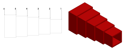
Figure 11: Cantilever beam.

The problem is formulated in Eq. 4.

$$\small\begin{array}[]{l}min\;F(y_{1},y_{2},y_{3},y_{4},y_{5})=0.6224(y_{1}+y_{2}+y_{3}+y_{4}+y_{5})\\ \mbox{Subject to:}\\ g(y_{1},y_{2},y_{3},y_{4},y_{5})=\frac{61}{y_{1}^{3}}+\frac{37}{y_{2}^{3}}+\frac{19}{y_{3}^{3}}+\frac{7}{y_{4}^{3}}+\frac{1}{y_{5}^{3}}\leq 1\\ \end{array}$$ (4)

where $0.01\leq y_{1},y_{2},y_{3},y_{4},y_{5}\leq 100$. For this model, the result obtained by the CCAA is compared with the results published in (Wu et al., 2020) and (Mirjalili, 2015) taking $7$ different meta-heuristic algorithms. Again, $50$ independent runs of the CCAA were made and the best result was taken. In each run, $5$ $smart\_cells$ and $4$ neighbors were used for each $smart\_cell$, with a maximum of $12000$ evaluations of $F$ to have an experiment similar to the one reported in (Mirjalili, 2015).

Table 15: Comparison of meta-heuristics for the CBD problem.

Algorithm	$y_{1}$	$y_{2}$	$y_{3}$	$y_{4}$	$y_{5}$	$F_{min}$
ALO	$6.01812$	$5.31142$	$4.48836$	$3.49751$	$2.158329$	$1.33995$
CCAA	$6.01698$	$5.30917$	$4.49428$	$3.50147$	$2.15266$	$1.33996$
SOS	$6.01878$	$5.30344$	$4.49587$	$3.49896$	$2.15564$	$1.33996$
CS	$6.0089$	$5.3049$	$4.5023$	$3.5077$	$2.1504$	$1.33999$
MMA	$6.0100$	$5.3000$	$4.4900$	$3.4900$	$2.1500$	$1.3400$
GCA_I	$6.0100$	$5.30400$	$4.4900$	$3.4980$	$2.1500$	$1.3400$
GCA_II	$6.0100$	$5.3000$	$4.4900$	$3.4900$	$2.1500$	$1.3400$

The reference values and the best design achieved by the CCAA are shown in Table 15. It can be seen that the CCAA had the second-best design with a cost of $1.33996$. Therefore, the CCAA is also well-suited to optimize this engineering problem.

5 IIR Filter Design Optimization

IIR filters are one of the main types of filters applied in digital signal processing to separate overlapping signals and restore signals that have been distorted (Harris, 2004). This section reports the design of adaptive IIR filters using the CCAA algorithm and comparing the results with other specialized algorithms recently published.

The design of infinite impulse response (IIR) filters has become a recurring research topic since they are more efficient than other types of filters. The IIR filter design problem has been addressed using meta-heuristic algorithms, determining the parameters to obtain an optimal model of the unknown plant, minimizing the error’s cost function. The IIR filter transfer function is defined by:

$$\frac{Y(z)}{U(z)}=\frac{b_{0}+b_{1}z^{-1}+b_{2}z^{-2}+\ldots+b_{n}z^{-n}}{1+a_{1}z^{-1}+a_{2}z^{-2}+\ldots+a_{m}z^{-m}}$$ (5)

where $Y(z)$ and $U(z)$ are the output and input respectively, $[a_{1},a_{2},\ldots a_{n}]$ and $[b_{0},b_{1},$ $\ldots,b_{n}]$ are the real coefficients of the numerator and denominator, $n$ and $m$ are the maximum degree of the polynomials of the numerator and denominator respectively.

According to Fig. 12, the problem of the adaptive IIR filter is to identify the unknown model whose transfer function is described by Eq. 5, $d(k)$ is the output of the unknown system, and a noise component $v(k)$ is added to generate the output $y(k)$. The adaptive IIR filter block receives the same input as the unknown IIR system block $u(k)$. It also receives as input the coefficients of the numerator and denominator generated by the meta-heuristic algorithm $\Theta(k)=[a_{1},a_{2}.\ldots a_{m},b_{0},b_{1},\ldots,b_{n}]$, the output generated is an estimated response $\hat{y}(k)$. The deviation of the estimated signal $\hat{y}(k)$ to the output signal of the unknown system $y(k)$ is known as the mean square error MSE and is represented by $e(k)$. Mathematically, the adaptive IIR filter problem can be modeled as an optimization problem of minimizing the signal $e(k)$, that is:

$$Min\;e(k)=\frac{1}{L}\sum_{k=1}^{L}(y(k)-\hat{y}(k))^{2}$$ (6)

where $L$ is the length of the vector or input signal $u(k)$.

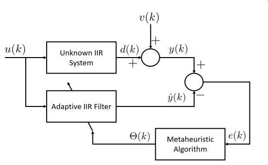
Figure 12: Parameter identification scheme in adaptive IIR filters.

The $10$ cases analyzed in this work are IIR filter models reviewed in the references (Krusienski and Jenkins, 2005), (Panda et al., 2011), (Jiang et al., 2015), (Lagos-Eulogio et al., 2017) and (Zhao et al., 2019). Table 16 shows the models for examples I, II, III, IV, V, VI, VII, VIII, IX, and X. The identification of parameters is carried out through a transfer function of full order.

Table 16: Ten IIR system identification problems

Problems	The transfer function	The transfer function of the
	of IIR plant $H_{p}(z)$	adaptive IIR filter model $H_{a}(z)$
Example I	$\frac{0.05-0.4z^{-1}}{1-1.1314z^{-1}+0.25z^{-2}}$	$\frac{b_{0}-b_{1}z^{-1}}{1-a_{1}z^{-1}-a_{2}z^{-2}}$
Example II	$\frac{-0.2-0.4z^{-1}+0.5z^{-2}}{1-0.6z^{-1}+0.25z^{-2}-0.2z^{-3}}$	$\frac{b_{0}+b_{1}z^{-1}+b_{2}z^{-2}}{1-a_{1}z^{-1}-a_{2}z^{-2}-a_{3}z^{-3}}$
Example III	$\frac{1-0.9z^{-1}+0.81z^{-2}-0.729z^{-3}}{1+0.04z^{-1}+0.2775z^{-2}-0.2101z^{-3}+0.14z^{-4}}$	$\frac{b_{0}+b_{1}z^{-1}+b_{2}z^{-2}+b_{3}z^{-3}}{1-a_{1}z^{-1}-a_{2}z^{-2}-a_{3}z^{-3}-a_{4}z^{-4}}$
Example IV	$\frac{0.1084+0.5419z^{-1}+1.0837z^{-2}+1.0837z^{-3}+0.5419z^{-4}+0.1084z^{-5}}{1+0.9853z^{-1}+0.9738z^{-2}-0.3854z^{-3}+0.1112z^{-4}+0.0113z^{-5}}$	$\frac{b_{0}+b_{1}z^{-1}+b_{2}z^{-2}+b_{3}z^{-3}+b_{4}z^{-4}+b_{5}z^{-5}}{1-a_{1}z^{-1}-a_{2}z^{-2}-a_{3}z^{-3}-a_{4}z^{-4}-a_{5}z^{-5}}$
Example V	$\frac{1-0.4z^{-2}-0.65z^{-4}+0.26z^{-6}}{1-0.77z^{-2}-0.8498z^{-4}+0.6486z^{-6}}$	$\frac{b_{0}+b_{2}z^{-2}+b_{4}z^{-4}+b_{6}z^{-6}}{1-a_{2}z^{-2}-a_{4}z^{-4}-a_{6}z^{-6}}$
Example VI	$\frac{1}{1-1.4z^{-1}+0.49z^{-2}}$	$\frac{b_{0}}{1-a_{1}z^{-1}-a_{2}z^{-2}}$
Example VII	$\frac{1}{1-1.2z^{-1}+0.6z^{-2}}$	$\frac{b_{0}}{1-a_{1}z^{-1}-a_{2}z^{-2}}$
Example VIII	$\frac{1.25z^{-1}-0.25z^{-2}}{1-0.3z^{-1}+0.4z^{-2}}$	$\frac{b_{1}z^{-1}+b_{2}z^{-2}}{1-a_{1}z^{-1}-a_{2}z^{-2}}$
Example IX	$\frac{1}{(1-0.5z^{-1})^{3}}$	$\frac{b_{0}}{1-a_{1}z^{-1}-a_{2}z^{-2}-a_{3}z^{-3}}$
Example X	$\frac{-0.3+0.4z^{-1}-0.5z^{-2}}{1-1.2z^{-1}+0.5z^{-2}-0.1z^{-3}}$	$\frac{b_{0}+b_{1}z^{-1}+b_{2}z^{-2}}{1-a_{1}z^{-1}-a_{2}z^{-2}-a_{3}z^{-3}}$

It is necessary to mention that the adaptive IIR filter design problem requires robust algorithms since the systems are non-linear, non-differentiable, and multimodal. Recent hybrid algorithms have been proposed for this problem. For example, in (Jiang et al., 2015), a hybrid algorithm is implemented with a PSO (particle swarm optimization) and a gravitational algorithm (GSA), which is called HPSO-GSA. This algorithm generates a co-evolutionary technique, taking advantage of the PSO’s ability to share information between particles and the memory of the best position obtained, and the GSA’s force and mass acceleration to determine the best search direction. Similarly, in (Lagos-Eulogio et al., 2017) the parameter estimation problem is addressed using a hybrid algorithm, in this case, a combination of concepts of a cellular-automata neighborhood, PSO, and the Differential Evolution algorithm (CPSO-DE). In this way, CPSO-DE is able to modify the trajectory of the particles to leave the local optimum, while the PSO and the DE focus on finding a higher quality solution. The performance of the CCAA algorithm is compared with two algorithms that also use cellular automata concepts (CPSO and CPSO-DE), with a gravitational hybrid algorithm (HPSO-GSA), and with two recent algorithms (GWO and MSCA). To make a more fair comparison, a population of $100$ individuals was applied for the HPSO-GSA, GWO, and MSCA. For the CPSO, CPSO-DE and CCAA, $20$ $smart\_cells$ and $5$ neighbors for $smart\_cell$ were utilized. Besides, $50$ runs were carried out for every algorithm, each applying a total number of $500$ iterations.

Table 17 shows the MSE statistical results for the best, worst, average, mean, and standard deviation for each example for the first $5$ IIR filters. For the cases I and II, the CCAA and CPSO-DE algorithms identified the parameters with an MSE of $0$, obtaining the best of the $50$ runs. For the case III to V, the CPSO-DE algorithm obtained a higher performance than the others for calculating the best parameter estimation. In these cases, the CCAA obtained positions $3$, $3$ and $2$ respectively in the best value, and positions $3$, $2$ and $2$ in the best average value. The best parameter estimations for these $5$ filters are presented in Tables 18 - 22.

Table 17: Experimental results (MSE) of algorithms for Test Examples I,II, III, IV, V

Problems	Measure	Mean square error (MSE)
		HPSO-GSA	CPSO-DE	CPSO	GWO	MSCA	CCAA
Example I	Best	2.305e-22	0	1.249e-23	1.237e-07	1.914e-05	0
	Worst	1.006e-20	0	2.504e-01	1.192e-02	1.124e-01	0
	Average	3.384e-21	0	9.334e-03	2.389e-03	3.184e-03	0
	Median	2.524e-21	0	2.734e-18	3.807e-06	2.867e-04	0
	SD	2.348e-21	0	4.632e-02	4.215e-03	1.592e-02	0
Example II	Best	1.118e-21	0	1.914e-32	5.788e-08	2.865e-04	0
	Worst	5.902e-03	1.222e-32	6.121e-03	4.858e-03	3.943e-02	5.589e-03
	Average	1.453e-03	6.079e-34	1.424e-03	1.210e-03	6.084e-03	1.123e-04
	Median	4.134e-21	0	4.572e-04	2.451e-07	4.250e-03	0
	SD	2.092e-03	2.221e-33	1.865e-03	1.643e-03	7.301e-03	7.904e-04
Example III	Best	9.300e-21	0	8.728e-12	1.242e-05	1.648e-03	1.528e-14
	Worst	2.594e-02	1.082e-31	2.794e+00	1.026e-01	3.384e-01	4.980e-02
	Average	3.288e-03	8.660e-33	1.270e-01	1.173e-02	5.761e-02	3.321e-03
	Median	1.566e-13	0	1.206e-03	1.357e-03	2.416e-02	5.887e-05
	SD	7.083e-03	1.852e-32	4.351e-01	2.357e-02	6.200e-02	9.963e-03
Example IV	Best	3.124e-06	1.768e-08	8.645e-06	1.139e-05	1.277e-03	1.316e-05
	Worst	3.054e-01	5.904e-06	2.456e+00	8.225e-03	5.007e-02	4.019e-03
	Average	8.206e-03	2.540e-06	2.037e-01	1.449e-03	1.220e-02	6.618e-04
	Median	3.056e-04	2.715e-06	1.151e-03	9.029e-04	1.091e-02	2.033e-04
	SD	4.308e-02	1.280e-06	5.263e-01	1.760e-03	9.180e-03	9.653e-04
Example V	Best	5.336e-04	2.964e-31	5.072e-04	7.645e-04	1.811e-03	2.416e-05
	Worst	3.620e-02	3.139e-09	2.673e-01	3.050e-02	1.015e-01	1.191e-02
	Average	8.303e-03	6.453e-11	1.790e-02	9.688e-03	1.746e-02	2.697e-03
	Median	9.395e-03	2.014e-18	8.639e-03	9.184e-03	1.518e-02	8.339e-04
	SD	6.501e-03	4.437e-10	4.837e-02	5.463e-03	1.471e-02	3.745e-03

Table 18: The parameter estimation of algorithms for Example I

Parameters	Actual values	Parameter estimation value
		HPSO-GSA	CPSO-DE	CPSO	GWO	MSCA	CCAA
$b_{0}$	0.050	0.050	0.050	0.050	0.049	0.043	0.050
$b_{1}$	-0.400	-0.400	-0.400	-0.400	-0.399	-0.393	-0.400
$a_{1}$	1.131	1.131	1.131	1.131	1.132	1.133	1.131
$a_{2}$	-0.250	-0.250	-0.250	-0.250	-0.251	-0.2514	-0.250

Table 19: The parameter estimation of algorithms for Example II

Parameters	Actual values	Parameter estimation value
		HPSO-GSA	CPSO-DE	CPSO	GWO	MSCA	CCAA
$b_{0}$	-0.20	-0.20	-0.20	-0.20	-0.19	-0.19	-0.20
$b_{1}$	-0.40	-0.40	-0.40	-0.40	-0.39	-0.39	-0.40
$b_{2}$	0.50	0.50	0.50	0.50	0.51	0.51	0.50
$a_{1}$	0.60	0.60	0.60	0.60	0.61	0.64	0.60
$a_{2}$	-0.25	-0.25	-0.25	-0.25	-0.24	-0.23	-0.25
$a_{3}$	0.20	0.20	0.20	0.20	0.21	0.21	0.20

Table 20: The parameter estimation of algorithms for Example III

Parameters	Actual values	Parameter estimation value
		HPSO-GSA	CPSO-DE	CPSO	GWO	MSCA	CCAA
$b_{0}$	1.0000	1.0000	1.0000	0.9998	0.9996	1.0250	0.9991
$b_{1}$	-0.9000	-0.9000	-0.9000	-0.9042	-0.8928	-0.9313	-0.8975
$b_{2}$	0.8100	0.8100	0.8100	0.8093	0.8071	0.7354	0.8154
$b_{3}$	-0.7290	-0.7290	-0.7290	-0.7309	-0.7283	-0.7019	-0.7261
$a_{1}$	-0.0400	-0.0400	-0.0400	-0.0362	-0.0463	-0.0031	-0.0424
$a_{2}$	-0.2775	-0.2775	-0.2775	-0.2733	-0.2795	-0.1994	-0.2855
$a_{3}$	0.2101	0.2101	0.2101	0.2131	0.2110	0.2579	0.2018
$a_{4}$	-0.1400	-0.1400	-0.1400	-0.1395	-0.1363	-0.1390	-0.1442

Table 21: The parameter estimation of algorithms for Example IV

Parameters	Actual values	Parameter estimation value
		HPSO-GSA	CPSO-DE	CPSO	GWO	MSCA	CCAA
$b_{0}$	0.1084	0.1083	0.1084	0.1083	0.1106	0.1040	0.1078
$b_{1}$	0.5419	0.4900	0.4609	0.4536	0.4676	0.4798	0.4332
$b_{2}$	1.0840	0.8416	0.7088	0.6748	0.7262	0.7193	0.6129
$b_{3}$	1.0840	0.6541	0.4176	0.3589	0.3822	0.4713	0.3065
$b_{4}$	0.5419	0.1908	-0.0023	-0.0484	-0.1161	0.03742	-0.0184
$b_{5}$	0.1084	-0.0038	-0.0675	-0.0821	-0.1463	-0.0045	-0.0189
$a_{1}$	-0.9853	-0.5027	-0.2384	-0.1682	-0.3329	-0.3064	-0.0012
$a_{2}$	-0.9738	-0.6778	-0.5157	-0.4804	-0.3086	-0.5344	-0.5806
$a_{3}$	-0.3864	-0.0534	0.1316	0.1806	0.1153	-0.0100	0.2203
$a_{4}$	-0.1112	-0.0536	-0.0227	-0.0183	0.0952	-0.0090	-0.0916
$a_{5}$	-0.0113	0.0079	0.0192	0.0236	-0.0006	-0.0013	0.0267

For cases VI, VII, VIII, IX, and X, the CCAA achieves better performance than the other algorithms (Table 23). In all cases, the CCAA achieves an MSE of $0$ for all statistics, as well as the CPSO algorithm achieves it for cases VII and VIII and CPSO-DE for case IX.

Table 22: The parameter estimation of algorithms for Example V

Parameters	Actual values	Parameter estimation value
		HPSO-GSA	CPSO-DE	CPSO	GWO	MSCA	CCAA
$b_{0}$	1.0000	0.9952	1.0000	0.9911	1.0030	0.9290	1.0020
$b_{2}$	-0.4000	0.0951	-0.4016	0.0310	0.8110	0.3474	0.1533
$b_{4}$	-0.6500	-0.4787	-0.6504	-0.4870	-0.2160	-0.2686	-0.4490
$b_{6}$	0.2600	0.0587	0.2606	0.0794	-0.2203	-0.0571	0.0338
$a_{2}$	0.7700	0.2884	0.7716	0.3439	-0.4426	-0.0001	0.2150
$a_{4}$	0.8498	0.8518	0.8497	0.8420	0.8445	0.8281	0.8424
$a_{6}$	-0.6486	-0.2361	-0.6499	-0.2729	0.4056	0.0442	-0.1625

Table 23: Experimental results (MSE) of algorithms for Test Examples VI, VII, VIII, IX, X

Problems	Measure	Mean square error (MSE)
		HPSO-GSA	CPSO-DE	CPSO	GWO	MSCA	CCAA
Example VI	Best	4.779e-22	0	6.777e-27	9.614e-07	5.878e-05	0
	Worst	2.158e-20	0	3.560e+00	2.908e+00	5.688e-01	0
	Average	6.638e-21	0	7.121e-02	8.731e-02	1.494e-02	0
	Median	5.104e-21	0	1.456e-18	6.153e-06	2.239e-03	0
	SD	5.239e-21	0	5.034e-01	4.234e-01	8.003e-02	0
Example VII	Best	6.540e-23	0	0	1.156e-07	6.273e-05	0
	Worst	3.137e-21	2.128e-31	0	5.108e-06	3.023e-03	0
	Average	1.157e-21	8.506e-33	0	1.523e-06	7.333e-04	0
	Median	9.449e-22	0	0	1.194e-06	4.279e-04	0
	SD	7.713e-22	4.209e-32	0	1.142e-06	6.875e-04	0
Example VIII	Best	1.626e-22	0	0	3.298e-08	1.997e-05	0
	Worst	2.581e-21	4.578e-33	0	7.673e-03	8.759e-03	0
	Average	8.244e-22	9.156e-35	0	9.694e-04	1.005e-03	0
	Median	6.897e-22	0	0	2.495e-07	1.737e-04	0
	SD	5.130e-22	6.475e-34	0	2.432e-03	2.289e-03	0
Example IX	Best	9.748e-14	0	1.798e-05	2.513e-05	7.443e-04	0
	Worst	8.902e-02	0	2.059e-01	3.162e+00	1.448e-01	0
	Average	6.291e-03	0	4.343e-02	1.076e-01	4.313e-02	0
	Median	6.838e-04	0	3.058e-02	2.315e-02	2.312e-02	0
	SD	1.461e-02	0	4.427e-02	4.426e-01	4.259e-02	0
Example X	Best	1.772e-21	0	2.172e-16	9.734e-07	2.365e-04	0
	Worst	9.592e-02	2.640e-32	8.775e-02	8.765e-02	9.275e-02	0
	Average	5.284e-03	2.833e-33	7.671e-03	1.015e-02	1.519e-02	0
	Median	1.582e-17	0	1.450e-09	2.376e-03	5.322e-03	0
	SD	2.116e-02	7.816e-33	2.154e-02	1.775e-02	2.393e-02	0

The best parameter estimations for the last $5$ filters are presented in Tables 24 - 28, and the convergence curves in the parameter estimation of the $10$ cases are presented in Fig. 13.

Table 24: The parameter estimation of algorithms for Example VI

Parameters	Actual values	Parameter estimation value
		HPSO-GSA	CPSO-DE	CPSO	GWO	MSCA	CCAA
$b_{0}$	1.00	1.00	1.00	1.00	1.01	1.01	1.00
$a_{1}$	1.40	1.40	1.40	1.40	1.40	1.39	1.40
$a_{2}$	-0.49	-0.49	-0.49	-0.49	-0.48	-0.48	-0.49

Table 25: The parameter estimation of algorithms for Example VII

Parameters	Actual values	Parameter estimation value
		HPSO-GSA	CPSO-DE	CPSO	GWO	MSCA	CCAA
$b_{0}$	1.00	1.00	1.00	1.00	0.99	0.99	1.00
$a_{1}$	1.20	1.20	1.20	1.20	1.20	1.201	1.20
$a_{2}$	-0.60	-0.60	-0.60	-0.60	-0.60	-0.61	-0.60

Table 26: The parameter estimation of algorithms for Example VIII

Parameters	Actual values	Parameter estimation value
		HPSO-GSA	CPSO-DE	CPSO	GWO	MSCA	CCAA
$b_{1}$	1.25	1.25	1.25	1.25	1.25	1.24	1.25
$b_{2}$	-0.25	-0.25	-0.25	-0.25	-0.25	-0.24	-0.25
$a_{1}$	0.30	0.30	0.30	0.30	0.30	0.29	0.30
$a_{2}$	-0.40	-0.40	-0.40	-0.40	-0.40	-0.40	-0.40

Table 27: The parameter estimation of algorithms for Example IX

Parameters	Actual values	Parameter estimation value
		HPSO-GSA	CPSO-DE	CPSO	GWO	MSCA	CCAA
$b_{0}$	1.000	0.999	1.000	0.999	0.995	0.969	1.000
$a_{1}$	1.500	1.500	1.500	1.501	1.507	1.524	1.500
$a_{2}$	-0.750	-0.750	-0.750	-0.751	-0.761	-0.786	-0.750
$a_{3}$	0.125	0.125	0.125	0.125	0.130	0.140	0.125

Table 28: The parameter estimation of algorithms for Example X

Parameters	Actual values	Parameter estimation value
		HPSO-GSA	CPSO-DE	CPSO	GWO	MSCA	CCAA
$b_{0}$	-0.300	-0.300	-0.300	-0.300	-0.300	-0.328	-0.300
$b_{1}$	0.400	0.400	0.400	0.400	0.400	0.422	0.400
$b_{2}$	-0.500	-0.500	-0.500	-0.500	-0.500	-0.522	-0.500
$a_{1}$	1.200	1.200	1.200	1.200	1.194	1.169	1.200
$a_{2}$	-0.500	-0.500	-0.500	-0.500	-0.487	-0.471	-0.500
$a_{3}$	0.100	0.100	0.100	0.100	0.093	0.096	0.100

Figure 13: Convergence of the MSE curve for the IIR filters

(a) Example I

(b) Example II

(c) Example III

(d) Example IV

(e) Example V

(f) Example VI

(g) Example VII

(h) Example VIII

(i) Example IX

(j) Example X

In summary, for cases I, II, and VI to X, the CCAA algorithm achieved a complete parameter identification, and for cases I and VI to X, the CCAA obtained an MSE of $0$ in all the statistics. In general, for the 10 cases, the CCAA, CPSO-DE and CPSO were the only algorithms with a complete parameter identification, the CPSO-DE in $8$ cases and the CCAA in $7$ cases. The CCAA had $6$ best average values, and the CPSO-DE had $7$ best average values, resulting the best algorithms overall. These results demonstrate that the CCAA can be very useful for the design of adaptive IIR filters, and that the meta-heuristics applying cellular automata concepts can be extremely helpful to optimize challenging problems. Note that the source codes of the CCAA algorithm can be downloaded from https://github.com/juanseck/CCAA.git.

6 Conclusions and future work

This study presented a new global optimization algorithm called CCAA, which uses a neighborhood and evolution rules inspired by cellular automata concepts, such as local interactions between solutions and different evolution rules. These elements allow the exploration and exploitation operations to be carried out concurrently and randomly for each $smart\_cell$ in the solution population.

This strategy allows the CCAA to establish a proper balance of local and global changes and information exchange between $smart\_cells$ during the search for the optimal solution. The experimental validation was carried out with $33$ test functions that were widely used in recent literature to analyze the exploration, exploitation, escape of local optima, and the convergence behavior of the proposed algorithm, analyzing the performance of the CCAA for problems on 30, 500, and fixed dimensions. The experimental results obtained were compared with several recent meta-heuristic algorithms recognized for their excellent performance. The comparison showed that the CCAA is competitive enough to calculate an optimal solution for most problems.

To verify the performance of the CCAA, $5$ engineering design problems (GTD, PVD, WBD, CBD, and IIR filter design) were also addressed. The results also demonstrated the effectiveness of the CCAA to find quality solutions in these types of problems, showing that the CCAA is very competitive with respect to recently published meta-heuristic optimizers.

In future applications, it is intended to apply improvements of the CCAA for other engineering problems, such as the design of reduced-order IIR filters. This article proposed the application of the CCAA to solve single-objective optimization problems. However, many problems involve multiple objectives for real situations. In this sense, a proposal for future work is to use the CCCAA to optimize continuous and discrete multi-objective problems, such as task scheduling problems, route scheduling, aeronautical modeling problems, classification problems, power dispatch problems, among others. The application of different and diverse evolution rules is also proposed to improve the performance of the CCAA.

References

- Atul Kumar Dwivedi and Londhe (2018) Atul Kumar Dwivedi, S.G., Londhe, N.D., 2018. Review and analysis of evolutionary optimization-based techniques for fir filter design. Circuits Syst Signal Process 37, 4409–4430.
- Chatterjee et al. (2020) Chatterjee, A., Kim, E., Reza, H., 2020. Adaptive dynamic probabilistic elitist ant colony optimization in traveling salesman problem. SN Computer Science 1, 1–8.
- Chen et al. (2020) Chen, H., Yang, C., Heidari, A.A., Zhao, X., 2020. An efficient double adaptive random spare reinforced whale optimization algorithm. Expert Systems with Applications 154, 113018.
- Coello (2000) Coello, C.A.C., 2000. Use of a self-adaptive penalty approach for engineering optimization problems. Computers in Industry 41, 113–127.
- Dorigo and Gambardella (1997) Dorigo, M., Gambardella, L.M., 1997. Ant colony system: a cooperative learning approach to the traveling salesman problem. IEEE Transactions on evolutionary computation 1, 53–66.
- Eberhart and Kennedy (1995) Eberhart, R., Kennedy, J., 1995. A new optimizer using particle swarm theory, in: MHS’95. Proceedings of the Sixth International Symposium on Micro Machine and Human Science, Ieee. pp. 39–43.
- Gandomi et al. (2013) Gandomi, A.H., Yang, X.S., Alavi, A.H., 2013. Cuckoo search algorithm: a metaheuristic approach to solve structural optimization problems. Engineering with computers 29, 17–35.
- Gupta et al. (2020) Gupta, S., Deep, K., Mirjalili, S., Kim, J.H., 2020. A modified sine cosine algorithm with novel transition parameter and mutation operator for global optimization. Expert Systems with Applications , 113395.
- Harris (2004) Harris, F.J., 2004. Multirate signal processing for communication systems. Prentice Hall PTR.
- Hernández-Gress et al. (2020) Hernández-Gress, E.S., Seck-Tuoh-Mora, J.C., Hernández-Romero, N., Medina-Marín, J., Lagos-Eulogio, P., Ortíz-Perea, J., 2020. The solution of the concurrent layout scheduling problem in the job-shop environment through a local neighborhood search algorithm. Expert Systems with Applications 144, 113096.
- Holland (1984) Holland, J.H., 1984. Genetic algorithms and adaptation, in: Adaptive Control of Ill-Defined Systems. Springer, pp. 317–333.
- Huang et al. (2019) Huang, H., Zhu, M., Wang, J., 2019. An improved artificial bee colony algorithm based on special division and intellective search. JIPS 15, 433–439.
- Jiang et al. (2015) Jiang, S., Wang, Y., Ji, Z., 2015. A new design method for adaptive iir system identification using hybrid particle swarm optimization and gravitational search algorithm. Nonlinear Dynamics 79, 2553–2576.
- Karaboga (2005) Karaboga, D., 2005. An idea based on honey bee swarm for numerical optimization. Technical Report. Technical report-tr06, Erciyes university, engineering faculty, computer engineering department.
- Krusienski and Jenkins (2005) Krusienski, D.J., Jenkins, W.K., 2005. Design and performance of adaptive systems based on structured stochastic optimization strategies. IEEE circuits and systems magazine 5, 8–20.
- Kumar and Davim (2020) Kumar, K., Davim, J.P., 2020. Optimization Using Evolutionary Algorithms and Metaheuristics: Applications in Engineering. 1 ed., CRC Press.
- Lagos-Eulogio et al. (2017) Lagos-Eulogio, P., Seck-Tuoh-Mora, J., Hernandez-Romero, N., Medina-Marin, J., 2017. A new design method for adaptive iir system identification using hybrid cpso and de. Nonlinear Dynamics 88, 2371–2389.
- Liu et al. (2020) Liu, Y., Cao, B., Li, H., 2020. Improving ant colony optimization algorithm with epsilon greedy and levy flight. Complex Intell. Syst. 24, 54.
- McIntosh (2009) McIntosh, H.V., 2009. One dimensional cellular automata. Luniver Press.
- de Melo and Banzhaf (2018) de Melo, V.V., Banzhaf, W., 2018. Drone squadron optimization: a novel self-adaptive algorithm for global numerical optimization. Neural Computing and Applications 30, 3117–3144.
- Mirjalili (2015) Mirjalili, S., 2015. The ant lion optimizer. Advances in engineering software 83, 80–98.
- Mirjalili and Lewis (2016) Mirjalili, S., Lewis, A., 2016. The whale optimization algorithm. Advances in engineering software 95, 51–67.
- Mirjalili et al. (2014) Mirjalili, S., Mirjalili, S.M., Lewis, A., 2014. Grey wolf optimizer. Advances in engineering software 69, 46–61.
- Moayedi et al. (2020) Moayedi, H., Gör, M., Khari, M., Foong, L.K., Bahiraei, M., Bui, D.T., 2020. Hybridizing four wise neural-metaheuristic paradigms in predicting soil shear strength. Measurement 156, 107576.
- Mukhtar et al. (2019) Mukhtar, A., Tayal, V.K., Singh, H., 2019. Pso optimized pid controller design for the process liquid level control, in: 2019 3rd International Conference on Recent Developments in Control, Automation Power Engineering (RDCAPE), pp. 590–593.
- Panda et al. (2011) Panda, G., Pradhan, P.M., Majhi, B., 2011. Iir system identification using cat swarm optimization. Expert Systems with Applications 38, 12671–12683.
- Qiao et al. (2020) Qiao, W., Moayedi, H., Foong, L.K., 2020. Nature-inspired hybrid techniques of iwo, da, es, ga, and ica, validated through a k-fold validation process predicting monthly natural gas consumption. Energy and Buildings , 110023.
- Qu et al. (2020) Qu, C., Gai, W., Zhang, J., Zhong, M., 2020. A novel hybrid grey wolf optimizer algorithm for unmanned aerial vehicle (uav) path planning. Knowledge-Based Systems , 105530.
- Salih et al. (2019) Salih, S.Q., Alsewari, A.A., Yaseen, Z.M., 2019. Pressure vessel design simulation: Implementing of multi-swarm particle swarm optimization, in: Proceedings of the 2019 8th International Conference on Software and Computer Applications, Association for Computing Machinery, New York, NY, USA. p. 120–124.
- Sandgren (1990) Sandgren, E., 1990. Nonlinear integer and discrete programming in mechanical design optimization. Journal of Mechanical Design 112, 223––229.
- Shi et al. (2011) Shi, Y., Liu, H., Gao, L., Zhang, G., 2011. Cellular particle swarm optimization. Information Sciences 181, 4460–4493.
- Tansel Dokeroglua and Cosarb (2019) Tansel Dokeroglua, Ender Sevincb, T.K., Cosarb, A., 2019. A survey on new generation metaheuristic algorithms. Computers & Industrial Engineering 137, 4409––4430.
- Van Den Bergh and Engelbrecht (2006) Van Den Bergh, F., Engelbrecht, A.P., 2006. A study of particle swarm optimization particle trajectories. Information sciences 176, 937–971.
- Wang et al. (2020) Wang, H., Wang, W., Zhou, X., Zhao, J., Wang, Y., Xiao, S., Xu, M., 2020. Artificial bee colony algorithm based on knowledge fusion. Complex & Intelligent Systems , 1–14.
- Wolfram (2002) Wolfram, S., 2002. A new kind of science. volume 5. Wolfram media Champaign, IL.
- Wolpert and Macready (1997) Wolpert, D.H., Macready, W.G., 1997. No free lunch theorems for optimization. IEEE transactions on evolutionary computation 1, 67–82.
- Wu et al. (2020) Wu, J., Wang, Y.G., Burrage, K., Tian, Y.C., Lawson, B., Ding, Z., 2020. An improved firefly algorithm for global continuous optimization problems. Expert Systems with Applications , 113340.
- Yang et al. (2020) Yang, H., Li, Y., Yang, L., Wu, Q., 2020. An improved particle swarm optimization algorithm based on entropy and fitness of particles, in: 2020 12th International Conference on Measuring Technology and Mechatronics Automation (ICMTMA), IEEE. pp. 492–496.
- Yu et al. (2020) Yu, J., Li, R., Feng, Z., Zhao, A., Yu, Z., Ye, Z., Wang, J., 2020. A novel parallel ant colony optimization algorithm for warehouse path planning. Journal of Control Science and Engineering , 5287189.
- Zervoudakis and Tsafarakis (2020) Zervoudakis, K., Tsafarakis, S., 2020. A mayfly optimization algorithm. Computers & Industrial Engineering , 106559.
- Zhao et al. (2019) Zhao, R., Wang, Y., Liu, C., Hu, P., Jelodar, H., Yuan, C., Li, Y., Masood, I., Rabbani, M., Li, H., et al., 2019. Selfish herd optimization algorithm based on chaotic strategy for adaptive iir system identification problem. Soft Computing , 1–48.
- Zhong and Cheng (2020) Zhong, X., Cheng, P., 2020. An improved differential evolution algorithm based on dual-strategy. Mathematical Problems in Engineering , 9767282.