Evaporation of four-dimensional dynamical black holes sourced by the quantum trace anomaly

Paolo Meda^1,3,a, Nicola Pinamonti^2,3,b, Simone Roncallo^1,3,c, Nino Zanghì^1,3,d

¹ Dipartimento di Fisica, Università di Genova, Italy.

² Dipartimento di Matematica, Università di Genova, Italy.

³ Istituto Nazionale di Fisica Nucleare - Sezione di Genova, Italy.

E-mail: ^apaolo.meda@ge.infn.it, ^bpinamont@dima.unige.it ^csimoneroncallo1996@gmail.com,
^dnino.zanghi@ge.infn.it,

Abstract. We study the evaporation of a four-dimensional spherically symmetric black hole formed in a gravitational collapse. We analyze the back-reaction of a massless quantum scalar field conformally coupled to the scalar curvature by means of the semiclassical Einstein equations. We show that the evaporation is linked to an ingoing negative energy flux at the dynamical horizon and that this flux is induced by the quantum matter trace anomaly outside the black hole horizon whenever a suitable averaged energy condition is satisfied. For illustrative purposes, we evaluate the negative ingoing flux and the corresponding rate of evaporation in the case of a null radiating star described by the Vaidya spacetime.

1 Introduction

In semiclassical approximation of quantum gravity, matter is described by quantum fields propagating on a curved classical background in such a way that, given a state $\omega$ of the quantum field, the back-reaction on the classical background is determined by the semiclassical Einstein equations

$$G_{\mu\nu}=8\pi\expectationvalue{{:}T_{\mu\nu}{:}}_{\omega}$$ (1)

in units convention $G=c=\hbar=1$. Here $G_{\mu\nu}$ is the usual Einstein tensor and $\expectationvalue{{:}T_{\mu\nu}{:}}_{\omega}$ is the mean expectation value of the quantum stress-energy tensor in the state $\omega$. The classical background is assumed to be a four-dimensional globally hyperbolic spacetime $(\mathcal{M},g)$, with $\mathcal{M}$ a smooth manifold and $g$ a Lorentzian metric with signature $(-,+,+,+)$. We consider self-consistent solutions in semiclassical gravity. A self-consistent solution is a pair composed by a spacetime metric and a quantum state satisfying eq. (1) at all orders in $\hbar$. Given any such solution, the quantum stress-energy evaluated in $\omega$ gives the Einstein tensor of the spacetime $(\mathcal{M},g)$. Conversely, the Einstein tensor constructed from the metric $g$ yields the expectation value of the quantum stress-energy tensor of the quantum field consistent with $\omega$. It is often argued that solutions of eq. (1) furnish approximations to models of a more fundamental theory of quantum gravity valid in the regime where $R_{\mu\nu\rho\sigma}R^{\mu\nu\rho\sigma}\ll m_{P}^{4}$, with $m_{P}$ denoting the Planck mass, and when the fluctuations of the stress-energy tensor are small [KF93].

In the seminal works [Haw74, Haw75], Hawking showed that a Schwarzschild black hole emits a radiation which can be detected as a flux of particles at large distances from the black hole. This is the well known Hawking radiation, originally obtained assuming no back-reaction and with the quantum matter being in a vacuum state in the asymptotic past. Its power spectrum is thermal with temperature $T_{H}$, the so-called Hawking temperature, given in terms of the black hole mass $M$ by

$$T_{H}=\frac{1}{8\pi k_{B}M}$$ (2)

(in our units convention), with $k_{B}$ being the Boltzmann constant. Under these assumptions, the power of the radiation at future infinity is regarded as describing the evaporation of the black hole. In the adiabatic approximation, the value of the total power emitted is equated to the rate of the loss of mass of the black hole, which turns out to be constant and proportional to $M^{-2}$ (see also [Pag76]).

This standard derivation is defective in various respects. On one hand, the adiabatic approximation is not able to predict the precise form of the horizon of a black hole with non constant mass. Moreover, it misses the dynamical nature of the process of evaporation. It is important to stress that these defects might be cured, at least in principle, within the framework of the semiclassical approximation. Indeed, according to eq. (1), the rate of mass loss turns out to be proportional to a flux of negative energy across the black hole horizon. Though in the absence of the static symmetry the power radiated at infinity is not directly linked to that negative flux of energy at the horizon (and its precise value depends sensibly on the spacetime details), this radiation (if any) can be detected at future infinity. On the contrary, we shall see that the flux of negative energy at the horizon is constrained and forced to be present in the model by the quantum nature of matter in the causal past of the horizon. This is the simple idea we shall exploit to show evaporation.

Preliminarily, we observe that concepts like event horizons and its adiabatic changes are based on global properties of the spacetime. So, in the case of dynamical backgrounds, they need to be replaced by apparent horizons and their evolutions. Indeed, some attempts to study the back-reaction on four-dimensional spherically symmetric black holes have been made, e.g., assuming the geometrical optics approximation, which simplifies the analysis to a two-dimensional problem [Bal84, BB89].

In our work we rely on the semiclassical Einstein equations (1), without making further approximations. Without any appeal to global properties or the explicit form of the stress-energy tensor on the horizon, we shall perform a local analysis of the apparent horizons and show that, in the case of spherically symmetric spacetimes, their dynamics can be constrained by the matter content outside and in the causal past of the black hole. In particular, by considering the stress-energy tensor of a massless, conformally coupled scalar field, and its conservation laws, we shall prove that the evaporation of the black hole is induced by the form of the quantum trace anomaly outside the horizon.

This follows from a very natural condition of the quantum state in the causal past and a mild assumption on the energy outside the horizon, which holds in the case of classical matter. The only quantum property of matter which is used in the argument is the form of the trace anomaly, without which no evaporation can occur. We shall now provide some background and a sketch of our analysis.

Firstly, we recall that the process of evaporation can be semiclassically explained by the presence of an ingoing flux of negative energy on the horizon, violating the classical null energy condition $T(k,k)\geq 0$ for all null vectors $k$ on the horizon. This flux is responsible of the shrink of the dynamical area of the horizon, which can in general increase or decrease respectively during a formation or evaporation process [AK02, AK03, AK04]. Indeed, such a violation on the horizon is not surprising, since it has been proven that a very large class of pointwise energy conditions are not valid when quantum fields are involved, even in flat spacetime (the Casimir effect, for instance).

Secondly, it is well known that in the framework of quantum fields on curved spacetimes, an anomalous term is present in the expectation value of the trace of the quantum stress-energy tensor in any physically reasonable state. Such an anomalous trace is a local contribution which depends only on the geometry and the linear equation of motion of the matter field; it arises in any covariant regularization procedure which gives origin to a covariantly conserved stress-energy tensor ${:}T_{\mu\nu}{:}$, while breaking the classical conformal invariance of $T_{\mu\nu}$ [Wal77, Wal78, BD84, HW04, Mor02]. Moreover, although the expectation value of the quantum stress-energy tensor $\expectationvalue{{:}T_{\mu\nu}{:}}_{\omega}$ is not explicitly available for dynamical black holes (due to the absence of precise control of sufficiently regular states in that context), its trace-anomaly can be evaluated explicitly and independently of the state also for dynamical backgrounds.

Thirdly, black hole evaporation follows from the trace anomaly whenever the stress-energy tensor satisfies a suitable averaged energy condition outside the horizon (see also [E19]). In this extra condition (see below) the pointwise expectation value of a particular component of the stress-energy tensor, is smeared with a suitable strictly positive smooth function supported outside the black hole horizon. Furthermore, this condition needs to hold only for the particular state $\omega$ used in eq. (1) even if it is similar in spirit to other quantum averaged energy conditions, which hold in any quantum state and that have been established in many contexts Finally, we observe that this energy condition can be linked to the geometry described by the semiclassical metric forming with the state $\omega$ a solution of the semiclassical Einstein equations (1). If we also assume that quantum corrections are negligible outside and in the past of the horizon, we get that the energy condition is then satisfied in known models of gravitational collapse like the Oppenheimer-Snyder and Lemaître-Tolman-Bondi models [GP09] and it is also compatible with the collapsing matter described by a classical scalar field in the works of Christodoulou [Chr86a, Chr86b, Chr91].

The paper is organized as follows. In Section 2 we recollect some geometric aspects of spherically symmetric spacetimes and apparent horizons and we recall Hayward’s thermodynamic interpretation of black hole dynamics. In Section 3 we describe the semiclassical process of evaporation due to the negative ingoing flux on the horizon and provide an equation for the variation of the mass. In Section 4 we show that the quantum trace anomaly of a free massless conformally coupled scalar field drives the evaporation assuming a certain averaged quantum energy inequality, which is also satisfied by the background geometry in most realistic classical models of collapse. As an example, we compute the rate of evaporation in the Vaidya spacetime and, as a byproduct, we find that the Schwarzschild spacetime cannot be in equilibrium with the back-reaction of any quantum matter field. Section 5 contains the conclusions and some possible future developments. The technical details to obtain the equation for the variation of the mass and the proof of Theorem 4.1 are collected in the Appendix.

2 Spherically symmetric black holes

A spherically symmetric spacetime $({\mathcal{M}},g)$ is represented by the manifold ${\mathcal{M}}=\Gamma\times\mathds{S}^{2}$, where $\mathds{S}^{2}$ is the two-dimensional sphere of unital radius and $\Gamma$ is a two-dimensional space normal to $\mathds{S}^{2}$, and by the metric

$$\mathrm{d}s^{2}=g_{\mu\nu}\mathrm{d}x^{\mu}\mathrm{d}x^{\nu}=\gamma_{ij}\mathrm{d}x^{i}\mathrm{d}x^{j}+r^{2}\mathrm{d}\theta^{2}+r^{2}\sin^{2}\theta\mathrm{d}\varphi^{2}\ ,\qquad\mu,\nu=0,\dots,3,\quad i,j=1,2,$$

where $r^{2}\in{\mathcal{C}}^{\infty}(\Gamma)$ measures the curvature of each sphere. The two-dimensional spacetime $(\Gamma,\gamma)$ corresponds to the quotient of ${\mathcal{M}}$ with respect to the $SO(3)$ group centered at the origin $r=0$. The invariant $\nabla_{\mu}r\nabla^{\mu}r$ defines the Misner-Sharp energy

$$m\doteq\frac{r}{2}\left(1-\nabla_{\mu}r\nabla^{\mu}r\right),$$ (3)

which describes the energy enclosed inside the sphere of radius $r$ (it is a special case of the Hawking mass for the class of spherically symmetric spacetimes) [MS64, Haw68].

In order to describe an evaporating dynamical black hole, the two-dimensional normal line element $\mathrm{d}\gamma^{2}$ is often represented in the Bardeen-Vaidya metric [Bar81]

$$\mathrm{d}\gamma^{2}=-\mathrm{e}^{2\Psi(v,r)}C(v,r)\mathrm{d}v^{2}+2\mathrm{e}^{\Psi(v,r)}\mathrm{d}v\mathrm{d}r,$$ (4)

where $v$ is the advanced time and

$$C(v,r)\doteq 1-\frac{2m(v,r)}{r}.$$ (5)

In this parametrization, which corresponds to the advanced Eddington-Finkelstein coordinates in the vacuum case, a radial curve at constant $v$ describes an ingoing null geodesic.

Moreover, any two-dimensional metric is locally conformally flat, so we can choose to parametrize $\mathrm{d}\gamma^{2}$ in terms of double-null coordinates $(V,U)$

$$\mathrm{d}\gamma^{2}=-2A(V,U)\mathrm{d}V\mathrm{d}U$$ (6)

with respect to the null normal directions $\partial_{V}$ and $\partial_{U}$. The orientation of the spacetime can be also chosen in such a way that $A(V,U)>0$ and at spatial infinity $\partial_{V}r>0$, $\partial_{U}r<0$. The metric is invariant under any re-parametrization $U\mapsto\tilde{U}(U)$ and $V\mapsto\tilde{V}(V)$, then we can represent the future-directed null normal vector fields as

$$\ell_{+}\doteq A^{-1}\partial_{V},\qquad\ell_{-}\doteq\partial_{U},$$ (7)

which, respectively, describe the outgoing and the ingoing light rays across the spheres that foliates ${\mathcal{M}}$. In this parametrization, the vector field $\ell_{+}$ fulfils the geodesic equation whereas $\ell_{-}$ is an auxiliary vector. The normalization of $\ell_{\pm}$ is such that $g_{\mu\nu}\ell_{+}^{\mu}\ell_{-}^{\nu}=-1$. The local change of coordinates which relates the metrics (4) and (6) is given by

$$2A\mathrm{d}U=\mathrm{e}^{2\Psi(v,r)}C(v,r)\mathrm{d}v-2\mathrm{e}^{\Psi(v,r)}\mathrm{d}r,$$ (8a)

$$\mathrm{d}V=\mathrm{d}v.$$ (8b)

Following the conventions given by Hayward [Hay93, Hay96, Hay98, Hay00], each sphere that foliates ${\mathcal{M}}$ is defined to be untrapped, marginal or trapped depending on whether the dual vector $\nabla^{\mu}r$ is spacelike, lightlike or timelike, respectively. If $\nabla^{\mu}r$ is future/past-directed, then the sphere is future/past trapped: the past case is related to white holes, whereas the future one to black holes, where both outgoing and ingoing light rays are trapped into the surfaces. An hypersurface foliated by marginal spheres is called a trapping horizon and a trapping horizon is outer, degenerate or inner when $\nabla^{2}r>0$, $\nabla^{2}r=0$ or $\nabla^{2}r<0$, respectively. In the $(V,U)$ foliation one considers the expansion parameters of the congruences of outgoing/ingoing radial null geodesics

$$\theta_{+}\doteq\frac{2}{Ar}\partial_{V}r,\qquad\theta_{-}\doteq\frac{2}{Ar}\partial_{U}r.$$ (9)

Then, a trapping surface is defined as a compact spatial two-surface with $\theta_{+}\theta_{-}\geq 0$; it is future/past when $\theta_{\pm}>0$ or $\theta_{\pm}<0$, respectively, and marginal when $\theta_{+}=0$. A trapping horizon is defined as an hypersurface foliated by marginal surfaces; moreover, it is future if $\theta_{-}<0$ or past if $\theta_{-}>0$, outer if $\partial_{U}\theta_{+}<0$ or inner if $\partial_{U}\theta_{+}>0$. Note that both the expansions are smooth functions outside $r=0$ since $\mathcal{M}$ is smooth. In the framework of black hole physics, an apparent horizon is defined to be a future outer trapping horizon satisfying

$$\theta_{+}\stackrel{{\scriptstyle\mbox{\tiny${\mathcal{H}}$}}}{{=}}0,\qquad\theta_{-}\stackrel{{\scriptstyle\mbox{\tiny${\mathcal{H}}$}}}{{<}}0,\qquad\partial_{U}\theta_{+}\stackrel{{\scriptstyle\mbox{\tiny${\mathcal{H}}$}}}{{<}}0,$$ (10)

where the subscript ${\mathcal{H}}$ labels the evaluation on the apparent horizon. The first two conditions capture the fact that no outgoing ray can escape from ${\mathcal{H}}$, different from the ingoing ones which are converging therein; the third condition means that the area of the outgoing congruence is increasing just outside ${\mathcal{H}}$ and it is decreasing just inside ${\mathcal{H}}$. On spherically symmetric spacetimes, the apparent horizon is the three-dimensional hypersurface

$${\mathcal{H}}=\left\{(p_{\gamma},\Omega)\in{\mathcal{M}}:\quad r-2m=0\right\},$$ (11)

which is also a dynamical horizon according to the definition given in [AK02, AK03, AK04]. Hence, the mass of the black hole $M$ is defined as the Misner-Sharp energy evaluated on the horizon $r_{\mathcal{H}}\doteq 2m$

$$M\doteq m(r_{\mathcal{H}})=\frac{r_{\mathcal{H}}}{2}.$$ (12)

In coordinates $(v,r)$ the apparent horizon is described by the line $r_{\mathcal{H}}(v)$ defined by $C(v,r)=0$. Furthermore, the mass $M(v)\doteq m\left(v,r_{\mathcal{H}}(v)\right)$ is fully determined by the rate of evaporation

$$\dot{M}(v)\doteq\partial_{v}M(v).$$ (13)

On spherically symmetric spacetimes a preferred notion of “time” exists due to the definition of the Kodama vector [Kod80, AV10]

$$K\doteq g^{-1}(\ast dr)=A^{-1}\left(\partial_{V}r\partial_{U}-\partial_{U}r\partial_{V}\right),$$ (14)

where $\ast$ is the Hodge operator in the space normal to the spheres. This vector is proportional to the timelike Killing vector $\partial_{t}$ on static spherically symmetric spacetimes. The Kodama vector is divergenceless even if it is not a Killing field, $\nabla_{\mu}K^{\mu}=0$, and furthermore the Kodama flux ${T^{\mu}}_{\nu}K^{\nu}$ defines a covariantly conserved current for any stress-energy tensor ${T^{\mu}}_{\nu}$, namely

$$\nabla_{\mu}({T^{\mu}}_{\nu}K^{\nu})=0.$$ (15)

The Kodama vector is timelike on untrapped spheres, i.e., in the region outside the horizon, and becomes lightlike on a marginal sphere, and eventually it is spacelike on trapped surfaces, i.e., in the interior of the black hole. From the definition of $K$, one obtains also that

$$\mathscr{L}_{K}K_{\mu}=K^{\nu}\left(\nabla_{\nu}K_{\mu}-\nabla_{\mu}K_{\nu}\right)\stackrel{{\scriptstyle\mbox{\tiny${\mathcal{H}}$}}}{{=}}\pm\kappa K_{\mu},$$ (16)

where $\mathscr{L}_{K}$ denotes the Lie derivative along $K$ and

$$\kappa\doteq\frac{1}{2}\gamma^{ij}\nabla_{i}\nabla_{j}r.$$ (17)

Hence, eq. (17) corresponds to the definition of the surface gravity for a dynamical black hole and it reduces to the standard one in the case of a Killing vector field (for a discussion about the different definitions of $\kappa$ in literature, see [VAC11]). Thus, $\kappa$ represents the gravitational acceleration detected along the black hole horizon. From the definition (17), a trapping horizon is outer, degenerate or inner when $\kappa$ is positive, null or negative, respectively; in particular $\kappa>0$ along an apparent horizon like ${\mathcal{H}}$.

A thermodynamic interpretation of the evolution of the mass along apparent horizons has been given by Hayward [Hay98], who proved the first law of black hole (thermo)dynamics for spherically symmetric black holes,

$$\partial_{k}m=\frac{\kappa}{8\pi}\partial_{k}{\mathcal{A}}+w\partial_{k}{\mathcal{V}}.$$ (18)

Here, $\partial_{k}f=k\cdot\nabla f$ denotes the derivative along any vector field $k$ tangent to the horizon, $m$ is the mass (3), $\kappa$ is the surface gravity (17), ${\mathcal{A}}=4\pi r^{2}$ is the area, ${\mathcal{V}}=\frac{4}{3}\pi r^{3}$ the volume and $w\doteq-\frac{1}{2}\gamma^{ij}T_{ij}=A^{-1}T_{UV}$ is the work density done by the matter field on the horizon. Furthermore, assuming the Einstein equation $w=(8\pi)^{-1}{R_{\theta}}^{\theta}$,

$$\kappa=\frac{m}{r^{2}}-4\pi rw.$$ (19)

As in the case of static black holes, the thermodynamic interpretation of eq. (18) can be made precise only if the surface gravity is proportional to an actual temperature. This is really the case of a static black hole, where $\kappa/2\pi$, in natural units, equals the Hawking temperature of Hawking radiation observed at future infinity [Haw75, FH90, KW91, Wal01]. In the dynamical case, it is possible to show that the very same temperature can be seen in the tunnelling probability of matter across dynamical horizons. A derivation of this fact involving the WKB approximation for the one particle excitations can be found in [DNVZZ07, HDVNZ09], based on the ideas presented in [PW00]. Moreover, another derivation focusing on the properties of states for quantum fields near apparent horizons is presented in [KPV21]. The latter observation enforces the statement that $\kappa$ defined in eq. (17) must be a positive quantity at least near the apparent horizon.

3 Variation of the mass, energy fluxes, and their constraints from the causal past

Contrary to the case of a static null event horizon, an apparent horizon like the one in eq. (11) can evolve as a dynamical trapping hypersurface in a process of black hole formation or evaporation, under the influence of the matter. Thus, one can also infer the dynamics of the mass of the black hole (12), which can respectively increase or decrease according to the evolution of the function $r_{\mathcal{H}}$. In this paper, the dynamical evolution of the apparent horizon and of the black hole mass is analyzed from a local point of view, assuming the (semiclassical) Einstein equations as the only dynamical equation governing the interplay between matter and geometry. We shall not refer to any asymptotic effect at large distances from or in the future of the black hole, because such a global approach would require the knowledge of the entire history of the spacetime.

Let us assume that the matter content is fully described by a generic stress-energy tensor $T_{\mu\nu}$. According to the definition of trapping horizon, the local dynamics of ${\mathcal{H}}$ can be related to the evolution of the expansion parameter $\theta_{+}$ given in eq. (9) along an outgoing null geodesic. Denoting $\mathrm{d}/\mathrm{d}\lambda\doteq\ell_{+}^{\mu}\nabla_{\mu}$ the directional derivative along $\ell_{+}$, the equation $G_{VV}=8\pi T_{VV}$ reads

$$\frac{\mathrm{d}\theta_{+}}{\mathrm{d}\lambda}=-\frac{1}{2}\theta_{+}^{2}-8\pi{{T_{\mu\nu}}}\ell_{+}^{\mu}\ell_{+}^{\nu},$$ (20)

which represents the Raychaudhuri equation for the null affine-parametrized outgoing geodesics congruence [Wal84] (it is sometimes referred also as the Landau-Raychaudhuri equation). If the stress-energy tensor is associated to classical matter, the null energy condition $T_{\mu\nu}k^{\mu}k^{\nu}\geq 0$ holds for any null vector $k^{\mu}$ and hence $\mathrm{d}\theta_{+}/\mathrm{d}\lambda\leq 0$. Thus, assuming the initial condition $\theta_{+}(V_{0})=2/(Ar)>0$ at the beginning of the collapse, there must exist a region where $\theta_{+}=0$ for $V>V_{0}$, namely that a trapped surface has formed during the gravitational collapse. On the other hand, when evaluated on the apparent horizon, where $\theta_{+}=0$, eq. (20) reduces to

$$\frac{\mathrm{d}\theta_{+}}{\mathrm{d}\lambda}\stackrel{{\scriptstyle\mbox{\tiny${\mathcal{H}}$}}}{{=}}-8\pi\frac{{T_{VV}(r_{\mathcal{H}})}}{A^{2}},$$ (21)

namely the evolution of the apparent horizon is directly related to the ingoing energy flux $T_{VV}$ evaluated on the horizon. If such component has a quantum nature, then it can violates the classical null energy condition, and hence if $T_{VV}$ is negative on the horizon, it happens that $\mathrm{d}\theta_{+}/\mathrm{d}\lambda>0$. Therefore, in this case, the trapped surface formed during the collapse tends to disappear, namely it evaporates. This process of evaporation of the horizon makes manifest as a loss of the black hole mass given in eq. (12). Given a one-dimensional portion of horizon $\delta{\mathcal{H}}\subseteq\pi_{\gamma}({\mathcal{H}})$, where $\pi_{\gamma}:\Gamma\times\mathds{S}^{2}\to\Gamma$ denotes the natural projection on the first pair of coordinates, let us define the variation of mass of the black hole on $\delta{\mathcal{H}}$

$$\Delta M\doteq\int_{\delta{\mathcal{H}}}\mathrm{d}m.$$ (22)

In coordinates $(v,r)$, $\delta{\mathcal{H}}$ is the line enclosed between two arbitrary points $(v_{P},r_{\mathcal{H}}(v_{P}))$ and $(v_{Q},r_{\mathcal{H}}(v_{Q}))$ in the $(v,r)$ plane. On ${\mathcal{H}}$, the relation $\mathrm{d}r=(1-2\partial_{r}m)^{-1}2\partial_{v}m\mathrm{d}v$ holds and eq. (21) becomes a dynamical law for the rate $\dot{M}$ defined in eq. (13). Actually, after rescaling $v$ so that $\Psi(v,r_{\mathcal{H}})=0$, both eq. (21) and $G_{vv}r^{2}\stackrel{{\scriptstyle\mbox{\tiny${\mathcal{H}}$}}}{{=}}8\pi T_{vv}r^{2}$ read

$$\dot{M}(v)={\mathcal{A}}_{\mathcal{H}}(v){T_{vv}}(v,r_{\mathcal{H}}(v)),$$ (23)

where ${\mathcal{A}}_{\mathcal{H}}\doteq 4\pi r^{2}_{\mathcal{H}}$ denotes the area of the horizon. Thus, taking into account the surface gravity (17) on ${\mathcal{H}}$,

$$\Delta M=\int_{v_{P}}^{v_{Q}}\frac{\dot{M}}{4M\kappa}\mathrm{d}v=4\pi\int_{v_{P}}^{v_{Q}}\frac{M}{\kappa}{T_{vv}}(r_{\mathcal{H}})\mathrm{d}v.$$ (24)

Since $\kappa\stackrel{{\scriptstyle\mbox{\tiny${\mathcal{H}}$}}}{{>}}0$ and ${T_{vv}}\stackrel{{\scriptstyle\mbox{\tiny${\mathcal{H}}$}}}{{=}}{T_{VV}}$, both the rate of evaporation (13) and the variation of the mass (22) are negative when ${T_{VV}(r_{\mathcal{H}})}<0$. Moreover, given the vector $n_{{\mathcal{H}}}\doteq g^{\mu\nu}\partial_{\nu}{\mathcal{H}}\partial_{\mu}$ normal to the apparent horizon in the $(v,r)$ plane, then

$$g_{\mu\nu}n_{{\mathcal{H}}}^{\mu}n_{{\mathcal{H}}}^{\nu}\stackrel{{\scriptstyle\mbox{\tiny${\mathcal{H}}$}}}{{=}}-16M\kappa\dot{M}.$$ (25)

So, if $\Delta M<0$ then $\dot{M}<0$ and $n_{{\mathcal{H}}}$ is spacelike, hence ${\mathcal{H}}$ is a timelike surface, namely the corresponding black hole is evaporating.

It is actually difficult to evaluate or to estimate directly the negative energy flux across the horizon. However, it turns out that some constraint for $T_{VV}(r_{\mathcal{H}})$ and thus for $\Delta M$ can be given in terms of the matter stress-energy tensor evaluated in the causal past and outside the black hole horizon. This shall be done by applying the divergence theorem (Stokes’ theorem) to the currents obtained contracting the stress-energy tensor with suitable vector fields and constructed in such a way that the corresponding flux across $\delta{\mathcal{H}}\times\mathds{S}^{2}$ coincides with $4\pi\Delta M$. In the next section we shall discuss how some components of the stress-energy tensor can be constrained outside the black hole horizon with the trace anomaly by employing this analysis. More precisely, the following currents can be obtained contracting the stress-energy tensor with the gradient $\nabla r$ and with the Kodama vector (14):

$$J^{\mu}_{r} \doteq{T^{\mu\nu}}\nabla_{\nu}r=J^{\mu}_{1}+J^{\nu}_{2}={T^{U\mu}}\partial_{U}r+{T^{V\mu}}\partial_{V}r,$$ (26)

$$J^{\mu}_{K} \doteq{T^{\mu\nu}}K_{\nu}=J^{\mu}_{1}-J^{\nu}_{2}={T^{U\mu}}\partial_{U}r-{T^{V\mu}}\partial_{V}r.$$ (27)

Denoting by $\nabla\cdot J\doteq\nabla_{\mu}J^{\mu}$ the divergence of the current $J$, from eq. (15) it follows $\nabla\cdot J_{K}=0$, which implies that $\nabla\cdot J_{1}=\nabla\cdot J_{2}$ and $\nabla\cdot J_{1}=\frac{1}{2}\nabla\cdot J_{r}$. Moreover, on the horizon $J_{2}=0$ because $\partial_{V}r=0$, hence the flux across $\delta{\mathcal{H}}\times\mathds{S}^{2}$ of $J_{r}$ and $J_{K}$ coincide. A direct analysis of this flux shows that the flux across $\delta{\mathcal{H}}\times\mathds{S}^{2}$ of both $J_{r}$ and $J_{K}$ coincides (up to a factor $4\pi$) with $\Delta M$ given in eq. (22).

The domain over which the divergence theorem is applied to obtain $\Delta M$ is actually spherically symmetric and it has the form $D\times\mathds{S}^{2}$, where $D$ is a suitable portion of $\Gamma$. To define $D$ more precisely, consider

$$S_{0} \doteq\{(V,U,\theta,\varphi)\in\mathcal{M}\mid V=V_{0},\ U=U_{0}\},$$ (28)

$$S_{1} \doteq\{(V,U,\theta,\varphi)\in\mathcal{M}\mid V=V_{1},\ U=U_{0}\},$$ (29)

where $U_{0}$, $V_{0}$ and $V_{1}>V_{0}$ are chosen such that both $S_{0}$ and $S_{1}$ lie outside the apparent horizon ${\mathcal{H}}$ and in such a way that $(V_{1},U_{2})\times\mathds{S}^{2}$ is contained on $\mathcal{H}$ for some $U_{2}$. Consider now $\delta{\mathcal{H}}\times\mathds{S}^{2}$ the portion of ${\mathcal{H}}$ which intersects $J^{+}(S_{0})\cap(\mathcal{M}\setminus I(S_{1}))$, and denote by $P_{\mathcal{H}}=(V_{1},U_{2})$ and $Q_{\mathcal{H}}=(V_{0},U_{1})$ the extreme points of $\delta{\mathcal{H}}$ in the $(V,U)$ plane. The domain $D\times\mathds{S}^{2}$ is then obtained by considering the portion of $J^{+}(S_{0})\cap(\mathcal{M}\setminus I(S_{1}))$ which lies outside the apparent horizon ${\mathcal{H}}$. If ${\mathcal{H}}$ is spacelike or null,

$$D\times\mathds{S}^{2}\doteq J^{+}(S_{0})\cap J^{-}(\delta{\mathcal{H}}\times\mathds{S}^{2}),$$ (30)

while, if ${\mathcal{H}}$ is timelike,

$$D\times\mathds{S}^{2}\doteq J^{+}(S_{0})\cap O,$$ (31)

where $O$ is the portion of $J^{-}(\delta{\mathcal{H}}\times\mathds{S}^{2})$ which lies outside the horizon. With these definitions, $\rho_{0},\delta_{0},\gamma\in\partial D$ denote the one-dimensional curves in the $(V,U)$ plane between $(V_{0},U_{1})$ and $(V_{0},U_{0})$, $(V_{0},U_{0})$ and $(V_{1},U_{0})$, $(V_{1},U_{0})$ and $(V_{1},U_{2})$, respectively. See Figure 1 for a representation of $D$.

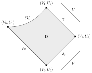
Figure 1: Picture of the domain of integration $D$ given a spacelike portion $\delta{\mathcal{H}}$ of the apparent horizon. In this case, $D\times\mathds{S}^{2}=J^{+}((V_{0},U_{0})\times\mathds{S}^{2})\cap J^{-}(\delta{\mathcal{H}}\times\mathds{S}^{2})$, with $U_{2}<U_{1}$. The initial data are posed on the curves $\rho_{0}$ and $\delta_{0}$ of the boundary $\partial D$.

With this definition of $D$ and with $S_{0}$ given by eq. (28), let us consider a stress-energy tensor $T_{\mu\nu}$ which respects the spherical symmetry and which satisfies the following initial conditions at the boundary of $J^{+}(S_{0})$:

$$T_{\mu\nu}(p)=0,\qquad p\in\partial J^{+}(S_{0}).$$ (32)

With the choice of $S_{0}\in\mathscr{I}^{-}(\Gamma)$, such an initial condition states that there is no influence of the matter in the past infinity. Then, applying the divergence theorem (Stokes’ theorem) to the current $J_{1}$ on the domain $D\times\mathds{S}^{2}$, following the derivation given in Appendix A.1, one obtains that

$${\Delta M}=-\left({\mathcal{S}}+{\mathcal{W}}\right),$$ (33)

where

$${\mathcal{S}} \doteq 2\pi\int_{D}\nabla\cdot J_{r}\mathrm{d}{\mathcal{V}}_{D},$$ (34)

$${\mathcal{W}} \doteq 4\pi\int_{\gamma}\frac{T_{UV}r^{2}}{A}(-\partial_{U}r)\mathrm{d}U.$$ (35)

Here $\mathrm{d}{\mathcal{V}}_{D}\doteq Ar^{2}\mathrm{d}V\wedge\mathrm{d}U$ denotes the volume form on $D$ in the $(V,U)$ plane. In particular, according to eqs. 33, 34 and 35, ${\mathcal{S}}$ is the matter source inside the domain $D$, whereas ${\mathcal{W}}$ is related to the component of $T_{\mu\nu}$ that is associated to the work $w$ done by the matter when evaluated on ${\mathcal{H}}$, in view of Hayward’s first law (18). In the next section we shall see how the quantum trace anomaly shown by the stress-energy tensor outside the black hole horizon forces $\mathcal{S}$ to be positive. We remark in passim that applying the divergence theorem to the current $J_{K}$ and comparing the result with eq. (33) yield ${\mathcal{R}}={\mathcal{S}}$, where

$${\mathcal{R}}\doteq 4\pi\int_{\gamma}\frac{T_{UU}r^{2}}{A}\partial_{V}r\mathrm{d}U$$ (36)

is related to the outgoing energy flux $T_{UU}$ across $\gamma$. Hence, in the case of stress-energy tensors satisfying ${\mathcal{W}}=0$ it follows that $\Delta M=-{\mathcal{R}}$. Finally, as before, the constraints on $\mathcal{S}$, that shall be imposed by the trace anomaly in the next section, force also the outgoing energy flux across $\gamma$ to be positive.

4 Evaporation induced by the quantum trace anomaly

In the previous section, eq. (33) showed that the ingoing energy flux $T_{VV}$ on the horizon together with $\Delta M$ are constrained by the matter content outside and in the causal past of the horizon, encoded in the source ${\mathcal{S}}$ and in the flux ${\mathcal{W}}$ given in eqs. 34 and 35 on the domain $D\times\mathds{S}^{2}$. Now, we shall see that a negative ingoing flux on the horizon, and thus the evaporation, can be obtained considering the non-vanishing trace anomaly of a quantum stress-energy tensor $\expectationvalue{{:}T_{\mu\nu}{:}}_{\omega}$. Actually, this anomalous trace forces ${\mathcal{S}}$ to be positive, and thus $\Delta M$ to be negative according to eq. (33), provided that an auxiliary averaged energy condition is also assumed to control ${\mathcal{W}}$.

For a free massless conformally coupled scalar field $\phi$, the non-vanishing trace of the quantum stress-energy tensor $\expectationvalue{{:}T_{\mu\nu}{:}}_{\omega}$ does not depend on the choice of the quantum state $\omega$, but it is fixed by the geometry of the spacetime to be equal to the quantum trace anomaly. In four dimensions, it reads

$$\expectationvalue{{:}{T_{\rho}}^{\rho}{:}}_{\omega}=\lambda\left({C_{\alpha\beta}}^{\gamma\delta}{C_{\gamma\delta}}^{\alpha\beta}+{R_{\mu}}^{\nu}{R_{\nu}}^{\mu}-\frac{1}{3}R^{2}\right),$$ (37)

where

$$\lambda\doteq\frac{1}{720(4\pi^{2})},$$ (38)

${C_{\alpha\beta}}^{\gamma\delta}$ is the Weyl tensor, ${R_{\mu}}^{\nu}$ the Ricci tensor and $R$ the Ricci scalar. The $\square R$ appearing e.g. in [Wal78] has been cancelled from eq. (37) by carefully choosing the renormalization freedoms inside the definition of $\expectationvalue{{:}{T_{\rho}}^{\rho}{:}}_{\omega}$. As discussed in [HW01, HW04], there is always enough freedom to remove higher order derivatives at the level of the trace. Actually, higher-order derivatives always appear in any renormalized quantum stress-energy tensor (see, e.g., the references given in the Section 1 about the computation of the stress-energy tensor in the Schwarzschild spacetime). These higher order derivatives could be eliminated at least at the level of the dynamical equations by imposing the consistency of the semiclassical theory as an expansion in $\hbar$ (see, e.g., [Sim91]). As in this paper we work only with the explicit form of the trace, we do not need to follow that way of reasoning and we simply use the renormalization freedom to remove higher order derivatives from the trace.

A quantum averaged weak energy condition is usually a non-local constraint of the form

$$\lim_{\lambda\to\infty}\inf\int f(t/\lambda)^{2}\expectationvalue{{:}T_{\mu\nu}{:}}_{\omega}k^{\mu}k^{\nu}(\gamma(t))\mathrm{d}t\geq 0$$ (39)

for any quantum state $\omega$ where $\expectationvalue{{:}T_{\mu\nu}{:}}_{\omega}$ can be evaluated. Here, $k^{\mu}$ is the tangent vector to the affine-parametrized timelike/null geodesic $\gamma(t)$ and $f$ is a real-valued smooth function having compact support on the domain of $\gamma$. It has been shown that this class of averaged energy conditions are valid both in flat and globally hyperbolic spacetimes for some values of the coupling parameter $\xi$, including the conformally coupled case (see [KS20] and references therein). Moreover, conditions like eq. (39) can also hold outside the limit and employing a specific sampling function for a restricted class of vacuum-like reference states. The sampling functions are often positive and smooth everywhere in their domain and also decay sufficiently fast at infinity. For instance, some common choices are Gaussian functions or compactly supported test functions having exponential decay in Fourier space, see, e.g., [FFR10, FF20, WFS21] and references therein. In our case, we shall employ an exponential smooth function $f(V,U)$ constructed from the geometry of the background, whose role is to tame those inside $\expectationvalue{{:}{T_{\rho}}^{\rho}{:}}_{\omega}$ which do not contribute to a negative variation of the mass $\Delta M$. Thus, the following theorem holds.

Theorem 4.1.

Consider a free quantum massless, conformally coupled scalar field $\phi$ propagating on a spherically symmetric dynamical background, whose metric, expressed according to eq. (6), solves the semiclassical Einstein equations (1) for a quantum state $\omega$. Suppose that $\omega$ is such that it makes the initial conditions stated in eq. (32) valid for the quantum stress-energy tensor $\expectationvalue{{:}T_{\mu\nu}{:}}_{\omega}$. Let

$$f(V,U)\doteq f_{0}(V)\exp(-8\pi\lambda\beta(V,U)),$$ (40)

where $\beta(V,U)$ is any solution of $\partial_{U}\beta(V,U)=\frac{2}{r}\partial_{V}r{R_{U}}^{V}$, and $f_{0}(V)=\exp{-k(V-V_{0})}$, for any $V\geq V_{0}$, is an exponentially decreasing function with a sufficiently large $k>0$. Let ${\Delta M}$ be given by eq. (22). If

$$\int_{U_{0}}^{U_{\mathcal{H}}}\frac{\expectationvalue{{:}T_{UV}{:}}_{\omega}r^{2}}{A}f(V,U)A\mathrm{d}U\geq 0$$ (41)

in the domain $\text{D}\times\mathds{S}^{2}$ defined in eqs. 30 and 31, for any $V\in[V_{0},V_{1}]$, (i.e., the integral in the left-hand side of the inequality is taken along any ingoing radial null curve connecting the initial point $(V,U_{0})$ and $(V,U_{\mathcal{H}})\in\delta{\mathcal{H}}$), then, ${\Delta M}<0$, namely the evaporation occurs along $\delta{\mathcal{H}}$.

Proof.

See the Appendix A.2 ∎

For a qualitative behaviour of $f(V,U)$ in some special cases, see Figure 2.

Figure 2: Plots of the qualitative behaviour of the smearing function $f(V,U)$ (40) at fixed $V=V_{1}$ for special choices of spacetime geometries. In the Schwarzschild and in the Vaidya spacetimes (${R_{\theta}}^{\theta}={R_{U}}^{V}=0$), $f$ is trivially a positive constant. In spacetimes where ${R_{\theta}}^{\theta}=0$ which are asymptotically flat (i.e., $\partial_{V}r/r$ decays as $U^{-1}$ and ${R_{U}}^{V}$ at least as $U^{-1}$ for large $U$), $f$ is bounded and greater than a strictly positive constant, and it approaches that constant for large $U$. In this respect, $f$ is similar to the sampling functions entering usual quantum averaged weak energy conditions (see, e.g., [FF20]).

At this stage, some remarks can be made about the formulation of Theorem 4.1. In this result, the quantum trace anomaly indeed drives the evaporation of the spherical black hole, because in the case of classical free matter field the initial conditions (32) would imply that the stress-energy tensor vanishes on $\partial D\times\mathds{S}^{2}$. Thus, eq. (41) would hold trivially and $\Delta M=0$, namely $\delta{\mathcal{H}}$ would be stable under the influence of the matter field. Moreover, the quantum averaged energy condition stated in the inequality (41) is compatible with the thermodynamic interpretation of $w=A^{-1}{T_{UV}}$ given by Hayward as the work done by the matter on the horizon, which is expected to be positive at least on its average. Also, we believe that this averaged condition can be formulated in more general terms and for a larger class of smooth functions $f(V,U)$, once a sufficiently well-behaved state $\omega$ has been chosen on spherically symmetric spacetimes. For instance, we can expect that such reference state fulfils also the averaged energy condition ${\mathcal{R}}>0$, where ${\mathcal{R}}$ was defined in eq. (36), with $\partial_{V}r$ as smearing function. In this case, the quantum outgoing flux $\expectationvalue{{:}T_{UU}{:}}_{\omega}$ could be interpreted as Hawking radiation emitted from the evaporating $\delta{\mathcal{H}}$ and sourced by the trace anomaly inside ${\mathcal{S}}$. Unfortunately, the lack of control on the evolution of a quantum state $\omega$ which was a vacuum in the past, namely satisfying eq. (32), prevents us to formulate explicitly a general quantum energy condition compatible with all the previous statements.

However, we expect that the condition (41) is fulfilled at least in an approximate way in the causal past. Actually, classical solutions are approximately valid in semiclassical gravity, because quantum corrections are small outside the horizon. Under this approximation, the condition (41) is often satisfied - even pointwise - in the most realistic spherically symmetric models of collapse, where the classical matter sourcing the background fulfils the dominant energy condition $A^{-1}T_{UV}\geq 0$. As examples, we can think at the Lemaître-Tolman-Bondi models like the Oppenheimer-Snyder solution, where the collapse is driven by an (in)homogeneous spherical cloud of dust at zero pressure satisfying the weak energy condition, see, e.g., [GP09] and references therein. Furthermore, in Christodoulou’s work about the collapse in the case of matter described by a classical scalar field [Chr86a, Chr86b, Chr91] the collapsing matter is described by a classical massless scalar field $\phi$ that is invariant under rotations and having stress-energy tensor given by $T_{\mu\nu}=\partial_{\mu}\phi\partial_{\nu}\phi-\frac{1}{2}g_{\mu\nu}\partial_{\rho}\phi\partial^{\rho}\phi$. Hence, $T_{UV}=0$ and the dominant energy condition holds again.

There are two special backgrounds fulfilling $T_{UV}=0$ from the Einstein equation $G_{UV}=8\pi T_{UV}=0$, namely the Schwarzschild and the Vaidya spacetimes. The former describes a static spherically symmetric black hole, while the latter defines the geometry outside a null radiating star, see, e.g., [GP09] and references therein. In Bardeen-Vaidya parametrization (4), the Schwarzschild and the Vaidya metrics are obtained by choosing $m\in\mathds{R}^{+}$ and $m=m(v)$, respectively, and by fixing $\Psi(v,r)=0$. In these cases, the semiclassical regime where $R_{\mu\nu\rho\sigma}R^{\mu\nu\rho\sigma}\ll m_{P}^{4}$ is always satisfied for $m/m_{P}\gg(3/4)^{1/4}\simeq 0.93$, which holds for astrophysical masses (for a solar mass, $M_{\astrosun}/m_{P}\simeq 10^{38}$). In the Vaidya spacetime, the trace anomaly reads

$$\expectationvalue{{:}{T_{\rho}}^{\rho}{:}}_{\omega}=48\lambda\frac{M(v)^{2}}{r^{6}},$$ (42)

where $\lambda$ is the coefficient (38). In this case the rate of evaporation can be directly computed using eq. (23) after evaluating the negative ingoing flux $\expectationvalue{{:}T_{VV}{:}}_{\omega}$ on ${\mathcal{H}}$. To obtain $\expectationvalue{{:}T_{VV}{:}}_{\omega}$, we employ the conservation equation $\nabla^{\mu}\expectationvalue{{:}T_{\mu V}{:}}_{\omega}=0$, which yields

$$-\frac{1}{Ar^{2}}\partial_{U}\left(\expectationvalue{{:}T_{VV}{:}}_{\omega}r^{2}\right)-\frac{1}{r^{2}}\partial_{V}\left(A^{-1}\expectationvalue{{:}T_{UV}{:}}_{\omega}r^{2}\right)-2\expectationvalue{{:}{T_{\theta}}^{\theta}{:}}_{\omega}\frac{\partial_{V}r}{r}=0,$$

where

$$\expectationvalue{{:}{T_{\theta}}^{\theta}{:}}_{\omega}=\frac{\expectationvalue{{:}T_{UV}{:}}_{\omega}}{A}+\frac{1}{2}\expectationvalue{{:}{T_{\rho}}^{\rho}{:}}_{\omega}.$$ (43)

It is usually very challenging to evaluate the renormalized quantum stress-energy tensor on a state which is a vacuum state in the past. Furthermore, contrary to its classical counterpart (see, e.g., [DFU76] for the two-dimensional case), $\expectationvalue{{:}T_{UV}{:}}_{\omega}$ is expected not to vanish in a generic quantum state $\omega$, and hence Vaidya spacetime is not expected to be a full solution of the semiclassical equations. Here, we shall assume for simplicity that there exists a quantum state $\omega$ in which $\expectationvalue{{:}T_{UV}{:}}_{\omega}=0$ and which makes Vaidya spacetime a semiclassical solution outside the horizon. With this assumption, the ingoing flux fulfils the following differential equation in $(v,r)$ coordinates

$$\partial_{r}(\expectationvalue{{:}T_{VV}{:}}_{\omega}r^{2})=24\lambda M(v)^{2}\left(\frac{1}{r^{5}}-\frac{2M(v)}{r^{6}}\right).$$

Integrating in $(r_{\mathcal{H}},\infty)$, imposing the initial condition $\expectationvalue{{:}T_{VV}{:}}_{\omega}r^{2}\rightarrow 0$ when $r\rightarrow\infty$, and changing sign, the ingoing flux reads

$$\expectationvalue{{:}T_{VV}{:}}_{\omega}r^{2}\stackrel{{\scriptstyle\mbox{\tiny${\mathcal{H}}$}}}{{=}}-24\lambda M^{2}\int_{r_{\mathcal{H}}}^{+\infty}\left(\frac{1}{r^{5}}-\frac{2M(v)}{r^{6}}\right)\mathrm{d}r=-\frac{3\lambda}{40M(v)^{2}}.$$ (44)

Hence, the rate of evaporation obtained from eq. (23) is

$$\dot{M}(v)=-\frac{3\pi\lambda}{10M(v)^{2}}.$$ (45)

Eq. (45) is an ordinary differential equation with respect to $v$ and it can be integrated by separation of variables, yielding the evaporation law

$$M^{3}(v)=M_{0}^{3}-\frac{9\pi\lambda}{10}(v-v_{0}),$$ (46)

where we have defined the total initial mass $M_{0}\doteq M(v_{0})$ at the initial time $v_{0}$. Thus, the evaporation process is completed in the time interval $\Delta v\doteq v-v_{0}=10M_{0}^{3}/(9\pi\lambda)$. Moreover, according to the first law given in (18) for the Vaidya spacetime, the negative rate (45) induces also a shrink of the area of the horizon ${\mathcal{A}}_{\mathcal{H}}$, whose rate of variation $\dot{{\mathcal{A}}}_{\mathcal{H}}(v)\doteq\partial_{v}{\mathcal{A}}(v,r_{\mathcal{H}}(v))$ is governed by $\dot{M}(v)=(\kappa/8\pi)\dot{{\mathcal{A}}}_{\mathcal{H}}(v)$. Hence, a negative variation of the Wald-Kodama dynamical entropy $S_{\mathcal{H}}\doteq{\mathcal{A}}_{\mathcal{H}}/4$ [AH99, HMA99] holds, namely

$$\frac{\mathrm{d}S_{\mathcal{H}}(v)}{\mathrm{d}v}=-\frac{12\pi^{2}\lambda}{5M(v)}.$$ (47)

Therefore, it follows that the Schwarzschild spacetime is not a solution of the semiclassical Einstein equations, because the variation of the mass trivially vanishes in the case of constant mass. This prevents to obtain an equation for the rate like eq. (45) in the static case. Hence, an eternal black hole cannot be in equilibrium with the back-reaction of any quantum matter field outside the horizon which is in a vacuum state in the asymptotic causal past.

The only quantum property of matter which was used to obtain black hole evaporation is the anomalous contribution to the trace of the quantum matter stress-energy tensor. Hence, an immediate generalization of the foregoing argument may be carried out by extending the analysis to arbitrary massless conformally coupled fields, after modifying the coefficient $\lambda$ inside the trace anomaly given in eq. (37). In the general case, the four-dimensional anomalous trace is given by $\expectationvalue{{:}{T_{\rho}}^{\rho}{:}}_{\omega}=b_{F}F+b_{G}G$, where $F=C_{\alpha\beta\gamma\delta}C^{\alpha\beta\gamma\delta}$ is the square of the Weyl tensor, $G=R_{\mu\nu\rho\sigma}R^{\mu\nu\rho\sigma}-4R_{\mu\nu}R^{\mu\nu}+R^{2}$ is the Euler density and $b_{F}$, $b_{G}$ are coefficients depending on the numbers of particles $n_{s}$ of spin $s$. For the explicit values of $b_{F}$ and $b_{G}$, see [BD84]. Arguably, a generalization of the Theorem 4.1 can be obtained for arbitrary fields after choosing properly the coefficients inside $\expectationvalue{{:}{T_{\rho}}^{\rho}{:}}_{\omega}$. Further generalizations of the analysis presented in this paper beyond the spherically symmetric case are harder to obtain.

5 Conclusion

The understanding of the mechanism that leads to the evaporation of a (spherically symmetric) black hole is totally within the scope of semiclassical gravity. It turns out that the negative variation of the black hole mass is due to a negative ingoing flux on the horizon. Such a flux can be obtained by modelling matter outside and in the causal past of the horizon as a conformally coupled quantum scalar field. This model clearly shows that the key of evaporation is the quantum trace anomaly for suitable vacuum-like initial conditions in the past. Of course, to overcome the poor control on the state-dependent contribution to the stress-energy tensor in the dynamical case, some energy condition should be assumed, and here we made a choice which facilitates the analysis and is satisfied in known models of gravitational collapse. As an example, we have computed the rate of evaporation explicitly in the Vaidya spacetime and shown that the Schwarzschild spacetime can never be in equilibrium with the quantum matter field outside the horizon, if the quantum matter is in a state which is the vacuum in the asymptotic past.

The results obtained here should be regarded as a first step towards a more complete analysis of black hole evaporation in semiclassical gravity. A full solution of the semiclassical Einstein equations showing black hole evaporation is still lacking. This solution is available only in the two-dimensional case [APR11b, APR11a]. The difficulties in controlling the state-dependent contributions in the expectation values of the stress-energy tensor prevent the generalization to the four-dimensional case. In this regard, a study similar to the one in [MPS20] for cosmological spacetimes would be desirable.

Acknowledgements

We thank two anonymous referees for helpful comments on an earlier version of this paper.

Appendix A Appendix

A.1 Proof of eq. (33)

Using that $T^{UV}=A^{-2}T_{UV}$ and $T^{UU}=A^{-2}T_{VV}$ we can relate the current $J_{1}$ defined in eq. (26) to the variation of the mass (22) computed along the line enclosed between $(V_{0},U_{1}),(V_{1},U_{2})\in\delta{\mathcal{H}}$ in the $(V,U)$ plane (see Figure 1). In $(V,U)$ coordinates, the derivatives of the Misner-Sharp energy (3) read

$$\partial_{V}m=\frac{4\pi r^{2}}{A}\left({T_{UV}}\partial_{V}r-{T_{VV}}\partial_{U}r\right),$$ (48a)

$$\partial_{U}m=\frac{4\pi r^{2}}{A}\left({T_{UV}}\partial_{U}r-{T_{UU}}\partial_{V}r\right).$$ (48b)

Evaluating eqs. (48a) and (48b) on $\partial_{V}r\stackrel{{\scriptstyle\mbox{\tiny${\mathcal{H}}$}}}{{=}}0$, we obtain that

$${\Delta M}=4\pi\int_{\delta{\mathcal{H}}}r^{2}(-\partial_{U}r)\left(\frac{{T_{VV}}}{A}\mathrm{d}V-\frac{{T_{VU}}}{A}\right)\mathrm{d}U=4\pi\int_{\delta{\mathcal{H}}}Ar^{2}\left(J_{1}^{V}\mathrm{d}U-J_{1}^{U}\mathrm{d}V\right).$$ (49)

Eq. (33) can be obtained by applying the divergence theorem (Stokes’ theorem) to the current $J_{1}$ on the domain $D\times\mathds{S}^{2}$. Using the spherical symmetry to integrate out the angular variables $(\varphi,\theta)$, we obtain that

$$-\int_{D}\left(\nabla\cdot J_{1}\right)\mathrm{d}{\mathcal{V}}_{D} =\int_{\delta{\mathcal{H}}}(J_{1}^{V}Ar^{2}\mathrm{d}U-J_{1}^{U}Ar^{2}\mathrm{d}V)+\int_{\rho_{0}}J_{1}^{V}Ar^{2}\mathrm{d}U+\int_{\delta_{0}}J_{1}^{U}Ar^{2}\mathrm{d}V-\int_{\gamma}J_{1}^{V}Ar^{2}\mathrm{d}U.$$

With the choice of the initial conditions (32), both the integrals along $\rho_{0}$ and $\delta_{0}$ vanish. By substitution of eq. (49) at the place of the integral over $\delta{\mathcal{H}}$, we get

$$-\int_{D}\left(\nabla\cdot J_{1}\right)\mathrm{d}{\mathcal{V}}_{D}=\frac{\Delta M}{4\pi}-\int_{U_{0}}^{U_{2}}Ar^{2}J_{1}^{V}\mathrm{d}U.$$

Thus, eq. (33) is obtained by employing the definition $J_{1}=(J_{r}-J_{K})/2$, where $J_{r}$ and $J_{K}$ are given in eqs. (26) and (27), and by using that $\nabla\cdot J_{1}=\frac{1}{2}\nabla\cdot J_{r}$, since $\nabla\cdot J_{K}=0$ everywhere.

A.2 Proof of Theorem 4.1

The proof consists in applying the divergence theorem (Stokes’ theorem) on the domain $D\times\mathds{S}^{2}$ to a quantum current $\tilde{J}$ depending on $\expectationvalue{{:}T_{\mu\nu}{:}}_{\omega}$, which is a weighted version of $J_{1}$ given in eqs. 26 and 27. The weight is given in terms of a strictly positive function $f(V,U)$ which will be fixed later. Let us define

$$\tilde{J}_{\mu}\doteq\xi^{\nu}\expectationvalue{{:}T_{\nu\mu}{:}}_{\omega},\qquad\xi^{\nu}=f(V,U)(\partial_{V})^{\nu}$$

and the weighted variation of the mass

$$\Delta_{h}M\doteq\int_{\delta{\mathcal{H}}}h\mathrm{d}m$$ (50)

with respect to the function

$$h(V,U)\doteq\frac{f(V,U)A(V,U)}{-\partial_{U}r(V,U)}.$$ (51)

The divergence of $\tilde{J}$ is related to the variation of the weighted mass (50) by the following equation:

$$\Delta_{h}M=-4\pi\int_{D}\nabla\cdot\tilde{J}\mathrm{d}{\mathcal{V}}_{D}-4\pi\int_{U_{0}}^{U_{2}}\frac{\expectationvalue{{:}T_{UV}{:}}_{\omega}}{A}fAr^{2}\mathrm{d}U,$$ (52)

where

$$\Delta_{h}M=4\pi\int_{\delta{\mathcal{H}}}r^{2}\left(\tilde{J}_{V}\mathrm{d}V-\tilde{J}_{U}\mathrm{d}U\right).$$

Eq. (52) can be obtained similarly to what already done in the Appendix A.1 for the current $J_{1}$, namely by applying the divergence theorem (Stokes’ theorem) to the weighted current $\tilde{J}_{\mu}$ on the domain $D\times\mathds{S}^{2}$, under the assumptions of Section 3 for the domain $D$ and imposing the initial conditions (32) on $\expectationvalue{{:}T_{\mu\nu}{:}}_{\omega}$.

Using the conservation equation $\nabla^{\mu}\expectationvalue{{:}T_{\mu\nu}{:}}_{\omega}=0$, the relation (43), and the semiclassical equations $A^{-1}\expectationvalue{{:}T_{UV}{:}}_{\omega}={R_{\theta}}^{\theta}/(8\pi)$, $A^{-1}\expectationvalue{{:}T_{VV}{:}}_{\omega}=-{R_{V}}^{U}/(8\pi)$,

$$\nabla\cdot\tilde{J}=\frac{1}{8\pi}\left[-\left(-{R_{V}}^{U}\partial_{U}f+{R_{\theta}}^{\theta}\partial_{V}f\right)+f\left(-{R_{\theta}}^{\theta}\frac{\partial_{V}A}{A}+2{R_{\theta}}^{\theta}\frac{\partial_{V}r}{r}+8\pi\expectationvalue{{:}{T_{\rho}}^{\rho}{:}}_{\omega}\frac{\partial_{V}r}{r}\right)\right].$$

Here, $\expectationvalue{{:}{T_{\rho}}^{\rho}{:}}_{\omega}$ is a geometric quantity given in terms of the trace anomaly in eq. (37). There we can isolate a positive contribution after computing explicitly the product

$${C_{\alpha\beta}}^{\gamma\delta}{C_{\gamma\delta}}^{\alpha\beta}=\left(R+\frac{12\kappa}{r}\right)^{2}=4\left({R_{U}}^{U}+{R_{\theta}}^{\theta}+\frac{6\kappa}{r}\right)^{2}$$

and the difference

$${R_{\mu}}^{\nu}{R_{\nu}}^{\mu}-\frac{1}{3}R^{2}=2{R_{V}}^{U}{R_{U}}^{V}+\frac{2}{3}\left(({R_{U}}^{U})^{2}+\left({R_{\theta}}^{\theta}\right)^{2}\right)-\frac{8}{3}{R_{\theta}}^{\theta}{R_{U}}^{U}.$$

Hence, the anomaly can be rewritten as

$$\expectationvalue{{:}{T_{\rho}}^{\rho}{:}}_{\omega}=\lambda\left(4\left({R_{U}}^{U}+{R_{\theta}}^{\theta}+\frac{6\kappa}{r}\right)^{2}+\frac{2}{3}\left(({R_{U}}^{U})^{2}+\left({R_{\theta}}^{\theta}\right)^{2}\right)+2{R_{V}}^{U}{R_{U}}^{V}-\frac{8}{3}{R_{U}}^{U}{R_{\theta}}^{\theta}\right),$$

where the first two terms are manifestly positive. Plugging this expression inside eq. (52) yields

$$\Delta_{h}M =-4\pi\lambda\int_{\text{D}}\left(4\left({R_{U}}^{U}+{R_{\theta}}^{\theta}+\frac{6\kappa}{r}\right)^{2}+\left(({R_{U}}^{U})^{2}+\left({R_{\theta}}^{\theta}\right)^{2}\right)\right)\frac{\partial_{V}r}{r}f\mathrm{d}{\mathcal{V}}_{\text{D}}$$ (53)

$$-4\pi\int_{\text{D}}\left(-\frac{\partial_{V}f}{f}+\partial_{V}\log(A^{-1}r^{2})-\lambda\frac{64\pi}{3}{R_{U}}^{U}\frac{\partial_{V}r}{r}\right){\frac{{R_{\theta}}^{\theta}}{8\pi}}f\mathrm{d}{\mathcal{V}}_{\text{D}}$$

$$-4\pi\int_{\text{D}}\left({+}\frac{\partial_{U}f}{f}+{8\pi}\lambda\frac{2\partial_{V}r}{r}{{R_{U}}^{V}}\right){\frac{{R_{V}}^{U}}{8\pi}}f\mathrm{d}{\mathcal{V}}_{\text{D}}-4\pi\int_{U_{0}}^{U_{2}}\frac{\expectationvalue{{:}T_{UV}{:}}_{\omega}r^{2}}{A}f(V_{1},U)A\mathrm{d}U.$$

Since $D$ is a normal domain, e.g., with respect to the $V$-axis for any ${\mathcal{F}}(V,U)\in{\mathcal{C}}^{\infty}({\mathcal{M}})$, it holds that

$$\int_{D}{\mathcal{F}}(V,U)\mathrm{d}{\mathcal{V}}_{D}=\int_{V_{0}}^{V_{1}}\mathrm{d}V\int_{U_{0}}^{U_{{\mathcal{H}}}(V)}{\mathcal{F}}(V,U)Ar^{2}\mathrm{d}U,$$ (54)

where $U_{{\mathcal{H}}}(V)$ is the solution of $2r(V,U)-m(V,U)=0$.

Our aim is to prove now that $\Delta_{h}M$ is strictly negative using eq. (53). To this aim, we shall isolate all the integrals in the right-hand side which give a negative contribution to $\Delta_{h}M$, while we tame the effects of the other choosing carefully the geometric function $f$. Actually, we want to find a function $f(V,U)>0$ such that all these unwanted terms in eq. (53) vanish. Let $\beta(V,U)$ be any fixed primitive function of

$$\partial_{U}\beta(V,U)=\frac{2}{r}\partial_{V}r{{R_{U}}^{V}},$$

The $U$-derivative of $f$ is fixed in such a way to cancel the volume integral whose integrand is proportional to ${R_{V}}^{U}$, namely it must be a solution of the equation

$$\left(\frac{\partial_{U}f}{f}+{8\pi}\lambda\frac{2\partial_{V}r}{r}{{R_{U}}^{V}}\right)=0.$$

Hence, we get

$$f(V,U)=f_{0}(V)\exp({-8\pi}\lambda\beta(V,U)),$$

where $f_{0}(V)$ is an integration constant which can be chosen consistently with the hypothesis stated in the Theorem. Plugging this function $f(V,U)$ in the contributions of eq. (53) yields

$$\Delta_{h}M= -4\pi\int_{V_{0}}^{V_{1}}{f_{0}}(V)\;(\gamma_{3}(V)+\gamma_{1}(V))\mathrm{d}V+4\pi\int_{V_{0}}^{V_{1}}{\partial_{V}f_{0}}(V)\;\gamma_{2}(V)\mathrm{d}V$$ (55)

$$-4\pi\int_{U_{0}}^{U_{2}}\frac{\expectationvalue{{:}T_{UV}{:}}_{\omega}r^{2}}{A}f(V_{1},U)A\mathrm{d}U,$$

where

$$\gamma_{1}(V) =\frac{1}{8\pi}\int_{U_{0}}^{U_{{\mathcal{H}}}}{R_{\theta}}^{\theta}\left(\partial_{V}\log(A^{-1}r^{2})+8\pi\lambda\left(-\frac{8}{3}{R_{U}}^{U}\frac{\partial_{V}r}{r}+\partial_{V}\beta(V,U)\right)\right)\frac{f}{f_{0}}Ar^{2}\mathrm{d}\tilde{U},$$

$$\gamma_{2}(V) =\frac{1}{8\pi}\int_{U_{0}}^{U_{{\mathcal{H}}}}{R_{\theta}}^{\theta}\frac{f}{f_{0}}Ar^{2}\mathrm{d}\tilde{U},$$

and $\gamma_{3}$ is

$$\gamma_{3}(V)=\lambda\int_{U_{0}}^{U_{{\mathcal{H}}}(V)}\left(4\left({R_{U}}^{U}+{R_{\theta}}^{\theta}+\frac{6\kappa}{r}\right)^{2}+\frac{2}{3}\left(({R_{U}}^{U})^{2}+({R_{\theta}}^{\theta})^{2}\right)\right)\frac{\partial_{V}r}{r}\frac{f}{f_{0}}Ar^{2}\mathrm{d}\tilde{U}.$$

To prove that $\Delta_{h}M$ is strictly negative, the three contributions given by the three integrals on the right hand side of eq. (55) are analyzed separately. Since $\partial_{V}r>0$ outside the horizon, $\gamma_{3}$ can be controlled as follows:

$$\gamma_{3}(V)\geq\frac{144}{13}\lambda\int_{U_{0}}^{U_{{\mathcal{H}}}(V)}\kappa^{2}\frac{\partial_{V}r}{r}\frac{f}{f_{0}}A\mathrm{d}U.$$

From the behaviour on the apparent horizon of the expansion parameters of the ingoing and outgoing radial null geodesics given in eq. (10), and according to the definition of $\kappa$ given in (17), $\kappa$ is strictly positive on the apparent horizon, and by continuity it stays positive also near the horizon. Thus, $\gamma_{3}(V)$ is strictly positive for $V\in[V_{0},V_{1}]$.

Moreover, the initial conditions given on the hypersurface $\rho_{0}$ which is part of $\partial D$ imply that ${R_{\theta}}^{\theta}=A^{-1}\expectationvalue{{:}T_{UV}{:}}_{\omega}=0$ on $\rho_{0}$, and hence $\gamma_{1}(V_{0})=\gamma_{2}(V_{0})=0$. Then, $\gamma_{1}+\gamma_{3}$ is strictly positive for $V=V_{0}$, and by continuity it stays strictly positive also for $V$ near $V_{0}$. Therefore, we may find a constant $\delta>0$ such that $f_{0}(\gamma_{3}+\gamma_{1})$ is strictly positive on $[V_{0},V_{0}+\delta]$. If $k$ in $f_{0}$ is sufficiently large, the integral of $f_{0}(\gamma_{3}+\gamma_{1})$ over $[V_{0},V_{1}]$ is dominated by the contribution on $[V_{0},V_{0}+\delta]$. Hence, the first contribution in the right-hand side of eq. (55) containing $\gamma_{3}+\gamma_{1}$ is strictly negative for that choice of $k$.

Furthermore, the term containing $\gamma_{2}$ in $\Delta_{h}M$ in eq. (55) is negative or null, because $\partial_{V}f_{0}<0$ on $[V_{0},V_{1}]$, ${R_{\theta}}^{\theta}=A^{-1}\expectationvalue{{:}T_{UV}{:}}_{\omega}=0$, and $\gamma_{2}(V)\geq 0$ for all $V\in[V_{0},V_{1}]$, according to the hypothesis stated in eq. (41).

Finally, the condition (41) also implies that the last integral appearing in $\Delta_{h}M$ in eq. (55), which is computed for $V\in V_{1}$ and supported in $[U_{0},U_{2}]$, gives a negative (or null) contribution to $\Delta_{h}M$.

Taking into account all this and with this choice of $f(V,U)$, $h(V,U)$ given in eq. (51) is also positive and smooth. Hence, it is bounded from below in $\delta{\mathcal{H}}$, so $0>\Delta_{h}M\geq C{\Delta M}$, where $C>0$, and the proof of the Theorem holds.

References

- [AV10] G. Abreu and M. Visser, “Kodama time: Geometrically preferred foliations of spherically symmetric spacetimes,” Phys. Rev. D 82, 044027 (2010) [10.1103/PhysRevD.82.044027]
- [AGCF20] P. R. Anderson, S. Gholizadeh Siahmazgi, R. D. Clark, and A. Fabbri, “Method to compute the stress-energy tensor for a quantized scalar field when a black hole forms from the collapse of a null shell,” Phys. Rev. D 102(12), 125035 (2020) [10.1103/PhysRevD.102.125035]
- [AHS95] P. R. Anderson, W. A. Hiscock, and D. A. Samuel, “Stress-energy tensor of quantized scalar fields in static spherically symmetric spacetimes,” Phys. Rev. D 51, 4337 (1995) [10.1103/PhysRevD.51.4337]
- [AK02] A. Ashtekar and B. Krishnan, “Dynamical horizons: Energy, angular momentum, fluxes and balance laws,” Phys. Rev. Lett. 89, 261101 (2002) [10.1103/PhysRevLett.89.261101]
- [AK03] A. Ashtekar and B. Krishnan, “Dynamical horizons and their properties,” Phys. Rev. D 68, 104030 (2003) [10.1103/PhysRevD.68.104030]
- [AK04] A. Ashtekar and B. Krishnan, “Isolated and dynamical horizons and their applications,” Liv. Rev. Rel. 7, 10 (2004) [10.12942/lrr-2004-10]
- [APR11a] A. Ashtekar, F. Pretorius, and F. M. Ramazanoglu, “Evaporation of 2-Dimensional Black Holes,” Phys. Rev. D 83, 044040 (2011) [10.1103/PhysRevD.83.044040]
- [APR11b] A. Ashtekar, F. Pretorius, and F. M. Ramazanoglu, “Surprises in the Evaporation of 2-Dimensional Black Holes,” Phys. Rev. Lett. 106, 161303 (2011) [10.1103/PhysRevLett.106.161303]
- [AH99] M. C. Ashworth and S. A. Hayward, “Boundary terms and Noether current of spherical black holes,” Phys. Rev. D 60, 084004 (1999) [10.1103/PhysRevD.60.084004]
- [Bal84] R. Balbinot, “Hawking radiation and the back reaction-a first approach,” Class. Quant. Grav. 1(5), 573 (1984) [10.1088/0264-9381/1/5/010]
- [BB89] R. Balbinot and A. Barletta, “The backreaction and the evolution of quantum black holes,” Class. Quant. Grav. 6(2), 195 (1989) [10.1088/0264-9381/6/2/013]
- [Bar81] J. M. Bardeen, “Black holes do evaporate thermally,” Phys. Rev. Lett. 46(6), 382 (1981) [10.1103/PhysRevLett.46.382]
- [Bar14] J. M. Bardeen, “Black hole evaporation without an event horizon,” (2014) [arXiv:1406.4098 [gr-qc]]
- [BD84] N. D. Birrell and P. C. W. Davies, Quantum fields in curved space 7. Cambridge University Press, 1984.
- [Brow18] P. J. Brown, C. J. Fewster, and E. A. Kontou, “A singularity theorem for Einstein–Klein–Gordon theory,” Gen. Rel. Grav. 50, 121 (2018) [10.1007/s10714-018-2446-5]
- [BFK96] R. Brunetti, K. Fredenhagen, and M. Köhler, “The microlocal spectrum condition and Wick polynomials of free fields on curved spacetimes,” Commun. Math. Phys. 180(3), 633 (1996) [10.1007/s00220-003-0815-7]
- [Can80] P. Candelas, “Vacuum polarization in Schwarzschild space-time,” Phys. Rev. D 21, 2185 (1980) [10.1103/PhysRevD.21.2185]
- [Cas04] R. Casadio, “Holography and trace anomaly: What is the fate of (brane-world) black holes?,” Phys. Rev. D 69, 084025 (2004) [10.1103/PhysRevD.69.084025]
- [CF77] S. M. Christensen and S. A. Fulling, “Trace Anomalies and the Hawking Effect,” Phys. Rev. D 15, 2088 (1977) [10.1103/PhysRevD.15.2088]
- [Chr86a] D. Christodoulou, “Global existence of generalized solutions of the spherically symmetric Einstein-scalar equations in the large,” Commun. Math. Phys. 106(4), 587 (1986) [10.1007/BF01463398]
- [Chr86b] D. Christodoulou, “The problem of a self-gravitating scalar field,” Commun. Math. Phys. 105(3), 337 (1986) [10.1007/BF01205930]
- [Chr91] D. Christodoulou, “The formation of black holes and singularities in spherically symmetric gravitational collapse,” Commun. Pure Appl Math. 44(3), 339 (1991) [10.1002/cpa.3160440305]
- [DFU76] P. C. W. Davies, S. A. Fulling, and W. G. Unruh, “Energy-momentum tensor near an evaporating black hole,” Phys. Rev. D 13, 2720 (1976) [10.1103/PhysRevD.13.2720]
- [DNVZZ07] R. Di Criscienzo, M. Nadalini, L. Vanzo, S. Zerbini, and G. Zoccatelli, “On the Hawking radiation as tunneling for a class of dynamical black holes,” Phys. Let. B 657, 107 (2007) [10.1016/j.physletb.2007.10.005]
- [E19] V. A. Emelyanov, “Black-Hole Evolution from Stellar Collapse,” Fortsch. Phys. 67(5), 1800114 (2019) [10.1002/prop.201800114]
- [FF20] C. J. Fewster and L. H. Ford, “Probability Distributions for Space and Time Averaged Quantum Stress Tensors,” Phys. Rev. D 101, 025006 (2020) [10.1103/PhysRevD.101.025006]
- [FFR10] C. J. Fewster, L. H. Ford and T. A. Roman, “Probability distributions of smeared quantum stress tensors,” Phys. Rev. D 81, 121901 (2010) [10.1103/PhysRevD.81.121901]
- [FK20] C. J. Fewster and E. A. Kontou, “A new derivation of singularity theorems with weakened energy hypotheses,” Class. Quant. Grav. 37(6), 065010 (2020) [10.1088/1361-6382/ab685b]
- [FR03] C. J. Fewster and T. A. Roman, “Null energy conditions in quantum field theory,” Phys. Rev. D 67, 044003 (2003) [10.1103/PhysRevD.67.044003] [Erratum: Phys.Rev.D 80, 069903 (2009)]
- [FV03] C. J. Fewster and R. Verch, “Stability of quantum systems at three scales: Passivity, quantum weak energy inequalities and the microlocal spectrum condition,” Commun. Math. Phys. 240, 329 (2003) [10.1007/s00220-003-0884-7]
- [Fla97] E. E. Flanagan, “Quantum inequalities in two-dimensional Minkowski space-time,” Phys. Rev. D 56, 4922 (1997) [10.1103/PhysRevD.56.4922]
- [FR95] L. H. Ford and T. A. Roman, “Averaged energy conditions and quantum inequalities,” Phys. Rev. D 51, 4277 (1995) [10.1103/PhysRevD.51.4277]
- [FR96] L. H. Ford and T. A. Roman, “Averaged energy conditions and evaporating black holes,” Phys. Rev. D 53, 1988 (1996) [10.1103/PhysRevD.53.1988]
- [FR97] L. H. Ford and T. A. Roman, “Restrictions on negative energy density in flat space-time,” Phys. Rev. D 55, 2082 (1997) [10.1103/PhysRevD.55.2082]
- [FH90] K. Fredenhagen and R. Haag, “On the derivation of Hawking radiation associated with the formation of a black hole,” Commun. Math. Phys. 127(2), 273 (1990) [10.1007/BF02096757]
- [FKK20] B. Freivogel, E. A. Kontou, and D. Krommydas, “The return of the singularities: Applications of the smeared null energy condition,” (2020) [arXiv: 2012.11569 [gr-qc]]
- [FD76] S. A. Fulling and P. C. W. Davies, “Radiation from a moving mirror in two dimensional space-time: conformal anomaly,” Proc. Roy. Soc. A 348(1654), 393 (1976) [10.1098/rspa.1976.0045]
- [GP09] J. B. Griffiths and J. Podolsky, Exact Space-Times in Einstein’s General Relativity Cambridge Monographs on Mathematical Physics. Cambridge University Press, Cambridge, 2009. [10.1017/CBO9780511635397]
- [Haw68] S. W. Hawking, “Gravitational radiation in an expanding universe,” J. Math. Phys. 9, 598 (1968) [10.1063/1.1664615]
- [Haw74] S. W. Hawking, “Black hole explosions?” Nature 248(5443), 30 (1974) [10.1038/248030a0]
- [Haw75] S. W. Hawking, “Particle creation by black holes,” Commun. Math. Phys. 43(3), 199 (1975) [10.1007/BF02345020]
- [HDVNZ09] S. Hayward, R. Di Criscienzo, L. Vanzo, M. Nadalini, and S. Zerbini, “Local Hawking temperature for dynamical black holes,” Class. Quant. Grav. 26, 062001 (2009) [10.1088/0264-9381/26/6/062001]
- [Hay93] S. A. Hayward, “General laws of black-hole dynamics,” Phys. Rev. D 49, 6467 (1994)
- [Hay96] S. A. Hayward, “Gravitational energy in spherical symmetry,” Phys. Rev. D 53(6), 1938 (1996) [10.1103/PhysRevD.53.1938]
- [Hay98] S. A. Hayward, “Unified first law of black hole dynamics and relativistic thermodynamics,” Class. Quant. Grav. 15, 3147 (1998) [10.1088/0264-9381/15/10/017]
- [Hay00] S. A. Hayward, “Black holes: New horizons,” In “9th Marcel Grossmann Meeting on Recent Developments in Theoretical and Experimental General Relativity, Gravitation and Relativistic Field Theories (MG 9),” pages 568–580. 2000. [10.1088/0264-9381/26/6/062001]
- [HMA99] S. A. Hayward, S. Mukohyama, and M. C. Ashworth, “Dynamic black-hole entropy,” Phys. Let. A 256(5), 347 (1999) ISSN 0375-9601. [10.1016/S0375-9601(99)00225-X]
- [HW01] S. Hollands and R. M. Wald, “Local Wick polynomials and time ordered products of quantum fields in curved space-time,” Commun. Math. Phys. 223, 289 (2001) [10.1007/s002200100540]
- [HW02] S. Hollands and R. M. Wald, “Existence of local covariant time ordered products of quantum fields in curved space-time,” Commun. Math. Phys. 231, 309 (2002) [10.1007/s00220-002-0719-y]
- [HW04] S. Hollands and R. M. Wald, “Conservation of the stress tensor in interacting quantum field theory in curved spacetimes,” Rev. Math. Phys. 17, 227 (2005) [10.1142/S0129055X05002340]
- [HW15] S. Hollands and R. M. Wald, “Quantum fields in curved spacetime,” Physics Reports 574, 1 (2015) [10.1016/j.physrep.2015.02.001]
- [How84] K. W. Howard, “Vacuum in Schwarzschild spacetime,” Phys. Rev. D 30, 2532 (1984) [10.1103/PhysRevD.30.2532]
- [KW91] B. S. Kay and R. M. Wald, “Theorems on the uniqueness and thermal properties of stationary, nonsingular, quasifree states on spacetimes with a bifurcate Killing horizon,” Phys. Rep. 207(2), 49 (1991) ISSN 0370-1573. [10.1016/0370-1573(91)90015-E]
- [Kod80] H. Kodama, “Conserved energy flux for the spherically symmetric system and the backreaction problem in the black hole evaporation,” Prog. Theo. Phys. 63(4), 1217 (1980) ISSN 0033-068X. [10.1143/PTP.63.1217]
- [KS20] E. A. Kontou and K. Sanders, “Energy conditions in general relativity and quantum field theory,” Class. Quant. Grav. 37(19), 193001 (2020) [10.1088/1361-6382/ab8fcf]
- [KF93] C. I. Kuo and L. H. Ford, “Semiclassical gravity theory and quantum fluctuations,” Phys. Rev. D 47, 4510 (1993) [10.1103/PhysRevD.47.4510]
- [KPV21] F. Kurpicz, N. Pinamonti, and R. Verch, “Temperature and entropy-area relation of quantum matter near spherically symmetric outer trapping horizons,” (2021) [arXiv: 2102.11547 [gr-qc]]
- [MPS20] P. Meda, N. Pinamonti, and D. Siemssen, “Existence and uniqueness of solutions of the semiclassical Einstein equation in cosmological models,” (2020) [arXiv: 2003.01815 [gr-qc]]
- [MS64] C. W. Misner and D. H. Sharp, “Relativistic equations for adiabatic, spherically symmetric gravitational collapse,” Phys. Rev. 136, B571 (1964) [10.1103/PhysRev.136.B571]
- [Mor02] V. Moretti, “Comments on the stress-energy tensor operator in curved spacetime,” Commun. Math. Phys. 232(2), 189 (2003) [10.1007/s00220-002-0702-7]
- [Pag76] D. N. Page, “Particle emission rates from a black hole: Massless particles from an uncharged, nonrotating hole,” Phys. Rev. D 13, 198 (1976) [10.1103/PhysRevD.13.198]
- [PW00] M. K. Parikh and F. Wilczek, “Hawking radiation as tunneling,” Phys. Rev. Lett. 85, 5042 (2000) [10.1103/PhysRevLett.85.5042]
- [SV08] J. Schlemmer and R. Verch, “Local thermal equilibrium states and quantum energy inequalities,” Ann. Henri Poincare 9, 945 (2008) [10.1007/s00023-008-0380-x]
- [Sim91] J. Z. Simon, “Stability of flat space, semiclassical gravity, and higher derivatives,” Phys. Rev. D 43, 3308 (1991) [10.1103/PhysRevD.43.3308]
- [VAC11] L. Vanzo, G. Acquaviva, and R. Di Criscienzo, “Tunnelling methods and Hawking’s radiation: achievements and prospects,” Class. Quant. Grav. 28, 183001 (2011) [10.1088/0264-9381/28/18/183001]
- [Wal77] R. M. Wald, “The back reaction effect in particle creation in curved spacetime,” Commun. Math. Phys. 54, 1-19 (1977) [10.1007/bf01609833]
- [Wal78] R. M. Wald, “Trace Anomaly of a Conformally Invariant Quantum Field in Curved Space-Time,” Phys. Rev. D 17, 1477 (1978) [10.1103/PhysRevD.17.1477]
- [Wal84] R. M. Wald, General Relativity Chicago Univ. Pr., Chicago, USA, 1984. [10.7208/chicago/9780226870373.001.0001]
- [Wal95] R. M. Wald, Quantum Field Theory in Curved Space-Time and Black Hole Thermodynamics Chicago Lectures in Physics. University of Chicago Press, Chicago, IL, 1995.
- [Wal01] R. M. Wald, “The thermodynamics of black holes,” Liv. Rev. Rel. 4, 6 (2001) [10.12942/lrr-2001-6]
- [WFS21] P. Wu, L. H. Ford and E. D. Schiappacasse, “Space and Time Averaged Quantum Stress Tensor Fluctuations,” (2021) [arXiv: 2104.04446 [hep-th]]
- [WY91] R. M. Wald and U. Yurtsever, “General proof of the averaged null energy condition for a massless scalar field in two-dimensional curved space-time,” Phys. Rev. D 44, 403 (1991) [10.1103/PhysRevD.44.403]