Cross-Gradient Aggregation for Decentralized Learning from Non-IID Data

Abstract

Decentralized learning enables a group of collaborative agents to learn models using a distributed dataset without the need for a central parameter server. Recently, decentralized learning algorithms have demonstrated state-of-the-art results on benchmark data sets, comparable with centralized algorithms. However, the key assumption to achieve competitive performance is that the data is independently and identically distributed (IID) among the agents which, in real-life applications, is often not applicable. Inspired by ideas from continual learning, we propose Cross-Gradient Aggregation (CGA), a novel decentralized learning algorithm where (i) each agent aggregates cross-gradient information, i.e., derivatives of its model with respect to its neighbors’ datasets, and (ii) updates its model using a projected gradient based on quadratic programming (QP). We theoretically analyze the convergence characteristics of CGA and demonstrate its efficiency on non-IID data distributions sampled from the MNIST and CIFAR-10 datasets. Our empirical comparisons show superior learning performance of CGA over existing state-of-the-art decentralized learning algorithms, as well as maintaining the improved performance under information compression to reduce peer-to-peer communication overhead. The code is available here on GitHub.

1 Introduction

Distributed machine learning refers to a class of algorithms that are focused on learning from data distributed among multiple agents. Approaches to design distributed deep learning algorithms include: centralized learning (McMahan et al., 2017; Kairouz et al., 2019), decentralized learning (Lian et al., 2017; Nedić et al., 2018), gradient compression (Seide et al., 2014; Alistarh et al., 2018) and coordinate updates (Richtárik and Takáč, 2016; Nesterov, 2012). In centralized learning, a central parameter server collects, processes, and sends processed information back to the agents (Konečnỳ et al., 2016). As a popular approach for centralized learning, Federated Learning (FL) leverages a central parameter server and learns from dispersed datasets that are private to the agents. Another approach is Federated Averaging (McMahan et al., 2017) where agents avoid communicating with the server at each learning iteration and significantly decrease the communication cost.

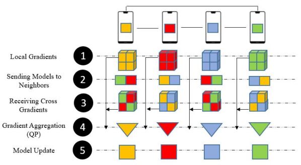
Figure 1: Algorithm overview. In the proposed CGA algorithm (1) each agent computes gradients of model parameters on its own data set; (2) each agent sends its model parameters to its neighbors; (3) each agent computes the gradients of its neighbors’ models on its own data set and sends the cross gradients back to the respective neighbors; (4) cross gradients and local gradients are projected into an aggregated gradient (using Quadratic Programming); which is then used to (5) update the model parameter.

Table 1: Comparison between different decentralized learning approaches. Rate: convergence rate for the optimization algorithm, Comm.: Communication overhead per mini-batch, Bo. Gr. Var.: Bounded gradient variances and variations as an assumption, Bo. Sec. Mom.: Bounded second moment of the gradient as an assumption, $m_{s}$: model size for the local agent, $N_{b}$: total number of non-zero elements in $\Pi$ (total number of communications per mini-batch), $\gamma$: auxiliary costs due to forward and backward pass of the neural network, $b$: floating point precision of arithmetic computations (e.g. 64)

Method	Rate	Comm.	Bo. Gr. Var.	Bo. Sec. Mom.
DPSGD	$\mathcal{O}(\frac{1}{K}+\frac{1}{\sqrt{NK}})$	$\mathcal{O}(m_{s}N_{b}+\gamma)$	Yes	No
SGP	$\mathcal{O}(\frac{1}{K}+\frac{1}{K^{1.5}}+\frac{1}{\sqrt{NK}})$	$\mathcal{O}(m_{s}N_{b}+\gamma)$	Yes	No
SwarmSGD	$\mathcal{O}(\frac{1}{\sqrt{K}})$	$\mathcal{O}(m_{s}\frac{N_{b}}{2}+\gamma)$	No	Yes
CGA (ours)	$\mathcal{O}(\frac{1}{K}+\frac{1}{K^{1.5}}+\frac{1}{\sqrt{NK}}+\frac{1}{K^{2}})$	$\mathcal{O}(2m_{s}N_{b}+\gamma)$	Yes	No

^∗ The communication overhead per mini-batch for CompCGA method is $\mathcal{O}(\frac{2m_{s}N_{b}}{b}+\gamma)$

Decentralized learning: While having a central parameter server is acceptable for data center applications, in certain use cases (such as learning over a wide-area distributed sensor network), continuous communication with a central parameter server is often not feasible (Haghighat et al., 2020). To address this concern, several decentralized learning algorithms have been proposed, where agents only interact with their neighbors without a central parameter server.

Recent advances in decentralized learning involve gossip averaging algorithms (Boyd et al., 2006; Xiao and Boyd, 2004; Kempe et al., 2003). Combining SGD with gossip averaging, Lian et al. (2017) shows analytically that decentralized parallel SGD (DPSGD) has far less communication overhead than its central counterpart (Dekel et al., 2012). Along the same line of work, Scaman et al. (2018) introduced a multi-step primal-dual algorithm while  Yu et al. (2019) and Balu et al. (2021) introduced the momentum version of DPSGD.  Tang et al. (2019) proposed DeepSqueeze, error-compensated compression is used in decentralized learning to achieve the same convergence rate as the one of centralized algorithms.  Koloskova et al. (2019) utilized compression strategies to propose CHOCO-SGD algorithm which learns from agents connected in varying topologies. Similarly with the aid of compression, Lu and De Sa (2020) and Vogels et al. (2020) introduced compression-based algorithms that improves the memory usage and running time of existing decentralized learning approaches. Assran et al. (2019) proposed the SGP algorithm which converges at the same sub-linear rate as SGD and achieves high accuracy on benchmark datasets. Additionally, Koloskova et al. (2020) presented a unifying framework for decentralized SGD analysis and provided the best convergence guarantees. More recently, SwarmSGD was proposed by Nadiradze et al. (2019) which leverages random interactions between participating agents in a graph to achieve consensus. In a recent work, Arjevani et al. (2020) proposes using AGD to achieve optimal convergence rate both in theory and practice. Jiang et al. (2018) propose multiple consensus and optimality rounds and the tradeoff between the consensus and optimality in decentralized learning.

Handling non-IID data: It is well known that decentralized learning algorithms can achieve comparable performance with its centralized counterpart under the so-called IID (independently and identically distributed) assumption. This refers to the situation where the training data is distributed in a uniformly random manner across all the agents. However, in real life applications, such an assumption is difficult to satisfy. Considering centralized learning literature, Li et al. (2018) proposed a variant of FL by adding a penalty term in the local objective function in FedProx algorithm. They further showed that their algorithm achieves higher accuracy when learning from non-IID data compared to FedAvg. Motivated by life-long learning (Shoham et al., 2019), FedCurv was proposed by adding a penalty term to the local loss function, with respect to Fisher information matrix. In another research study, FedAvg-EMD (Zhao et al., 2018) utilized the earth mover’s distance (EMD) as a metric to quantify the distance between the data distribution on each client and the population distribution, which was perceived as the root cause of problems arising in the non-IID scenario. Li et al. (2019b) showed the limitations with FedAvg on non-IID data analytically. Also, FedNova was proposed in which they use a normalized gradient in the update law of FedAvg after they show that the standard averaging of client models after heterogeneous local updates results in convergence to a stationary point (Wang et al., 2020). Similar to the case of decentralized learning, compression techniques (Sattler et al., 2019; Rothchild et al., 2020), momentum variant of algorithms (Wang et al., 2019; Li et al., 2019a), the use of adaptive gradients (Tong et al., 2020), and use of controllers in agent’s and server’s models (Karimireddy et al., 2019a) are also used in centralized learning for coping with non-IID data.  Hsieh et al. (2019) proposes a solution for learning from non-IID data by Estimating the degree of deviation from IID by moving the model from one data partition to another. They then Evaluate the accuracy on the other data set and calculate the accuracy loss, and based on this measure, SkewScout controls the communication tightness by automatically tuning the hyper-parameters of the decentralized learning algorithm. In their experimental results, they consider until $80\%$ non-IID data whereas in our approach our dataset is partitioned in a fully non-IID was based on the classes.

Although the above centralized approaches can handle departure from IID assumption, there still exists a gap in decentralized learning and several approaches fail under significant non-IID distribution of data among the agents (Hsieh et al., 2019; Jiang et al., 2017).

Contributions: To overcome the issue of handling non-IID data distributions in a decentralized learning setting, we propose the Cross-Gradient Aggregation (CGA) algorithm in this paper. We show its effectiveness in learning (deep) models in a decentralized manner from both IID and non-IID data distributions. Inspired by continual learning literature (Lopez-Paz and Ranzato, 2017), we devise an algorithm which in each step of training, collects the gradient information of each agent’s model on all its neighbors’ datasets and projects them into a single gradient which is then used to update the model. We use quadratic programming (QP) to obtain such a projected gradient. We provide an illustration of this algorithm in Figure 1.

The communication cost for our proposed algorithm is higher than the other state-of-the-art algorithms due to additional cost for two-way communication of the model parameters to, and the gradient information from, the neighbors. A comparison of the communication costs is provided in Table 1. Therefore, we also propose a compressed variant (CompCGA) to reduce the communication cost. Finally we validate the performance of our algorithms on MNIST and CIFAR-10 with different graph typologies. Our code is publicly available on GitHub. We then compare the effectiveness of our algorithm with SwarmSGD (Nadiradze et al., 2019), SGP (Assran et al., 2019), and DPSGD (Lian et al., 2017) and show that we can achieve higher accuracy in learning from non-IID data compared to the state-of-the-art decentralized learning approaches. Note that the goal here is to provide comparison between different decentralized learning algorithms; therefore, studies proposing novel compression schemes (Tang et al., 2019; Koloskova et al., 2019; Lu and De Sa, 2020; Vogels et al., 2020) are excluded from our comparison.

In summary, (i) we introduce the concept of cross gradients to develop a novel decentralized learning algorithm (CGA) that enables learning from both IID and non-IID data distributions, (ii) to reduce the higher communication costs of CGA, we propose a compressed variant, CompCGA that maintains a reasonably good performance in both IID and non-IID settings, (iii) we provide a detail convergence analysis of our proposed algorithm and show that we have similar convergence rates to the state-of-the-art decentralized learning approaches as summarized in Table 1, (iv) we demonstrate the efficacy of our proposed algorithms on benchmark datasets and compare performance with state-of-the-art decentralized learning approaches.

2 Cross-Gradient Aggregation

Let us first present a general problem formulation for decentralization deep learning, and then use it to motivate the Cross-Gradient Aggregation (CGA) algorithmic framework.

2.1 Problem Formulation

Very broadly, decentralized learning involves $N$ agents collaboratively solving the empirical risk minimization problem:

$$\textnormal{min}_{\mathbf{x}\in\mathbb{R}^{d}}\mathcal{F}(\mathbf{x}):=\frac{1}{N}\sum^{N}_{i=1}f_{i}(\mathbf{x}),$$ (1)

where $f_{i}(\mathbf{x}):=\mathbb{E}_{\zeta_{i}\sim\mathcal{D}_{i}}[F_{i}(\mathbf{x};\zeta_{i})]$ denotes a loss function defined in terms of dataset $\mathcal{D}_{i}$ that is private to agent $i\in[N]$. The agents are assumed to be communication-constrained and can only exchange information with their neighbors (where neighborliness is defined according to a weighted undirected graph with edge set $\mathbb{C}$ and adjacency matrix $\Pi$). Note that the adjacency matrix $\Pi$ is a doubly stochastic matrix constructed using the edge set of the graph, $\mathbb{C}$. For $(i,j)\notin\mathbb{C}$, we assign zero link weights (i.e., $\pi_{ij}=0$), and if $(i,j)\in\mathbb{C}$, the link weights are assigned such that the $\Pi$ is stochastic and symmetric, e.g., for a ring topology, $\pi_{ij}=\frac{1}{3}$ if $j\in\{i-1,i,i+1\}$. The goal is for the agents to come up with a consensus set of model parameters $\mathbf{x}$ (although during training each agent operates on its own copy of $\mathbf{x}$.)

Usual approaches in decentralized learning involve each agent alternating between updating the local copies of their parameters using gradient information from their private datasets, and exchanging parameters with its neighbors. We depart from this usual path by first introducing two key concepts.

Definition 1.

For agent $j$, consider the dataset $\mathcal{D}_{j}$, the differentiable objective function $f_{j}$, and the model parameter copy $\mathbf{x}^{j}$. The self-gradient is defined as:

$$\mathbf{g}^{jj}:=\nabla_{\mathbf{x}}f_{j}(\mathcal{D}_{j};\mathbf{x}^{j})\,.$$ (2)

Definition 2.

For a pair of agents $j,l$, consider the dataset $\mathcal{D}_{l}$, the differentiable objective function $f_{l}$, and the model parameter copy $\mathbf{x}^{j}$. The cross-gradient is defined as:

$$\mathbf{g}^{jl}:=\nabla_{\mathbf{x}}f_{l}(\mathcal{D}_{l};\mathbf{x}^{j})\,.$$ (3)

In words, the cross-gradient is calculated by evaluating the gradient of the loss function private to agent $l$ at the parameters of agent $j$. Both the self-gradient $\mathbf{g}^{jj}$ and the cross-gradient $\mathbf{g}^{jl}$ immediately lend themselves to their stochastic counterparts (implemented by simply mini-batching the private datasets); in the rest of the paper, we will operate under this setting.

2.2 The CGA Algorithm

We now propose the CGA algorithm for decentralized deep learning. Figure 1 provides a visual overview of the method. Recall that $\mathbf{x}^{j}$ is the model parameter copy for each agent $j$ which is initialized by training with $\mathcal{D}_{j}$. Pick the number of iterations $K$, step-size $\alpha$, and the momentum coefficient $\beta$ as user-defined inputs.

In the $k^{\textrm{th}}$ iteration of CGA, each agent $j\in[N]$ calculates its self-gradient $\mathbf{g}_{k}^{jj}$. Then, agent $j$’s model parameters are transmitted to all other agents ($l$) in its neighborhood, and the respective cross-gradients are calculated and transmitted back to agent $j$ and stacked up in a matrix $\mathbf{G}_{k}^{j}$. Then $\mathbf{G}_{k}^{j}$ and $\mathbf{g}_{k}^{jj}$ are used to perform a quadratic programming (QP) projection step, which we discuss in detail below. To accelerate convergence, a momentum-like adjustment term is also incorporated to obtain the final update law.

Algorithm 1 Cross-Gradient Aggregation (CGA)

Initialize: $\mathcal{D}_{j},\mathbf{x}_{0}^{j},\mathbf{v}_{0}^{j},(j=1,2,\dots,N),\alpha,\beta,K$, a QP solver
for $k=1:K$ do

       for $j=1:N$ do

             Randomly shuffle the data subset $\mathcal{D}_{j}$
Compute $\mathbf{g}_{k}^{jj}$
$\mathbf{G}^{j}=\{\}$
for each agent $l$ s.t. $(j,l)\in\mathbb{C}$ do

                   Compute $\mathbf{g}_{k}^{jl}$
$\mathbf{G}_{k}^{j}\leftarrow\mathbf{G}_{k}^{j}\cup\mathbf{g}_{k}^{jl}$

             end for

            $\mathbf{w}_{k}^{j}=\sum_{l}\mathbf{\pi}_{jl}\mathbf{x}_{k-1}^{l}$
$\tilde{\mathbf{g}}_{k}^{j}\leftarrow\texttt{QP}(\mathbf{g}_{k}^{jj},\mathbf{G}_{k}^{j})\;\;\;$
$\mathbf{v}^{j}_{k}=\beta\mathbf{v}^{j}_{k-1}-\alpha\tilde{\mathbf{g}}_{k}^{j}$
$\mathbf{x}^{j}_{k}=\mathbf{w}_{k}^{j}+\mathbf{v}^{j}_{k}$

       end for

      

end for

The form of the algorithm is similar to momentum-accelerated consensus SGD (Jiang et al., 2017). The key difference in Algorithm 1 when compared to existing gradient-based learning methods is the QP projection step. We observe that the local gradient $\tilde{\mathbf{g}}^{j}$ is obtained via a nonlinear projection, instead of just the self-gradient $\mathbf{g}^{jj}$ (as is done in standard momentum-SGD), or a linear averaging of self-gradients in the neighborhood $\mathbb{C}$ (as is done in standard decentralized learning methods).

The motivation for this difference stems from the nature of the cross-gradients $\mathbf{g}_{k}^{jl}$. In the IID case, these should statistically resemble the self-gradient $\mathbf{g}_{k}^{jj}$, and hence standard momentum averaging would succeed. However, with non-IID data partitioning, the differences between the cross-gradients in different agents becomes so significant and consensus may be difficult to achieve, leading to overall poor convergence properties. Therefore, in the non-IID case we need an alternative approach.

We leverage the following intuition, borrowed from (Lopez-Paz and Ranzato, 2017). We seek a descent direction that is close to $\mathbf{g}_{k}^{ll}$ and simultaneously is positively correlated with all the cross-gradients. This can be modeled via a QP projection, posed in primal form as follows:

$$\text{min}_{\mathbf{z}}\;\frac{1}{2}\mathbf{z}^{\top}\mathbf{z}-\mathbf{g}^{\top}\mathbf{z}+\frac{1}{2}\mathbf{g}^{\top}\mathbf{g}$$ (4a)

$$\text{s.t.~{}}\;\mathbf{G}\mathbf{z}\geq 0$$

where $\mathbf{g}:=\mathbf{g}_{k}^{jj}$ and $\mathbf{G}:=(\mathbf{g}^{jl})\;\;\forall(j,l)\in\mathbb{C}$. The dual formulation of the above QP can be posed as:

$$\text{min}_{\mathbf{u}}\;\frac{1}{2}\mathbf{u}^{\top}\mathbf{G}\mathbf{G}^{\top}\mathbf{u}+\mathbf{g}^{\top}\mathbf{G}^{\top}\mathbf{u}$$ (5a)

$$\text{s.t.~{}}\;\mathbf{u}\geq 0$$

which is more efficient from a computational standpoint. Once we solve for the optimal dual variable $\mathbf{u}^{*}$, we can recover the optimal projection direction $\mathbf{g}^{*}$ using the relation $\mathbf{g}^{*}=\mathbf{G}^{\top}\mathbf{u}^{*}+\mathbf{g}$.

2.3 The Compressed CGA Algorithm

The CGA algorithm requires multiple exchanges of model parameters and gradients between neighbor agents in each iteration, which can be a burden particularly in communication-constrained environments. To reduce the communication bandwidth, we propose adding a compression layer on top of the CGA framework. For that purpose, we use Error Feedback SGD (EF-SGD) (Karimireddy et al., 2019b) to compress gradients. The resulting algorithm is same as Algorithm 1; except that instead of regular self- and cross-gradients, a scaled signed gradient is calculated, the error between the compressed and non-compressed gradients will be computed ($e^{ij}_{k}$ in the algorithm), and this error will be added as a penalty term to the gradients in the next step. The resulting algorithm is shown in Algorithm 2. In the pseudo code provided there, the quantity $d$ corresponds to the dimension of the computed gradients for each agent.

Algorithm 2 Compressed Cross-Gradient Aggregation (CompCGA)

Initialize: $\mathcal{D}_{j},\mathbf{e}_{0}^{j},\mathbf{x}_{0}^{j},\mathbf{v}_{0}^{j},(j=1,\dots,N),\alpha,\beta,K$, a QP solver
for $k=1:K$ do

       for $j=1:N$ do

             Randomly shuffle the data subset $\mathcal{D}_{j}$
Compute $\mathbf{g}_{k}^{jj}$
$\mathbf{p}_{k}^{jj}=\mathbf{g}_{k}^{jj}+\mathbf{e}_{k}^{jj}$
$\mathbf{\delta}_{k}^{jj}=(\|\mathbf{p}_{k}^{jj}\|_{1}/d)sgn(\mathbf{p}_{k}^{jj})$
$\mathbf{G}^{j}=\{\}$
for each agent $l$, s.t. $(j,l)\in\mathbb{C}$ do

                   Compute $\mathbf{g}_{k}^{jl}$
$\mathbf{p}_{k}^{jl}=\mathbf{g}_{k}^{jl}+\mathbf{e}_{k}^{jl}$
$\mathbf{\delta}_{k}^{jl}=(\|\mathbf{p}_{k}^{jl}\|_{1}/d)sgn(\mathbf{p}_{k}^{jl})$
$\mathbf{e}^{jl}_{k}=\mathbf{p}^{jl}_{k}-\mathbf{\delta}_{k}^{jl}$
$\mathbf{G}^{j}\leftarrow\mathbf{G}^{j}\cup\mathbf{\delta}_{k}^{jl}$

             end for

            $\mathbf{w}_{k}^{j}=\sum_{l}\mathbf{\pi}_{jl}\mathbf{x}_{k-1}^{l}$
$\tilde{\mathbf{g}}^{j}\leftarrow\texttt{QP}(\mathbf{\delta}_{k}^{jj},\mathbf{G}^{j})\;\;\;$
$\mathbf{v}^{j}_{k}=\beta\mathbf{v}^{j}_{k-1}-\alpha\tilde{\mathbf{g}}^{j}$
$\mathbf{x}^{j}_{k}=\mathbf{w}_{k}^{j}+\mathbf{v}^{j}_{k}$
$\mathbf{e}^{jj}_{k}=\mathbf{p}^{jj}_{k}-\mathbf{\delta}_{k}^{jj}$

       end for

      

end for

3 Convergence Analysis for CGA

We now present a theoretical analysis of our proposed CGA approach. It should be noted that the communication among the agents is assumed to be synchronous in the following analysis. Let us begin with a definition of smoothness.

Definition 3.

A function $\mathcal{F}(\cdot)$ is $L$-smooth if $\forall\mathbf{x},\mathbf{y}$:

$$\mathcal{F}(\mathbf{x})\leq\mathcal{F}(\mathbf{y})+\nabla\mathcal{F}(\mathbf{y})^{\top}(\mathbf{x}-\mathbf{y})+\frac{L}{2}\|\mathbf{x}-\mathbf{y}\|^{2}.$$ (6)

In order to analyze the convergence of decentralized learning algorithms, the following assumptions are standard.

Assumption 1.

Each function $f_{i}(\mathbf{x})$ is $L$-smooth.

Assumption 2.

There exist $\sigma>0$ and $\delta>0$ such that

$$\mathbb{E}_{\zeta\sim\mathcal{D}_{i}}[\|\nabla F_{i}(\mathbf{x};\zeta)-\nabla f_{i}(\mathbf{x})\|]\leq\sigma^{2},$$ (7)

and that

$$\frac{1}{N}\sum_{i=1}^{N}\|\nabla f_{i}(\mathbf{x})-\nabla\mathcal{F}(\mathbf{x})\|^{2}\leq\delta^{2}.$$ (8)

Assumption 3.

Define $\mathbf{g}^{i}=\nabla F_{i}(\mathbf{x};\zeta)$. Then, there exists $\epsilon>0$ such that

$$\mathbb{E}_{\zeta\sim\mathcal{D}_{i}}[\|\tilde{\mathbf{g}}^{i}-\mathbf{g}^{i}\|^{2}]\leq\epsilon^{2}.$$ (9)

Assumption 1 implies that $\mathcal{F}(\mathbf{x})$ is $L$-smooth. Assumption 2 assumes bounded variances due to non-IID-ness. Equation 7 bounds the variance within the same agent ("intra-variance") while Equation 8 bounds the variance among different agents ("inter-variance").

Assumption 3 is necessitated by our adoption of the QP projection step. Intuitively, if the local optimization problem is meaningful, then this assumption holds. In this assumption, the value of $\epsilon$ is governed by the difference between the data distributions possessed by each agent. Note that thus far, Eq. 8 has been used to study the effect of non-IID data in most analyses of decentralized learning; previous methods operate upon $\mathbf{g}^{i}$. In our work, we combine both Eq. 8 and Eq. 9 to mathematically show convergence.

We next impose another assumption on the graph that serves to characterize consensus.

Assumption 4.

The mixing matrix $\mathbf{\Pi}\in\mathbb{R}^{N\times N}$ is a doubly stochastic matrix with $\lambda_{1}(\mathbf{\Pi})=1$ and

$$\text{max}\{|\lambda_{2}(\mathbf{\Pi})|,|\lambda_{N}(\mathbf{\Pi})|\}\leq\sqrt{\rho}<1,$$ (10)

where $\lambda_{i}(\mathbf{\Pi})$ is the $i$th-largest eigenvalue of $\mathbf{\Pi}$ and $\rho$ is a constant.

3.1 Theoretical Results

We now present our theoretical characterization of CGA. We focus only on the case of non-convex objective functions. All detailed proofs are presented in the Appendix, and follow from basic algebra and sequence convergence theory. Below, $i$ indicates the agent index; the average of all agent model copies is represented by $\bar{\mathbf{x}}$; throughout the analysis, we assume that the objective function value is bounded below by $\mathcal{F}^{*}$. We also denote $a_{n}=\mathcal{O}(b_{n})$ if $a_{n}\leq c\>b_{n}$ for some constant $c>0$.

We first present a lemma showing that CGA achieves consensus among the different agents, and then prove our main theorem indicating convergence of the algorithm.

Lemma 1.

Let Assumptions 1-4 hold. Define $\{\bar{\mathbf{x}}_{k}\},\forall k\geq 0$ as the agent average sequence obtained by the iterations of CGA. If $\beta\in[0,1)$ is the momentum coefficient, then for all $K\geq 1$, we have:

$$\begin{split}&\sum_{k=0}^{K-1}\frac{1}{N}\sum_{i=1}^{N}\mathbb{E}\bigg{[}\bigg{\|}\bar{\mathbf{x}}_{k}-\mathbf{x}^{i}_{k}\bigg{\|}^{2}\bigg{]}\leq\\ &\frac{2\alpha^{2}}{(1-\beta)^{2}}\bigg{(}\frac{\epsilon^{2}}{1-\rho}+\frac{3\sigma^{2}}{(1-\sqrt{\rho})^{2}}+\frac{3\delta^{2}}{(1-\sqrt{\rho})^{2}}\bigg{)}K+\\ &\frac{6\alpha^{2}}{(1-\beta)^{2}(1-\sqrt{\rho})}\sum_{k=0}^{K-1}\mathbb{E}[\|\frac{1}{N}\sum_{i=1}^{N}\nabla f_{i}(\mathbf{x}^{i}_{k})\|^{2}].\end{split}$$ (11)

A complete proof can be found in the Supplementary Section A.1. From Lemma 1, we can observe that the evolution of the deviation of the model copies from their average can be attributed to two terms. The first is the following constant:

$$\frac{2\alpha^{2}}{(1-\beta)^{2}}\bigg{(}\underbrace{\frac{\epsilon^{2}}{1-\rho}}_{I}+\underbrace{\frac{3\sigma^{2}}{(1-\sqrt{\rho})^{2}}}_{II}+\underbrace{\frac{3\delta^{2}}{(1-\sqrt{\rho})^{2}}}_{III}\bigg{)}K,$$

where (I) is controlled by Assumption 3 (which also implies how well the local QP is solved), (II) is related to sampling variance, and (III) indicates the gradient variations (determined by the data distributions). Additionally, the step size and momentum coefficient can be tuned to reduce the negative impact of these variance coefficients. The second is the following term:

$$\frac{6\alpha^{2}}{(1-\beta)^{2}(1-\sqrt{\rho})}\underbrace{\sum_{k=0}^{K-1}\mathbb{E}[\|\frac{1}{N}\sum_{i=1}^{N}\nabla f_{i}(\mathbf{x}^{i}_{k})\|^{2}]}_{IV},$$

where (IV) is the summation of the squared norms of average gradients, the effect of which can be controlled by leveraging the step size and momentum coefficient.

Lemma 1 also aligns with the well-known result phenomenon in decentralized learning that the consensus error is inversely proportional to the spectral gap of the graph mixing matrix. Using the above lemma, we obtain the following main result.

Theorem 1.

Let Assumptions 1-4 hold. Suppose that the step size $\alpha$ satisfies the following relationships:

$$\begin{cases}0<\alpha\leq\frac{\beta L}{(1-\beta)^{2}}\\ 1-\frac{6\alpha^{2}L^{2}}{(1-\beta)(1-\sqrt{\rho})^{2}}-\frac{4L\alpha}{(1-\beta)^{2}}\geq 0.\end{cases}$$ (12)

For all $K\geq 1$, we have

$$\begin{split}&\frac{1}{K}\sum_{k=0}^{K-1}\mathbb{E}\left[\left\|\nabla\mathcal{F}\left(\bar{\mathbf{x}}_{k}\right)\right\|^{2}\right]\leq\\ &\frac{1}{C_{1}K}\left(\mathcal{F}\left(\bar{\mathbf{x}}_{0}\right)-\mathcal{F}^{*}\right)+\bigg{(}2C_{2}+C_{3}\frac{\alpha^{2}\beta}{(1-\beta)^{4}}+C_{4}+\\ &C_{5}\frac{2\alpha^{2}}{(1-\beta)^{2}(1-\rho)}\bigg{)}\epsilon^{2}+\bigg{(}\frac{2}{N}(C_{2}+C_{3}\frac{\alpha^{2}\beta}{(1-\beta)^{4}})+\\ &C_{5}\frac{6\alpha^{2}}{(1-\beta)^{2}(1-\sqrt{p})^{2}}\bigg{)}\sigma^{2}+C_{5}\frac{6\alpha^{2}}{(1-\beta)^{2}(1-\sqrt{\rho})^{2}}\delta^{2},\\ \end{split}$$ (13)

where $C_{1}=\frac{\alpha}{2(1-\beta)}-\frac{(1-\beta)\alpha^{2}}{2\beta L}$, $C_{2}=\left(\frac{\beta L\alpha^{2}}{2(1-\beta)^{3}}+\frac{\alpha^{2}L}{(1-\beta)^{2}}\right)/C_{1}$, $C_{3}=\frac{(1-\beta)L}{2\beta}/C_{1}$,

$C_{4}=\frac{\beta L}{2(1-\beta)^{3}}/C_{1}$, $C_{5}=\frac{\alpha L^{2}}{2(1-\beta)}/C_{1}$.

A complete proof of Theorem 1 is discussed in the Supplementary Section A.2.

Theorem 1 shows that the average gradient magnitude achieved by the consensus estimates is upper-bounded by the difference between initial objective function value and the optimal value, as well as how well the local QP is solved, the sampling variance, and the non-IID-ness. The coefficients before these constants are determined by $\alpha$, $\beta$, and $L$; judicious selection of $\alpha$ and $\beta$ can be performed to reduce the error bound. Additionally, the step size is required to satisfy two conditions as listed in the above theorem statement. The second condition can be solved to get another upper bound, denoted by $\alpha^{*}$ (which will be shown in the Appendix section). Hence, if we choose $0<\alpha\leq\text{min}\{\frac{\beta L}{(1-\beta)^{2}},\alpha^{*}\}$, the last inequality naturally holds. We next present a corollary to explicitly show the convergence rate of CGA.

Corollary 1.

Suppose that the step size satisfies $\alpha=\mathcal{O}(\frac{\sqrt{N}}{\sqrt{K}})$ and that $\epsilon=\mathcal{O}(\frac{1}{\sqrt{K}})$. For a sufficiently large $K\geq\textnormal{max}\{\frac{144NL^{2}}{r^{2}},\frac{N}{\beta^{2}L^{2}}\},r=(1-\sqrt{\rho})\sqrt{16(1-\sqrt{\rho})^{2}+24(1-\beta)^{3}}-4(1-\sqrt{\rho})^{2}$, we have, for some constant C > 0,

$$\frac{1}{K}\sum_{k=0}^{K-1}\mathbb{E} \left[\left\|\nabla\mathcal{F}\left(\bar{\mathbf{x}}_{k}\right)\right\|^{2}\right]$$

$$\leq C\Bigg{(}\frac{1}{\sqrt{NK}}+\frac{1}{K}+\frac{1}{K^{1.5}}+\frac{1}{K^{2}}\Bigg{)}.$$ (14)

An immediate observation is that when $K$ is sufficiently large, the term $\mathcal{O}(\frac{1}{\sqrt{NK}})$ will dominate the convergence rate such that the linear speed up can be achieved, if increasing the number of agents $N$. This convergence rate matches the well-known best result in decentralized SGD algorithms in literature.

Analysis of CompCGA. We now provide some qualitative arguments to facilitate the understanding of CompCGA. Though we have not directly established its convergence rates, we can presumably extend the analysis of CGA to this setting. Observe that the core update laws for $\mathbf{x}$ are the same for CompCGA as in CGA, but equipped with gradient compression. Moreover, for our theoretical analysis presented for CGA, the specific way in which $\tilde{\mathbf{g}}$ is calculated does not play a role, and additional compression can perhaps be modeled by changing the variation constants. Therefore, we hypothesize that CompCGA also exhibits a convergence rate of $\mathcal{O}(\frac{1}{\sqrt{NK}})$. This is also evidently seen from our empirical studies, which we present next.

4 Experimental Results

In this section, we analyze the performance of CGA algorithm empirically. We compare the effectiveness of our algorithms with other baseline decentralized algorithms such as SwarmSGD (Nadiradze et al., 2019), SGP (Assran et al., 2019), and the momentum variant of DPSGD (Lian et al., 2017) (DPMSGD).

Setup. We present the empirical studies on CIFAR-10 and MNIST datasets (MNIST results can be found in the Supplementary Section A.6). To explore the algorithm performance under different situations, the experiments are performed with $5$, $10$ , and $40$ agents. Here, we consider an extreme form of non-IID-ness by assigning different classes of data to each agent. For example, when there are $5$ agents, each agent has the data for $2$ distinct classes, and similarly when there are $10$ agents, each agent has the data for $1$ distinct class. When the number of agents are more than the number of classes, each class is divided into a sufficient number of subsets of samples and agents are randomly assigned distinct subsets. We use a deep convolutional neural network (CNN) model (with 2 convolutional layers with $32$ filters each followed by a max pooling layer, then $2$ more convolutional layers with $64$ filters each followed by another max pooling layer and a dense layer with 512 units, ReLU activation is used in convolutional layers) for our validation experiments. Additionally, We use a VGG11 (Simonyan and Zisserman, 2014) model for CIFAR-10 (Detailed CIFAR-10 results can be found in the Supplementary Section A.5). A mini-batch size of $128$ is used, the initial step-size is set to $0.01$ for CIFAR-10, and step size is decayed with constant $0.981$. The stopping criterion is a fixed number of epochs and the momentum parameter ($\beta$) is set to be 0.98. The consensus model is then used to be evaluated on the local test sets and the average accuracy is reported.

The experiments are performed on a large high-performance computing cluster with a total of 192 GPUs distributed over 24 nodes. Each node in the cluster is made of 2 Intel Xeon Gold 6248 CPUs with each 20 cores and 8 Tesla V100 32GB SXM2 GPUs. An experiment with 40 agents on a VGG11 model for CIFAR10 dataset takes about $55$ seconds per epoch for execution. The code for performing the experiments is publicly available.

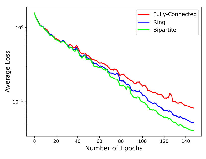
(a)

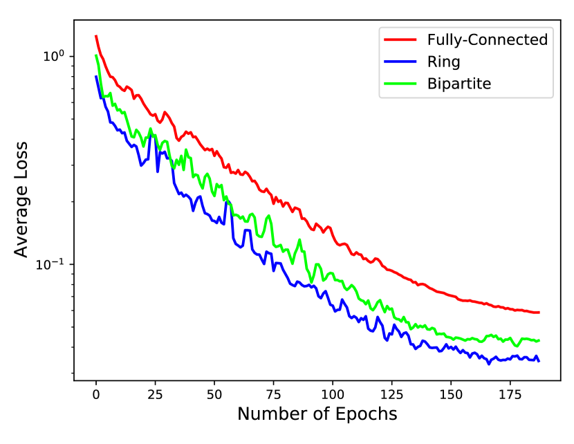
(b)

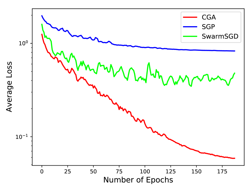
(c)

Figure 2: Average training loss (log scale) for (a) CGA method on IID (b) CGA method on non-IID data distributions (c) different methods on non-IID data distributions for training 5 agents using CNN model architecture

4.1 CGA convergence characteristics

We start by analyzing the performance of CGA algorithm on CIFAR-10. Figure 2 shows the convergence characteristics of our proposed algorithm via training loss versus epochs. Figure 2(a) shows the convergence characteristics of CGA for IID data distributions for different communication graph topologies. While the fully connected graph represents a dense topology, the ring and bipartite graphs represent relatively much sparser topologies.

We observe that the convergence behavior induced by the training loss remain similar across the different graph topologies, though at the final stage of training, the ring and bipartite networks moderately outperform the fully connected one. This can be attributed to more communication occurring for the fully connected case. The phenomenon of faster convergence with sparser graph topology is an observation that have been made by earlier research works in Federated Learning (McMahan et al., 2017) by reducing the client fraction which makes the mixing matrix sparser and decentralized learning (Jiang et al., 2017). However, as Figure 6(a) in the Supplementary Section A.5 shows, we observe that by training for more number of epochs, training losses associated with all graph topologies converge to similar values.

Figure 2(b) shows similar curves but for the non-IID case. In this case, we do observe a slight difference in convergence with faster rates for sparser topologies compared to their dense (fully connected) counterpart. Another phenomenon observed here is that for sparser topologies, the training process has more gradient variances and variations, which has been caused by the non-IID data distributions. This well matches the theoretical analysis we have obtained.

Finally, Figure 2(c) shows the comparison of convergence characteristics with other state-of-the-art decentralized algorithms with non-IID data distributions. CGA training is seen to be smoother compared to SwarmSGD, and to converge significantly faster compared to both SwarmSGD and SGP. From the theoretical analysis, we have shown that CGA enables to converge faster at the beginning although after a sufficiently large number of epochs, all methods listed here achieve the same rate $\mathcal{O}(\frac{1}{\sqrt{NK}})$.

Additionally, the SwarmSGD requires a geometrically distributed random variable to determine the number of local stochastic gradient steps performed by each agent upon interaction. That causes the largest variance shown in the loss curve in Figure 2(c). Note that since DPMSGD diverges for most of the non-IID experiments (see Table 3), we do not provide its loss plots here.

Table 2: Testing accuracy comparison for CIFAR10 with IID data distribution using CNN model architecture

Model	Fully-connected	Ring	Bipartite
DPMSGD	68.8% (5) 68.1% (10) 67.6% (40)	67.7% (5) 67.7% (10) 66.8% (40)	67.7% (5) 67.3% (10) 57.1% (40)
SGP	66.6% (5) 59.3% (10) 46.3% (40)	66.3% (5) 59.2% (10) 46.2% (40)	66.3% (5) 58.4% (10) 46.3% (40)
SwarmSGD	70.6% (5) 68.3% (10) 31.5% (40)	70.7% (5) 65.4% (10) 31.4% (40)	70.7% (5) 60.3% (10) 33.4% (40)
CGA (ours)	68.5 % (5) 68.5% (10) 64.6% (40)	67.9 % (5) 67.8% (10) 63.7% (40)	68.2 % (5) 68.2% (10) 58.4% (40)
CompCGA (ours)	68.4% (5) 62.2% (10) 63.3% (40)	68.3% (5) 62.9% (10) 53.4% (40)	68.4% (5) 64.6% (10) 56.6% (40)

Table 3: Testing accuracy comparison for CIFAR10 with non-IID data distribution using CNN model architecture

Model	Fully-connected	Ring	Bipartite
DPMSGD	Diverges (5) 10.1% (10) 10.5% (40)	Diverges (5) Diverges (10) 10.0% (40)	Diverges (5) 10.0% (10) 10.7% (40)
SGP	66.4% (5) 59.3% (10) 46.2% (40)	46.3% (5) 25.8% (10) 31.4% (40)	49.8% (5) 24.9% (10) 11.8% (40)
SwarmSGD	67.3% (5) 47.3% (10) 30.6% (40)	62.5% (5) 38.5% (10) 25.8% (40)	63.9% (5) 33.8% (10) 23.5% (40)
CGA (ours)	68.4% (5) 68.2% (10) 62.1% (40)	66.5% (5) 48.8% (10) 40.9% (40)	67.2% (5) 38.9% (10) 25.7% (40)
CompCGA (ours)	61.7% (5) 60.2% (10) 59.8% (40)	50.3% (5) 39.5% (10) 32.7% (40)	40.4% (5) 36.7% (10) 23.6% (40)

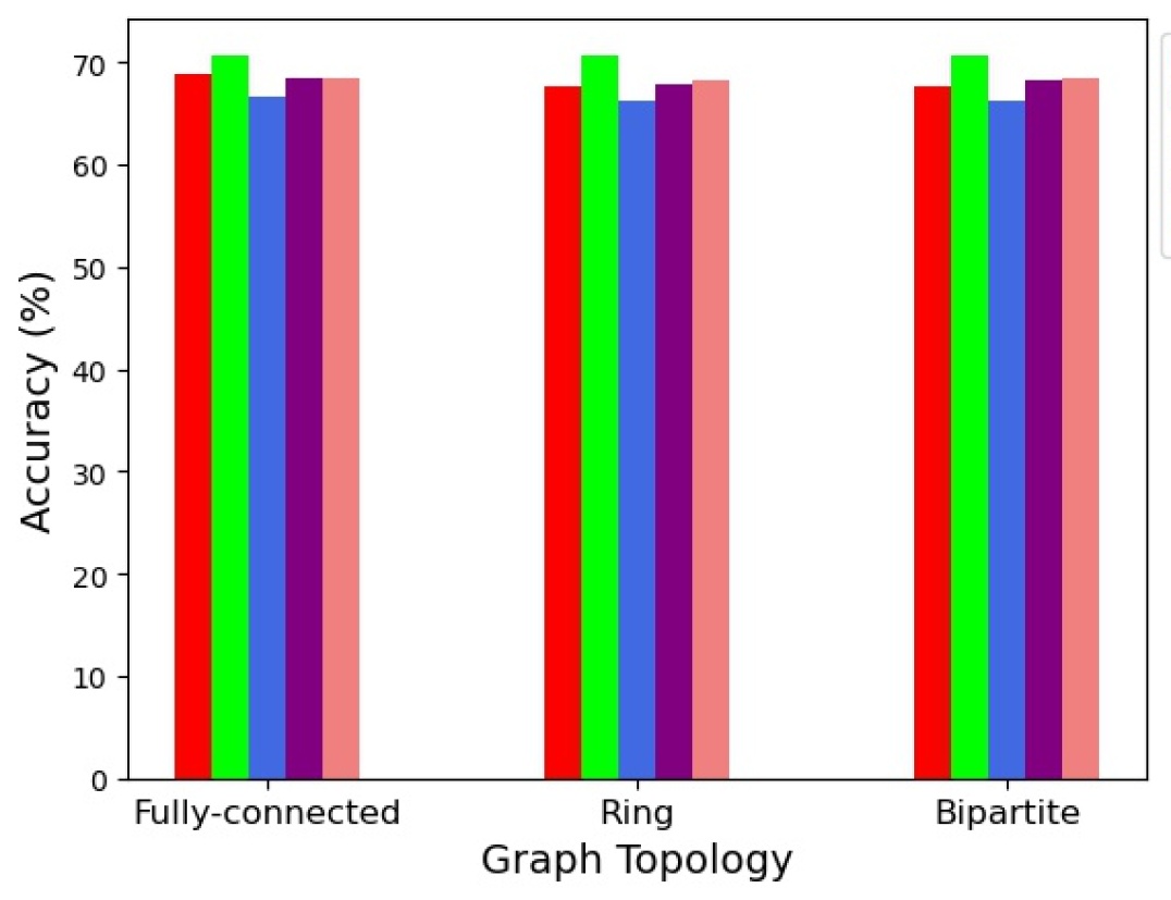
(a)

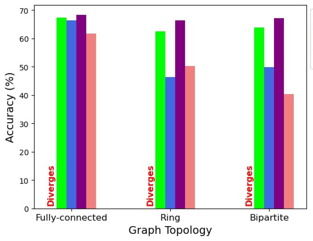
(b)

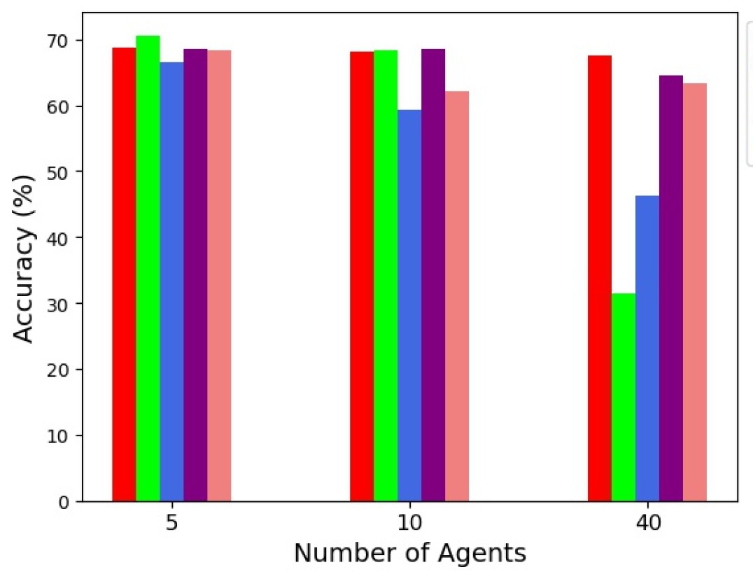
(c)

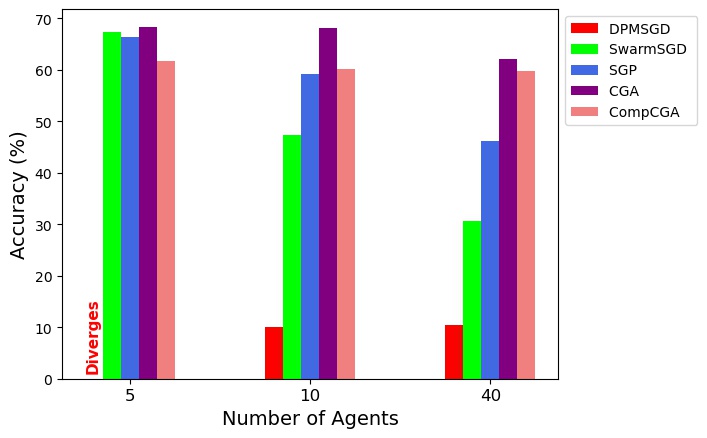
(d)

Figure 3: Average testing accuracy for different methods learning from (a) IID data distributions w.r.t graph topology (b) non-IID data distributions w.r.t graph topology (c) IID data distributions w.r.t the number of learning agents (d) non-IID data distributions w.r.t the number of learning agents

4.2 Comparative evaluation

We compare our proposed algorithm, CGA and its compressed version, compCGA with other state-of-the-art decentralized methods - DPMSGD, SGP and SwarmSGD. Note that in order to provide a fair comparison between the algorithms, there are some minor adjustments that we made during the experiments. For SGP optimizer, we considered the graph to be undirected where the connected agents could both send and receive information to and from each other. On top of that, the adjacency matrix $\mathbf{\Pi}$ in our experiments (a.k.a mixing matrix $P^{(k)}$ in Assran et al. (2019)) is fixed throughout the training process. In the implementation of SwarmSGD, we defined the number of local SGD steps, $H=1$, where the selected pair of agents perform only a single local SGD update before averaging their model parameters. In term of graph topologies, SwarmSGD was run not only on $r$-regular graphs (fully connected and ring) as described in Nadiradze et al. (2019), we also performed experiments using bipartite graph topology which is not $r$-regular.

As a baseline, we first provide a comparative evaluation for IID data distributions in Table 2. Results show that CGA performance is comparable with or slightly better than other methods in most cases with smaller number of agents, i.e., $5$ and $10$. However, we do observe a noticeable reduction in testing accuracy for SGP and SwarmSGD with $40$ agents communicating over Ring or Bipartite graphs (which is an expected trend as reported in Assran et al. (2019) and Sattler et al. (2019)). While the testing accuracy of CGA also decreases in these scenarios, the performance reduction is not as drastic in comparison. The performance of compCGA deteriorates slightly compared to CGA, while still maintaining better accuracy than other methods in most scenarios.

The advantage of CGA is much more pronounced under non-IID data distributions as seen in Table 3. With extreme non-IID data distributions, CGA achieves the highest accuracy for all scenarios with different number of learning agents and communication graph topologies. In contrast, the baseline method DPMSGD struggles significantly in all scenarios with non-IID data. Other methods (SGP and SwarmSGD) while having similar performance as CGA for $5$ agents and fully connected topology, their performances drop significantly more than that of CGA with higher number of agents and sparser communication graphs. CompCGA performs slightly worse than CGA, while still maintaining better accuracy than other methods in most scenarios.

Finally, we graphically summarize the overall trends that we observed in Figure 3. From Figure 3 (a) and (b), it is clear that while there is no appreciable impact of graph topology on testing accuracy under IID data distributions, the impact is quite significant under non-IID data distributions. The results shown here are with $5$ agents (see Supplementary Section A.5 for $10$ and $40$ agents). In this case, testing accuracy decreases for sparse graph topologies which conforms with observations made in Sattler et al. (2019). Figure 3 (c) and (d) show accuracy trends with respect to the number of agents. All results shown here are with fully connected topology (see Supplementary Section A.5 for other topologies). In this regard, Assran et al. (2019) shows a slight reduction in accuracy when the number of nodes/agents increase for both SGP and DPSGD methods. We see a similar trend here for both IID and non-IID data distributions. Clearly, the impact is more pronounced for non-IID data. However, the performance decrease with increase in number agents remain small for both CGA and CompCGA under non-IID data distributions. Also, as discussed in Table 1, we notice that the communication rounds for CGA is twice as that of SGP and 4 times the communication round of SwarmSGD. Therefore, we looked at their convergence properties w.r.t communication rounds. As Figure 4 shows, CGA converges to a lower loss value after $200$ communication rounds.

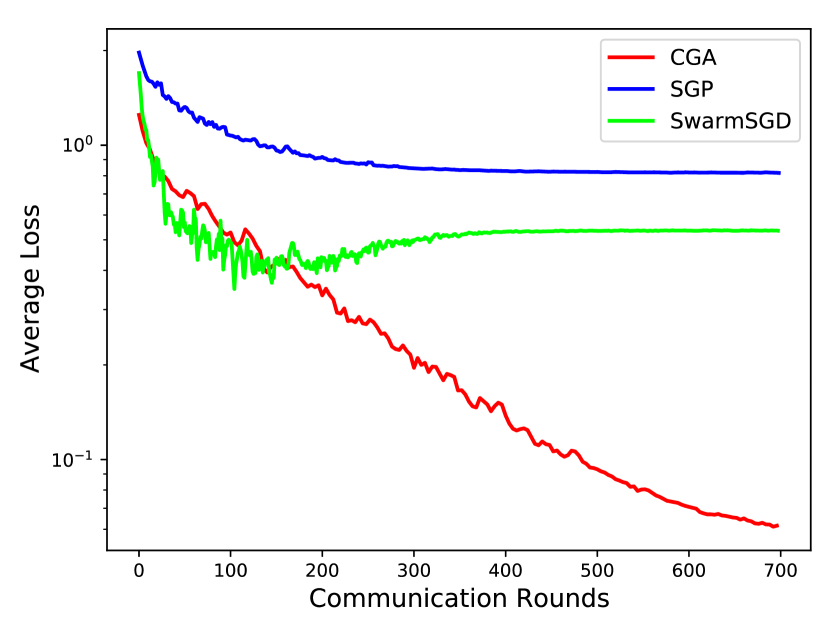
Figure 4: Average training loss (log scale) for different algorithms w.r.t communication rounds on non-IID data distributions (for 5 agents using CNN model architecture)

5 Conclusions

In this paper, we propose the Cross-Gradient Aggregation (CGA) algorithm to effectively learn from non-IID data distributions in a decentralized manner. We present convergence analysis for our proposed algorithm and show that we match the best known convergence rate for decentralized algorithms using CGA. To reduce the communication overhead associated with CGA, we propose a compressed variant of our algorithm (CompCGA) and show its efficacy. Finally, we compare the performance of both CGA and CompCGA with state-of-the-art decentralized learning algorithms and show superior performance of our algorithms especially for the non-IID data distributions. Future research will focus on addressing performance reduction in scenarios with a large number of agents communicating over sparse graph topologies.

6 Acknowledgements

This work was partly supported by the National Science Foundation under grants CAREER-1845969 and CAREER CCF-2005804. We would also like to thank NVIDIA^® for providing GPUs used for testing the algorithms developed during this research. This work also used the Extreme Science and Engineering Discovery Environment (XSEDE), which is supported by NSF grant ACI-1548562 and the Bridges system supported by NSF grant ACI-1445606, at the Pittsburgh Supercomputing Center (PSC).

Appendix A Appendix

A.1 Proof of Lemma 1

This section presents the detailed proof for Lemma 1. To begin with, we provide some technical auxiliary lemmas and the associated proof. We start with bounding the ensemble average of local optimal gradients.

The core update law for CGA is:

Lemma 2.

Let all assumptions hold. Let $g^{i}$ be the unbiased estimate of $\nabla f_{i}(\mathbf{x}^{i})$ at the point $\mathbf{x}^{i}$ such that $\mathbb{E}[\mathbf{g}^{i}]=\nabla f_{i}(\mathbf{x}^{i})$, for all $i\in[N]:=\{1,2,...,N\}$. Thus the following relationship holds

$$\mathbb{E}\bigg{[}\bigg{\|}\frac{1}{N}\sum_{i=1}^{N}\tilde{\mathbf{g}}^{i}\bigg{\|}^{2}\bigg{]}\leq\frac{2\sigma^{2}}{N}+2\mathbb{E}\bigg{[}\bigg{\|}\frac{1}{N}\sum_{i=1}^{N}\nabla f_{i}(\mathbf{x}^{i})\bigg{\|}^{2}\bigg{]}+2\epsilon^{2}.$$ (15)

Proof.

$$\begin{split}&\mathbb{E}\bigg{[}\bigg{\|}\frac{1}{N}\sum_{i=1}^{N}\tilde{\mathbf{g}}^{i}\bigg{\|}^{2}\bigg{]}=\mathbb{E}\bigg{[}\bigg{\|}\frac{1}{N}\sum_{i=1}^{N}(\tilde{\mathbf{g}}^{i}-\mathbf{g}^{i}+\mathbf{g}^{i})\bigg{\|}^{2}\bigg{]}=\mathbb{E}\bigg{[}\bigg{\|}\frac{1}{N}\sum_{i=1}^{N}(\tilde{\mathbf{g}}^{i}-\mathbf{g}^{i})+\frac{1}{N}\sum_{i=1}^{N}\mathbf{g}^{i}\bigg{\|}^{2}\bigg{]}\\ &\overset{a}{\leq}2\mathbb{E}\bigg{[}\bigg{\|}\frac{1}{N}\sum_{i=1}^{N}(\tilde{\mathbf{g}}^{i}-\mathbf{g}^{i})\bigg{\|}^{2}+\bigg{\|}\frac{1}{N}\sum_{i=1}^{N}\mathbf{g}^{i}\|\bigg{\|}^{2}\bigg{]}\overset{b}{\leq}2\frac{1}{N^{2}}\mathbb{E}\bigg{[}N\sum_{i=1}^{N}\bigg{\|}\tilde{\mathbf{g}}^{i}-\mathbf{g}^{i}\bigg{\|}^{2}\bigg{]}+2(\frac{\sigma^{2}}{N}+\mathbb{E}\bigg{[}\bigg{\|}\frac{1}{N}\sum_{i=1}^{N}\nabla f_{i}(\mathbf{x}^{i})\bigg{\|}^{2}\bigg{]})\\ &\leq\frac{2}{N}\mathbb{E}\bigg{[}\sum_{i=1}^{N}\bigg{\|}\tilde{\mathbf{g}}^{i}-\mathbf{g}^{i}\bigg{\|}^{2}\bigg{]}+2\frac{\sigma^{2}}{N}+2\mathbb{E}\bigg{[}\bigg{\|}\frac{1}{N}\sum_{i=1}^{N}\nabla f_{i}(\mathbf{x}^{i})\bigg{\|}^{2}\bigg{]}=\frac{2}{N}\sum_{i=1}^{N}\mathbb{E}\bigg{[}\bigg{\|}\tilde{\mathbf{g}}^{i}-\mathbf{g}^{i}\bigg{\|}^{2}\bigg{]}+2\frac{\sigma^{2}}{N}+2\mathbb{E}\bigg{[}\bigg{\|}\frac{1}{N}\sum_{i=1}^{N}\nabla f_{i}(\mathbf{x}^{i})\bigg{\|}^{2}\bigg{]}\\ &\overset{c}{\leq}2\epsilon^{2}+\frac{2\sigma^{2}}{N}+2\mathbb{E}\bigg{[}\bigg{\|}\frac{1}{N}\sum_{i=1}^{N}\nabla f_{i}(\mathbf{x}^{i})\bigg{\|}^{2}\bigg{]}\end{split}$$ (16)

(a) refers to the fact that the inequality $\|\mathbf{a}+\mathbf{b}\|^{2}\leq 2\|\mathbf{a}\|^{2}+2\|\mathbf{b}\|^{2}$. (b) holds as $\|\sum_{i=1}^{N}\mathbf{a}_{i}\|^{2}\leq N\sum_{i=1}^{N}\|\mathbf{a}_{i}\|^{2}$. The second term in the second inequality is the conclusion of Lemma $1$ in  [Yu et al., 2019] (c) follows from Assumption 3. ∎

Multiplying the update law by $\frac{1}{N}\mathbf{1}\mathbf{1}^{\top}$, where $\mathbf{1}$ is the column vector with entries being 1, we obtain:

$$\begin{split}&\bar{\mathbf{v}}_{k}=\beta\bar{\mathbf{v}}_{k-1}-\alpha\frac{1}{N}\sum_{i=1}^{N}\tilde{\mathbf{g}}^{i}_{k-1}\\ &\bar{\mathbf{x}}_{k}=\bar{\mathbf{x}}_{k-1}+\bar{\mathbf{v}}_{k}\end{split}$$ (17)

We define an auxiliary sequence such that

$$\bar{\mathbf{z}}_{k}:=\frac{1}{1-\beta}\bar{\mathbf{x}}_{k}-\frac{\beta}{1-\beta}\bar{\mathbf{x}}_{k-1}$$ (18)

Where $k>0$. If $k=0$ then $\bar{\mathbf{z}}_{k}=\bar{\mathbf{x}}_{k}$. For the rest of the analysis, the initial value will be directly set to $0$.

Lemma 3.

Define the sequence $\{\bar{\mathbf{z}}_{k}\}_{k\geq 0}$ as in Eq. 18. Based on CGA, we have the following relationship

$$\bar{\mathbf{z}}_{k+1}-\bar{\mathbf{z}}_{k}=-\frac{\alpha}{1-\beta}\frac{1}{N}\sum_{i=1}^{N}\tilde{\mathbf{g}}^{i}_{k}.$$ (19)

Proof.

Using mathematical induction we have:

$$\begin{split}&k=0:\\ &\bar{\mathbf{z}}_{k+1}-\bar{\mathbf{z}}_{k}=\bar{\mathbf{z}}_{1}-\bar{\mathbf{z}}_{0}=\frac{1}{1-\beta}\bar{\mathbf{x}}_{1}-\frac{\beta}{1-\beta}\bar{\mathbf{x}}_{0}-\bar{\mathbf{x}}_{0}=\frac{1}{1-\beta}(\bar{\mathbf{x}}_{1}-\bar{\mathbf{x}}_{0})=\frac{1}{1-\beta}(\bar{\mathbf{v}}_{1})=\frac{-\alpha}{N(1-\beta)}\sum_{i=1}^{N}\tilde{\mathbf{g}}^{i}_{0}\\ &k\geq 1:\\ &\bar{\mathbf{z}}_{k+1}-\bar{\mathbf{z}}_{k}=\frac{1}{1-\beta}\bar{\mathbf{x}}_{k+1}-\frac{\beta}{1-\beta}\bar{\mathbf{x}}_{k}-\frac{1}{1-\beta}\bar{\mathbf{x}}_{k}+\frac{\beta}{1-\beta}\bar{\mathbf{x}}_{k-1}=\\ &\frac{1}{1-\beta}((\bar{\mathbf{x}}_{k+1}-\bar{\mathbf{x}}_{k})-(\beta(\bar{\mathbf{x}}_{k}-\bar{\mathbf{x}}_{k-1})))=\frac{1}{1-\beta}\underbrace{(\bar{\mathbf{v}}_{k+1}-\beta(\bar{\mathbf{v}}_{k}))}_{-\alpha\frac{1}{N}\sum_{i=1}^{N}\tilde{\mathbf{g}}^{i}_{k}}=\frac{-\alpha}{N(1-\beta)}\sum_{i=1}^{N}\tilde{\mathbf{g}}^{i}_{k}\end{split}$$ (20)

∎

Lemma 4.

Define respectively the sequence $\{\bar{\mathbf{x}}_{k}\}_{k\geq 0}$ as in Eq. 17 and the sequence $\{\bar{\mathbf{z}}_{k}\}_{k\geq 0}$ as in Eq. 18. For all $K\geq 1$, CGA ensures the following relationship

$$\sum_{k=0}^{K-1}\|\bar{\mathbf{z}}_{k}-\bar{\mathbf{x}}_{k}\|^{2}\leq\frac{\alpha^{2}\beta^{2}}{(1-\beta)^{4}}\sum_{k=0}^{K-1}\bigg{\|}\frac{1}{N}\sum_{i=1}^{N}\tilde{\mathbf{g}}^{i}_{k}\bigg{\|}^{2}.$$ (21)

Proof.

As $\bar{v}_{0}=0$, we can apply 17 recursively to achieve an update rule for $\bar{v}_{k}$. Therefor, we have :

$$\bar{\mathbf{v}}_{k}=-\alpha\sum_{\tau=0}^{k-1}\beta^{k-1-\tau}\Bigg{[}\frac{1}{N}\sum_{i=1}^{N}\tilde{\mathbf{g}}^{i}_{\tau}\Bigg{]}\;\;\;\;\forall k\geq 1$$ (22)

Also, based on Eq. 18 we have:

$$\bar{\mathbf{z}}_{k}-\bar{\mathbf{x}}_{k}=\frac{\beta}{1-\beta}[\bar{\mathbf{x}}_{k}-\bar{\mathbf{x}}_{k-1}]=\frac{\beta}{1-\beta}\bar{\mathbf{v}}_{k}$$ (23)

Based on Equations 22 and 23 we have:

$$\bar{\mathbf{z}}_{k}-\bar{\mathbf{x}}_{k}=\frac{-\alpha\beta}{1-\beta}\sum_{\tau=0}^{k-1}\beta^{k-1-\tau}\Bigg{[}\frac{1}{N}\sum_{i=1}^{N}\tilde{\mathbf{g}}^{i}_{\tau}\Bigg{]}\;\;\;\;\forall k\geq 1$$ (24)

We define $s_{k}=\sum_{\tau=0}^{k-1}\beta^{k-1-\tau}=\frac{1-{\beta}^{k}}{1-{\beta}}\;\;\;\forall k\geq 1$. We have:

$$\begin{split}&||\bar{\mathbf{z}}_{k}-\bar{\mathbf{x}}_{k}||^{2}=\frac{\alpha^{2}\beta^{2}}{(1-\beta)^{2}}s_{k}^{2}\bigg{\|}\sum_{\tau=0}^{k-1}\frac{\beta^{k-1-\tau}}{s_{k}}\Bigg{[}\frac{1}{N}\sum_{i=1}^{N}\tilde{\mathbf{g}}^{i}_{\tau}\Bigg{]}\bigg{\|}^{2}\overset{JensenInequality}{\leq}\\ &\frac{\alpha^{2}\beta^{2}}{(1-\beta)^{2}}s_{k}^{2}\sum_{\tau=0}^{k-1}\frac{\beta^{k-1-\tau}}{s_{k}}\bigg{\|}\Bigg{[}\frac{1}{N}\sum_{i=1}^{N}\tilde{\mathbf{g}}^{i}_{\tau}\Bigg{]}\bigg{\|}^{2}=\frac{\alpha^{2}\beta^{2}(1-\beta^{k})}{(1-\beta)^{3}}\sum_{\tau=0}^{k-1}\beta^{k-1-\tau}\bigg{\|}\Bigg{[}\frac{1}{N}\sum_{i=1}^{N}\tilde{\mathbf{g}}^{i}_{\tau}\Bigg{]}\bigg{\|}^{2}\leq\\ &\frac{\alpha^{2}\beta^{2}}{(1-\beta)^{3}}\sum_{\tau=0}^{k-1}\beta^{k-1-\tau}\bigg{\|}\Bigg{[}\frac{1}{N}\sum_{i=1}^{N}\tilde{\mathbf{g}}^{i}_{\tau}\Bigg{]}\bigg{\|}^{2}\end{split}$$ (25)

Setting $K\geq 1$, As $\bar{\mathbf{z}}_{0}-\bar{\mathbf{x}}_{0}=0$, by summing Eq. 25 over $k\in\{1,2,\dots,K-1\}$:

$$\begin{split}&\sum_{k=0}^{K-1}||\bar{\mathbf{z}}_{k}-\bar{\mathbf{x}}_{k}||^{2}\leq\frac{\alpha^{2}\beta^{2}}{(1-\beta)^{3}}\sum_{k=1}^{K-1}\sum_{\tau=0}^{k-1}\beta^{k-1-\tau}\bigg{\|}\Bigg{[}\frac{1}{N}\sum_{i=1}^{N}\tilde{\mathbf{g}}^{i}_{\tau}\Bigg{]}\bigg{\|}^{2}\\ &=\frac{\alpha^{2}\beta^{2}}{(1-\beta)^{3}}\sum_{\tau=0}^{K-2}\bigg{(}\bigg{\|}\Bigg{[}\frac{1}{N}\sum_{i=1}^{N}\tilde{\mathbf{g}}^{i}_{\tau}\Bigg{]}\bigg{\|}^{2}\sum_{l=\tau+1}^{K-1}\beta^{l-1-\tau}\bigg{)}\overset{a}{\leq}\\ &\frac{\alpha^{2}\beta^{2}}{(1-\beta)^{4}}\sum_{\tau=0}^{K-2}\bigg{\|}\Bigg{[}\frac{1}{N}\sum_{i=1}^{N}\tilde{\mathbf{g}}^{i}_{\tau}\Bigg{]}\bigg{\|}^{2}\leq\frac{\alpha^{2}\beta^{2}}{(1-\beta)^{4}}\sum_{\tau=0}^{K-1}\bigg{\|}\Bigg{[}\frac{1}{N}\sum_{i=1}^{N}\tilde{\mathbf{g}}^{i}_{\tau}\Bigg{]}\bigg{\|}^{2}\end{split}$$ (26)

Here (a) refers to $\sum_{l=\tau+1}^{K-1}\beta^{l-1-\tau}=\frac{1-\beta^{K-1-\tau}}{1-\beta}\leq\frac{1}{1-\beta}$. ∎

Before proceeding to prove Lemma 1, we introduce some key notations and facts that serve to characterize the lemma.

We define the following notations:

$$\begin{split}&\tilde{\mathbf{G}}_{k}\triangleq[\tilde{\mathbf{g}}^{1}_{k},\tilde{\mathbf{g}}^{2}_{k},...,\tilde{\mathbf{g}}^{N}_{k}]\\ &\mathbf{V}_{k}\triangleq[\mathbf{v}^{1}_{k},\mathbf{v}^{2}_{k},...,\mathbf{v}^{N}_{k}]\\ &\mathbf{X}_{k}\triangleq[\mathbf{x}^{1}_{k},\mathbf{x}^{2}_{k},...,\mathbf{x}^{N}_{k}]\\ &\mathbf{G}_{k}\triangleq[\mathbf{g}^{1}_{k},\mathbf{g}^{2}_{k},...,\mathbf{g}^{N}_{k}]\\ &\mathbf{H}_{k}\triangleq[\nabla f_{1}(\mathbf{x}^{1}_{k}),\nabla f_{2}(\mathbf{x}^{2}_{k}),...,\nabla f_{N}(\mathbf{x}^{N}_{k})]\\ \end{split}$$ (27)

We can observe that the above matrices are all with dimension $d\times N$ such that any matrix $\mathbf{A}$ satisfies $\|\mathbf{A}\|_{\mathfrak{F}}^{2}=\sum_{i=1}^{N}\|\mathbf{a}_{i}\|^{2}$, where $\mathbf{a}_{i}$ is the $i$-th column of the matrix $\mathbf{A}$. Thus, we can obtain that:

$$\|\mathbf{X}_{k}(\mathbf{I}-\mathbf{Q})\|_{\mathfrak{F}}^{2}=\sum_{i=1}^{N}\|\mathbf{x}^{i}_{k}-\bar{\mathbf{x}}_{k}\|^{2}.$$ (28)

Fact 1.

Define $\mathbf{Q}=\frac{1}{N}\mathbf{1}\mathbf{1}^{\top}$. For each doubly stochastic matrix $\mathbf{\Pi}$, the following properties can be obtained

• $\mathbf{Q}\mathbf{\Pi}=\mathbf{\Pi}\mathbf{Q}$;

• $(\mathbf{I}-\mathbf{Q})\mathbf{\Pi}=\mathbf{\Pi}(\mathbf{I}-\mathbf{Q})$;

• For any integer $k\geq 1$, $\|(\mathbf{I}-\mathbf{Q})\mathbf{\Pi}\|_{\mathfrak{S}}\leq(\sqrt{\rho})^{k}$, where $\|\cdot\|_{\mathfrak{S}}$ is the spectrum norm of a matrix.

Fact 2.

Let $\mathbf{A}_{i},i\in\{1,2,...,N\}$ be $N$ arbitrary real square matrices. It follows that

$$\|\sum_{i=1}^{N}\mathbf{A}_{i}\|^{2}_{\mathfrak{F}}\leq\sum_{i=1}^{N}\sum_{j=1}^{N}\|\mathbf{A}_{i}\|_{\mathfrak{F}}\|\mathbf{A}_{j}\|_{\mathfrak{F}}.$$ (29)

The properties shown in Facts 1 and 2 have been well established and in this context, we skip the proof here. We are now ready to prove Lemma 1.

Proof.

Since $\mathbf{X}_{k}=\mathbf{X}_{k-1}\mathbf{\Pi}+\mathbf{V}_{k}$ we have:

$$\begin{split}&\mathbf{X}_{k}(\mathbf{I}-\mathbf{Q})=\mathbf{X}_{k-1}(\mathbf{I}-\mathbf{Q})\mathbf{\Pi}+\mathbf{V}_{k}(\mathbf{I}-\mathbf{Q})\end{split}$$ (30)

Applying the above equation $k$ times we have:

$$\begin{split}&\mathbf{X}_{k}(\mathbf{I}-\mathbf{Q})=\mathbf{X}_{0}(\mathbf{I}-\mathbf{Q})\mathbf{\Pi}^{k}+\sum_{\tau=1}^{k}\mathbf{V}_{\tau}(\mathbf{I}-\mathbf{Q})\mathbf{\Pi}^{k-\tau}\overset{\mathbf{X}_{0}=0}{=}\sum_{\tau=1}^{k}\mathbf{V}_{\tau}(\mathbf{I}-\mathbf{Q})\mathbf{\Pi}^{k-\tau}\end{split}$$ (31)

As $\bar{\mathbf{V}}_{k}=\beta\bar{\mathbf{V}}_{k-1}-\alpha\frac{1}{N}\sum_{i=1}^{N}\tilde{\mathbf{G}}^{i}_{k-1}\overset{\mathbf{V}_{0}=0}{=}-\alpha\frac{1}{N}\sum_{i=1}^{N}\tilde{\mathbf{G}}^{i}_{k-1}$, we can get:

$$\begin{split}&\mathbf{X}_{k}(\mathbf{I}-\mathbf{Q})=-\alpha\sum_{\tau=1}^{k}\sum_{l=0}^{\tau-1}\tilde{\mathbf{G}}_{l}\beta^{\tau-1-l}(\mathbf{I}-\mathbf{Q})\mathbf{\Pi}^{k-\tau}=-\alpha\sum_{\tau=1}^{k}\sum_{l=0}^{\tau-1}\tilde{\mathbf{G}}_{l}\beta^{\tau-1-l}\mathbf{\Pi}^{k-\tau-l}(\mathbf{I}-\mathbf{Q})\\ &-\alpha\sum_{n=1}^{k-1}\tilde{\mathbf{G}}_{n}[\sum_{l=n+1}^{k}\beta^{l-1-n}\mathbf{\Pi}^{k-1-n}(\mathbf{I}-\mathbf{Q})=-\alpha\sum_{\tau=0}^{k-1}\frac{1-\beta^{k-\tau}}{1-\beta}\tilde{\mathbf{G}}_{\tau}(\mathbf{I}-\mathbf{Q})\mathbf{\Pi}^{k-1-\tau}.\end{split}$$ (32)

Therefore, for $k\geq 1$, we have:

$$\begin{split}&\mathbb{E}\bigg{[}\bigg{\|}\mathbf{X}_{k}(\mathbf{I}-\mathbf{Q})\bigg{\|}^{2}_{\mathfrak{F}}\bigg{]}=\alpha^{2}\mathbb{E}\bigg{[}\bigg{\|}\sum_{\tau=0}^{k-1}\frac{1-\beta^{k-\tau}}{1-\beta}\tilde{\mathbf{G}}_{\tau}(\mathbf{I}-\mathbf{Q})\mathbf{\Pi}^{k-1-\tau}\bigg{\|}^{2}_{\mathfrak{F}}\bigg{]}\\ &\overset{a}{\leq}\underbrace{2\alpha^{2}\mathbb{E}\bigg{[}\bigg{\|}\sum_{\tau=0}^{k-1}\frac{1-\beta^{k-\tau}}{1-\beta}(\tilde{\mathbf{G}}_{\tau}-\mathbf{G}_{\tau})(\mathbf{I}-\mathbf{Q})\mathbf{\Pi}^{k-1-\tau}\bigg{\|}^{2}_{\mathfrak{F}}\bigg{]}}_{I}+\underbrace{2\alpha^{2}\mathbb{E}\bigg{[}\bigg{\|}\sum_{\tau=0}^{k-1}\frac{1-\beta^{k-\tau}}{1-\beta}\mathbf{G}_{\tau}(\mathbf{I}-\mathbf{Q})\mathbf{\Pi}^{k-1-\tau}\bigg{\|}^{2}_{\mathfrak{F}}\bigg{]}}_{II}\end{split}$$ (33)

(a) follows from the inequality $\|\mathbf{A}+\mathbf{B}\|_{\mathfrak{F}}^{2}\leq 2\|\mathbf{A}\|_{\mathfrak{F}}^{2}+2\|\mathbf{B}\|_{\mathfrak{F}}^{2}$.

We develop upper bounds of term I:

$$\begin{split}&\mathbb{E}\bigg{[}\bigg{\|}\sum_{\tau=0}^{k-1}\frac{1-\beta^{k-\tau}}{1-\beta}(\tilde{\mathbf{G}}_{\tau}-\mathbf{G}_{\tau})(\mathbf{I}-\mathbf{Q})\mathbf{\Pi}^{k-1-\tau}\bigg{\|}^{2}_{\mathfrak{F}}\bigg{]}\overset{a}{\leq}\sum_{\tau=0}^{k-1}\mathbb{E}\bigg{[}\bigg{\|}\frac{1-\beta^{k-\tau}}{1-\beta}(\tilde{\mathbf{G}}_{\tau}-\mathbf{G}_{\tau})(\mathbf{I}-\mathbf{Q})\mathbf{\Pi}^{k-1-\tau}\bigg{\|}^{2}_{\mathfrak{F}}\bigg{]}\\ &\overset{b}{\leq}\frac{1}{(1-\beta)^{2}}\sum_{\tau=0}^{k-1}\rho^{k-1-\tau}\mathbb{E}\bigg{[}\bigg{\|}\tilde{\mathbf{G}}_{\tau}-\mathbf{G}_{\tau}\bigg{\|}^{2}_{\mathfrak{F}}\bigg{]}\overset{c}{\leq}\frac{1}{(1-\beta)^{2}}\sum_{\tau=0}^{k-1}\rho^{k-1-\tau}N\epsilon^{2}\overset{d}{\leq}\frac{N\epsilon^{2}}{(1-\beta)^{2}(1-\rho)}\end{split}$$ (34)

(a) follows from Jensen inequality. (b) follows from the inequality $|\frac{1-\beta^{k-\tau}}{1-\beta}|\leq\frac{1}{1-\beta}$. (c) follows from Assumption 3 and Frobenius norm. (d) follows from Assumption 4.

We then proceed to find the upper bound for term II.

$$\begin{split}&\mathbb{E}\bigg{[}\bigg{\|}\sum_{\tau=0}^{k-1}\frac{1-\beta^{k-\tau}}{1-\beta}\mathbf{G}_{\tau}(\mathbf{I}-\mathbf{Q})\mathbf{\Pi}^{k-1-\tau}\bigg{\|}^{2}_{\mathfrak{F}}\bigg{]}\overset{a}{\leq}\sum_{\tau=0}^{k-1}\sum_{\tau^{\prime}=0}^{k-1}\mathbb{E}\bigg{[}\bigg{\|}\frac{1-\beta^{k-\tau}}{1-\beta}\mathbf{G}_{\tau}(\mathbf{I}-\mathbf{Q})\mathbf{\Pi}^{k-1-\tau}\bigg{\|}_{\mathfrak{F}}\\ &\bigg{\|}\frac{1-\beta^{k-\tau}}{1-\beta}\mathbf{G}_{\tau^{\prime}}(\mathbf{I}-\mathbf{Q})\mathbf{\Pi}^{k-1-\tau^{\prime}}\bigg{\|}_{\mathfrak{F}}\bigg{]}\leq\frac{1}{(1-\beta)^{2}}\sum_{\tau=0}^{k-1}\sum_{\tau^{\prime}=0}^{k-1}\rho^{(k-1-\frac{\tau+\tau^{\prime}}{2})}\mathbb{E}\bigg{[}\|\mathbf{G}_{\tau}\|_{\mathfrak{F}}\|\mathbf{G}_{\tau^{\prime}}\|_{\mathfrak{F}}\bigg{]}\overset{b}{\leq}\\ &\frac{1}{(1-\beta)^{2}}\sum_{\tau=0}^{k-1}\sum_{\tau^{\prime}=0}^{k-1}\rho^{(k-1-\frac{\tau+\tau^{\prime}}{2})}\bigg{(}\frac{1}{2}\mathbb{E}[\|\mathbf{G}_{\tau}\|_{\mathfrak{F}}^{2}]+\frac{1}{2}\mathbb{E}[\|\mathbf{G}_{\tau^{\prime}}\|_{\mathfrak{F}}^{2}]\bigg{)}=\frac{1}{(1-\beta)^{2}}\sum_{\tau=0}^{k-1}\sum_{\tau^{\prime}=0}^{k-1}\rho^{(k-1-\frac{\tau+\tau^{\prime}}{2})}\mathbb{E}[\|\mathbf{G}_{\tau}\|_{\mathfrak{F}}^{2}]\\ &\overset{c}{\leq}\frac{1}{(1-\beta)^{2}(1-\sqrt{\rho})}\sum_{\tau=0}^{k-1}\rho^{(\frac{k-1-\tau}{2})}\mathbb{E}[\|\mathbf{G}_{\tau}\|_{\mathfrak{F}}^{2}]\end{split}$$ (35)

(a) follows from Fact 2. (b) follows from the inequality $xy\leq\frac{1}{2}(x^{2}+y^{2})$ for any two real numbers $x,y$. (c) is derived using $\sum_{\tau_{1}=0}^{k-1}\rho^{k-1-\frac{\tau_{1}+\tau}{2}}\leq\frac{\rho^{\frac{k-1-\tau}{2}}}{1-\sqrt{\rho}}$.

We then proceed with finding the bounds for $\mathbb{E}[\|\mathbf{G}_{\tau}\|_{\mathfrak{F}}^{2}]$:

$$\begin{split}&\mathbb{E}[\|\mathbf{G}_{\tau}\|^{2}_{\mathfrak{F}}]=\mathbb{E}[\|\mathbf{G}_{\tau}-\mathbf{H}_{\tau}+\mathbf{H}_{\tau}-\mathbf{H}_{\tau}\mathbf{Q}+\mathbf{H}_{\tau}\mathbf{Q}\|^{2}_{\mathfrak{F}}]\\ &\leq 3\mathbb{E}[\|\mathbf{G}_{\tau}-\mathbf{H}_{\tau}\|^{2}_{\mathfrak{F}}]+3\mathbb{E}[\|\mathbf{H}_{\tau}(I-\mathbf{Q})\|^{2}\mathfrak{F}]+3\mathbb{E}[\|\mathbf{H}_{\tau}\mathbf{Q}\|^{2}_{\mathfrak{F}}]\overset{a}{\leq}3N\sigma^{2}+3N\delta^{2}+3\mathbb{E}[\|\frac{1}{N}\sum_{i=1}^{N}\nabla f_{i}(\mathbf{x}^{i}_{\tau})\|^{2}]\end{split}$$ (36)

(a) holds because $\mathbb{E}[\|\mathbf{H}_{\tau}\mathbf{Q}\|^{2}_{\mathfrak{F}}]\leq\mathbb{E}[\|\frac{1}{N}\sum_{i=1}^{N}\nabla f_{i}(\mathbf{x}^{i}_{\tau})\|^{2}]$

Substituting (36) in  (35):

$$\begin{split}&\mathbb{E}\bigg{[}\bigg{\|}\sum_{\tau=0}^{k-1}\frac{1-\beta^{k-\tau}}{1-\beta}\mathbf{G}_{\tau}(\mathbf{I}-\mathbf{Q})\mathbf{\Pi}^{k-1-\tau}\bigg{\|}^{2}_{\mathfrak{F}}\bigg{]}\leq\frac{1}{(1-\beta)^{2}(1-\sqrt{\rho})}\sum_{\tau=0}^{k-1}\rho^{(\frac{k-1-\tau}{2})}\bigg{[}3N\sigma^{2}+3N\delta^{2}+3\mathbb{E}[\|\frac{1}{N}\sum_{i=1}^{N}\nabla f_{i}(\mathbf{x}^{i}_{\tau})\|^{2}]\bigg{]}\\ &\leq\frac{3N(\sigma^{2}+\delta^{2})}{(1-\beta)^{2}(1-\sqrt{\rho})^{2}}+\frac{3N}{(1-\beta)^{2}(1-\sqrt{\rho})}\sum_{\tau=0}^{k-1}\rho^{(\frac{k-1-\tau}{2})}\mathbb{E}[\|\frac{1}{N}\sum_{i=1}^{N}\nabla f_{i}(\mathbf{x}^{i}_{\tau})\|^{2}]\end{split}$$ (37)

substituting (37) and (34) into the main inequality (LABEL:expand):

$$\begin{split}&\mathbb{E}\bigg{[}\bigg{\|}\mathbf{X}_{k}(\mathbf{I}-\mathbf{Q})\bigg{\|}^{2}_{\mathfrak{F}}\bigg{]}\leq\frac{2\alpha^{2}N\epsilon^{2}}{(1-\beta)^{2}(1-\rho)}+\frac{2\alpha^{2}}{(1-\beta)^{2}(1-\sqrt{\rho})}\bigg{(}\frac{3N(\sigma^{2})}{1-\sqrt{\rho}}+\frac{3N(\delta^{2})}{1-\sqrt{\rho}}+\\ &3N\sum_{\tau=0}^{k-1}\rho^{(\frac{k-1-\tau}{2})}\mathbb{E}[\|\frac{1}{N}\sum_{i=1}^{N}\nabla f_{i}(\mathbf{x}^{i}_{\tau})\|^{2}]\bigg{)}=\frac{2\alpha^{2}}{(1-\beta)^{2}}\bigg{(}\frac{N\epsilon^{2}}{1-\rho}+\frac{3N\sigma^{2}}{(1-\sqrt{\rho})^{2}}+\frac{3N\delta^{2}}{(1-\sqrt{\rho})^{2}}\bigg{)}+\\ &\frac{6N\alpha^{2}}{(1-\beta)^{2}(1-\sqrt{\rho})}\sum_{\tau=0}^{k-1}\rho^{(\frac{k-1-\tau}{2})}\mathbb{E}[\|\frac{1}{N}\sum_{i=1}^{N}\nabla f_{i}(\mathbf{x}^{i}_{\tau})\|^{2}]\end{split}$$ (38)

Summing over $k\in\{1,\dots,K-1\}$ and noting that $\mathbb{E}\bigg{[}\bigg{\|}\mathbf{X}_{0}(\mathbf{I}-\mathbf{Q})\bigg{\|}^{2}_{\mathfrak{F}}\bigg{]}=0$:

$$\begin{split}&\sum_{k=1}^{K-1}\mathbb{E}\bigg{[}\bigg{\|}\mathbf{X}_{k}(\mathbf{I}-\mathbf{Q})\bigg{\|}^{2}_{\mathfrak{F}}\bigg{]}\leq CK+\frac{6N\alpha^{2}}{(1-\beta)^{2}(1-\sqrt{\rho})}\sum_{k=1}^{K-1}\sum_{\tau=0}^{k-1}\rho^{(\frac{k-1-\tau}{2})}\mathbb{E}[\|\frac{1}{N}\sum_{i=1}^{N}\nabla f_{i}(\mathbf{x}^{i}_{\tau})\|^{2}]\leq\\ &CK+\frac{6N\alpha^{2}}{(1-\beta)^{2}(1-\sqrt{\rho})}\sum_{k=0}^{K-1}\frac{1-\rho^{(\frac{K-1-k}{2})}}{1-\sqrt{\rho}}\mathbb{E}[\|\frac{1}{N}\sum_{i=1}^{N}\nabla f_{i}(\mathbf{x}^{i}_{k})\|^{2}]\leq\\ &CK+\frac{6N\alpha^{2}}{(1-\beta)^{2}(1-\sqrt{\rho})}\sum_{k=0}^{K-1}\mathbb{E}[\|\frac{1}{N}\sum_{i=1}^{N}\nabla f_{i}(\mathbf{x}^{i}_{k})\|^{2}]\end{split}$$ (39)

Where $C=\frac{2\alpha^{2}}{(1-\beta)^{2}}\bigg{(}\frac{N\epsilon^{2}}{1-\rho}+\frac{3N\sigma^{2}}{(1-\sqrt{\rho})^{2}}+\frac{3N\delta^{2}}{(1-\sqrt{\rho})^{2}}\bigg{)}$.

Dividing both sides by $N$:

$$\begin{split}&\sum_{k=1}^{K-1}\frac{1}{N}\mathbb{E}\bigg{[}\bigg{\|}\mathbf{X}_{k}(\mathbf{I}-\mathbf{Q})\bigg{\|}^{2}_{\mathfrak{F}}\bigg{]}\leq\\ &\frac{2\alpha^{2}}{(1-\beta)^{2}}\bigg{(}\frac{\epsilon^{2}}{1-\rho}+\frac{3\sigma^{2}}{(1-\sqrt{\rho})^{2}}+\frac{3\delta^{2}}{(1-\sqrt{\rho})^{2}}\bigg{)}K+\frac{6\alpha^{2}}{(1-\beta)^{2}(1-\sqrt{\rho})}\sum_{k=0}^{K-1}\mathbb{E}[\|\frac{1}{N}\sum_{i=1}^{N}\nabla f_{i}(\mathbf{x}^{i}_{k})\|^{2}]\end{split}$$ (40)

We immediately have:

$$\begin{split}&\sum_{k=0}^{K-1}\frac{1}{N}\sum_{i=1}^{N}\mathbb{E}\bigg{[}\bigg{\|}\bar{\mathbf{x}}_{k}-\mathbf{x}^{i}_{k}\bigg{\|}^{2}\bigg{]}\leq\\ &\frac{2\alpha^{2}}{(1-\beta)^{2}}\bigg{(}\frac{\epsilon^{2}}{1-\rho}+\frac{3\sigma^{2}}{(1-\sqrt{\rho})^{2}}+\frac{3\delta^{2}}{(1-\sqrt{\rho})^{2}}\bigg{)}K+\frac{6\alpha^{2}}{(1-\beta)^{2}(1-\sqrt{\rho})}\sum_{k=0}^{K-1}\mathbb{E}[\|\frac{1}{N}\sum_{i=1}^{N}\nabla f_{i}(\mathbf{x}^{i}_{k})\|^{2}]\end{split}$$ (41)

∎

A.2 Proof for Theorem 1

Proof.

Using the smoothness properties for $\mathcal{F}$ we have:

$$\mathbb{E}[\mathcal{F}(\bar{\mathbf{z}}_{k+1})]\leq\mathbb{E}[\mathcal{F}(\bar{\mathbf{z}}_{k})]+\mathbb{E}[\langle\nabla\mathcal{F}(\bar{\mathbf{z}}_{k}),\bar{\mathbf{z}}_{k+1}-\bar{\mathbf{z}}_{k}\rangle]+\frac{L}{2}\mathbb{E}[\|\bar{\mathbf{z}}_{k+1}-\bar{\mathbf{z}}_{k}\|^{2}]$$ (42)

Using Lemma 3 we have:

$$\begin{split}&\mathbb{E}[\langle\nabla\mathcal{F}(\bar{\mathbf{z}}_{k}),\bar{\mathbf{z}}_{k+1}-\bar{\mathbf{z}}_{k}\rangle]=\frac{-\alpha}{1-\beta}\mathbb{E}[\langle\nabla\mathcal{F}(\bar{\mathbf{z}}_{k}),\frac{1}{N}\sum_{i=1}^{N}\tilde{\mathbf{g}}^{i}_{k}\rangle]=\\ &\underbrace{\frac{-\alpha}{1-\beta}\mathbb{E}[\langle\nabla\mathcal{F}(\bar{\mathbf{z}}_{k})-\nabla\mathcal{F}(\bar{\mathbf{x}}_{k}),\frac{1}{N}\sum_{i=1}^{N}(\tilde{\mathbf{g}}^{i}_{k}\rangle]}_{I}-\underbrace{\frac{\alpha}{1-\beta}\mathbb{E}[\langle\nabla\mathcal{F}(\bar{\mathbf{x}}_{k}),\frac{1}{N}\sum_{i=1}^{N}(\tilde{\mathbf{g}}^{i}_{k}\rangle]}_{II}\end{split}$$ (43)

We proceed by analysing (I):

$$\begin{split}&\frac{-\alpha}{1-\beta}\mathbb{E}[\langle\nabla\mathcal{F}(\bar{\mathbf{z}}_{k})-\nabla\mathcal{F}(\bar{\mathbf{x}}_{k}),\frac{1}{N}\sum_{i=1}^{N}(\tilde{\mathbf{g}}^{i}_{k}\rangle]\leq\\ &\frac{(1-\beta)}{2\beta L}\mathbb{E}[\|\nabla\mathcal{F}(\bar{\mathbf{z}}_{k})-\nabla\mathcal{F}(\bar{\mathbf{x}}_{k})\|^{2}]+\frac{\beta L\alpha^{2}}{2(1^{-\beta})^{3}}\mathbb{E}[\|\frac{1}{N}\sum_{i=1}^{N}\tilde{\mathbf{g}}_{k}^{i}\|^{2}]\leq\\ &\frac{(1-\beta)L}{2\beta}\mathbb{E}[\left\|\bar{\mathbf{z}}_{k}-\bar{\mathbf{x}}_{k}\right\|^{2}]+\frac{\beta L\alpha^{2}}{2(1-\beta)^{3}}\mathbb{E}[\|\frac{1}{N}\sum_{i=1}^{N}\tilde{\mathbf{g}}_{k}^{i}\|^{2}]\end{split}$$ (44)

For term (II) we have:

$$\begin{split}&\langle\nabla\mathcal{F}\left(\bar{\mathbf{x}}_{k}\right),\frac{1}{N}\sum_{i=1}^{N}\tilde{\mathbf{g}}_{k}^{i}\rangle=\langle\nabla\mathcal{F}\left(\bar{\mathbf{x}}_{k}\right),\frac{1}{N}\sum_{i=1}^{N}\left(\tilde{\mathbf{g}}_{k}^{i}-\mathbf{g}_{k}^{i}+\mathbf{g}_{k}^{i}\right)\rangle=\\ &\underbrace{\langle\nabla\mathcal{F}\left(\bar{\mathbf{x}}_{k}\right),\frac{1}{N}\sum_{i=1}^{N}\left(\tilde{\mathbf{g}}_{k}^{i}-\mathbf{g}_{k}^{i}\right)\rangle}_{\star}+\underbrace{\langle\nabla\mathcal{F}\left(\bar{\mathbf{x}}_{k}\right),\frac{1}{N}\sum_{i=1}^{N}\tilde{\mathbf{g}}_{k}^{i}\rangle}_{\star\star}\end{split}$$ (45)

We first analyse ($\star$):

$$\begin{split}&\frac{-\alpha}{(1-\beta)}\mathbb{E}[\langle\nabla\mathcal{F}\left(\bar{\mathbf{x}}_{k}\right),\frac{1}{N}\sum_{i=1}^{N}\left(\tilde{\mathbf{g}}_{k}^{i}-\mathbf{g}_{k}^{i}\right)\rangle]\leq\frac{(1-\beta)\alpha^{2}}{2\beta L}\mathbb{E}[\|\nabla\mathcal{F}(\bar{\mathbf{x}}_{k})\|^{2}]+\frac{\beta L}{2(1-\beta)^{3}}\mathbb{E}[\|\frac{1}{N}\sum_{i=1}^{N}(\tilde{\mathbf{g}}_{k}^{i}-\mathbf{g}_{k}^{i})\|^{2}]\end{split}$$ (46)

This holds as $\langle\mathbf{a},\mathbf{b}\rangle\leq\frac{1}{2}\|\mathbf{a}\|^{2}+\frac{1}{2}\|\mathbf{b}\|^{2}$ where $\mathbf{a}=\frac{-\alpha\sqrt{1-\beta}}{\beta L}\nabla\mathcal{F}(\bar{\mathbf{x}}_{k})$ and $\mathbf{b}=-\frac{\sqrt{\beta L}}{(1-\beta)^{\frac{3}{2}}}\frac{1}{N}\sum_{i=1}^{N}(\tilde{\mathbf{g}}_{k}^{i}-\mathbf{g}_{k}^{i})$.

Analysing ($\star\star$):

$$\begin{split}\mathbb{E}\bigg{[}\langle\nabla\mathcal{F}\left(\bar{\mathbf{x}}_{k}\right),\frac{1}{N}\sum_{i=1}^{N}\tilde{\mathbf{g}}_{k}^{i}\rangle\bigg{]}=\mathbb{E}\bigg{[}\langle\nabla\mathcal{F}(\bar{\mathbf{x}}_{k}),\frac{1}{N}\sum_{i=1}^{N}\nabla f_{i}(\mathbf{x}^{i}_{k})\rangle\bigg{]}\end{split}$$ (47)

The above equality holds because $\bar{\mathbf{x}}_{k}$ and $\mathbf{x}_{k}^{i}$ are determined by $\zeta_{k-1}=[\zeta_{0},\dots,\zeta_{k-1}]$ which is independent of $\zeta_{k}$, and $\mathbb{E}[\mathbf{g}_{k}^{i}|\zeta_{k-1}]=\mathbb{E}[\mathbf{g}_{k}^{i}]=\nabla f_{i}(\mathbf{x}_{k}^{i})$. With the aid of the equity $\langle\mathbf{a},\mathbf{b}\rangle=\frac{1}{2}[\|\mathbf{a}\|^{2}+\|\mathbf{b}\|^{2}-\|\mathbf{a}-\mathbf{b}\|^{2}]$, we have :

$$\begin{split}&\langle\nabla\mathcal{F}\left(\bar{\mathbf{x}}_{k}\right),\frac{1}{N}\sum_{i=1}^{N}\nabla f_{i}\left(\mathbf{x}_{k}^{i}\right)\rangle=\frac{1}{2}\left(\|\nabla F\left(\bar{\mathbf{x}}_{k}\right)\|^{2}+\|\frac{1}{N}\sum_{i=1}^{N}\nabla f_{i}(\mathbf{x}_{k}^{i})\|^{2}-\|\nabla\mathcal{F}(\bar{\mathbf{x}}_{k})-\frac{1}{N}\sum_{i=1}^{N}\nabla f_{i}(\mathbf{x}_{k}^{i})\|^{2}\right)\overset{a}{\geq}\\ &\frac{1}{2}\left(\|\nabla\mathcal{F}(\bar{\mathbf{x}}_{k})\|^{2}+\|\frac{1}{N}\sum_{i=1}^{N}\nabla f_{i}(\mathbf{x}_{k}^{i})\|^{2}-L^{2}\frac{1}{N}\sum_{i=1}^{N}\|\bar{\mathbf{x}}_{k}-\mathbf{x}_{k}^{i}\|^{2}\right)\end{split}$$ (48)

(a) follows because $\|\nabla\mathcal{F}(\bar{\mathbf{x}}_{k})-\frac{1}{N}\sum_{i=1}^{N}\nabla f_{i}(\mathbf{x}^{i}_{k})\|^{2}=\|\frac{1}{N}\sum_{i=1}^{N}\nabla f_{i}(\bar{\mathbf{x}}_{k})-\frac{1}{N}\sum_{i=1}^{N}\nabla f_{i}(\mathbf{x}^{i}_{k})\|^{2}\leq\frac{1}{N}\sum_{i=1}^{N}\|\nabla f_{i}(\bar{\mathbf{x}}_{k})-\nabla f_{i}(\mathbf{x}^{i}_{k})\|^{2}\leq\frac{1}{N}\sum_{i=1}^{N}L^{2}\|\bar{\mathbf{x}}_{k}-\mathbf{x}^{i}_{k}\|^{2}$.

Substituting (48) into (47) and (46), (47) into (45) and (44), (45) into (43):

$$\begin{split}&\mathbb{E}[\langle\nabla\mathcal{F}(\bar{\mathbf{z}}_{k}),\bar{\mathbf{z}}_{k+1}-\bar{\mathbf{z}}_{k}\rangle]\leq\frac{(1-\beta)L}{2\beta}\mathbb{E}[\|\bar{\mathbf{z}}_{k}-\bar{\mathbf{x}}_{k}\|^{2}]+\frac{\beta L\alpha^{2}}{2(1-\beta)^{3}}\mathbb{E}[\|\frac{1}{N}\sum_{i=1}^{N}(\tilde{\mathbf{g}}^{i}_{k})\|^{2}]+\bigg{(}\frac{(1-\beta)\alpha^{2}}{2\beta L}-\frac{\alpha}{2(1-\beta)}\bigg{)}\\ &\mathbb{E}[\|\nabla\mathcal{F}(\bar{\mathbf{x}}_{k})\|^{2}]-\frac{\alpha}{2(1-\beta)}\mathbb{E}[\|\frac{1}{N}\sum_{i=1}^{N}\nabla f_{i}(\mathbf{x}^{i}_{k})\|^{2}]+\frac{\beta L}{2(1-\beta)^{3}}\mathbb{E}[\|\frac{1}{N}\sum_{i=1}^{N}(\tilde{\mathbf{g}}^{i}_{k}-\mathbf{g}^{i}_{k})\|^{2}]+\frac{\alpha L^{2}}{2(1-\beta)}\frac{1}{N}\sum_{i=1}^{N}\mathbb{E}[\|\bar{\mathbf{x}}_{k}-\mathbf{x}^{i}_{k}\|^{2}]\end{split}$$ (49)

Lemma 3 states that:

$$\mathbb{E}[\|\bar{\mathbf{z}}_{k+1}-\bar{\mathbf{z}}_{k}\|^{2}]=\frac{\alpha^{2}}{(1-\beta)^{2}}\mathbb{E}[\|\frac{1}{N}\sum_{i=1}^{N}\tilde{\mathbf{g}}^{i}_{k}\|^{2}].$$ (50)

Substituting (49),(50) in (42):

$$\begin{split}&\mathbb{E}[\mathcal{F}(\bar{\mathbf{z}}_{k+1})]\leq\mathbb{E}[\mathcal{F}(\bar{\mathbf{z}}_{k})]+\frac{(1-\beta)L}{2\beta}\mathbb{E}[\|\bar{\mathbf{z}}_{k}-\bar{\mathbf{x}}_{k}\|^{2}]+\frac{\beta L\alpha^{2}}{2(1-\beta)^{3}}\mathbb{E}[\|\frac{1}{N}\sum_{i=1}^{N}(\tilde{\mathbf{g}}^{i}_{k})\|^{2}]+\bigg{(}\frac{(1-\beta)\alpha^{2}}{2\beta L}-\frac{\alpha}{2(1-\beta)}\bigg{)}\\ &\mathbb{E}[\|\nabla\mathcal{F}(\bar{\mathbf{x}}_{k})\|^{2}]-\frac{\alpha}{2(1-\beta)}\mathbb{E}[\|\frac{1}{N}\sum_{i=1}^{N}\nabla f_{i}(\mathbf{x}^{i}_{k})\|^{2}]+\frac{\beta L}{2(1-\beta)^{3}}\mathbb{E}[\|\frac{1}{N}\sum_{i=1}^{N}(\tilde{\mathbf{g}}^{i}_{k}-\mathbf{g}^{i}_{k})\|^{2}]+\\ &\frac{\alpha L^{2}}{2(1-\beta)}\frac{1}{N}\sum_{i=1}^{N}\mathbb{E}[\|\bar{\mathbf{x}}_{k}-\mathbf{x}^{i}_{k}\|^{2}]+\frac{\alpha^{2}}{(1-\beta)^{2}}\mathbb{E}[\|\frac{1}{N}\sum_{i=1}^{N}\tilde{\mathbf{g}}^{i}_{k}\|^{2}].\end{split}$$ (51)

Rearranging the terms and dividing by $C_{1}=\frac{\alpha}{2(1-\beta)}-\frac{(1-\beta)\alpha^{2}}{2\beta L}$to find the bound for $\mathbb{E}[\|\nabla\mathcal{F}(\bar{\mathbf{x}}_{k})\|^{2}]$:

$$\begin{split}&\mathbb{E}[\|\nabla\mathcal{F}(\bar{\mathbf{x}}_{k})\|^{2}]\leq\frac{1}{C_{1}}\bigg{(}\mathbb{E}[\mathcal{F}(\bar{\mathbf{z}}_{k})]-\mathbb{E}[\mathcal{F}(\bar{\mathbf{z}}_{k+1})]\bigg{)}+C_{2}\>\mathbb{E}[\|\frac{1}{N}\sum_{i=1}^{N}(\tilde{\mathbf{g}}^{i}_{k})\|^{2}]+C_{3}\>\mathbb{E}[\|\bar{\mathbf{z}}_{k}-\bar{\mathbf{x}}_{k}\|^{2}]\\ &-C_{6}\>\mathbb{E}[\|\frac{1}{N}\sum_{i=1}^{N}\nabla f_{i}(\mathbf{x}^{i}_{k})\|^{2}]+C_{4}\>\mathbb{E}[\|\frac{1}{N}\sum_{i=1}^{N}(\tilde{\mathbf{g}}^{i}_{k}-\mathbf{g}^{i}_{k})\|^{2}]+C_{5}\>\sum_{i=1}^{N}\mathbb{E}[\|\bar{\mathbf{x}}_{k}-\mathbf{x}^{i}_{k}\|^{2}]\end{split}$$ (52)

Where $C_{2}=\left(\frac{\beta L\alpha^{2}}{2(1-\beta)^{3}}+\frac{\alpha^{2}L}{(1-\beta)^{2}}\right)/C_{1}$, $C_{3}=\frac{(1-\beta)L}{2\beta}/C_{1}$, $C_{4}=\frac{\beta L}{2(1-\beta)^{3}}/C_{1}$, $C_{5}=\frac{\alpha L^{2}}{2(1-\beta)}/C_{1}$, $C_{6}=\frac{\alpha}{2(1-\beta)}/C_{1}$.

Summing over $k\in\{0,1,\dots,K-1\}$:

$$\begin{split}&\sum_{k=0}^{K-1}\mathbb{E}\left[\left\|\nabla\mathcal{F}\left(\bar{\mathbf{x}}_{k}\right)\right\|^{2}\right]\leq\frac{1}{C_{1}}\bigg{(}\mathbb{E}\left[\mathcal{F}\left(\bar{\mathbf{z}}_{0}\right)\right]-\mathbb{E}\left[\mathcal{F}\left(\bar{\mathbf{z}}_{k}\right)\right]\bigg{)}-C_{6}\sum_{k=0}^{k-1}\mathbb{E}\left[\left\|\frac{1}{N}\sum_{i=1}^{N}\nabla f_{i}\left(\mathbf{x}_{k}^{i}\right)\right\|^{2}\right]+C_{2}\sum_{k=0}^{k-1}\mathbb{E}\left[\left\|\frac{1}{N}\sum_{i=1}^{N}\tilde{\mathbf{g}}_{k}^{i}\right\|^{2}\right]\\ &+C_{3}\sum_{k=0}^{k-1}\mathbb{E}\left[\left\|\bar{\mathbf{z}}_{k}-\bar{\mathbf{x}}_{k}\right\|^{2}\right]+C_{4}\sum_{k=0}^{k-1}\mathbb{E}\left[\left\|\frac{1}{N}\sum_{i=1}^{N}\left(\tilde{\mathbf{g}}_{k}^{i}-\mathbf{g}_{k}^{i}\right)\right\|^{2}\right]+C_{5}\sum_{k=0}^{k-1}\frac{1}{N}\sum_{l=1}^{N}\mathbb{E}\left[\left\|\bar{\mathbf{x}}_{k}-\mathbf{x}_{k}^{i}\right\|^{2}\right]\end{split}$$ (53)

Substituting Lemma 1, Lemma 2, and Lemma 4 and Assumption 3 into the above equation we have:

$$\begin{split}&\sum_{k=0}^{K-1}\mathbb{E}\left[\left\|\nabla\mathcal{F}\left(\bar{\mathbf{x}}_{k}\right)\right\|^{2}\right]\leq\frac{1}{C_{1}}\bigg{(}\mathbb{E}\left[\mathcal{F}\left(\bar{\mathbf{z}}_{0}\right)\right]-\mathbb{E}\left[\mathcal{F}\left(\bar{\mathbf{z}}_{k}\right)\right]\bigg{)}-\bigg{(}C_{6}-C_{5}\frac{6\alpha^{2}}{(1-\beta)(1-\sqrt{\rho})}-2C_{2}-2C_{3}\frac{\alpha^{2}\beta^{2}}{(1-\beta)^{4}}\bigg{)}\\ &\sum_{k=0}^{k-1}\mathbb{E}\left[\left\|\frac{1}{N}\sum_{i=1}^{N}\nabla f_{i}\left(\mathbf{x}_{k}^{i}\right)\right\|^{2}\right]+\bigg{(}C_{2}+C_{3}\frac{\alpha^{2}\beta}{(1-\beta)^{4}}\bigg{)}\bigg{(}\frac{2\sigma^{2}}{N}+2\epsilon^{2}\bigg{)}K+C_{4}\epsilon^{2}K+C_{5}\frac{2\alpha^{2}}{(1-\beta)^{2}}\bigg{(}\frac{\epsilon^{2}}{1-\rho}+\\ &\frac{3\sigma^{2}}{(1-\sqrt{\rho})^{2}}+\frac{3\delta^{2}}{(1-\sqrt{\rho})^{2}}\bigg{)}K\end{split}$$ (54)

Dividing both sides by $K$:

$$\begin{split}&\frac{1}{K}\sum_{k=0}^{K-1}\mathbb{E}\left[\left\|\nabla\mathcal{F}\left(\bar{\mathbf{x}}_{k}\right)\right\|^{2}\right]\leq\frac{1}{C_{1}K}\bigg{(}\mathcal{F}\left(\bar{\mathbf{x}}_{0}\right)-\mathcal{F}^{\star}\bigg{)}+\bigg{(}C_{2}+C_{3}\frac{\alpha^{2}\beta}{(1-\beta)^{4}}\bigg{)}\bigg{(}\frac{2\sigma^{2}}{N}+2\epsilon^{2}\bigg{)}+C_{4}\epsilon^{2}+\\ &C_{5}\frac{2\alpha^{2}}{(1-\beta)^{2}}\bigg{(}\frac{\epsilon^{2}}{1-\rho}+\frac{3\sigma^{2}}{(1-\sqrt{\rho})^{2}}+\frac{3\delta^{2}}{(1-\sqrt{\rho})^{2}}\bigg{)}K\end{split}$$ (55)

The above follows from the fact that $\bar{\mathbf{z}}_{0}=\bar{\mathbf{x}}_{0}$ and $\bigg{(}C_{6}-C_{5}\frac{6\alpha^{2}}{(1-\beta)(1-\sqrt{\rho})}-2C_{2}-2C_{3}\frac{\alpha^{2}\beta^{2}}{(1-\beta)^{4}}\bigg{)}\geq 0$.

Therefor we have :

$$\begin{split}&\frac{1}{K}\sum_{k=0}^{K-1}\mathbb{E}\left[\left\|\nabla\mathcal{F}\left(\bar{\mathbf{x}}_{k}\right)\right\|^{2}\right]\leq\frac{1}{C_{1}K}\left(\mathcal{F}\left(\bar{\mathbf{x}}_{0}\right)-\mathcal{F}^{*}\right)+\left(2C_{2}+C_{3}\frac{\alpha^{2}\beta}{(1-\beta)^{4}}+C_{4}+C_{5}\frac{2\alpha^{2}}{(1-\beta)^{2}(1-\rho)}\right)\epsilon^{2}+\\ &\left(\frac{2}{N}\left(C_{2}+C_{3}\frac{\alpha^{2}\beta}{(1-\beta)^{4}}\right)+C_{5}\frac{6\alpha^{2}}{(1-\beta)^{2}(1-\sqrt{p})^{2}}\right)\sigma^{2}+C_{5}\frac{6\alpha^{2}}{(1-\beta)^{2}(1-\sqrt{\rho})^{2}}\delta^{2}\end{split}$$ (56)

∎

A.3 Discussion on the Step Size

Recalling the conditions for the step size $\alpha$ in Theorem 1,

$$1-\frac{6\alpha^{2}L^{2}}{(1-\beta)(1-\sqrt{\rho})^{2}}-\frac{4L\alpha}{(1-\beta)^{2}}\geq 0.$$

Solving the last inequality, combining the fact that $\alpha>0$, we have then the specific form of $\alpha^{*}$

$$\alpha^{*}=\frac{(1-\sqrt{\rho})\sqrt{16(1-\sqrt{\rho})^{2}+24(1-\beta)^{3}}-4(1-\sqrt{\rho})^{2}}{12L(1-\beta)}.$$

Therefore, if the step size $\alpha$ is defined as

$$\alpha\leq\textnormal{min}\Bigg{\{}\frac{\beta L}{(1-\beta)^{2}},\frac{(1-\sqrt{\rho})\sqrt{16(1-\sqrt{\rho})^{2}+24(1-\beta)^{3}}-4(1-\sqrt{\rho})^{2}}{12L(1-\beta)}\Bigg{\}},$$

Eq. 56 naturally holds true.

A.4 Proof for Corollary 1

Proof.

According to Eq. 56, on the right hand side, there are four terms with different coefficients with respect to the step size $\alpha$. We separately investigate each term in the following. As $C_{1}=\mathcal{O}(\frac{\sqrt{N}}{\sqrt{K}})$. Therefore,

$$\frac{\mathcal{F}(\bar{\mathbf{x}}_{0})-\mathcal{F}^{*}}{C_{1}K}=\mathcal{O}(\frac{1}{\sqrt{NK}}).$$

While for the second term, we have

$$C_{2}=\mathcal{O}(\frac{\sqrt{N}}{\sqrt{K}}),C_{3}=\mathcal{O}(\frac{\sqrt{K}}{\sqrt{N}}),C_{4}=\mathcal{O}(\frac{\sqrt{K}}{\sqrt{N}}),C_{5}=\mathcal{O}(1),$$

such that

$$2C_{2}\epsilon^{2}=\mathcal{O}(\frac{\sqrt{N}}{K^{1.5}}),C_{3}\frac{\alpha^{2}\beta}{(1-\beta)^{4}}\epsilon^{2}=\mathcal{O}(\frac{\sqrt{N}}{K^{1.5}}),C_{4}\epsilon^{2}=\mathcal{O}(\frac{1}{\sqrt{NK}}),C_{5}\frac{2\alpha^{2}}{(1-\beta)^{2}(1-\rho)}\epsilon^{2}=\mathcal{O}(\frac{N}{K^{2}}).$$

Similarly, we can obtain for the third term and the last term,

$$\frac{2}{N}\Bigg{(}C_{2}+C_{3}\frac{\alpha^{2}\beta}{(1-\beta)^{4}}\Bigg{)}\sigma^{2}=\mathcal{O}(\frac{1}{\sqrt{NK}}),C_{5}\frac{6\alpha^{2}}{(1-\beta)^{2}(1-\sqrt{\rho})^{2}}\sigma^{2}=\mathcal{O}(\frac{N}{K}),$$

and

$$C_{5}\frac{6\alpha^{2}}{(1-\beta)^{2}(1-\sqrt{\rho})^{2}}\delta^{2}=\mathcal{O}(\frac{N}{K}).$$

Hence, By omitting the constant $N$ in this context, there exists a constant $C>0$ such that the overall convergence rate is as follows:

$$\frac{1}{K}\sum_{k=0}^{K-1}\mathbb{E}\left[\left\|\nabla\mathcal{F}\left(\bar{\mathbf{x}}_{k}\right)\right\|^{2}\right]\leq C\Bigg{(}\frac{1}{\sqrt{NK}}+\frac{1}{K}+\frac{1}{K^{1.5}}+\frac{1}{K^{2}}\Bigg{)},$$ (57)

which suggests when $N$ is fixed and $K$ is sufficiently large, CGA enables the convergence rate of $\mathcal{O}(\frac{1}{\sqrt{NK}})$. ∎

A.5 Additional CIFAR-10 Results

In this section, we provide more experimental results for CIFAR10 dataset trained using a CNN architecture and more complex VGG11 model architecture:

Additional CIFAR10 results trained using CNN :

We start by providing the corresponding accuracy plots for Figure 2 in the main paper:

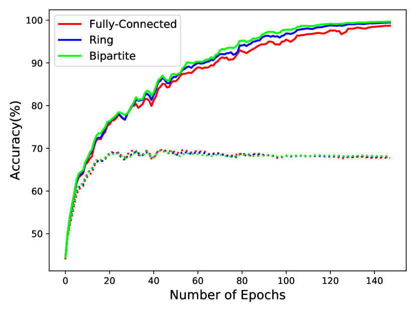
(a)

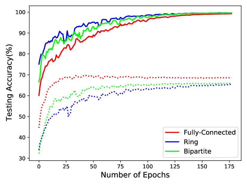
(b)

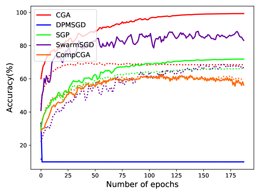
(c)

Figure 5: Average training and validation accuracy for (a) CGA method on IID (b) CGA method on non-IID data distributions (c) different methods on non-IID data distributions for training 5 agents using CNN model architecture

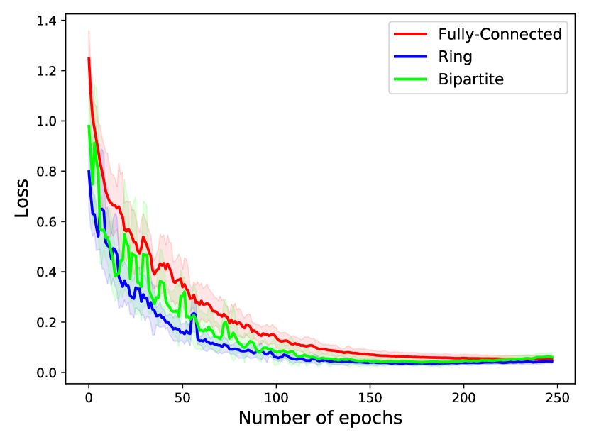
(a)

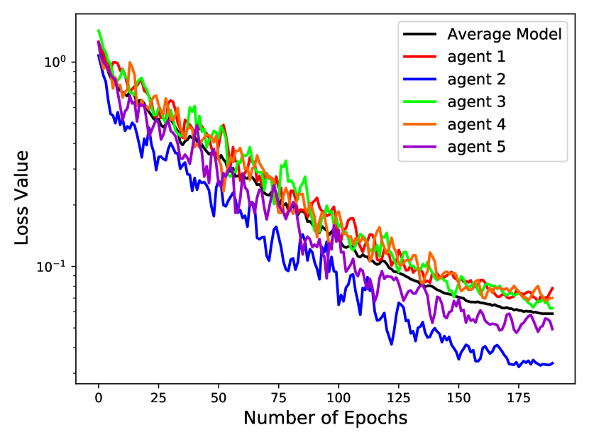
(b)

Figure 6: Average training loss for (a) different topologies trained using CGA algorithm (b) individual agents along with the average model during training using CGA algorithm (log scale)

Based on Figure 5(a), (b) CGA achieves a high accuracy for different graph topologies when learning from both IID and non-IID data distributions. However other methods i.e. DPMSGD suffer from maintaining the high accuracy when learning from non-IID data distributions. The adverse effect of non-IIDness in the data can be more elaborated upon by looking at Figure 7. Comparing (a) with (b) and (c) with (d) we can see that although the migration from IID to non-IID affects all the methods, CGA suffers less than other methods for different combinations of graph topology and graph type. The same observation can be made by looking at Figure 8 which shows the accuracy obtained for different methods w.r.t the graph type.

While Figure 2(a) harps on the phenomenon of faster convergence with sparser graph topology which is an observation that have been made by earlier research works in Federated Learning [McMahan et al., 2017] by reducing the client fraction which makes the mixing matrix sparser and decentralized learning [Jiang et al., 2017]. However, as Figure 6(a) shows, by training for more epochs, all converge to similar loss values. Figure 6 shows that the loss value associated with the consensus model is very close to the loss values corresponding to all other agents which means the projected gradient using QP is capturing the correct direction.

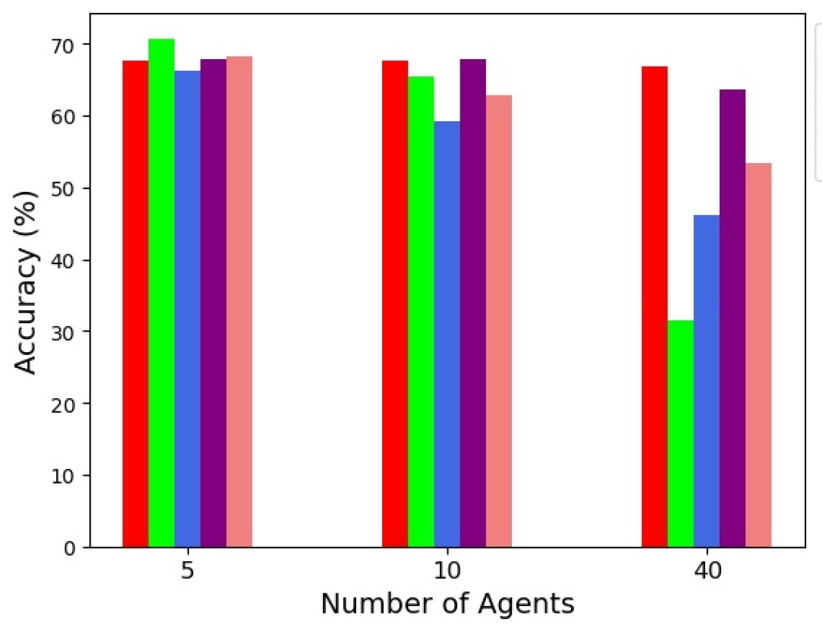
(a)

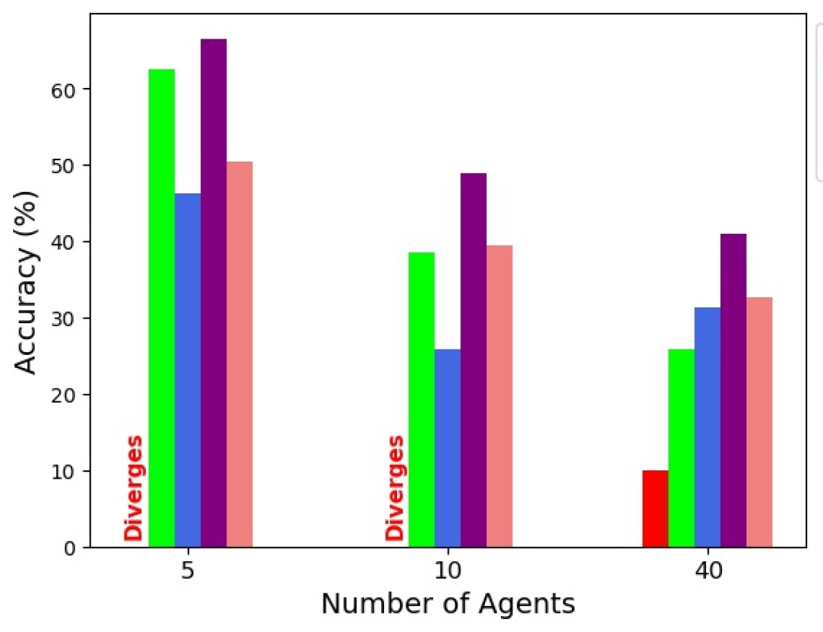
(b)

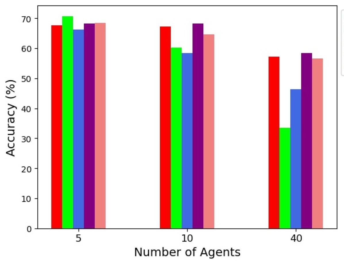
(c)

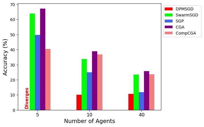
(d)

Figure 7: Average testing accuracy for different methods w.r.t the number of learning agents learning from (a) IID data distributions for Ring graph topology (b) non-IID data distributions for Ring graph topology (c) IID data distributions for Bipartite graph topology (d) non-IID data distributions for Bipartite graph topology

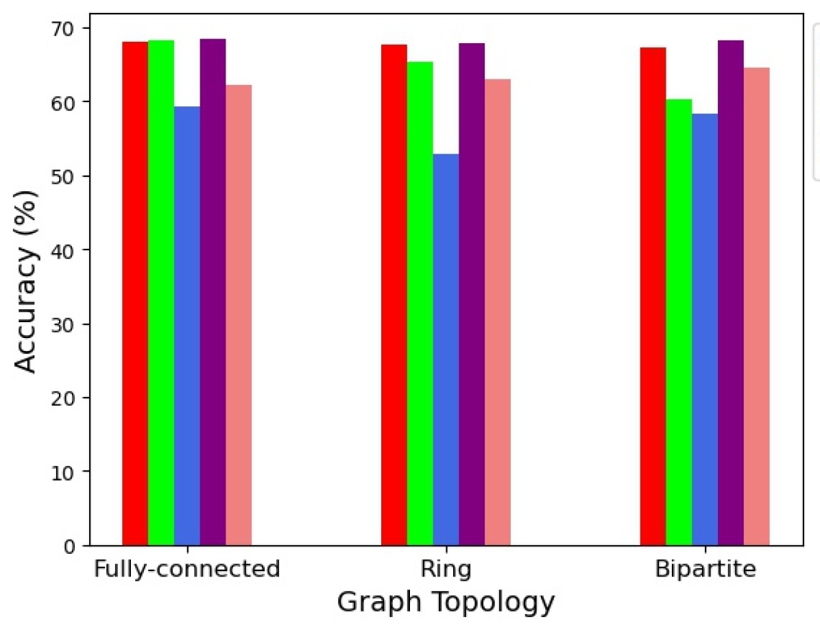
(a)

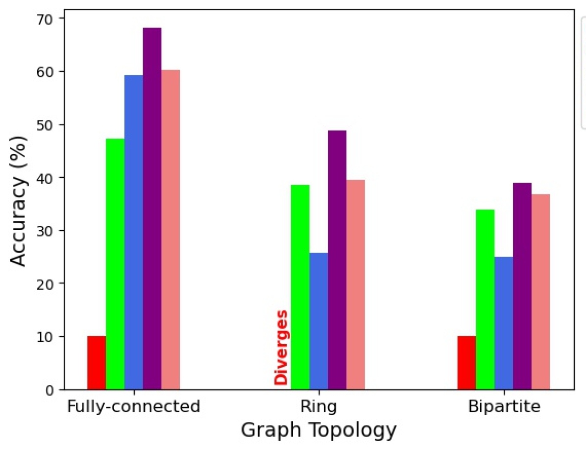
(b)

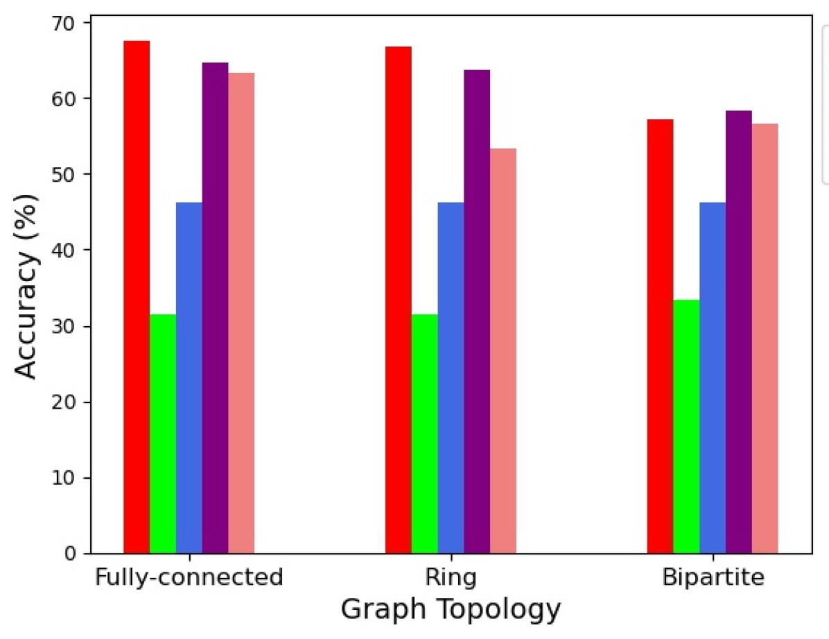
(c)

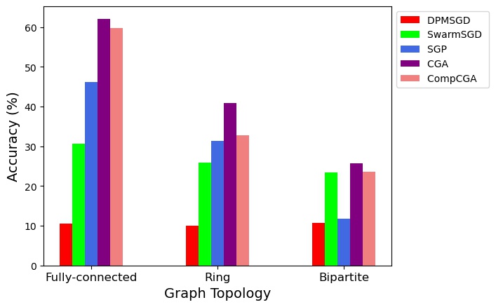
(d)

Figure 8: Average testing accuracy for different methods w.r.t the graph topology learning from (a) IID data distributions learning from 10 agents (b) non-IID data distributions learning from 10 agents(c) IID data distributions learning from 40 agents (d) non-IID data distributions learning from 40 agents

CIFAR10 with VGG11:

We now extend our experimental analysis by using a more complex model architecture (e.g. VGG11) for CIFAR10 dataset. Tables 4 and 5 summarize the performance of CGA compared to other methods. Similar to CNN model architecture, CGA can maintain the performance when migrating from IID to non-IID data distributions. However, we observe that as VGG11 model is much more complex than CNN, all the methods suffer from an increase in the number of learning agents and complexity of graph topology.

Table 4: Model Accuracy Comparison for training CIFAR10 using VGG11 with IID data distribution

Model	Fully-connected	Ring	Bipartite
DPMSGD	67.8% (5) 60.8% (10) 59.8% (40)	61.9% (5) 60.5% (10) 60.1% (40)	61.0% (5) 60.7% (10) 60.1% (40)
SGP	72.5% (5) 70.3% (10) 41.1% (40)	72.0% (5) 42.8% (10) 41.6% (40)	71.1% (5) 70.2% (10) 41.5% (40)
SwarmSGD	75.8% (5) 71.5% (10) 21.8% (40)	73.1% (5) 71.4% (10) 20.6% (40)	78.3% (5) 70.1% (10) 20.3% (40)
CGA (ours)	81.1% (5) 68.8% (10) 21.9% (40)	81.8% (5) 68.3% (10) 18.5% (40)	81.5% (5) 68.2% (10) 20.3% (40)

Table 5: Model Accuracy Comparison for training CIFAR10 with non-IID data distribution using VGG11

Model	Fully-connected	Ring	Bipartite
DPMSGD	Diverges (5) Diverges (10) 12% (40)	Diverges (5) Diverges (10) Diverges (40)	Diverges (5) 10% (10) 10.7% (40)
SGP	20.4% (5) 10.1% (10) Diverges (40)	20.8% (5) 10.0% (10) 10.0% (40)	20.3% (5) Diverges (10) 10.1% (40)
SwarmSGD	19.4% (5) 10.0% (10) 9.9% (40)	19.9% (5) Diverges (10) 10.2% (40)	20.2% (5) Diverges (10) 10% (40)
CGA (ours)	74.6% (5) 69.8% (10) 12.8% (40)	75.8% (5) 38.9% (10) 20.5% (40)	77.5% (5) 18.7% (10) 23.6% (40)

A.6 MNIST Results

Same as what we did for CIFAR-10, we are comparing different methods performance on MNIST dataset. The results are summarized in Tables 6 and 7. Although the accuracies are generally high when learning from MNIST dataset, and most of the methods work in most of the settings, we can see that although CGA can maintain the model performance while learning from non-IID data, DPMSGD, SGP and SwarmSGD suffer from non-IIDness in the data specially when the number of agents and the graph topology combinations become more complex.

Table 6: Model Accuracy Comparison for training MNIST using CNN with IID data distribution

Model	Fully-connected	Ring	Bipartite
DPSGD	98.8% (5) 98.6% (10) 96.9% (40)	98.8% (5) 98.5% (10) 96.8% (40)	98.8% (5) 98.5% (10) 96.8% (40)
SGP	96.2% (5) 93.2% (10) 71.4% (40)	96.3% (5) 93.2% (10) 71.4% (40)	96.2% (5) 93.2% (10) 71.4% (40)
SwarmSGD	98.4% (5) 96.1% (10) 38.3% (40)	98.4% (5) 96.1% (10) 38.3% (40)	98.5% (5) 96.0% (10) 39.7% (40)
CGA (ours)	98.6 % (5) 98.2% (10) 94.7% (40)	98.7% (5) 98.3% (10) 95.5% (40)	98.7% (5) 98.6% (10) 96.8% (40)

Table 7: Model Accuracy Comparison for training MNIST with non-IID data distribution using CNN

Model	Fully-connected	Ring	Bipartite
DPSGD	98.3% (5) 87.1% (10) 85.3% (40)	98.2% (5) 74.5% (10) 72.5% (40)	98.2% (5) 70.9% (10) 34.3% (40)
SGP	95.9% (5) 92.7% (10) 71.2% (40)	96.0% (5) 91.3% (10) 74.6% (40)	95.9% (5) 90.2% (10) 62.2% (40)
SwarmSGD	98.2% (5) 93.2% (10) 24.8% (40)	98.1% (5) 90.9% (10) 33.5% (40)	98.2% (5) 91.4% (10) 18.3% (40)
CGA (ours)	98.6% (5) 98.2% (10) 94.1% (40)	98.5% (5) 96.2% (10) 91.6% (40)	98.5% (5) 96.2% (10) 91.8% (40)

References

• Alistarh et al. (2018) Dan Alistarh, Torsten Hoefler, Mikael Johansson, Nikola Konstantinov, Sarit Khirirat, and Cédric Renggli. The convergence of sparsified gradient methods. In Advances in Neural Information Processing Systems, pages 5973–5983, 2018.
• Arjevani et al. (2020) Yossi Arjevani, Joan Bruna, Bugra Can, Mert Gürbüzbalaban, Stefanie Jegelka, and Hongzhou Lin. Ideal: Inexact decentralized accelerated augmented lagrangian method. arXiv preprint arXiv:2006.06733, 2020.
• Assran et al. (2019) Mahmoud Assran, Nicolas Loizou, Nicolas Ballas, and Mike Rabbat. Stochastic gradient push for distributed deep learning. In International Conference on Machine Learning, pages 344–353. PMLR, 2019.
• Balu et al. (2021) Aditya Balu, Zhanhong Jiang, Sin Yong Tan, Chinmay Hedge, Young M Lee, and Soumik Sarkar. Decentralized deep learning using momentum-accelerated consensus. In ICASSP 2021-2021 IEEE International Conference on Acoustics, Speech and Signal Processing (ICASSP), pages 3675–3679. IEEE, 2021.
• Boyd et al. (2006) Stephen Boyd, Arpita Ghosh, Balaji Prabhakar, and Devavrat Shah. Randomized gossip algorithms. IEEE transactions on information theory, 52(6):2508–2530, 2006.
• Dekel et al. (2012) Ofer Dekel, Ran Gilad-Bachrach, Ohad Shamir, and Lin Xiao. Optimal distributed online prediction using mini-batches. The Journal of Machine Learning Research, 13:165–202, 2012.
• Haghighat et al. (2020) Arya Ketabchi Haghighat, Varsha Ravichandra-Mouli, Pranamesh Chakraborty, Yasaman Esfandiari, Saeed Arabi, and Anuj Sharma. Applications of deep learning in intelligent transportation systems. Journal of Big Data Analytics in Transportation, 2(2):115–145, 2020.
• Hsieh et al. (2019) Kevin Hsieh, Amar Phanishayee, Onur Mutlu, and Phillip B Gibbons. The non-iid data quagmire of decentralized machine learning. arXiv preprint arXiv:1910.00189, 2019.
• Jiang et al. (2017) Zhanhong Jiang, Aditya Balu, Chinmay Hegde, and Soumik Sarkar. Collaborative deep learning in fixed topology networks. Advances in Neural Information Processing Systems, 2017:5905–5915, 2017.
• Jiang et al. (2018) Zhanhong Jiang, Aditya Balu, Chinmay Hegde, and Soumik Sarkar. On consensus-optimality trade-offs in collaborative deep learning. arXiv preprint arXiv:1805.12120, 2018.
• Kairouz et al. (2019) Peter Kairouz, H Brendan McMahan, Brendan Avent, Aurélien Bellet, Mehdi Bennis, Arjun Nitin Bhagoji, Keith Bonawitz, Zachary Charles, Graham Cormode, Rachel Cummings, et al. Advances and open problems in federated learning. arXiv preprint arXiv:1912.04977, 2019.
• Karimireddy et al. (2019a) Sai Praneeth Karimireddy, Satyen Kale, Mehryar Mohri, Sashank J Reddi, Sebastian U Stich, and Ananda Theertha Suresh. Scaffold: Stochastic controlled averaging for on-device federated learning. arXiv preprint arXiv:1910.06378, 2019a.
• Karimireddy et al. (2019b) Sai Praneeth Karimireddy, Quentin Rebjock, Sebastian U Stich, and Martin Jaggi. Error feedback fixes signsgd and other gradient compression schemes. arXiv preprint arXiv:1901.09847, 2019b.
• Kempe et al. (2003) David Kempe, Alin Dobra, and Johannes Gehrke. Gossip-based computation of aggregate information. In 44th Annual IEEE Symposium on Foundations of Computer Science, 2003. Proceedings., pages 482–491. IEEE, 2003.
• Koloskova et al. (2019) Anastasia Koloskova, Tao Lin, Sebastian U Stich, and Martin Jaggi. Decentralized deep learning with arbitrary communication compression. arXiv preprint arXiv:1907.09356, 2019.
• Koloskova et al. (2020) Anastasia Koloskova, Nicolas Loizou, Sadra Boreiri, Martin Jaggi, and Sebastian U Stich. A unified theory of decentralized sgd with changing topology and local updates. arXiv preprint arXiv:2003.10422, 2020.
• Konečnỳ et al. (2016) Jakub Konečnỳ, H Brendan McMahan, Daniel Ramage, and Peter Richtárik. Federated optimization: Distributed machine learning for on-device intelligence. arXiv preprint arXiv:1610.02527, 2016.
• Li et al. (2019a) Chengjie Li, Ruixuan Li, Haozhao Wang, Yuhua Li, Pan Zhou, Song Guo, and Keqin Li. Gradient scheduling with global momentum for non-iid data distributed asynchronous training. arXiv preprint arXiv:1902.07848, 2019a.
• Li et al. (2018) Tian Li, Anit Kumar Sahu, Manzil Zaheer, Maziar Sanjabi, Ameet Talwalkar, and Virginia Smith. Federated optimization in heterogeneous networks. arXiv preprint arXiv:1812.06127, 2018.
• Li et al. (2019b) Xiang Li, Kaixuan Huang, Wenhao Yang, Shusen Wang, and Zhihua Zhang. On the convergence of fedavg on non-iid data. arXiv preprint arXiv:1907.02189, 2019b.
• Lian et al. (2017) Xiangru Lian, Ce Zhang, Huan Zhang, Cho-Jui Hsieh, Wei Zhang, and Ji Liu. Can decentralized algorithms outperform centralized algorithms? a case study for decentralized parallel stochastic gradient descent. In Advances in Neural Information Processing Systems, pages 5330–5340, 2017.
• Lopez-Paz and Ranzato (2017) David Lopez-Paz and Marc’Aurelio Ranzato. Gradient episodic memory for continual learning. In Advances in Neural Information Processing Systems, pages 6467–6476, 2017.
• Lu and De Sa (2020) Yucheng Lu and Christopher De Sa. Moniqua: Modulo quantized communication in decentralized sgd. arXiv preprint arXiv:2002.11787, 2020.
• McMahan et al. (2017) Brendan McMahan, Eider Moore, Daniel Ramage, Seth Hampson, and Blaise Aguera y Arcas. Communication-efficient learning of deep networks from decentralized data. In Artificial Intelligence and Statistics, pages 1273–1282. PMLR, 2017.
• Nadiradze et al. (2019) Giorgi Nadiradze, Amirmojtaba Sabour, Dan Alistarh, Aditya Sharma, Ilia Markov, and Vitaly Aksenov. SwarmSGD: Scalable decentralized SGD with local updates. arXiv preprint arXiv:1910.12308, 2019.
• Nedić et al. (2018) Angelia Nedić, Alex Olshevsky, and Michael G Rabbat. Network topology and communication-computation tradeoffs in decentralized optimization. Proceedings of the IEEE, 106(5):953–976, 2018.
• Nesterov (2012) Yu Nesterov. Efficiency of coordinate descent methods on huge-scale optimization problems. SIAM Journal on Optimization, 22(2):341–362, 2012.
• Richtárik and Takáč (2016) Peter Richtárik and Martin Takáč. Distributed coordinate descent method for learning with big data. The Journal of Machine Learning Research, 17(1):2657–2681, 2016.
• Rothchild et al. (2020) Daniel Rothchild, Ashwinee Panda, Enayat Ullah, Nikita Ivkin, Ion Stoica, Vladimir Braverman, Joseph Gonzalez, and Raman Arora. Fetchsgd: Communication-efficient federated learning with sketching. arXiv preprint arXiv:2007.07682, 2020.
• Sattler et al. (2019) Felix Sattler, Simon Wiedemann, Klaus-Robert Müller, and Wojciech Samek. Robust and communication-efficient federated learning from non-iid data. IEEE transactions on neural networks and learning systems, 2019.
• Scaman et al. (2018) Kevin Scaman, Francis Bach, Sébastien Bubeck, Laurent Massoulié, and Yin Tat Lee. Optimal algorithms for non-smooth distributed optimization in networks. In Advances in Neural Information Processing Systems, pages 2740–2749, 2018.
• Seide et al. (2014) Frank Seide, Hao Fu, Jasha Droppo, Gang Li, and Dong Yu. 1-bit stochastic gradient descent and its application to data-parallel distributed training of speech dnns. In Fifteenth Annual Conference of the International Speech Communication Association, 2014.
• Shoham et al. (2019) Neta Shoham, Tomer Avidor, Aviv Keren, Nadav Israel, Daniel Benditkis, Liron Mor-Yosef, and Itai Zeitak. Overcoming forgetting in federated learning on non-iid data. arXiv preprint arXiv:1910.07796, 2019.
• Simonyan and Zisserman (2014) Karen Simonyan and Andrew Zisserman. Very deep convolutional networks for large-scale image recognition. arXiv preprint arXiv:1409.1556, 2014.
• Tang et al. (2019) Hanlin Tang, Xiangru Lian, Shuang Qiu, Lei Yuan, Ce Zhang, Tong Zhang, and Ji Liu. Deepsqueeze: Parallel stochastic gradient descent with double-pass error-compensated compression. CoRR, abs/1907.07346, 2019. URL http://arxiv.org/abs/1907.07346.
• Tong et al. (2020) Qianqian Tong, Guannan Liang, and Jinbo Bi. Effective federated adaptive gradient methods with non-iid decentralized data. arXiv preprint arXiv:2009.06557, 2020.
• Vogels et al. (2020) Thijs Vogels, Sai Praneeth Karimireddy, and Martin Jaggi. Practical low-rank communication compression in decentralized deep learning. Advances in Neural Information Processing Systems, 33, 2020.
• Wang et al. (2019) Jianyu Wang, Vinayak Tantia, Nicolas Ballas, and Michael Rabbat. Slowmo: Improving communication-efficient distributed sgd with slow momentum. arXiv preprint arXiv:1910.00643, 2019.
• Wang et al. (2020) Jianyu Wang, Qinghua Liu, Hao Liang, Gauri Joshi, and H Vincent Poor. Tackling the objective inconsistency problem in heterogeneous federated optimization. arXiv preprint arXiv:2007.07481, 2020.
• Xiao and Boyd (2004) Lin Xiao and Stephen Boyd. Fast linear iterations for distributed averaging. Systems & Control Letters, 53(1):65–78, 2004.
• Yu et al. (2019) Hao Yu, Rong Jin, and Sen Yang. On the linear speedup analysis of communication efficient momentum sgd for distributed non-convex optimization. arXiv preprint arXiv:1905.03817, 2019.
• Zhao et al. (2018) Yue Zhao, Meng Li, Liangzhen Lai, Naveen Suda, Damon Civin, and Vikas Chandra. Federated learning with non-iid data. arXiv preprint arXiv:1806.00582, 2018.