EnD: Entangling and Disentangling deep representations for bias correction

Abstract

Artificial neural networks perform state-of-the-art in an ever-growing number of tasks, and nowadays they are used to solve an incredibly large variety of tasks. There are problems, like the presence of biases in the training data, which question the generalization capability of these models. In this work we propose EnD, a regularization strategy whose aim is to prevent deep models from learning unwanted biases. In particular, we insert an “information bottleneck” at a certain point of the deep neural network, where we disentangle the information about the bias, still letting the useful information for the training task forward-propagating in the rest of the model. One big advantage of EnD is that we do not require additional training complexity (like decoders or extra layers in the model), since it is a regularizer directly applied on the trained model. Our experiments show that EnD effectively improves the generalization on unbiased test sets, and it can be effectively applied on real-case scenarios, like removing hidden biases in the COVID-19 detection from radiographic images.

1 Introduction

In the last two decades artificial neural network models (ANNs) received huge interest from the research community. Nowadays, complex and even ill-posed problems can be tackled provided that one can train a deep enough ANN model with a large enough dataset. Furthermore, they aim to become a powerful tool helping us take a variety of decisions: for example, AI is currently used for scouting and hiring people [17]. These ANNs are trained to process a desired output from some inputs. We have no clear idea how the information is effectively processed inside. Recently, AI trustworthiness has been recognized as major prerequisite for people and societies to use and accept such systems [14, 33]. In April 2019, the High-Level Expert Group on AI of the European Commission defined the three main aspects of trustworthy AI [14]: it should be lawful, ethical and robust. Providing a warranty on this topic is currently a matter of study and discussion.
Focusing on the concept of robustness for AI, Attenberg et al. discussed the problem of finding the so-called “unknown unknowns” [3] in data. These unknown unknowns relate to the case when the deep model elaborates information in an unintended way, but shows high confidence on its predictions. Such behavior affected many recent works proposing AI-based solutions on the COVID detection from radiographic images. Unfortunately, the available datasets at the beginning of the pandemic were heavily biased. This often resulted in models predicting COVID diagnosis with a high confidence, thanks to the presence of unwanted biases, for example by detecting the presence of catheters or medical devices for positive patients, their age (at the beginning of the pandemic, most ill patients were elderly people), or even by recognizing the origin of the data itself (when negative cases were augmented borrowing samples from other datasets) [2, 25, 26].
In this work we propose a regularization strategy which Entangles the deep features extracted by patterns belonging to the same target class and Disentangles the biased features: we name it EnD, and with it we wish to put an end to the bias propagation in any deep model. We assume we know data might have some bias (like in the case of COVID, the origin of data) but we ignore what it translates into (we do not have a prior knowledge on whether the bias is the presence of some color, a specific feature in the image or anything else). EnD regularizes the output of some layer $\Gamma$ within the deep model in order to create an “information bottleneck” where the regularizer:

• entangles the feature vectors extracted from data belonging to the same target class;

• disentangles the features extracted from data having the same “bias label”.

Since the deep model is trained minimizing both the loss and EnD, all the biased features are discouraged to be extracted in favor of the unbiased ones. Compared to other de-biasing techniques, we have no training overhead: we do not train extra models to perform gradient inversion on the biased information or involve the use of GaNs, or even de-bias the input data. EnD works directly on the target model, and is minimized via standard back-propagation.
In general, directly tackling the problem of mutual information’s minimization is hard, given both its non-differentiability and the computational complexity involved. Nonetheless, previous works have already shown that adding further constraints to the learning problem could be effective [28] as, typically, the trained ANN models are over-sized and allows a large number of solutions to the same learning task [27]. Our experiments show that EnD effectively favors the choice of unbiased features over the biased ones at training time, yielding competitive generalization capabilities compared to models trained with other un-biasing techniques.
The rest of the work is structured as follows. In Sec. 2 we review some works close to our problem. Then, in Sec. 3 we introduce EnD in detail providing intuitions on its effect. Sec. 4 shows some empirical results and finally, in Sec. 5, the conclusions are drawn.

2 Related works

In this section we review state-of-the-art techniques designed to prevent models from learning biases. The techniques can be grouped into (but not limited to) three main approaches: direct data de-biasing from the source, use of GANs/ensembling towards data de-biasing and direct learning the de-biasing within the trained model.
De-biasing from data source It is known that datasets are typically affected by biases. In their work, Torralba and Efros [30] showed how biases affect some of the most commonly used datasets, drawing considerations on the generalization performance and classification capability of the trained ANN models. Following a similar approach, Tommasi et al. [29] conducted experiments reporting differences between a number of datasets and verifying how final performances vary when applying different de-biasing strategies in order to balance data. Working at the dataset level is in general a critical aspect, and greatly helps in understanding the data and its structure [8]. The concept of removing bias by using data borrowed by different sources has been explored in a practical and empirical context by Gupta et al. [11]. In particular, they have designed a de-biasing strategy to minimize the effects of imperfect execution and calibration errors by reducing the effect of unbalanced data, showing improvements in the generalization of the final model.

Adversarial and ensembling approaches. Having an explicit formulation for the bias contribution in the loss term is typically hard. One possible approach is to use additional models to learn the biases in data and use them to condition the primary model so that it avoids them. Kim et al. use adversarial learning and gradient inversion to eliminate the information related to the biases in the model [16]. Another possibility is to use the gray-level co-occurence matrix to extract unbiased features and to train the model, as proposed by Wang et al. with HEX [32]. Alvi et al. propose the BlindEye [1] technique, where they train a classifier on the extracted deep features to retrieve information from biases: then, they force the “bias classifier” to be no longer able to retrieve bias-related information, modifying the deep features accordingly. Bahng et al. [4] develop an ensembling-based technique, called ReBias. It consists in solving a min-max problem where the target is to promote the independence between the network prediction and all biased predictions. Identifying the “known unknowns” [3] and optimize on those using a neural networks ensemble is the approach proposed by Nam et al. with their LfF [21]. A similar approach is followed by Clark et al. in their LearnedMixin [6].

De-biasing within the deep model. Dataset de-biasing helps in the learning process, as training is performed with no biases; however, with such an approach we typically have no direct control on the information we are removing from the dataset itself, or we are including an extremely-high computational complexity like when training GANs. A context in which, on the contrary, we can have direct access to these biases is presented by Hendricks et al. [13]. In such a work it was possible to explicitly introduce a corrective loss term (coherent with the formulation introduced by Vinyals et al. [31]) with the aim to help the ANN model to focus on the correct features. Similarly, Cadene et al. propose RUBi [5] where they use logit re-weighting to lower the bias impact in the learning process, and Sagawa et al., with Group-DRO [23], avoid bias overfitting by defining prior data sub-groups and controlling their generalization. EnD belongs to this class of approaches, since we directly regularize the trained model, with no additional parameters to be learned. In Sec. 3 we are going to describe in detail the approach we take in order to EnD bias propagation in the trained model.

3 Entangling and Disentangling deep representations

Figure 1: Model overview. The features for EnD are extracted at the output of $\Gamma$, after a normalization layer performing the operation as in (3).

(a)

(b)

Figure 2: Toy example of EnD’s effect. Each arrow represents the feature vector associated with a sample. Biases are represented by the three different colors (green, orange and blue) while the target class is represented by the arrows marker’s symbol (triangle, square and circle). While in some un-regularized training the deep model strongly correlates with the bias (a), using EnD we aim at enforcing the choices of different features (b).

In this section, after introducing the notation, we present EnD, our proposed regularization term, whose aim is to regularize the deep features in order to discourage the deep model to learn biases.

3.1 Preliminaries

In this section we first introduce the notation we are going to use for the rest of this work and we provide some intuitions on how EnD is going to work. Let us assume we focus our attention on some layer $\Gamma$, at the output of which we are going to apply EnD. Let $T$ be the cardinality of the target classes of the learning problem and $B$ the cardinality of the bias classes in the dataset. We say the output of $\Gamma$ is $\boldsymbol{y}~{}\in~{}\mathbb{R}^{N_{\Gamma}\times M}$, where $M$ is the batchsize and $N_{\Gamma}$ is the output size of $\Gamma$.
We also define:

• $M^{t,b}$ as the cardinality of the samples having the same target $t$ and the same bias $b$;

• $M^{t,-}$ as the cardinality of the samples having the same target $t$ regardless the biases;

• $M^{-,b}$ as the cardinality of the samples having the same bias $b$ regardless the target class;

• $\boldsymbol{y}^{t,b}$ as the subset of the features $\boldsymbol{y}$ belonging to the inputs having the same target class $t$ and showing the same bias $b$;

• $\boldsymbol{y}^{t,-}$ as the subset of the features $\boldsymbol{y}$ belonging to the inputs having the same target class $t$ regardless the bias;

• $\boldsymbol{y}^{-,b}$ as the subset of the features $\boldsymbol{y}$ belonging to the inputs having the same bias $b$ regardless the target class;

• $\boldsymbol{y}_{i}$ as the $i$-th sample in the minibatch;

• $\mathcal{T}(\boldsymbol{y}_{i})$ extracts the target class of $\boldsymbol{y}_{i}$;

• $\mathcal{B}(\boldsymbol{y}_{i})$ extracts the bias class of $\boldsymbol{y}_{i}$.

In our work, EnD sides the loss minimization, discouraging the selection of biased deep features and encouraging the unbiased ones at training time. Hence, the overall objective function we aim to minimize is

$$J=L+R,$$ (1)

where $L$ is the loss function for the trained task and $R$ is our proposed EnD term, applied at the output of $\Gamma$. Fig. 1 provides the overall structure of the trained model.
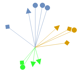
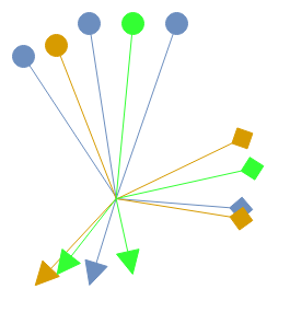
Let us consider, as a toy example, some classification problem having three target classes, but as well three different bias classes (Fig. 2 shows the extracted feature vectors at $\Gamma$). We encode the biases as three different colors (green, orange and blue), while the target class is represented by the arrows marker (triangle, square and circle). Typically, training a deep model without taking biases into account produces feature representations shown in Fig. 2a: here, the loss on the target classes is minimized (three distinct groups are formed depending on the arrow marker), but it is driven by a heavy bias (the colors of the arrows). The purpose of EnD is to disentangle the representations belonging to the same bias class (color) and to entangle the representations with the same target class (the arrow’s marker). Fig. 2b represents the effect of EnD on the deep representations: while the disentangling term un-groups the biased example’s representations, i.e. makes corresponding vectors almost orthogonal, the entangling one promotes correlations between samples having the same target.

3.2 Data correlations

Our main goal is to train our model to correctly classify the data into the $T$ possible classes, preventing the use of the bias features provided in the data. Towards this end, we aim at inserting an information bottleneck: the information related to these biases will be used as little as possible for the target classification task.
We can build a similarity matrix $G\in\mathbb{R}^{M\times M}$:

$$G=\left(\tilde{\boldsymbol{y}}\right)^{\prime}\cdot\tilde{\boldsymbol{y}},$$ (2)

where $(\cdot)^{\prime}$ indicates transposed matrix and $\tilde{\boldsymbol{y}}$ indicates a per-representation normalization

$$\tilde{\boldsymbol{y}}_{i}=\frac{\boldsymbol{y}_{i}}{\|\boldsymbol{y}_{i}\|_{2}}\forall i\in[1,M].$$ (3)

Hence, every $g_{i,j}$ entry between two patterns $i,j$ in $G$ indicates their correlation:

$$g_{i,j}=\left(\tilde{\boldsymbol{y}}_{i}\right)^{\prime}\cdot\tilde{\boldsymbol{y}}_{j}.$$ (4)

$G$ is a special case of Gramian matrix, as any $g_{i,j}~{}\in~{}[-1;+1]$ and indicates the difference in the direction between any two $\boldsymbol{y}_{i}$ and $\boldsymbol{y}_{j}$. $G$ has some properties:

• is a symmetric, positive semi-definite matrix;

• all the elements in the main diagonal are exactly $1$ by construction;

• if the subset of outputs $\tilde{\mathbf{y}}$ forms an ortho-normal basis (or $G$ is full-rank), then $G=\mathbb{I}$ by definition.

Handling these relations, we are going to build our regularization strategy, which consists in two terms:

• a disentangling term, whose task is to try to de-correlate as much as possible all the patterns belonging to the same bias class $b$;

• an entangling term, which attempts to force correlations between data from different bias classes but having the same target class $t$.

3.3 The EnD regularizer

The regularization $R$ we propose blends the disentangling $R_{\perp}$ and entangling $R_{\parallel}$ terms by setting

$$R=\alpha R_{\perp}+\beta R_{\parallel},$$ (5)

where $\alpha$ and $\beta$ are proper multipliers. In the following, we are going to describe in detail the disentangling and the entangling terms.

3.3.1 Disentangling term

In order to disentangle biased representations, at training time, we select the patterns belonging to a bias class $b$ and build the corresponding Gramian matrix

$$G^{-,b}=\left(\tilde{\boldsymbol{y}}^{-,b}\right)^{\prime}\cdot\tilde{\boldsymbol{y}}^{-,b}.$$ (6)

Then, we enforce de-correlation between the features belonging to the same class: ideally, we would like to get $G^{-,b}~{}\rightarrow~{}\mathbb{I}~{}\forall~{}b$. To this end, we introduce the regularization term

$$R_{\perp}=\frac{1}{B}\sum_{b=1}^{B}\frac{1}{\left(M^{-,b}\right)^{2}}\sum_{i,j}\left|g_{i,j}^{-,b}\right|$$ (7)

that promotes minimization of the off-diagonal elements in $G^{-,b}$, $\forall b$.

3.3.2 Entangling term

While $R_{\perp}$ discourages the model to learn biases, the model should also build strong correlations between patterns belonging to different bias classes, but to the same target class $t$. With an orthogonal approach to the one used to derive (6), we compute the Gramian matrix for the patterns belong to the same target class $t$:

$$G^{t,-}=\left(\tilde{\boldsymbol{y}}^{t,-}\right)^{\prime}\cdot\tilde{\boldsymbol{y}}^{t,-}.$$ (8)

Let us focus, now, on the vector $\boldsymbol{g}_{i}^{t,-}$, extracted from the $i$-th column of $G^{t,-}$: it expresses how the $i$-th pattern correlates to all the other patterns which will be grouped to the same $t$-th target class. As a first option, we might ask the model to correlate the $i$-th pattern to all the other patterns having the same target class $t$, deriving the pattern entangling rule as the opposite of the disentangling rule in (7):

$$\hat{R}_{\parallel}=1-\frac{1}{T}\sum_{t=1}^{T}\frac{1}{\left(M^{t,-}\right)^{2}}\sum_{i,j}g_{i,j}^{t,-}$$ (9)

In this formulation we are asking all the $g_{i,j}^{t,-}\rightarrow 1$, correlating the features as much as possible. However, (9) has a major shortcoming: it simply forces again correlations according to the target class $t$ regardless the bias information, which might be re-introduced. This is already done at a more general level by the loss function minimization as in (1): it is desirable to have a term which entangles features having the same target class, but belonging to different bias classes. Towards this end, we can re-write (9) maximizing the correlations between each single example $\boldsymbol{y}_{i}$ and every other example $\boldsymbol{y}_{j}$ such that $\mathcal{T}(\boldsymbol{y}_{i})=\mathcal{T}(\boldsymbol{y}_{j})$ but, at the same time, $\mathcal{B}(\boldsymbol{y}_{i})\neq\mathcal{B}(\boldsymbol{y}_{j})$. Hence, our entangling term reads

$$R_{\parallel}=1-\frac{1}{M}\sum_{i=1}^{M} \frac{1}{\sum\limits_{b\neq\mathcal{B}(\boldsymbol{y}_{i})}M^{\mathcal{T}(\boldsymbol{y}_{i}),b}}\cdot$$

$$\cdot \sum_{j}\bar{\delta}\left[\mathcal{B}(\boldsymbol{y}_{i}),\mathcal{B}(\boldsymbol{y}_{j})\right]\cdot{g}_{i,j}^{\mathcal{T}(\boldsymbol{y}_{i}),-},$$ (10)

where

$$\bar{\delta}(a,b)=\left\{\begin{array}[]{ll}0&a=b\\ 1&a\neq b\end{array}\right..$$ (11)

4 Experiments

In the experiments we present in this section, we aim to remove different types of biases such as color, age, gender which can have a high impact on classification performance when recognizing, for example, attributes such as hair color and presence of makeup on facial images. Additionally, we also show how this technique can help in sensitive tasks such as in the medical field, specifically in COVID-19 detection from CXR images. In all the results tables, the best results are denoted as boldface, the second best results are underlined. “Vanilla” denotes the baseline model performance for the learning problem, with no debiasing technique applied. All the EnD’s results are averaged over three different runs.

4.1 Controlled experiments

In this section we describe the controlled experiments that we performed in order to assess the performance of EnD. Full control over the amount and type of bias allows to correctly analyze EnD’s behavior, excluding noise and uncertainty given by real-world data.

4.1.1 Biased MNIST

Figure 3: Biased MNIST by Bahng et al. [4], where the background colors highly correlate with the digit classes.

Method	$\rho$ values
	0.999	0.997	0.995	0.990
Vanilla	10.4	33.4	72.1	89.1
HEX [32]	10.8	16.6	19.7	24.7
LearnedMixin [6]	12.1	50.2	78.2	88.3
RUBi [5]	13.7	43.0	90.4	93.6
ReBias [4]	22.7	64.2	76.0	88.1
EnD	52.30	83.70	93.92	96.02
	$\pm$ 2.39	$\pm$ 1.03	$\pm$ 0.35	$\pm$ 0.08

Table 1: Biased MNIST performance on the unbiased test set.

(a)  

(b)  

Figure 4: Grad-CAM on Colored MNIST: [24] vanilla model (a) and EnD-regularized model (b).

(a)  

(b)  

(c)  

(d)  

Figure 5: EnD learning curves on Colored MNIST for $\boldsymbol{\rho}\mathbf{=0.995}$. Biased accuracy (a), unbiased accuracy (b), $L$ value on the training set (c) and $R$ value on the training set (d).

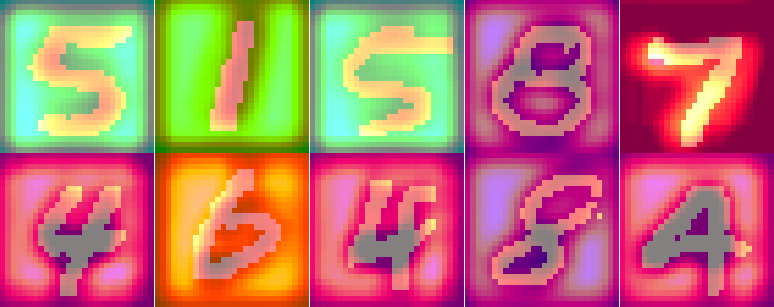
We test our method on a synthetic dataset, where we can control the bias in the training data. We use the Biased MNIST dataset proposed by Bahng et al. [4]. This dataset is constructed from the MNIST dataset [18] by injecting a color into the images background, as shown in Figure 3. Each digit is associated with one of ten pre-defined colors. To assign the color bias to an image of a given target class, the pre-defined color is selected with a probability $\rho$, and any other color is chosen with a probability $(1-\rho)$. To vary the level of difficulty in the dataset, the authors select $\rho\in\{0.990,0.995,0.997,0.999\}$. Higher values of $\rho$ correspond to higher correlation between target class and bias class (color). Two testing datasets are constructed with the same criterion: biased, with $\rho=1.0$, and unbiased, with $\rho=0.1$. Given the low correlation between color and digit class in the unbiased test set, models must learn to classify shapes instead of colors in order to reach a high accuracy.

Setup. We use the network architecture proposed by Bahng et al. [4], consisting of four convolutional layers with $7\times 7$ kernels. The EnD regularization term is applied on the average pooling layer, before the fully connected classifier of the network.

Results. Results are shown in Table 1. EnD’s results are averaged across three different runs for each value of $\rho$. For all values of $\rho$ we report the accuracy obtained by EnD on the unbiased evaluation set, compared with other debiasing algorithms.

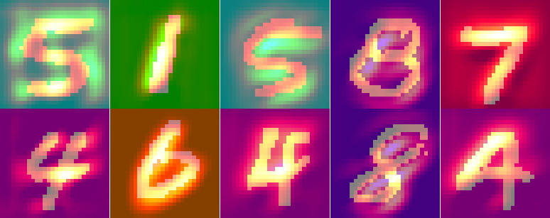
EnD successfully mitigates bias propagation. The improvement obtained with EnD with respect to the baseline model is noticeable, especially in the higher levels of difficulty. We observe an increase of accuracy across all values of $\rho$. Notably, for $\rho=0.999$ the vanilla model reaches 10.4% accuracy, meaning that the background color is used as the only cue for classifying the digits, whereas employing EnD yields an accuracy of 52.30%. Figure 4 shows the effect of EnD, using Grad-CAM [24] to highlight the important regions of the input image for the model prediction. We observe that the vanilla model (Figure 4(a)) focuses on the background, while the EnD-regularized model (Figure 4(b)) correctly learns to focus on the digit shape.

Comparison with other techniques. We observe that EnD yields the highest results among all of the compared debiasing algorithms. Such gap is especially higher in the most difficult settings for $\rho\in\{0.999,0.997\}$ where many algorithms are unable to generalize to the unbiased set, especially HEX [32] and LearnedMixin [6]. Some of the compared algorithms even show a collapse in accuracy compared to the vanilla baseline in certain cases (HEX for most values of $\rho$, LearnedMixin and ReBias for $\rho=0.990$).

Ablation study. We also perform an ablation study of EnD to analyze how each of the EnD’s terms affect the performance of the trained model. For a fixed $\rho=0.997$, we evaluate only the contribution of the disentangling term $R_{\perp}$ and disable the entangling term $R_{\parallel}$ by setting $\beta=0$. We then perform the opposite evaluation by setting $\alpha=0$, to only take into account the entangling term.

Setting	$\alpha$	$\beta$	Unbiased
			accuracy
Vanilla	0	0	33.4
Disentangling only	$[0;1]$	0	45.67 $\pm$ 0.67
Entangling only	0	$[0;1]$	75.36 $\pm$ 0.94
EnD	$[0;1]$	$[0;1]$	83.70 $\pm$ 1.03

Table 2: Ablation study of EnD on the Biased MNIST dataset, $\rho=0.997$.

The results are shown in Table 2. We observe that both the regularization terms contribute to boost the model’s generalization capability. As expected, the best results are achieved when both of them are jointly applied. The entangling term yields a higher increase in performance compared to the disentangling one, however it is in general not always applicable, for example when, given some $i$-th sample $\boldsymbol{y}_{i}$,

$$\nexists j~{}|~{}\mathcal{T}(\boldsymbol{y}_{i})=\mathcal{T}(\boldsymbol{y}_{j})\land\mathcal{B}(\boldsymbol{y}_{i})\neq\mathcal{B}(\boldsymbol{y}_{j})~{}\forall i.$$

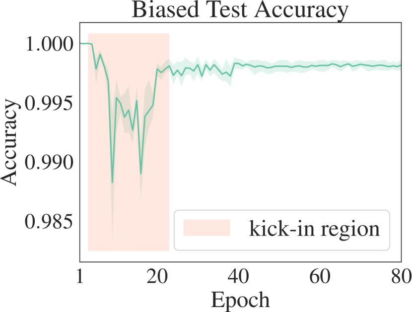
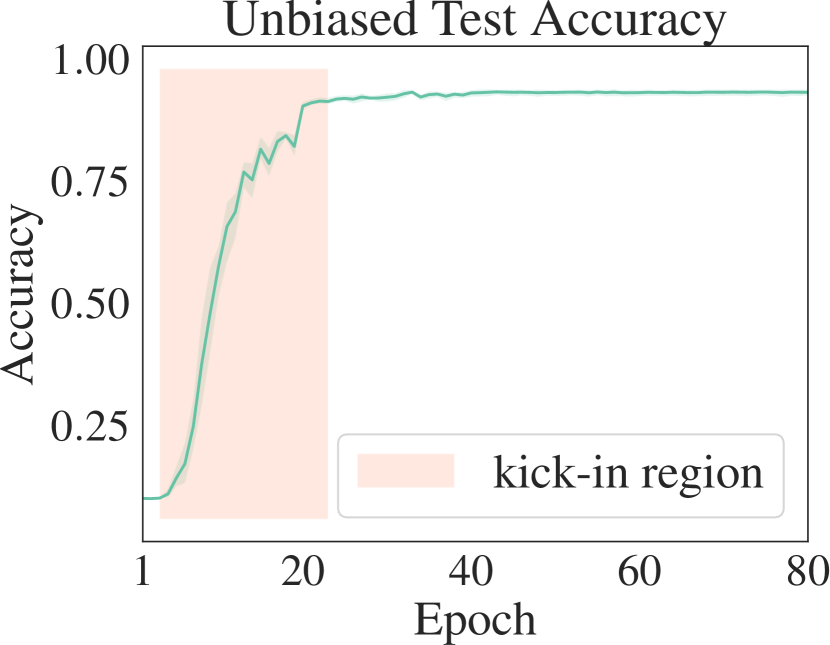
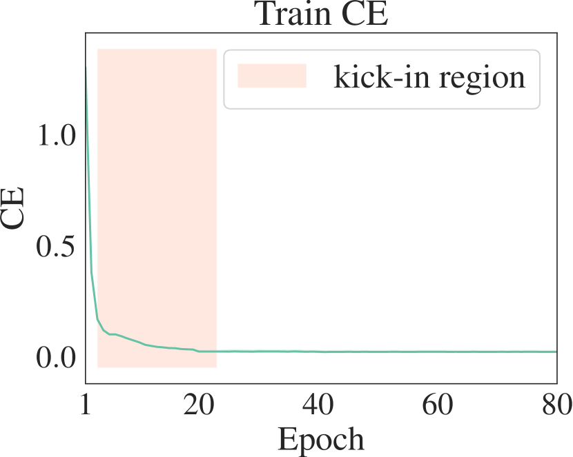
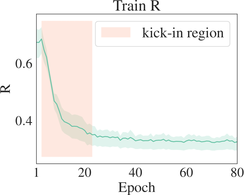
The disentangling term provides a smaller benefit in this case, but, on the other hand, it can always be applied. We find that the ideal case for EnD is when both of the terms can be used in the learning process, leading to better generalization capabilities. Furthermore, we observe a similar pattern in the learning process when employing the full EnD regularization for different values of $\rho$. Figure 5 shows the learning curves for $\rho=0.995$. We notice how models tend to quickly learn the color bias in the first few epochs, as the accuracy on the biased test set is close to 100% (Figure 5(a)). However, once the value of the loss (in this case, we have used the cross-entropy loss, Figure 5(c)) falls below a certain threshold, the contribution $R$ of the EnD term becomes predominant (Figure 5(d)). In this phase, which we call kick-in region, the optimization process begin to rapidly minimize $R$, stopping the model from relying on the bias-related features. This can be observed in the rapid increase of the accuracy on the unbiased test set (Figure 5(b)), whereas the biased accuracy momentarily drops as the models shift their focus from the background color to the digit shape.

4.2 Real world datasets

After benchmarking EnD in a controlled scenario on synthetic data, we move to real world datasets where biases might be subtle and harder to handle. In this section we aim at removing age and gender bias in different datasets. We also apply EnD on a computer-aided diagnosis task, where hidden biases might lead to sub-optimal generalization of the model.

Setup. For CelebA and IMDB Face, we use the ResNet-18 model proposed by He et al. [12]. The network was pre-trained on ImageNet [9], except for the last fully connected layer. The EnD regularization is applied on the average pooling layer, before the fully connected classifier. For CORDA, we use a DenseNet-121 [15] encoder pre-trained on publicly available CXR data, which is then followed by a two-layer fully connected classifier.

4.2.1 CelebA

CelebA [19] is a dataset of for face-recognition tasks, providing 40 attributes for every image. Following Nam et al. [21], we select BlondHair and HeavyMakeup as target attributes $t$ and Male as bias attribute $b$. This choice is dictated by the fact that there is a high correlation between the target and the bias attributes (i.e. most women have blond hair or wear heavy makeup in this dataset). The dataset contains a total of 202,599 images, and following the official train-validation split we obtain 162,770 images for training and 19,867 images for testing our models. Nam et al. [21] build two types of testing dataset: unbiased, by selecting the same number of samples for every possible value of the pair $(t,b)$, and bias-conflicting, by removing from the unbiased set all of the samples where $b$ and $t$ are equal.

		Method	Unbiased	Bias-conflicting
Learn	HairColor	Vanilla	70.25 $\pm$ 0.35	52.52 $\pm$ 0.19
		Group DRO [23]	85.43 $\pm$ 0.53	83.40 $\pm$ 0.67
		LfF[21]	84.24 $\pm$ 0.37	81.24 $\pm$ 1.38
		EnD	91.21 $\pm$ 0.22	87.45 $\pm$ 1.06
Learn	HeavyMakeup	Vanilla	62.00 $\pm$ 0.02	33.75 $\pm$ 0.28
		Group DRO [23]	64.88 $\pm$ 0.42	50.24 $\pm$ 0.68
		LfF[21]	66.20 $\pm$ 1.21	45.48 $\pm$ 4.33
		EnD	75.93 $\pm$ 1.31	53.70 $\pm$ 5.24

Table 3: Performance on CelebA.

Results. Following Nam et al. [21], the accuracy is computed as average accuracy over all the $(t,b)$ pairs. Table 3 shows the results obtained on the CelebA dataset. We observe how the vanilla model heavily relies on the bias attribute, scoring a low accuracy especially on the bias-conflicting sets. EnD, on the other hand, outperforms the baseline in both the tasks. We report reference results [21] of other debiasing algorithms, specifically Group DRO [23] and LfF [21], for comparison with EnD. The results we obtain are significantly higher across most of the evaluation sets, and comparable with Group DRO and LfF on the bias-conflicting set when the target attribute is HeavyMakeup.

4.2.2 IMDB Face

(a)  

(b)  

Figure 6: IMDB train splits: EB1 (a) and EB2 (b).

The IMDB Face dataset [22] contains 460,723 face images annotated with age and gender information. To filter out the misannotated labels of this dataset [22, 30], Kim et al. [16] use a model trained on the Audience benchmark [10], keeping the images where the prediction matches the provided label. Following Kim et al.’s proposed data split, 20% of the IMDB is used as test set, containing samples with age 0-29 or 40+. The remaining data is then split into two extreme-bias subset: EB1 contains women in the age range 0-29 and men with age 40+, while EB2 contains men aged 0-29 and women 40+. Thus, when learning to predict the gender attribute, the bias is given by the age and vice-versa. An example of the EB1 and EB2 training sets is shown in Figure 6.

	Method	Trained on EB1		Trained on EB2
		EB2	Test	EB1	Test
Learn Gender	Vanilla	59.86	84.42	57.84	69.75
	BlindEye [1]	63.74	85.56	57.33	69.90
	Kim et al. [16]	68.00	86.66	64.18	74.50
	EnD	65.49	87.15	69.40	78.19
		$\pm$ 0.81	$\pm$ 0.31	$\pm$ 2.01	$\pm$ 1.18
Learn Age	Vanilla	54.30	77.17	48.91	61.97
	BlindEye [1]	66.80	75.13	64.16	62.40
	Kim et al. [16]	65.27	77.43	62.18	63.04
	EnD	76.04	80.15	74.25	78.80
		$\pm$ 0.25	$\pm$ 0.96	$\pm$ 2.26	$\pm$ 1.48

Table 4: Performance on IMDB Face. When gender is learned, age is the bias, and when age is learned the gender is the bias.

Results. Table 4 shows the results obtained on the IMDB Face dataset. We performed two main experiments: gender and age prediction. Besides the perfomance evaluation on the test set, when training on EB1 we also tested the model’s performance on EB2, and viceversa. This allows us to better evaluate the bias features’ influence on the model prediction. We notice how the baseline model is heavily biased towards age when predicting gender, and towards gender when predicting age. This can be observed on the performance achieved on the EB2 and EB1 sets, both for gender and age prediction. When employing our regularization term, we observe an increase across all of the obtained results: in particular, when training on EB2 for age prediction, we notice an increase from 48.91% to 74.25% on the EB1 set. We also report reference results of other debiasing algorithms, specifically BlindEye [1] and the adversarial approach proposed by Kim et al. [16]. In general, EnD obtains the best results among all the other debiasing algorithms we compared to.

4.2.3 COVID CXR dataset

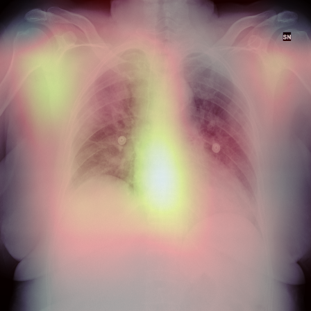
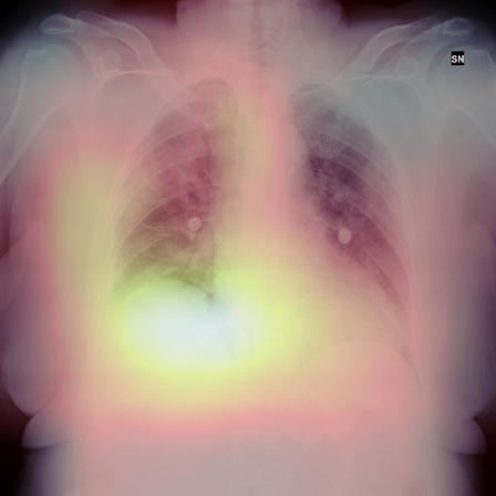
CORDA is a dataset comprising 898 Chest X-Ray images (CXR) that were collected during March and April 2020 by radiology units at Cittá della Salute e della Scienza and San Luigi Gonzaga, in Italy. Virus testing (nasopharingeal swab) was used to determine the presence or absence of COVID-19 infection. The dataset can be split by collecting institution, resulting in CORDA-CDSS with 297 images of COVID-19 positive patients and 150 of negative ones, and CORDA-SLG with 129 positives and 322 negatives. Recent literature [7, 20, 26] shows that merging CXRs coming from different sources poses bias issues, since differences in acquisition techniques given by the scan machines or composition of the population sample might be used by the deep model to distinguish the provenance of the data itself, even when pre-processing techniques are employed. For CORDA, we notice that data coming from Cittá della Salute e della Scienza contain a majority of positive samples, while data coming from San Luigi Gonzaga have a majority of negative samples. Hence, if distinguishing features are embedded in the scans, then the networks might learn to discriminate the source of the data, instead of actually classifying between COVID positives and negatives. To build the test sets, we use 30% of CORDA-CDSS and 30% of CORDA-SLG. The remaining data are then merged and used as training set. Testing on the two distinguished sets allows us to assess whether the prediction of the models are biased towards the origin of the data.

	Test on CORDA-CDSS
	TPR	TNR	BA
Vanilla	69.99 $\pm$ 3.27	59.26 $\pm$ 2.09	64.63 $\pm$ 2.50
EnD	68.16 $\pm$ 2.08	76.30 $\pm$ 2.10	72.22 $\pm$ 0.01
	Test on CORDA-SLG
	TPR	TNR	BA
Vanilla	52.14 $\pm$ 3.20	87.63 $\pm$ 4.37	69.88 $\pm$ 2.95
EnD	68.37 $\pm$ 6.04	84.51 $\pm$ 3.04	75.94 $\pm$ 1.62

Table 5: Performance on CORDA, sorted by collecting institution.

Results. The results obtained on CORDA-CDSS and CORDA-SLG are presented in Table 5. We observe how the vanilla model is in fact biased towards the source of the data. On CORDA-CDSS (which contains mostly positive samples) the vanilla model shows a higher true positive rate (TPR) and a lower true negative rate (TNR). On the other hand, on CORDA-SLG (which contains mostly negative samples) we notice a lower TPR compared to the sensibly higher TNR. Employing EnD helps in improving the results in this case too. While maintaining a similar TPR on CORDA-CDSS and TNR on CORDA-SLG, we obtain an improvement of the TNR 59.26%$\rightarrow$76.30% and of the TPR 52.14%$\rightarrow$68.37% on CORDA-CDSS and CORDA-SLG, respectively. This also results in an increased balanced accuracy (BA) on both of the test sets.

(a)  

(b)  

Figure 7: Grad-CAM on CORDA: vanilla model (a) and EnD-regularized model (b).

As a further insight, we observe in Figure 7(a) that the vanilla model focuses on irrelevant regions outside the lungs area, while the EnD-regularized model mainly focuses on the lower lobes of the lungs (Figure 7(b)).

5 Conclusion

In this work we aimed at EnD-ing the selection of biased features in deep model trained on biased datasets. Towards this end, we have designed a regularizer whose task is to either disentangle deep feature representations with the same bias and to entangle deep features with different biases, but belonging to the same target classification class. Differently from other de-biasing techniques, we do not introduce any additional parameters to be learned and we do not modify the input data: the model itself is naturally driven into choosing deep features which are unbiased, without introducing additional priors to the data. Our experiments show the effectiveness of EnD when compared to other state-of-the-art techniques, excelling in the cases of heavily-biased data (like $\rho=0.999$ for Biased MNIST or IMDB). As an application case, we have also tested the effect of EnD on the COVID diagnosis from CXR images, where the bias is given by the data source and it is not straightforward to detect. In this case we have observed an overall improvement of the performance on the test set as well, showing that our technique may be employed to build more reliable models even in more sensitive tasks.

References

- [1] Mohsan Alvi, Andrew Zisserman, and Christoffer Nellåker. Turning a blind eye: Explicit removal of biases and variation from deep neural network embeddings. In Proceedings of the European Conference on Computer Vision (ECCV), pages 0–0, 2018.
- [2] Ioannis D Apostolopoulos and Tzani A Mpesiana. Covid-19: automatic detection from x-ray images utilizing transfer learning with convolutional neural networks. Physical and Engineering Sciences in Medicine, page 1, 2020.
- [3] Joshua Attenberg, Panos Ipeirotis, and Foster Provost. Beat the machine: Challenging humans to find a predictive model’s “unknown unknowns”. Journal of Data and Information Quality (JDIQ), 6(1):1–17, 2015.
- [4] Hyojin Bahng, Sanghyuk Chun, Sangdoo Yun, Jaegul Choo, and Seong Joon Oh. Learning de-biased representations with biased representations. In International Conference on Machine Learning (ICML), 2020.
- [5] Remi Cadene, Corentin Dancette, Matthieu Cord, Devi Parikh, et al. Rubi: Reducing unimodal biases for visual question answering. In Advances in neural information processing systems, pages 841–852, 2019.
- [6] Christopher Clark, Mark Yatskar, and Luke Zettlemoyer. Don’t take the easy way out: Ensemble based methods for avoiding known dataset biases. In Kentaro Inui, Jing Jiang, Vincent Ng, and Xiaojun Wan, editors, Proceedings of the 2019 Conference on Empirical Methods in Natural Language Processing and the 9th International Joint Conference on Natural Language Processing, EMNLP-IJCNLP 2019, Hong Kong, China, November 3-7, 2019, pages 4067–4080. Association for Computational Linguistics, 2019.
- [7] Beatriz Garcia Santa Cruz, J. Sölter, M. Bossa, and A. Husch. On the composition and limitations of publicly available covid-19 x-ray imaging datasets. ArXiv, abs/2008.11572, 2020.
- [8] Ekin D. Cubuk, Barret Zoph, Dandelion Mane, Vijay Vasudevan, and Quoc V. Le. Autoaugment: Learning augmentation strategies from data. In The IEEE Conference on Computer Vision and Pattern Recognition (CVPR), June 2019.
- [9] J. Deng, W. Dong, R. Socher, L.-J. Li, K. Li, and L. Fei-Fei. ImageNet: A Large-Scale Hierarchical Image Database. In CVPR09, 2009.
- [10] Eran Eidinger, Roee Enbar, and Tal Hassner. Age and gender estimation of unfiltered faces. IEEE Transactions on Information Forensics and Security, 9(12):2170–2179, 2014.
- [11] Abhinav Gupta, Adithyavairavan Murali, Dhiraj Prakashchand Gandhi, and Lerrel Pinto. Robot learning in homes: Improving generalization and reducing dataset bias. In Advances in Neural Information Processing Systems, pages 9094–9104, 2018.
- [12] Kaiming He, Xiangyu Zhang, Shaoqing Ren, and Jian Sun. Deep residual learning for image recognition. In Proceedings of the IEEE conference on computer vision and pattern recognition, pages 770–778, 2016.
- [13] Lisa Anne Hendricks, Kaylee Burns, Kate Saenko, Trevor Darrell, and Anna Rohrbach. Women also snowboard: Overcoming bias in captioning models. In European Conference on Computer Vision, pages 793–811. Springer, 2018.
- [14] European Commission (AI HLEG). Ethics guidelines for trustworthy AI. High-Level Expert Group on Artificial Intelligence, 2019.
- [15] Gao Huang, Zhuang Liu, Laurens Van Der Maaten, and Kilian Q Weinberger. Densely connected convolutional networks. In Proceedings of the IEEE conference on computer vision and pattern recognition, pages 4700–4708, 2017.
- [16] Byungju Kim, Hyunwoo Kim, Kyungsu Kim, Sungjin Kim, and Junmo Kim. Learning not to learn: Training deep neural networks with biased data. In The IEEE Conference on Computer Vision and Pattern Recognition (CVPR), June 2019.
- [17] Sven Laumer, Christian Maier, and Andreas Eckhardt. The impact of business process management and applicant tracking systems on recruiting process performance: an empirical study. Journal of Business Economics, 85(4):421–453, 2015.
- [18] Yann LeCun, Corinna Cortes, and CJ Burges. Mnist handwritten digit database. ATT Labs [Online]. Available: http://yann.lecun.com/exdb/mnist, 2, 2010.
- [19] Ziwei Liu, Ping Luo, Xiaogang Wang, and Xiaoou Tang. Deep learning face attributes in the wild. In Proceedings of International Conference on Computer Vision (ICCV), December 2015.
- [20] Gianluca Maguolo and Loris Nanni. A critic evaluation of methods for covid-19 automatic detection from x-ray images. arXiv preprint arXiv:2004.12823, 2020.
- [21] Junhyun Nam, Hyuntak Cha, Sungsoo Ahn, Jaeho Lee, and Jinwoo Shin. Learning from failure: Training debiased classifier from biased classifier. In Advances in Neural Information Processing Systems, 2020.
- [22] Rasmus Rothe, Radu Timofte, and Luc Van Gool. Deep expectation of real and apparent age from a single image without facial landmarks. International Journal of Computer Vision, 126(2-4):144–157, 2018.
- [23] Shiori Sagawa, Pang Wei Koh, Tatsunori B Hashimoto, and Percy Liang. Distributionally robust neural networks. In International Conference on Learning Representations, 2019.
- [24] Ramprasaath R Selvaraju, Michael Cogswell, Abhishek Das, Ramakrishna Vedantam, Devi Parikh, and Dhruv Batra. Grad-cam: Visual explanations from deep networks via gradient-based localization. In Proceedings of the IEEE international conference on computer vision, pages 618–626, 2017.
- [25] Prabira Kumar Sethy and Santi Kumari Behera. Detection of coronavirus disease (covid-19) based on deep features. Preprints, 2020030300:2020, 2020.
- [26] Enzo Tartaglione, Carlo Alberto Barbano, Claudio Berzovini, Marco Calandri, and Marco Grangetto. Unveiling covid-19 from chest x-ray with deep learning: a hurdles race with small data. Int. J. Environ. Res. Public Health, 17(18):6933, 2020.
- [27] Enzo Tartaglione and Marco Grangetto. Take a ramble into solution spaces for classification problems in neural networks. In International Conference on Image Analysis and Processing, pages 345–355. Springer, 2019.
- [28] Enzo Tartaglione and Marco Grangetto. A non-discriminatory approach to ethical deep learning. In 2020 IEEE 19th International Conference on Trust, Security and Privacy in Computing and Communications (TrustCom), pages 943–950, 2020.
- [29] Tatiana Tommasi, Novi Patricia, Barbara Caputo, and Tinne Tuytelaars. A deeper look at dataset bias. In Domain adaptation in computer vision applications, pages 37–55. Springer, 2017.
- [30] Antonio Torralba, Alexei A Efros, et al. Unbiased look at dataset bias. In CVPR, page 7. Citeseer, 2011.
- [31] Oriol Vinyals, Alexander Toshev, Samy Bengio, and Dumitru Erhan. Show and tell: A neural image caption generator. In Proceedings of the IEEE conference on computer vision and pattern recognition, pages 3156–3164, 2015.
- [32] Haohan Wang, Zexue He, Zachary L. Lipton, and Eric P. Xing. Learning robust representations by projecting superficial statistics out. In International Conference on Learning Representations, 2019.
- [33] Baobao Zhang and Allan Dafoe. Artificial intelligence: American attitudes and trends. Available at SSRN 3312874, 2019.