Online Adversarial Attacks

Abstract

Adversarial attacks expose important vulnerabilities of deep learning models, yet little attention has been paid to settings where data arrives as a stream. In this paper, we formalize the online adversarial attack problem, emphasizing two key elements found in real-world use-cases: attackers must operate under partial knowledge of the target model, and the decisions made by the attacker are irrevocable since they operate on a transient data stream. We first rigorously analyze a deterministic variant of the online threat model by drawing parallels to the well-studied $k$-secretary problem in theoretical computer science and propose Virtual+, a simple yet practical online algorithm. Our main theoretical result shows Virtual+ yields provably the best competitive ratio over all single-threshold algorithms for $k<5$—extending the previous analysis of the $k$-secretary problem. We also introduce the stochastic $k$-secretary—effectively reducing online blackbox transfer attacks to a $k$-secretary problem under noise—and prove theoretical bounds on the performance of Virtual+ adapted to this setting. Finally, we complement our theoretical results by conducting experiments on MNIST, CIFAR-10, and Imagenet classifiers, revealing the necessity of online algorithms in achieving near-optimal performance and also the rich interplay between attack strategies and online attack selection, enabling simple strategies like FGSM to outperform stronger adversaries.

1 Introduction

In adversarial attacks, an attacker seeks to maliciously disrupt the performance of deep learning systems by adding small but often imperceptible noise to otherwise clean data (Szegedy et al., 2014; Goodfellow et al., 2015). Critical to the study of adversarial attacks is specifying the threat model Akhtar & Mian (2018), which outlines the adversarial capabilities of an attacker and the level of information available in crafting attacks. Canonical examples include the whitebox threat model Madry et al. (2017), where the attacker has complete access, and the less permissive blackbox threat model where an attacker only has partial information, like the ability to query the target model (Chen et al., 2017; Ilyas et al., 2019; Papernot et al., 2016).

Previously studied threat models (e.g., whitebox and blackbox) implicitly assume a static setting that permits full access to instances in a target dataset at all times (Tramèr et al., 2018). However, such an assumption is unrealistic in many real-world systems. Countless real-world applications involve streaming data that arrive in an online fashion (e.g., financial markets or real-time sensor networks). Understanding the feasibility of adversarial attacks in this online setting is an essential question.

As a motivating example, consider the case where the adversary launches a man-in-the-middle attack depicted in Fig. 1. Here, data is streamed between two endpoints—i.e., from sensors on an autonomous car to the actual control system. An adversary, in this example, would intercept the sensor data, potentially perturb it, and then send it to the controller. Unlike classical adversarial attacks, such a scenario presents two key challenges that are representative of all online settings.

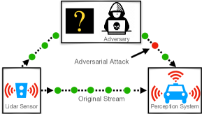
Figure 1: Man-in-the-Middle Attack.

1. Transiency: At every time step, the attacker makes an irrevocable decision on whether to attack, and if she fails, or opts not to attack, then that datapoint is no longer available for further attacks.

2. Online Attack Budget: The adversary—to remain anonymous from stateful defenses —is restricted to a small selection budget and must optimally balance a passive exploration phase before selecting high-value items in the data stream (e.g. easiest to attack) to submit an attack on.

To the best of our knowledge, the only existing approaches that craft adversarial examples on streaming data (Gong et al., 2019a; Lin et al., 2017; Sun et al., 2020) require multiple passes through a data stream and thus cannot be applied in a realistic online setting where an adversary is forced into irrevocable decisions. Moreover, these approaches do not come with theoretical guarantees. Consequently, assessing the practicality of adversarial attacks—to better expose risks—in a truly online setting is still an open problem, and the focus of this paper.

Main Contributions. We formalize the online threat model to study adversarial attacks on streaming data. In our online threat model, the adversary must execute $k$ successful attacks within $n$ streamed data points, where $k\ll n$. As a starting point for our analysis, we study the deterministic online threat model in which the actual value of an input—i.e., the likelihood of a successful attack—is revealed along with the input. Our first insight elucidates that such a threat model, modulo the attack strategy, equates to the $k$-secretary problem known in the field of optimal stopping theory Dynkin (1963); Kleinberg (2005), allowing for the application of established online algorithms for picking optimal data points to attack. We then propose a novel online algorithm Virtual+ that is both practical, simple to implement for any pair $(k,n)$, and requires no additional hyperparameters.

Besides, motivated by attacking blackbox target models, we also introduce a modified secretary problem dubbed the stochastic $k$-secretary problem, which assumes the values an attacker observes are stochastic estimates of the actual value. We prove theoretical bounds on the competitive ratio—under mild feasibility assumptions—for Virtual+in this setting. Guided by our theoretical results, we conduct a suite of experiments on both toy and standard datasets and classifiers (i.e., MNIST, CIFAR-10, and Imagenet). Our empirical investigations reveal two counter-intuitive phenomena that are unique to the online blackbox transfer attack setting: 1.) In certain cases attacking robust models may in fact be easier than non-robust models based on the distribution of values observed by an online algorithm. 2.) Simple attackers like FGSM can seemingly achieve higher online attack transfer rates than stronger PGD-attackers when paired with an online algorithm, demonstrating the importance of carefully selecting which data points to attack. We summarize our key contributions:

• We formalize the online adversarial attack threat model as an online decision problem and rigorously connect it to a generalization of the k-secretary problem.

• We introduce and analyze Virtual+, an extension of Virtual for the $k$-secretary problem yielding a significant practical improvement ($60\%$).

  We then provide, via novel techniques, a tractable formula for its competitive ratio, partially answering one of Albers & Ladewig (2020)’s open questions (see footnote 1) and achieving a new state-of-the-art competitive ratio for $k<5$.

• We propose Alg. 2 that leverages (secretary) online algorithms to perform efficient online adversarial attacks. We compare different online algorithms including Virtual+ on MNIST, CIFAR-10, and Imagenet in the challenging Non-Interactive BlackBox transfer (NoBox) setting.

2 Background and Preliminaries

Classical Adversarial Attack Setup. We are interested in constructing adversarial examples against some fixed target classifier $f_{t}:\mathcal{X}\to\mathcal{Y}$ which consumes input data points $x\in\mathcal{X}$ and labels them with a class label $y\in\mathcal{Y}$. The goal of an adversarial attack is then to produce an adversarial example $x^{\prime}\in\mathcal{X}$, such that $f_{t}(x^{\prime})\neq y$, and where the distance $d(x,x^{\prime})\leq\gamma$. Then, equipped with a loss $\ell$ used to evaluate $f_{t}$, an attack is said to be optimal if (Carlini & Wagner, 2017; Madry et al., 2017),

$$\textstyle x^{\prime}\in\operatorname*{\arg\!\max}_{x^{\prime}\in{\mathcal{X}}}\ell(f_{t}(x^{\prime}),y)\,,\;\;\text{s.t.}\;\;d(x,x^{\prime})\leq\gamma\,.$$ (1)

Note that the formulation above makes no assumptions about access and resource restrictions imposed upon the adversary. Indeed, if the parameters of $f_{t}$ are readily available, we arrive at the familiar whitebox setting, and problem in Eq. 1 is solved by following the gradient $\nabla_{x}f_{t}$ that maximizes $\ell$.

k-Secretary Problem. The secretary problem is a well-known problem in theoretical computer science Dynkin (1963); Ferguson et al. (1989). Suppose that we are tasked with hiring a secretary from a randomly ordered set of $n$ potential candidates to select the secretary with maximum value. The secretaries are interviewed sequentially and reveal their actual value on arrival. Thus, the decision to accept or reject a secretary must be made immediately, irrevocably, and without knowledge of future candidates. While there exist many generalizations of this problem, in this work, we consider one of the most canonical generalizations known as the $k$-secretary problem Kleinberg (2005). Here, instead of choosing the best secretary, we are tasked with choosing $k$ candidates to maximize the expected sum of values. Typically, online algorithms that attempt to solve secretary problems are evaluated using the competitive ratio, which is the value of the objective achieved by an online algorithm compared to an optimal value of the objective that is achieved by an ideal “offline algorithm,” i.e., an algorithm with access to the entire candidate set. Formally, an online algorithm $\mathcal{A}$ that selects a subset of items $S_{\mathcal{A}}$ is said to be $C$-competitive to the optimal algorithm OPT which greedily selects a subset of items $S^{*}$ while having full knowledge of all $n$ items, if asymptotically in $n$

$$\mathbb{E}_{\pi\sim\mathcal{S}_{n}}[\mathbb{V}(S_{\mathcal{A}})]\geq(C+o(1))\mathbb{V}(S^{*})\,,$$ (2)

where $\mathbb{V}$ is a set-value function that determines the sum utility of each algorithm’s selection, and the expectations are over permutations sampled from the symmetric group of $n$ elements, $\mathcal{S}_{n}$, acting on the data. In §4, we shall further generalize the $k$-secretary problem to its stochastic variant where the online algorithm is no longer privy to the actual values but must instead choose under uncertainty.

3 Online Adversarial Attacks

Motivated by our more realistic threat model, we now consider a novel adversarial attack setting where the data is no longer static but arrives in an online fashion.

3.1 Adversarial Attacks as Secretary Problems

The defining feature of the online threat model—in addition to streaming data and the fact that we may not have access to the target model $f_{t}$—is the online attack budget constraint. Choosing when to attack under a fixed budget in the online setting can be related to a secretary problem. We formalize this online adversarial attack problem in the boxed online threat model below.

In the online threat model we are given a data stream $\mathcal{D}=\{(x_{1},y_{1}),\ldots,(x_{n},y_{n})\}$ of $n$ samples ordered by their time of arrival. In order to craft an attack against the target model $f_{t}$, the adversary selects, using its online algorithm $\mathcal{A}$, a subset $S_{\mathcal{A}}\subset\mathcal{D}$ of items to maximize:

$$\mathbb{V}(S_{\mathcal{A}})\!:=\!\!\!\sum_{(x,y)\in S_{\mathcal{A}}}\ell(f_{t}(\textsc{Att}(x)),y)\ \text{ s.t. }|S_{A}|\leq k,$$ (3)

where $\textsc{Att}(x)$ denotes an attack on $x$ crafted by a fixed attack method Att that might or might not depend on $f_{t}$. From now on we define $x_{i}^{\prime}=\textsc{Att}(x_{i})$. Intuitively, the adversary chooses $k$ instances that are the “easiest" to attack, i.e. samples with the highest value. Note that selecting an instance to attack does not guarantee a successful attack. Indeed, a successful attack vector may not exist if the perturbation budget $\gamma$ is too small. However, stating the adversarial goal as maximizing the value of $S_{\mathcal{A}}$ leads to the measurable objective of calculating the ratio of successful attacks in $S_{\mathcal{A}}$ versus $S^{*}$.

If the adversary knows the true value of a datapoint then the online attack problem reduces to the original $k$-secretary. On the other hand, the adversary might not have access to $f_{t}$, and instead, the adversary’s value function may be an estimate of the true value—e.g.,  the loss of a surrogate classifier, and the adversary must make selection decisions in the face of uncertainty. The theory developed in this paper will tackle both the case where values $v_{i}:=\ell(f_{t}(x_{i}^{\prime}),y_{i})$ for $i\in\{1,\ldots,n\}:=[n]$ are known (§3.2), as well as the richer stochastic setting with only estimates of $v_{i}\,,\,i\in[n]$ (§4).

Practicality of the Online Threat Model. It is tempting to consider whether in practice the adversary should forego the online attack budget and instead attack every instance. However, such a strategy poses several critical problems when operating in real-world online attack scenarios. Chiefly, attacking any instance in $\mathcal{D}$ incurs a non-trivial risk that the adversary is detected by a defense mechanism. Indeed, when faced with stateful defense strategies (e.g. Chen et al. (2020)), every additional attacked instance further increases the risk of being detected and rendering future attacks impotent. Moreover, attacking every instance may be infeasible computationally for large $n$ or impractical based on other real-world constraints. Generally speaking, as conventional adversarial attacks operate by restricting the perturbation to a fraction of the maximum possible change (e.g., $\ell_{\infty}$-attacks), online attacks analogously restrict the time window to a fraction of possible instances to attack. Similarly, knowledge of $n$ is also a factor that the adversary can easily control in practice. For example, in the autonomous control system example, the adversary can choose to be active for a short interval—e.g., when the autonomous car is at a particular geospatial location—and thus set the value for $n$.

Online Threat Model.

The online threat model relies on the following key definitions: • The target model $f_{t}$. The adversarial goal is to attack some target model $f_{t}:\mathcal{X}\rightarrow\mathcal{Y}$, through adversarial examples that respect a chosen distance function, $d$, with tolerance $\gamma$. • The data stream $\mathcal{D}$. The data stream $\mathcal{D}$ contains the $n$ examples $(x_{i},y_{i})$ ordered by their time of arrival. At any timestep $i$, the adversary receives the corresponding item in $\mathcal{D}$ and must decide whether to execute an attack or forever forego the chance to attack this item. • Online attack budget $k$. The adversary is limited to a maximum of $k$ attempts to craft attacks within the online setting, thus imposing that each attack is on a unique item in $\mathcal{D}$. • A value function $\mathcal{V}$. Each item in the dataset is assigned a value on arrival by the value function $\mathcal{V}:\mathcal{X}\times\mathcal{Y}\rightarrow\mathbb{R}_{+}$ which represents the utility of selecting the item to craft an attack. This can be the likelihood of a successful attack under $f_{t}$ (true value) or a stochastic estimate of the incurred loss given by a surrogate model $f_{s}\approx f_{t}$. The online threat model corresponds to the setting where the adversary seeks to craft adversarial attacks (i) against a target model $f_{t}\in{\mathcal{F}}$, (ii) by observing items in $\mathcal{D}$ that arrive online, (iii) and choosing $k$ optimal items to attack by relying on (iv) an available value function $\mathcal{V}$. The adversary’s objective is then to use its value function towards selecting items in $\mathcal{D}$ that maximize the sum total value of selections $\mathbb{V}$ (Eq. 3).

3.2 Virtual+ for Adversarial Secretary Problems

Let us first consider the deterministic variant of the online threat model, where the true value is known on arrival. For example consider the value function $\mathcal{V}(x_{i},y_{i})=\ell(f_{t}(x^{\prime}_{i}),y_{i})=v_{i}$ i.e. the loss resulting from the adversary corrupting incoming data $x_{i}$ into $x^{\prime}_{i}$. Under a fixed attack strategy, the selection of high-value items from $\mathcal{D}$ is exactly the original $k$-secretary problem and thus the adversary may employ any $\mathcal{A}$ that solves the original $k$-secretary problem.

Well-known single threshold-based algorithms that solve the $k$-secretary problem include the Virtual, Optimistic Babaioff et al. (2007) and the recent Single-Ref algorithm Albers & Ladewig (2020). In a nutshell, these online algorithm consists of two phases—a sampling phase followed by a selection phase—and an optimal stopping point $t$ (threshold) that is used by the algorithm to transition between the phases. In the sampling phase, the algorithms passively observe all data points up to a pre-specified threshold $t$. Note that $t$ itself is algorithm-specific and can be chosen by solving a separate optimization problem. Additionally, each algorithm also maintains a sorted reference list $R$ containing the top-$k$ elements. Each algorithm then executes the selection phase through comparisons of incoming items to those in $R$ and possibly updating $R$ itself in the process (see §D).

Indeed, the simple structure of both the Virtual and Optimistic algorithms—e.g., having few hyperparameters and not requiring the algorithm to involve Linear Program’s for varying values of $n$ and $k$—in addition to being $(1/e)$-competitive (optimal for $k=1$) make them suitable candidates for solving Eq. 3. However, the competitive ratio of both algorithms in the small $k$ regime—but not $k=1$—has shown to be sub-optimal with Single-Ref provably yielding larger competitive ratios at the cost of an additional hyperparameter selected via combinatorial optimization when $n\to\infty$.

We now present a novel online algorithm, Virtual+, that retains the simple structure of Virtual and Optimistic, with no extra hyperparameters, but leads to a new state-of-the-art competitive ratio for $k<5$. Our key insight is derived from re-examining the selection condition in the Virtual algorithm and noticing that it is overly conservative and can be simplified. The Virtual+ algorithm is presented in Algorithm 1, where the removed condition in Virtual (L2-3) is in pink strikethrough. Concretely, the condition that is used by Virtual but not by Virtual+ updates $R$ during the selection phase without actually picking the item as part of $S_{\mathcal{A}}$. Essentially, this condition is theoretically convenient and leads to a simpler analysis by ensuring that the Virtual algorithm never exceeds $k$ selections in $S_{\mathcal{A}}$. Virtual+ removes this conservative $R$ update criteria in favor of a simple to implement condition, $|S_{\mathcal{A}}|\leq k$ line 4 (in pink). Furthermore, the new selection rule also retains the simplicity of Virtual leading to a painless application to online attack problems.

Inputs: $t\in[k\dots n-k]$, $R=\emptyset$, $S_{\mathcal{A}}=\emptyset$
Sampling phase: Observe the first $t$ data points and construct a sorted list $R$ with the indices of the top $k$ data points seen. The method sort ensures: $\mathcal{V}(R[1])\geq\mathcal{V}(R[2])\dots\geq\mathcal{V}(R[k]).$
Selection phase: {//Virt+ removes L2-3 and adds L4 }

1:  for $i:=t+1$ to $n$  do

2:     if $\mathcal{V}(i)\geq\mathcal{V}(R[k])$ and $R[k]>t$ then

3:        $R$ = $\texttt{sort}(R\cup\{i\}\setminus\{R[k]\})$

4:     else if $\mathcal{V}(i)\geq\mathcal{V}(R[k])$ and $|S_{\mathcal{A}}|\leq k$  then

5:        $R$ = $\texttt{sort}(R\cup\{i\}\setminus\{R[k]\})$ {// Update $R$}

6:        $S_{\mathcal{A}}=S_{\mathcal{A}}\cup\{i\}$ {// Select element $i$}

Algorithm 1 Virtual and Virtual+ 

Figure 2: Virtual+ observes $v_{i}$ (or estimates) and maintains $R$ during the sampling phase. Items are then picked into $S_{\mathcal{A}}$, after threshold $t$,

Competitive ratio of Virtual+. What appears to be a minor modification in Virtual+ compared to Virtual leads to a significantly more involved analysis but a larger competitive ratio. In Theorem 1, we derive the analytic expression that is a tight lower bound for the competitive ratio of Virtual+ for general-$k$. We see that Virtual+ provably improves in competitive ratio for $k<5$ over both Virtual, Optimistic, and in particular the previous best single threshold algorithm, Single-Ref.

Theorem 1.

The competitive ratio of Virtual+ for $k\geq 2$ with threshold $t_{k}=\alpha n$ can asymptotically be lower bounded by the following concave optimization problem,

$$C_{k}\geq\max_{\alpha\in[0,1]}f(\alpha):={\alpha}^{k}\sum_{m=0}^{k-1}a_{m}\ln^{m}(\alpha)-\alpha a_{0}\quad where\quad a_{m}:=\big{(}\tfrac{k^{k}}{(k-1)^{k-m}}-k^{m}\big{)}\frac{(-1)^{m+1}}{m!}\,.$$ (4)

Particularly, we get $C_{2}\geq 0.427,C_{3}\geq.457,C_{4}\geq.4769$ outperforming Albers & Ladewig (2020).

Connection to Prior Work. The full proof for Theorem 1 can be found in §B along with a simple but illustrative proof for $k=2$ in §A. Theorem 1 gives a tractable way to compute the competitive ratio of Virtual+ for any $k$, that improve the previous state-of-the-art (Albers & Ladewig, 2020) in terms of single threshold $k$-secretary algorithms for $k<5$ and $k>100$. However, it is also important to contextualize Virtual+ against recent theoretical advances in this space. Most prominently, Buchbinder et al. (2014) proved that the $k$-secretary problem can be solved optimally (in terms of competitive ratio) using linear programs (LPs), assuming a fixed length of $n$. But these optimal algorithms are typically not feasible in practice. Critically, they require individually tuning multiple thresholds by solving a separate LP with $\Omega(nk^{2})$ parameters for each length of the data stream $n$, and the number of constraints grows to infinity as $n\rightarrow\infty$. Chan et al. (2014) showed that optimal algorithms with $k^{2}$ thresholds could be obtained using infinite LPs and derived an optimal algorithm for $k=2$ Nevertheless they require a large number of parameters and the scalability of infinite LPs for $k>2$ remains uncertain. In this work, we focus on practical methods with a single threshold (i.e., with $O(1)$ parameters, e.g. Algorithm 1) that do not require involved computations that grow with $n$.

Open Questions for Single Threshold Secretary Algorithms. Albers & Ladewig (2020) proposed new non-asymptotic results on the $k$-secretary problem that outperform asymptotically optimal algorithms—opening a new range of open questions for the $k$-secretary problem. While this problem is considered solved when working with probabilistic algorithms with $\Theta(nK^{2})$ parameters (Buchbinder et al., 2014), finding optimal non-asymptotic single-threshold ($O(1)$ parameters) algorithms is still an open question. As a step towards answering this question, our work proposes a practical algorithm that improves upon Albers & Ladewig (2020) for $k=2,\ldots,4$ with an optimal threshold that can be computed easily as it has a closed form.

4 Stochastic Secretary Problem

In practice, online adversaries are unlikely to have access to the target model $f_{t}$. Instead, it is reasonable to assume that they have partial knowledge.

Following Papernot et al. (2017); Bose et al. (2020) we focus on modeling that partial knowledge by equipping the adversary with a surrogate model or representative classifier $f_{s}$. Using $f_{s}$ as opposed to $f_{t}$ means that we can compute the value $\mathcal{V}_{i}:=\ell(f_{s}(x_{i}^{\prime}),y_{i})$ of an incoming data point. This value $\mathcal{V}_{i}$ acts as an estimate of the value of interest $v_{i}:=\ell(f_{t}(x_{i}^{\prime}),y_{i})$. The stochastic $k$-secretary problem is then to pick, under the noise model induced by using $f_{s}$, the optimal subset $S_{\mathcal{A}}$ of size $k$ from $\mathcal{D}$. Thus, with no further assumptions on $f_{s}$ it is unclear whether online algorithms, as defined in  §3.2, are still serviceable under uncertainty.

Sources of randomness. Our method relies on the idea that we can use the surrogate model $f_{s}$ to estimate the value of some adversarial examples on the target model $f_{t}$. We justify here how partial knowledge on $f_{t}$ could provide us an estimate of $v_{i}$. For example, we may know the general architecture and training procedure of $f_{t}$, but there will be inherent randomness in the optimization (e.g., due to initialization or data sampling), making it impossible to perfectly replicate $f_{t}$.

Moreover, it has been observed that, in practice, adversarial examples transfer across models (Papernot et al., 2016; Tramèr et al., 2017). In that context, it is reasonable to assume that the random variable $\mathcal{V}_{i}:=\ell(f_{s}(x^{\prime}_{i}),y_{i})$ is likely to be close to $v_{i}:=\ell(f_{t}(x^{\prime}_{i}),y_{i})$. We formalize this idea in Assumption 1

4.1 Stochastic Secretary Algorithms

In the stochastic $k$-secretary problem, we assume access to random variables $\mathcal{V}_{i}$ and that $v_{i}$ are fixed for $i=1,\ldots,n$ and the goal is to maximize a notion of stochastic competitive ratio. This notion is similar to the standard competitive ratio defined in Eq. 2 with a minor difference that in the stochastic case, the algorithm does not have access to the values $v_{i}$ but to $\mathcal{V}_{i}$ that is an estimate of $v_{i}$. An algorithm is said to be $C_{s}$-competitive in the stochastic setting if asymptotically in $n$,

$$\mathbb{E}_{\pi\sim\mathcal{S}_{n}}[\mathbb{V}(S_{\mathcal{A}})]\geq(C_{s}+o(1))\mathbb{V}(S^{*})\,.$$

Here the expectation is taken over $\mathcal{S}_{n}$ (uniformly random permutations of the datastream $\mathcal{D}$ of size $n$) and over the randomness of $\mathcal{V}_{i}\,,\,i=1,\ldots,n$. $S_{\mathcal{A}}$ and $S^{*}$ are the set of items chosen by the stochastic online and offline algorithms respectively (note that while the online algorithm has access to $\mathcal{V}_{i}$, the offline algorithm picks the best $v_{i}$) and $\mathbb{V}$ is a set-value function as defined previously.

Analysis of algorithms. In the stochastic setting, all online algorithms observe $\mathcal{V}_{i}$ that is an estimate of the actual value $v_{i}$. Since the goal of the algorithm is to select the $k$-largest values by only observing random variables $(\mathcal{V}_{i})$ it is requisite to make a feasibility assumption on the relationship between values $v_{i}$ and $\mathcal{V}_{i}$. Let us denote $\operatorname*{top_{k}}\{v_{i}\}$ as the set of top-$k$ values among $(v_{i})$.

Assumption 1 (Feasibility).

$\exists\gamma>0$ such that ${\mathbb{P}}[\mathcal{V}_{i}\in\operatorname*{top_{k}}\{\mathcal{V}_{i}\}\,|\,v_{i}\in\operatorname*{top_{k}}\{v_{i}\}]\geq\gamma,\,\forall n\geq 0$.

Assumption 1 is a feasibility assumption as if the ordering of $(\mathcal{V}_{i})$ does not correspond at all with the ordering of $(v_{i})$ then there is no hope any algorithm—online or an offline oracle—would perform better than random when picking $k$ largest $v_{i}$ by only observing $(\mathcal{V}_{i})$. In the context of adversarial attacks, such an assumption is quite reasonable as in practice there is strong empirical evidence between the transfer of adversarial examples between surrogate and target models (see §C.1, for the empirical caliber of assumption 1). We can bound the competitive ratio in the stochastic setting.

Theorem 2.

Let us assume that Virtual+ observes independent random variables $\mathcal{V}_{i}$ following Assumption 1. Its stochastic competitive ratio $C_{s}$ can be bounded as follows,

$$C\geq C_{s}\geq\gamma C$$ (5)

The proof of Thm. 2 can be found in §C. Such a theoretical result is quite interesting as the stochastic setting initially appears significantly more challenging due to the non-zero probability that the observed ordering of historical values, $\mathcal{V}_{i}$, not being faithful to the true ranking based on $v_{i}$.

4.2 Results on Synthetic Data

We assess the performance of classical single threshold online algorithms and Virtual+ in solving the stochastic $k$-secretary problem on a synthetic dataset of size $n=100$ with $k\in[1,10]$. The value of a data point is its index in $\mathcal{D}$ prior to applying any permutation $\pi\sim\mathcal{S}_{n}$ plus noise $\mathcal{N}(0,\sigma^{2})$. We compute and plot the competitive ratio over $10k$ unique permutations of each algorithm in Figure 3.

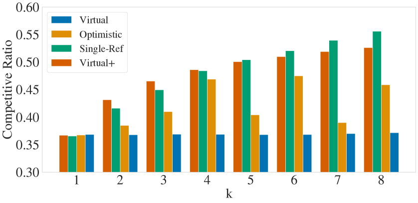
Figure 3: Estimation of the competitive ratio of online algorithms in the stochastic $k$-secretary problem with $\sigma^{2}=10$.

Inputs: Permuted Datastream: $\mathcal{D}_{\pi}$, Online Algorithm: $\mathcal{A}$, Surrogate classifier: $f_{s}$, Target classifier: $f_{t}$, Attack method: Att, Loss: $\ell$, Budget: $k$, Online Fool rate: $F^{\mathcal{A}}_{\pi}=0$.

1:  for $(x_{i},y_{i})$ in $\mathcal{D}_{\pi}$ do

2:     $x_{i}^{\prime}\leftarrow\textsc{Att}(x_{i})$ {// Compute the attack}

3:     $\mathcal{V}_{i}\leftarrow\ell(f_{s}(x_{i}^{\prime}),y_{i})$ {// Estimate $v_{i}$}

4:     if $\mathcal{A}(\mathcal{V}_{1},\ldots,\mathcal{V}_{i},k)==\textsc{True}$ then

5:        $F^{\mathcal{A}}_{\pi}\leftarrow F^{\mathcal{A}}_{\pi}+\tfrac{\mathbf{1}\{f_{t}(x_{i}^{\prime})\neq y_{i}\}}{k}$ {// Submit $x_{i}^{\prime}$}

6:  return: $F^{\mathcal{A}}_{\pi}$ {//$\mathcal{A}$ always submits $k$ attacks}

Algorithm 2 Online Adversarial Attack

As illustrated for $k=1$ all algorithms achieve the optimal $(1/e)$-deterministic competitive ratio in the stochastic setting. Note that the noise level, $\sigma^{2}$, appears to have a small impact on the performance of the algorithms (§E.2). This substantiates our result in Thm. 2 indicating that $C_{n}$-competitive algorithms only degrade by a small factor in the stochastic setting. For $k<5$, Virtual+ achieves the best competitive ratio—empirically validating Thm 1—after which Single-Ref is superior.

5 Experiments

We investigate the feasibility of online adversarial attacks by considering an online version of the challenging NoBox setting (Bose et al., 2020) in which the adversary must generate attacks without any access, including queries, to the target model $f_{t}$. Instead, the adversary only has access to a surrogate $f_{s}$ which is similar to $f_{t}$. In particular, we pick at random a $f_{t}$ and $f_{s}$ from an ensemble of pre-trained models from various canonical architectures. We perform experiments on the MNIST LeCun & Cortes (2010) and CIFAR-10 Krizhevsky (2009) datasets where we simulate a $\mathcal{D}$ by generating $1000$ permutations of the test set and feeding each instantiation to Alg. 2. In practice, online adversaries compute the value $\mathcal{V}_{i}=\ell(f_{s}(x^{\prime}_{i}),y_{i})$ of each data point in $\mathcal{D}$ by attacking $f_{s}$ using their fixed attack strategy (where $\ell$ is the cross-entropy), but the decision to submit the attack to $f_{t}$ is done using an online algorithm $\mathcal{A}$ (see Alg. 2). As representative attack strategies, we use the well-known FGSM attack (Goodfellow et al., 2015) and a universal whitebox attack in PGD (Madry et al., 2017). We are most interested in evaluating the online fool rate, which is simply the ratio of successfully executed attacks against $f_{t}$ out of a possible of $k$ attacks selected by $\mathcal{A}$. The architectures used for $f_{s}$, $f_{t}$, and additional metrics (e.g. competitive ratios) can be found in §E .

Baselines. We rely on two main baselines, first we use a naive baseline–a lower bound–where the data points are picked uniformly at random, and an upper bound with the OPT baseline where attacks, while crafted using $f_{s}$, are submitted by using the true value $v_{i}$ and thus utilizing $f_{t}$.

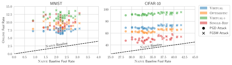
Figure 4: Plot of online fool rates for $k=1000$ against PGD-robust models using different online algorithms $\mathcal{A}$, attacks, datasets, and $20$ different permutations. For a given $x$-coordinate, a higher $y$-coordinate is better.

Q1: Utility of using an online algorithm. We first investigate the utility of using an online algorithm, $\mathcal{A}$, in selecting data points to attack in comparison to the Naive baseline. For a given permutation $\pi$ and an attack method (FGSM or PGD), we compute the online fool rate of the Naive baseline and an $\mathcal{A}$ as $F^{\textsc{Naive}}_{\pi}$, $F^{\mathcal{A}}_{\pi}$ respectively. In Fig. 4, we uniformly sample $20$ permutations $\pi_{i}\sim\mathcal{S}_{n},\,i\in[n],$ of $\mathcal{D}$ and plot a scatter graph of points with coordinates $(F^{\textsc{Naive}}_{\pi_{i}},F^{\mathcal{A}}_{\pi_{i}})$, for different $\mathcal{A}$’s, attacks with $k=1000$, and datasets. The line $y=x$ corresponds to the Naive baseline performance —i.e. coordinates $(F^{\textsc{Naive}}_{\pi},F^{\textsc{Naive}}_{\pi})$—and each point above that line corresponds to an $\mathcal{A}$ that outperforms the baseline on a given $\pi_{i}$. As observed, all $\mathcal{A}$’s significantly outperform the Naive baseline with an average aggregate improvement of 7.5% and 34.1% on MNIST and CIFAR-10.

		MNIST (Online fool rate in %)			CIFAR-10 (Online fool rate in %)			Imagenet (Online fool rate in %)
	Algorithm	​$k=10$​	​$k=10^{2}$​	​$k=10^{3}$​	​$k=10$​	​$k=10^{2}$​	​$k=10^{3}$​	​$k=10$​	​$k=10^{2}$​	​$k=10^{3}$​
FGSM	Naive	64.1	47.8	45.7	60.7	59.2	59.2	66.0	66.3	65.0
	Opt	87.0	84.7	83.6	86.6	87.3	86.5	98.7	95.3	96.2
	Optimistic	79.0	77.6	75.3	75.3	72.8	71.9	86.0	80.4	79.9
	Virtual	78.6	79.1	77.4	76.1	77.1	75.4	85.3	84.9	84.3
	Single-Ref	85.1	83.0∗	72.3	80.4	84.0	66.0	94.0∗	92.4∗	72.5
	Virtual+	80.4	82.5∗	82.9	82.9	86.3	85.2	96.0∗	95.0∗	95.8
PGD	Naive	69.7	67.2	67.9	72.5	70.4	68.6	72.5	72.5	73.8
	Opt	73.6	49.8	49.6	83.7	80.6	79.9	82.5	80.2	76.8
	Optimistic	66.2	48.2	45.1	79.1	76.6	76.0	87.5∗	78.0∗	74.5∗
	Virtual	63.4	46.2	46.8	78.3	77.5	76.9	80.0∗	74.0∗	75.6∗
	Single-Ref	71.5	49.7∗	42.9	80.2∗	79.6∗	74.5	77.5∗	79.5∗	75.2∗
	Virtual+	68.2	49.3∗	49.7	81.2∗	80.1∗	79.5	77.5∗	79.0∗	76.4∗

Table 1: Online fool rate of various online algorithms on non-robust models. For a given attack and value of $k$: $\mathbf{\bullet}$ at least 97%, $\mathbf{\bullet}$ at least 95%, $\mathbf{\bullet}$ at least 90%, $\mathbf{\bullet}$ less than 90% of the optimal performance. ^∗ indicates when there is several best methods with overlapping error bars. Detailed results with error bars can be found in §E.1.

Q2: Online Attacks on Non-Robust Classifiers. We now conduct experiments on non-robust MNIST, CIFAR-10, and Imagenet classifiers. We report the average performance of all online algorithms, and the optimal offline algorithm Opt in Tab. 5. For MNIST, we find that the two best online algorithms are Single-Ref and our proposed Virtual+ which approach the upper bound provided by Opt. For experiments with $k<5$ please see §E.5. For $k=10$ and $k=100$, Single-Ref is slightly superior while for $k=1000$ Virtual+ is the best method with an average relative improvement of $15.3\%$. This is unsurprising as Virtual+ does not have any additional hyperparameters unlike Single-Ref which appears more sensitive to the choice of optimal thresholds and reference ranks, both of which are unknown beyond $k=100$ and non-trivial to find in closed form (see §E.3 for details). On CIFAR-10, we observe that Virtual+ is the best approach regardless of attack strategy and the online attack budget $k$. Finally, for ImageNet we find that all online algorithms improve over the Naive baseline and approach saturation to the optimal offline algorithm, and as a result, all algorithms are equally performant—i.e. within error bars (see §E.1 for more details). A notable observation is that even conventional whitebox adversaries like FGSM and PGD become strong blackbox transfer attack strategies when using an appropriate $\mathcal{A}$.

		MNIST (Online fool rate in %)			CIFAR-10 (Online fool rate in %)
	Algorithm	$k=10$	$k=100$	$k=1000$	$k=10$	$k=100$	$k=1000$
FGSM	Naive	$2.1\pm 4.5$	$2.1\pm 1.4$	$2.1\pm 0.4$	31.9 $\pm$ 14.2	32.6 $\pm$ 4.7	32.5 $\pm$ 1.5
	Opt	80.0 $\pm$ 0.0	55.0 $\pm$ 0.0	18.9 $\pm$ 0.0	100.0 $\pm$ 0.0	100.0 $\pm$ 0.0	97.2 $\pm$ 0.0
	Optimistic	$49.7\pm 0.6$	$25.7$ $\pm$ $0.1$	$9.7$ $\pm$ $0.0$	72.4 $\pm$ 0.5	64.6 $\pm$ 0.1	61.9 $\pm$ 0.0
	Virtual	49.8 $\pm$ 0.5	27.8 $\pm$ 0.1	8.1 $\pm$ 0.0	75.1 $\pm$ 0.5	74.3 $\pm$ 0.1	68.9 $\pm$ 0.0
	Single-Ref	62.0 $\pm$ 0.7	45.2 $\pm$ 0.2	10.2 $\pm$ 0.0	84.3 $\pm$ 0.6	90.9 $\pm$ 0.3	48.6 $\pm$ 0.1
	Virtual+	68.2 $\pm$ 0.5	42.2 $\pm$ 0.1	12.7 $\pm$ 0.0	91.5 $\pm$ 0.4	96.5 $\pm$ 0.1	91.7 $\pm$ 0.0
PGD	Naive	1.8 $\pm$ 4.1	1.9 $\pm$ 1.4	1.9 $\pm$ 0.4	39.1 $\pm$ 14.2	38.9 $\pm$ 4.4	38.7 $\pm$ 1.5
	Opt	58.9 $\pm$ 0.4	39.9 $\pm$ 0.1	16.1 $\pm$ 0.0	100.0 $\pm$ 0.0	100.0 $\pm$ 0.0	98.0 $\pm$ 0.0
	Optimistic	34.9 $\pm$ 0.5	19.2 $\pm$ 0.1	8.2 $\pm$ 0.0	75.4 $\pm$ 1.9	68.5 $\pm$ 0.4	66.0 $\pm$ 0.1
	Virtual	35.4 $\pm$ 0.5	21.8 $\pm$ 0.1	7.2 $\pm$ 0.0	78.1 $\pm$ 1.7	77.3 $\pm$ 0.5	72.8 $\pm$ 0.1
	Single-Ref	44.1 $\pm$ 0.6	33.9 $\pm$ 0.2	8.3 $\pm$ 0.0	86.2 $\pm$ 2.2	91.9 $\pm$ 0.9	53.2 $\pm$ 0.3
	Virtual+	48.3 $\pm$ 0.5	32.8 $\pm$ 0.1	11.1 $\pm$ 0.0	92.2 $\pm$ 1.3	97.1 $\pm$ 0.4	94.2 $\pm$ 0.1

Table 2: Online fool rate of various online algorithms on robust models. For a given attack and value of $k$: $\mathbf{\bullet}$ at least 90%, $\mathbf{\bullet}$ at least 80%, $\mathbf{\bullet}$ at least 70%, $\mathbf{\bullet}$ less than 70% of the optimal performance.

Q3: Online Attacks on Robust Classifiers. We now test the feasibility of online attacks against classifiers robustified using adversarial training by adapting the public Madry Challenge (Madry et al., 2017) to the online setting. We report the average performance of each $\mathcal{A}$ in Table  2. We observe that Virtual+ is the best online algorithms, outperforming Virtual and Optimistic, in all settings except for $k=10$ on MNIST where Single-Ref is slightly better.

Q4: Differences between the online and offline setting. The online threat model presents several interesting phenomena that we now highlight. First, we observe that a stronger attack (e.g. PGD)—in comparison to FGSM—in the offline setting doesn’t necessarily translate to an equivalently stronger attack in the online setting. Such an observation was first made in the conventional offline transfer setting by Madry et al. (2017), but we argue the online setting further exacerbates this phenomenon. We explain this phenomenon in Fig. 5(a) & 5(b) by plotting the ratio of unsuccessful attacks to total attacks as a function of loss values for PGD and FGSM. We see that for the PGD attack numerous unsuccessful attacks can be found even for high surrogate loss values and as a result, can lead $\mathcal{A}$ further astray by picking unsuccessful data points—which may be top-$k$ in surrogate loss values—to conduct a transfer attack. A similar counter-intuitive observation can be made when comparing the online fool rate on robust and non-robust classifiers. While it is natural to expect the online fool rate to be lower on robust models we empirically observe the opposite in Tab. 5 and 2. To understand this phenomenon we plot the ratio of unsuccessful attacks to total attacks as a function $f_{s}$’s loss in Fig. 5(c) and observe non-robust models provide a non-vanishing ratio of unsuccessful attacks for large values of $\mathcal{V}_{i}$ making it harder for $\mathcal{A}$ to pick successful attacks purely based on loss (see also §F).

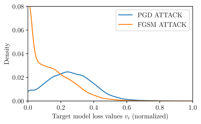
(a) Distribution of $f_{t}$’s loss values.

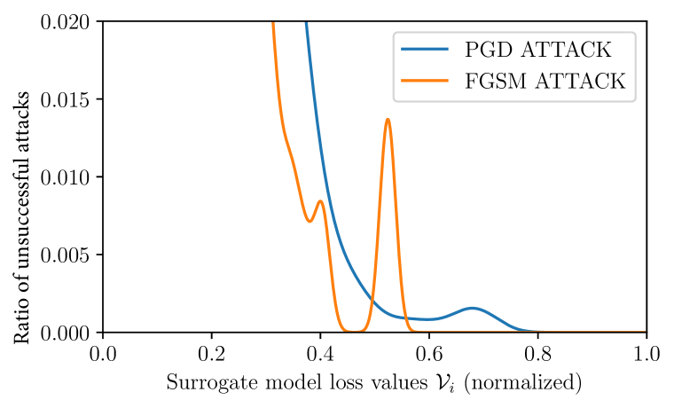
(b) Ratio of unsuccessful attacks.

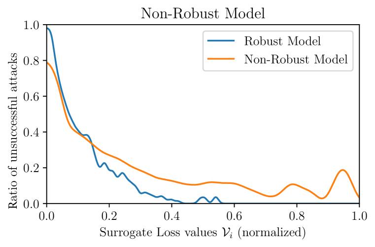
(c) Ratio of unsuccessful attacks.

Figure 5: For every example in MNIST we compute an attack using $f_{s}$ and submit it to $f_{t}$. Left: The distribution of the normalized loss values of $f_{t}$ for all attacks where a higher loss is a stronger attack. Middle: The percentage of unsuccessful attacks as a function of $f_{s}$ normalized loss values. Right: smoothed ratio of unsuccessful attacks to total attacks as a function of the $f_{s}$ normalized loss values.

6 Conclusion

In this paper, we formulate the online adversarial attack problem, a novel threat model to study adversarial attacks on streaming data. We propose Virtual+, a simple yet practical online algorithm that enables attackers to select easy to fool data points while being theoretically the best single threshold algorithm for $k<5$. We further introduce the stochastic $k$-secretary problem and prove fundamental results on the competitive ratio of any online algorithm operating in this new setting. Our work sheds light on the tight coupling between optimally selecting data points using an online algorithm and the final attack success rate, enabling weak adversaries to perform on par with stronger ones at no additional cost. Investigating, the optimal threshold values for larger values of $k$ along with competitive analysis for the general setting is a natural direction for future work.

Ethics Statement

We introduce the online threat model which aims to capture a new domain for adversarial attack research against streaming data. Such a threat model exposes several new security and privacy risks. For example, using online algorithms, adversaries may now tailor their attack strategy to attacking a small subset of streamed data but still cause significant damage to downstream models e.g. the control system of an autonomous car. On the other hand our research also highlights the need and importance of stateful defence strategies that are capable of mitigating such online attacks. On the theoretical side the development and analysis of Virtual+ has many potential applications outside of adversarial attacks broadly categorized as resource allocation problems. As a concrete example one can consider advertising auctions which provide the main source of monetization for a variety of internet services including search engines, blogs, and social networking sites. Such a scenario is amenable to being modelled as a secretary problem as an advertiser may be able to estimate accurately the bid required to win a particular auction, but may not be privy to the trade off for future auctions.

Reproducibility statement

Throughout the paper we tried to provide as many details as possible in order for the results of the paper to be reproducible. In particular, we provide a detailed description of Virtual+in Alg. 1 and we explain how to combine any attacker (e.g. PGD) with an online algorithm to form an online adversarial attack in Alg. 2. We provide a general description of the experimental setup in §5, further details with the specific architecture of the models and hyper-parameters used are provided in §E.3. We also provided confidence intervals with our experiments every time it was possible to do so. Finally the code used to produce the experimental results is provided with the supplementary materials and will be made public after the review process.

Contributions

Andjela Mladenovic and Gauthier Gidel formulated the online adversarial attacks setting by drawing parallels to the $k$-secretary problem, with Andjela Mladenovic leading the theoretical investigation and theoretical results including the competitive analysis for Virtual+ for the general-$k$ setting. Avishek Joey Bose conceived the idea of online attacks, drove the writing of the paper and helped Andjela Mladenovic with experimental results on synthetic data. Hugo Berard was the chief architect behind all experimental results on MNIST and CIFAR-10. William L. Hamilton, Simon Lacoste-Julien and Pascal Vincent provided feedback and guidance over this research while Gauthier Gidel supervised the core technical execution of the theory.

Appendix A Proof of Competitive Ratio for Virtual+Algorithm

As an illustrative example that aids in understanding the full general-$k$ proof for for the competitive ratio Virtual+ we now prove Theorem 1 for $k=2$ from the main paper.

Theorem 3.

For $k=2$, the competitive ratio achieved by Virtual+ algorithm is equal to,

$$C_{n}=\frac{t(t-1)}{n}\sum_{j=t}^{n-1}\frac{1}{j(j-1)}\left(1+2\sum_{p=t+1}^{j}\frac{1}{p-1}\right)$$ (6)

Particularly for $t=\alpha\cdot n\,,\,\alpha\in(0,1)$ we get

$$C_{n}>\alpha(3(1-\alpha)+2\alpha\ln(\alpha))+\mathcal{O}(1/n)$$ (7)

Thus, asymptotically we have

$$C>\max_{\alpha\in[0,1]}\alpha(3(1-\alpha)+2\alpha\ln(\alpha))>.4273>1/e\,.$$ (8)

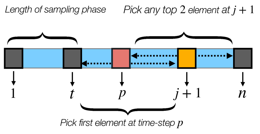
Figure 6: Probability of having only one element in $S_{\mathcal{A}}$ after $j$ time-steps with the Virtual+ algorithm.

Proof.

First note that by Albers & Ladewig (2020, Lemma 3.3) we can show that the competitive ratio for the $k$-secretary problem for a monotone algorithm is equal to

$$C=\frac{1}{k}\sum_{a=1}^{k}\mathbb{P}(i_{a}\in S_{\mathcal{A}}),$$ (9)

where $i_{a}$ is the index of the $a^{th}$ secretary picked by the offline solution —i.e. $i_{a}$ is a top-$k$ secretary of $\mathcal{D}$. By Lemma 2 Virtual+ is a monotone algorithm and we may use  Eq. 9. Now, let us focus on the case $k=2$. When calculating the probability of either of the top two items in $\mathcal{D}$ being picked by the Virtual+ we must first compute the probability of one of the top-2 items being picked during the selection phase (time step $t+1\dots n$). Now notice that Virtual+ picks an item at time step $j+1$ if and only if this is a top-2 item with respect to all of $\mathcal{D}$ and $|S_{\mathcal{A}}|\leq 2$ at time-step $j+1$. Let top-$2_{j}$ denote the two largest elements observed by $\mathcal{A}$ up to and inclusive of time step $j$. Thus, for $a\in\{1,2\}$, we have

$$\mathbb{P}(i_{a}\in S_{\mathcal{A}}) =\sum_{j=t}^{n-1}\mathbb{P}(i_{a}\in S_{\mathcal{A}}\text{ at time-step }j+1)$$ (10)

$$=\frac{1}{n}\sum_{j=t}^{n-1}\mathbb{P}(|S_{\mathcal{A}}|<2\text{ at time-step }j+1)$$

Now, we compute $\mathbb{P}(|S_{\mathcal{A}}|\leq 2\text{ at time-step }j+1)$ by decomposing this probability into the following two events: A.) $|S_{\mathcal{A}}|=0$ where the selection set is empty and B.) the event $|S_{\mathcal{A}}|=1$ where exactly one item has been picked. We now analyze each event in turn.

Event A. In order for the event $|S_{\mathcal{A}}|=0$ to occur it implies that the algorithm does not select any items in the first $j$ rounds. This means both two top-$2_{j}$ elements must have appeared in the sampling phase. Thus the probability for this event is exactly $\frac{t(t-1)}{j(j-1)}$.

Event B. The second event is when $|S_{\mathcal{A}}|=1$ —i.e. the algorithm picks exactly one element in the first $j$ rounds. The computation of this event is illustrated in Figure 6. Let’s say that an element is picked at time step $p$. Now to compute the probability of Event B occurring we first make the following two observations:

1. In order for exactly one element to be picked at the time step $p\leq j$, this element must be one of the top-$2_{j}$ elements. Furthermore, this implies the other of the top-$2_{j}$ element —i.e. the one not picked at $p$ must have appeared in the sampling phase. Note that if both top-$2_{j}$ elements appear after the sampling phase, the condition would be satisfied twice and two elements would be selected instead of exactly one, and if they both appeared during the sampling phase we return to Event A. As a result, the probability for this condition is given by $\frac{t}{j(j-1)}$.

2. By observation 1. we know that the online algorithm $\mathcal{A}$ picks one of the top-$2_{j}$ at time step $p$ and the fact that the event under consideration is $|S_{\mathcal{A}}|=1$ the reference list $R$ from time step $p$ to $j+1$ must contain both top-$2_{j}$ elements. However, for $\mathcal{A}$ to pick only at $p$ we also need to ensure that no elements are picked prior t to $p$. Therefore, before time step $p$ the reference list must contain top-$2_{p}$ . Again by observation 1, we know that $R$ already contains one of the top-$2_{j}$ elements therefore we know it contains one of the top-$2_{p}$ elements. Thus the probability of ensuring that the second top-$2_{p}$ elements is also within $R$ by time step $p$ is $\frac{(t-1)}{(p-2)}$. Finally, since there are two top elements and they may appear in any order we must count the probability of Event B occurring twice.

Overall we get:

$$\frac{t(t-1)}{j(j-1)}+2\sum_{p=t+1}^{j}\frac{1}{j}\frac{t}{j-1}\frac{t-1}{p-2}$$ (11)

Total probability:

$$\frac{1}{n}\sum_{j=t}^{n-1}\left(\frac{t(t-1)}{j(j-1)}+2\sum_{p=t+1}^{j}\frac{1}{j}\frac{t}{j-1}\frac{t-1}{p-2}\right) =\frac{1}{n}\sum_{j=t}^{n-1}\left(1+2\sum_{p=t}^{j-1}\frac{1}{p-1}\right)$$

$$=\frac{t(t-1)}{n}\sum_{j=t}^{n-1}\left(\frac{1}{j(j-1)}+\frac{2}{j(j-1)}\sum_{p=t}^{j-1}\frac{1}{p-1}\right)$$

$$>\frac{t(t-1)}{n}\sum_{j=t}^{n-1}\left(\frac{1}{j^{2}}+2\frac{1}{j^{2}}\sum_{p=t+1}^{j}\frac{1}{p-1}\right)$$

$$>\frac{t(t-1)}{n}\sum_{j=t}^{n-1}\left(\frac{1}{j^{2}}+\frac{2}{j^{2}}\int_{p=t+1}^{j+1}\frac{1}{p-1}\,dp\right)$$

$$>\frac{t(t-1)}{n}\sum_{j=t}^{n-1}\left(\frac{1}{j^{2}}+\frac{2}{j^{2}}\ln\left(\frac{j}{t}\right)\right)$$

Now we will use the following lemma

Lemma 1.

For any differentiable function $f$ and any $a<b$, we have,

$$\sum_{j=a}^{b}f(j)\geq\int_{a}^{b+1}f(t)dt-|b+1-a|\sup_{t\in[a,b+1]}|f^{\prime}(t)|$$ (12)

Proof.

$$|f(n)-\int_{n}^{n+1}f(t)dt|\leq\int_{n}^{n+1}|f(n)-f(t)|dt\leq\sup_{t\in[n,n+1]}|f^{\prime}(t)|$$ (13)

Thus,

$$f(n)\geq\int_{n}^{n+1}f(t)dt-\sup_{t\in[n,n+1]}|f^{\prime}(t)|$$ (14)

and by summing for $n=a\ldots b$ we get the desired lemma. ∎

Applying this lemma to $f(x)=\frac{1+2\ln(x/t)}{x^{2}}\,,a=t$ and $b=n-1$, we get

$$\frac{1}{n}\sum_{j=t}^{n-1}\frac{t(t-1)}{j(j-1)}+2\sum_{p=t+1}^{j}\frac{1}{j}\frac{t}{j-1}\frac{t-1}{p-2} >\frac{t(t-1)}{n}\sum_{j=t}^{n-1}\left(\frac{1}{j^{2}}+\frac{2}{j^{2}}\ln\left(\frac{j}{t}\right)\right)$$ (15)

$$\geq\frac{t(t-1)}{n}\left(\int_{t}^{n}\frac{1+2\ln(x/t)}{x^{2}}dx-2(n-t)\sup_{x\in[t,n]}\left|\frac{4\ln(x/t)}{x^{3}}\right|\right)$$

$$\geq\frac{t(t-1)}{n}\left(\int_{t}^{n}\frac{1+2\ln(x/t)}{x^{2}}dx-2(n-t)\left|\frac{16}{3t^{3}e^{4}}\right|\right)$$

$$=\frac{t(t-1)}{n}\left(\frac{3}{t}-\frac{2\ln(n/t)+3}{n}-2(n-t)\left|\frac{16}{3t^{3}e^{4}}\right|\right)$$ (16)

Now for $t=\alpha n$ where $\alpha\in(0,1)$ and as $n\xrightarrow[]{}\infty$, that lower-bound becomes

$$C\geq\alpha(3-\alpha(3-2\ln(\alpha)))+\mathcal{O}(1/n)\,,\quad\forall\alpha\in(0,1)$$ (17)

The constant term of the RHS is a concave function of $\alpha$ that is maximized for $\alpha^{*}\approx 0.38240$. Thus, our algorithms achieves competitive ratio larger than $0.42737$. ∎

Appendix B Competitive Ratio General $k$

We now prove our main result for the competitive ratio of Virtual+ for $k\geq 2$. The theorem statement is reproduced here for convenience.

Theorem 1.

The competitive ratio of Virtual+ for $k\geq 2$ with threshold $t_{k}=\alpha n$ can asymptotically be lower bounded by the following concave optimization problem,

$$C_{k}>\max_{\alpha\in[0,1]}f(\alpha):={\alpha}^{k}\left(\sum_{m=0}^{k-1}a_{m}\ln^{m}(\alpha)\right)-\alpha a_{0}\hskip 4.26773ptwhere\hskip 4.26773pta_{m}=\left(\frac{\frac{k^{k}}{(k-1)^{k-m}}-k^{m}}{m!}\right)(-1)^{m+1}\,.$$

Particularly, we get $C_{2}\geq 0.427,C_{3}\geq.457,C_{4}\geq.4769$ outperforming Albers & Ladewig (2020).

Figure 7: Virtual+ $k\geq 2$ proof.

Proof.

First note that by Albers & Ladewig (2020, Lemma 3.3) we can show that the competitive ratio for the $k$-secretary problem for a monotone algorithm is equal to

$$C=\frac{1}{k}\sum_{a=1}^{k}\mathbb{P}(i_{a}\in S_{\mathcal{A}}),$$ (18)

where $i_{a}$ is the index of the $a^{th}$ secretary picked by the optimal offline solution —i.e. $i_{a}$ is a top-$k$ secretary of $\mathcal{D}$. By Lemma 2 Virtual+ is a monotone algorithm and we may use  Eq. 18.

$$\mathbb{P}(i_{a}\in S_{\mathcal{A}}) =\sum_{j=t}^{n-1}\mathbb{P}(i_{a}\in S_{\mathcal{A}}\text{ at time-step }j+1)$$ (19)

$$=\frac{1}{n}\sum_{j=t}^{n-1}\mathbb{P}(|S_{\mathcal{A}}|<k\text{ at time-step }j+1)$$

Now, we compute $\mathbb{P}(|S_{\mathcal{A}}|<k\text{ at time-step }j+1)$ by decomposing this probability into smaller events $\mathbb{P}(|S_{\mathcal{A}}|=\nu\text{ at time-step }j+1)$ where $\nu\in[0,\dots,k-1]$.

We may compute the probability of $\mathbb{P}(|S_{\mathcal{A}}|=\nu\text{ at time-step }j+1)$ in the following manner. First, let us consider the scenario where $\nu$ elements are selected by Virtual+ at time steps $p_{1}$, $p_{2},\dots,p_{\nu}$. Now, in order for an element to be selected at position $p_{\nu}$ that element must be one of the top $k$ elements up to time-step $j+1$. Therefore we have a factor $k/j$ in our equation. Now, in order to guarantee that no elements are picked after the position $p_{\nu}$ we additionally need to ensure that the remaining top-$k$ up to $j+1$ elements appear before $p_{\nu}$ which results in a factor of ${p_{\nu}-1\choose k-1}/{j-1\choose k-1}$. Similarly, we may recursively calculate the corresponding factor for each position $p_{\nu-1}\dots p_{1}$. However, we also need to guarantee that no elements are picked within the time interval $[t+1\dots p_{1}-1]$ —i.e. before $p_{1}$. The probability for this occurring is then ${t\choose k}/{p_{1}-1\choose k}$ as this corresponds an ordering where the top-$k$ elements up to $p_{1}-1$ all appear in the sampling phase. Thus, the probability $p_{t,j}^{k,\nu}:=\mathbb{P}(|S_{\mathcal{A}}|=\nu\text{ at time-step }j+1)$ is :

$$p_{t,j}^{k,\nu} =\sum_{t+1\leq p_{1}<p_{2}<\dots<p_{k-1}\leq j}\frac{k}{j}\frac{{p_{\nu}-1\choose k-1}}{{j-1\choose k-1}}\frac{k}{p_{\nu}-1}\frac{{p_{{\nu}-1}-1\choose k-1}}{{p_{\nu}-2\choose k-1}}\frac{k}{p_{\nu-1}-1}\dots\frac{k}{p_{2}-1}\frac{{p_{1}-1\choose k-1}}{{p_{2}-2\choose k-1}}\frac{{t\choose k}}{{p_{1}-1\choose k}}$$ (20)

$$=\frac{t(t-1)\dots(t-k+1)}{j(j-1)\dots(j-k+1)}\sum_{t+1\leq p_{1}<p_{2}<\dots<p_{\nu}\leq j}\frac{k^{\nu}}{(p_{\nu}-k)(p_{\nu-1}-k)\dots(p_{1}-k)}$$ (21)

Therefore, the probability of not exceeding $k$-selections, $p_{t,j}^{k}=\sum_{\nu=0}^{k-1}p_{t,j}^{k,\nu}$, to get before time step $j+1$ is:

$$p_{t,j}^{k} =\frac{t(t-1)...(t-k+1)}{j(j-1)\dots(j-k+1)}\bigg{(}1+k\sum_{p_{1}=t+1\dots j}\Lambda_{p_{1}}+\dots+{k^{k-1}}\sum_{\begin{subarray}{c}p_{1}=t+1\dots p_{2}-1\\ \vdots\\ p_{k-1}=t+1\dots j\end{subarray}}\Lambda_{p_{1}}\dots\Lambda_{p_{k-1}}\bigg{)},$$

where we define $\Lambda_{p_{i}}:=\frac{1}{p_{i}-k}$. The total competitive ratio is then:

$$C_{k} =\frac{1}{n}\sum_{j=t}^{n-1}\frac{t(t-1)\dots(t-k+1)}{j(j-1)\dots(j-k+1)}\bigg{(}1+k\sum_{p_{1}=t+1\dots j}\Lambda_{p_{1}}+\dots+{k^{k-1}}\sum_{\begin{subarray}{c}p_{1}=t+1\dots p_{2}-1\\ \vdots\\ p_{k-1}=t+1\dots j\end{subarray}}\Lambda_{p_{1}}\dots\Lambda_{p_{k-1}}\bigg{)},$$ (22)

Now using Lemma  3 we can bound it:

$$C_{k} \geq\frac{1}{n}\int_{j=t}^{n}\frac{t(t-1)\dots(t-k+1)}{j(j-1)\dots(j-k+1)}\bigg{(}1+\frac{k}{1!}\ln\Big{(}\frac{j-k}{t}\Big{)}+\dots+\frac{k^{k-1}}{(k-1)!}\ln^{k-1}\Big{(}\frac{j-k}{t}\Big{)}\bigg{)}$$ (23)

$$\geq\frac{1}{n}\int_{j=t}^{n}\frac{t(t-1)\dots(t-k+1)}{j^{k}}\bigg{(}1+\frac{k}{1!}\ln\Big{(}\frac{j-k}{t}\Big{)}+\dots+\frac{k^{k-1}}{(k-1)!}\ln^{k-1}\Big{(}\frac{j-k}{t}\Big{)}\bigg{)}$$ (24)

Now notice that:

$$\int\frac{1}{a!}\frac{\ln^{a}(x)}{x^{k}}dx=-\frac{1}{x^{k-1}}\sum_{m=0}^{a}\frac{1}{m!}(k-1)^{m-1-a}\ln^{m}(x)$$ (25)

Using the identity in  Eq. 25 we compute the competitive ratio as:

$$\geq\frac{t(t-1)\dots(t-k+1)}{n}\bigg{(}\sum_{a=0}^{k-1}-\frac{1}{j^{k-1}}{k^{a}}\sum_{m=0}^{a}\frac{1}{m!}(k-1)^{m-1-a}\ln^{m}\Big{(}\frac{j-k}{t}\Big{)}\bigg{)}\Big{|}_{j=t}^{n}$$ (26)

$$=\frac{t(t-1)\dots(t-k+1)}{n}\bigg{(}-\frac{1}{j^{k-1}}\sum_{m=0}^{k-1}\frac{1}{m!}\Big{(}\sum_{a=m}^{k-1}{k^{a}}(k-1)^{m-a-1}\Big{)}\ln^{m}{\Big{(}\frac{j-k}{t}\Big{)}}\bigg{)}\Big{|}_{j=t}^{n}$$ (27)

For threshold $t=\alpha n$ where $\alpha\in(0,1)$ and as $n\xrightarrow{}\infty$ our competitive rate becomes:

$$\alpha\bigg{(}\sum_{a=0}^{k-1}{k^{a}}{(k-1)}^{-1-a}\Big{)}-\alpha^{k}\Big{(}\sum_{m=0}^{k-1}\frac{1}{m!}\Big{(}\sum_{a=m}^{k-1}{k^{a}}(k-1)^{m-a-1}\Big{)}\ln^{m}\Big{(}\frac{1}{\alpha}\Big{)}\bigg{)}$$ (28)

$$=\alpha\left({\left(\frac{k}{k-1}\right)}^{k}-1\right)-\alpha^{k}\left(\sum_{m-0}^{k-1}\left(\frac{\frac{k^{k}}{(k-1)^{k-m}}-k^{m}}{m!}\right)(-1)^{m+1}\ln^{m}(\alpha)\right)$$ (29)

Finally let us show that

$$f(\alpha):={\alpha}^{k}\left(\sum_{m=0}^{k-1}a_{m}\ln^{m}(\alpha)\right)-\alpha a_{0}\quad where\quad a_{m}=\left(\frac{\frac{k^{k}}{(k-1)^{k-m}}-k^{m}}{m!}\right)(-1)^{m+1}$$ (30)

is concave. To do so we just compute it second derivative and show that $f^{\prime\prime}(\alpha)\leq 0$. We have,

$$f^{\prime\prime}(\alpha) =\alpha^{k-2}\sum_{m=0}^{k-3}\left[k(k-1)a_{m}+(2k-1)(m+1)a_{m+1}+(m+1)(m+2)a_{m+2}\right]\ln^{m-2}(\alpha)$$

$$\quad+[k(k-1)a_{k-2}+(2k-1)(k-1)a_{k-1}]\ln^{k-2}(\alpha)+k(k-1)a_{k-1}\ln^{k-1}(\alpha)\,.$$

By using the definition of $a_{m}$, we can verify that

$$k(k-1)a_{m}+(2k-1)(m+1)a_{m+1}+(m+1)(m+2)a_{m+2}=0$$

$$\text{and}\quad k(k-1)a_{k-2}+(2k-1)(k-1)a_{k-1}=0\,.$$

Thus we finally get,

$$f^{\prime\prime}(\alpha)=k(k-1)a_{k-1}\ln^{k-1}(\alpha)=-\frac{k^{2}\big{(}\alpha k\log(\frac{1}{\alpha})\big{)}^{k-1}}{\alpha k!}\leq 0$$ (31)

where we use the fact that since $\alpha\in[0,1]$, we have $\alpha\log(1/\alpha)\geq 0$. ∎

Definition B.1.

An algorithm is called monotone if the probabilities of selecting items $i$ and $j$ satisfy $p_{i}\geq p_{j}$ whenever the item values $v_{i}>v_{j}$ holds for any two items.

Lemma 2.

Virtual+ is a monotone algorithm.

Proof.

In order to prove that Virtual+ is monotone as defined in Definition B.1 we must prove that $p_{i}\geq p_{j}$ (where $p_{i}$ is the probability of picking the item $i$) for any two items where $v_{i}>v_{j}$. Without loss of generality let us consider a decreasing ordering of $n$-elements based on their values —i.e. $v_{1}>v_{2}>\dots>v_{n}$.

We prove that $p_{i}\geq p_{i+1}$ for all $i\in[1,\dots,n-1]$ by showing that for each input sequence where $v_{i+1}$ is accepted, there exists a unique input sequence where $v_{i}$ is accepted. Let us consider a permutation $\pi$ where $v_{i+1}$ appeared and was accepted at time step $a$ while $v_{i}$ appeared at time step $b$. By swapping $v_{i}$ and $v_{i+1}$ we obtain a new permutation $\pi^{\prime}$ where $v_{i}$ now appears at $a$ and $v_{i+1}$ at $b$. We now study the two following cases.

Case 1: $a<b$.

If $a<b$ notice that the reference set, $R$, and the selected set $S_{\mathcal{A}}$, are exactly the same at time step $a$ for both permutations $\pi$ and $\pi^{\prime}$. Therefore, if $v_{i+1}$ was accepted at time step $a$ in permutation $\pi$ then $v_{i}$ will also be accepted at time step $a$ in permutation $\pi^{\prime}$ since $v_{i}>v_{i+1}$.

Case 2: $a>b$.

If $a>b$ notice that $R$—by definition of Virtual+—at time step $a$ contains top-$k$ elements observed in the first $a-1$ time steps. Now the $k$-th element in $R$ at time-step $a$ must satisfy,

$$R^{a}_{\pi}[k]\geq R^{a}_{\pi^{\prime}}[k],$$

where $R^{a}_{[\cdot]}[k]$ corresponds to the $k$-element in the reference set for a specific permutation at time step $a$. Hence, we know that $v_{i}>v_{i+1}\geq R^{a}_{\pi}[k]\geq R^{a}_{\pi^{\prime}}[k]$ as $v_{i+1}$ was assumed to be picked.

Furthermore, the $S_{\mathcal{A}}$ and $R$ is the same for permutations $\pi$ and $\pi^{\prime}$ at time-step $b$. Now by our primary assumption that $v_{i+1}$ is picked at time-step $a>b$ in $\pi$ this means that $v_{i}$ must be $v_{i}\geq R^{b}_{\pi}[k]$ since $v_{i}>v_{i+1}$. However, observe that $v_{i}$ and $R^{b}_{\pi}[k]$ cannot be consecutive in value as $v_{i+1}$ appears at time-step $a>b$ in permutation $\pi$. This implies that $v_{i+1}$ must also be selected at time step $b$ in permutation $\pi^{\prime}$ since $v_{i}$ and $v_{i+1}$ are consecutive in value. By a similar argument based on consecutive order of values between time steps $a$ and $b$ precisely the same elements will be selected in both $\pi$ and $\pi^{\prime}$. The argument that $v_{i}>v_{i+1}\geq R^{a}_{\pi}[k]\geq R^{a}_{\pi^{\prime}}[k]$ implies that if $v_{i+1}$ is selected in permutation $\pi$, $v_{i}$ will also be selected in permutation $\pi^{\prime}$. The claim then follows by applying the inequality $p_{i}\geq p_{i+1}$ in an iterative fashion. ∎

Lemma 3.

Let $f_{i}\,,\,i=1\ldots k$ be decreasing positive functions then we have

$$\sum_{p_{1}=a_{1}}^{b_{1}}\ldots\sum_{p_{k}=a_{k}}^{p_{k-1}}f_{1}(p_{1})\ldots f_{k}(p_{k})\geq\int_{x_{1}=a_{1}}^{b_{1}+1}\ldots\int_{x_{k}=a_{k}}^{x_{k-1}+1}f_{1}(x_{1})\ldots f_{k}(x_{k})dx_{1}\dots dx_{k}$$ (32)

Proof.

The main proof step involves in first noticing that since the functions $f_{i}\,,\,i=1\ldots k$ are decreasing and are positive we have,

$$f_{1}(p_{1})\ldots f_{k}(p_{k})\geq f_{1}(p_{1})\ldots f_{k-1}(p_{k-1})\int_{x_{k}=p_{k}}^{p_{k}+1}f_{k}(x_{k})dx_{k}$$ (33)

Thus, by summing this inequality for $p_{k}=a_{k}\ldots p_{k-1}$, we get

$$\sum_{p_{k}=a_{k}}^{p_{k-1}}f_{1}(p_{1})\ldots f_{k}(p_{k})\geq f_{1}(p_{1})\ldots f_{k-1}(p_{k-1})\int_{x_{k}=a_{k}}^{p_{k-1}+1}f_{k}(x_{k})dx_{k}$$ (34)

Now, because the functions $f_{i}\,,\,i=1\ldots k$ are decreasing and positive we have,

$$\mathcal{S} =\sum_{p_{k}=a_{k}}^{p_{k-1}}f_{1}(p_{1})\ldots f_{k}(p_{k})$$ (35)

$$\geq f_{1}(p_{1})\ldots f_{k-2}(p_{k-2})\int_{x_{k-1}=p_{k-1}}^{p_{k-1}+1}f_{k-1}(x_{k-1})\int_{x_{k}=a_{k}}^{p_{k-1}+1}f_{k}(x_{k})dx_{k-1}dx_{k}$$ (36)

$$\geq f_{1}(p_{1})\ldots f_{k-2}(p_{k-2})\int_{x_{k-1}=p_{k-1}}^{p_{k-1}+1}f_{k-1}(x_{k-1})\int_{x_{k}=a_{k}}^{x_{k-1}}f_{k}(x_{k})dx_{k-1}dx_{k}$$ (37)

where for the last inequality we used the fact that $x_{k-1}\in[p_{k-1},p_{k-1}+1]$. Finally, by summing for $p_{k-1}=a_{k-1}\ldots p_{k-2}$, we get,

$$\sum_{p_{k-1}=a_{k-1}}^{p_{k-2}}\mathcal{S} =\sum_{p_{k-1}=a_{k-1}}^{p_{k-2}}\sum_{p_{k}=a_{k}}^{p_{k-1}}f_{1}(p_{1})\ldots f_{k}(p_{k})$$ (38)

$$\geq f_{1}(p_{1})\ldots f_{k-2}(p_{k-2})\int_{x_{k-1}=p_{k-1}}^{p_{k-1}+1}f_{k-1}(x_{k-1})\int_{x_{k}=a_{k}}^{x_{k-1}}f_{k}(x_{k})dx_{k-1}dx_{k}$$ (39)

Using a recursive argument we finally get,

$$\sum_{p_{1}=a_{1}}^{b_{1}}\ldots\sum_{p_{k}=a_{k}}^{p_{k-1}}f_{1}(p_{1})\ldots f_{k}(p_{k})\geq\int_{x_{1}=a_{1}}^{b_{1}+1}\ldots\int_{x_{k}=a_{k}}^{x_{k-1}+1}f_{1}(x_{1})\ldots f_{k}(x_{k})dx_{1}\dots dx_{k}$$ (40)

∎

B.1 Analytic computation of $C_{k}$ for Virtual+

Table 3: Values of the Competitive ratio $C_{k}$ and the associated optimal $\alpha_{k}$ needed to compute the threshold for Virtual+. Note that for $5\leq k\leq 100$ the competitive ratio of Single-Ref provided by Albers & Ladewig (2020) outperforms Virtual+’s competitive ratio. However, our analysis provides a tractable way to scale the analytic computation of the competitive ratio with $k$ as the function to optimize (and its gradients) in Theorem 1 is $\mathcal{O}(k)$.

$k$	2	3	4	5	100	200	300	400	500	600
$C_{k}$	.4273	.4575	.4769	.4906	.5959	.6062	.6108	.6136	.6156	.6170
$\alpha_{k}$	.3824	.3867	.3884	.3890	.3781	.3755	.3743	.3735	.3729	.3726

Appendix C Proof of Theorem 2 and empirical verification

We now prove Theorem 2 in detail, reproduced here for convenience.

Theorem 2.

Let us assume that Virtual+ observes independent random variables $\mathcal{V}_{i}$ following Assumption 1. Its stochastic competitive ratio $C_{s}$ can be bounded as follows,

$$C\geq C_{s}\geq\gamma C$$ (41)

Proof.

In the Stochastic case we use the same beginning proof as in the non-stochastic case until Eq. 19. Let us consider $i_{a}$ such that $\mathcal{V}_{i_{a}}\in\operatorname*{top_{k}}\{\mathcal{V}_{i}\}$,

$$\mathbb{P}(i_{a}\in S_{\mathcal{A}}) =\sum_{j=t}^{n-1}\mathbb{P}(i_{a}\in S_{\mathcal{A}}\text{ at time-step }j+1)$$ (42)

Now, in the stochastic case $\mathbb{P}(i_{a}\in S_{\mathcal{A}}\text{ at time-step }j+1)$ not only depends on the set $\mathcal{S}_{\mathcal{A}}$ not being full but also that $i_{a}$ corresponds to a top-$k$ elements in $\{v_{i}\}$. Because of the expectation over permutations, the event of the knapsack being fulled at time step $j+1$ is independent from what happens at timestep $j+1$. Thus we can write that

$$\mathbb{P}(i_{a}\in S_{\mathcal{A}}\text{ at time-step }j+1) =\mathbb{P}(|S_{\mathcal{A}}|<k\text{ at time-step }j+1){\mathbb{P}}[\mathcal{V}_{i}\in\operatorname*{top_{k}}\{\mathcal{V}_{i}\}\,|\,v_{i}\in\operatorname*{top_{k}}\{v_{i}\}]$$

$$\geq\mathbb{P}(|S_{\mathcal{A}}|<k\text{ at time-step }j+1)\gamma\,.$$

Finally, we just need to notice that ${\mathbb{P}}[\mathcal{V}_{i}\in\operatorname*{top_{k}}\{\mathcal{V}_{i}\}\,|\,v_{i}\in\operatorname*{top_{k}}\{v_{i}\}]$ does not depend on the value observed and thus leave to the same computation as in the non-stochastic case.

Similarly, we have

$$\mathbb{P}(i_{a}\in S_{\mathcal{A}}\text{ at time-step }j+1) =\mathbb{P}(|S_{\mathcal{A}}|<k\text{ at time-step }j+1){\mathbb{P}}[\mathcal{V}_{i}\in\operatorname*{top_{k}}\{\mathcal{V}_{i}\}\,|\,v_{i}\in\operatorname*{top_{k}}\{v_{i}\}]$$

$$\leq\mathbb{P}(|S_{\mathcal{A}}|<k\text{ at time-step }j+1)\,.$$

In conclusion it leads to

$$C\geq C_{s}\geq\gamma C$$ (43)

∎

C.1 Empirical Quantification of Assumption 1

Assumption 1 requires that a percentage of top-$k$ true values $v_{i}$ remain top-$k$ under noise. We now empirically quantify the strength of this assumption in both of our datasets MNIST and CIFAR-10. Note that unlike in theorem we cannot enforce any structure on the random variables that act as surrogate losses as provided by $f_{s}$. Despite this, we find that in all cases the overlap between the top-$k$ sets is non-zero which enables the effective use of online algorithms for picking candidate attack points as shown in table LABEL:app:table_with_overlap.

Table 4: Number of top-$k$ elements in $\{v_{i}\}$ that are also top-$k$ elements in $\{\mathcal{V}_{i}\}$ for the different setting considered in the paper. $|\operatorname*{top_{k}}\{\mathcal{V}_{i}\}\cap\operatorname*{top_{k}}\{v_{i}\}|$ Note that $n=10000$.

	MNIST			CIFAR-10
	$k=10$	$k=100$	$k=1000$	$k=10$	$k=100$	$k=1000$
FGSM	0.9 $\pm$ 0.1	16.1 $\pm$ 0.7	324.0 $\pm$ 7.0	0.60 $\pm$ 0.03	12.5 $\pm$ 0.2	333.2 $\pm$ 2.8
PGD	0.58 $\pm$ 0.03	7.1 $\pm$ 0.3	229.9 $\pm$ 3.3	0.59 $\pm$	10.0 $\pm$ 0.3	227.1 $\pm$ 3.6

Appendix D Classical Online Algorithms for Secretary Problems

All single threshold online algorithm described in this paper include: Virtual, Optimistic and Single-Ref. Each online algorithm consists of two phases —sampling phase followed by selection phase— and an optimal stopping point $t$ which is used by the algorithm to transition between the phases. We now briefly summarize these two phases for the aforementioned online algorithms.

Sampling Phase - Virtual, Optimistic and Single-Ref. In the sampling phase, the algorithms passively observe all data points up to a pre-specified time index $t$, but also maintains a sorted reference list $R$ consisting of the $k$ elements with the largest values $\mathcal{V}(i)$ seen. Thus the $R$ contains a list of elements sorted by decreasing value. That is $R[k]$ is the index of the $k$-th largest element in $R$ and $\mathcal{V}(R[k])$ is its corresponding value. The elements in $R$ are kept for comparison but are crucially not selected in the sampling phase.

D.1 Virtual Algorithm

Selection Phase - Virtual algorithm. Subsequently, in the selection phase, $i>t$, when an item with value $\mathcal{V}(i)$ is observed an irrevocable decision is made of whether the algorithm should select $i$ into $S$. To do so, the Virtual algorithm simply checks if the value of the $k$-th smallest element in $R$, $\mathcal{V}(R[k])$, is smaller than $\mathcal{V}(i)$ in addition to possibly updating the set $R$. The full Virtual algorithm is presented in Algorithm 1.

Inputs: $t\in[k\dots n-k]$, $R=\emptyset$, $S_{\mathcal{A}}=\emptyset$
Sampling phase: Observe the first $t$ data points and construct a list $R$ with the indices of the top $k$ data points seen. sort ensures: $\mathcal{V}(R[1])\geq\mathcal{V}(R[2])\dots\geq\mathcal{V}(R[k]).$

Selection phase (at time $i>t$):

1:  if $\mathcal{V}(i)\geq\mathcal{V}(R[k])$ and $R[k]>t$ then

2:     $R$ = $\texttt{sort}\{R\cup\{i\}\setminus\{R[k]\}\}$ {// Update $R$ with element $i$ and also take out $R[k]$}

3:  else if  $\mathcal{V}(i)\geq\mathcal{V}(R[k])$ and $R[k]\leq t$ then

4:     $R$ = $\texttt{sort}\{R\cup\{i\}\setminus\{R[k]\}\}$ {// Update $R$ with element $i$ and also take out $R[k]$}

5:     $S_{\mathcal{A}}=\{S_{\mathcal{A}}\cup\{i\}\}$ {// Select element $i$}

6:  $i\leftarrow i+1$

Algorithm 3 Virtual Algorithm

D.2 Optimistic Algorithm

Selection Phase - Optimistic algorithm. In the optimistic algorithm, i is selected if and only if $\mathcal{V}(i)\geq\mathcal{V}(R[last])$. Whenever $i$ is selected, $R[last]$ is removed from the list $R$, but no new elements are ever added to $R$. Thus, intuitively, elements are selected when they beat one of the remaining reference points from $R$. We call this algorithm “optimistic” because it removes the reference point $R[last]$ even if $\mathcal{V}(i)$ exceeds, say, $\mathcal{V}(R[1])$. Thus, it implicitly assumes that it will see additional very valuable elements in the future, which will be added when their values exceed those of the remaining, more valuable, $R[a]\,,\,a\in[k]$.

Inputs: $t\in[k\dots n-k]$, $R=\emptyset$, $S_{\mathcal{A}}=\emptyset$.

Sampling phase (up to time $t$): Observe the first $t$ data points and construct a list $R$ with the indices of the top $k$ data points seen. sort ensures: $\mathcal{V}(R[1])\geq\mathcal{V}(R[2])\dots\geq\mathcal{V}(R[k]).$ Set $last=k$, to be the index of the last element in $R$.

Selection phase (at time $i>t$):

1:  if $\mathcal{V}(i)\geq\mathcal{V}(R[last])$ then

2:     $R$ = $\{R\setminus\{R[last]\}\}$ {// Update $R$ by taking out $R[k]$}

3:     $S_{\mathcal{A}}=\{S_{\mathcal{A}}\cup\{i\}\}$ {// Select element $i$}

4:     $last=last-1$ $i\leftarrow i+1$

Algorithm 4 Optimistic Algorithm

D.3 Single-Ref Algorithm

Selection Phase - Single-Ref algorithm. In the Single-Ref algorithm, $i$ is selected if and only if $\mathcal{V}(i)\geq\mathcal{V}(R[r])$ and we haven’t already selected $k$ elements. We call this algorithm single reference algorithm because we always compare incoming elements to one single reference element, that was determined in the sampling phase.

Inputs: $t\in[k\dots n-k]$, $R=\emptyset$, $S_{\mathcal{A}}=\emptyset$, $r\in[k]$ (reference rank)

Sampling phase (up to time $t$): Observe the first $t$ data points and construct a list $R$ with the indices of the top $k$ data points seen. Let $s_{r}=R[r]$ be the $r$-th best item from the sampling phase.

Selection phase (at time $i>t$):

1:  if $\mathcal{V}(i)\geq s_{r}$ and $|S_{\mathcal{A}}|\leq k$ then

2:     $S_{\mathcal{A}}=\{S_{\mathcal{A}}\cup\{i\}\}$ {// Choose the first $k$ items better than $s_{r}$} $i\leftarrow i+1$

Algorithm 5 Single-Ref Algorithm

Appendix E Additional Experimental Results

In this appendix we provide detailed results on all experiments against non-robust models. For MNIST and CIFAR-10 we compute the average online fool rate over $1000$ runs while for Imagenet we used $5$ runs due to the increased computational resources required. Our pretrained models for MNIST and CIFAR-10 can be found at the footnote link below

E.1 Detailed results on Non-robust results

Table 5: Online fool rate of various online algorithms on non-robust models. For a given attack and value of $k$: $\mathbf{\bullet}$ at least 97%, $\mathbf{\bullet}$ at least 95%, $\mathbf{\bullet}$ at least 90%, $\mathbf{\bullet}$ less than 90% of the optimal performance.

		MNIST (Online fool rate in %)			CIFAR-10 (Online fool rate in %)
	Algorithm	$k=10$	$k=100$	$k=1000$	$k=10$	$k=100$	$k=1000$
FGSM	Naive	64.1 $\pm$ 33	47.8 $\pm$ 31	45.7 $\pm$ 31	60.7 $\pm$ 17	59.2 $\pm$ 6.2	59.2 $\pm$ 4.3
	Opt	87.0 $\pm$ 0.5	84.7 $\pm$ 0.5	83.6 $\pm$ 0.4	86.6 $\pm$ 0.4	87.3 $\pm$ 0.3	86.5 $\pm$ 0.2
	Optimistic	79.0 $\pm$ 0.5	77.6 $\pm$ 0.4	75.3 $\pm$ 0.4	75.3 $\pm$ 0.5	72.8 $\pm$ 0.2	71.9 $\pm$ 0.2
	Virtual	78.6 $\pm$ 0.5	79.1 $\pm$ 0.4	77.4 $\pm$ 0.4	76.1 $\pm$ 0.5	77.1 $\pm$ 0.2	75.4 $\pm$ 0.2
	Single-Ref	85.1 $\pm$ 0.5	83.0 $\pm$ 0.5	72.3 $\pm$ 0.5	80.4 $\pm$ 0.5	84.0 $\pm$ 0.3	66.0 $\pm$ 0.2
	Virtual+	80.4 $\pm$ 0.5	82.5 $\pm$ 0.4	82.9 $\pm$ 0.4	82.9 $\pm$ 0.5	86.3 $\pm$ 0.3	85.2 $\pm$ 0.2
PGD	Naive	69.7 $\pm$ 16	67.2 $\pm$ 20	67.9 $\pm$ 18	72.5 $\pm$ 18	70.4 $\pm$ 9.4	68.6 $\pm$ 6.3
	Opt	73.6 $\pm$ 0.9	49.8 $\pm$ 0.8	49.6 $\pm$ 0.8	83.7 $\pm$ 0.6	80.6 $\pm$ 0.6	79.9 $\pm$ 0.5
	Optimistic	66.2 $\pm$ 1.1	48.2 $\pm$ 0.8	45.1 $\pm$ 0.9	79.1 $\pm$ 0.6	76.6 $\pm$ 0.4	76.0 $\pm$ 0.4
	Virtual	63.4 $\pm$ 1.1	46.2 $\pm$ 0.9	46.8 $\pm$ 0.8	78.3 $\pm$ 0.6	77.5 $\pm$ 0.5	76.9 $\pm$ 0.4
	Single-Ref	71.5 $\pm$ 0.9	49.7 $\pm$ 0.8	42.9 $\pm$ 0.9	80.2 $\pm$ 0.6	79.6 $\pm$ 0.5	74.5 $\pm$ 0.4
	Virtual+	68.2 $\pm$ 1.0	49.3 $\pm$ 0.8	49.7 $\pm$ 0.8	81.2 $\pm$ 0.6	80.1 $\pm$ 0.6	79.5 $\pm$ 0.5

Table 6: Competitive ratio on non-robust models using FGSM and PGD attacker and various online algorithms on ImageNet.

		Imagenet (Online Fool Rate in %)
	Algorithm	$k=10$	$k=100$	$k=1000$
FGSM	Naive	66.7 $\pm$ 7.7	66.3 $\pm$ 2.1	65.0 $\pm$ 2.2
	Opt	98.7 $\pm$ 0.9	95.3 $\pm$ 1.8	96.2 $\pm$ 1.1
	Optimistic	86.0 $\pm$ 2.8	80.4 $\pm$ 1.6	79.9 $\pm$ 1.4
	Virtual	85.3 $\pm$ 2.6	84.9 $\pm$ 1.7	84.3 $\pm$ 1.2
	Single-Ref	94.0 $\pm$ 2.5	92.4 $\pm$ 1.9	72.5 $\pm$ 1.7
	Virtual+	96.0 $\pm$ 1.6	95.0 $\pm$ 1.2	95.8 $\pm$ 1.0
PGD	Naive	72.5 $\pm$ 5.4	72.5 $\pm$ 3.8	73.8 $\pm$ 4.8
	Opt	82.5 $\pm$ 7.4	80.2 $\pm$ 4.7	76.8 $\pm$ 5.5
	Optimistic	87.5 $\pm$ 5.4	78.0 $\pm$ 4.3	74.5 $\pm$ 5.1
	Virtual	80.0 $\pm$ 9.4	74.0 $\pm$ 4.8	75.6 $\pm$ 5.1
	Single-Ref	77.5 $\pm$ 5.4	79.5 $\pm$ 5.9	75.2 $\pm$ 5.1
	Virtual+	77.5 $\pm$ 8.2	79.0 $\pm$ 6.6	76.4 $\pm$ 5.4

E.2 Additional Results on Synthetic Data

We now provide additional results on Synthetic Data with varying levels of noise added to each item in $\mathcal{D}$. In particular, we investigate in figure 8 online algorithms in the face of no noise —i.e. $\sigma^{2}=0$, $\sigma^{2}=1$, and $\sigma^{2}=5$ in addition to $\sigma^{2}=10$ reported in figure 3. The deterministic setting corresponds to $\sigma^{2}=0$ while $\sigma^{2}=1$ and $\sigma^{2}=1$ correspond to the stochastic setting as introduced in section 4.

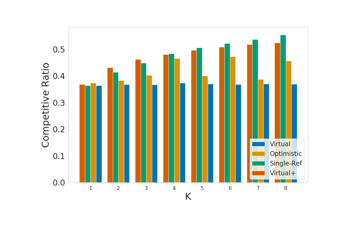
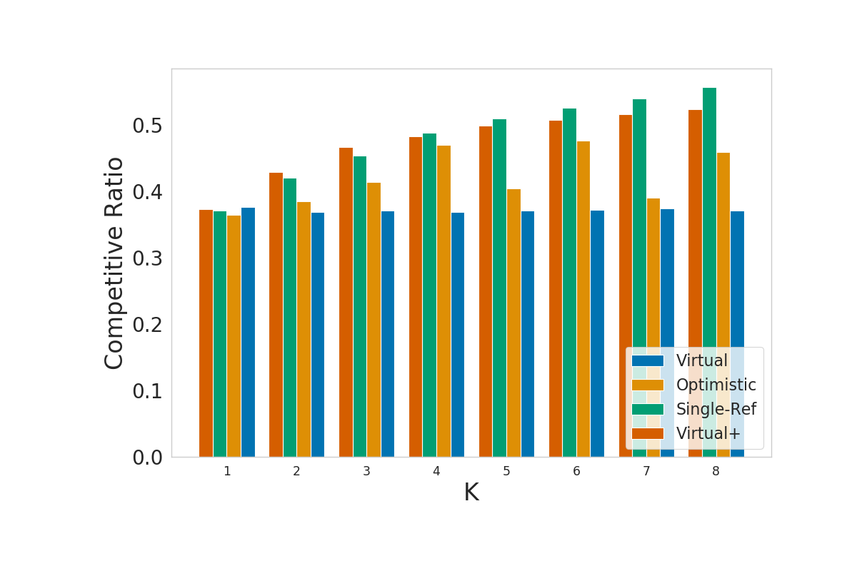
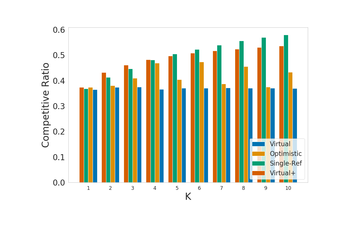
Figure 8: Estimation of the competitive ratio of online algorithms under various noise levels. Left: Deterministic setting with $\sigma^{2}=0$. Middle: Stochastic setting with $\sigma^{2}=1$. Right: Stochastic setting with $\sigma^{2}=5$.

E.3 Experimental Details

We provide more details about the experiments presented in section 5. For further details we also invite the reader to look at the code provided with the supplementary materials. The complete code to reproduce results can be found https://anonymous.4open.science/r/OnlineAttacks-4349

Attack strategies

We use two different attack strategies the Fast Gradient Sign Method (FGSM) (Goodfellow et al., 2015) and 40 iterations of the PGD attack (Madry et al., 2017) with $l_{\infty}$.

Hyper-parameters of online algorithms

All the online algorithms except Single-Ref have a single hyper-parameters to choose which is the length of the sampling phase $t$. For Virtual and Optimistic we use $t=\lfloor\frac{t}{e}\rfloor$ which is the value suggested by theory in Babaioff et al. (2007). For Virtual+ we use $t=\alpha n$ as found by solving the maximization problem for a specific $k$ in Theorem 1. Single-Ref has two hyper-parameters to choose the threshold $t$ ($c$ in the original paper) and reference rank $r$. For $k=1...100$ the values are given in Albers & Ladewig (2020) and are numerical solutions to combinatorial optimization problems. However, for $k=1000$ no values are specified and we choose $c=0.13$ and $r=40$ through grid search. Indeed, these values may not be optimal ones but we leave the choice of better values as future work.

MNIST model architectures

For table 5, $f_{s}$ and $f_{t}$ are chosen randomly from an ensemble of trained classifiers. The ensemble is composed of five different architectures described in table 7, with 5 trained models per architecture.

A	B	C	D
Conv(64, 5, 5) + Relu	Dropout(0.2)	Conv(128, 3, 3) + Tanh	FC(300) + Relu Dropout(0.5)
Conv(64, 5, 5) + Relu	Conv(64, 8, 8) + Relu	MaxPool(2,2)
Dropout(0.25)	Conv(128, 6, 6) + Relu	Conv(64, 3, 3) + Tanh	FC(300) + Relu Dropout(0.5)
FC(128) + Relu	Conv(128, 6, 6) + Relu	MaxPool(2,2)
Dropout(0.5)	Dropout(0.5)	FC(128) + Relu	FC(300) + Relu Dropout(0.5)
FC + Softmax	FC + Softmax	FC + Softmax
			FC(300) + Relu Dropout(0.5)
			FC + Softmax

Table 7: The different MNIST Architectures used for $f_{s}$ and $f_{t}$

CIFAR and Imagenet model architectures

For table 5, $f_{s}$ and $f_{t}$ are chosen randomly from an ensemble of trained classifiers. The ensemble is composed of five different architectures: VGG-16 (Simonyan & Zisserman, 2015), ResNet-18 (RN-18) (He et al., 2016), Wide ResNet (WR) (Zagoruyko & Komodakis, 2016), DenseNet-121 (DN-121) (Huang et al., 2017) and Inception-V3 architectures (Inc-V3) (Szegedy et al., 2016), with 5 trained models per architecture.

E.4 Additional metrics

In addition to the results provided in table 5, we also provide two other metrics here: the stochastic competitive ratio in table 8 and the knapsack ratio table 9. Where the knapsack ratio is defined as the sum value of $S_{\mathcal{A}}$ —i.e. the sum of total loss, as selected by the online algorithm divided by the value of $S^{*}$ selected by the optimal offline algorithm. We observe that the competitive ratio is not always a good metric to compare the actual performance of the different algorithms, since sometimes the online algorithm with the best competitive ratio is not the algorithm with the best fool rate. The knapsack ratio on the other hand seems to be a much better proxy for the actual performance of the algorithms, this is due to the fact that we’re interested in picking elements that have have a good chance to fool the target classifier but are not necessarily the best possible attack.

Table 8: Competitive ratio on non-robust models using FGSM and PGD attacker and various online algorithms.

		MNIST (competitive ratio)			CIFAR-10 (competitive ratio)
	Algorithm	$k=10$	$k=100$	$k=1000$	$k=10$	$k=100$	$k=1000$
FGSM	Naive	.006 $\pm$ .001	.010 $\pm$ .000	.098 $\pm$ .000	.002 $\pm$ .000	.010 $\pm$ .000	.100 $\pm$ .000
	Optimistic	.063 $\pm$ .004	.083 $\pm$ .003	.197 $\pm$ .003	.035 $\pm$ .002	.064 $\pm$ .001	.203 $\pm$ .001
	Virtual	.048 $\pm$ .003	.079 $\pm$ .003	.201 $\pm$ .003	.030 $\pm$ .002	.073 $\pm$ .001	.212 $\pm$ .001
	Single-Ref	.070 $\pm$ .004	.135 $\pm$ .006	.181 $\pm$ .003	.045 $\pm$ .002	.109 $\pm$ .002	.174 $\pm$ .001
	Virtual+	.072 $\pm$ .004	.124 $\pm$ .005	.270 $\pm$ .005	.043 $\pm$ .002	.107 $\pm$ .002	.287 $\pm$ .002
PGD	Naive	.005 $\pm$ .001	.010 $\pm$ .000	.098 $\pm$ .000	.001 $\pm$ .000	.010 $\pm$ .000	.100 $\pm$ .000
	Optimistic	.023 $\pm$ .002	.036 $\pm$ .001	.156 $\pm$ .001	.033 $\pm$ .002	.052 $\pm$ .002	.157 $\pm$ .002
	Virtual	.011 $\pm$ .001	.049 $\pm$ .001	.173 $\pm$ .001	.028 $\pm$ .002	.056 $\pm$ .002	.160 $\pm$ .002
	Single-Ref	.032 $\pm$ .002	.067 $\pm$ .002	.135 $\pm$ .001	.042 $\pm$ .003	.087 $\pm$ .003	.145 $\pm$ .001
	Virtual+	.023 $\pm$ .002	.059 $\pm$ .002	.215 $\pm$ .002	.040 $\pm$ .002	.081 $\pm$ .003	.200 $\pm$ .003

Table 9: Knapsack ratio on non-robust models using FGSM and PGD attacker and various online algorithms.

		MNIST (knapscak ratio in %)			CIFAR-10 (knapsack ratio in %)
	Algorithm	$k=10$	$k=100$	$k=1000$	$k=10$	$k=100$	$k=1000$
FGSM	Naive	19.0 $\pm$ 0.3	19.5 $\pm$ 0.2	29.9 $\pm$ 0.2	16.8 $\pm$ 0.2	20.3 $\pm$ 0.1	28.7 $\pm$ 0.1
	Optimistic	33.0 $\pm$ 0.6	33.1 $\pm$ 0.3	42.1 $\pm$ 0.3	32.7 $\pm$ 0.4	34.1 $\pm$ 0.2	42.8 $\pm$ 0.2
	Virtual	30.8 $\pm$ 0.5	34.2 $\pm$ 0.3	42.9 $\pm$ 0.3	32.9 $\pm$ 0.4	37.8 $\pm$ 0.2	45.0 $\pm$ 0.2
	Single-Ref	39.7 $\pm$ 0.6	41.5 $\pm$ 0.6	40.2 $\pm$ 0.3	37.5 $\pm$ 0.5	45.7 $\pm$ 0.4	37.9 $\pm$ 0.1
	Virtual+	36.2 $\pm$ 0.6	41.1 $\pm$ 0.6	51.4 $\pm$ 0.5	39.4 $\pm$ 0.5	47.1 $\pm$ 0.4	55.5 $\pm$ 0.3
PGD	Naive	27.2 $\pm$ 0.6	15.5 $\pm$ 0.3	25.9 $\pm$ 0.3	22.5 $\pm$ 0.3	26.8 $\pm$ 0.2	36.3 $\pm$ 0.2
	Optimistic	37.2 $\pm$ 0.9	24.2 $\pm$ 0.5	35.8 $\pm$ 0.4	35.3 $\pm$ 0.6	35.6 $\pm$ 0.4	43.1 $\pm$ 0.4
	Virtual	35.6 $\pm$ 0.9	27.5 $\pm$ 0.6	38.8 $\pm$ 0.4	35.5 $\pm$ 0.6	37.2 $\pm$ 0.5	43.9 $\pm$ 0.4
	Single-Ref	46.9 $\pm$ 1.1	34.3 $\pm$ 0.8	32.3 $\pm$ 0.5	39.0 $\pm$ 0.7	42.6 $\pm$ 0.6	41.2 $\pm$ 0.3
	Virtual+	41.5 $\pm$ 1.1	32.3 $\pm$ 0.8	46.5 $\pm$ 0.6	40.9 $\pm$ 0.7	42.9 $\pm$ 0.6	48.8 $\pm$ 0.5

Table 10: Competitive ratio on robust models using FGSM and PGD attacker and various online algorithms.

		MNIST (competitive ratio)			CIFAR-10 (comptetitive ratio)
	Algorithm	$k=10$	$k=100$	$k=1000$	$k=10$	$k=100$	$k=1000$
FGSM	Naive	0.00 $\pm$ 0.00	0.01 $\pm$ 0.00	0.10 $\pm$ 0.00	0.00 $\pm$ 0.00	0.01 $\pm$ 0.00	0.10 $\pm$ 0.00
	Optimistic	0.24 $\pm$ 0.00	0.17 $\pm$ 0.00	0.33 $\pm$ 0.00	0.05 $\pm$ 0.00	0.21 $\pm$ 0.00	0.33 $\pm$ 0.00
	Virtual	0.18 $\pm$ 0.00	0.17 $\pm$ 0.00	0.33 $\pm$ 0.00	0.09 $\pm$ 0.00	0.22 $\pm$ 0.00	0.33 $\pm$ 0.00
	Single-Ref	0.27 $\pm$ 0.00	0.31 $\pm$ 0.00	0.28 $\pm$ 0.00	0.07 $\pm$ 0.00	0.39 $\pm$ 0.00	0.28 $\pm$ 0.00
	Virtual+	0.25 $\pm$ 0.00	0.27 $\pm$ 0.00	0.49 $\pm$ 0.00	0.11 $\pm$ 0.00	0.35 $\pm$ 0.00	0.49 $\pm$ 0.00
PGD	Naive	0.00 $\pm$ 0.00	0.01 $\pm$ 0.00	0.10 $\pm$ 0.00	0.00 $\pm$ 0.00	0.01 $\pm$ 0.00	0.10 $\pm$ 0.00
	Optimistic	0.10 $\pm$ 0.00	0.13 $\pm$ 0.00	0.32 $\pm$ 0.00	0.01 $\pm$ 0.00	0.15 $\pm$ 0.00	0.31 $\pm$ 0.00
	Virtual	0.09 $\pm$ 0.00	0.14 $\pm$ 0.00	0.32 $\pm$ 0.00	0.02 $\pm$ 0.00	0.16 $\pm$ 0.00	0.32 $\pm$ 0.00
	Single-Ref	0.12 $\pm$ 0.00	0.23 $\pm$ 0.00	0.27 $\pm$ 0.00	0.01 $\pm$ 0.00	0.25 $\pm$ 0.00	0.27 $\pm$ 0.00
	Virtual+	0.13 $\pm$ 0.00	0.21 $\pm$ 0.00	0.48 $\pm$ 0.00	0.02 $\pm$ 0.00	0.25 $\pm$ 0.00	0.47 $\pm$ 0.00

Table 11: Knapsack ratio on robust models using FGSM and PGD attacker and various online algorithms.

		MNIST (knapscak ratio in %)			CIFAR-10 (knapsack ratio in %)
	Algorithm	$k=10$	$k=100$	$k=1000$	$k=10$	$k=100$	$k=1000$
FGSM	Naive	1.2 $\pm$ 0.1	2.2 $\pm$ 0.0	10.5 $\pm$ 0.1	9.9 $\pm$ 0.2	12.5 $\pm$ 0.1	19.7 $\pm$ 0.0
	Optimistic	38.0 $\pm$ 0.5	26.5 $\pm$ 0.1	44.6 $\pm$ 0.1	48.8 $\pm$ 0.5	45.2 $\pm$ 0.1	48.3 $\pm$ 0.0
	Virtual	35.6 $\pm$ 0.4	27.0 $\pm$ 0.1	38.0 $\pm$ 0.1	50.9 $\pm$ 0.3	52.5 $\pm$ 0.1	50.0 $\pm$ 0.0
	Single-Ref	46.9 $\pm$ 0.5	45.2 $\pm$ 0.2	46.4 $\pm$ 0.1	59.7 $\pm$ 0.6	73.1 $\pm$ 0.3	41.3 $\pm$ 0.1
	Virtual+	49.2 $\pm$ 0.4	41.2 $\pm$ 0.1	58.6 $\pm$ 0.1	66.2 $\pm$ 0.4	74.5 $\pm$ 0.1	70.5 $\pm$ 0.0
PGD	Naive	1.3 $\pm$ 0.1	2.4 $\pm$ 0.0	10.7 $\pm$ 0.1	11.9 $\pm$ 0.6	14.6 $\pm$ 0.2	21.8 $\pm$ 0.1
	Optimistic	31.1 $\pm$ 0.5	24.4 $\pm$ 0.1	42.7 $\pm$ 0.1	46.0 $\pm$ 1.4	45.3 $\pm$ 0.3	49.2 $\pm$ 0.1
	Virtual	29.9 $\pm$ 0.4	26.3 $\pm$ 0.1	37.9 $\pm$ 0.1	49.4 $\pm$ 1.2	52.4 $\pm$ 0.3	51.6 $\pm$ 0.1
	Single-Ref	39.5 $\pm$ 0.5	41.8 $\pm$ 0.2	43.3 $\pm$ 0.1	56.1 $\pm$ 2.1	69.5 $\pm$ 0.9	42.0 $\pm$ 0.4
	Virtual+	41.3 $\pm$ 0.4	39.7 $\pm$ 0.1	57.9 $\pm$ 0.1	63.4 $\pm$ 1.2	72.7 $\pm$ 0.3	71.2 $\pm$ 0.1

E.5 Additional results

Same architecture

In addition to table 5 we also provide some results on MNIST where $f_{s}$ and $f_{t}$ always have the same architecture but have different weights. This is a slightly less challenging setting as shown in Bose et al. (2020), we also observe that in this setting the adversaries are very effective against the target model.

Table 12: Fool rate on non-robust models, where $f_{s}$ and $f_{t}$ have the same architecture, using FGSM and PGD attacker and various online algorithms.

		MNIST (Fool rate in %)
	Algorithm	$k=10$	$k=100$	$k=1000$
FGSM	Naive (lower bound)	73.5 $\pm$ 0.5	72.3 $\pm$ 0.4	72.6 $\pm$ 0.4
	Opt (Upper-bound)	100.0 $\pm$ 0.0	99.7 $\pm$ 0.0	98.6 $\pm$ 0.1
	Optimistic	89.8 $\pm$ 0.4	86.0 $\pm$ 0.2	84.9 $\pm$ 0.2
	Virtual	90.3 $\pm$ 0.3	90.0 $\pm$ 0.2	88.1 $\pm$ 0.2
	Single-Ref	94.0 $\pm$ 0.3	96.3 $\pm$ 0.2	79.3 $\pm$ 0.3
	Virtual+	96.9 $\pm$ 0.2	98.6 $\pm$ 0.1	97.5 $\pm$ 0.1
PGD	Naive (lower bound)	91.1 $\pm$ 0.5	90.2 $\pm$ 0.4	90.0 $\pm$ 0.3
	Opt (Upper-bound)	98.5 $\pm$ 0.2	98.0 $\pm$ 0.1	97.4 $\pm$ 0.1
	Optimistic	95.3 $\pm$ 0.3	93.8 $\pm$ 0.2	93.5 $\pm$ 0.2
	Virtual	95.5 $\pm$ 0.3	95.2 $\pm$ 0.2	94.4 $\pm$ 0.2
	Single-Ref	96.7 $\pm$ 0.3	96.9 $\pm$ 0.2	92.0 $\pm$ 0.3
	Virtual+	97.1 $\pm$ 0.3	97.6 $\pm$ 0.1	97.0 $\pm$ 0.1

Table 13: Competitive ratio on non-robust models for $k=4$

		MNIST (competitive ratio)	CIFAR (competitive ratio)
	Algorithm	$k=4$	$k=4$
FGSM	Naive	0.004 $\pm$ 0.002	0.002 $\pm$ 0.001
	Optimistic	0.194 $\pm$ 0.016	0.152 $\pm$ 0.012
	Virtual	0.147 $\pm$ 0.013	0.121 $\pm$ 0.011
	Single-Ref	0.200 $\pm$ 0.016	0.160 $\pm$ 0.013
	Virtual+	0.199 $\pm$ 0.016	0.147 $\pm$ 0.012
PGD	Naive	0.001 $\pm$ 0.001	0.000 $\pm$ 0.000
	Optimistic	0.119 $\pm$ 0.013	0.075 $\pm$ 0.021
	Virtual	0.089 $\pm$ 0.010	0.070 $\pm$ 0.019
	Single-Ref	0.119 $\pm$ 0.013	0.059 $\pm$ 0.019
	Virtual+	0.132 $\pm$ 0.013	0.086 $\pm$ 0.022

Table 14: Knapsack ratio on non-robust models for $k=4$

		MNIST (Knapsack ratio in %)	CIFAR (Knapsack ratio in %)
	Algorithm	$k=4$	$k=4$
FGSM	Naive	12.5 $\pm$ 0.3	15.6 $\pm$ 0.3
	Optimistic	34.5 $\pm$ 0.7	36.7 $\pm$ 0.6
	Virtual	31.4 $\pm$ 0.6	33.2 $\pm$ 0.5
	Single-Ref	34.9 $\pm$ 0.7	37.4 $\pm$ 0.6
	Virtual+	37.2 $\pm$ 0.7	38.9 $\pm$ 0.6
PGD	Naive	21.0 $\pm$ 0.6	71.3 $\pm$ 1.6
	Optimistic	39.6 $\pm$ 1.0	82.8 $\pm$ 1.6
	Virtual	35.5 $\pm$ 0.9	81.8 $\pm$ 1.6
	Single-Ref	40.8 $\pm$ 1.0	81.7 $\pm$ 1.5
	Virtual+	42.7 $\pm$ 1.0	84.4 $\pm$ 1.5

Table 15: Fool rate on non-robust models for $k=4$

		MNIST (Fool rate in %)	CIFAR (Fool rate in %)
	Algorithm	$k=4$	$k=4$
FGSM	Naive (lower bound)	59.2 $\pm$ 0.9	59.6 $\pm$ 0.8
	Opt (upper bound)	92.6 $\pm$ 0.5	86.6 $\pm$ 0.6
	Optimistic	83.7 $\pm$ 0.7	79.8 $\pm$ 0.7
	Virtual	80.6 $\pm$ 0.7	76.4 $\pm$ 0.7
	Single-Ref	84.9 $\pm$ 0.7	80.5 $\pm$ 0.7
	Virtual+	86.5 $\pm$ 0.6	82.7 $\pm$ 0.7
PGD	Naive (lower bound)	59.9 $\pm$ 1.2	71.3 $\pm$ 1.6
	Opt (Upper-bound)	79.3 $\pm$ 1.0	87.7 $\pm$ 1.3
	Optimistic	72.1 $\pm$ 1.1	82.8 $\pm$ 1.6
	Virtual	70.0 $\pm$ 1.1	81.8 $\pm$ 1.6
	Single-Ref	74.1 $\pm$ 1.1	81.7 $\pm$ 1.5
	Virtual+	74.5 $\pm$ 1.1	84.4 $\pm$ 1.5

Appendix F Distribution of Values Observed By Online Algorithms

In this section we further investigate performance disparity of online algorithms against robust and non-robust models for CIFAR-10 as observed in Tables 5 and 2. We hypothesize that one possible explanation can be found through analyzing the ratio distribution of values $\mathcal{V}_{i}$’s for unsuccessful and successful attacks as observed by the online algorithm when attacking each model type. However, note that eventhough an online adversary may employ a fixed attack strategy to craft an attack $x^{\prime}=\textsc{ATT}(x)$ the scale of values in each setting are not strictly comparable as the attack is performed on different model types. In other words, given an ATT it is significantly more difficult to attack a robust model and thus we can expect a lower $\mathcal{V}_{i}$ when compared to attacking a non-robust model. Thus to investigate the difference in efficacy of online attacks we pursue a distributional argument.

Indeed, distributions of $\mathcal{V}_{i}$’s observed, for a specific permutation of $\mathcal{D}$, may drastically affect the performance of the online algorithms. Consider for instance, if the $\mathcal{V}_{i}$’s that correspond to successful attacks cannot be distinguished from the ones that are unsuccessful. In such a case one cannot hope to use an online algorithm—that only observes $\mathcal{V}_{i}$’s—to always correctly pick successful attacks. In Figure 9 we visualize the ratio of $\mathcal{V}_{i}$’s of unsuccessful and successful attacks as the ratio of the densities of unsuccessful versus successful attack vectors (y-axis) as provided by a kernel density estimator for CIFAR-10 robust and non-robust models. It provides a non-normalized value of the ratio of unsuccessful attacks for a given value of $\mathcal{V}_{i}$. As observed, there is a significant amount of non-successful attacks for large values of $\mathcal{V}_{i}$ in the non-robust case which indicates that there are many data points with high values that lead to unsuccessful attacks. Furthermore, this also suggests one explanation for the higher efficacy of online algorithms against robust models: fewer attacks are successful but they are easier to differentiate from unsuccessful ones because of their relatively larger loss value. Importantly, this implies that given an online attack budget $k\ll n$ higher online fool rates can be achieved against robust models as the selected data points turn adversarial with higher probability when compared to non-robust models.

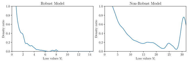
Figure 9: Distribution of the values for robust and non-robust models. We use a gaussian kernel density estimator to estimate the density.

Appendix G Related Work

Adversarial attacks. The idea of attacking deep networks was first introduced in (Szegedy et al., 2014; Goodfellow et al., 2015), and recent years have witnessed the introduction of challenging threat models, such as blackbox Chen et al. (2017); Ilyas et al. (2018); Jiang et al. (2019); Bose et al. (2020); Chakraborty et al. (2018) as well as defense strategies Madry et al. (2017); Tramèr et al. (2018); Ding et al. (2020). Closest to our setting are adversarial attacks against real-time systems Gong et al. (2019a; b) and deep reinforcement learning agents Lin et al. (2017); Sun et al. (2020). However, unlike our work, these are not online algorithms and do not impose online constraints (see §G).

$k$-secretary. The classical secretary problem was originally proposed by Gardner (1960) and later solved in Dynkin (1963) with an $(1/e)$-optimal algorithm. Kleinberg (2005) introduced the $k$-secretary problem and an asymptotically optimal algorithm achieving a competitive ratio of $1-\Theta(\sqrt{1/k})$. As outlined in §1 for general $k$ an optimal algorithms exist Chan et al. (2014), but requires the analysis of involved LPs that grow with the size of $n$. A parallel line of work dubbed the prophet secretary problem, considers online problems where—unlike §4.1—some information on the distribution of values is known a priori Azar et al. (2014; 2018); Esfandiari et al. (2017). Secretary problems have also been applied to machine learning by informing the online algorithm about the inputs before execution Antoniadis et al. (2020); Dütting et al. (2020). Finally, other interesting secretary settings include playing with adversaries Bradac et al. (2020); Kaplan et al. (2020).

While we consider —to the best of our knowledge—that our work is the only truly online threat model. Our setting is the only one considering that data points are only ever observed once, and a decision to attack must be made at the moment and cannot be reversed retroactively. For example, (Gong et al., 2019b) consider replay attacks on Voice-Controlled Systems whereby streamed audio input is captured with a recording device, and then the entire sequence is spoofed and replayed back. Unlike online attacks that we consider, they can manipulate the whole sequence retroactively and do not have to make an irreversible decision to attack at a given timestep. Similarly, both (Lin et al., 2017; Sun et al., 2020) consider adversarial attacks against deep reinforcement learning agents. Like us, they consider an adversarial budget that limits the number of points to attack to avoid detection. However, unlike us, they require whitebox access to the target model in order to train another predictive model by interacting with the environment, which can later be used to inform “when to attack”. Thus the datapoints appearing at test time may already be seen and scored during the training period. The dichotomy between collecting data for potentially an infinite time horizon before attacking is at odds with our online threat model as a data point can only be observed once. As a result, none of these works can be used within our online threat model and are not appropriate baselines.

References

- Akhtar & Mian (2018) Naveed Akhtar and Ajmal Mian. Threat of adversarial attacks on deep learning in computer vision: A survey. IEEE Access, 2018.
- Albers & Ladewig (2020) Susanne Albers and Leon Ladewig. New results for the -secretary problem. arXiv preprint arXiv:2012.00488, 2020.
- Antoniadis et al. (2020) Antonios Antoniadis, Themis Gouleakis, Pieter Kleer, and Pavel Kolev. Secretary and online matching problems with machine learned advice. arXiv preprint arXiv:2006.01026, 2020.
- Azar et al. (2014) Pablo D Azar, Robert Kleinberg, and S Matthew Weinberg. Prophet inequalities with limited information. In Proceedings of the twenty-fifth annual ACM-SIAM symposium on Discrete algorithms. SIAM, 2014.
- Azar et al. (2018) Yossi Azar, Ashish Chiplunkar, and Haim Kaplan. Prophet secretary: Surpassing the 1-1/e barrier. In Proceedings of the 2018 ACM Conference on Economics and Computation, 2018.
- Babaioff et al. (2007) Moshe Babaioff, Nicole Immorlica, David Kempe, and Robert Kleinberg. A knapsack secretary problem with applications. In Approximation, randomization, and combinatorial optimization. Algorithms and techniques. Springer, 2007.
- Bose et al. (2020) Avishek Joey Bose, Gauthier Gidel, Hugo Berard, Andre Cianflone, Pascal Vincent, Simon Lacoste-Julien, and William L Hamilton. Adversarial example games. Thirty-fourth Conference on Neural Information Processing Systems, 2020.
- Bradac et al. (2020) Domagoj Bradac, Anupam Gupta, Sahil Singla, and Goran Zuzic. Robust Algorithms for the Secretary Problem. In ITCS, 2020.
- Buchbinder et al. (2014) Niv Buchbinder, Kamal Jain, and Mohit Singh. Secretary problems via linear programming. Mathematics of Operations Research, 39(1):190–206, 2014.
- Carlini & Wagner (2017) Nicholas Carlini and David Wagner. Magnet and efficient defenses against adversarial attacks are not robust to adversarial examples. arXiv preprint arXiv:1711.08478, 2017.
- Chakraborty et al. (2018) Anirban Chakraborty, Manaar Alam, Vishal Dey, Anupam Chattopadhyay, and Debdeep Mukhopadhyay. Adversarial attacks and defences: A survey. arXiv preprint arXiv:1810.00069, 2018.
- Chan et al. (2014) TH Hubert Chan, Fei Chen, and Shaofeng H-C Jiang. Revealing optimal thresholds for generalized secretary problem via continuous lp: impacts on online k-item auction and bipartite k-matching with random arrival order. In Proceedings of the Twenty-Sixth Annual ACM-SIAM Symposium on Discrete Algorithms, 2014.
- Chen et al. (2017) Pin-Yu Chen, Huan Zhang, Yash Sharma, Jinfeng Yi, and Cho-Jui Hsieh. Zoo: Zeroth order optimization based black-box attacks to deep neural networks without training substitute models. In Proceedings of the tenth ACM Workshop on Artificial Intelligence and Security. ACM, 2017.
- Chen et al. (2020) Steven Chen, Nicholas Carlini, and David Wagner. Stateful detection of black-box adversarial attacks. In Proceedings of the 1st ACM Workshop on Security and Privacy on Artificial Intelligence, pp. 30–39, 2020.
- Ding et al. (2020) Gavin Weiguang Ding, Yash Sharma, Kry Yik Chau Lui, and Ruitong Huang. MMA training: Direct input space margin maximization through adversarial training. In International Conference on Learning Representations, 2020.
- Dütting et al. (2020) Paul Dütting, Silvio Lattanzi, Renato Paes Leme, and Sergei Vassilvitskii. Secretaries with advice. arXiv preprint arXiv:2011.06726, 2020.
- Dynkin (1963) Evgenii Borisovich Dynkin. The optimum choice of the instant for stopping a markov process. Soviet Mathematics, 1963.
- Esfandiari et al. (2017) Hossein Esfandiari, MohammadTaghi Hajiaghayi, Vahid Liaghat, and Morteza Monemizadeh. Prophet secretary. SIAM Journal on Discrete Mathematics, 2017.
- Ferguson et al. (1989) Thomas S Ferguson et al. Who solved the secretary problem? Statistical science, 1989.
- Gardner (1960) Martin Gardner. Mathematical games. Scientific American, 1960.
- Gong et al. (2019a) Yuan Gong, Boyang Li, Christian Poellabauer, and Yiyu Shi. Real-time adversarial attacks. Proceedings of the Twenty-Eighth International Joint Conference on Artificial Intelligence IJCAI-19, 2019a.
- Gong et al. (2019b) Yuan Gong, Jian Yang, Jacob Huber, Mitchell MacKnight, and Christian Poellabauer. ReMASC: Realistic Replay Attack Corpus for Voice Controlled Systems. In Proc. Interspeech 2019, 2019b.
- Goodfellow et al. (2015) Ian J Goodfellow, Jonathon Shlens, and Christian Szegedy. Explaining and harnessing adversarial examples. Third International Conference of Learning Representations (ICLR), 2015.
- He et al. (2016) Kaiming He, Xiangyu Zhang, Shaoqing Ren, and Jian Sun. Deep residual learning for image recognition. In Proceedings of the IEEE conference on computer vision and pattern recognition, 2016.
- Huang et al. (2017) Gao Huang, Zhuang Liu, Laurens Van Der Maaten, and Kilian Q Weinberger. Densely connected convolutional networks. In Proceedings of the IEEE conference on computer vision and pattern recognition, pp. 4700–4708, 2017.
- Ilyas et al. (2018) Andrew Ilyas, Logan Engstrom, Anish Athalye, and Jessy Lin. Black-box adversarial attacks with limited queries and information. Thirty-fifth International Conference on Machine Learning (ICML), 2018.
- Ilyas et al. (2019) Andrew Ilyas, Logan Engstrom, Anish Athalye, and Jessy Lin. Query-efficient black-box adversarial examples. In ICLR, 2019.
- Jiang et al. (2019) Linxi Jiang, Xingjun Ma, Shaoxiang Chen, James Bailey, and Yu-Gang Jiang. Black-box adversarial attacks on video recognition models. In Proceedings of the twenty-seventh ACM International Conference on Multimedia, 2019.
- Kaplan et al. (2020) Haim Kaplan, David Naori, and Danny Raz. Competitive analysis with a sample and the secretary problem. In Proceedings of the Fourteenth Annual ACM-SIAM Symposium on Discrete Algorithms. SIAM, 2020.
- Kleinberg (2005) Robert D Kleinberg. A multiple-choice secretary algorithm with applications to online auctions. In SODA, 2005.
- Krizhevsky (2009) Alex Krizhevsky. Learning multiple layers of features from tiny images. In Tech Report, UofT, 2009.
- LeCun & Cortes (2010) Yann LeCun and Corinna Cortes. MNIST handwritten digit database. 2010. URL http://yann.lecun.com/exdb/mnist/.
- Lin et al. (2017) Yen-Chen Lin, Zhang-Wei Hong, Yuan-Hong Liao, Meng-Li Shih, Ming-Yu Liu, and Min Sun. Tactics of adversarial attack on deep reinforcement learning agents. In Proceedings of the Twenty-Sixth International Joint Conference on Artificial Intelligence, IJCAI-17, 2017.
- Madry et al. (2017) Aleksander Madry, Aleksandar Makelov, Ludwig Schmidt, Dimitris Tsipras, and Adrian Vladu. Towards deep learning models resistant to adversarial attacks. Sixth International Conference on Learning Representations (ICLR), 2017.
- Papernot et al. (2016) Nicolas Papernot, Patrick McDaniel, and Ian Goodfellow. Transferability in machine learning: from phenomena to black-box attacks using adversarial samples. arXiv preprint arXiv:1605.07277, 2016.
- Papernot et al. (2017) Nicolas Papernot, Patrick McDaniel, Ian Goodfellow, Somesh Jha, Z Berkay Celik, and Ananthram Swami. Practical black-box attacks against machine learning. In Proceedings of the 2017 ACM on Asia Conference on Computer and Communications Security. ACM, 2017.
- Simonyan & Zisserman (2015) Karen Simonyan and Andrew Zisserman. Very deep convolutional networks for large-scale image recognition. Third International Conference on Learning Representations (ICLR), 2015.
- Sun et al. (2020) Jianwen Sun, Tianwei Zhang, Xiaofei Xie, Lei Ma, Yan Zheng, Kangjie Chen, and Yang Liu. Stealthy and efficient adversarial attacks against deep reinforcement learning. The Thirty-Fourth AAAI Conference on Artificial Intelligence (AAAI-20), 2020.
- Szegedy et al. (2014) Christian Szegedy, Wojciech Zaremba, Ilya Sutskever, Joan Bruna, Dumitru Erhan, Ian Goodfellow, and Rob Fergus. Intriguing properties of neural networks. Second International Conference on Learning Representations (ICLR), 2014.
- Szegedy et al. (2016) Christian Szegedy, Vincent Vanhoucke, Sergey Ioffe, Jon Shlens, and Zbigniew Wojna. Rethinking the inception architecture for computer vision. In Proceedings of the IEEE conference on computer vision and pattern recognition, pp. 2818–2826, 2016.
- Tramèr et al. (2017) Florian Tramèr, Nicolas Papernot, Ian Goodfellow, Dan Boneh, and Patrick McDaniel. The space of transferable adversarial examples. arXiv preprint arXiv:1704.03453, 2017.
- Tramèr et al. (2018) Florian Tramèr, Alexey Kurakin, Nicolas Papernot, Ian Goodfellow, Dan Boneh, and Patrick McDaniel. Ensemble adversarial training: Attacks and defenses. Sixth International Conference on Learning Representations (ICLR), 2018.
- Zagoruyko & Komodakis (2016) Sergey Zagoruyko and Nikos Komodakis. Wide residual networks. In British Machine Vision Conference 2016. British Machine Vision Association, 2016.