Current address:]Department of Bioengineering, School of Engineering & Applied Science, University of Pennsylvania, Philadelphia, PA 19104, USA

Topological Design of Heterogeneous Self-Assembly

Abstract

Controlling the topology of structures self-assembled from a set of heterogeneous building blocks is highly desirable for many applications, but is poorly understood theoretically. Here we show that the thermodynamic theory of self-assembly involves an inevitable divergence in chemical potential. The divergence and its detailed structure are controlled by the spectrum of the transfer matrix, which summarizes all of self-assembly design degrees of freedom. By analyzing the transfer matrix, we map out the phase boundary between the designable structures and the unstructured aggregates, driven by the level of cross-talk.

Self-assembly is an robust method for organizing loose building blocks to adopt desired structures[1]. A wide range of structures has been observed in synthetic self-assembly in both experiments and numerical simulations, from strictly periodic crystals [2] to quasicrystals [3], liquid crystals [4], polymers [5], nets [6], and finite clusters [7]. While initial investigations were guided by anecdotal evidence and limited availability of building blocks, later works deliberately optimize building block properties to assemble a desired target structure [8]. The emergent connection between building block properties and the structures they form makes self-assembly a model system for discussion of more general design principles [9].

A great challenge in self-assembly design is controlling the topology of target structures (Fig. 1a). Topologically closed structures, such as 2D rings and 3D spheres [10, 11], have important applications in functional foods [12], biomedicine [13], and drug delivery [14], and it is natural to ask how this can be encoded into interactions between components. The competition between open and closed structures at finite concentration is naturally described by grand canonical thermodynamic theory. However, such a theory has an inevitable divergence in the chemical potential. In this paper, we use this divergence as a design tool to encode self assembled structure. We use this to make quantitative predictions of self-assembly yields of linear chains and closed rings for arbitrary binding energy matrices, and then use this to derive qualitative and quantitative design rules for optimal binding energy matrices. This allows predicting the limits on complexity of structures driven by interaction cross-talk. This theoretical framework accounts for a whole set of building blocks, and thus opens the design of even more complex, higher-dimensional, branching, and loopy structures.

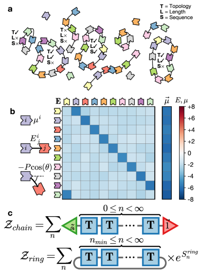
Figure 1: The design space of the heterogeneous self-assembly problem. (a) Self-assembled structures vary by topology (T), length (L), and sequence (S). Check and cross marks indicate whether the structures match the target (here, a length 10 ring). (b) The set of building blocks is characterized by their chemical potentials $\mu^{i}$, key-lock binding energies $E^{i}_{\;j}$, and bending rigidity $P$. The on-target binding energies are very negative (dark blue), while the off-target binding energies are only slightly negative (light blue). (c) Computations of partition functions for linear chains and closed rings in graphical (tensor) notation, corresponding to Eqns. (2–3).

In order to self-assemble target structures, we seek to jointly design a set of $N$ building blocks, where each building block has a “lock” and “key” binding site on opposite sides. Binding occurs between the locks and keys of different particles. Lock and key interactions have been experimentally realized [15, 16, 17] but for the present investigation we abstract specific realizations. The set of building blocks is then described by the chemical potential concentration vector $\vec{\mu}$, the binding energy matrix $\mathbf{E}$, and the bond rigidity $P$ (see Fig. 1b).

Building block interaction is controlled by the binding energy. We denote the binding energy between the key side of particle $i$ and the lock side of particle $j$ as $E^{i}_{\;j}$, with indices $i,j$ spanning the range $[1,N]$; the entries form a matrix $\mathbf{E}$ (see Fig. 1b). To design $\mathbf{E}$, we designate certain $(i,j)$ pairs as on-target, by making the corresponding binding energies stronger (more negative) $\absolutevalue{E_{\textsf{on-target}}}\gg\absolutevalue{E_{\textsf{off-target}}}$.

Even with designed interactions, off target binding is ubiquous in every practical experimental system, including DNA origami [18], DNA-coated colloids [19], de novo proteins [20], and magnetic panels [6]. This means we cannot control all of the entries of $\mathbf{E}$ independently: adding an interaction patch with a specific on-target partner requires addding the off-target bindings as well. Off-target interactions limit the effective number of distinct building blocks in the system and thus the yield of complex self-assembled structures [21, 22]. In this paper we study how off-target binding specifically limits our ability to control topology via the binding energy matrix, with the bond rigidity and the relative concentrations of building blocks serving as secondary parameters [22].

To proceed, we construct the transfer matrix $\mathbf{T}$, which is defined element-wise following Ref. [22]:

$$T^{i}_{\;j}=\exp(\beta(-E^{i}_{\;j}+\mu^{j})+S_{b}).$$ (1)

The transfer matrix corresponds to adding one more element to the chain of building blocks. The first index $i$ accounts for the possible key binding sites exposed by the preceding part of the chain, while the second index $j$ accounts for binding to locks. This definition of the transfer matrix closely follows that used in solving spin lattice models [23], with the chemical potential playing the role of external field. It is also very similar to the coupling tensors in Refs. [24, 25]. In the present problem, the topology of interactions is simple, so the matrix product and tensor contraction views are equivalent. In what follows, we use this tensor perspective to compute the partition functions for all possible chains and rings (see Appendix A for a full derivation). The expressions are presented in a graphical tensor form in Fig. 1c, but can also be written down analytically in closed form:

$$\mathcal{Z}_{chain} =\underaccent{\vec}{z}\mathbf{D}\vec{1}$$ (2)

$$\mathcal{Z}_{ring} =\frac{1}{(2\pi\xi)^{3/2}}\left(\Tr(\operatorname{Li}_{3/2}(\mathbf{T}))-\sum\limits_{n=1}^{n_{min}-1}\frac{\Tr(\mathbf{T}^{n})}{n^{3/2}}\right),$$ (3)

where $\mathbf{D}\equiv\left(\mathbf{I}-\mathbf{T}\right)^{-1}$ is the propagator, or sum of a matrix geometric series, $\operatorname{Li}_{q}(x)$ is the $q$-order polylogarithm function generalized to matrix arguments, and $\xi$ is the persistence length of the polymer chain, related to its rigidity $P$. The key difference between the two expressions is that self-assembly of closed rings requires paying a hefty entropic loop penalty so that the end of the closed chain is co-located with the beginning [26]. This penalty significantly reduces the assembly rate of the rings.

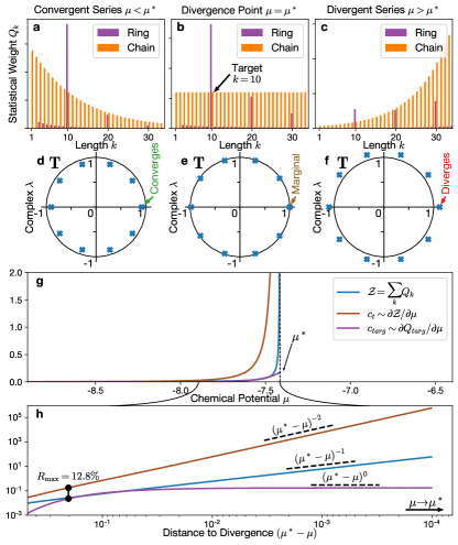
Figure 2: Design of self-assembling clusters needs to hide structure in nearly-divergent series. (a,b,c) Sequences of statistical weights $Q_{k}$ in a system designed well to assemble rings of length $k=10$, at different $\mu$. (d,e,f) Complex eigenvalue spectra of the corresponding transfer matrices $\mathbf{T}$, with the top eigenvalue $\lambda_{0}$ determining the divergence. (g) Graph of partition function $\mathcal{Z}$, total concentration $c_{t}$, and target concentration $c_{targ}$ against the chemical potential $\mu$ in linear axis scales. The point labeled $\mu^{*}$ indicates the divergence. (h) Graph of the same quantities as (g) but in log-log axis scales in vicinity of $\mu^{*}$. Dashed lines guide the eye for different power law divergence scaling. Maximal conversion ratio $R_{\max}$ is achieved at finite distance from the divergence.

The expressions (2)-(3) have a form specific to our building blocks. More generically, the combinatorial partition function of any sticky particle model takes the form of an infinite series of statistical weights $Q_{s}$ of all possible structures $s$:

$$\mathcal{Z}=\sum\limits_{s}\exp(\beta\left(\underaccent{\vec}{n}_{s}\cdot\vec{\mu}-E_{s}\right)+S_{s}),$$ (4)

where $\underaccent{\vec}{n}_{s}$ is the vector of numbers of particles of each type in the structure $s$, $E_{s}$ is the energy of all bonds, and $S_{s}$ is the internal entropy of the cluster due to vibrations and rotations. The sum over cluster types $s$ typically has an infinite number of terms with ever increasing particle counts $\underaccent{\vec}{n}_{s}$. Although there is a parameter regime where this infinite sum converges, since the chemical potentials $\vec{\mu}$ are free parameters, we can always make them arbitrarily high, rendering the series divergent. While such a divergence is generic for all partition functions with an infinite number of terms, the exact value of ${\mu^{i}}^{*}$ at which the divergence occurs, as well as the behavior of the partition function close to the divergence is model-specific.

For the specific building block model discussed here, the typical sequences of statistical weights $Q_{k}$ in terms of structure length $k$ are illustrated in Fig. 2a-c. Depending on the chemical potential $\mu$, the series can either converge (panel a), diverge (panel c), or be exactly at the margin (panel b). Since the partition functions for chains and rings (2)-(3) are computed as infinite series in matrices, their convergence is determined by the eigenvalue spectrum of the transfer matrix $\mathbf{T}$. While the eigenvalues are generally complex, the top eigenvalue $\lambda_{0}$ is guaranteed to be real by the Perron-Frobenius theorem. The partition function converges when $\lambda_{0}<1$ (panel d of Fig. 2), diverges for $\lambda_{0}>1$ (panel f), and switches between the two regimes at $\lambda_{0}=1$ (panel e).

Is this divergence a physically observable phenomenon or a phase transition? The divergence occurs under variation of the chemical potential $\mu$, directly related to the concentration of free (unbound) building blocks $c_{free}=c_{0}e^{\beta\mu}$. In experiments we do not control the free concentration, but the total concentration $c_{t}$ of building blocks. In particular, we can take derivatives of the partition functions (2)–(3) with respect to $\mu$ and compute similar, albeit bulkier, closed form expressions for the concentrations of building blocks bound in all structures $c_{t}$, or only in the desired target structure $c_{targ}$. We present the values of $\mathcal{Z}$,$c_{t}$,$c_{targ}$ in Fig. 2g-h, first in linear scale to emphasize the divergence, and then in log-log scale to emphasize the scaling.

In vicinity of the divergence, the lead eigenvalue scales as $\lambda_{0}\simeq e^{\beta(\mu-\mu^{*})}$, dominating the partition function, and determining the divergence exponents for both the partition functions and the total concentrations (Fig. 2g-h). We find that the total concentrations of building blocks bound in chains and in rings have the same divergence point $\mu^{*}$ but different asymptotic behaviors [27]:

$$c_{chain} \sim(\mu^{*}-\mu)^{-2}$$ (5)

$$c_{ring} \sim(\mu^{*}-\mu)^{-1/2}.$$ (6)

These expressions demonstrate that arbitrarily close to the divergence, i.e. at high concentrations, many more building blocks are bound chains than in rings, regardless of our design efforts. Moreover, we find that near the divergence, the total concentrations are dominated by arbitrarily long chains and rings, longer than any finite target we might choose. Therefore, the highest conversion ratio of raw monomers into the designed finite-size targets always occurs a finite distance from the divergence point. To quantify this in what follows, we use the ratio $R\equiv c_{targ}/c_{t}$ .

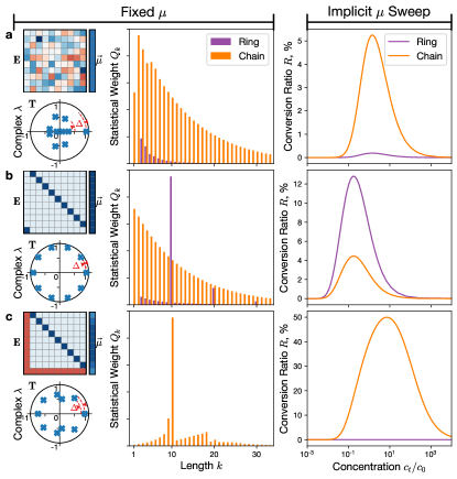
Figure 3: Examples of yield predictions for several building block set designs. Columns of panels show different metrics, rows show different designs. Columns: (left-top) Binding energy matrix $\mathbf{E}$ and chemical potential vector $\vec{\mu}$. (left-bottom) Complex spectrum of the corresponding transfer matrix $\mathbf{T}$. Red arcs indicate the spectral gap $\Delta$ between the first and second eigenvalues. (center) Statistical weight $Q_{k}$ sequences. (right) Conversion ratio of raw monomers into the target structure, summed over all monomer types, plotted as a parametric curve with implicit parameter $\mu$. Rows: (a) Random unstructured binding energy matrix. (b) Binding energy matrix designed for assembly of rings of length $k=10$. (c) Binding energy matrix and the chemical potential profile designed for assembly of chains of length $k=10$.

Fig. 3 shows how to work around this divergence and make testable experimental predictions. We first design the binding energy matrix $\mathbf{E}$ and the chemical potential profile $\Delta\mu$ at fixed $\mu$ and study the eigenvalue spectrum of $\mathbf{T}$ and the sequence of $Q_{k}$ (left part of figure). We then sweep over $\mu$ as an implicit parameter, compute $c_{t}(\mu)$ and $R(\mu)$ and plot them against each other (right part of figure, see Appendix A for details).

To unravel the connection between design space and self-assembly yields, we use the analytic expressions to explore several specific design scenarios. In all three cases we study a set of $N=10$ building block types and focus on the yields of structures of length $k=10$, both chains and rings. We choose the value of correlation length $\xi=1$. We keep $\beta=1$ and vary the binding energy matrix to explore three design scenarios shown in Fig. 3.

Fig. 3a shows a random binding energy matrix $\mathbf{E}$. This occurs in practice when “on-target” and “off-target” bindings are effectively indistinguishable. The sequence of statistical weights $Q_{k}$ then closely resembles a simple unstructured geometric series. This does not mean that clusters do not form – instead, the formed clusters can be large but don’t have any particular structure. This is a failure state of design, generically observed when off-target interactions are strong.

Fig. 3b shows a binding energy matrix $\mathbf{E}$ designed for forming closed rings. The key of each building block $i$ has strong on-target binding to the next lock $i+1$, with the last one binding to the first in a cyclical fashion. In the graphical representation of the matrix, this is visible as a dark first superdiagonal and an opposite corner element. The complex spectrum for this scenario shows a very small spectral gap $\Delta$, which as we show below is a strong predictor and a requirement of forming rings of precise sequence. In the sequence of statistical weights this design causes a strong peak for $k=10$ rings and smaller ones for $k=20$ and $k=30$ (when the full ring sequence is repeated multiple times). This design also shows a substantial $R\approx 12\%$ for the rings despite them being fundamentally disadvantaged by the loop entropy penalty.

Fig. 3c shows a system of binding energy matrix $\mathbf{E}$ and chemical potential vector $\vec{\mu}$ designed for forming finite chains. In the binding energy matrix $\mathbf{E}$, the left column and the bottom row are red (positive, repulsive), corresponding to the removed lock binding site on the first building block and key binding site on the last one. In the chemical potential vector, the entries for the first and last building blocks are substantially larger than the ones in the middle of the vector following Ref. [22]. As a result, in the sequence of statistical weights $k=10$ is much larger than any of the other ones. Almost $R\approx 50\%$ of building blocks are converted into length 10 chains.

The designs presented in Fig. 3 are intuitive guesses, picked for illustrative purposes. Any real system of heterogeneous building blocks is highly constrained by the off-target binding energy, limiting the size of structures that can be reliably self-assembled. For any self-assembly theory to be useful in practice, the design rules must be not just qualitative, but quantitative. The design rules for open chains have been studied previously in Ref. [22], so here we focus on the design rules for closed rings and derive the limits on structure size set by cross-talk. We consider cyclic binding matrices of form shown in Fig. 3b with variable on-target $v$ and off-target $\epsilon$ binding energies such that $v<\epsilon<0$.

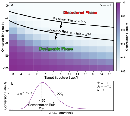
Figure 4: Design rules for self-assembly of closed rings. (a) Heatmap of conversion ratio $R$, maximized over the implicit chemical potential $\mu$. Horizontal axis is the number of building block types, equal to the target structure size. Vertical axis is the strength of on-target binding $\beta v$ with off-target binding fixed at $\beta\epsilon=-1$. Black curves illustrate the precision and boundary design rules, which separate the amyloid and the designable phases. (b) Typical curve of conversion ratio $R$ against the total concentration $c_{t}$. The curve maximum lies around the estimated value $c_{opt}$, and the logarithmic width of the high-yield regime is around $e^{4}\simeq 50$ fold. The shapes of left and right curve tails have different asymptotic behaviors, as indicated.

Our results suggest a series of design rules: First, the precision rule ensures that the building blocks assemble the proper linear sequence. When this occurs, the weight $Q_{k}$ is significantly boosted for $k=N$ (see Appendix B for derivation). This boost is significant when the eigengap $\Delta=\absolutevalue{\lambda_{0}}-\absolutevalue{\lambda_{1}}$ is sufficiently small. This is achieved when on-target binding overcomes the many possible off-target bindings:

$$\beta(v-\epsilon)\ll-\ln(\frac{N^{2}}{\ln N}).$$ (7)

This design rule is qualitatively similar though slightly more stringent than the “$\ln N$ rule” for linear chains derived in Ref. [22]. If this constraint on the binding energy contrast $\epsilon-v$ is not observed, the assembled chains will have random sequences (Fig. 3a), and controlling any higher-level structure would become impossible.

The second design rule is the boundary rule, ensuring that the last building block in the ring sequence binds to the first one. For this to occur, the binding energy needs to be strong enough to overcome the ring entropy penalty. Assuming the boundary rule (7) holds, we derive the following, stronger condition:

$$\beta v\ll S_{b}-\frac{3}{2}\ln(2\pi\xi)-\frac{3}{2}\ln(N)-\frac{e^{-\beta\epsilon}}{(2\pi\xi)^{3/2}}N^{1/2}.$$ (8)

Since longer chains experience higher entropy penalty, their reliable assembly requires somewhat stronger on-target binding, following a $N^{1/2}$ power law rather than $\ln N$ rule.

The third design rule is the concentration rule, which establishes the finite interval of total building block concentrations that are optimally converted into the target structure. The upper and lower limits of this interval have different physical origins. At the upper limit, the absolute concentration of building blocks in the target structure $c_{targ}$ is not singular at $\mu^{*}$ (Fig. 2g-h). However, the total concentration of building blocks in all structures keeps growing, thus the conversion ratio drops off as $R\propto 1/c_{t}$. At the lower limit, the conversion ratio is driven by $c_{targ}\propto e^{-1/\sqrt{c_{t}}}$ (see Appendix C for discussion of concentration units [28]). Balancing the two effects results in the maximal conversion ratio at an intermediate optimal concentration:

$$e^{-2}<\frac{c_{t}}{c_{opt}}<e^{2};\quad c_{opt}=c_{0}\frac{N^{3}}{4}e^{\beta v-S_{b}},$$ (9)

where the lower and upper limits correspond to decrease of $R$ by a factor of $e$. The full width of the high-yield concentration range is $e^{4}\simeq 50$.

We test the three design rules by comparing the analytic limits with numerical computations of $R$ for a range of on-target bindings $\beta v$ and target structure sizes $N$ in Fig. 4. As expected, significant conversion ratio is only achieved for parts of the $(N,\beta v)$ plane significantly below both the precision and boundary rules (7)–(8), with the second one providing a tighter bound (panel a). The concentration rule accurately estimates the location and width of the $R$ maximum (panel b).

In this paper we investigate theoretically how to control the topology of structures self-assembled from heterogeneous building blocks, focusing on the central divergence in the partition function for both ordered and disordered binding energy matrices. By mitigating this divergence, we predict the quantitative boundary between designable and the intrinsically disordered regions of the design space [29]. This framework opens the way to further quantitative investigations of formation of amyloids and design of structures of more complex topologies.

Appendix A Combinatorial theory

This section details the computation of the cluster partition function (73) for our specific model system. We first introduce the hierarchical sum of the partition function over the topologies, lengths, and sequences. We then define the transfer matrix as the central element of the combinatorial calculation. We derive closed-form partition functions for linear chains and rings and indicate their convergence criteria. We show how the convergence and other properties of the partition function relate to the spectral properties of the transfer matrix. As we approach the divergence point, the chain and ring partition functions diverge at different rates, thus informing the entropic trade-off between them. We conclude the section with deriving the total concentrations and absolute yields of building blocks in closed form.

In order to start computing the partition functions, we need to look back at the hierarchical taxonomy of structures that can be assembled . The structure index $s$ so far did not refer to this hierarchy and was treated as one-dimensional. Without invalidating any of the summations in $s$, we can use it to refer to the topology, the length, and the specific sequence of the structure. In this case we can write the cluster partition function as a triple sum:

$$\mathcal{Z}_{cl}=\sum\limits_{\textsf{topology}}\sum\limits_{\textsf{length}}\sum\limits_{\textsf{sequence}}Q_{s}.$$ (10)

The outermost sum is over the possible topologies. As we stated before, the monomers with two binding sites can only assemble two different topologies: chains and rings. For these topologies, we will write down two different expressions and add them up. The sum in length is relatively straightforward since the structures are one-dimensional, so the possible lengths are enumerated by a single set of natural numbers with some starting point. The sum in possible sequences is more tricky. However, since the energies of bonds and chemical potentials of the monomers are additive, the corresponding statistical weights are multiplicative and can be expressed via matrix products by following the approach of Ref. [22]. The following sections derive the partition function expressions from the bottom up and develop the tools for their analysis.

A.1 Chain and ring partition functions

A linear chain consists of three components: the initial monomer driven only by the chemical potential, some number of subsequent monomers described by the transfer matrix, and the interaction of the last monomer with the solvent. The selection of the initial monomer is given by the vector of fugacities $\underaccent{\vec}{z}:z_{i}\equiv e^{\beta\mu^{i}}$. The number of intervening monomers varies between zero and infinity and is accounted by the sum in length. The terminus is taken as $\vec{1}$, a vector of all 1’s since we assume that monomers don’t have any specific interactions with the solvent. In this case, the partition function of all possible chains is given by:

$$\mathcal{Z}_{chain}=\sum\limits_{n=0}^{\infty}\underaccent{\vec}{z}\mathbf{T}^{n}\vec{1}.$$ (11)

Note that for each term $n$, the chain has $n$ bonds that contribute energy and entropy and $n+1$ monomers that contribute the chemical potential. The contraction of the transfer matrix with the fugacities on the left and the terminus on the right can be taken outside of the summation due to linearity. The internal sum is then a simple geometric series in the matrix $\mathbf{T}$ that we will call the propagator $\mathbf{D}$:

$$\mathbf{D}\equiv\sum\limits_{n=0}^{\infty}\mathbf{T}^{n}=\left(\mathbf{I}-\mathbf{T}\right)^{-1},$$ (12)

where $\mathbf{I}$ is an $N\times N$ identity matrix. The geometric series does not always converge, and consequently the inverse does not always exist. This will have important physical implications below. For now, we can write down the chain partition function in a much more concise form:

$$\mathcal{Z}_{chain}=\underaccent{\vec}{z}\mathbf{D}\vec{1}.$$ (13)

By analogy with the chain, we can derive the ring partition function. The key difference between the chain and the ring is that there is no initial monomer and no terminus. Instead, the last monomer in the chain is bound to the first one, mathematically expressed with the trace operation $\Tr$. In order to account for this, we take the trace of the appropriate power of the transfer matrix. While the bending entropy of the bonds is already accounted for in the transfer matrix, the ring entropy penalty needs to be added manually. We also manually exclude the very short loops since they need excessively high bending. The resulting ring partition function is:

$$\mathcal{Z}_{ring}= \sum\limits_{n=n_{min}}^{\infty}\frac{1}{(2\pi\xi n)^{3/2}}\Tr(\mathbf{T}^{n})$$

$$= \frac{1}{(2\pi\xi)^{3/2}}\left(\Tr(\operatorname{Li}_{3/2}(\mathbf{T}))-\sum\limits_{n=1}^{n_{min}-1}\frac{\Tr(\mathbf{T}^{n})}{n^{3/2}}\right),$$ (14)

where $\operatorname{Li}_{q}$ is the polylogarithm function of order $q$ (here we use $q=3/2$).[27] The polylogarithm is usually defined for a scalar argument, but we discuss a suitable generalization to matrix arguments below. Since the polylogarithm is defined via a sum starting from $n=1$, we need to manually subtract a finite number of terms of the sum. The polylogarithm remains the leading term that will govern the divergence properties of the ring partition function, described below.

The total partition function of all possible structures in this system is the sum over the two possible topologies:

$$\mathcal{Z}_{cl}=\mathcal{Z}_{chain}+\mathcal{Z}_{ring}.$$ (15)

This cluster partition function is the basis for computing the total monomer density and absolute yields of target structures. However, to predict those quantities it is crucially important to understand the properties of the divergence of both the geometric series and the polylogarithm. Those divergences, in turn, are directly related to the spectral properties of the transfer matrix, as discussed below.

A.2 Spectral analysis

Both the propagator and the polylogarithm are defined as sums of series in powers of the transfer matrix. In order to clarify the conditions of convergence of this series, we can analyze it in terms of the spectrum of the transfer matrix. The eigendecomposition of the transfer matrix can be written down as following:

$$\mathbf{T}=\mathbf{P}\bm{\Lambda}\mathbf{P}^{-1},$$ (16)

where $\mathbf{P}$ is a transformation matrix of eigenvectors and $\bm{\Lambda}$ is a diagonal matrix of eigenvalues. Usually, the matrix $\mathbf{P}$ will be unitary, since the eigenvectors are typically orthogonal to each other for most matrices that occur in physics. However, in the present case we are dealing with a non-symmetric matrix $\mathbf{T}$. While the spectrum can be found even for a non-symmetric matrix, the orthogonality of eigenvectors is not guaranteed. Because of that, the inverse of the transform matrix does not necessarily coincide with the conjugate transpose $\mathbf{P}^{-1}\neq\mathbf{P}^{*}$. The eigenvectors and eigenvalues together form the spectrum of the matrix, which for small matrices can be easily computed numerically once and looked up after that.

The properties of $\mathbf{T}$ impose some constraints on its spectrum. If none of the binding energies are positive-infinite, the matrix consists of positive elements only, which by Perron-Frobenius theorem guarantees that the top eigenvalue $\lambda_{0}$ is real, positive, and an all-positive eigenvector can be found for it. However, since the transfer matrix $\mathbf{T}$ depends on the binding energy matrix $\mathbf{E}$, which is not symmetric, there is no guarantee that the rest of the spectrum is real, only that it lies within a complex circle of radius $\lambda_{0}$.

In terms of the spectrum, the propagator and the polylogarithm can be computed as following:

$$\mathbf{D}= \mathbf{P}\left(\mathbf{I}-\bm{\Lambda}\right)^{-1}\mathbf{P}^{-1}$$ (17)

$$\operatorname{Li}(\mathbf{T})= \mathbf{P}\operatorname{Li}(\bm{\Lambda})\mathbf{P}^{-1},$$ (18)

where the inverse and the polylogarithm of the diagonal $\mathbf{\Lambda}$ matrix can be computed elementwise. The convergence of both of them is then dependent on the top eigenvalue. Importantly, the convergence condition $\lambda_{0}<1$ is the same for both functions. Since $\lambda_{0}$ depends on the components of the transfer matrix, then as these components vary, both the chain and the ring partition functions will diverge at exactly the same point, though at different rates which we analyze below.

While the top eigenvalue is sufficient to determine whether or not the sum over all statistical weights diverges, the structure of that sum also depends on all other eigenvalues. A simple way to see that is to examine the sequence of weights of the rings of variable size. The weights are proportional to the traces of powers of the transfer matrix, which in turn are related to sums over eigenvalues:

$$Q_{n}\propto\Tr(\mathbf{T}^{n})=\sum_{k=0}^{N-1}\lambda_{k}^{n},$$ (19)

where $N$ is the number of monomers, equal to the dimension of the matrix $\mathbf{T}$ and thus the number of eigenvalues. Even though the eigenvalues themselves can be complex, the sum over them is always real, resulting in a real $Q_{n}$. However, for certain values of ring length $n$ all of the eigenvalues can add up in phase and give a boost to the statistical weight. Such a boost will be an evidence of the successful programming of a target structure into the energy matrix, as shown in the Topological Design Rules section below. A similar spectral analysis can be carried out for the assembly of linear chains.

The transfer matrix spectrum is useful for us in two ways: while the lead eigenvalue governs the overall divergence of the partition functions, all other eigenvalues determine whether specific target structures are robustly formed close to that divergence. Therefore, the spectrum is a collective metric that quantifies the properties of a given set of building blocks. In order to design an optimal set of building blocks for self-assembly, we can state the desired spectral properties of the transfer matrix and then attempt to pick the blocks that can realize those properties.

A.3 Divergence analysis

The divergence properties of the partition function contain important knowledge about the design limitations. In order to elucidate these limitations, we need to look at the asymptotic behavior of the partition functions. Generically, as we approach the divergence in the space of chemical potentials, the lead eigenvalue of the transfer matrix will have the following form:

$$\lambda_{0}=\exp(\beta(\mu-\mu^{*})),$$ (20)

where the divergence point $\mu^{*}$ depends in a complicated way on the properties of the binding energies. Exactly at the divergence point $\lambda_{0}=\exp(0)=1$. Since the divergence point is the same for the linear chains and the closed rings, we can compare the asymptotic forms of the two partition functions. For the chain partition function, the asymptotic form is quite simple:

$$\mathcal{Z}_{chain}=\underaccent{\vec}{z}(\mathbf{I}-\mathbf{T})^{-1}\vec{1}\propto A(1-\lambda_{0})^{-1}\propto A\left(\mu^{*}-\mu\right)^{-1},$$ (21)

where $A$ is a non-singular positive constant.

For the ring partition function, the analysis is slightly more complicated and has to do with the properties of the polylogarithm function. As the argument $x\equiv e^{w}$ of the polylogarithm $\operatorname{Li}_{q}(x)$ approaches $x=1$, the singular term can be separated from the analytic term:[27]

$$\operatorname{Li}_{q}(e^{w})=\Gamma(1-q)(-w)^{q-1}+\order{w^{0}},$$ (22)

where $\order{w^{0}}$ is a series in non-negative powers of $w$ that does not affect the singularity. In our case $q=3/2$, so the singular part is $(-w)^{1/2}$. Note that the Gamma function $\Gamma(-1/2)$ is negative, so that the singular part of the ring partition function is negative. We can therefore write it down as following:

$$\mathcal{Z}_{ring}\propto-B\left(\mu^{*}-\mu\right)^{1/2}+C,$$ (23)

where $B,C$ are non-singular positive constants. Note that as $\mu\to\mu^{*}$, the ring partition function itself does not approach infinite value, even though it is not defined for $\mu>\mu^{*}$.

However, the interesting part of the divergence is the behavior of total concentrations, i.e. the derivative of the cluster partition function $\mathcal{Z}_{cl}=\mathcal{Z}_{chain}+\mathcal{Z}_{ring}$. The derivative shifts the divergence exponents by 1, giving:

$$c_{t}\propto\partialderivative{\mathcal{Z}_{cl}}{\mu}=\underbrace{A(\mu^{*}-\mu)^{-2}}_{\text{chain}}+\underbrace{B(\mu^{*}-\mu)^{-1/2}}_{\text{ring}}.$$ (24)

Each of the two divergent terms corresponds to the number of building blocks bound up in either chains or rings. We are interested in which of these terms if larger. At any finite density, $(\mu^{*}-\mu)>0$, and the relative balance of the two terms depends on the values of $A,B$, which in turn depend on all of the design space variables in a complicated way. Figuring out this complicated dependence is the goal of design. A system well designed for assembly of chains will have the term with $A$ dominate, whereas a system well designed for assembly of rings will have the term with $B$ dominate. However, the terms still diverge at different rates. Regardless of our design efforts, for very high concentrations $c_{t}$ we will get arbitrarily close to $\mu^{*}$ and the assembly of chains will always dominate. We use this fact below in the derivation of the concentration design rule.

It is important to note that these very high concentrations $c_{t}$ are not always possible, since the building blocks will either reach close-packing density, or different clusters will be so close to each other that ignoring their interactions will be impossible. In either case, the cluster-based theory is likely to break down in that limit.

There is two more qualitative features that can be extracted from the analysis of this divergence. First, close to the divergence point Eqn. (24) becomes a simplified form of an equation of state that connects chemical potential to the concentration. For example, for a system dominated by chains, we can easily solve for the chemical potential in terms of the experimentally controllable concentration:

$$\mu\simeq\mu^{*}-\left(\frac{c_{t}}{A}\right)^{-1/2}.$$ (25)

This approximate value of chemical potential can then be plugged into any other $\mu$-dependent expressions in the grand canonical theory. For example, the lead eigenvalue of the transfer matrix is then $\lambda_{0}\simeq 1-(c_{t}/A)^{-1/2}$, asymptotically approaching 1 as expected.

The second qualitative feature is the asymptotic behavior of the conversion ratio at large concentrations. The partition function diverges because it is a sum over an infinite number of statistical weights $Q_{s}$. Each statistical weight is an analytical function of chemical potential $\mu$, thus it does not diverge at $\mu^{*}$. Similarly, if the target structure aggregates a finite number of structures $s$, its statistical weight does not diverge either. Therefore, the asymptotic behavior of the conversion ratio is governed exclusively by the divergence of the total concentration:

$$R_{targ}=\frac{1}{\beta c_{t}}\partialderivative{Q_{target}}{\mu}\propto\frac{1}{c_{t}}.$$ (26)

In other words, optimal conversion of raw monomers into target structures will always be achieved at finite building block concentration. Arbitrarily large building block concentrations favor formation of larger and larger structures, thus they will always suppress the formation of any finite target structure.

A.4 Computing yields

In order to complete the theory, we need to predict the absolute yields and total concentrations of structures of interest. Above we showed the general formula for total concentration in vector derivative format. In order to perform that derivative analytically, it will be more convenient to rewrite the expression in index notation:

$$c_{t,l}=c_{0}\frac{1}{\beta}\partialderivative{\mathcal{Z}_{cl}}{\mu^{l}},$$ (27)

where we highlight that a derivative of a scalar ($\mathcal{Z}_{cl}$) with respect to a column vector ($\mu^{l}$) is a row vector ($c_{t,l}$). Similarly, the vector derivative of any higher-rank object adds an extra index to the result. For an example, an important building block of our theory is the transfer matrix $\mathbf{T}$ defined elementwise by Eqn.(2) of main text. Its derivative is:

$$\frac{1}{\beta}\partialderivative{T^{i}_{\;j}}{\mu^{l}}=T^{i}_{\;j}\delta_{jl},$$ (28)

where there is no summation in repeated index $j$. Since each index might be repeated more than twice and not always summed over, throughout this section we do not assume the Einstein convention and instead write the summations out explicitly.

In order to find the derivative of the propagator, we write down the identity that defines it:

$$\sum\limits_{j}D^{m}_{\;j}\left(\delta^{j}_{\;r}-T^{j}_{\;r}\right)=\delta^{m}_{\;r}.$$ (29)

We take $\mu^{l}$ derivatives on both sides, multiply on the right with the propagator $D^{r}_{\;k}$, and perform the sum in $r$ to get:

$$\frac{1}{\beta}\partialderivative{D^{m}_{\;k}}{\mu^{l}}=\sum\limits_{i,j}D^{m}_{\;i}T^{i}_{\;j}\delta_{jl}D^{j}_{\;k}=\left(\sum\limits_{i}D^{m}_{\;i}T^{i}_{\;l}\right)D^{l}_{\;k}.$$ (30)

The propagator derivative allows us to write down the derivative of the chain partition function:

$$c_{chain,l}=\frac{c_{0}}{\beta}\partialderivative{\mathcal{Z}_{chain}}{\mu^{l}}=\frac{c_{0}}{\beta}\partialderivative{\mu^{l}}\left(\sum\limits_{i,j}z_{i}D^{i}_{\;j}1^{j}\right)$$

$$= c_{0}\left[\left(\sum\limits_{j}z_{l}D^{l}_{\;j}1^{j}\right)+\left(\sum\limits_{i,j}z_{i}D^{i}_{\;j}T^{j}_{\;l}\right)\left(\sum\limits_{j}D^{l}_{\;j}1^{j}\right)\right].$$ (31)

While the expression above appears cumbersome, it amounts to several lookups and multiplications of matrices $\mathbf{T},\mathbf{D}$ that are already known. In a similar way, the main component of the ring partition function is the trace of a power of the transfer matrix $\Tr(\mathbf{T}^{n})$. Its derivative can be shown to be:

$$\frac{1}{\beta}\partialderivative{\mu^{l}}\Tr(\mathbf{T}^{n})=n(\mathbf{T}^{n})^{l}_{\;l},$$ (32)

so that the derivative is read off the diagonal of a matrix power (a trace will have summed up that diagonal). This expression, up to a prefactor, gives the concentration of building blocks bound up in rings of a specific size $n$. By summing such expressions, we can express the total concentration of building blocks bound up in rings of all sizes:

$$c_{ring,l}= \frac{c_{0}}{\beta}\partialderivative{\mathcal{Z}_{ring}}{\mu^{l}}$$

$$= \frac{c_{0}}{(2\pi\xi)^{3/2}}\left[\left(\operatorname{Li}_{1/2}(\mathbf{T})\right)^{l}_{\;l}-\sum\limits_{n=1}^{n_{min}-1}n^{-1/2}(\mathbf{T}^{n})^{l}_{\;l}\right].$$ (33)

Note that the order of the polylogarithm and the power of $n$ in the second sum both shifted by 1. The polylogarithm of any order diverges at the same value of the argument, and thus the polylogarithm of a matrix can be evaluated via the same spectral method.

It is important to note that the equations (31) and (33) are valid for any transfer matrix regardless of the symmetries or design decisions built in. We are still at liberty of assigning the binding energies $E^{i}_{\;j}$, the chemical potentials $\mu^{l}$, and the bending rigidity $P$. The total concentration and related yield expressions then directly connect the points in design space (encoded in $\mathbf{T}$) with the self-assembly outcomes (encoded in $c_{chain,l}$ and $c_{ring,l}$).

The full expressions (31) and (33) are also useful for studying the difference in concentrations of different building block types. Varying the concentrations, or chemical potentials, has been shown to increase the yields of linear chains in Ref. [22]. However, in the present paper we are mainly interested in assembling closed rings, which does not require variation of chemical potential. Therefore, we can compute the total concentrations of building blocks of all types in chains and rings by summing the above expressions in $l$. The resulting expressions take much more concise forms and can be written down in matrix notation:

$$c_{chain}= \sum\limits_{l}c_{chain,l}=c_{0}\left(\underaccent{\vec}{z}\left(\mathbf{D}+\mathbf{D}\mathbf{T}\mathbf{D}\right)\vec{1}\right)$$ (34)

$$c_{ring}= \sum\limits_{l}c_{ring,l}$$

$$= \frac{c_{0}}{(2\pi\xi)^{3/2}}\left[\Tr\left(\operatorname{Li}_{1/2}(\mathbf{T})\right)-\sum\limits_{n=1}^{n_{min}-1}n^{-1/2}\Tr(\mathbf{T}^{n})\right]$$ (35)

We use these fully analytic expressions for arbitrary $\mathbf{T}$ to compute the self-assembly yields for the three scenarios in Fig. 3 of main text. Below we assume a specific functional form of the transfer matrix and derive the three design rules analytically.

Appendix B Topological design rules

In this section we show derivations of the topological design rules for optimal assembly of closed rings. First, we introduce a special form of the binding energy matrix that can be diagonalized in closed from. Then, we show how special properties of the matrix spectrum are used to derive the three design rules: precision, boundary, and concentration. Lastly, we comment on several aspects of numerical computations of the conversion ratio.

B.1 Analytic diagonalization

In order to preferentially assemble closed rings, we consider a binding energy matrix that is shift-periodic:

$$\begin{cases}E^{i}_{\;j}=v,&j=i+1\\ E^{i}_{\;j}=\epsilon,&j\neq i+1\end{cases},$$ (36)

where the equality of indices is taken modulo $N$. We also assume that all chemical potentials are the same $\mu^{i}=\mu$ and there the bending entropy is $S_{b}$. The resulting transfer matrix $\mathbf{T}$ is not symmetric, and so it doesn’t fulfill the most commonly used sufficient condition of being diagonalizable with orthogonal eigenvectors. However, the shift-periodicity is also sufficient for diagonalizing. We prove this by construction by considering the eigenvectors of the Fourier form, so that the $j$’th element of $k$’th eigenvector is:

$$v^{j,(k)}=\frac{1}{\sqrt{N}}e^{i2\pi\frac{jk}{N}}.$$ (37)

A direct computation verifies this ansatz to be the eigenvectors corresponding to complex eigenvalues:

$$\lambda_{k}= \lambda e^{i2\pi\frac{k}{N}}+\Delta\delta_{k,0}$$ (38)

$$\lambda= e^{\beta\mu}e^{S_{b}}\left(e^{-\beta v}-e^{-\beta\epsilon}\right)$$ (39)

$$\Delta= e^{\beta\mu}e^{S_{b}}Ne^{-\beta\epsilon},$$ (40)

where the top eigenvalue $\lambda_{0}=\lambda+\Delta$ is real as expected by Perron-Frobenius theorem. In order to ensure convergence, we assume $\lambda+\Delta<1$. Additionally, the top eigenvalue can be written as $\lambda_{0}=\exp(\beta(\mu-\mu^{*}))$, which defines the divergence point $\mu^{*}$ as:

$$\beta\mu^{*}=-S_{b}-\ln(e^{-\beta v}+(N-1)e^{-\beta\epsilon}).$$ (41)

Below we use several properties of the above spectrum to derive three analytical rules that ensure robust assembly of closed rings of target length $N$.

B.2 Precision rule

First, we need to ensure that when rings are assembled, they preferentially have size $N$. Consider the sequence of statistical weight of rings of sizes $n$:

$$Q_{n}=\frac{1}{(2\pi\xi n)^{3/2}}\Tr(\mathbf{T}^{n})=\frac{1}{(2\pi\xi n)^{3/2}}\sum\limits_{k=0}^{N-1}\lambda_{k}^{n}.$$ (42)

Since all eigenvalues $\lambda_{k\neq 0}<\lambda_{0}<1$, this is a sequence that overall decays with $n$, but with a particular structure. By plugging in the analytical diagonalization (38), we get the following expression:

$$\Tr(\mathbf{T}^{n})\simeq(\lambda+\Delta)^{n}+\lambda^{n}n\delta(n,Nr),$$ (43)

where $r$ is an integer counting how many times the full sequence has repeated. In other words, the statistical weight gets a boost every $N$ elements. Is this boost significant? In other words, does it significantly affect the structures assembled? This boost will be significant if the second term in the sum is much larger than the first one for the weight of the target structure $n=N$:

$$N\lambda^{N}\gg (\lambda+\Delta)^{N}$$ (44)

$$\ln N\gg N\ln(1+\Delta/\lambda)$$ (45)

$$\frac{\ln N}{N}\gg N\frac{e^{-\beta\epsilon}}{e^{-\beta v}}$$ (46)

$$\frac{N^{2}}{\ln N}\ll e^{-\beta(v-\epsilon)}.$$ (47)

From the spectral point of view, the boost is significant when the eigengap $\Delta$ between the leading and subleading eigenvalues is sufficiently small. In this case the nearly-divergent series of $Q_{n}$ has a nontrivial structure, different from the simple geometric series $\lambda_{0}^{n}$.

From the physical point of view, the boost is significant when the binding energy contrast ($v-\epsilon$) between on-target and off-target binding is sufficiently strong to overcome the entropy of many possible off-target bindings. This contrast is typically limited by the properties of the platform that realizes the specific interactions. The derived limit is remarkably similar to the “$\log n$ limit” of Ref. [22].

B.3 Boundary rule

Having established the precision rule (47) and assuming that it is fulfilled, we can now focus on the boundary rule. We now know that of all rings, those of length $N$ would preferentially assemble. However, would structures of length $N$ want to be closed rings or linear chains? We can answer that by comparing the concentration of particles bound in chains and in rings, both of length exactly $N$:

$$c_{ring}^{N}\overset{?}{\gg}c_{chain}^{N}.$$ (48)

The concentration of building blocks in rings can be conveniently expressed via the trace:

$$c_{ring}^{N}=\frac{c_{0}}{(2\pi\xi)^{3/2}}N^{-1/2}\Tr(\mathbf{T}^{N})\simeq\frac{c_{0}}{(2\pi\xi)^{3/2}}N^{-1/2}N\lambda^{N},$$ (49)

where we used the condition of boost (44).

The concentration of building blocks in chains can be expressed in linear algebra form:

$$c_{chain}^{N}=N\underaccent{\vec}{z}\mathbf{T}^{N-1}\vec{1}.$$ (50)

We can make further progress on this expression by using the orthogonality of eigenvectors that results from the special form of the binding energy matrix. First, notice that the column vector $\vec{1}$ and the row vector $\underaccent{\vec}{z}$ are proportional to the top eigenvector and its dual, respectively:

$$\vec{1}= \sqrt{N}\vec{v}^{0}$$ (51)

$$\underaccent{\vec}{z}= e^{\beta\mu}\sqrt{N}\underaccent{\vec}{v}_{(0)}$$ (52)

$$\underaccent{\vec}{v}_{(0)} \mathbf{T}^{n}\vec{v}^{(0)}=\lambda_{0}^{n}.$$ (53)

Second, note that $e^{\beta\mu}=e^{\beta\mu^{*}}\lambda_{0}$. By using both of these facts, we find that the concentration of building blocks in chains only depends on the top eigenvalue:

$$c_{chain}^{N}=N^{2}e^{\beta\mu^{*}}\lambda_{0}^{N}.$$ (54)

Comparing the expressions (54) and (49), we derive the following criterion:

$$c_{chain}^{N}\ll c_{ring}^{N}$$ (55)

$$e^{\beta\mu}\ll \frac{1}{(2\pi\xi)^{3/2}}N^{-3/2}\left(1+\frac{\Delta}{\lambda}\right)^{-N}$$ (56)

$$\beta v\ll S_{b}-\frac{3}{2}\ln(2\pi\xi)-\frac{3}{2}\ln N-N^{2}e^{-\beta\epsilon}e^{\beta v}.$$ (57)

The last term in the above expression is quite small because of the precision rule (47). To the lowest order, the term can be dropped completely. However, we can make a slightly more precise statement by recognizing that the expression (57) has a self-consistent form $\beta v\ll f(\beta v)$. We can get a better approximation to this limit by plugging the whole right hand side as an argument into the right hand side $\beta v\ll f(f(\beta v))$, resulting in:

$$\beta v\ll S_{b}-\frac{3}{2}\ln(2\pi\xi)-\frac{3}{2}\ln N-\frac{e^{-\beta\epsilon}}{(2\pi\xi)^{3/2}}N^{1/2}e^{-N^{2}e^{-\beta\epsilon}e^{\beta v}}.$$ (58)

Because of the precision rule, the argument of the exponent $e^{-N^{2}e^{-\beta\epsilon}e^{\beta v}}$ is now very small, making it approximately $1$ and resulting in Eqn. 10 of the main text.

Physically, this limit implies that the extra bond of the closed ring $e^{\beta v-S_{b}}$ has to be stronger than the ring entropy penalty $1/(2\pi\xi N)^{3/2}$.

B.4 Concentration rule

Having established the energetic constraints on precision of structures, we need to complement them with concentration constraints. In deriving the first two rules, we compared the concentrations of building blocks in rings of different lengths, and in chains of length $N$. At the same time, the divergence analysis suggests that most of building blocks would still be in long linear chains $c_{t}\simeq c_{chain}$. This implies that linear chains constitute the bulk of total concentration and are responsible for selecting the chemical potential. We will use this fact to derive the $R$ for rings by assuming that $c_{t}$ is dominated by chains.

The total concentration of building blocks in all chains is given by (34). However, the expression can be further simplified because of orthogonality of eigenvectors:

$$c_{chain}=c_{0}\left(\underaccent{\vec}{z}\left(\mathbf{D}+\mathbf{D}\mathbf{T}\mathbf{D}\right)\vec{1}\right)$$

$$= c_{0}Ne^{\beta\mu^{*}}\lambda_{0}\left(\frac{1}{1-\lambda_{0}}+\frac{\lambda_{0}}{(1-\lambda_{0})^{2}}\right)=\frac{c_{0}Ne^{\beta\mu^{*}}\lambda_{0}}{(1-\lambda_{0})^{2}}.$$ (59)

We plug in $\lambda_{0}=\exp(\beta(\mu-\mu^{*}))$ and consider the near-divergent regime:

$$c_{t}\simeq c_{chain}\simeq \frac{c_{0}Ne^{\beta v-S_{b}}}{\left(\beta(\mu^{*}-\mu)\right)^{2}}$$ (60)

$$\beta(\mu^{*}-\mu)\simeq \left(\frac{c_{t}}{c_{0}NK}\right)^{-1/2},$$ (61)

where we denoted $K\equiv e^{\beta v-S_{b}}$. The conversion ratio of monomers into rings of length $N$ is:

$$R=\frac{c_{ring}}{c_{t}}=\frac{c_{0}}{c_{t}}\frac{N^{1/2}}{(2\pi\xi)^{3/2}}e^{N\beta(\mu-\mu^{*})}.$$ (62)

By plugging in the expression for the chemical potential and denoting $c_{t}/c_{0}\equiv X$, we get:

$$R=\frac{N^{1/2}}{(2\pi\xi)^{3/2}}\frac{1}{X}e^{-N^{3/2}(X/K)^{-1/2}},$$ (63)

which expresses the asymptotic shapes of the $R$ graph tails shown in Fig. 4b of main text. In order to find the location of the $R$ maximum, we simply set the $X$ derivative of $\ln R$ to zero:

$$\ln R= const-\ln X-N^{3/2}K^{1/2}X^{-1/2}$$ (64)

$$\frac{d\ln R}{dX}= 0\quad\Rightarrow\quad X_{opt}=\frac{N^{3}K}{4}=\frac{N^{3}}{4}e^{\beta v-S_{b}}.$$ (65)

The value of $X_{opt}$ sets the location of the optimal concentration for assembly $c_{opt}=c_{0}X_{opt}$. In order to establish the width of the optimal concentration interval, we note that the graph of $R(X)$ looks approximately parabolic in log-log coordinates. Let $X=X_{opt}e^{A}$ for some unknown small $A$. By expanding $\ln R$ up to quadratic order in $A$, we get:

$$\ln R\approx\ln R_{max}-\frac{A^{2}}{4}+\order{A^{3}}.$$ (66)

The width of the concentration interval is given by the decay of the conversion ratio by a factor of $e$, corresponding to $\ln R-\ln R_{max}=-1$. This is achieved for $A=\pm 2$, which specifies the width of the near-optimal concentration interval on the logarithmic axis. On linear axis, this corresponds to the concentration belonging to the range $c_{t}\in[c_{opt}e^{-2},c_{opt}e^{2}]$, which has a width of about a factor of $e^{4}\approx 50$.

Note that the optimal concentration $c_{opt}$ is proportional to the reference concentration and thus seemingly depends on the concentration convention chosen. However, it also includes the bond free energy $v$, which precisely cancels the dependence on the convention. For any conversion we might choose, the predicted optimal concentration would be the same.

Appendix C Statistical mechanics for self-assembly

This section connects the key tenets of statistical mechanics in application to self-assembly of classical particles. First, we establish the notational conventions on measurement of concentrations. Second, we explain the difference between two versions of partition functions used in the literature. Third, we introduce the metrics of self-assembly yield we use in the paper. Fourth and last, we introduce several ideas from polymer theory to compute the conformational entropy of linear chains and closed rings.

C.1 Concentration convention

In this paper we deal with interactions of fully classical building blocks, which requires a careful re-defining of the units for measuring their volume concentration. Statistical mechanics was originally created to treat atomic and molecular systems that were soon discovered to obey quantum mechanics; it is important to not carry over the quantum intuitions to a fully classical system, as discussed in detail in Ref. [28]. Specifically, the phase space measure $h$ is intimately tied to the units of concentration and classical bond entropies, but in the classical case it is not tied to Planck’s constant.

We illustrate the question of concentration in this section by considering a system of one building block and a system of two building blocks; further sections will develop a combinatorial theory to account for larger structures and their copy numbers. First, consider a trivial system of one particle in a large box of volume $V$. The statistical weight of all configurations of such a particle is:

$$\mathcal{Z}_{1}=e^{\beta\mu}\int\limits_{\vec{x},\vec{p}}\frac{d\vec{x}d\vec{p}}{h^{3}}=e^{\beta\mu}\frac{V}{\lambda_{th}^{3}}=e^{\beta\mu}c_{0}V,$$ (67)

where $h$ is a measure of phase space. It has the same dimensions $ML^{2}/T$ as Planck’s constant but its value is arbitrary. Integrating out the momentum of the particle we are left with the factor of thermal wavelength $\lambda_{th}$, which we use to define the reference concentration $c_{0}\equiv\lambda_{th}^{-3}$. Since $h$, $\lambda_{th}$, and $c_{0}$ are rigidly linked to each other, we are still left with one undetermined constant.

Now consider a system of two particles that interact via a finite-range potential $u(\vec{\Delta x})$ such that $u\to 0$ for $\vec{\Delta x}\to\infty$. For simplicity, we only consider their relative position and ignore the orientation and the combinatorial factors associated with distinguishability. The partition function of all configurations of these two particles can be computed by first placing one particle anywhere in the volume, and then placing the other particle in all possible relative positions. Since the particles now interact, we add the Boltzmann factor associated with their interaction energy:

$$\mathcal{Z}_{2}=e^{2\beta\mu}\int\frac{d\vec{x}}{\lambda_{th}^{3}}\frac{d\vec{\Delta x}}{\lambda_{th}^{3}}e^{-\beta u(\Delta\vec{x})}.$$ (68)

We break down the potential into two terms: its lowest value and deviation from it: $u(\vec{\Delta x})=u_{min}+\Delta u(\vec{\Delta x})$. The value of $u$ is only significant in some small, but finite interaction volume $V_{int}$. Therefore the integration in $\vec{\Delta x}$ breaks into two regions: small distance where the interaction is important, and large distance where the two particles are effectively independent:

$$\mathcal{Z}_{2}= \frac{e^{2\beta\mu}}{(\lambda_{th}^{3})^{2}}\left(VV_{int}e^{-\beta u_{min}}+V^{2}\right)$$ (69)

$$= \left(c_{0}Ve^{\beta\mu}\right)\left(c_{0}V_{int}e^{-\beta u_{min}}e^{\beta\mu}\right)+\left(c_{0}Ve^{\beta\mu}\right)^{2}.$$ (70)

Here, the first term describes two particles classically bound to each other, the second term describes two particles that are independent. It seems that the expression closely depends on the yet-undetermined value of $c_{0}$. However, this value would cancel out from thermodynamic observables. For instance, the odds of observing a bound pair of particles (a dimer) as opposed to two separate particles is the ratio of the two terms, independent of our choice of $c_{0}$.

In development of a more complex theory, we want to only count the structures where all particles are connected by bonds. Each of such structures starts with a first particle that can explore the whole box volume $V$, and then other particles are added to it. Adding another particle to the chain should amount to just “paying” the costs of creating it $\mu$ and bonding it to the previous one in the chain $v$. By examining the expression (70), we define:

$$c_{0}V_{int}e^{-\beta u_{min}}\equiv e^{-\beta v}$$ (71)

$$v= u_{min}-\frac{1}{\beta}\ln(c_{0}V_{int}),$$ (72)

where $u_{min}$ is the bond energy (minimum of the potential) and $v$ is the bond free energy. The difference between the two $\frac{1}{\beta}\ln(c_{0}V_{min})$ is the classical bond entropy that does not have a quantum mechanical analog. This correction cannot be simply ignored. For example, if we use the real Planck’s constant $h$ for the phase space measure, the thermal wavelength $\lambda_{th}$ would become really small because the mass of colloids is much larger than the mass of atoms. This would make $c_{0}$ a very large number, and the bond entropy would be much larger than bond energy. However, whether or not two particles bind to each other would depend on the competition between the bond entropy and the translational entropy of a unbound particle $\frac{1}{\beta}\ln(c_{0}V)$. This competition is unaffected by our choices of units, therefore the choice should be governed by computational convenience.

In the derivations that follow, we leave the expressions in terms of the reference concentration $c_{0}$ and the bond [free] energy $v$ that absorbed the entropy term. We denote off-target binding energy by $\epsilon$ and assume that the entropy of off-target bonds is the same as that of on-target. This allows us to proceed with combinatorial calculations. At the end, we make predictions about optimal concentrations that need to be converted into real units. We propose two different strategies for unit conversion that exploit the freedom of choice in different ways but give the same numerical predictions.

Under the first strategy, we set the desired measurement unit $\lambda_{th}$, which fixes the units of concentration $c_{0}=\lambda_{th}^{-3}$. Then we compute the entropy correction $\ln(c_{0}V_{min})$ and subtract it from each bond energy. This correction depends on the interaction volume, and thus on the interaction potential shape of the building blocks. The resulting values of $c_{0},v,\epsilon$ can be substituted into the yield formulas.

Under the second strategy, we nullify the entropy correction by setting $c_{0}=1/V_{int}$, which makes $\ln(c_{0}V_{min})=0$. The bond free energies are then equal to the bond energies, but concentration units are related to the interaction volume.

We return to discussion of concentration convention in context of the concentration design rule to show that it is independent of our choices of conventions.

Lastly, we assume throughout the paper that the concentrations are always in the dilute limit, that is, we can treat particle clusters as independent from each other. There is a hard upper limit on number concentration of building blocks $c_{max}=a^{-3}$ set by particle size $a$ at close packing. Close to that concentration, we expect the dilute limit predictions to break down as the system of building blocks starts to vitrify.

C.2 Cluster and box partition functions

The textbook definition of the grand canonical ensemble prescribes summing over all possible configurations of particles in the system, including the number of particles. This prescription can be interpreted in two ways: either focusing on all unique particle configurations, or on all possible configurations, including their copy numbers. We show below that these two summations are both necessary and closely related to each other.

The first form of summation is what we call a cluster partition function, and is a direct sum of statistical weights of all unique clusters, without taking their copy numbers into account:

$$\mathcal{Z}_{cl}=\sum\limits_{s}Q_{s}.$$ (73)

Note that the cluster partition function is somehow ignorant of two factors: the box in which the clusters can move, and the copy number of identical clusters. Accounting for the volume of the box is the same thing as accounting for the translational entropy of the cluster. Taking into account the volume of the box adds a factor of $V$, while integrating out the kinetic energy of motion of the whole cluster adds a factor of reference concentration, related to the thermal wavelength $c_{0}=\lambda_{th}^{-3}$. Note that the reference concentration only appears once, regardless of the number of particles in the cluster, since all other factors of thermal wavelength are absorbed in the calculation of vibrational entropy, as explained in the previous section following Ref. [28].

Apart from the translational entropy, we need to account for the copy number $m_{s}$ of each type of cluster: while clusters of the same type $s$ are indistinguishable from each other, they can be counted. Each cluster type appears between zero and infinity times within the box, regulated by the corresponding statistical weight. Performing the sum over all cluster types and their copy numbers, we get the box partition function:

$$\mathcal{Z}_{box}= \sum_{\{m_{s}\}}\prod\limits_{s}\frac{1}{m_{s}!}\left(\frac{VQ_{s}}{\lambda_{th}^{3}}\right)^{m_{s}}$$

$$= \prod\limits_{s}\exp(c_{0}VQ_{s})=\exp(c_{0}V\mathcal{Z}_{cl}).$$ (74)

The box partition function turns out to be directly related to the cluster partition function. The box partition function is more similar to the textbook definition, but the textbooks typically don’t include different types of “super-particles” in the sum. Since in the box partition function the clusters of different types do not interact with each other, they are treated as independent and coexistent ideal gases of “super-particles”, or clusters. The statistical weight of each cluster plays the role of fugacity of the corresponding “super-particle”. In order to find the relationship between this effective fugacity and the cluster concentration, we can perform the usual derivative:

$$c_{s}=\frac{1}{V}\partialderivative{\ln\mathcal{Z}_{box}}{\ln Q_{s}}=c_{0}Q_{s}.$$ (75)

The reference concentration $c_{0}$ is the same for all cluster types, therefore the statistical weight $Q_{s}$ of every cluster is directly related to the number concentration of the corresponding clusters. A special case of a cluster type $s$ is a free monomer: a cluster $i$ which consists of only one particle of type $i$ and no bonds so that $E_{i}=0$ and $S_{i}=0$. The statistical weight of such a cluster is then $Q_{i}=e^{\beta\mu^{i}}\equiv z_{i}$, known as fugacity. The concentration of such free monomers is then:

$$c_{i,free}=c_{0}z_{i}=c_{0}e^{\beta\mu^{i}}.$$ (76)

Note that the concentration of free monomers can be substantially different from the total concentration of all monomers, free and bound. We discuss this distinction below. The relationship (76) can be interpreted as a simple nonlinear unit conversion between the chemical potential and the free monomer concentration. It is agnostic of what else is happening in the system and is thus not an equation of state.

C.3 Yield metrics

We show in the main text that the cluster partition function (73) inevitably diverges at some values of chemical potential $\mu$. The apparent unphysicality of the partition function divergence is resolved by carefully considering the experimentally controllable variables. If we treat the vector of chemical potentials $\vec{\mu}$, or equivalently, the vector of free monomer densities $\underaccent{\vec}{c}_{free}$ as a free parameter, we encounter that for certain values the partition function diverges. This means that given the building block properties and interactions, there don’t exist any equilibrium configurations of the system with that many free monomers. We can certainly prepare a system configuration with an arbitrarily high concentration of free monomers (for example the moment when the building blocks are just placed into the box), but that configuration will be far from equilibrium. As it equilibrates, many monomers will bind up into various structures and become not free anymore.

The quantity conserved throughout the equilibration process is the total monomer concentration of each type $\underaccent{\vec}{c}_{t}$, since an experimentalist can put an arbitrary proportion of monomers into the box. In order to compute the total concentration, we need to add up the numbers of monomers bound up in each type of cluster. A cluster type $s$ has the number $\underaccent{\vec}{n}_{s}$ of each monomer type, and thus contributes $c_{0}Q_{s}\underaccent{\vec}{n}_{s}$ to the total particle concentrations. The number of particles can be pulled out of the exponential in $Q_{s}$ by taking a derivative with respect to $\vec{\mu}$ (remember that a derivative of a scalar with respect to a column vector is a row vector). Fortunately, the partition function sum has already been performed, so the total concentration is found by a straightforward derivative:

$$\underaccent{\vec}{c}_{t}=c_{0}\frac{1}{\beta}\partialderivative{\mathcal{Z}_{cl}}{\vec{\mu}}.$$ (77)

The expression 77 is the equation of state for the self-assembling system, since it relates two conjugate thermodynamic variables. If the total concentrations $\underaccent{\vec}{c}^{\textsf{total}}$ are known, the chemical potentials $\vec{\mu}$ can be found. The two vectors have the same dimension $N$, so the expression (77) is a map $\mathbb{R}^{N}\to\mathbb{R}^{N}$, or a system of $N$ coupled equations. Since the particles of different types can interact with each other (that is the whole point of heterogeneous self-assembly), the equations are not separable and need to be solved jointly.

The partition function $\mathcal{Z}_{cl}$ diverges as $\vec{\mu}$ approaches a critical surface in $\mathbb{R}^{N}$. The derivative of the partition function then diverges even faster. This fast divergence ensures that any arbitrarily high values of total concentration are reached close to the critical $\vec{\mu}$. Conversely, if in experiment we control $\underaccent{\vec}{c}_{t}$ and can make it arbitrarily high, then we can approach the critical $\vec{\mu}$ surface arbitrarily closely but never cross it. If the crossing never happens and we always stay in the region where the partition function is analytic, there will be no observable equilibrium phase transition as the total concentrations are varied.

The divergence occurs because of the growth of the magnitude of terms with large $\underaccent{\vec}{n}_{s}$. These terms correspond to large, complex structures of many monomers – but those are precisely the structures we want to assemble! Therefore, in order to observe high yields of the complex structures, we need to be in the near-divergent regime of the parameter space, and understanding the nature of the divergence for a given self-assembly model is incredibly important.

How can we then evaluate the yield of a particular structure? The simplest metric is the relative yield, introduced in the Ref. [22]. We can either designate a specific structure $s$ as the target, or aggregate the weights of several structures, for instance all that share the same topology, into a larger target. The relative yield is then given by:

$$Y^{rel}_{targ}=\frac{Q_{targ}}{\mathcal{Z}_{cl}},$$ (78)

where $Q_{targ}$ is either a specific $Q_{s}$ or sum of all $Q_{s}$ designated as the target. Physically, the relative yield answers the question: given a randomly-picked cluster, what is the probability that this cluster is of target type? Notably, the picking of clusters is done without taking their size into account, thus equally comparing free monomers with most complex structures.

Whether or not the relative yield is an appropriate metric depends on the design goals. If we interpret self-assembly as a manufacturing technique, we can evaluate it by the amount of target structures it successfully produces, or by the conversion of raw monomers into the target structure. We can compute such metrics by combining the notions of total concentration and the relative yield. We define the absolute yield as the concentration of monomers bound up in the target structure:

$$\underaccent{\vec}{Y}^{abs}_{targ}=\underaccent{\vec}{c}_{targ}=\frac{c_{0}}{\beta}\partialderivative{Q_{targ}}{\vec{\mu}}.$$ (79)

Note that the absolute yield tracks each type of particle separately in a row vector form. Similarly, we define the conversion ratio as the percentage of all monomers that are bound into the target structure:

$$\underaccent{\vec}{R}_{targ}=\underaccent{\vec}{Y}^{abs}_{targ}/\underaccent{\vec}{c}_{t}=\left(\partialderivative{Q_{targ}}{\vec{\mu}}\right)/\left(\partialderivative{\mathcal{Z}_{cl}}{\vec{\mu}}\right),$$ (80)

where the division of vectors is carried out elementwise.

We still need to relate these yield metrics to the experimentally controlled parameters, i.e. the total concentrations $\underaccent{\vec}{c}_{t}$. However, solving the equations that relate $\underaccent{\vec}{c}_{t}$ to $\vec{\mu}$ is in general hard and becomes even harder and more numerically unstable close to a divergence point, so it is an undesirable strategy. Instead, we will treat the chemical potential $\vec{\mu}$ as an implicit parameter and plot parametric yield curves. It is important to determine the exact point of divergence as precisely as possible and have a fine, possibly non-uniform grid of $\vec{\mu}$ close to it since small variations in the chemical potentials there correspond to great changes of the concentrations. As well, to avoid sampling high-dimensional spaces, we can consider the situations where all of the chemical potentials are the same $\mu^{i}=\mu=const$, or follow a simple pattern parameterized with a single number $\mu^{i}=\mu+\Delta\mu^{i}$ for $\Delta\mu^{i}$ a constant vector.

In practice studying and visualizing the whole pattern of total concentrations and conversion ratios is inpractical, so instead we add up the numbers of particles of all types to get scalar numbers. In the main text we use the following scalar definitions:

$$c_{t}= \sum\limits_{i}c_{i,t}$$ (81)

$$c_{targ}= \sum\limits_{i}c_{i,targ}$$ (82)

$$R= c_{targ}/c_{t}$$ (83)

C.4 Polymer models

Apart from binding energies and chemical potentials, the statistical weights of different clusters depend on their entropy. Entropy is a shorthand for the number of microstates that are identified as the same cluster. While we can tell apart two clusters based on the sequence of their monomers and the presence of specific bonds, we choose to treat two clusters with slightly different bond angles to be identical. However, the number of states that results from such bending depends on the size of the structure and its topology.

All structures considered in this paper are one-dimensional sequences of monomers: the key site of one is bound to the lock site of the next. The last monomer in the sequence may or may not be bound to the first one, thus the whole structure looks either like a linear chain, or a closed ring. Here we discuss the entropy of this chain or ring, while the next section is devoted to accounting for the sequence-dependent energy and chemical potential. To account for the bending entropy, we adopt the worm-like chain model [26] described by the following Hamiltonian:

$$\mathcal{H}=-P\sum\limits_{k=1}^{n-1}\hat{t}_{k}\cdot\hat{t}_{k+1}=-P\sum\limits_{k=1}^{n-1}\cos(\theta_{k}),$$ (84)

where $P$ is the bending rigidity, $n$ is the length of the chain, $\hat{t}_{k}$ is the unit vector in the direction of each monomer, and $\theta_{k}$ is the angle between two subsequent monomers. The Hamiltonian is minimized when each monomer has the same direction as the previous one, and deviations from this minimum are penalized more for larger $P$. The wormlike chain model is equivalent to the Heisenberg model of ferromagnetism where the unit vectors are mapped to spins. For a one-dimensional chain with open boundary conditions each of the angles $\theta_{k}$ can be treated as an independent integration variable, thus finding the partition function is straightforward:

$$\mathcal{Z}_{wl\;chain}^{(n)}= \int\left(\prod\limits_{k=1}^{n-1}d\Omega_{k}\right)e^{-\beta\mathcal{H}}$$

$$= \left(4\pi\frac{\sinh(\beta P)}{\beta P}\right)^{n-1}=e^{S_{b}\cdot(n-1)},$$ (85)

where $d\Omega_{k}$ is integration over a solid angle and $S_{b}$ is the bending entropy of each of the $n-1$ bonds. From the partition function we can easily extract the correlation in direction of the two adjacent monomer directions:

$$\expectationvalue{\cos(\theta)}_{2}= -\frac{1}{\beta}\partialderivative{\ln\mathcal{Z}_{wl}^{(2)}}{P}=\left[\coth(\beta P)-\frac{1}{\beta P}\right]\equiv c(\beta P)$$ (86)

$$\expectationvalue{\cos(\theta)}_{n}= c^{n-1}=e^{-(n-1)/\xi},$$ (87)

where $\xi\equiv-1/\ln c$ is the persistence length of the chain, measured in monomers. Note that $c$ is an analytic function of bending rigidity as the singular parts of the two terms exactly cancel out. The large-scale statistics of the polymer chain with finite bending rigidity are those of a persistent random walk. A persistent walk of $n$ steps of length $a$ is statistically similar to a independent random walk of $n^{\prime}=n/\xi$ steps of length $a^{\prime}=a\xi$. Specifically, the probability distribution for the displacement between the start and the end of the random walk is approximately Gaussian:[26]

$$p(\vec{r})=\frac{1}{(2\pi n^{\prime}a^{\prime 2})^{3/2}}\exp(-\frac{3\vec{r}^{2}}{2n^{\prime}a^{\prime 2}}).$$ (88)

A loop is a random walk on $n$ steps that ends approximately in the same place where it starts (so $\vec{r}=0$), up to the size of a monomer (a volume of $a^{3}$). Note that a ring of $n$ monomers has $n$ bonds as opposed to $n-1$ in an open chain. The partition function of the ring is then:

$$\mathcal{Z}_{wl\;ring}\approx e^{S_{b}n}a^{3}p(\vec{r}=0)=\frac{e^{S_{b}n}}{(2\pi\xi n)^{3/2}}.$$ (89)

Compared to the linear chains, the loop partition function has an additional power law decay factor with exponent $-3/2$. The decay is driven by the fact that it gets harder and harder for a long random walk to encounter its own beginning. For this reason, long loops are always entropically suppressed compared to long chains. However, loops have one more bond that can be energetically favorable. We will see that this entropy-energy tradeoff is one of the main design limitations of the self-assembly system.

Note that the expression (89) only holds for loops long enough to be able to bend on themselves, that is $n>\xi$. For very short loops, the bending energy will be prohibitive for the loop to form at all. The simplest way to deal with such short loops is to manually exclude them from the computation of the full self-assembly partition function, as we will do in the next section.

One way to reduce the entropy penalty is to use building blocks with binding sites that are not strictly at the opposite sides of the block, but at a finite angle. The lowest bending energy configuration will then correspond to a bond bend by that specific angle, thus directly building curvature into the assembling structure and favoring rings over chains. However, we will not consider this case in the following calculation in order to highlight other, more fundamental design trade-offs.

References

- Whitesides and Grzybowski [2002] G. M. Whitesides and B. Grzybowski, Self-assembly at all scales, Science 295, 2418 (2002).
- Damasceno et al. [2012] P. F. Damasceno, M. Engel, and S. C. Glotzer, Predictive Self-Assembly of Polyhedra into Complex Structures, Science 337, 453 (2012), arXiv:1202.2177 [cond-mat.soft] .
- Haji-Akbari et al. [2009] A. Haji-Akbari, M. Engel, A. S. Keys, X. Zheng, R. G. Petschek, P. Palffy-Muhoray, and S. C. Glotzer, Disordered, Quasicrystalline and Crystalline Phases of Densely Packed Tetrahedra, Nature 462, 773 (2009), arXiv:1012.5138 [cond-mat.soft] .
- Mohraz and Solomon [2005] A. Mohraz and M. J. Solomon, Direct visualization of colloidal rod assembly by confocal microscopy, Langmuir 21, 5298 (2005).
- Ilievski et al. [2011] F. Ilievski, M. Mani, G. M. Whitesides, and M. P. Brenner, Self-assembly of magnetically interacting cubes by a turbulent fluid flow, Physical Review E 83, 017301 (2011).
- Niu et al. [2019] R. Niu, C. X. Du, E. Esposito, J. Ng, M. P. Brenner, P. L. McEuen, and I. Cohen, Magnetic handshake materials as a scale-invariant platform for programmed self-assembly, Proceedings of the National Academy of Sciences 116, 24402 (2019).
- Meng et al. [2010] G. Meng, N. Arkus, M. P. Brenner, and V. N. Manoharan, The free-energy landscape of clusters of attractive hard spheres, Science 327, 560 (2010).
- van Anders et al. [2015] G. van Anders, D. Klotsa, A. S. Karas, P. M. Dodd, and S. C. Glotzer, Digital Alchemy for Materials Design: Colloids and Beyond, ACS Nano 9, 9542 (2015), arXiv:1507.04960 [cond-mat.soft] .
- Sherman et al. [2020] Z. M. Sherman, M. P. Howard, B. A. Lindquist, R. B. Jadrich, and T. M. Truskett, Inverse methods for design of soft materials, The Journal of Chemical Physics 152, 140902 (2020).
- Dinsmore et al. [2002] A. Dinsmore, M. F. Hsu, M. Nikolaides, M. Marquez, A. Bausch, and D. Weitz, Colloidosomes: selectively permeable capsules composed of colloidal particles, Science 298, 1006 (2002).
- Sun et al. [2015] B. Sun, M. Wang, Z. Lou, M. Huang, C. Xu, X. Li, L.-J. Chen, Y. Yu, G. L. Davis, B. Xu, et al., From ring-in-ring to sphere-in-sphere: self-assembly of discrete 2d and 3d architectures with increasing stability, Journal of the American Chemical Society 137, 1556 (2015).
- Gibbs et al. [1999] B. F. Gibbs, S. Kermasha, I. Alli, and C. N. Mulligan, Encapsulation in the food industry: a review, International journal of food sciences and nutrition 50, 213 (1999).
- Lanza et al. [2020] R. Lanza, R. Langer, J. P. Vacanti, and A. Atala, Principles of tissue engineering (Academic press, 2020).
- Rivas et al. [2017] C. J. M. Rivas, M. Tarhini, W. Badri, K. Miladi, H. Greige-Gerges, Q. A. Nazari, S. A. G. Rodríguez, R. Á. Román, H. Fessi, and A. Elaissari, Nanoprecipitation process: From encapsulation to drug delivery, International journal of pharmaceutics 532, 66 (2017).
- Sacanna et al. [2010] S. Sacanna, W. T. M. Irvine, P. M. Chaikin, and D. Pine, Lock and key colloids, Nature 464, 575 (2010).
- Wang et al. [2014] Y. Wang, Y. Wang, X. Zheng, G.-R. Yi, S. Sacanna, D. J. Pine, and M. Weck, Three-dimensional lock and key colloids, J. Am. Chem. Soc. 136, 6866 (2014).
- Colón-Meléndez et al. [2015] L. Colón-Meléndez, D. J. Beltran-Villegas, G. van Anders, J. Liu, M. Spellings, S. Sacanna, D. J. Pine, S. C. Glotzer, R. G. Larson, and M. J. Solomon, Binding kinetics of lock and key colloids, J. Chem. Phys. 142, 174909 (2015).
- Rothemund [2006] P. W. K. Rothemund, Folding dna to create nanoscale shapes and patterns, Nature 440, 297 (2006).
- Macfarlane et al. [2011] R. J. Macfarlane, B. Lee, M. R. Jones, N. Harris, G. C. Schatz, and C. A. Mirkin, Nanoparticle superlattice engineering with dna, science 334, 204 (2011).
- Huang et al. [2016] P.-S. Huang, S. E. Boyken, and D. Baker, The coming of age of de novo protein design, Nature 537, 320 (2016).
- Huntley et al. [2016] M. H. Huntley, A. Murugan, and M. P. Brenner, Information capacity of specific interactions, Proceedings of the National Academy of Sciences 113, 5841 (2016).
- Murugan et al. [2015] A. Murugan, J. Zou, and M. P. Brenner, Undesired usage and the robust self-assembly of heterogeneous structures, Nature communications 6, 6203 (2015).
- Goldenfeld [1992] N. Goldenfeld, Lectures on phase transitions and the renormalization group (Addison-Wesley, Reading MA, 1992).
- Klishin et al. [2020] A. A. Klishin, D. J. Singer, and G. van Anders, Interplay of logical and physical architecture in distributed system design, arXiv preprint arXiv:2010.00141 (2020).
- Klishin and van Anders [2020] A. A. Klishin and G. van Anders, When does entropy promote local organization?, Soft Matter 16, 6523 (2020).
- Doi and Edwards [1988] M. Doi and S. F. Edwards, The theory of polymer dynamics, International Series of Monographs on Physics, Vol. 73 (Oxford University Press, 1988).
- Wood [1992] D. Wood, The Computation of Polylogarithms, Tech. Rep. 15-92* (University of Kent, Computing Laboratory, University of Kent, Canterbury, UK, 1992).
- Cates and Manoharan [2015] M. E. Cates and V. N. Manoharan, Celebrating soft matter’s 10th anniversary: Testing the foundations of classical entropy: colloid experiments, Soft Matter 11, 6538 (2015).
- Williams [2019] M. Williams, Self-assembly of a dimer system, Physical Review E 99, 042133 (2019).
- Adorf et al. [2018] C. S. Adorf, P. M. Dodd, V. Ramasubramani, and S. C. Glotzer, Simple data and workflow management with the signac framework, Comput. Mater. Sci. 146, 220 (2018).
- Adorf et al. [2019] C. S. Adorf, V. Ramasubramani, B. D. Dice, M. M. Henry, P. M. Dodd, and S. C. Glotzer, glotzerlab/signac (2019).