Search for magnetic accretion in SW Sextantis systems

Abstract

SW Sextantis systems are nova-like cataclysmic variables that have unusual spectroscopic properties, which are thought to be caused by an accretion geometry having part of the mass flux trajectory out of the orbital plane. Accretion onto a magnetic white dwarf is one of the proposed scenarios for these systems. To verify this possibility, we analysed photometric and polarimetric time-series data for a sample of six SW Sex stars. We report possible modulated circular polarization in BO Cet, SW Sex, and UU Aqr with periods of 11.1, 41.2 and 25.7 min, respectively and less significant periodicities for V380 Oph at 22 min and V442 Oph at 19.4 min. We confirm previous results that LS Peg shows variable circular polarization. However, we determine a period of 18.8 min. We interpret these periods as the spin periods of the white dwarfs. Our polarimetric results indicate that 15% of the SW Sex systems have direct evidence of magnetic accretion. We also discuss SW Sex objects within the perspective of being magnetic systems, considering the latest findings about cataclysmic variables demography, formation and evolution.

1 Introduction

SW Sextantis systems are a class of nova-like cataclysmic variables (CVs). CVs are compact binary systems containing a late-type main-sequence star that is transferring matter onto a white dwarf (WD) via Roche lobe overflow. Nova-like variables spend most of the time in a “high state” mode, which is characterized by high mass-transfer rates producing steady and bright accretion disks. Thorstensen et al. (1991) coined the classification SW Sex for a small group of nova-like variables based on their own observations and previous works (e.g. Szkody & Piche, 1990). The SW Sex systems are identified by their spectroscopic characteristics , which challenge explanation within the standard accretion model of CVs.

Initially, SW Sex objects were associated with eclipsing nova-like variables despite showing single-peaked emission lines, an unexpected property for high-inclination disks, which normally produce double-peaked lines . Currently, the SW Sex phenomenon is understood as independent of the system inclination . Additional observational properties of SW Sex systems are described by Hoard et al. (2003) and summarized below. These systems can exhibit absorption in the central part of the Balmer and He I emission profiles around orbital phase 0.5 (superior conjunction of the secondary star). They also show high-ionization emission lines, such as He II 4686 Å. The emission line radial velocities are shifted in phase compared to expectations from a simple model of the binary system. The emission lines of SW Sex systems also show high-velocity S-waves extending up to 4000 km/s, with maximum blueshift near phase 0.5. Interestingly, their orbital periods are typically around 3 to 4 h, just above the period gap. More importantly, a large number of CVs in this orbital period range are SW Sex objects (Rodríguez-Gil et al., 2007b). This grants SW Sex objects an important role in the comprehension of CV evolution. An effort to concatenate information about SW Sex systems is the “The Big List of SW Sextantis Stars” (“The Big List” hereinafter), which is updated until 2016.

Some of the spectroscopic features of SW Sex systems can be explained by the presence of material out of the orbital plane. Several scenarios with this property have been proposed to explain the SW Sex phenomena (e.g. Hellier, 1996; Hoard et al., 2003): an accretion disk wind (e.g. Honeycutt et al., 1986); a gas stream produced by disk overflow; a bright/extended hot spot and a flared accretion disk (e.g. Dhillon et al., 2013; Tovmassian et al., 2014); and magnetic accretion (e.g. Williams, 1989; Casares et al., 1996; Rodríguez-Gil et al., 2001; Hoard et al., 2003). Those ideas are not mutually exclusive.

Nova-like systems are commonly classified as non-magnetic CVs (e.g. Dhillon, 1996). However, there are claims that the magnetic scenario is more appropriate to explain the SW Sex systems (see, for instance, Hoard et al., 2003). The detection of variable circular polarization in some SW Sex systems is very strong evidence that magnetic accretion occurs in a fraction of these systems. In Appendix A, we present a compilation of all polarimetric measurements of SW Sex to date, which are discussed in Section 5.1.

Optical polarized cyclotron emission from the PSR region is a defining characteristic of the CVs termed polars, for which the magnetic-field intensities of the WDs are 10 – 250 MG. In these systems, the percentage of circularly polarized light in optical wavelengths is typically 10 – 30%. Such high values of polarization are reached because the PSR region emission is not diluted by any accretion disk emission, since the mass-transfer stream goes directly to the magnetic accretion column and no accretion disk is formed. Intermediate polars (IPs), with magnetic fields in the range 1 – 10 MG, can also exhibit circular polarization, but at much smaller levels, less than few percent, since they have truncated accretion disks that are an important contribution to the optical emission. A compendium of the search for circular polarization in IPs is presented by Butters et al. (2009). The presence of a very bright accretion disk in SW Sex systems may result in even smaller values of optical polarization compared to IPs.

Other observational properties are also related to magnetic accretion in CVs: a flux modulation associated with the WD rotation (e.g. Avilés et al., 2020; Rodríguez-Gil et al., 2020); flux oscillations in the optical emission-line wings — usually referred as emission-line flaring (e.g. Rodríguez-Gil & Martínez-Pais, 2002) and kilosecond quasi-periodic oscillation (QPOs) (Patterson et al., 2002). A review of these properties is given by Hoard et al. (2003).

Patterson et al. (2002) suggested that SW Sex systems could also be classified as magnetic CVs. In a diagram of magnetic momentum, $\mu$, and $\dot{M}$, the SW Sex systems could be located in the upper right portion with high $\mu$ and high $\dot{M}$. The polars would have similar $\mu$, but smaller $\dot{M}$ and IPs would have smaller $\mu$ (see their Fig. 16). The large values of $\dot{M}$ in SW Sex systems would result in small magnetospheres In this interpretation, SW Sex stars, which are located mainly above the period gap, would evolve towards smaller periods, and hence smaller $\dot{M}$, becoming polars below the period gap.

In this paper, we present an observational search for evidence of magnetic accretion in six objects of the SW Sex class: BO Cet, SW Sex, V442 Oph, V380 Oph, LS Peg, and UU Aqr. Specifically, we look for periodic variability of flux or polarization that can be associated with the rotation of the WD. Our targets are assigned to the “Definite” SW Sex membership status in “The Big List”. The observations and reduction procedure are described in Section 2. The adopted methodology for searching for periodicities is presented in Section 3. A brief literature review and the results for each object are shown in Section 4. Section 5 discusses our results in the general scenario of SW Sex objects as CVs. Finally, the conclusions are given in Section 6.

2 Data description

We obtained simultaneous photometric and polarimetric time series for a sample of 6 SW Sex systems. Table 1 presents a summary of these observations. The observations were performed using the 1.6 m Perkin-Elmer telescope of the Observatório do Pico dos Dias (OPD) coupled with the IAGPOL polarimeter (Magalhães et al., 1996), which was equipped with a quarter-wave retarder plate and a Savart plate (Rodrigues et al., 1998). This instrument splits the incident beam of each object in the field of view (FoV) into two orthogonally polarized beams, the so-called ordinary and extraordinary beams. The observer can use the counts from those beams to obtain differential photometry and/or the polarimetry, as described below. Bias frames and dome flat-field images were collected to correct the systematic effects from CCD data. The data reduction was carried out using IRAF and the PCCDPACK package (Pereyra, 2000; Pereyra et al., 2018).

Table 1: Summary of the observations.

Object	Date Obs.	Filter	Mean magnitude	Exp. time	Time span	Detector	Telescope	Used in this
			(mag)	(s)	(h)			analysis
	2010 Oct 05	RC	14.29 $\pm$ 0.09	60	1.34	IkonL	OPD	N
	2010 Oct 06	V	14.16 $\pm$ 0.08	10	3.17	IkonL	OPD	Y
	2010 Oct 11	V	15.13 $\pm$ 0.07	30	1.94	IkonL	OPD	Y
BO Cet	2010 Oct 12	RC	14.47 $\pm$ 0.10	30	1.94	IkonL	OPD	Y
	2016 Oct 19	V	14.53 $\pm$ 0.15	10	1.50	IkonL	OPD	Y
	2016 Oct 25	V	14.39 $\pm$ 0.12	10	3.87	IkonL	OPD	N
	2019 Sep 12	RC	14.51 $\pm$ 0.07	30	1.19	Ixon	OPD	N
SW Sex	2014 Mar 29	RC	14.58 $\pm$ 0.65	40	3.29	IkonL	OPD	Y
V442 Oph	2014 Mar 29	RC	13.37 $\pm$ 0.06	20	1.44	IkonL	OPD	Y
	2014 Jul 20	V	13.60 $\pm$ 0.05	30	2.62	IkonL	OPD	Y
	2014 Jul 19	V	14.51 $\pm$ 0.01	40	2.75	IkonL	OPD	Y
	2002 – 2016	V	14.88 $\pm$ 0.16	$\cdots$	$\cdots$	$\cdots$	SOS/SAS	Y
V380 Oph	2002 – 2016	B	14.86 $\pm$ 0.14	$\cdots$	$\cdots$	$\cdots$	SOS/SAS	Y
	2002 – 2016	RC (high state)	15.05 $\pm$ 0.23	$\cdots$	$\cdots$	$\cdots$	SOS/SAS	Y
	2002 – 2016	RC (low state)	18.78 $\pm$ 0.14	$\cdots$	$\cdots$	$\cdots$	SOS/SAS	Y
	2010 Oct 06	V	11.82 $\pm$ 0.06	0.9	2.26	IkonL	OPD	Y
	2010 Oct 12	RC	11.79 $\pm$ 0.08	5	2.35	IkonL	OPD	Y
	2016 Oct 19	V	11.95 $\pm$ 0.39	2	3.65	IkonL	OPD	Y
LS Peg	2016 Oct 25	V	11.93 $\pm$ 0.04	2	0.54	IkonL	OPD	N
	2019 Sep 09	V	11.87 $\pm$ 0.05	5	1.17	Ixon	OPD	N
	2019 Sep 10	RC	11.72 $\pm$ 0.10	5	1.42	Ixon	OPD	Y
	2019 Sep 12	RC	11.54 $\pm$ 0.44	15	2.10	Ixon	OPD	Y
	2009 Aug 21	V	12.90 $\pm$ 0.14	4	6.44	S800	OPD	N
	2009 Aug 22	V	12.87 $\pm$ 0.09	15	2.05	S800	OPD	N
UU Aqr	2009 Oct 23	V	13.09 $\pm$ 0.10	15	3.02	S800	OPD	Y
	2009 Oct 24	V	13.17 $\pm$ 0.32	15	3.18	S800	OPD	N
	2009 Oct 25	V	13.04 $\pm$ 0.08	14	3.83	S800	OPD	Y

To perform photometry using these polarimetric observations, the total counts from each object were obtained by summing the counts of the ordinary and extraordinary beams. Then, differential photometry was performed by the calculation of the flux ratio between the target objects and a reference star in the FoV that was assumed to be non variable. The adopted reference stars are shown in Table 2. When possible, we used reference stars previously proposed in the literature: Semena et al. (2013) (LS Peg) and Henden & Honeycutt (1995, HH95). We calibrated the instrumental magnitudes using the magnitudes in the NOMAD and USNO-A2.0 catalogues, which are also given in Table 2. The estimated accuracy of the conversion from instrumental magnitudes to the calibrated values is around 0.3 mag (Monet et al., 2003).

Table 2: Reference stars used in the magnitude calibration of the targets.

	Reference star
Target	Name	HH95	R.A.	DEC	V	R
			(2000.0)	(2000.0)	(mag)	(mag)
BO Cet	USNO-A2.0 0825-00488714	$\cdots$	02:06:32.13	$-$02:04:00.3	15.1	14.1
SW Sex	USNO-A2.0 0825-07140676	SW Sex-2	10:15:18.00	$-$03:07:21.0	$\cdots$	12.93
V442 Oph	USNO-A2.0 0737-0410665	V442 Oph-20	17:32:18.03	$-$16:15:41.2	13.97	14.53
V380 Oph	USNO-A2.0 0960-0317152	V380 Oph-13	17:50:07.14	$+$06:05:13.8	13.9	$\cdots$
LS Peg	TYC 1134-178-1	$\cdots$	21:52:04.92	$+$14:05:02.3	10.82	9.8
UU Aqr	USNO-A2.0 0825-19566061	UU Aqr-5	22:09:04.93	$-$03:46:42.2	13.80	$\cdots$

The polarization was calculated using a differential technique in which the Stokes parameters are estimated from the modulation of the ratio of the ordinary beam and extraordinary beam counts (Rodrigues et al., 1998). One polarization measurement corresponds to a set of 8 images. We opted for increasing the time resolution at the expense of non-redundant measurements, i.e. to obtain the polarimetric time series we performed a redundant combination of images. Specifically, the first polarimetric point of a series corresponds to the images 1 – 8, the second point corresponds to the images 2 – 9, and so on.

In SW Sex systems, we expect very low circular polarization values due to the dilution of the PSR region flux by the disk emission. Indeed, the observed circular polarization in SW Sex systems is, with few exceptions, around tenths of a percent (see table in Appendix A). An example is V1084 Her, whose circular polarization varies between $-0.5$ and $+0.5$% (Rodríguez-Gil et al., 2009). Hence, any improvement in the polarization estimate is worthwhile. With this aim, we implemented an iterative procedure that takes into account the expected value of the sum of the ordinary (and extraordinary) counts in all images used to calculate one polarization point. The method is described in Appendix B.

We obtained negligible values for the instrumental polarization, which was estimated using measurements of unpolarized standard stars. Given the small values and no clear trend in the data, no correction was applied. To convert the position angle of the linear polarization from the instrumental to the equatorial reference frame, we used observations of polarized standard stars. We also corrected all linear polarization measurements for their positive bias as described by Vaillancourt (2006).

Table 3: Circular polarization measurements of unpolarized standard stars.

Run	Object	$P_{c}$	Number
		(%)	of observations
2009 Aug	HD 154892	-0.026 $\pm$ 0.127	1
2009 Oct	HD 64299	0.007 $\pm$ 0.037	1
2010 Oct	HD 12021	0.01 $\pm$ 0.02	6
	HD 14069	0.02 $\pm$ 0.01	3
2014 Mar	HD 94851	-0.01 $\pm$ 0.04	4
	HD 98161	0.12 $\pm$ 0.08	4
2014 Jul	WD 1620-391	-0.04 $\pm$ 0.01	5
	WD 2007-303	-0.02 $\pm$ 0.03	5
2016 Oct	HD 14069	-0.06 $\pm$ 0.023	1
2019 Sep	HD 154892	-0.014 $\pm$ 0.022	1

In addition to the OPD observations described above, we also reanalysed the V380 Oph photometry presented in Shugarov et al. (2016) that was taken in BVR_C filters and obtained with different telescopes of the Southern Observatory Station (SOS) of Moscow State University and Slovak Academy of Sciences (SAS). The mean magnitude of these data in each filter is presented in Table 1.

3 Data analysis strategy

The most characteristic signatures of magnetic accretion in CVs are circularly polarized emission and coherent photometric and/or polarimetric variability associated with the rotation of the WD. Therefore, we performed a search for periodicities in the magnitude, circular polarization, and linear polarization time series of all objects in our sample. This search was performed separately for the polarimetric and photometric data because the flux may show other periodicities that are not related to the WD rotation. In this section, we describe the common procedures in the data analysis of all objects.

The Lomb-Scargle method (Lomb, 1976; Scargle, 1982) was used to search for periodicities. We adopted a maximum frequency of  240  d^-1 ($6$ min), while the minimum frequency was adjusted for each star, having typical values around 14 d^-1 (100 min). The adopted frequency grid is composed of at least $10^{5}$ elements, which is adequate to recover the correct period as discussed by, e.g. Ferreira Lopes et al. (2018).

To minimize spurious peaks in the power spectra of the photometric data, the LS method was applied after the subtraction of the mean magnitude of each night. This procedure also removed possible long-term modulations present in the time series. Since the mean polarization is very small, no mean level was removed from the linear and circular polarization data. For some objects, we filtered low-frequency signals, such as the orbital period or any other known/detected low-frequency period of the system.

The emission from a likely magnetic accretion structure would be strongly diluted by the very bright accretion disk of SW Sex systems. Therefore, if present, the circular polarization and the amplitude of the spin-modulated emission must be very small, as is indeed observed in the polarized SW Sex systems (see Appendix A). In order to avoid the detection of spurious signals but not lose real features, we adopted a set of criteria to check the reliability of the data sets, as described below.

We verified if the magnitude and polarization time series of our targets are correlated with those of the field stars. Correlations can be caused by instrumental effects, such as the usage of a rotating optical element in the observation procedure, that could cause some artificial modulation in the observed counts. To evaluate the presence of such a correlation, we initially calculated the Pearson correlation coefficient (PCC) between target and field-stars time series. Fig. 1 shows the PCC as a function of the ratio of the standard deviations of the field-star time series to those of the target stars. For most targets, we tested the data using more than one field star. Hence, Fig. 1 can have more than one point with a given symbol and colour. The points inside the light grey region have $|PCC|<0.32$ and are considered as non-correlated data sets, while the dark grey bands indicate possible correlations ($0.32~{}<~{}|PCC|~{}<~{}0.70$). The limit of $|PCC|~{}=~{}0.32$ was not an a priori assumed value. It results instead from the complete analysis of the correlation between the flux and polarization of field stars and target systems, which were inspected individually. Only a fraction of the data sets in the dark grey region were removed from the analysis.

The significance of a period was also assessed through the comparison of the science object power spectrum with those of field stars on a nightly basis. We removed from the analysis the data sets that showed similar peaks in science and field-stars periodograms. The last column of Table 1 states if a given data set was included in the analysis as a result of the procedure just described.

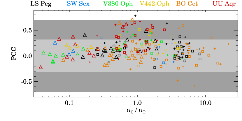
Figure 1: The Pearson correlation coefficient (PCC) as a function of the ratio of the standard deviation of the measurements of a given comparison star ($\sigma_{\mathrm{C}}$) relative to the value of the target ($\sigma_{\mathrm{T}}$). The triangles represent the photometric data, the plus signs refer to the circular polarimetry, and the squares denote linear polarimetry data. Different colours are used to distinguish each SW Sex star of our sample. We compare each target with more than one field star. This procedure results in a number of points having the same color and symbol. The points inside the light grey region do not present correlation, as explained in text. The dark grey region contains data sets that should be inspected individually to verify the presence of correlation.

The small number of targets allow us to perform an individual and careful analysis of each source to take into account its peculiarities. Therefore, some adjustments to the procedure were performed when required. The detailed analysis and results for each source are described in Section 4.

4 Results and analysis

In the following sections, we present an overview of previous findings, our results on a period search, and our analysis of the presence of magnetic accretion in each object of our sample. Table 4 presents the main periods found in the literature as well as those found in this paper.

Table 4: Claimed periods from literature and from our analysis. We indicate our periods having small confidence levels with a trailing question mark.

Object	Period	Data	Interpretation	Reference
	3.36 h	Photometry	Porb	1
	19.9 $\pm$ 0.9 min	Spectroscopy (H$\alpha$ RV)	Pspin	2
	19.6 $\pm$ 0.9 min	Spectroscopy (H$\alpha$ EW)	Pspin	2
	50.9 $\pm$ 0.5 min	Photometry	—	This work
BO Cet	19.7 min	Photometry	—	This work
	15.3 min	Photometry	—	This work
	11.1 $\pm$ 0.08 min	Circular Pol.	Pspin	This work
	9 min	Circular Pol.	Pbeat (50.9 - 11.1)	This work
	14 min	Circular Pol.	Pbeat (50.9 - 11.1)	This work
	3.24 h	Photometry	Porb	3
SW Sex	22.6 $\pm$ 1.4 min	Photometry	Pspin/2	This work
	41.2 $\pm$ 8.5 min	Circular Pol.	Pspin	This work
	2.98 h	Spectroscopy (RV)	Porb	4
	4.37 d	Photometry	PW	5
	2.90 h	Photometry	PSH-	5
	16.66 min	Photometry	QPOs	5
V442 Oph	16.0 min	Photometry	QPOs?	5
	19.5 min	Photometry	QPOs?	5
	12.4 $\pm$ 0.09 min	Photometry	—	This work
	19.4 $\pm$ 0.4 min (?)	Circular Pol.	Pspin	This work
	18.3 $\pm$ 1.1 min (?)	Linear Pol.	Pspin	This work
	3.70 h	Spectroscopy (H$\alpha$ RV)	Porb	2
	4.51 d	Photometry	PW	6
	3.56 h	Photometry	PSH-	6
	46.7 $\pm$ 0.1 min	Spectroscopy (H$\alpha$ EW)	Pspin	2
V380 Oph
	47.4 $\pm$ 4.9 min	Photometry (V band)	—	This work
	12.4 $\pm$ min	Photometry (B band)	Pspin?	This work
	22.0 $\pm$ 1.2 min (?)	Circular Pol.	Pspin?	This work
	12.7 $\pm$   min (?)	Circular Pol.	Pspin?	This work
	4.2 h	Spectroscopy (H$\alpha$ RV)	Porb	7,8
	20.7 $\pm$ 0.3 min	Photometry	QPOs	7
	19 min	Photometry	Pspin?	9
	16.5 $\pm$ 2 min	Photometry	—	10
	19 min	Photometry	QPOs	11
	$\sim$20 min	Spectroscopy	QPOs	12
	33.5 $\pm$ 2.2 min min	Spectroscopy	Pbeat	13
LS Peg	29.6 $\pm$ 1.8 min	Circular Pol.	Pspin	13
	30.9 $\pm$ 0.3 min	X-rays	Pspin	14
	21.0 $\pm$ 1.2 min	Photometry	Pbeat (Porb - Pspin)	This work
	16.8 min	Photometry	—	This work
	19.3 min	Photometry	—	This work
	24.2 min	Photometry	—	This work
	18.8 $\pm$ 0.005 min	Circular Pol.	Pspin	This work
	11.5 $\pm$ 0.1 min	Linear Pol.	Pspin/2	This work
	3.9 h	Photometry	Porb	15
	4.2 h	Photometry	PSH+	16
UU Aqr	4 d	Photometry	—	17
	54.4 $\pm$ 0.5 min	Photometry	2 Pspin	This work
	25.7 $\pm$ 0.23 min	Circular Pol.	Pspin	This work

Note. — P_orb: orbital period; P_spin: spin period; P_beat: beat period ; P_SH+: positive superhump period; P_SH-: negative superhump period; P_W: Disk wobble period

References. — (1) Bruch (2017), (2) Rodríguez-Gil et al. (2007b), (3) Groot et al. (2001), (4) Hoard et al. (2000), (5) Patterson et al. (2002), (6) Shugarov et al. (2005), (7) Taylor et al. (1999), (8) Martínez-Pais et al. (1999), (9) Garnavich & Szkody (1992), (10) Szkody et al. (1994a), (11) Szkody et al. (2001), (12) Szkody et al. (1997), (13) Rodríguez-Gil et al. (2001), (14) Baskill et al. (2005), (15) Baptista et al. (1996), (16) Patterson et al. (2005), (17) Bruch (2019)

4.1 BO Cet

BO Cet was first classified as a nova-like CV with V $\approx$ 14 – 15 mag by Downes et al. (2005). Its spectrum displays the typical single-peaked H I emission lines of SW Sex systems, along with double-peaked He I and relatively strong He II 4686 Å emission (Zwitter & Munari, 1995). BO Cet was classified as a non-eclipsing SW Sex star by Rodríguez-Gil et al. (2007a), who published a spectroscopic study of this source. The H$\alpha$ trailed spectra show an S-wave with an amplitude of $\sim$300 km s^-1, with the bluest velocity and minimum intensity both occurring at phase 0.5, as well as a high-velocity S-wave component reaching $\sim$2000 km s^-1. This high-velocity component exhibits periodic emission-line flaring at a period of 19.9 $\pm$ 0.9 min, which is interpreted as the spin period of a magnetic WD. Its orbital period is estimated as 0.13983 d by Bruch (2017) based on the Center for Backyard Astrophysics (CBA) data. The only hitherto formally published photometric time series of BO Cet is by Bruch (2017). His data sets show strong flickering, and the orbital modulation is not always discernible.

We observed BO Cet in V and R_C bands during three runs in 2010, 2016 and 2019 (see Table 1) with exposure times between 10 and 60 s. Our data do not show any significant variation in the average magnitude in the R_C band, but the V band average varied by around 1 mag (see Table 1).

Our data are not suitable to refine the orbital period, since the individual data sets span time intervals comparable to or smaller than the orbital period, and the long term data sampling introduces a huge aliasing structure in the power spectrum. Moreover, Bruch (2017) shows that an orbital modulation is not always clearly present in BO Cet photometry.

Figure 2: Time-series analysis of BO Cet. First column: (Top panel) LS periodogram of the photometric data. The second, third, and fourth panels (from top to bottom) exhibit the magnitude, the percentage of circular polazation (P_C) and the percentage of linear polarization (P) data, folded with the 50.9 min period and an arbitrary zero phase. The second column follows the same structure of the first one, but the periodogram corresponds to the circular polarimetry data, and the curves are folded with the 11.1 min period. The dashed orange lines represent the FAP levels of 1%, 0.1%, and 0.01%, calculated according to Scargle (1982). The blue lines correspond to a central-moving average considering the points inside an interval of 0.05 in phase.

The following analysis includes only data from 2010 October 6, 11, 12, and 2016 October 19 (see Table 1), which do not show significant correlation with the measurements of the field stars, as described in Sec. 3. The photometric data were pre-whitened at the orbital period before the computation of the LS periodograms. The power spectrum peaks at P = 50.9 $\pm$ 0.5 min (Fig. 2). The strong 1-day aliasing structure hinders the determination of the exact value of this periodicity. But it is most likely real since it is well above the 0.01% false-alarm probability (FAP) line and is consistently present in the individual nights (not shown here) that are spread over a 6-years range. This peak is also present in the periodogram with no pre-whitening. The magnitude phase diagram shows a clear modulation with a semi-amplitude of around 0.05 mag (Fig. 2, second panel from top to bottom). A harmonic at around 25 min is present in the periodogram. Other peaks are seen at 19.7 min and 15.3 min.

The (no pre-whitened) circular polarimetric data show a periodic signal at 11.1 $\pm$ 0.08 min, as shown in the power spectrum of Fig. 2 (see top panel of the second column). This period is not present in the field stars, which gives us some confidence that it is not an artefact. The circular polarization data folded with the 11.1 min period reveals a sinusoidal modulation having both negative and positive polarization excursions and a semi-amplitude of around 0.1% (see the solid blue line).

Linear polarization measurements do not follow a normal probability distribution and are intrinsically biased (Clarke et al., 1983). In the case of BO Cet, the bias correction applied to the linear polarization data results in many points of null polarization. Even so, we performed the LS analysis. The power spectrum shows a variety of peaks in the region of 50 min, the same region of the strong signal in the photometry periodogram. The power of those peaks is slightly higher than the level of 0.01% of FAP. The curve folded using the strongest peak, at 54.4 $\pm$ 0.9 min, does not show any coherent variation, therefore we do not show any figure related to the linear polarization data.

The main circular polarization peak at 11.1 min has adjacent structures centered at about 9 min and 14 min (Table 4), which are consistent with the positive and negative beats of the main peak with the 50.9 min photometric main period. The presence of the beat periods between the main photometric and polarimetric peaks supports the reality of these periods. The periodicity of 11.1 min found in circular polarization corroborates that BO Cet could harbour magnetic accretion, as suggested by Rodríguez-Gil et al. (2007a). In this IP scenario, the photometric signal at $\sim$51 min could be associated with a continuum radiation source located in the inner disk region. In particular, this region could be at the magnetosphere radius, where the mass flow starts to follow the magnetic field lines and leaves the orbital plane.

Rodríguez-Gil et al. (2007a) found a period of 19.9 min from the radial velocities of the H$\alpha$ line wings, consistent with a 19.6 min period from the equivalent widths of the H$\alpha$ blue wing. They suggested this to be associated with the WD rotation period. As the origin of the circular polarization is more directly connected with the WD rotation, we suggest that the WD spin period is 11.1 min. Interestingly, our photometric power spectrum also shows a peak at around 19.7 min, which could be related to the line-emission source detected by Rodríguez-Gil et al. (2007a) diluted by continuum emission.

4.2 SW Sex

SW Sex, the prototype of the class, was discovered in the Palomar-Green survey by Green et al. (1982). Follow-up spectroscopy and photometry (Penning et al., 1984) showed high-excitation emission lines, a deep eclipse of 1.9 mag, and an orbital period of 3.24 h. A refined orbital period, 0.1349384411(10) d, was obtained by Groot et al. (2001). SW Sex has been observed in two brightness states considering its magnitude out of eclipse, which has mean values of $\sim$14.2 (high state) and $\sim$15.1 (low state) in unfiltered observations calibrated with Johnson V band zeropoint, according to observations available in the American Association of Variable Star Observers website (AAVSO). Spectroscopy performed in the bright state showed the typical central absorption in the Balmer emission lines between phases 0.4 and 0.6 (e.g. Szkody & Piche, 1990). Spectrophotometric observations during the faint state of the system did not exhibit the absorption feature and emission-line flaring was not detected (Dhillon et al., 2013). No periodicity in broad band photometry is reported for this system. Circular polarimetric observations by Stockman et al. (1992) revealed no significant circular polarization in the 3200 – 8600 Å  range, with values as low as 0.05 $\pm$ 0.14% in a single 8 min integration and -0.03 $\pm$ 0.05% in 16 min. However, in a paper about the detection of circular polarization in LS Peg, Rodríguez-Gil et al. (2001) made a side note about a period of 28 min detected in the B band circular polarization of SW Sex.

SW Sex was observed by us on one single night (March 29, 2014). A time series of R_C measurements was made during 3.9 h covering one complete orbital cycle and one total eclipse. The mean magnitude out of eclipse in our photometric data is R_C= 14.66 mag, indicating that the system was in a high brightness state. The folded light curve shows a deep eclipse with amplitude of 1.6 mag, as expected (Fig. 3, first column).

The folded polarization data reveal an increase in the absolute values of circular and linear polarizations during the eclipse (Fig. 3, bottom panels). This could be interpreted as a polarized emission component that is diluted by an unpolarized light source out of eclipse. During the eclipse, part of the unpolarized component is occulted, thus reducing the dilution and making the net polarization of the system larger. Reasonable guesses as to the origin of the polarized and unpolarized components are the PSR region of a magnetic accretion column and the accretion disk, respectively. The eclipse of the PSR region could also occur. It would last less than the disk eclipse, because the PSR region is much smaller. In the polars FL Cet and MLS110213 J022733+130617, the PSR region is eclipsed during an interval of about 0.05 in the orbital cycle (O’Donoghue et al., 2006; Silva et al., 2015, respectively). In this case, the polarization should drop to zero around the middle of the eclipse, producing an “M” shaped polarization pattern. As it is not observed, we can conclude that the PSR region is not eclipsed in SW Sex.

To perform the period search, we removed the points associated with the eclipse from the dataset and then subtracted the orbital modulation using a third-order polynomial fit to the photometric data (e.g. Basri et al., 2011; Ferreira Lopes et al., 2015). The resulting power spectrum has one significant peak at 22.6 $\pm$ 1.4 min (see Fig. 3). This peak is also present, but with a lower power, if we do not subtract the orbital modulation. The light curve folded at this period displays a modulation with an amplitude of about 0.11 mag.

The period search in the polarimetric data was also performed removing the eclipse points. The periodogram of circular polarization shows a peak at 41.2 $\pm$ 8.5 min. The mean polarization in the phase diagram ranges between -0.2% and 0.2% (blue line in circular polarization panel of the last column of Fig. 3). Interestingly, the photometric period (22.6 min) is consistent with the first harmonic of the period found in polarimetry (41.2 min), considering the uncertainties in the peak position. The phase diagrams of the photometry using these two periods in Fig. 3 illustrate this. The linear polarization folded with the 41.2 min period shows a relatively well organized phase diagram. However, the highest peak in linear polarization occurs at 12.7 $\pm$ 0.7 min (below the adopted FAP levels) and the corresponding phase diagram is very noisy. Hence, we do not discuss it here. Probably, the time-series analysis of the linear polarimetry is affected by the large number of measurements consistent with zero, due to the large errorbars.

Some IPs (e.g. V405 Aur and UU Col, Piirola et al., 2008; Katajainen et al., 2010, respectively) show two maxima in the flux phase diagram, associated with positive and negative circular polarization. Our data suggest that this can also be true for SW Sex. This finding and the increase in the polarization during the eclipse support the presence of a magnetic WD rotating at around 41 min in SW Sex. Additional polarimetric observations having a longer time span would be useful to confirm these results.

Figure 3: Time-series analysis of SW Sex. First column: Phase diagrams of the photometry, circular polarimetry (P_C) and linear polarimetry (P) data, folded with the orbital period and T₀ = 2456746.704430 HJD. The eclipse phases are highlighted by the gray bar. The points in this region were not considered in the analysis presented in the following columns. Second column: the top panel shows the LS periodogram of the photometry, after subtracting the orbital modulation (see text). The panel below presents the phase diagram of the magnitude folded with P = 22.6 min and arbitrary zero phase. The third and fourth panels from top to bottom show the folded circular and linear polarization, respectively. The last column follows the same structure of the second column, but for circular polarization. The lines are colour-coded as in Figure 2.

4.3 V442 Oph

V442 Oph was identified as a CV by Szkody & Wade (1980). The typical V band brightness of V442 Oph fluctuates between around 13.2 and 14.2 mag (Szkody & Wade, 1980; Szkody & Shafter, 1983; Patterson et al., 2002). However, AAVSO data show that it can as faint as 15.5 mag. This is somewhat confirmed by Patterson et al. (2002), who affirmed that the 14 mag state corresponds to a high state. However, those authors do not mention the maximum magnitude of V442 Oph in their data. Some spectral features point to a classification as a low-inclination SW Sex star (Hoard et al., 2000): single-peaked emission lines, strong He II 4686 Å emission line, a transient absorption at 0.5 phase in the Balmer and He I lines, and a high-velocity component in H$\alpha$ at $\approx\pm$1900 km s^-1. Their spectroscopic dataset settled the orbital period as 0.12433 d (2.98 h). Long photometric campaigns show persistent modulations with periods at 4.37(15) d and 0.12090(8) d, which are interpreted as the wobble period of the disk and a negative superhump, respectively (Patterson et al., 2002). At higher frequencies, the system displays rapid flickering and periodicities around 1000 s, interpreted as QPOs. In the QPO structure of the periodogram of the best quality data, there are two distinguishable peaks at 74.0 and 89.9 cycles per day (19.5 and 16.0 min). Circular polarimetry obtained in two nights provided 0.01% $\pm$ 0.05% and -0.03% $\pm$ 0.08% with 16 min and 8 min of total integration times, respectively (Stockman et al., 1992). These values are consistent with no net circular polarization averaged over the time interval of the measurements.

We observed V442 Oph for a total of 4.06 h spread over two nights: 2014, March 29 and 2014, July 20 (Table 1). Light curves in R_C and V filters were obtained using exposure times of 20 s and 30 s, respectively. The time series has some gaps repeating on time scales of half an hour, so we limit our analysis to a maximum period of 30 min. The mean magnitudes during each day of our observations are quite similar, R_C = 13.37 mag and V = 13.60 mag. Such values indicate that we observed V442 Oph in its typical high state.

We performed a period search in R_C and V photometric time series independently and found a period of around 12 min in both cases. No pre-whitening or detrending was applied to the data. Finding the same period in two independent data sets, obtained about four months apart, suggests the presence of a stable periodicity in V442 Oph. The power spectrum of the combined photometry has a prominent peak located at 12.4 $\pm$0.09 min (see first column of Fig. 4). The data folded using this period and an arbitrary epoch at HJD 2456859.4033 show a near sinusoidal profile with a semi-amplitude around 0.04 mag (second panel). The folded circular polarimetric curve also shows a slight modulation with an amplitude of around 0.1% (blue line in the third panel). A peak at 19.9 min with 0.1% false-alarm probability merits attention, since it also appears in the circular and linear power spectra — see below.

The power spectra of the circular and linear polarization show peaks at 19.4 $\pm$ 0.4 and 18.3 $\pm$ 1.1 min, which are below the FAP lines of 0.1% (Fig. 4, middle and right columns). The data folded at these periods do not show clear modulations, but we suggest that there could be a real periodicity of the system around 19 min. Besides being present in the periodograms of flux, circular and linear polarizations - even though with a weak signal - a similar period is also found by Patterson et al. (2002, see Table 4). They commented that the modulation semi-amplitude at this frequency is around 0.01 mag and that it is not easily detectable among other variability also present in the light curves, features which are consistent with our folded curves. As this period is present in polarimetric data, its natural explanation is the WD rotation.

In spite of the low signal, we suggest that the 19.4 min modulation found in V442 Oph is due to the WD rotation. However, we have no explanation for the 12 min modulation seen in the total flux. In particular, we could not explain this modulation as a beat between other periodicities of the system.

Figure 4: Time-series analysis of V442 Oph. First column, top to bottom: the LS periodogram from photometry; the phase diagram of the magnitude folded with 12.4 min and an arbitrary zero phase; the same as above for the circular polarization; and the phase diagram of the linear polarization using the same period. The second and third columns follow the same structure of the first column, but the periodograms are done using the circular and linear polarization data, respectively. The orange and blue lines follow the definition of previous figures.

4.4 V380 Oph

V380 Oph was reported as a nova-like CV with orbital period of 3.8 h based on spectroscopic observations (Shafter, 1985). Using archival data and new photometric observations, Shugarov et al. (2005) showed that V380 Oph is usually at 14.5 mag, but underwent a faint state (around 17 mag) in 1979. Hence, they suggested that the system can be classified as a VY Scl object. Indeed, the VY Scl behaviour of V380 Oph is confirmed by additional data presented by Shugarov et al. (2016) and the light curves available at AAVSO. Shugarov et al. (2005) also found two photometric periods, 3.56 h and 4.51 d, interpreted as due to negative superhumps and an eccentric wobbling accretion disk, respectively. Time-resolved spectra obtained by Rodríguez-Gil et al. (2007a) show the standard characteristics of the SW Sex class, single-peaked emission lines and a high-velocity S-wave in the H$\alpha$ trailed spectra. Their radial-velocity curve provided an orbital period of 3.69857(2) h, consistent with the period obtained by Shafter (1985). They also suggest the presence of rapid flaring in the line wings with a periodicity of 46.7 $\pm$ 0.1 min, which they proposed as the rotation of a magnetic WD. Optical photometry of V380 Oph performed by Bruch (2017) is consistent with an orbital modulation and reveals a flickering activity that is compatible with VY Scl systems. White-light circular polarimetry was performed by Stockman et al. (1992), who obtained a signal consistent with zero, P_C = -0.12 $\pm$ 0.16%, in a short 8 minute integration.

Figure 5: Time-series analysis of V380 Oph. First column: B band photometric data from SOS/SAS observatories. Second column: V band photometric data from OPD observatory. Third column: V band circular polarimetric data from OPD observatory. From top to bottom: the power spectrum; the phase diagrams of B band and V band photometry, and circular and linear polarizations. The coloured lines are as defined in Figure 2.

V380 Oph is the only object of our sample for which we have additional data obtained from observatories other than OPD (see Section 2 and Table 1). We reanalyzed the SOS/SAS V380 Oph photometric data (Shugarov et al., 2016) obtained from 2002 to 2016 searching for short periods possibly associated with the WD rotation. Typically, V380 Oph has a mean magnitude of approximately 15 mag (high state). During three nights on 2015 July 15 to 22, a low state was detected in the R_C band with an average brightness of 18.8 mag.

Initially, we present the periodicity analysis of the time series obtained at SOS/SAS observatories. The V band data were obtained over many years and are characterized by data blocks with time spans from around 1 to 4 h. The LS power spectrum (not shown here) is very complex. It shows a clear signal at around 4.5 d, as previously reported. The peak is broad and highly structured. A stronger and narrower peak at around 1.3 d is also present. We have filtered the time series using the main peaks relative to periods on a timescale of days. The periodograms remain very complex with many peaks on timescales of hours and days. No clear signal on a minutes timescale could be found. We also studied the data sets on a daily basis and no clear signal appears. We applied the clean technique (Roberts et al., 1987) in order to verify if we could obtain a better understanding of the photometric variability, but the results are essentially the same as those obtained using the LS method. The R_C data in the bright state are sparser and have shorter daily data blocks compared to the V band. The results are essentially the same for both bands. The R_C data set in the low state is composed of 3 daily blocks: no clear periodicity is found. The $B$ band periodogram has a very broad feature at around 55 min, which is badly constrained by the short time span of about 2 h. Similar features are present in some power spectra of V and R_C daily data blocks. A peak at 12.4 min is present below a FAP of 1%. Fig. 5 (left column) shows the power spectrum and the data folded on 12.4 min. There seems to be a coherent modulation of the circular polarization at this period. After removing the orbital modulation, only the 12 min peak remains, yet below the 1% FAP.

Our OPD observations were performed in the V band on a single night, 2014 July 19, having a total time span of $\sim$2.7 h with 40 s of exposure time. The system was in the usual high state at around 14.5 mag. The power spectrum of the photometry shows a periodicity at 47.4 $\pm$ 4.9 min (Fig. 5, middle column). This period is in the upper limit of the range of reliable periods due to the total time span of the observation. However, it is consistent with the $\sim$47 min flaring period reported by Rodríguez-Gil et al. (2007a).

The circular polarimetry periodogram shows a peak at 22.0 $\pm$ 1.2 min with a level similar to the 0.1% FAP (Fig. 5, right column). After removing the orbital modulation, we obtained a period at 12.7 $\pm$ 0.4 min above the 0.01% FAP (not shown), which is similar to that found in the B band data obtained at the SOS/SAS observatories. In this case, the modulation in circular polarization is similar to that shown in Fig. 5, left column, therefore we do not present a figure with exactly this period. In the linear polarimetry data, we found 17.7 $\pm$ 1.5 min. However, the same period is also found in one field star, consequently this period can be related to instrumental effects and is suspicious.

In addition to its complex photometric behaviour, V380 Oph also shows variation in the measured values of the radial velocity amplitude depending on its brightness state (see Szkody et al., 2018, and references therein), which could be related to the variation of the accretion-disk size. Zellem et al. (2009) obtained the UV spectrum of V380 Oph, which is too red to be fitted with an optically-thick accretion-disk model. A possible interpretation is an accretion disk truncated in its inner parts in an IP-like configuration. These facts together with the presence of line flaring (Table 4) and a possible periodicity in circular polarimetry may indicate magnetic accretion. But, we consider additional polarimetric and spectroscopic observations are important to corroborate these findings.

4.5 LS Peg

LS Peg was classified as a CV by Downes & Keyes (1988). It has high and low states ranging from V = 12 to 14 mag (Garnavich & Szkody, 1992). UV spectra at the high state led Szkody et al. (1997) to propose LS Peg as a non-eclipsing SW Sex object. Taylor et al. (1999) estimate an orbital period of 0.174774(3) d based on radial velocity curves. The first detection of modulated circular polarization in an SW Sex system was obtained for LS Peg: the circular polarization values were the result of the integration in the 3900 – 5070 Å range of spectropolarimetric data and are consistent with a periodicity of 29.6 $\pm$ 1.8 min and amplitude of $\sim 0.3\%$ (Rodríguez-Gil et al., 2001). Those authors suggested that this modulation corresponds to the WD spin. That paper also shows the presence of flaring in the H$\beta$ emission line with a period of 33.5 $\pm$ 2.2 min, which the authors interpreted as the beat period between the WD spin period (29.6 min) and the orbital period. Baskill & Wheatley (2006) reported a detection of a period at 30.9 $\pm$ 0.3 min in X-ray data obtained by ASCA SISO (2 – 8 keV). However, this modulation was not confirmed by the XMM-Newton observations of LS Peg in the 0.1 – 12 keV energy range (Ramsay et al., 2008). These authors mentioned that the X-ray spectrum of LS Peg is similar to those of IPs.

Our data on LS Peg were obtained on 7 nights between 2010 and 2019 in V and R_C bands (Table 1). The photometric light curves show a mean magnitude of 11.9 mag and 11.7 mag in V and R_C bands, respectively. Data from two nights were removed from the periodicity analysis (see Sect. 3) that was performed combining the data in three ways: all observed bands, combining data by filters, and the individual nights.

The mean magnitude was subtracted from the photometric data set of each night, which were also filtered to remove low-frequency modulations. The resulting power spectrum exhibits the strongest peak at 21.0 $\pm$ 1.2 min (see top of the first column of Fig. 6). This period is consistent night-by-night, except for two of them (see Table 5). However, these nights do have a secondary peak around 20 min. The light curve folded on the 21 min periodicity shows a sinusoidal modulation with a semi-amplitude of 0.02 mag. Circular and linear polarization combining the two bands folded on the same period do not show a coherent variability (see first column of Fig. 6). The other “high-frequency” peaks seen in the power spectra are 16.8 and 24.2 min. A peak at 19.3 min superimposed on the main peak is also present. Taylor et al. (1999) found a photometric period of 20.7 min in a photometric time series collected on 12 nights spread over 18 days. The modulation was not stable in phase. Modulations around 19 min and 16 min have already been reported by Garnavich & Szkody (1992) and Szkody et al. (2001).

Table 5: Periods found in LS Peg data set.

Data	Date Obs.	Period
		(min)
	All nights	21.0 $\pm$ 1.2
	2010 Oct 06	21.4 $\pm$ 4.0
Photometry	2010 Oct 12	19.7 $\pm$ 1.7
	2016 Oct 19	40.3 $\pm$ 6.7
	2019 Sep 10	23.3 $\pm$ 3.7
	2019 Sep 12	13.9 $\pm$ 1.4
	All nights	18.8 $\pm$ 0.005
	2010 Oct 06	19.0 $\pm$ 1.6
Circular polarimetry	2010 Oct 12	18.6 $\pm$ 1.2
	2016 Oct 19	44.4 $\pm$ 5.8
	2019 Sep 10	18.4 $\pm$ 3.4
	2019 Sep 12	17.8 $\pm$ 2.1

Circular polarization data were not prewhitened. The periodogram of the entire data set shows a sharp peak centred at 18.8 $\pm$ 0.005 min (see top of the second column of Fig. 6). This same period is also seen if we combine all 2010 data or all 2019 data. This suggests that LS Peg has a stable periodicity in circular polarization along a baseline of 9 years. As in photometry, the main peak in the periodogram of 2016 October 19 occurs at around 40 min (see Table 5). The circular polarization curves folded on 18.8 min exhibit positive and negative excursions with semi-amplitudes of 0.05% (blue line in third panel of second column of Fig. 6). The photometry and linear polarization do not show clear modulations at this period (see last panel).

The periodograms of the linear polarization data show strong signals at low frequencies. Hence, we prewhitened the data and found a peak at 11.5 $\pm$ 0.1 min, which could be related to half of the photometric 21 min period. A possible origin of this modulation could be the reflection (scattering) of the PSR region emission in the inner regions of the disk.

As stated above, Rodríguez-Gil et al. (2001) also detected modulated circular polarization. They found a period of 29.6 min using 19 circular polarimetry spectra with a time resolution of about 10 minutes, which results in a Nyquist frequency of around 20 min. Therefore, their data were not adequate to search for periodicities of the order of those previously found in photometry.

The periodic signals found in LS Peg (Table 4) can be interpreted in terms of WD spin, QPOs, orbital period, or the combination of those as beat periods. Since the best explanation for the presence of circular polarization is cyclotron emission from a PSR region on the WD surface, the circular polarization modulation must be attributed to the rotation of a magnetic WD. Hence, our results indicate that the period of $\sim$19 min is the spin period of the WD, consistent with previous suggestions (e.g. Szkody et al., 2018). In such a scenario, the photometric 21 min can be, within the uncertainties, the beat period between the WD spin period and the orbital period. This interpretation is in line with the linear polarization modulation at around 11 min being caused by internal scattering, since beat periodicities are usually associated with reflection of internal sources on the accretion structures.

V795 Her has spectroscopic properties very similar to LS Peg (Taylor et al., 1999; Martínez-Pais et al., 1999), indicating a similar mass accretion configuration. This object has non-null circular polarization modulated at a period of 19.54 min (Rodríguez-Gil et al., 2002), close to the periodicity attributed to QPOs in LS Peg. So, in a comparative way, this reinforces the presence of a magnetic WD in LS Peg.

Figure 6: The first column shows, from top to bottom, the power spectrum of the photometric data in V and R_C bands and the phase diagrams of photometry, circular and linear polarimetric data, folded on the period P = 21 min and arbitrary zero phase. The second column has the same structure of the first one, but the power spectrum is calculated for the circular polarization and has a peak at 18.8 min. The lines are colour-coded as in Figure 2.

4.6 UU Aqr

The variability of UU Aqr was discovered by Beljawsky (1926). More than half a century later, Berger & Fringant (1984) found that the object has a strong UV excess. Photometric monitoring performed by Volkov et al. (1986) and Volkov & Volkova (2003) confirmed the UV excess and revealed that UU Aqr has deep eclipses up to 2 mag and strong flickering outside the eclipse, establishing UU Aqr as a CV. Using multiwavelength eclipse mapping, Baptista et al. (1996) suggested that UU Aqr is an SW Sex object. This was confirmed by Hoard et al. (1998) based on spectroscopic features, even though the He II 4686 Å emission line is weak in comparison with H$\beta$ and the line absorption is deepest at orbital phase $\sim$0.8. UU Aqr has an average magnitude outside the eclipse of 13.5 mag with an eclipse depth around 1.4 mag (see Fig. 1 in Baptista & Bortoletto, 2008). In the high state, a bright spot on the outer edge of the disk changes the shape of the eclipse profile. Its orbital period is 0.163580487(2) d (Borges B. & Baptista R., private communication). Using data collected in 2000, Patterson et al. (2005) found a period of 4.2 h that is attributed to the superhump phenomenon. However, Bruch (2019) did not detect superhumps in data obtained in 2018 September, only regular variations with a period of about 4 days.

UU Aqr was observed during five nights distributed between August and October 2009 (see Table 1). The V filter was used in all observations and the exposure times range between 4 s and 15 s. The magnitude was stable during those nights with an average value of V $\approx$ 13 mag. The magnitude dispersion in our data is around 0.1 mag for most nights. We found a large correlation between the photometry and polarimetry of UU Aqr and those of the field stars on some nights, so they were not considered in the analysis (see Table 1). We also removed the observations obtained during the eclipses.

The power spectrum of photometric data applying no filtering shows a strong peak at 54.4 $\pm$ 0.5 min (Fig. 7). The peak is also present if we subtract the orbital modulation from the data. The folded light curve displays a clear modulation with a semi-amplitude of around 0.2 mag. The large dispersion around the average is due to the orbital flux modulation.

We did not subtract the low frequencies from the circular polarimetric data. The periodogram shows the strongest peak at 25.7 $\pm$ 0.23 min (see second column of Fig. 7). This peak is also present in the periodograms of the individual nights, supporting the persistent nature of this periodicity. The phase diagram of the circular polarimetry shows a modulation with peak-to-peak amplitude of 0.1% (blue line). We did not find any statistically significant periods in the linear polarimetry.

As already discussed for the other objects, the only possible explanation for a periodic variability in circular polarization is the presence of a PSR region near the WD surface. Hence, the 26 min could be associated with the spin period of a magnetic WD. An argument in favour of this is the presence of a modulation with nearly twice this period in the photometry (Table 4). Another indirect evidence of a magnetic WD in UU Aqr comes from the observation of variability on timescales of 0.5 – 5 days during stunted outbursts (Robertson et al., 2018) who suggested it to be caused by “blobby” accretion associated with the fragmentation of the stream by the magnetic field.

In order to confirm the stability of the 26 min period and consequently the magnetic nature of the WD in UU Aqr, it is necessary to obtain additional polarimetric data. It is important to mention that the strong flickering of UU Aqr makes difficult to search for real periodic variabilities. The flickering is not polarized but, being a variable emission that dilutes the polarization, it can introduce noise in the polarization signal. It can also produce fake peaks in the total flux periodogram.

Figure 7: Time-series analysis of UU Aqr. From top to bottom, the power spectrum of the photometry and the phase diagrams of photometry, circular and linear polarization. The first column shows the photometric results and the second column presents the period search in circular polarization data. The coloured lines are as defined in Figure 2.

5 Discussion

5.1 Present status of circular polarization measurements of SW Sex systems

We have performed polarimetry of 6 definite SW Sex systems. In four of them (BO Cet, SW Sex, LS Peg, and UU Aqr), we have found evidence of modulated circular polarization. For V442 Oph and V380 Oph, the detection of circular polarization is uncertain.

Table 8 summarises all circular polarization measurements of SW Sex systems. This table is strongly based on information presented in The Big List of SW Sex Systems of Hoard et al. (2003). We included the results of this paper and made some other changes, as follows. RR Pic is quoted as polarized in The Big List, but this measurement refers to linear polarization, which could originate from other mechanisms than emission from the PSR region. Therefore, it is not evidence of magnetic accretion and, hence, it is not included in Table 8. We have also changed the “polarized” classification of AO Psc from “N?” to “Y?”, since it has some evidence of modulation in circular polarization, but the errors are not small enough to confirm it. This object is also classified as an IP (e.g. Butters et al., 2009). As a result, our table lists 27 systems, including BO Cet and UU Aqr for which the first measurements are presented here. The first lines of the table group the objects having confirmed or possible non-null circular polarization.

A large fraction of the polarimetric observations of SW Sex systems was performed by Stockman et al. (1992). Their observations consist of a single or a few measurements. Each measurement is the result of data taken over an interval of 8 min (or even longer), which is inadequate to detect the circular polarization in these objects because the timescale of the modulation is usually of this same order, causing the smearing of an intrinsically low polarization signal. Hence, their negative detections are unreliable. Some other measurements in Table 8 classified as “polarized = N?” refer to long integrations with the same caveat of Stockman et al. (1992)’s measurements. High signal-to-noise and time-resolution of around 1 min are necessary to detect circular polarization in SW Sex systems.

According to The Big List, there are 73 objects classified as SW Sex. They are divided into 30 definite, 18 probable, and 25 possible candidates. Table 8 lists 11 objects with some evidence of non-null circular polarization: this results in 15% of SW Sex systems with evidence of magnetic accretion from polarimetry. This is a non-negligible fraction since few objects have been observed with enough sensitivity and time resolution. If we consider only the definite SW Sex members, we obtain 33% (10/30) of possible polarized objects. Taking into account only objects with confirmed modulated circular polarization, this fraction decreases to 23% (7/30).

The above numbers may reveal the presence of magnetic WDs in a considerable fraction of SW Sex stars. More polarimetric observations like the ones presented in this paper are in demand to confirm previous measurements and expand the sample of observed SW Sex objects.

5.2 Periodicities in asynchronous magnetic CVs

In this section, we discuss the main findings related to rapid variability in SW Sex and compare them with what is observed in IPs.

SW Sex systems usually show complex photometric variability. In some systems, periodicities related to the WD rotation, orbital cycle, or sidebands have been found, similar to what is observed in some IP systems (e.g. Warner, 1986; Norton et al., 1996). Superhumps, with periods slightly longer or shorter than the orbital period, are also present in some systems and are attributed to the precession of an eccentric accretion disk or disk warping. Another photometric variability common in the SW Sex class is quasi-periodic oscillations with time scales of 1000 s. Patterson et al. (2002) present a review of these different kinds of variability and propose that some of them can be explained by a magnetic WD.

Non-orbital emission line periodicities are found in IPs as well as in SW Sex stars. They can be observed as modulation of the total emission line flux or as “flares” in the line wings. In IPs, they are associated with the WD spin or the beat of WD spin and orbital period. Examples of detailed studies of spin-phase resolved spectroscopy of IPs are Marsh & Duck (1996, FO Aqr) and Bloemen et al. (2010, DQ Her). Doppler tomography phased on the spin cycle of seven IPs is presented by Hellier (1999). V1025 Cen is an example of the complex variability behaviour in IPs (Buckley et al., 1998), for which the interpretation of the observed periods and the relation between values found in photometry and spectroscopy are not straightforward. Rapid spectroscopic variability has been found in 8 definite and 2 possible SW Sex systems: EX Hya (Kaitchuck et al., 1987), which is classified as a possible SW Sex system by Hoard et al. (2003); LS Cam (Dobrzycka et al., 1998); BT Mon (Smith et al., 1998); LS Peg (Rodríguez-Gil et al., 2001); V533 Her (Rodríguez-Gil & Martínez-Pais, 2002); BO Cet and V380 Oph (Rodríguez-Gil et al., 2007a); V1084 Her (Rodríguez-Gil et al., 2009); DW UMa (Dhillon et al., 2013); and SDSS J075653.11+085831.8, in which the flaring is visible but no periodicity was found (Tovmassian et al., 2014). The periods range from 16 to 50 min. Some authors suggested that these periods could be associated with the WD spin rotation, as in IPs.

The literature has several examples of modulated circular polarization in IPs (e.g. Piirola et al. 2008 - V405 Aur - and Katajainen et al. 2010 - UU Col). The periods are the spin period or half this value. The last case is in fact explained by two maxima per cycle, hence the modulation of the polarization in IPs is always on the WD rotation. PQ Gem, for instance, presents both behaviours , depending on the band (Potter et al., 1997). Moreover, the total flux and the polarization do not necessarily vary in the same way. NY Lup and IGR J15094$-$6649 have their polarization modulated with the spin period. However, the photometry of NY Lup shows sideband periods in some bands, while the flux of IGR J15094$-$6649 modulates with the WD spin (Potter et al., 2012).

The SW Sex systems with periodic modulation in flaring and circular polarization are V1084 Her, LS Peg, BO Cet, and V380 Oph (the last two considering circular polarization from this work). Rodríguez-Gil et al. (2009) detected a period of 19.4 $\pm$ 0.4 min in the polarization of V1084 Her (RX J1643.7+3402) and twice this period in the radial velocity and equivalent width of Balmer and He II 4686 Å emission lines. The authors discussed that these observations can be understood in two ways: (1) $\sim$19 min is half of the beat between spin and orbital periods and $\sim$39 min is the beat period itself or (2) $\sim$19 min is half the spin period and $\sim$39 min is the spin period. Patterson et al. (2002) obtained long photometric time series on more than 50 nights. The power spectrum shows a QPO broad bump with a superimposed narrow peak at 17.38 min, which is consistent with the beat of 19 min and the orbital period. X-ray observations show a clear orbital modulation and a possible periodicity of around 26 min (Worpel et al., 2020), at odds with any previously reported period in this range.

LS Peg is one of the objects included in this work. The periods already claimed in the literature for this object as well as those found in this work are presented in Table 4. We could not confirm the previous claim of circular polarization modulated at 29.6 $\pm$ 1.8 min (Rodríguez-Gil et al., 2001). Instead, we detected a modulation with a period of 18.8 $\pm$ 0.005 min, which is consistent with the periods systematically found in photometry (see Table 4). We also found photometric periods in the interval between 16.8 and 24.2 min. The main photometric period in our data is 21.0 $\pm$ 1.2 min, consistent with the 20.7 $\pm$ 0.3 min from Taylor et al. (1999), and also consistent with the beat between our polarimetric period and the orbital period. For V1084 Her, the photometric period is also consistent with the beat of the polarization and orbital periods, but it is larger than the polarimetric period, inversely to what is observed in LS Peg. The spectroscopic period of 33.5 $\pm$ 2.2 min (Rodríguez-Gil et al., 2001) is around twice the polarimetric period, analogous to V1084 Cen.

The results for V1084 Her and LS Peg suggest a possible relation between the periods of flaring and circular polarization, with the latter half the value of the former. BO Cet follows the same trend: a spectroscopic period of approximately 20 min (Rodríguez-Gil et al., 2007b) and a circular polarization period of 11.1 $\pm$ 0.08 min. For V380 Oph, a similar situation happens. We raised two questionable periods of 22 and 12 min. Considering the first one, the same relation between circular polarization and spectroscopic flaring (46.7 $\pm$ 0.1 min, Rodríguez-Gil et al., 2007a) would be present. In both cases, the period found for spectroscopic flaring is also present in our photometric data, i.e they have photometric periods twice the polarimetric period. The same approximate relation is seen for UU Aqr, for which no flaring was reported in the literature.

On the other hand, SW Sex and V442 Oph have polarimetric periods (uncertain for V442 Oph) approximately twice the photometric periods. Rapid spectroscopic variability was not reported for these two objects.

Magnetic WDs in spin-rate equilibrium can have different types of accretion flow depending on the ratio between the WD rotation period, P_spin, and the orbital period, P_orb (Norton et al., 2008). Considering a mass ratio of 0.5, the conditions for the different accretion geometries are the following: P_spin/P_orb $\lesssim$ 0.1 will be disk-like; 0.1 $\lesssim$ P_spin/P_orb $\lesssim$ 0.6 will be stream-like, and P_spin/P_orb $\sim$ 0.6 will be ring-like. In all cases, the material is propelled in order to maintain angular momentum balance. The magnetic scenario for SW Sex stars proposed by Rodríguez-Gil et al. (2001) has a magnetosphere radius extending up to the corotation radius with a corresponding relation between P_spin and P_orb given by:

$$P_{\rm spin}\approx 0.31f^{3/2}P_{\rm orb},$$ (1)

where $f$ is the corotation radius in units of R${}_{L_{1}}$, which is the distance between the inner Lagrangian point L₁ and the WD.

Table 6 shows the results of the relation P_spin/P_orb and $f$ for our sample of objects, considering the periodicities found in this paper and interpreted as the P_spin. BO Cet, V442 Oph, V380 Oph, LS Peg and UU Aqr can be classified as disk-like and their $f$ values are consistent with the interval of 0.4 – 0.6 R${}_{L_{1}}$ (Groot et al., 2001). Only SW Sex itself exhibits the accretion flow as stream-like, and a corotation radius of 0.7 R${}_{L_{1}}$, slightly larger than the value measured by Groot et al. (2001).

Table 6: Relations of orbital period and spin period considering our results.

Object	Porb	Pspin	Pspin/Porb	$f$
	(min)	(min)		(R${}_{L_{1}}$)
BO Cet	201.36	11.1	0.06	0.32
SW Sex	194.31	41.2	0.21	0.78
V442 Oph	179.07	19.4	0.11	0.50
V380 Oph	221.91	12.7	0.06	0.32
LS Peg	251.67	18.8	0.07	0.39
UU Aqr	235.56	25.7	0.11	0.50

5.3 Inclination versus polarization

The SW Sex class was initially supposed to be composed only of eclipsing systems. In spite of the discovery of an increasing number of non-eclipsing systems, more than a half of the SW Sex systems are eclipsing, which is not consistent with a homogeneous distribution of inclinations. For the present discussion, it is not relevant if this is an observational or historical bias or a physical characteristic of the SW Sex phenomenon.

Notwithstanding the small number of objects, Table 8 shows that 73% (8/11) of SW Sex stars with possible circular polarization are non-eclipsing systems. If we focus only on objects with confirmed circular polarization, 4 out of 7 are non-eclipsing. Therefore, there is a higher incidence of polarized objects among non-eclipsing systems.

A possible origin for such a correlation could be the following. In the magnetic accretion scenario, the cyclotron emission is produced very near the WD surface . The accretion disks of SW Sex systems could block the direct view of the PSR region in high-inclination systems, which would prevent us from observing the polarized component in the total system emission at all phases. On the other hand, the flux from the disk increases with its projected area, which makes the dilution of a possible PSR region emission larger for lower inclinations. Hence, there should be an optimal inclination where the detection of the polarization would be most favoured. This inclination is likely near the maximum inclination for which no eclipse is seen.

5.4 SW Sex stars in X-rays

In addition to the optical cyclotron emission, the material in the postshock region also cools by bremsstrahlung emission in X-rays. Hence, models of the optical and X-ray emission of magnetic CVs can be used to constrain their physical and geometrical properties (e.g. Silva et al., 2013; Oliveira et al., 2019). The flux is usually modulated with the WD rotation due to variable absorption with the viewing angle or occultation of the emitting region by the WD. Mukai (2017) presents a comprehensive review on X-ray emission from accreting WDs. In this section, we briefly overview the X-ray emission of SW Sex objects.

Table 7 shows the SW Sex objects that have X-ray counterparts. They add up to 10 objects, corresponding to $\sim$14% of the 73 systems of The Big List. Five of them have reported periodicity and two of them are also classified as IPs: EX Hya (Hellier et al., 2000) and AO Psc (Hellier & van Zyl, 2005).

Three SW Sex systems are X-ray sources and have positive polarization : LS Peg, V533 Her, and V1084 Her. Ramsay et al. (2008) did not find any periodicity in further X-ray data (see also Section 4.5). V533 Her and V1084 Her have been recently studied by Worpel et al. (2020) using XMM-Newton. V533 Her has low X-ray luminosity and its light curve exhibits an uncertain periodicity of 22.48 min, which is close to (but inconsistent with) the 23.33 min periodicity detected in the equivalent width of emission lines by Rodríguez-Gil & Martínez-Pais (2002). The relation between these two periods cannot be explained by a beat with the orbital period. Worpel et al. (2020) reported an X-ray periodicity of around 26 min for V1084 Her, which does not correspond to the optical circular polarization period or any other periodicity reported from optical photometry or spectroscopy.

From the above discussion, there is no evidence of magnetic accretion from the X-ray light curves of SW Sex systems. Patterson et al. (2002) discussed if the absence/small levels of X-ray emission is inconsistent with the magnetic scenario. They proposed that the high density in the accretion column could prevent the shock, which hinders the gas to reach keV temperatures. However, the subject is far from being settled. Hopefully, forthcoming X-ray surveys (e.g. e-Rosita) will shed light on this topic.

Table 7: SW Sex stars detected in X-rays. A question mark indicates uncertainty in the period.

Object	P	Reference
	(min)
LS Peg	30.9 $\pm$ 0.3	Baskill & Wheatley (2006)
LS Peg	–	Ramsay et al. (2008)
V533 Her	22.48 (?)	Worpel et al. (2020)
V1084 Her	25.82 (?)	Worpel et al. (2020)
AO Psc	13.4 (Pspin)	Johnson et al. (2006)
AH Men	–	White et al. (2000)
EX Hya	67 (Pspin)	Heise et al. (1987)
DW UMa	–	Hoard et al. (2010)
WX Ari	–	White et al. (2000)
PX And	–	White et al. (2000)
UX UMa	–	Pratt et al. (2004)

5.5 CV demography and SW Sex systems

Schwope (2018) and Pala et al. (2020) have provided volume-limited studies of CVs, considering distances from the Gaia second data release. The latter provide 42 systems within 150 pc. This sample is dominated by systems with low mass-transfer rate: it contains only three nova-like CVs including one SW Sex object (EX Hya, which is compiled in that work as an IP). They found that 36% of the objects host a magnetic WD. The sample is dominated by objects below the period gap (83%), but the fractions of magnetic systems below and above the gap are around the same, 37% and 28% respectively, considering the small number of objects. If the fraction of magnetic CVs does not depend on the mass-transfer rate or the orbital period, we would expect that around 36% of the nova-like CVs would harbor a magnetic WD. Here, nova-like variables stand for high mass-transfer rate CVs that are not polars or IPs. The fraction of SW Sex systems among the nova-like systems in the Ritter & Kolb (2003) catalog (version 7.24) is 46%, which is numerically consistent with the assumption that SW Sex systems are the missing magnetic nova-like CVs.

5.6 SW Sex stars in the context of the evolution of cataclysmic variables

The CVs in the orbital period range between 3 and 4 hours that have sufficient observations show at least some SW Sex characteristics. A possible interpretation is that all long-period CVs have to evolve through this SW Sex regime before entering the period gap (e.g. Rodríguez-Gil et al., 2007b; Schmidtobreick et al., 2012). In fact, the number of dwarf novae around 4 h decreases in comparison with the number of SW Sex stars. In this scenario, the SW Sex stars represent an important stage in CV evolution.

CVs evolve towards shorter orbital periods driven by angular momentum loss through magnetic braking and gravitational radiation (e.g. Paczyński, 1967; Verbunt & Zwaan, 1981). In addition to these mechanisms, there is additional angular momentum losses due to mass transfer itself, usually called consequential angular momentum loss (CAML, e.g. King & Kolb, 1995). Reasonable candidates for this sort of angular momentum loss include nova eruptions and circumbinary disks, among others. In the last couple of years, evidence supporting the importance of CAML in CV evolution has been growing (e.g. Schreiber et al., 2016; Nelemans et al., 2016; Liu & Li, 2016), especially regarding stability for dynamical mass transfer and the required extra angular momentum loss below the orbital period gap (Knigge et al., 2011; Pala et al., 2017). In particular, the empirical formulation by Schreiber et al. (2016) provides an explanation for the paucity of helium-core WDs among the CV population (Zorotovic et al., 2011; McAllister et al., 2019), as well as the space density and the fractions of short- and long-period systems consistent with observations (Belloni et al., 2020; Pala et al., 2020). In addition, it can also explain the properties of detached CVs crossing the orbital period gap (Zorotovic et al., 2016), the existence of single helium-core WDs (Zorotovic & Schreiber, 2017), and the mass density of CVs in globular clusters (Belloni et al., 2019).

CAML might solve several problems of the CV evolution model, but not all of them. There are some inconsistencies between predictions and observations that are most likely connected to our ignorance of magnetic braking. One prescription widely used in CV investigations is that proposed by Rappaport, Verbunt, & Joss (1983).

A well-known problem of this prescription, which is directly related to this work, is the contradiction between the expected mass-transfer rates among SW Sex stars (given the brightness of such systems) and the predicted ones (e.g. Rodríguez-Gil et al., 2007b). Indeed, SW Sex stars cluster at the upper edge of the orbital period gap, between $\sim 3$ and $\sim 4$ h. According to the prescription by Rappaport, Verbunt, & Joss (1983), the mass-transfer rate drops as a CV ages, which means that just above the orbital period gap, this prescription provides the lowest mass-transfer rates. On the other hand, the mass-transfer rates expected from the characteristics of SW Sex stars are supposed to be the highest among all CVs.

Other evidence that the magnetic braking prescription should be different were recently provided by Belloni et al. (2020) and Pala et al. (2020), who showed that the observed and predicted fractions of period-bouncers are in serious disagreement, with those predicted being much larger than observed. In addition, these authors showed that the evolutionary trend in the WD effective temperature above the period gap, which is directly connected with the mean mass-transfer rate, is opposite to the observed one. Finally, Fuentes-Morales et al. (2020) showed that the predicted fraction of old novae just above the orbital period gap is much smaller than the observed fraction. These four pieces of evidence point towards a needed revision of the magnetic braking prescription. SW Sex stars are therefore important objects in this context, which can provide significant constraints on the CV evolution model, especially considering that they are more abundant than period bouncers and long-period CVs having WDs with measured effective temperatures.

We note, however, that there is some progress in this regard. Knigge et al. (2011) provide a list of magnetic braking recipes, which are illustrated in their Fig. 2. Among them, the formulation developed by Kawaler (1988) clearly predicts an increase in the angular momentum loss rate when the CV evolves towards shorter orbital periods, which would, in turn, provide the largest mass-transfer rates just at the upper edge of the orbital period gap. This could potentially explain the expected mass-transfer rates of SW Sex stars, which could make SW Sex stars a natural stage in the long-period CV pathway. Additionally, the observed distribution of WD effective temperatures versus orbital period could be reproduced. Belloni et al. (in preparation) upgrade the prescription by Kawaler (1988) and show these and other issues related to magnetic braking might be solved.

5.7 Origin of magnetic cataclysmic variables

There are currently two main scenarios that could account for the formation of magnetic WDs in close binaries. In the first one, during common-envelope evolution, a dynamo driven by shear due to differential rotation in the hot outer layers of the degenerate core (Wickramasinghe et al., 2014) would be responsible for the magnetic field generation. This idea was originally designed for single WDs, but was generalized by Briggs et al. (2018), who extended the model to the case in which the binary survives the common-envelope evolution. However, Belloni & Schreiber (2020) detected several flaws in this model. One of them is the difficulty in explaining the complete absence of hot and young WDs among the population of post-common-envelope WD $+$ late-type main-sequence stars (e.g. Parsons et al., 2021, and references therein). In addition, the predicted fractions of magnetic WDs in the different populations of close binaries are much higher than the observed ones.

An alternative scenario for the origin of single low-field magnetic WDs was proposed by Isern et al. (2017), who argued that a dynamo similar to those operating in planets could be responsible for weak magnetic field generation in WDs. This is possible because, once the WD temperature becomes low enough, its interior starts to crystallize, which, in turn, allows the generation of a magnetic field through a dynamo. This scenario, if applied to close binaries, could help to explain the low-temperature WDs in the population of detached magnetic post-common-envelope binaries. However, the magnetic fields predicted by Isern et al. (2017) are much weaker than those observed in magnetic WDs among the different population of close binaries.

If all or part of SW Sex systems have high-magnetic moment (e.g. Patterson et al., 2002), any theory aiming to explain the origin of high-field magnetic WDs would need to account for their properties. That said, SW Sex stars are important pieces to constrain evolutionary models of CVs, and understanding whether they are predominantly magnetic or not, should provide useful constraints to any model aiming to explain the origin and evolution of magnetic WDs in close binaries.

6 Conclusions

We reported time-series analyses of photometric and polarimetric data of six SW Sex stars. We associated the periodicities found in circular polarization with the spin period of a magnetic WD, based on the assumption that the polarized flux is related to cyclotron emission from a PSR region. We found the following periods from polarimetry: 11.1 min in BO Cet, 41.2 min in SW Sex, and 25.7 min in UU Aqr. We also found uncertain periodicities (below the FAP level of 1%) of 22.0 min and 19.4 min for V380 Oph and V442 Oph, respectively. We confirmed the detection of circular polarization in LS Peg, previously reported by Rodríguez-Gil et al. (2001). However, differently from these authors, we found a period of 18.8 min, which we assumed as the probable period of the WD rotation. Considering these new detections, 15% of all SW Sex in Hoard’s Big List of SW Sextantis Stars (which contains 73 objects) have direct evidence of magnetic accretion from circular polarimetric data.

There is a weak indication that the circular polarimetric period is half of the emission-line flaring period. There is also a tendency of detection of circular polarization in non-eclipsing systems: 73% of objects with detected polarization are non-eclipsing, contrasting with the trend of SW Sex systems to show eclipses.

The recent finding that 36% of the CVs in a volume-limited sample are magnetic (Pala et al., 2020) agrees with an interpretation that SW Sex systems are the magnetic portion of the nova-like systems. If this is really true, the formation of magnetic CVs should also explain the SW Sex systems, and not only polars and IPs. In fact, any model for the origin and evolution of CVs should also reproduce the tendency of SW Sex systems to cluster just above the orbital period gap.

Appendix A Polarimetric Measurements of SW Sex Systems

In this section, we present a table with a compilation of polarization measurements of SW Sex systems from the literature. The table also includes the measurements presented in this work and is strongly based on the information presented in The Big List of SW Sex Systems .

Table 8: Summary of previous circular polarization measurements of SW Sex systems listed in Hoard et al. (2003). The first objects are those having confirmed non-null polarization.

Object	SW Sex status	Eclipse	Polarized	$P_{c}$	Wavelength range	Period	Reference
				(%)		(min)
UU Aqr	Definite	Deep	Y	-0.1 – +0.1	V	25.7 $\pm$ 0.23	This paper
BO Cet	Definite	None	Y	-0.1 – +0.1	V, RC	11.1 $\pm$ 0.08	This paper
RR Cha	Definite	Deep	Y	5 – 10	3500–9000 Å	$\cdots$	Rodríguez-Gil & Potter (2003)
V533 Her	Definite	None	Y?	-0.38(11) and 0.00(7)	3200–8600 Å	$\cdots$	Stockman et al. (1992)
V795 Her	Definite	None	Y	0.1 – 0.22	U	19.54	Rodríguez-Gil et al. (2002)
V1084 Her	Definite	None	Y	-0.5 – +0.5	3600–5350 Å	19.4 $\pm$ 0.4	Rodríguez-Gil et al. (2009)
V380 Oph	Definite	None	Y?	-0.1 – +0.1	V	22.0 $\pm$ 1.2	This paper
			N?	+0.12(16)	3200–8600 Å	$\cdots$	Stockman et al. (1992)
V442 Oph	Definite	None	Y?	-0.1 – +0.1	V, RC	19.4 $\pm$ 0.4	This paper
			N?	+0.01(5) and -0.03(8)	3200–8600 Å	$\cdots$	Stockman et al. (1992)
LS Peg	Definite	None	Y	0.05 – +0.05	V, RC	18.8 $\pm$ 0.005	This paper
			Y	0.0 – -0.3	3720–5070 Å	29.6 $\pm$ 1.8	Rodríguez-Gil et al. (2001)
AO Psc	Possible	None	Y?	1.3 $\pm$ 0.5	I	13.42	Butters et al. (2009)
SW Sex	Definite	Deep	Y	-0.2 – +0.2	RC	41.2 $\pm$ 8.5	This paper
			N?	+0.05(14) and -0.03(5)	3200–8600 Å	$\cdots$	Stockman et al. (1992)
PX And	Definite	Shallow	N?	-0.02(9) and +0.06(4)	3200-8600 Å		Stockman et al. (1992)
TT Ari	Definite	None	N?	-0.01(2) and -0.02(2)	3200–8600 Å		Stockman et al. (1992)
OZ Dra	Definite	Deep	N?	$<$0.24(17)	4000–8000 Å		Wolfe et al. (2003)
EV Lyn	Possible	Shallow	N?	$<$0.1–0.4	–		Szkody et al. (2006)
EX Hya	Possible	Shallow	N?	-0.02(4) and +0.01(2)	5700–9200 Å		Stockman et al. (1992)
BT Mon	Definite	Deep	N?	0.10(17), 0.04(6) and 0.21(12)	3200–8600 Å		Stockman et al. (1992)
V Per	Probable	Deep	N?	-0.81(82)	3200–8600 Å		Stockman et al. (1992)
V347 Pup	Probable	Deep	N?	$<$0.5	0.34–1.6 $\mu$m		Buckley et al. (1990)
V348 Pup	Definite	Deep	N?	-0.09(11) and +0.14(13)	5500–8400 Å		Tuohy et al. (1990)
VZ Scl	Possible	Deep	N?	+0.18(8)	3500–9200 Å		Cropper (1986)
LX Ser	Probable	Deep	N?	+0.04(7)	3200–8600 Å		Stockman et al. (1992)
WY Sge	Possible	Deep	N?	+0.32(46)	3200–8600 Å		Stockman et al. (1992)
DW UMa	Definite	Deep	N?	+0.06(14)	3200–8600 Å		Stockman et al. (1992)
UX UMa	Probable	Deep	N?	-0.06(4)	3200–8600 Å		Stockman et al. (1992)
1RXS J064434.5+334451	Probable	Deep	N	+0.003(3)	4200–8400 Å		Sing et al. (2007)
SDSS J210131.26+105251.5	Possible	None?	N?	$<$0.4	V		Homer et al. (2006)

Note. —

Appendix B Improving the data reduction of the IAGPOL circular polarization mode

This section explains a procedure for the data reduction of the circular polarimetric mode of IAGPOL (Magalhães et al., 1996). The procedure takes into account the expected value of the ratio of the sum of the ordinary counts of all images used to calculate one polarization point relative to the sum of the extraordinary counts. The ratio is designated by $k$ and is expressed as (Magalhães et al., 1984):

A value of $k$ different from the expected theoretical value can occur, for instance, if the detector sensitivity depends on the polarization of the incident beam, since the polarization of the ordinary beam is perpendicular to the polarization of the extraordinary beam.

In the linear polarization mode of IAGPOL, the theoretical expected value of $k$ is 1, due to the use of a half-wave retarder plate (see Magalhães et al., 1984). Hence, in that case, the correction is implemented by simply multiplying the measured extraordinary counts by the $k$ value obtained from the observations. On the other hand, the quarter-wave plate is used to measure the circular and linear polarizations. For that case, the expressions for the counts in the ordinary and extraordinary beams given by Rodrigues et al. (1998) can be used to demonstrate that the theoretical value of $k$ is a function of the Stokes parameter Q (eq. B1).

$$k=\frac{1+0.5Q}{1-0.5Q}.$$ (B1)

Therefore, we initially calculated the Stokes parameters considering $k$ = 1. Then we recalculated the polarization taking into account the estimated Stokes parameter Q and the resulting $k$ value was used as a multiplicative factor to the extraordinary counts. This iteration was repeated until a negligible difference in subsequent values of all Stokes parameters was achieved. An example of the application of this procedure is an absolute reduction of 0.07% in the mean polarization error of the SW Sex object itself.

The above expression is valid for IAGPOL. The expression for $k$ for other polarimeters depends on the optical configuration of the retarders and analysers of the instrument.

References

- Avilés et al. (2020) Avilés, A., Arias, I., Chávez, C. E., et al. 2020, Rev. Mexicana Astron. Astrofis., 56, 11, doi: 10.22201/ia.01851101p.2020.56.01.03
- Ballouz & Sion (2009) Ballouz, R.-L., & Sion, E. M. 2009, ApJ, 697, 1717, doi: 10.1088/0004-637X/697/2/1717
- Baptista & Bortoletto (2008) Baptista, R., & Bortoletto, A. 2008, ApJ, 676, 1240, doi: 10.1086/528706
- Baptista et al. (1996) Baptista, R., Steiner, J. E., & Horne, K. 1996, MNRAS, 282, 99, doi: 10.1093/mnras/282.1.99
- Baskill & Wheatley (2006) Baskill, D. S., & Wheatley, P. J. 2006, in ESA Special Publication, Vol. 604, The X-ray Universe 2005, ed. A. Wilson, 239
- Baskill et al. (2005) Baskill, D. S., Wheatley, P. J., & Osborne, J. P. 2005, Monthly Notices of the Royal Astronomical Society, 357, 626
- Basri et al. (2011) Basri, G., Walkowicz, L. M., Batalha, N., et al. 2011, AJ, 141, 20, doi: 10.1088/0004-6256/141/1/20
- Beljawsky (1926) Beljawsky, P. R. 1926, Beobachtungs-Zircular der Astron. Nachr., 6, 38
- Belloni et al. (2019) Belloni, D., Giersz, M., Rivera Sandoval, L. E., Askar, A., & Ciecielag, P. 2019, MNRAS, 483, 315, doi: 10.1093/mnras/sty3097
- Belloni & Schreiber (2020) Belloni, D., & Schreiber, M. R. 2020, MNRAS, 492, 1523, doi: 10.1093/mnras/stz3601
- Belloni et al. (2020) Belloni, D., Schreiber, M. R., Pala, A. F., et al. 2020, MNRAS, 491, 5717, doi: 10.1093/mnras/stz3413
- Berger & Fringant (1984) Berger, J., & Fringant, A. M. 1984, A&AS, 58, 565
- Bloemen et al. (2010) Bloemen, S., Marsh, T. R., Steeghs, D., & Østensen, R. H. 2010, MNRAS, 407, 1903, doi: 10.1111/j.1365-2966.2010.17035.x
- Briggs et al. (2018) Briggs, G. P., Ferrario, L., Tout, C. A., & Wickramasinghe, D. T. 2018, MNRAS, 478, 899, doi: 10.1093/mnras/sty1150
- Bruch (2017) Bruch, A. 2017, New A, 52, 112, doi: 10.1016/j.newast.2016.10.013
- Bruch (2019) —. 2019, Information Bulletin on Variable Stars, 6257, doi: 10.22444/IBVS.6257
- Buckley et al. (1998) Buckley, D. A. H., Cropper, M., Ramsay, G., & Wickramasinghe, D. T. 1998, MNRAS, 299, 83, doi: 10.1046/j.1365-8711.1998.01744.x
- Buckley et al. (1990) Buckley, D. A. H., Sullivan, D. J., Remillard, R. A., Tuohy, I. R., & Clark, M. 1990, ApJ, 355, 617, doi: 10.1086/168794
- Butters et al. (2009) Butters, O. W., Katajainen, S., Norton, A. J., Lehto, H. J., & Piirola, V. 2009, A&A, 496, 891, doi: 10.1051/0004-6361/200811058
- Casares et al. (1996) Casares, J., Martinez-Pais, I. G., Marsh, T. R., Charles, P. A., & Lazaro, C. 1996, MNRAS, 278, 219, doi: 10.1093/mnras/278.1.219
- Clarke et al. (1983) Clarke, D., Stewart, B. G., Schwarz, H. E., & Brooks, A. 1983, A&A, 126, 260
- Cropper (1986) Cropper, M. 1986, MNRAS, 222, 225, doi: 10.1093/mnras/222.2.225
- Dhillon (1996) Dhillon, V. S. 1996, in Astrophysics and Space Science Library, Vol. 208, IAU Colloq. 158: Cataclysmic Variables and Related Objects, ed. A. Evans & J. H. Wood (Kluwer Academic Publisher), 3, doi: 10.1007/978-94-009-0325-8_1
- Dhillon et al. (2013) Dhillon, V. S., Smith, D. A., & Marsh, T. R. 2013, MNRAS, 428, 3559, doi: 10.1093/mnras/sts294
- Dobrzycka et al. (1998) Dobrzycka, D., Dobrzycki, A., Engels, D., & Hagen, H.-J. 1998, AJ, 115, 1634, doi: 10.1086/300281
- Dorn-Wallenstein et al. (2020) Dorn-Wallenstein, T. Z., Levesque, E. M., Neugent, K. F., et al. 2020, ApJ, 902, 24, doi: 10.3847/1538-4357/abb318
- Downes & Keyes (1988) Downes, R. A., & Keyes, C. D. 1988, AJ, 96, 777, doi: 10.1086/114846
- Downes et al. (2005) Downes, R. A., Webbink, R. F., Shara, M. M., et al. 2005, Journal of Astronomical Data, 11
- Ferreira Lopes et al. (2018) Ferreira Lopes, C. E., Cross, N. J. G., & Jablonski, F. 2018, MNRAS, 481, 3083, doi: 10.1093/mnras/sty2469
- Ferreira Lopes et al. (2015) Ferreira Lopes, C. E., Leão, I. C., de Freitas, D. B., et al. 2015, A&A, 583, A134, doi: 10.1051/0004-6361/201424900
- Fuentes-Morales et al. (2020) Fuentes-Morales, I., Tappert, C., Zorotovic, M., et al. 2020, MNRAS, doi: 10.1093/mnras/staa3482
- Garnavich & Szkody (1992) Garnavich, P. M., & Szkody, P. 1992, Journal of the American Association of Variable Star Observers (JAAVSO), 21, 81
- Garnavich et al. (1988) Garnavich, P. M., Szkody, P., & Goldader, J. 1988, in BAAS, Vol. 20, Bulletin of the American Astronomical Society, 1020
- Green et al. (1982) Green, R. F., Ferguson, D. H., Liebert, J., & Schmidt, M. 1982, PASP, 94, 560, doi: 10.1086/131022
- Groot et al. (2001) Groot, P. J., Rutten, R. G. M., & van Paradijs, J. 2001, A&A, 368, 183, doi: 10.1051/0004-6361:20000483
- Heise et al. (1987) Heise, J., Mewe, R., Kruszewski, A., & Chlebowski, T. 1987, A&A, 183, 73
- Hellier (1996) Hellier, C. 1996, ApJ, 471, 949, doi: 10.1086/178021
- Hellier (1999) —. 1999, ApJ, 519, 324, doi: 10.1086/307345
- Hellier et al. (2000) Hellier, C., Kemp, J., Naylor, T., et al. 2000, MNRAS, 313, 703, doi: 10.1046/j.1365-8711.2000.03301.x
- Hellier & van Zyl (2005) Hellier, C., & van Zyl, L. 2005, ApJ, 626, 1028, doi: 10.1086/430123
- Henden & Honeycutt (1995) Henden, A. A., & Honeycutt, R. K. 1995, PASP, 107, 324, doi: 10.1086/133557
- Hoard et al. (2003) Hoard, D. W., Szkody, P., Froning, C. S., Long, K. S., & Knigge, C. 2003, AJ, 126, 2473, doi: 10.1086/378605
- Hoard et al. (1998) Hoard, D. W., Szkody, P., Still, M. D., Smith, R. C., & Buckley, D. A. H. 1998, MNRAS, 294, 689, doi: 10.1046/j.1365-8711.1998.01321.x
- Hoard et al. (2000) Hoard, D. W., Thorstensen, J. R., & Szkody, P. 2000, ApJ, 537, 936, doi: 10.1086/309074
- Hoard et al. (2010) Hoard, D. W., Lu, T.-N., Knigge, C., et al. 2010, AJ, 140, 1313, doi: 10.1088/0004-6256/140/5/1313
- Homer et al. (2006) Homer, L., Szkody, P., Henden, A., et al. 2006, AJ, 132, 2743, doi: 10.1086/508928
- Honeycutt et al. (1986) Honeycutt, R. K., Schlegel, E. M., & Kaitchuck, R. H. 1986, ApJ, 302, 388, doi: 10.1086/163997
- Horne & Marsh (1986) Horne, K., & Marsh, T. R. 1986, MNRAS, 218, 761, doi: 10.1093/mnras/218.4.761
- Isern et al. (2017) Isern, J., García-Berro, E., Külebi, B., & Lorén-Aguilar, P. 2017, ApJ, 836, L28, doi: 10.3847/2041-8213/aa5eae
- Johnson et al. (2006) Johnson, E. M., Imamura, J. N., & Steiman-Cameron, T. Y. 2006, PASP, 118, 797, doi: 10.1086/505334
- Kaitchuck et al. (1987) Kaitchuck, R. H., Hantzios, P. A., Kakaletris, P., Honeycutt, R. K., & Schlegel, E. M. 1987, ApJ, 317, 765, doi: 10.1086/165325
- Katajainen et al. (2010) Katajainen, S., Butters, O., Norton, A. J., et al. 2010, ApJ, 724, 165, doi: 10.1088/0004-637X/724/1/165
- Kato (2018) Kato, T. 2018, VSNET Chat, 8150
- Kawaler (1988) Kawaler, S. D. 1988, ApJ, 333, 236, doi: 10.1086/166740
- King & Kolb (1995) King, A. R., & Kolb, U. 1995, ApJ, 439, 330, doi: 10.1086/175176
- Knigge et al. (2011) Knigge, C., Baraffe, I., & Patterson, J. 2011, ApJS, 194, 28, doi: 10.1088/0067-0049/194/2/28
- Liu & Li (2016) Liu, W.-M., & Li, X.-D. 2016, ApJ, 832, 80, doi: 10.3847/0004-637X/832/1/80
- Lomb (1976) Lomb, N. R. 1976, Ap&SS, 39, 447, doi: 10.1007/BF00648343
- Lucy & Sweeney (1971) Lucy, L. B., & Sweeney, M. A. 1971, AJ, 76, 544, doi: 10.1086/111159
- Magalhães et al. (1984) Magalhães, A. M., Benedetti, E., & Roland, E. H. 1984, PASP, 96, 383, doi: 10.1086/131351
- Magalhães et al. (1996) Magalhães, A. M., Rodrigues, C. V., Margoniner, V. E., Pereyra, A., & Heathcote, S. 1996, in Astronomical Society of the Pacific Conference Series, Vol. 97, Polarimetry of the Interstellar Medium, ed. W. G. Roberge & D. C. B. Whittet, 118
- Marsh & Duck (1996) Marsh, T. R., & Duck, S. R. 1996, New A, 1, 97, doi: 10.1016/S1384-1076(96)00008-5
- Martínez-Pais et al. (1999) Martínez-Pais, I. G., Rodríguez-Gil, P., & Casares, J. 1999, MNRAS, 305, 661, doi: 10.1046/j.1365-8711.1999.02483.x
- McAllister et al. (2019) McAllister, M., Littlefair, S. P., Parsons, S. G., et al. 2019, MNRAS, 486, 5535, doi: 10.1093/mnras/stz976
- Meyer & Meyer-Hofmeister (1982) Meyer, F., & Meyer-Hofmeister, E. 1982, A&A, 106, 34
- Monet et al. (2003) Monet, D. G., Levine, S. E., Canzian, B., et al. 2003, AJ, 125, 984, doi: 10.1086/345888
- Mukai (2017) Mukai, K. 2017, PASP, 129, 062001, doi: 10.1088/1538-3873/aa6736
- Nelemans et al. (2016) Nelemans, G., Siess, L., Repetto, S., Toonen, S., & Phinney, E. S. 2016, ApJ, 817, 69, doi: 10.3847/0004-637X/817/1/69
- Norton et al. (1996) Norton, A. J., Beardmore, A. P., & Taylor, P. 1996, MNRAS, 280, 937, doi: 10.1093/mnras/280.3.937
- Norton et al. (2008) Norton, A. J., Butters, O. W., Parker, T. L., & Wynn, G. A. 2008, ApJ, 672, 524, doi: 10.1086/523932
- O’Donoghue et al. (2006) O’Donoghue, D., Buckley, D. A. H., Balona, L. A., et al. 2006, MNRAS, 372, 151, doi: 10.1111/j.1365-2966.2006.10834.x
- Oliveira et al. (2019) Oliveira, A. S., Rodrigues, C. V., Palhares, M. S., et al. 2019, MNRAS, 489, 4032, doi: 10.1093/mnras/stz2445
- Paczyński (1967) Paczyński, B. 1967, Acta Astron., 17, 287
- Pala et al. (2017) Pala, A. F., Gänsicke, B. T., Townsley, D., et al. 2017, MNRAS, 466, 2855, doi: 10.1093/mnras/stw3293
- Pala et al. (2020) Pala, A. F., Gänsicke, B. T., Breedt, E., et al. 2020, MNRAS, 494, 3799, doi: 10.1093/mnras/staa764
- Parsons et al. (2021) Parsons, S. G., Gänsicke, B. T., Schreiber, M. R., et al. 2021, MNRAS, doi: 10.1093/mnras/stab284
- Patterson et al. (2002) Patterson, J., Fenton, W. H., Thorstensen, J. R., et al. 2002, PASP, 114, 1364, doi: 10.1086/344587
- Patterson et al. (2005) Patterson, J., Kemp, J., Harvey, D. A., et al. 2005, PASP, 117, 1204, doi: 10.1086/447771
- Penning et al. (1984) Penning, W. R., Ferguson, D. H., McGraw, J. T., Liebert, J., & Green, R. F. 1984, ApJ, 276, 233, doi: 10.1086/161607
- Pereyra (2000) Pereyra, A. 2000, Thesis, Instituto Astronômico e Geofísico (USP), São Paulo
- Pereyra et al. (2018) Pereyra, A., Magalhães, A. M., Rodrigues, C., & Carciofi, A. 2018, PCCDPACK: Polarimetry with CCD. http://ascl.net/1809.002
- Piirola et al. (2008) Piirola, V., Vornanen, T., Berdyugin, A., Coyne, G. V., & J., S. 2008, ApJ, 684, 558, doi: 10.1086/590144
- Potter et al. (1997) Potter, S. B., Cropper, M., Mason, K. O., Hough, J. H., & Bailey, J. A. 1997, MNRAS, 285, 82, doi: 10.1093/mnras/285.1.82
- Potter et al. (2012) Potter, S. B., Romero-Colmenero, E., Kotze, M., et al. 2012, MNRAS, 420, 2596, doi: 10.1111/j.1365-2966.2011.20232.x
- Pratt et al. (2004) Pratt, G. W., Mukai, K., Hassall, B. J. M., Naylor, T., & Wood, J. H. 2004, MNRAS, 348, L49, doi: 10.1111/j.1365-2966.2004.07574.x
- Puebla et al. (2007) Puebla, R. E., Diaz, M. P., & Hubeny, I. 2007, AJ, 134, 1923, doi: 10.1086/522112
- Ramsay et al. (2008) Ramsay, G., Wheatley, P. J., Norton, A. J., Hakala, P., & Baskill, D. 2008, MNRAS, 387, 1157, doi: 10.1111/j.1365-2966.2008.13299.x
- Rappaport et al. (1983) Rappaport, S., Verbunt, F., & Joss, P. C. 1983, ApJ, 275, 713, doi: 10.1086/161569
- Ritter & Kolb (2003) Ritter, H., & Kolb, U. 2003, A&A, 404, 301, doi: 10.1051/0004-6361:20030330
- Roberts et al. (1987) Roberts, D. H., Lehar, J., & Dreher, J. W. 1987, AJ, 93, 968, doi: 10.1086/114383
- Robertson et al. (2018) Robertson, J. W., Honeycutt, R. K., Henden, A. A., & Campbell, R. T. 2018, AJ, 155, 61, doi: 10.3847/1538-3881/aaa1a8
- Rodrigues et al. (1998) Rodrigues, C. V., Cieslinski, D., & Steiner, J. E. 1998, A&A, 335, 979. https://arxiv.org/abs/astro-ph/9805193
- Rodríguez-Gil et al. (2001) Rodríguez-Gil, P., Casares, J., Martínez-Pais, I. G., Hakala, P., & Steeghs, D. 2001, ApJ, 548, L49, doi: 10.1086/318922
- Rodríguez-Gil et al. (2002) Rodríguez-Gil, P., Casares, J., Martínez-Pais, I. G., & Hakala, P. J. 2002, in Astronomical Society of the Pacific Conference Series, Vol. 261, The Physics of Cataclysmic Variables and Related Objects, ed. B. T. Gänsicke, K. Beuermann, & K. Reinsch, 533
- Rodríguez-Gil & Martínez-Pais (2002) Rodríguez-Gil, P., & Martínez-Pais, I. G. 2002, MNRAS, 337, 209, doi: 10.1046/j.1365-8711.2002.05904.x
- Rodríguez-Gil et al. (2009) Rodríguez-Gil, P., Martínez-Pais, I. G., & de la Cruz Rodríguez, J. 2009, MNRAS, 395, 973, doi: 10.1111/j.1365-2966.2009.14585.x
- Rodríguez-Gil & Potter (2003) Rodríguez-Gil, P., & Potter, S. B. 2003, MNRAS, 342, L1, doi: 10.1046/j.1365-8711.2003.06617.x