Optimisation based algorithm for finding the action of cosmological phase transitions

Abstract

We present the OptiBounce algorithm, a new and fast method for finding the bounce action for cosmological phase transitions. This is done by direct solution of the “reduced” minimisation problem proposed by Coleman, Glaser, and Martin. By using a new formula for the action, our method avoids the rescaling step used in other algorithms based on this formulation. The bounce path is represented using a pseudo-spectral Gauss-Legendre collocation scheme leading to a non-linear optimisation problem over the collocation coefficients. Efficient solution of this problem is enabled by recent advances in automatic differentiation, sparse matrix representation and large scale non-linear programming. The algorithm is optimised for finding nucleation temperatures by sharing model initialisation work between instances of the calculation when operating at different temperatures. We present numerical results on a range of potentials with up to 20 scalar fields, demonstrating $O(1\%)$ agreement with existing codes and highly favourable performance characteristics.

I Introduction

Scenarios in which one or more scalar fields undergo a first order phase transition in the early universe possess a rich phenomenology. Models with extended Higgs sectors can exhibit first order phase transitions at the electroweak scale Kakizaki et al. (2015); Balázs et al. (2017); Papaefstathiou and White (2020); Alves et al. (2019); Athron et al. (2019a); Jiang et al. (2016); Dorsch et al. (2017), leading to observable consequences such as the generation of baryon asymmetry Kuzmin et al. (1985); Shaposhnikov (1987); Morrissey and Ramsey-Musolf (2012); White (2016) and detectable gravitational waves Witten (1984); Hogan (1986); Cutting et al. (2018); Caprini et al. (2020). At the QCD scale first order phase transitions may be implicated in the creation of intergalactic magnetic fields Sigl et al. (1997); Tevzadze et al. (2012); Ellis et al. (2019a). There has also been speculation regarding a landscape of metastable vacua in string-motivated scenarios, creating interest the study of transitions where the number of involved scalar fields is very large Aazami and Easther (2006); Greene et al. (2013); Dine and Paban (2015); Masoumi and Vilenkin (2016).

Estimating the decay rate $\Gamma$ of the false vacuum is a core computation in the study of cosmological phase transitions. At the nucleation temperature $T_{N}$ the decay probability per Hubble volume approaches unity and expanding bubbles of the new phase appear. The relevant physical consequences - i.e baryon asymmetry, gravitational wave production and magnetic field creation - depend on $T_{N}$, so it is necessary to fix this quantity by computing $\Gamma$ across a range of temperatures. In the semiclassical approach due to Coleman Coleman (1977)

$$\Gamma=Ae^{-S_{E}}(1+O(\hbar)),$$ (1)

where $S_{E}$ is the Euclidean action

$$S_{E}[\bm{\phi}^{B}(\rho)]=\int_{0}^{\infty}d\rho\rho^{D-1}\bigg{[}\frac{1}{2}|\dot{\bm{\phi}}^{B}|^{2}+V(\bm{\phi}^{B},T)\bigg{]}$$ (2)

for the $O(4)$ symmetric bubble profile $\bm{\phi}^{B}$, which is the least-action instanton interpolating the true and false vacua, respectively $\bm{\phi}_{T}$, $\bm{\phi}_{F}$. In the above $\rho$ is the radial coordinate from the center of the bubble, $\dot{\bm{\phi}}\equiv\partial\bm{\phi}/\partial\rho$, $V(\bm{\phi},T)$ is the effective scalar potential, $D$ is the number of spacetime dimensions, and the prefactor $A$ carries a sub-exponential temperature dependence Callan and Coleman (1977); Linde (1981). $\bm{\phi}^{B}$ is known as the critical bubble or “bounce”, and satisfies the equations of motion:

$$\ddot{\phi_{i}}^{B}+\frac{D-1}{\rho}\dot{\phi_{i}}^{B}=\frac{\partial V}{\partial\phi_{i}^{B}},\ 1\leq i\leq n_{\phi},$$ (3)

where $n_{\phi}$ is the number of scalar fields and the boundary conditions are $\dot{\phi}_{i}^{B}(0)=0$, $\lim_{\rho\to\infty}\phi_{i}^{B}(\rho)=0$. Defining $T_{C}>T_{N}$ as the critical temperature at which the true and false vacuum are degenerate, the nucleation condition becomes Ellis et al. (2019b):

$$N(T_{N})=\int_{T_{C}}^{T_{N}}\frac{dT}{T}\frac{\Gamma(T)}{H(T)^{4}}=1.$$ (4)

This is typically replaced with the approximate condition (White, 2016, Ch 4.4):

$$\frac{S_{E}}{T}=170-4\ln{T}\ln{g_{*}}$$ (5)

where $g_{*}$ is the effective degrees of freedom at the relevant temperature scale. The problem of finding the nucleation temperature is thereby reduced to computing $S_{E}$ across a range of temperatures to find the largest root of equation 5.

In general the above problem must be solved numerically. For single-field scenarios the shooting approach suggested by Coleman Coleman (1977) is effective. Higher numbers of fields make the task considerably more challenging. The shooting approach fails due to the increased number of field space directions at the origin $\rho=0$, and relaxation based algorithms are impeded by the fact that the bounce is always a saddle point Maziashvili (2003), rather than a minimum of the action $S_{E}$. Additional difficulties stem from the thin-wall regime characterised by:

$$\frac{V(\bm{\phi}_{F})-V(\bm{\phi}_{T})}{|V(\bm{\phi}_{F})+V(\bm{\phi}_{T})|}\ll 1$$ (6)

in which the solutions converge towards step functions at $\rho=\infty$. A testament to the difficulty of this problem is the large number of algorithms Kusenko (1995); John (1999); Konstandin and Huber (2006); Park (2011); Espinosa and Konstandin (2019); Guada et al. (2019); Piscopo et al. (2019); Sato (2020); Chigusa et al. (2020) proposed since the bounce method was invented. A subset of these can be found in public codes. CosmoTransitions Wainwright (2012) uses a path deformation method. AnyBounce Masoumi et al. (2017) implements a multiple shooting algorithm. BubbleProfiler Athron et al. (2019b) uses the perturbative algorithm proposed in Akula et al. (2016). FindBounce Guada et al. (2020) implements the polygonal multifield method derived in Guada et al. (2019), and SimpleBounce Sato (2021) uses a gradient flow technique Sato (2020).

The OptiBounce algorithm described in this paper makes use of an approach not yet seen in a public code. The key idea is to begin with a functional that takes a true minimum at the bounce, then find the solution by direct optimisation over the parameters of a discrete representation of the bounce path $\bm{\phi}(\rho)$. Solving the resulting high dimensional non linear optimisation problem with traditional techniques is computationally expensive, which may explain why this approach has not yet seen general use. However recent advances in algorithmic differentiation Andersson et al. (2019), combined with gradient based optimisation software such as IPOPT Wächter and Biegler (2006) can lead to significant improvements in the efficiency of large scale nonlinear optimisation. The numerical results we present in this paper demonstrate that this makes the functional optimisation approach to finding the bounce not only practical, but in many cases an order of magnitude faster than the currently available public codes. We expect that this performance boost will enable phenomenological scans of models with high numbers of fields at a level of detail not possible with existing techniques.

The plan of the paper is as follows. Section II.1 describes the optimisation problem solved in the OptiBounce algorithm and its relation to the bounce solution. A more detailed derivation of some key results is also given in appendix A. To implement the algorithm, a discrete scheme to represent the bounce solution must be chosen. Section II.2 presents a Legendre-Gauss collocation scheme appropriate to the problem. In section II.3 we give a brief outline of how the CasADi and IPOPT codes were used to realise our numerical results, and present these results in section III before concluding in section IV.

II OptiBounce algorithm

II.1 Direct optimisation approach to finding the bounce solution

In this paper the bounce solution $\bm{\phi}^{B}$ is assumed to belong to the class of radially symmetric field profiles $\bm{\phi}:[0,\infty)\rightarrow\mathbb{R}^{n_{\phi}}$ satisfying $\dot{\phi}_{i}(0)=0$, $\lim_{\rho\to\infty}\phi_{i}(\rho)=0$, $1\leq i\leq n_{\phi}$, where $n_{\phi}$ is the number of scalar fields and the false vacuum is at $\bm{\phi}_{F}=0$. We denote the set of all functions meeting these conditions by $\bm{\Phi}$. Within this set, $\bm{\phi}^{B}$ is singled out as a stationary point of the Euclidean action:

$$S_{E}[\bm{\phi}(\rho)] =\frac{1}{2}\int_{0}^{\infty}d\rho\rho^{D-1}|\dot{\bm{\phi}}|^{2}+\frac{1}{2}\int_{0}^{\infty}d\rho\rho^{D-1}V(\bm{\phi})$$ (7)

$$\equiv T[\bm{\phi}(\rho)]+V[\bm{\phi}(\rho)],$$ (8)

where we have partitioned the action into the kinetic and potential functionals $T[\cdot]$ and $V[\cdot]$.

More specifically, the bounce is defined as the stationary point of lowest action. This is always a saddle point Maziashvili (2003), which means that directly minimising $S_{E}$ will not work. Instead, we follow the “reduced problem” introduced by Coleman, Glaser, and Martin Coleman et al. (1978). A proof that this recovers the bounce solution is given in appendix A. For some fixed $V_{0}<0$, we define the level set:

$$\mathbf{\Phi}_{V_{0}}\equiv\{\bm{\phi}\in\mathbf{\Phi}:V[\bm{\phi}]=V_{0}\}.$$ (9)

While the value of $V_{0}$ is arbitrary, we fix it to $V_{0}=-1$ in this work. The first step in the algorithm is to find an element of $\mathbf{\Phi}_{V_{0}}$. This is done by solving a constrained optimisation problem over the parameters $r_{0},\sigma$ :

minimise $$T[\bm{\phi}^{A}(\rho;r_{0},\sigma)]$$ (10)

subject to $$V[\bm{\phi}^{A}(\rho;r_{0},\sigma)]=V_{0},$$ (11)

where $\bm{\phi}^{A}$ is the kink ansatz:

$$\bm{\phi}^{A}(\rho;r_{0},\sigma)=\frac{1}{2}\bm{\phi}_{T}\big{(}1+\text{Tanh}\bigg{[}\frac{\rho-r_{0}}{\sigma}\bigg{]}+\frac{e^{-\rho}}{\sigma}\text{Sech}\bigg{[}\frac{r_{0}}{\sigma}\bigg{]}^{2}\big{)}.$$ (12)

The minimiser $\tilde{\bm{\phi}}^{A}$ is then used as an ansatz in the trajectory optimisation problem:

minimise $$T[\bm{\phi}(\rho)]$$ (13)

subject to $$\phi\in\mathbf{\Phi}_{V_{0}}.$$ (14)

The latter problem is infinite dimensional in the sense that we optimise over all curves in the level set $\bm{\Phi}_{V_{0}}$. In practice we optimise over the coefficients of the discrete representation described in section II.2, yielding a large but finite dimensional search space.

The bounce action can then be computed directly. Denoting the optimal value of $T[\cdot]$ by $T_{0}$, we find (see appendix A):

$$S[\bm{\phi}(\rho)]=\bigg{[}\bigg{(}\frac{2-D}{D}\bigg{)}\frac{T_{0}}{V_{0}}\bigg{]}^{\frac{D}{2}-1}\frac{2T_{0}}{D}.$$ (15)

The field profile corresponding to the bounce can also be obtained via $\bm{\phi}^{B}(\rho)=\tilde{\bm{\phi}}(\rho/\sqrt{\lambda_{*}})$, where $\tilde{\bm{\phi}}$ is the minimiser from the optimisation problem 13 and $\lambda_{*}$ is the optimal value of the lagrange multiplier corresponding to the constraint $V[\bm{\phi}(\rho)]=V_{0}$. Numerical estimation of $\lambda_{*}$ is not necessary due to the analytic result:

$$\lambda_{*}=\bigg{(}\frac{2-D}{D}\bigg{)}\frac{T_{0}}{V_{0}}.$$ (16)

II.2 Discretisation scheme

To numerically solve the optimisation problem 13, we use a finite dimensional set of basis functions to represent the candidate solutions in $\mathbf{\Phi}_{V_{0}}$. This reduces the variational constraint $V[\phi]=V_{0}$ to a set of algebraic conditions on the basis coefficients. Likewise, the objective function $T[\phi]$ becomes a polynomial in the same coefficients. As suggested in Garg et al. (2011), before defining the basis we make a change of variables that maps our problem from $\rho\in[0,\infty)$ to $t\in[-1,1)$ via

$$\rho=\gamma(t)=B\log{\frac{2}{1-t}}.$$ (17)

Since we space our grid points evenly in $[-1,1)$, the factor $B$ controls the clustering of points near the origin in $\rho$-space. For the purposes of our prototype we set $B=15$ throughout.

We then employ the local Legendre-Gauss collection scheme described in Huntington and Rao (2007). The domain is divided into $N$ finite elements $[t_{k},t_{k+1})$, $k=0,...,N-1$ of length $h=2/N$. Within each element, we use internal coordinates $\tau\in(0,1)$ and choose collocation points $\tau_{0}=0$, $\tau_{j}=P^{j}_{d}$, $j=1,...,d$ where $P^{j}_{d}$ is the $j^{\rm th}$ root of the Legendre polynomial of degree $d$. Throughout this work we use $d=3$ unless otherwise stated. These internal coordinates are related to the external ones by $t_{k,j}=t_{k}+h\tau_{j}$. Finally, we include the point $t_{N,0}$ to represent the asymptotic endpoint $\rho\rightarrow\infty$.

An advantage of this scheme is accurate numerical integration due to the choice of Gaussian quadrature points. With the weights

$$w_{i}=\frac{1-\tau_{i}}{N^{2}P_{N}(\tau_{i})^{2}},$$ (18)

we have the quadrature rule

$$\int_{0}^{1}f(\tau)d\tau\approx\sum_{i=1}^{N}w_{i}f(\tau_{i}),$$ (19)

which is exact for polynomials of degree $\leq 2d-1$ . Integration over the whole domain is done by summing the quadrature on each element. To represent the field profile $\bm{\phi}:[-1,1)\rightarrow\mathbb{R}^{n_{\phi}}$, we use an orthogonal basis of Lagrange polynomials:

$$\bm{\phi}_{k}(\tau)=\sum_{r=0}^{d}l^{d}_{r}(\tau)\bm{\phi}_{k,r},$$ (20)

where

$$l^{d}_{i}(\tau)=\prod^{d}_{j=0,j\neq i}\frac{\tau-\tau_{i}}{\tau_{i}-\tau_{j}}.$$ (21)

The $l^{d}_{i}$ satisfy $l^{d}_{i}(\tau_{j})=\delta_{ij}$, so the basis coefficients $\bm{\phi}_{k,j}$ are just the field values at the collocation points. This means that interpolations are easily constructed by sampling at the points $t_{k,j}$.

Continuity of the field profile at the element boundaries is ensured by the imposition of additional algebraic constraints. Equation 20 provides an estimate of the field values at the end of each finite element:

$$\bm{\phi}_{k}(1)=\sum_{r=0}^{d}l^{d}_{r}(1)\bm{\phi}_{k,r}\equiv\sum_{r=0}^{d}D_{R}\bm{\phi}_{k,r}.$$ (22)

Setting this estimate equal to the field value at the beginning of the next element leads to the continuity constraint:

$$\bm{\phi}_{k+1,0}-\sum_{r=0}^{d}D_{r}\bm{\phi}_{k,r}=0,\ k=0,...,N-1.$$ (23)

We also discretise the field profile derivatives at the element boundaries, represented by control variables $\mathbf{u}_{k}$, $k=0,...,N$. At the collocation points, we use a linear interpolation:

$$\mathbf{u}_{k,j}=(1-\tau_{j})\mathbf{u}_{k}+\tau_{k}\mathbf{u}_{k+1},\ 0\leq k<N.$$ (24)

We can also differentiate equation 20 to obtain estimates of the derivatives:

$$\dot{\bm{\phi}}_{k,j}\approx\frac{1}{h_{k}}\sum_{r=0}^{d}\dot{l}^{d}_{r}(\tau_{j})\bm{\phi}_{k,r}\equiv\frac{1}{h_{k}}\sum_{r=0}^{d}C_{r,j}\bm{\phi}_{k,r}.$$ (25)

Continuity of the field derivatives is then enforced by the collocation constraint:

$$h_{k}\mathbf{u}_{k,j}-\sum_{r=0}^{d}C_{r,j}\bm{\phi}_{k,r}=0,\ k=0,...,N-1,\ j=1,...,d.$$ (26)

Having specified the discretisation scheme, it remains to implement the optimisation problem 13. The discrete form of the condition $V[\phi]=V_{0}$ is:

$$\sum_{k=0}^{N-1}h_{k}\sum_{j=1}^{d}w_{j}\gamma(t_{k,j})^{D-1}\dot{\gamma}(t_{k,j})V(\bm{\phi}_{k,j})-V_{0}=0.$$ (27)

The complete set of constraints is then equations 23, 26 and 27 along with the boundary conditions $\bm{\phi}_{N,0}=\bm{\phi}_{T}$, $\textbf{u}_{0}=0$. We vary the decision variables $\bm{\phi}_{k,j}$ and $\mathbf{u}_{k}$, $k=0,...,N-1$, $j=0,...,d$ while seeking to minimise the objective functional:

$$T[\bm{\phi}]=\frac{1}{2}\sum_{k=0}^{N-1}h_{k}\sum_{j=1}^{d}w_{j}\gamma(t_{k,j})^{D-1}\dot{\gamma}(t_{k,j})||\mathbf{u}_{k,j}||^{2}.$$ (28)

As a final point we note that in the extreme of the thin wall limit, the field profiles approach a step function. Since we use a fixed grid size $h$, there is a point beyond which this discontinuity falls entirely within a single finite element. Step functions are not well approximated by low-degree polynomials, so this can lead to increased convergence time, oscillations and ultimately failure to converge. Increasing the degree of the internal polynomials can mitigate this to an extent. We believe that a better solution would be to implement an adaptive mesh refinement collocation scheme Liu et al. (2015) which automatically increases the grid resolution in the presence of large derivatives. We intend to address this in a future work.

II.3 Description of software implementation

The OptiBounce algorithm requires an efficient method of solving the large scale nonlinear optimisation problem derived in the previous sections. In our prototype implementation this is made possible by IPOPT Wächter and Biegler (2006). IPOPT uses a barrier method that iteratively solves a series of sub-problems indexed by a parameter $\mu$. As $\mu\rightarrow 0$, the series of partial solutions converges to the optimum of the original problem. For a generic optimisation problem:

$$\underset{\mathbf{x}\in\mathbb{R}^{N}}{\text{min}\ f(\mathbf{x})},\ \text{such that}\ c(\mathbf{x})=0,\ \mathbf{x}\geq 0,$$ (29)

the barrier sub-problem is:

$$\underset{\mathbf{x}\in\mathbb{R}^{N}}{\text{min}\ \phi_{\mu}(\mathbf{x})},\ \phi_{\mu}(\mathbf{x})\equiv f(\mathbf{x})-\mu\sum_{i=1}^{N}\log(x^{i}),\ \text{such that}\ c(\mathbf{x})=0.$$ (30)

The corresponding Karush–Kuhn–Tucker (KKT) optimality conditions are:

$$\nabla f(\mathbf{x})+\lambda\nabla c(\mathbf{x})-\mathbf{z} =0,$$ (31)

$$c(\mathbf{x}) =0,$$ (32)

$$z^{i} =\frac{\mu}{x^{i}}.$$ (33)

At each step IPOPT uses an internal linear solver to find an approximate solution for these KKT conditions. The gradients $\nabla f$, $\nabla c$ must therefore be computed several times per iteration. In our case, this corresponds to taking the gradients of equations 23, 26 and 27 along with the objective function 28 with respect to the state variables $\bm{\phi}_{k,j}$ and derivatives $\bm{u}_{k}$, $k=0,...,N-1$, $j=0,...,d$.

Since we use $N\approx O(100)$, computing gradients of the constraint and objective functions becomes an important computational cost. To do this as efficiently and accurately as possible, we make use of CasADi Andersson et al. (2019). CasADi is a symbolic framework that provides differentiable, composable primitives from which more complex functions can be constructed. Built-in automatic differentiation routines then allow for the calculation of gradients at a cost comparable to evaluation of the original function. This method is free of the discretisation error and instabilities associated with finite difference methods, and is much simpler to implement than symbolic differentiation. CasADi also comes with a native interface to IPOPT which uses highly optimised sparse matrix data types. This avoids redundant computations and ensures that large-but-sparse systems of the type used in OptiBounce can be solved efficiently, even in the case of hundreds or thousands of state variables. As demonstrated in section III, this can be a highly efficient and accurate method for finding the bounce solution.

Another advantage of the CasADi-IPOPT stack is the ability to share computational load between different instances of related calculations. In this framework, solving an optimisation problem is split into two phases. In the first phase an in-memory symbolic representation of the problem is constructed, yielding an instance of casadi::NLP. In the second phase IPOPT is used to minimise the objective function. Importantly, CasADi allows the casadi::NLP instance to include unbound parameters. This means that for a given potential, the same object can be re-used to evaluate the bounce action at different temperatures. Since the setup cost can be comparable to or greater than the optimisation cost, this approach is particularly well suited to our design objective of quickly finding the nucleation temperature.

III Numerical Results

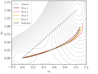
Figure 1: OptiBounce convergence on the two-field potential with $\delta=0.3$. For this test case the IPOPT solver converges in nine steps. We show the initial straight-line ansatz, the first four steps, and the solution at step nine.

Our objective in this section is to explore the performance and accuracy of the new algorithm on test potentials with multiple fields. We build our test cases using the form introduced in Athron et al. (2019b):

$$V_{n_{\phi}}=\bigg{(}\bigg{[}\sum_{i=1}^{n_{\phi}}c_{i}(\phi_{i}-1)^{2}\bigg{]}-\delta\bigg{)}\bigg{(}\sum_{i=1}^{n_{\phi}}\phi_{i}^{2}\bigg{)}$$ (34)

where the coefficients $c_{i}$ are given in appendix A. The two field case with $\delta=0.3$ is shown in figure 1. For $0<\delta<1$ this potential has a false vacuum at $(0,0)$ and a true vacuum in the vicinity of $(1,1)$. As $\delta\rightarrow 0$, the vacua approach degeneracy and the solution becomes thin-walled. In physical terms, this reflects the situation near the critical temperature when $(T-T_{C})/T_{C}\ll 1$. Figure 2 contrasts the different kinds of solutions obtained for large and small values of $\delta$.

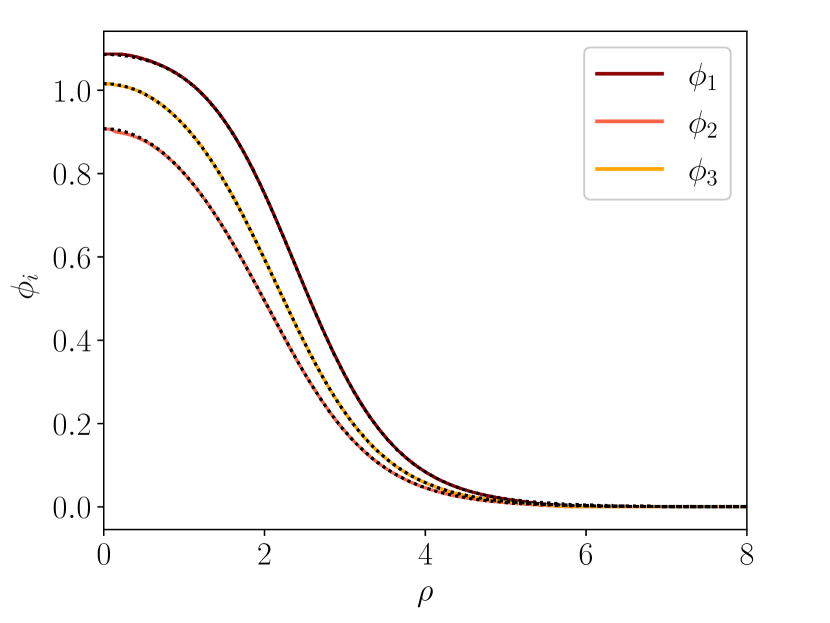
(a) $\delta=0.3$

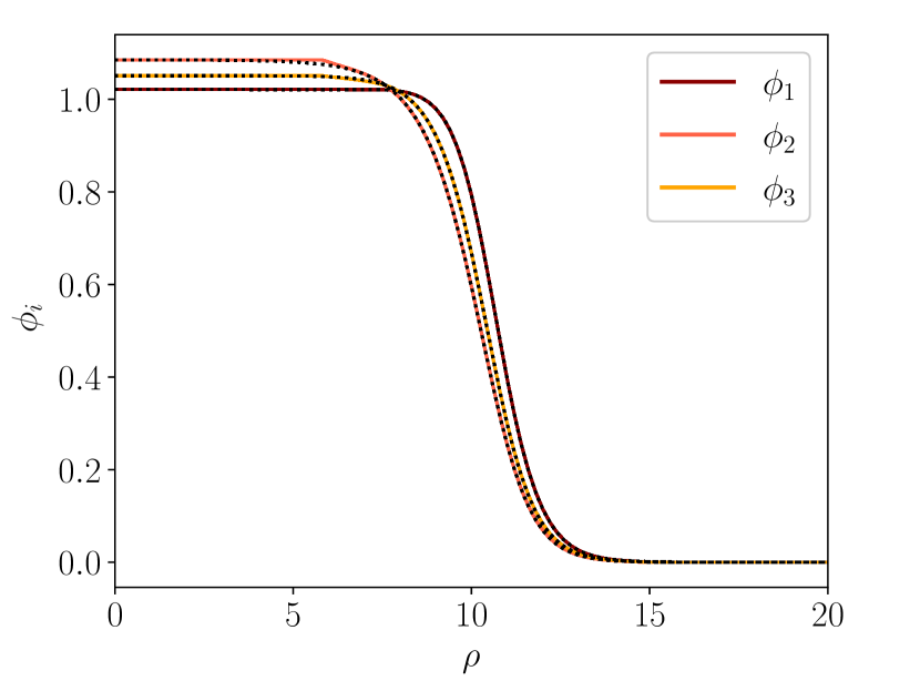
(b) $\delta=0.03$

Figure 2: Thick- and thin-walled solutions for the test potential 34 with $n_{\phi}=3$. Solution curves are shown for the OptiBounce algorithm (dashed) and FindBounce (solid).

As described in section II.3, our algorithm is optimised for quickly finding the nucleation temperature. Figure 3 models this kind of computation using the limit $\delta\rightarrow 0$ as a proxy for $T\rightarrow T_{C}$ on the $n_{\phi}=5$ test potential. Away from the thin-wall limit, we find that the per-point computation time is greatly reduced compared to CosmoTransitions and FindBounce. For smaller values of $\delta$ the computation time becomes comparable to the other two codes. As noted in section II.2, this corresponds to the regime where the bubble wall scale is smaller than the grid size. We consider this to be a defect of the discretisation scheme rather than the algorithm as a whole, and expect that an adaptive scheme would allow better performance in the thin-wall limit.

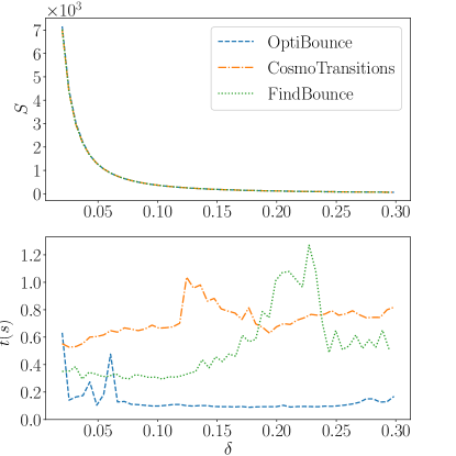
Figure 3: Action and timing data for the $n_{\phi}=5$ test potential with $\delta\in[0.02,0.3]$. For OptiBounce the number of collocation points per element was increased from $d=3$ to $d=7$ to improve accuracy in the thin wall limit. Note that the OptiBounce timings do not include the one-off setup cost, as this computation was shared between all instances of the calculation.

We also investigated the performance of the algorithm with larger numbers of fields up to $n_{\phi}=20$. To ensure consistency between different values of $n_{\phi}$ we chose values of $\delta$ such that the action was in the range $S\in[200,400]$, representing cases away from both the thick- and thin-walled limits. Table 1 presents the timings for each case along with comparisons to CosmoTransitions and FindBounce. In all cases the action obtained by the codes agrees to within $1\%$. For our algorithm the setup and solution times are reported separately. Considering the solution time only, we outperform the other codes for all values of $n_{\phi}$. If we also account for the setup time, for $n_{\phi}>13$ FindBounce is faster on some points. However, we emphasise that when finding nucleation temperatures the setup time is a one-off cost which implies that for a sufficiently large number of evaluations our algorithm should be more efficient.

$n_{\phi}$	$\delta$	Action (OB)	$\text{t}_{\text{setup}}$ (OB)	$\text{t}_{\text{sol}}$ (OB)	Action (FB)	$\text{t}_{\text{sol}}$ (FB)	Action (CT)	$\text{t}_{\text{sol}}$ (CT)
3	0.065	240.049	0.191	0.009	240.403	0.294	240.324	0.492
4	0.11	227.023	0.217	0.081	230.864	0.615	230.397	3.223
5	0.13	233.523	0.259	0.025	233.716	0.408	233.357	0.976
6	0.15	270.363	0.300	0.031	270.578	0.442	271.769	3.917
7	0.2	250.054	0.355	0.046	250.222	0.482	249.845	3.802
8	0.22	268.259	0.404	0.085	268.486	0.606	269.368	4.143
9	0.29	204.609	0.452	0.083	204.796	0.675	205.888	0.769
10	0.27	261.468	0.507	0.088	261.703	0.779	261.273	1.279
11	0.3	273.271	0.565	0.116	273.564	0.861	-	-
12	0.32	249.691	0.618	0.158	249.928	0.950	-	-
13	0.39	293.383	0.671	0.153	293.653	1.012	-	-
14	0.39	294.677	0.731	0.528	294.877	1.114	-	-
15	0.42	312.760	0.816	0.455	313.039	1.222	-	-
16	0.45	366.870	0.881	0.471	366.978	1.885	-	-
17	0.52	342.537	0.961	0.734	342.893	1.395	-	-
18	0.47	390.925	1.060	0.772	391.231	1.544	-	-
19	0.56	339.287	1.116	1.537	339.467	2.436	-	-
20	0.55	381.886	1.178	1.309	382.153	1.864	-	-

Table 1: Timing data and action for test potentials with up to $n_{\phi}=20$ fields. Results are shown for the OptiBounce algorithm, CosmoTransitions (CT) and FindBounce (FB). For OptiBounce we report the setup time $\text{t}_{\text{setup}}$ and solution time $\text{t}_{\text{sol}}$ separately, with the total runtime being $\text{t}_{\text{setup}}+\text{t}_{\text{sol}}$. CosmoTransitions results for $n_{\phi}>10$ are not reported as the code issues an error when there are more than 10 fields.

IV Conclusion

In this paper, we presented a new and efficient method for finding the bounce solution. The OptiBounce algorithm is based on Coleman, Glaser, and Martin’s original “reduced” action Coleman et al. (1978), which has a true minimum at a solution related to the bounce by a scale transform. We provided an analytic result showing that the scale transform is not even required to compute the bounce action (see equation 15, appendix A). To implement this method we designed a Legendre-Gauss collocation scheme to represent the bounce solution, yielding a large scale finite-dimensional optimisation problem over the collocation coefficients. Taking advantage of recent advances in large scale optimisation and automatic differentiation, we implemented the scheme using a CasADi-IPOPT stack to explore the accuracy and performance characteristics of OptiBounce. We were able to reproduce the results of the CosmoTransitions and FindBounce codes to within $O(1\%)$ on a set of test problems with 3-20 scalar fields. Our performance results suggest that the OptiBounce approach will be especially efficient for finding nucleation temperatures as the initial setup cost can be shared between executions. Neglecting this setup cost, our execution times are frequently orders of magnitude faster than the other codes we analysed.

Appendix A Derivation of optimisation algorithm

In this section we provide a derivation establishing that the algorithm described in section II.1 recovers the bounce action and field profile via equations 15 and 16. Our starting point is the “reduced problem” defined by Coleman, Glaser, and Martin Coleman et al. (1978). Recall that the set $\mathbf{\Phi}$ contains all field profiles satisfying the boundary conditions $\dot{\phi}_{i}(0)=0$, $\lim_{\rho\to\infty}\phi_{i}(\rho)=0$, $1\leq i\leq n_{\phi}$. For each $\bm{\phi}\in\mathbf{\Phi}$, we consider the scale transformation $\bm{\phi}_{\sigma}(\rho)=\bm{\phi}(\sigma^{-1}\rho)$ for some $\sigma>0$. Firstly, the action transforms as:

$$S_{E}[\bm{\phi}_{\sigma}(\rho)]=\sigma^{D-2}T[\bm{\phi}(\rho)]+\sigma^{D}V[\bm{\phi}(\rho)].$$ (35)

Since the bounce solution $\bm{\phi}^{B}$ makes $S_{E}$ stationary, this variation should vanish around $\sigma=1$:

$$\frac{dS_{E}[\bm{\phi}_{\sigma}^{B}(\rho)]}{d\sigma}\bigg{|}_{\sigma=1}=(D-2)T[\bm{\phi}^{B}(\rho)]+DV[\bm{\phi}^{B}(\rho)]=0,$$ (36)

yielding the relation

$$V=\frac{2-D}{D}T.$$ (37)

Since $T>0$, for $D\geq 2$ this implies $V[\bm{\phi}^{B}]<0$. Moreover, if the bounce solution exists then the level set:

$$\bm{\Phi}_{V_{0}}\equiv\{\bm{\phi}\in\bm{\Phi}:V[\bm{\phi}]=V_{0}\}$$ (38)

is not empty for any $V_{0}<0$ since clearly $V[\bm{\phi}^{B}_{\sigma}]=V_{0}$ for some $\sigma>0$. Therefore the minimizer:

$$\bm{\phi}^{*}\equiv\operatorname*{arg\,min}_{\bm{\phi}\in\Phi_{V_{0}}}T[\bm{\phi}(\rho)]$$ (39)

must exist. If we implement the constraint $V[\bm{\phi}]=V_{0}$ with a Lagrange multiplier $\lambda$, $\bm{\phi}^{*}$ is a stationary point of the augmented Lagrangian:

$$S_{E}[\bm{\phi}(\rho),\lambda]=T[\bm{\phi}(\rho)]+\lambda(V[\bm{\phi}(\rho)]-V_{0}).$$ (40)

In fact, if we relax the constraint and introduce the optimal Lagrange multiplier $\lambda_{*}$, it is also a stationary point of:

$$S_{\lambda_{*}}[\bm{\phi}(\rho)] =T[\bm{\phi}(\rho)]+\lambda_{*}V[\bm{\phi}(\rho)]$$ (41)

$$=\int_{0}^{\infty}d\rho\rho^{D-1}\bigg{[}\frac{1}{2}|\dot{\bm{\phi}}|^{2}+\lambda_{*}V(\bm{\phi})\bigg{]},$$ (42)

and so has equations of motion:

$$\ddot{\phi^{*}_{i}}+\frac{D-1}{\rho}\dot{\phi^{*}_{i}}=\lambda_{*}\frac{\partial V}{\partial\phi^{*}_{i}}.$$ (43)

This means that we can recover the bounce solution by a scale transform $\bm{\phi}^{B}(\rho)=\bm{\phi}^{*}(\rho/\sqrt{\lambda_{*}})$, since then:

$$\ddot{\phi^{B}_{i}}+\frac{D-1}{\rho}\dot{\phi^{B}_{i}}=\frac{\partial V}{\partial\phi^{B}_{i}}.$$ (44)

Moreover, since $\bm{\phi}^{B}$ is a stationary point of $S_{E}[\bm{\phi}(\rho)]$ we can directly obtain the action by inverting equation 37:

$$S_{E}[\bm{\phi}^{B}(\rho)] =\frac{2}{2-D}V[\bm{\phi}^{*}(\rho/\sqrt{\lambda_{*}})]$$ (45)

$$=\frac{2}{2-D}\lambda_{*}^{\frac{D}{2}}V[\bm{\phi}^{*}(\rho)]$$ (46)

$$=\frac{2\lambda_{*}^{\frac{d}{2}}V_{0}}{2-D}.$$ (47)

Alternatively, from equation 35 we have:

$$T[\bm{\phi}^{B}(\rho)]=\lambda_{*}^{1-\frac{D}{2}}T[\bm{\phi}^{B}(\rho/\sqrt{\lambda_{*}})]\equiv\lambda_{*}^{1-\frac{D}{2}}T_{0}.$$ (48)

Inserting equation 37 into $S=T+V$ then gives:

$$S_{E}[\bm{\phi}^{B}(\rho)]=\frac{2}{D}T[\bm{\phi}^{B}(\rho)]=\frac{2\lambda_{*}^{\frac{D}{2}-1}T_{0}}{D}.$$ (49)

Equality between the two expressions for $S_{E}[\bm{\phi}^{B}(\rho)]$ means we can write $\lambda_{*}$ in terms of $T_{0}/V_{0}$:

$$\lambda_{*}=\bigg{(}\frac{2-D}{D}\bigg{)}\frac{T_{0}}{V_{0}}.$$ (50)

This means that we can express $S_{E}[\bm{\phi}^{B}(\rho)]$ in terms of $T_{0}$, $V_{0}$ and $D$ only:

$$S[\bm{\phi}(\rho)]=\bigg{[}\bigg{(}\frac{2-D}{D}\bigg{)}\frac{T_{0}}{V_{0}}\bigg{]}^{\frac{D}{2}-1}\frac{2T_{0}}{D}.$$ (51)

$n_{\phi}$	$\delta$	$c_{i}$
3	0.065	0.684373, 0.181928, 0.295089
4	0.11	0.534808, 0.77023, 0.838912, 0.00517238
5	0.13	0.4747, 0.234808, 0.57023, 0.138912, 0.517238
6	0.1	0.34234, 0.4747, 0.234808, 0.57023, 0.138912, 0.517238
7	0.2	0.5233, 0.34234, 0.4747, 0.234808, 0.57023, 0.138912, 0.517238
8	0.22	0.2434, 0.5233, 0.34234, 0.4747, 0.234808, 0.57023, 0.138912, 0.51723
9	0.29	0.21, 0.24, 0.52, 0.34, 0.47, 0.23, 0.57, 0.14, 0.52
10	0.27	0.12, 0.21, 0.24, 0.52, 0.34, 0.47, 0.23, 0.57, 0.14, 0.52
11	0.3	0.23, 0.21, 0.21, 0.24, 0.52, 0.34, 0.47, 0.23, 0.57, 0.14, 0.52
12	0.32	0.12, 0.11, 0.12, 0.21, 0.24, 0.52, 0.34, 0.47, 0.23, 0.57, 0.14, 0.52
13	0.39	0.54, 0.47, 0.53, 0.28, 0.35, 0.27, 0.42, 0.59, 0.33, 0.16, 0.38, 0.35, 0.17
14	0.39	0.39, 0.23, 0.26, 0.40, 0.11, 0.42, 0.41, 0.27, 0.42, 0.54, 0.18, 0.59, 0.13, 0.29
15	0.42	0.21, 0.22, 0.22, 0.23, 0.39, 0.55, 0.43, 0.12, 0.16, 0.58, 0.25, 0.50, 0.45, 0.35, 0.45
16	0.45	0.42, 0.34, 0.43, 0.22, 0.59, 0.41, 0.58, 0.41, 0.26, 0.45, 0.16, 0.31, 0.39, 0.57, 0.43, 0.10
17	0.52	0.24, 0.35, 0.39, 0.56, 0.37, 0.41, 0.52, 0.31, 0.52, 0.22, 0.58, 0.39, 0.39, 0.17, 0.46, 0.30, 0.37
18	0.47	0.18, 0.17, 0.30, 0.22, 0.38, 0.48, 0.11, 0.49, 0.43, 0.47, 0.21, 0.29, 0.32, 0.36, 0.30, 0.56, 0.46, 0.42
19	0.56	0.40, 0.14, 0.10, 0.43, 0.39, 0.27, 0.33, 0.59, 0.48, 0.36, 0.24, 0.28, 0.51, 0.59, 0.40, 0.39, 0.24, 0.35, 0.20
20	0.55	0.42, 0.11, 0.47, 0.13, 0.16, 0.24, 0.58, 0.53, 0.38, 0.44, 0.18, 0.46, 0.47, 0.27, 0.53, 0.24, 0.33, 0.40, 0.32, 0.29

Table 2: Coefficients used to generate the timing results in table 1 with the potential defined in equation 34. For $3\leq n_{\phi}\leq 8$, the $c_{i}$ are taken from Athron et al. (2019b), with the remainder for $n_{\phi}\geq 9$ from Guada et al. (2020).

References

- Kakizaki et al. (2015) Mitsuru Kakizaki, Shinya Kanemura, and Toshinori Matsui, “Gravitational waves as a probe of extended scalar sectors with the first order electroweak phase transition,” Physical Review D 92, 115007 (2015), arXiv:1509.08394 .
- Balázs et al. (2017) Csaba Balázs, Andrew Fowlie, Anupam Mazumdar, and Graham A. White, “Gravitational waves at aLIGO and vacuum stability with a scalar singlet extension of the standard model,” Physical Review D 95, 043505 (2017).
- Papaefstathiou and White (2020) Andreas Papaefstathiou and Graham White, “The Electro-Weak Phase Transition at Colliders: Confronting Theoretical Uncertainties and Complementary Channels,” (2020).
- Alves et al. (2019) Alexandre Alves, Tathagata Ghosh, Huai-Ke Guo, Kuver Sinha, and Daniel Vagie, “Collider and Gravitational Wave Complementarity in Exploring the Singlet Extension of the Standard Model,” Journal of High Energy Physics 2019, 52 (2019), arXiv:1812.09333 .
- Athron et al. (2019a) Peter Athron, Csaba Balazs, Andrew Fowlie, Giancarlo Pozzo, Graham White, and Yang Zhang, “Strong first-order phase transitions in the NMSSM — a comprehensive survey,” Journal of High Energy Physics 2019, 151 (2019a).
- Jiang et al. (2016) Minyuan Jiang, Ligong Bian, Weicong Huang, and Jing Shu, “Impact of a complex singlet: Electroweak baryogenesis and dark matter,” Physical Review D 93 (2016), 10.1103/PhysRevD.93.065032.
- Dorsch et al. (2017) G. C. Dorsch, S. J. Huber, T. Konstandin, and J. M. No, “A Second Higgs Doublet in the Early Universe: Baryogenesis and Gravitational Waves,” Journal of Cosmology and Astroparticle Physics 2017, 052–052 (2017), arXiv:1611.05874 .
- Kuzmin et al. (1985) V. A. Kuzmin, V. A. Rubakov, and M. E. Shaposhnikov, “On the Anomalous Electroweak Baryon Number Nonconservation in the Early Universe,” Phys.Lett. 155B, 36 (1985).
- Shaposhnikov (1987) M. E. Shaposhnikov, “Baryon asymmetry of the universe in standard electroweak theory,” Nuclear Physics B 287, 757–775 (1987).
- Morrissey and Ramsey-Musolf (2012) David E. Morrissey and Michael J. Ramsey-Musolf, “Electroweak baryogenesis,” New Journal of Physics 14, 125003 (2012), arXiv:1206.2942 .
- White (2016) Graham Albert White, A Pedagogical Introduction to Electroweak Baryogenesis, edited by Morgan & Claypool Publishers and Institute of Physics (Great Britain), IOP (Series). Release 3. (San Rafael [California] (40 Oak Drive, San Rafael, CA, 94903, USA): Morgan & Claypool Publishers, 2016).
- Witten (1984) Edward Witten, “Cosmic separation of phases,” Physical Review D 30, 272–285 (1984).
- Hogan (1986) C. J. Hogan, “Gravitational radiation from cosmological phase transitions,” Monthly Notices of the Royal Astronomical Society 218, 629–636 (1986).
- Cutting et al. (2018) Daniel Cutting, Mark Hindmarsh, and David J. Weir, “Gravitational waves from vacuum first-order phase transitions: From the envelope to the lattice,” Physical Review D 97, 123513 (2018).
- Caprini et al. (2020) Chiara Caprini, Mikael Chala, Glauber C. Dorsch, Mark Hindmarsh, Stephan J. Huber, Thomas Konstandin, Jonathan Kozaczuk, Germano Nardini, Jose Miguel No, Kari Rummukainen, Pedro Schwaller, Geraldine Servant, Anders Tranberg, and David J. Weir, “Detecting gravitational waves from cosmological phase transitions with LISA: An update,” Journal of Cosmology and Astroparticle Physics 2020, 024–024 (2020).
- Sigl et al. (1997) Guenter Sigl, Angela Olinto, and Karsten Jedamzik, “Primordial Magnetic Fields from Cosmological First Order Phase Transitions,” Physical Review D 55, 4582–4590 (1997), arXiv:astro-ph/9610201 .
- Tevzadze et al. (2012) Alexander G. Tevzadze, Leonard Kisslinger, Axel Brandenburg, and Tina Kahniashvili, “Magnetic Fields from QCD Phase Transitions,” The Astrophysical Journal 759, 54 (2012), arXiv:1207.0751 .
- Ellis et al. (2019a) John Ellis, Malcolm Fairbairn, Marek Lewicki, Ville Vaskonen, and Alastair Wickens, “Intergalactic magnetic fields from first-order phase transitions,” Journal of Cosmology and Astroparticle Physics 2019, 019 (2019a).
- Aazami and Easther (2006) Amir Aazami and Richard Easther, “Cosmology From Random Multifield Potentials,” Journal of Cosmology and Astroparticle Physics 2006, 013–013 (2006), arXiv:hep-th/0512050 .
- Greene et al. (2013) Brian Greene, David Kagan, Ali Masoumi, Dhagash Mehta, Erick J. Weinberg, and Xiao Xiao, “Tumbling through a landscape: Evidence of instabilities in high-dimensional moduli spaces,” Physical Review D 88 (2013), 10.1103/PhysRevD.88.026005, arXiv:1303.4428 .
- Dine and Paban (2015) Michael Dine and Sonia Paban, “Tunneling in theories with many fields,” Journal of High Energy Physics 2015, 88 (2015).
- Masoumi and Vilenkin (2016) Ali Masoumi and Alexander Vilenkin, “Vacuum statistics and stability in axionic landscapes,” Journal of Cosmology and Astroparticle Physics 2016, 054–054 (2016).
- Coleman (1977) Sidney Coleman, “Fate of the false vacuum: Semiclassical theory,” Physical Review D 15, 2929–2936 (1977).
- Callan and Coleman (1977) Curtis G. Callan and Sidney Coleman, “Fate of the false vacuum. II. First quantum corrections,” Physical Review D 16, 1762–1768 (1977).
- Linde (1981) A. D. Linde, “Fate of the false vacuum at finite temperature: Theory and applications,” Physics Letters B 100, 37–40 (1981).
- Ellis et al. (2019b) John Ellis, Marek Lewicki, and José Miguel No, “On the Maximal Strength of a First-Order Electroweak Phase Transition and its Gravitational Wave Signal,” Journal of Cosmology and Astroparticle Physics 2019, 003–003 (2019b), arXiv:1809.08242 .
- Maziashvili (2003) Michael Maziashvili, “Uniqueness of a Negative Mode About a Bounce Solution,” Journal of Physics A: Mathematical and General 36, L463–L466 (2003), arXiv:hep-th/0212283 .
- Kusenko (1995) Alexander Kusenko, “Improved Action Method for Analysing Tunneling in Quantum Field Theory,” Physics Letters B 358, 51–55 (1995), arXiv:hep-ph/9504418 .
- John (1999) P. John, “Bubble Wall Profiles With More Than One Scalar Field: A Numerical Approach,” Physics Letters B 452, 221–226 (1999), arXiv:hep-ph/9810499 .
- Konstandin and Huber (2006) Thomas Konstandin and Stephan J. Huber, “Numerical Approach to Multi Dimensional Phase Transitions,” Journal of Cosmology and Astroparticle Physics 2006, 021–021 (2006), arXiv:hep-ph/0603081 .
- Park (2011) Jae-hyeon Park, “Constrained potential method for false vacuum decays,” Journal of Cosmology and Astroparticle Physics 2011, 023–023 (2011), arXiv:1011.4936 .
- Espinosa and Konstandin (2019) José Ramón Espinosa and Thomas Konstandin, “A Fresh Look at the Calculation of Tunneling Actions in Multi-Field Potentials,” Journal of Cosmology and Astroparticle Physics 2019, 051–051 (2019), arXiv:1811.09185 .
- Guada et al. (2019) Victor Guada, Alessio Maiezza, and Miha Nemevšek, “Multifield polygonal bounces,” Physical Review D 99, 056020 (2019).
- Piscopo et al. (2019) Maria Piscopo, Michael Spannowsky, and Philip Waite, “Solving differential equations with neural networks: Applications to the calculation of cosmological phase transitions,” Physical Review D 100 (2019), 10.1103/PhysRevD.100.016002.
- Sato (2020) Ryosuke Sato, “Simple gradient flow equation for the bounce solution,” Physical Review D 101, 016012 (2020).
- Chigusa et al. (2020) So Chigusa, Takeo Moroi, and Yutaro Shoji, “Bounce Configuration from Gradient Flow,” Physics Letters B 800, 135115 (2020), arXiv:1906.10829 .
- Wainwright (2012) Carroll L. Wainwright, “CosmoTransitions: Computing cosmological phase transition temperatures and bubble profiles with multiple fields,” Computer Physics Communications 183, 2006–2013 (2012).
- Masoumi et al. (2017) Ali Masoumi, Ken D. Olum, and Benjamin Shlaer, “Efficient numerical solution to vacuum decay with many fields,” Journal of Cosmology and Astroparticle Physics 2017, 051 (2017).
- Athron et al. (2019b) Peter Athron, Csaba Balázs, Michael Bardsley, Andrew Fowlie, Dylan Harries, and Graham White, “Bubbleprofiler: Finding the field profile and action for cosmological phase transitions,” Computer Physics Communications 244, 448–468 (2019b).
- Akula et al. (2016) Sujeet Akula, Csaba Balázs, and Graham A. White, “Semi-analytic techniques for calculating bubble wall profiles,” The European Physical Journal C 76, 681 (2016).
- Guada et al. (2020) Victor Guada, Miha Nemevšek, and Matevž Pintar, “FindBounce: Package for multi-field bounce actions,” Computer Physics Communications 256, 107480 (2020).
- Sato (2021) Ryosuke Sato, “SimpleBounce: A simple package for the false vacuum decay,” Computer Physics Communications 258, 107566 (2021).
- Andersson et al. (2019) Joel A. E. Andersson, Joris Gillis, Greg Horn, James B. Rawlings, and Moritz Diehl, “CasADi: A software framework for nonlinear optimization and optimal control,” Mathematical Programming Computation 11, 1–36 (2019).
- Wächter and Biegler (2006) Andreas Wächter and Lorenz T. Biegler, “On the implementation of an interior-point filter line-search algorithm for large-scale nonlinear programming,” Mathematical Programming 106, 25–57 (2006).
- Coleman et al. (1978) S. Coleman, V. Glaser, and A. Martin, “Action minima among solutions to a class of Euclidean scalar field equations,” Communications in Mathematical Physics 58, 211–221 (1978).
- Garg et al. (2011) Divya Garg, Michael A. Patterson, Camila Francolin, Christopher L. Darby, Geoffrey T. Huntington, William W. Hager, and Anil V. Rao, “Direct trajectory optimization and costate estimation of finite-horizon and infinite-horizon optimal control problems using a Radau pseudospectral method,” Computational Optimization and Applications 49, 335–358 (2011).
- Huntington and Rao (2007) Geoffrey T. Huntington and Anil V. Rao, “A Comparison between Global and Local Orthogonal Collocation Methods for Solving Optimal Control Problems,” in 2007 American Control Conference (2007) pp. 1950–1957.
- Note (1) On the same number of points, the Newton-Cotes quadrature is of exactness .
- Liu et al. (2015) Fengjin Liu, William W. Hager, and Anil V. Rao, “Adaptive mesh refinement method for optimal control using nonsmoothness detection and mesh size reduction,” Journal of the Franklin Institute 352, 4081–4106 (2015).