The Mass Ratio Distribution of Tertiary Induced Binary Black Hole Mergers

Abstract

Many proposed scenarios for black hole (BH) mergers involve a tertiary companion that induces von Zeipel-Lidov-Kozai (ZLK) eccentricity cycles in the inner binary. An attractive feature of such mechanisms is the enhanced merger probability when the octupole-order effects, also known as the eccentric Kozai mechanism, are important. This can be the case when the tertiary is of comparable mass to the binary components. Since the octupole strength [$\propto(1-q)/(1+q)$] increases with decreasing binary mass ratio $q$, such ZLK-induced mergers favor binaries with smaller mass ratios. We use a combination of numerical and analytical approaches to fully characterize the octupole-enhanced binary BH mergers and provide semi-analytical criteria for efficiently calculating the strength of this enhancement. We show that for hierarchical triples with semi-major axis ratio $a/a_{\rm out}\gtrsim 0.01$–$0.02$, the binary merger fraction can increase by a large factor (up to $\sim 20$) as $q$ decreases from unity to $0.2$. The resulting mass ratio distribution for merging binary BHs produced in this scenario is in tension with the observed distribution obtained by the LIGO/VIRGO collaboration, although significant uncertainties remain about the initial distribution of binary BH masses and mass ratios.

1 Introduction

The $50$ or so black hole (BH) binary mergers detected by the LIGO/VIRGO collaboration to date (Abbott et al., 2020a) continue to motivate theoretical studies of their formation channels. These range from the traditional isolated binary evolution, in which mass transfer and friction in the common envelope phase cause the binary orbit to decay sufficiently that it subsequently merges via emission of gravitational waves (GWs) (e.g., Lipunov et al., 1997, 2017; Podsiadlowski et al., 2003; Belczynski et al., 2010, 2016; Dominik et al., 2012, 2013; Dominik et al., 2015), to various flavors of dynamical formation channels that involve either strong gravitational scatterings in dense clusters (e.g., Portegies Zwart & McMillan, 2000; O’leary et al., 2006; Miller & Lauburg, 2009; Banerjee et al., 2010; Downing et al., 2010; Ziosi et al., 2014; Rodriguez et al., 2015; Samsing & Ramirez-Ruiz, 2017; Samsing & D’Orazio, 2018; Rodriguez et al., 2018; Gondán et al., 2018) or mergers in isolated triple and quadruple systems induced by distant companions (e.g., Miller & Hamilton, 2002; Wen, 2003; Antonini & Perets, 2012a; Antonini et al., 2017; Silsbee & Tremaine, 2017; Liu & Lai, 2017, 2018; Randall & Xianyu, 2018a, b; Hoang et al., 2018; Fragione & Kocsis, 2019; Fragione & Loeb, 2019; Liu & Lai, 2019; Liu et al., 2019a, b; Liu & Lai, 2020; Liu & Lai, 2021).

Given the large number of merger events to be detected in the coming years, it is important to search for observational signatures to distinguish various BH binary formation channels. The masses of merging BHs obviously carry important information. The recent detection of BH binary systems with component masses in the mass gap (such in GW190521) suggests that some kinds of “hierarchical mergers” may be needed to explain these exceptional events (Abbott et al., 2020b; see Liu & Lai, 2021 for examples of such “hierarchical mergers” in stellar multiples). Another possible indicator is merger eccentricity: previous studies find that dynamical binary-single interactions in dense clusters (e.g., Samsing & Ramirez-Ruiz, 2017; Rodriguez et al., 2018; Samsing & D’Orazio, 2018; Fragione & Bromberg, 2019) or in galactic triples (Silsbee & Tremaine, 2017; Antonini et al., 2017; Fragione & Loeb, 2019; Liu et al., 2019a) may lead to BH binaries that enter the LIGO band with modest eccentricities. The third possible indicator is the spin-orbit misalignment of the binary. In particular, the mass-weighted projection of the BH spins,

$$\chi_{\rm eff}=\frac{m_{1}\boldsymbol{\chi}_{1}+m_{2}\boldsymbol{\chi}_{2}}{m_{1}+m_{2}}\cdot\hat{\mathbf{L}},$$ (1)

can be measured through the binary inspiral waveform [here, $m_{1,2}$ is the BH mass, $\boldsymbol{\chi}_{1,2}=c\boldsymbol{S}_{1,2}/(Gm_{1,2}^{2})$ is the dimensionless BH spin, and $\hat{\mathbf{L}}$ is the unit orbital angular momentum vector of the binary]. Different formation histories yield different distributions of $\chi_{\rm eff}$ (Liu & Lai, 2017, 2018; Antonini et al., 2018; Rodriguez et al., 2018; Gerosa et al., 2018; Liu et al., 2019a; Su et al., 2021).

The fourth possible indicator of BH binary formation mechanisms is the distribution of masses and mass ratios of merging BHs. In Fig. 1, we show the distribution of the mass ratio $q\equiv m_{2}/m_{1}$, where $m_{1}\geq m_{2}$, for all LIGO/VIRGO binaries detected as of the O3a data release (Abbott et al., 2020a). The distribution distinctly peaks around $q\sim 0.7$. BH binaries formed via isolated binary evolution are generally expected to have $q\gtrsim 0.5$ (Belczynski et al., 2016; Olejak et al., 2020). On the other hand, dynamical formation channels may produce a larger variety of distributions for the binary mass ratio (e.g., Rodriguez et al., 2016; Silsbee & Tremaine, 2017; Fragione & Kocsis, 2019).

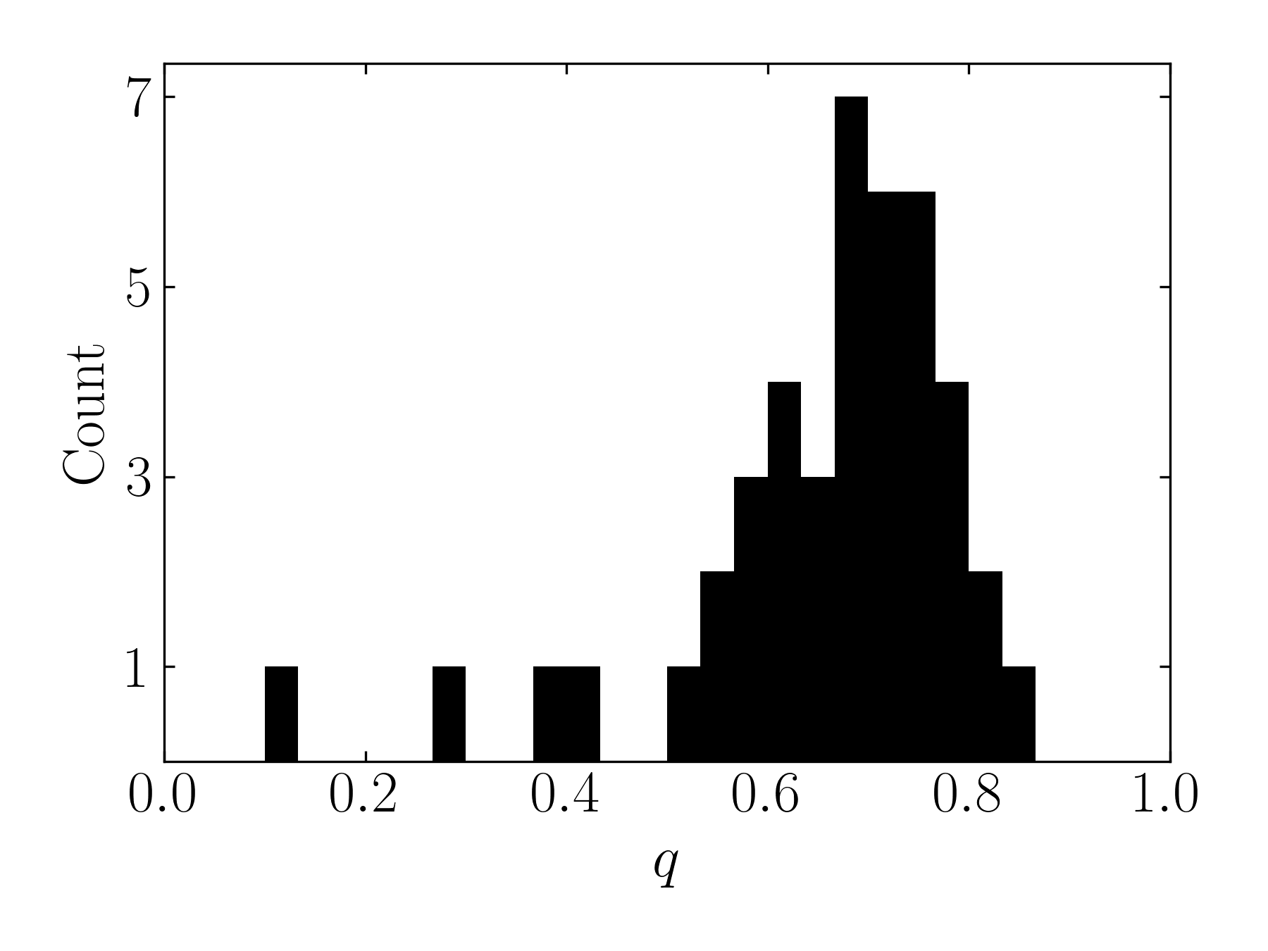
Figure 1: Histogram of the mass ratios $q\equiv m_{2}/m_{1}$ of binary BH mergers in the O3a data release, excluding the two NS-NS mergers but including GW190814, whose $2.5M_{\odot}$ secondary may be a BH (Abbott et al., 2020a).

In this paper, we study in detail the mass ratio distribution for BH mergers induced by tertiary companions in isolated triple systems. In this scenario, a tertiary BH on a sufficiently inclined (outer) orbit induces phases of extreme eccentricity in the inner binary via the von Zeipel-Lidov-Kozai (ZLK;von Zeipel, 1910; Lidov, 1962; Kozai, 1962) effect, leading to efficient gravitational radiation and orbital decay. While the original ZLK effect relies on the leading-order, quadrupolar gravitational perturbation from the tertiary on the inner binary, the octupole order terms can become important (sometimes known as the eccentric Kozai mechanism, e.g. Naoz, 2016) when the triple system is mildly hierarchical, the outer orbit is eccentric ($e_{\rm out}\neq 0$) and the inner binary BHs have unequal masses (e.g., Ford et al., 2000; Blaes et al., 2002; Lithwick & Naoz, 2011; Liu et al., 2015). The strength of the octupole effect depends on the dimensionless parameter

$$\epsilon_{\rm oct}=\frac{m_{1}-m_{2}}{m_{1}+m_{2}}\frac{a}{a_{\rm out}}\frac{e_{\rm out}}{1-e_{\rm out}^{2}}.$$ (2)

where $a,a_{\rm out}$ are the semi-major axes of the inner and outer binaries, respectively. Previous studies have shown that the octupole terms generally increase the inclination window for extreme eccentricity excitation, and thus enhance the rate of successful binary mergers (Liu & Lai, 2018). As $\epsilon_{\rm oct}\propto(1-q)/(1+q)$ increases with decreasing $q$, we expect that ZLK-induced BH mergers favor binaries with smaller mass ratios. The main goal of this paper is to quantify the dependence of the merger fraction/probability on $q$, using a combination of analytical and numerical calculations. We focus on the cases where the tertiary mass is comparable to the binary BH masses. When the tertiary mass $m_{3}$ is much larger than $m_{12}=m_{1}+m_{2}$ (as in the case of a supermassive BH tertiary), dynamical stability of the triple requires $a_{\rm out}(1-e_{\rm out})/[a(1+e)]\gtrsim 3.7(m_{3}/m_{12})^{1/3}\gg 1$ (Kiseleva et al., 1996), which implies that the octupole effect is negligible.

This paper is organized as follows. In Section 2, we review some analytical results of ZLK oscillations and examine how the octupole terms affect the inclination window and probability for extreme eccentricity excitation. In Section 3, we study tertiary-induced BH mergers using a combination of numerical and analytical approaches. We propose new semi-analytical criteria (Section 3.2) that allow us to determine, without full numerical integration, whether an initial BH binary can undergo a “one-shot merger” or a more gradual merger induced by the octupole effect of an tertiary. In Section 4, we calculate the merger fraction as a function of mass ratio for some representative triple systems. In Section 5, we study the mass ratio distribution of the initial BH binaries based on the properties of main-sequence (MS) stellar binaries and the MS mass to BH mass mapping. Using the result of Section 4, we illustrate how the final merging BH binary mass distribution may be influenced by the octupole effect for tertiary-induced mergers. We summarize our results and their implications in Section 6.

2 Von Zeipel-Lidov-Kozai (ZLK) Oscillations: Analytical Results

Consider two BHs orbiting each other with masses $m_{1}$ and $m_{2}$ on a orbit with semi-major axis $a$, eccentricity $e$, and angular momentum $\mathbf{L}$. An external, tertiary BH of mass $m_{3}$ orbits this inner binary with semi-major axis $a_{\rm out}$, eccentricity $e_{\rm out}$, and angular momentum $\mathbf{L}_{\rm out}$. The reduced masses of the inner and outer binaries are $\mu\equiv m_{1}m_{2}/m_{12}$ and $\mu_{\rm out}\equiv m_{12}m_{3}/m_{123}$ respectively, where $m_{12}=m_{1}+m_{2}$ and $m_{123}=m_{12}+m_{3}$. These two binary orbits are further described by three angles: the inclinations $i$ and $i_{\rm out}$, the arguments of pericenters $\omega$ and $\omega_{\rm out}$, and the longitudes of the ascending nodes $\Omega$ and $\Omega_{\rm out}$. These angles are defined in a coordinate system where the $z$ axis is aligned with the total angular momentum $\mathbf{J}=\mathbf{L}+\mathbf{L}_{\rm out}$ (i.e., the invariant plane is perpendicular to $\mathbf{J}$). The mutual inclination between the two orbits is denoted $I\equiv i+i_{\rm out}$. Note that $\Omega_{\rm out}=\Omega+180^{\circ}$.

To study the evolution of the inner binary under the influence of the tertiary BH, we use the double-averaged secular equations of motion, including the interactions between the inner binary and the tertiary up to the octupole level of approximation as given by Liu et al. (2015). Throughout this paper, we restrict to hierarchical triple systems where the double-averaged secular equations are valid – systems with relatively small $a_{\rm out}/a$ may require solving the single-averaged equations of motion or direct N-body integration (see Antonini & Perets, 2012b; Antonini et al., 2014; Luo et al., 2016; Lei et al., 2018; Liu & Lai, 2019; Liu et al., 2019a; Hamers, 2020a). For the remainder of this section, we include general relativistic apsidal precession of the inner binary, a first order post-Newtonian (1PN) effect, but omit the emission of GWs, a 2.5PN effect – this will be considered in Section 3. We group the results by increasing order of approximation, starting by ignoring the octupole-order effects entirely.

2.1 Quadrupole Order

At the quadrupole order, the tertiary induces eccentricity oscillations in the inner binary on the characteristic timescale

$$t_{\rm ZLK}=\frac{1}{n}\frac{m_{12}}{m_{3}}\left(\frac{a_{\rm out,eff}}{a}\right)^{3},$$ (3)

where $n\equiv\sqrt{Gm_{12}/a^{3}}$ is the mean motion of the inner binary, and $a_{\rm out,eff}\equiv a_{\rm out}\sqrt{1-e_{\rm out}^{2}}$. During these oscillations, there are two conserved quantities, the total energy and the total orbital angular momentum. Through some manipulation, the total angular momentum can be written in terms of the conserved quantity $K$ given by

$$K\equiv j(e)\cos I-\frac{\eta}{2}e^{2}.$$ (4)

Here, $j(e)\equiv\sqrt{1-e^{2}}$ and $\eta$ is the ratio of the magnitudes of the angular momenta at zero inner binary eccentricity:

$$\eta\equiv\left(\frac{L}{L_{\rm out}}\right)_{e=0}=\frac{\mu}{\mu_{\rm out}}\left[\frac{m_{12}a}{m_{123}a_{\rm out}(1-e_{\rm out}^{2})}\right]^{1/2}.$$ (5)

Note that when $\eta=0$, $K$ reduces to the classical “Kozai constant”, $K=j(e)\cos I$.

The maximum eccentricity $e_{\max}$ attained in these ZLK oscillations can be computed analytically at the quadrupolar order. It depends on the “competition” between the 1PN apsidal precession rate $\dot{\omega}_{\rm GR}$ and the ZLK rate $t_{\rm ZLK}^{-1}$. The relevant dimensionless parameter is

$$\epsilon_{\rm GR}\equiv\left(\dot{\omega}_{\rm GR}t_{\rm ZLK}\right)_{e=0}=\frac{3Gm_{12}}{c^{2}}\frac{m_{12}}{m_{3}}\frac{a_{\rm out,eff}^{3}}{a^{4}}.$$ (6)

It can then be shown that, for an initially circular inner binary, $e_{\max}$ is related to the initial mutual inclination $I_{\rm 0}$ by (Liu et al., 2015; Anderson et al., 2016):

$$\frac{3}{8}\frac{j^{2}(e_{\max})-1}{j^{2}(e_{\max})}\Big{[} 5\left(\cos I_{0}+\frac{\eta}{2}\right)^{2}-\left(3+4\eta\cos I_{0}+\frac{9}{4}\eta^{2}\right)j^{2}(e_{\max})$$

$$+\eta^{2}j^{4}(e_{\max})\Big{]}+\epsilon_{\rm GR}\left[1-\frac{1}{j(e_{\max})}\right]=0.$$ (7)

In the limit $\eta\to 0$ and $\epsilon_{\rm GR}\to 0$, we recover the well-known result $e_{\max}=\sqrt{1-(5/3)\cos^{2}I_{0}}$. For general $\eta$, $e_{\max}$ attains its limiting value $e_{\lim}$ when $I_{\rm 0}=I_{\rm 0,\lim}$, where (see also Hamers, 2020b)

$$\cos I_{\rm 0,\lim}=\frac{\eta}{2}\left[\frac{4}{5}j^{2}(e_{\lim})-1\right].$$ (8)

Note that $I_{\rm 0,\lim}\geq 90^{\circ}$ with equality only when $\eta=0$. Substituting Eq. (8) into Eq. (7), we find that $e_{\lim}$ satisfies

$$\frac{3}{8}\left[j^{2}(e_{\lim})-1\right] \left[-3+\frac{\eta^{2}}{4}\left(\frac{4}{5}j^{2}(e_{\lim})-1\right)\right]$$

$$+\epsilon_{\rm GR}\left[1-\frac{1}{j(e_{\lim})}\right]=0.$$ (9)

On the other hand, eccentricity excitation ($e_{\max}\geq 0$) is only possible when $(\cos I_{\rm 0})_{-}\leq\cos I_{\rm 0}\leq(\cos I_{\rm 0})_{+}$ where

$$\left(\cos I_{\rm 0}\right)_{\pm}=\frac{1}{10}\left(-\eta\pm\sqrt{\eta^{2}+60-\frac{80}{3}\epsilon_{\rm GR}}\right).$$ (10)

For $I_{\rm 0}$ outside of this range, no eccentricity excitation is possible. This condition reduces to the well-known $\cos^{2}I_{\rm 0}\leq 3/5$ when $\eta=\epsilon_{\rm GR}=0$.

2.2 Octupole Order: Test-particle Limit

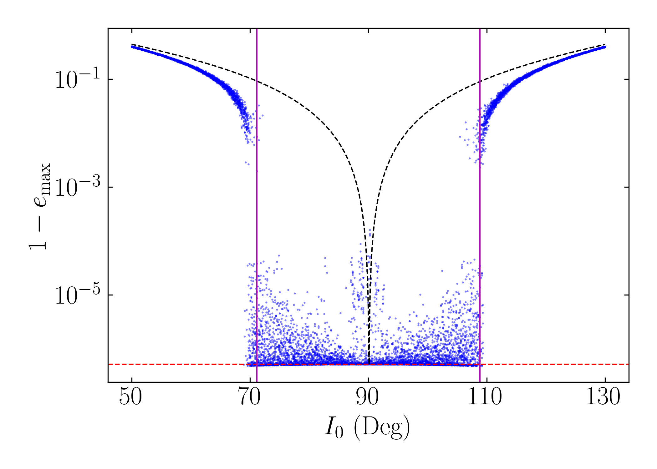
Figure 2: The maximum eccentricity achieved for an inner binary in the test-particle limit as a function of the initial inclination angle $I_{0}$. The triple system parameters are: $a=100\;\mathrm{AU}$, $a_{\rm out,eff}=3600\;\mathrm{AU}$, $m_{12}=50M_{\odot}$, $m_{3}=30M_{\odot}$, and $e_{\rm out}=0.6$; the corresponding octupole strength parameter is $\epsilon_{\rm oct}=0.02$ and $\eta\simeq 0$. The octupole-level secular equations of motion are integrated for $2000t_{\rm ZLK}$ (see Eq. 3), and the maximum eccentricity attained during this time is recorded and shown as a blue dot for each initial condition. We consider $1000$ initial inclinations in the range $50^{\circ}\leq I_{0}\leq 130^{\circ}$, and each $I_{0}$ is simulated five times, with the initial orbital elements $\omega$, $\omega_{\rm out}$, and $\Omega=\Omega_{\rm out}-\pi$ chosen randomly $\in[0,2\pi)$ for each simulation. The dotted black line shows the quadrupole-level result (Eq. 7 with $\eta=0$), and $e_{\lim}$ (Eq. 9) is shown as the horizontal red line. The vertical purple lines denote the boundary of the octupole-active inclination window, based on the fitting formula from Muñoz et al. (2016) (Eq. 12).

The relative strength of the octupole-order potential to the quadrupole-order potential is determined by the dimensionless parameter $\epsilon_{\rm oct}$ (Eq. 2). When $\epsilon_{\rm oct}$ is non-negligible, $K$ is no longer conserved, and the system evolution becomes chaotic (Ford et al., 2000; Katz et al., 2011; Lithwick & Naoz, 2011; Li et al., 2014; Liu et al., 2015). As a result, analytical (and semi-analytical) results have only been given for the test-particle limit, where $m_{2}=\eta=0$. We briefly review these results below.

Due to the non-conservation of $K$, $e_{\max}$ evolves irregularly ZLK cycles, and the orbit may even flip between prograde ($I<90^{\circ}$) and retrograde ($I>90^{\circ}$) if $K$ changes sign (in the test-particle limit, $K=j(e)\cos I$). During these orbit flips, the eccentricity maxima reach their largest values but do not exceed $e_{\lim}$ (Lithwick & Naoz, 2011; Liu et al., 2015; Anderson et al., 2016). These orbit flips occur on characteristic timescale $t_{\rm ZLK,oct}$, given by (Antognini, 2015)

$$t_{\rm ZLK,oct}=t_{\rm ZLK}\frac{128\sqrt{10}}{15\pi\sqrt{\epsilon_{\rm oct}}}.$$ (11)

The octupole potential tends to widen the inclination range for which the eccentricity can reach $e_{\lim}$; we refer to this widened range as the octupole-active window. Figure 2 shows the maximum eccentricity attained by an inner binary orbited by a tertiary companion with inclination $I_{0}$. The octupole-active window is visible as a range of inclinations centered on $I_{0}=90^{\circ}$ that attain $e_{\lim}$ (the red horizontal dashed line in Fig. 2). Katz et al. (2011) show that this window can be approximated using analytical arguments when $\epsilon_{\rm oct}\ll 1$. Muñoz et al. (2016) give a more general numerical fitting formula describing the octupole-active window for arbitrary $\epsilon_{\rm oct}$. They find that orbit flips and extreme eccentricity excitation occur for $I_{\rm flip,-}\lesssim I_{0}\lesssim I_{\rm flip,+}$ where

$$\cos^{2}I_{\rm flip,\pm}=\begin{cases}0.26\left(\frac{\epsilon_{\rm oct}}{0.1}\right)-0.536\left(\frac{\epsilon_{\rm oct}}{0.1}\right)^{2}\\ \quad+12.05\left(\frac{\epsilon_{\rm oct}}{0.1}\right)^{3}-16.78\left(\frac{\epsilon_{\rm oct}}{0.1}\right)^{4}&\epsilon_{\rm oct}\lesssim 0.05,\\ 0.45&\epsilon_{\rm oct}\gtrsim 0.05.\end{cases}$$ (12)

In Fig. 2, we see that with the octupole effect included, $e_{\max}$ indeed attains $e_{\lim}$ when $I_{0}$ is within the broad octupole-active window given by Eq. (12) (denoted by the vertical purple lines in Fig. 2).

2.3 Octupole Order: General Masses

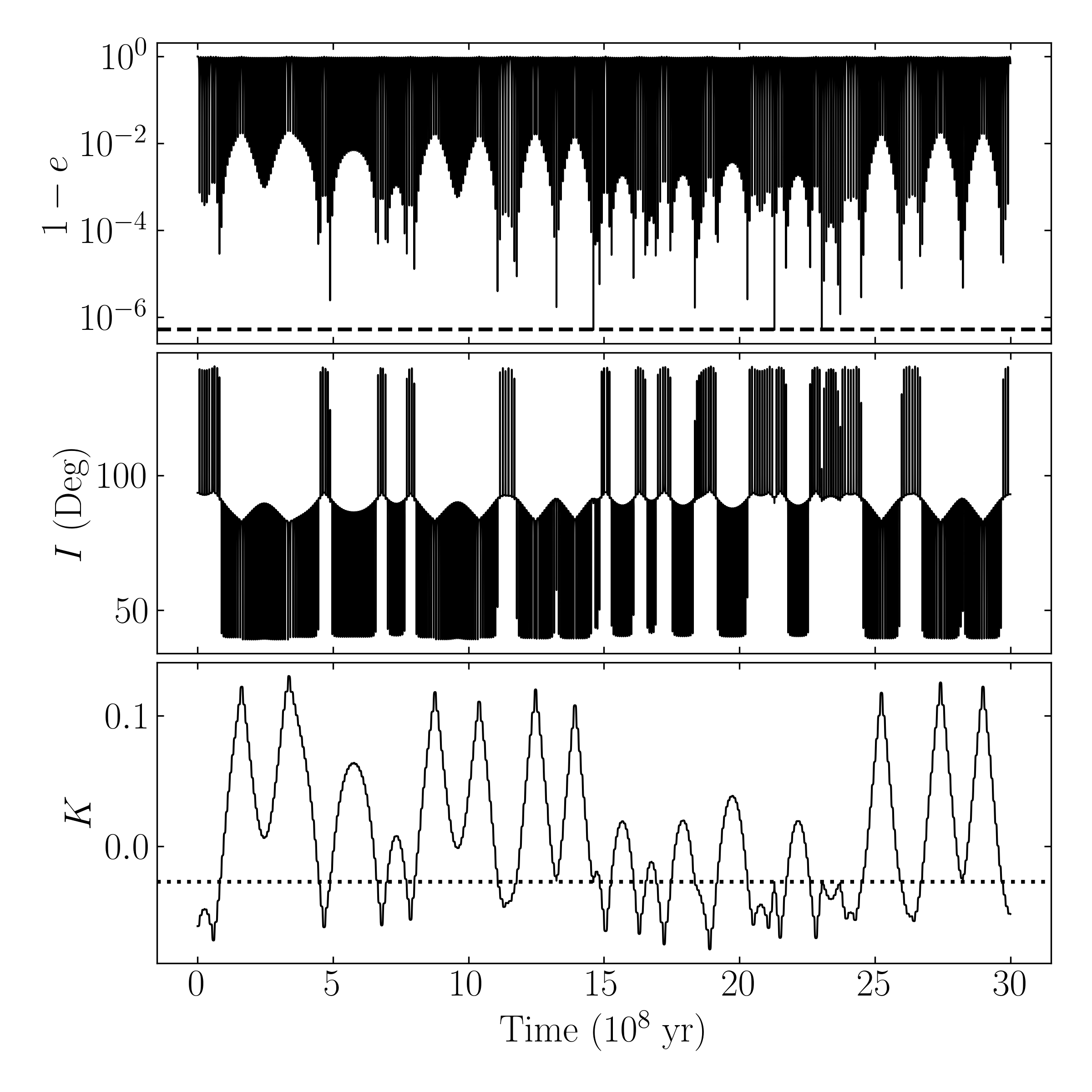
Figure 3: An example of the triple evolution for a system with significant octupole effects and finite $\eta$ (see Eq. 5). We use the same system parameters as in Fig. 2 except for $q=0.2$, corresponding to $\eta\approx 0.087$ and $\epsilon_{\rm oct}\approx 0.007$, and $I_{0}=93.5^{\circ}$. The three panels show the inner orbit eccentricity, the mutual inclination, and the generalized “Kozai constant” $K$ (Eq. 4). In the first panel, $e_{\lim}$ is denoted by the black dashed line. By comparing the second and third panels, we see that orbit flips occur when $K$ crosses the dotted line, given by $K=K_{\rm c}\equiv-\eta/2$.

For general inner binary masses, when the angular momentum ratio $\eta$ is non-negligible, the octupole-level ZLK behavior is less well-studied (see Liu et al., 2015). Figure 3 shows an example of the evolution of a triple system with significant $\eta$ and $\epsilon_{\rm oct}$. Many aspects of the evolution discussed in Section 2.2 are still observed: the ZLK eccentricity maxima and $K$ evolve over timescales $\gg t_{\rm ZLK}$; the eccentricity never exceeds $e_{\lim}$; when $K$ crosses $K_{\rm c}\equiv-\eta/2$, an orbit flip occurs (this follows by inspection of Eq. 4).

However, Eq. (12) no longer describes the octupole-active window as $\eta$ is non-negligible (see also Rodet et al., 2021). In the top panel of Fig. 4, the blue dots show the maximum achieved eccentricity of a system with the same parameters as Fig. 2 except with $q=0.5$ (so $\epsilon_{\rm oct}=0.007$ and $\eta=0.087$). Here, it can be seen that no prograde systems can attain $e_{\lim}$, and only a small range of retrograde inclinations $\geq I_{\rm 0,\lim}$ (see Eq. 8) are able to reach $e_{\lim}$. In fact, there is even a clear double valued feature around $I\approx 75^{\circ}$ in the top panel of Fig. 4 that is not present in Fig. 2. If $q$ is decreased to $0.3$ (Fig. 5) or further to $0.2$ (Fig. 6), $\epsilon_{\rm oct}$ increases while $\eta$ decreases. This permits a larger number of prograde systems to reach $e_{\lim}$, though a small range of inclinations near $I_{0}=90^{\circ}$ still do not reach $e_{\lim}$; we call this range of inclinations the “octupole-inactive gap”. On the other hand, if $q$ is held at $0.5$ as in Fig. 4 and $e_{\rm out}$ is increased to $0.9$ while holding $a_{\rm out,eff}=3600\;\mathrm{AU}$ constant, both $\epsilon_{\rm oct}$ and $\eta$ increase; the top panel of Fig. 7 shows that prograde systems still fail to reach $e_{\lim}$ for these parameters, despite the increase in $\epsilon_{\rm oct}$. The top panel of Fig. 8 illustrates the behavior when the inner binary is substantially more compact ($a=10\;\mathrm{AU}$): even though $\epsilon_{\rm oct}$ is larger than it is in any of Figs. 4–7, we see that prograde perturbers fail to attain $e_{\lim}$. All of these examples (top panels of Figs. 4–8) illustrate importance of $\eta$ in determining the range of inclinations for the system to be able to reach $e_{\lim}$.

In general, we find that a symmetric octupole-active window (as in Eq. 12) can be realized for sufficiently small $\eta$. Rodet et al. (2021) considered some examples of triple systems (consisting of MS stars with planetary companions and tertiaries, for which the short-range forces is dominated by tidal interaction) and found that $\eta\lesssim 0.1$ is sufficient for a symmetric octupole-active window. In the cases considered in this paper, a smaller $\eta$ is necessary (e.g., $\eta\simeq 0.054$ in Fig. 6). Thus, the critical $\eta$ above which the symmetry of the octupole-active window is significantly broken likely depends on the dominant short-range forces and $e_{\lim}$ [in Rodet et al. (2021), $1-e_{\lim}\sim 10^{-3}$, while in Figs. 2 and 4–8, $1-e_{\lim}\lesssim 10^{-5}$]. In general, when $\eta$ is non-negligible, there are up to two octupole-active windows: a prograde window whose existence depends on the specific values of $\eta$ and $\epsilon_{\rm oct}$, and a retrograde window that always exists.

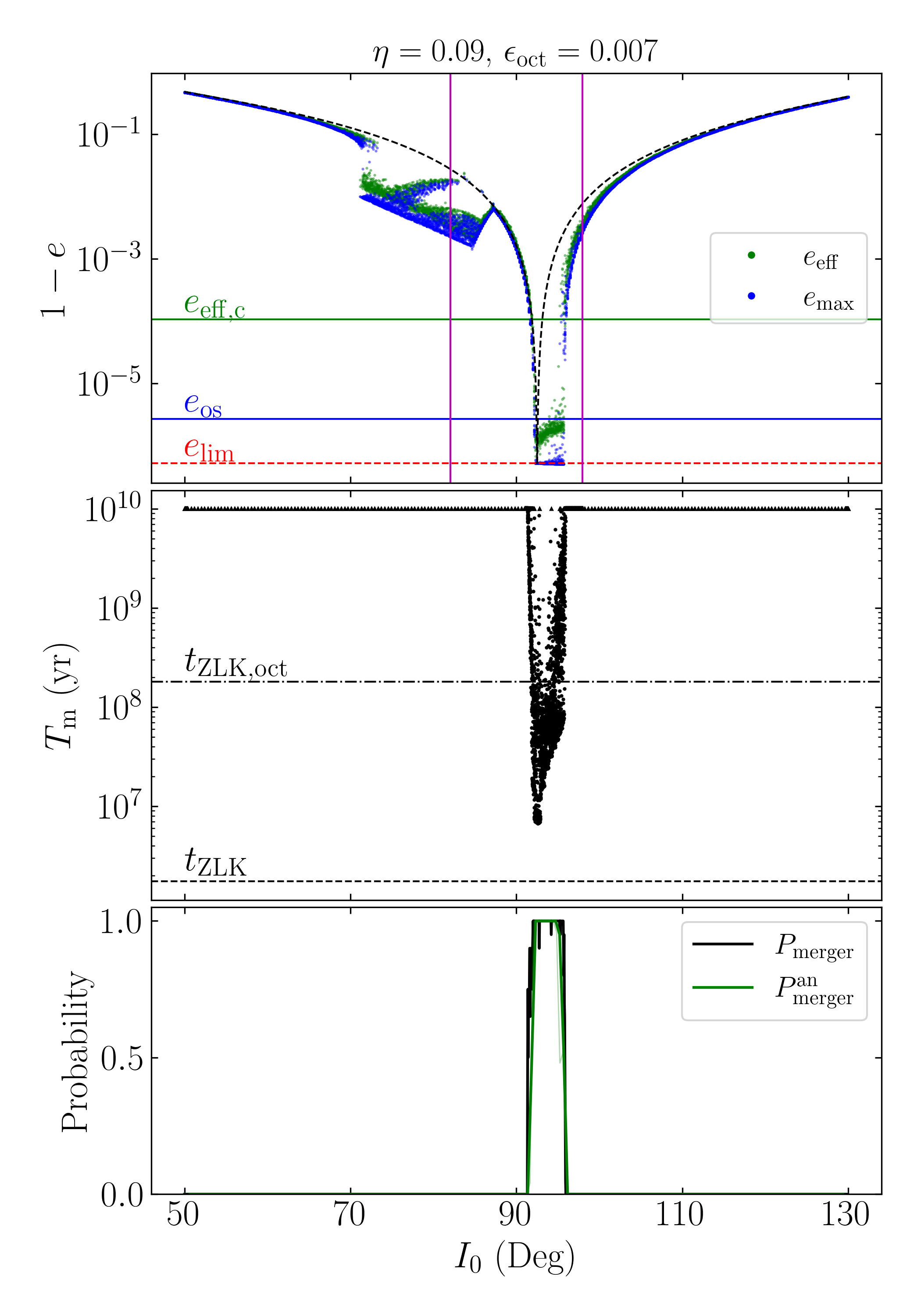
Figure 4: Eccentricity excitation and merger windows for the fiducial BH triple system ($a=100\;\mathrm{AU}$, $a_{\rm out,eff}=3600\;\mathrm{AU}$, $m_{12}=50M_{\odot}$, $m_{3}=30M_{\odot}$) with $q=0.5$ and $e_{\rm out}=0.6$, corresponding to $\eta\approx 0.087$ and $\epsilon_{\rm oct}\approx 0.007$. In the top panel, for each of $1000$ initial inclinations, we choose $5$ different random $\omega$, $\omega_{\rm out}$, and $\Omega$ as initial conditions and evolve the system for $2000t_{\rm ZLK}$ without GW radiation. The effective eccentricity $e_{\rm eff}$ (Eq. 21; green dots) as well as the maximum eccentricity $e_{\max}$ (blue dots) over this period are displayed. For comparison, $e_{\rm eff,c}$ (Eq. 22) is given by the horizontal green dashed line, $e_{\rm os}$ (Eq. 18) is shown as the horizontal blue line, and $e_{\lim}$ (Eq. 9) is shown as the horizontal red dashed line. The vertical purple lines denote the test-mass octupole-active window and are given by the fitting formula of Muñoz et al. (2016); they do not longer accurately describe the $e_{\lim}$-attaining inclination window because $\eta$ is finite. The black dashed line is is the quadrupole-level result as given by Eq. (7). In the middle panel, we show the binary merger times when including GW radiation and using the same range of initial conditions. Numerical integrations are terminated when $T_{\rm m}>10\;\mathrm{Gyr}$ and marked as unsuccessful mergers. The horizontal dashed line denotes $t_{\rm ZLK}$ (Eq. 3) while the horizontal dash-dotted line indicates $t_{\rm ZLK,oct}$ (Eq. 11). Here, each $I_{\rm 0}$ is run $20$ times with uniform distributions of $\omega$, $\omega_{\rm out}$, and $\Omega$, so we can estimate the merger probability $P_{\rm merger}$ (Eq. 16) for each $I_{\rm 0}$ – $P_{\rm merger}$ is shown as the black line in the bottom panel. As described in Section 3.2, the merger probability can be predicted semi-analytically using the results of the top panel and Eq. (24), and is denoted by $P_{\rm merger}^{\rm an}$. In the bottom panel, the thick green line shows $P_{\rm merger}^{\rm an}$ when using an integration time of $2000t_{\rm ZLK}\approx 3\;\mathrm{Gyr}$ for the non-dissipative simulations, and thin green line shows the prediction using an integration time of $500t_{\rm ZLK}$. The agreement of $P_{\rm merger}^{\rm an}$ with $P_{\rm merger}$ is good and improves when using the longer integration time.

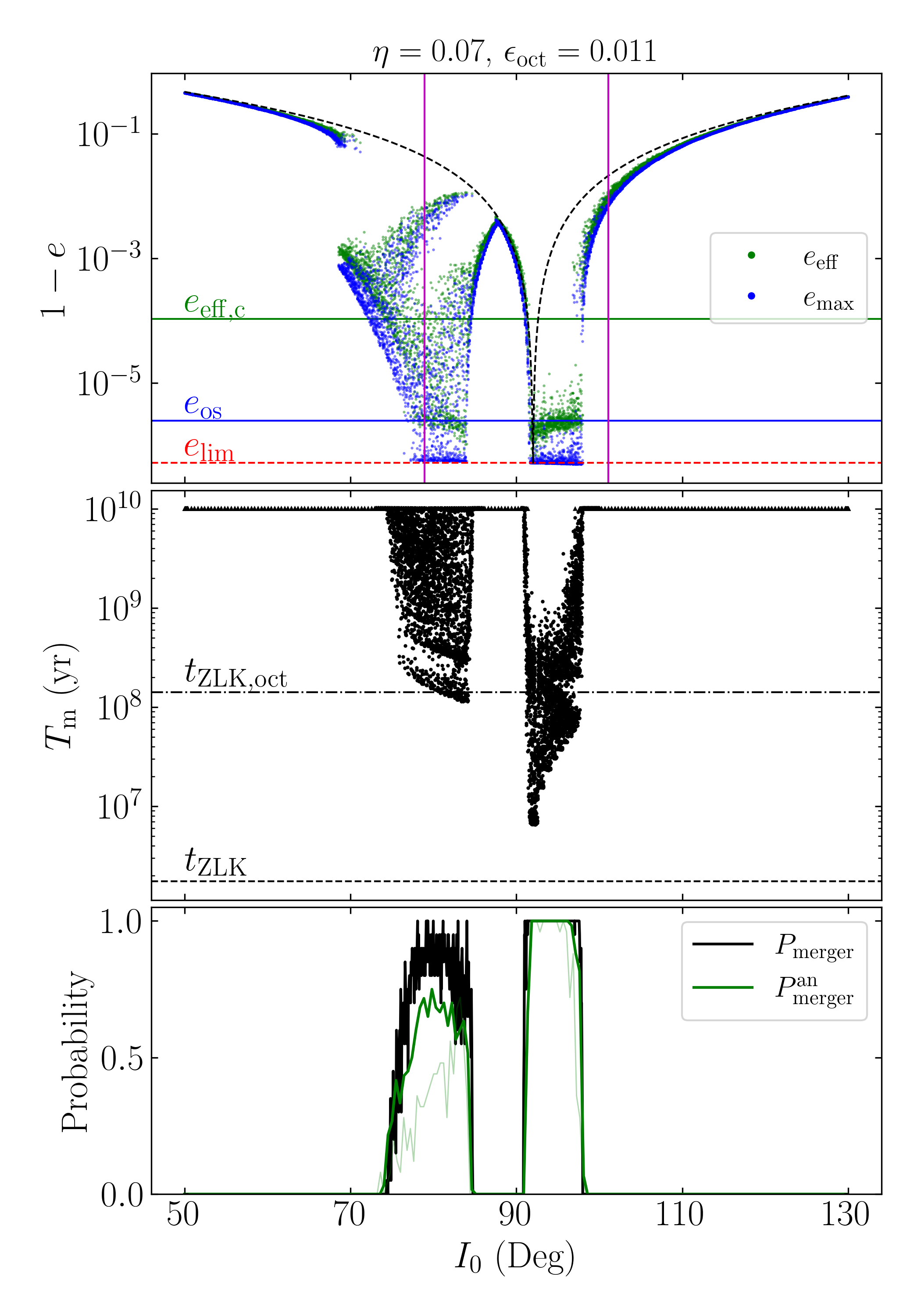
Figure 5: Same as Fig. 4 but for $q=0.3$, corresponding to $\eta\approx 0.07$ and $\epsilon_{\rm oct}\approx 0.011$.

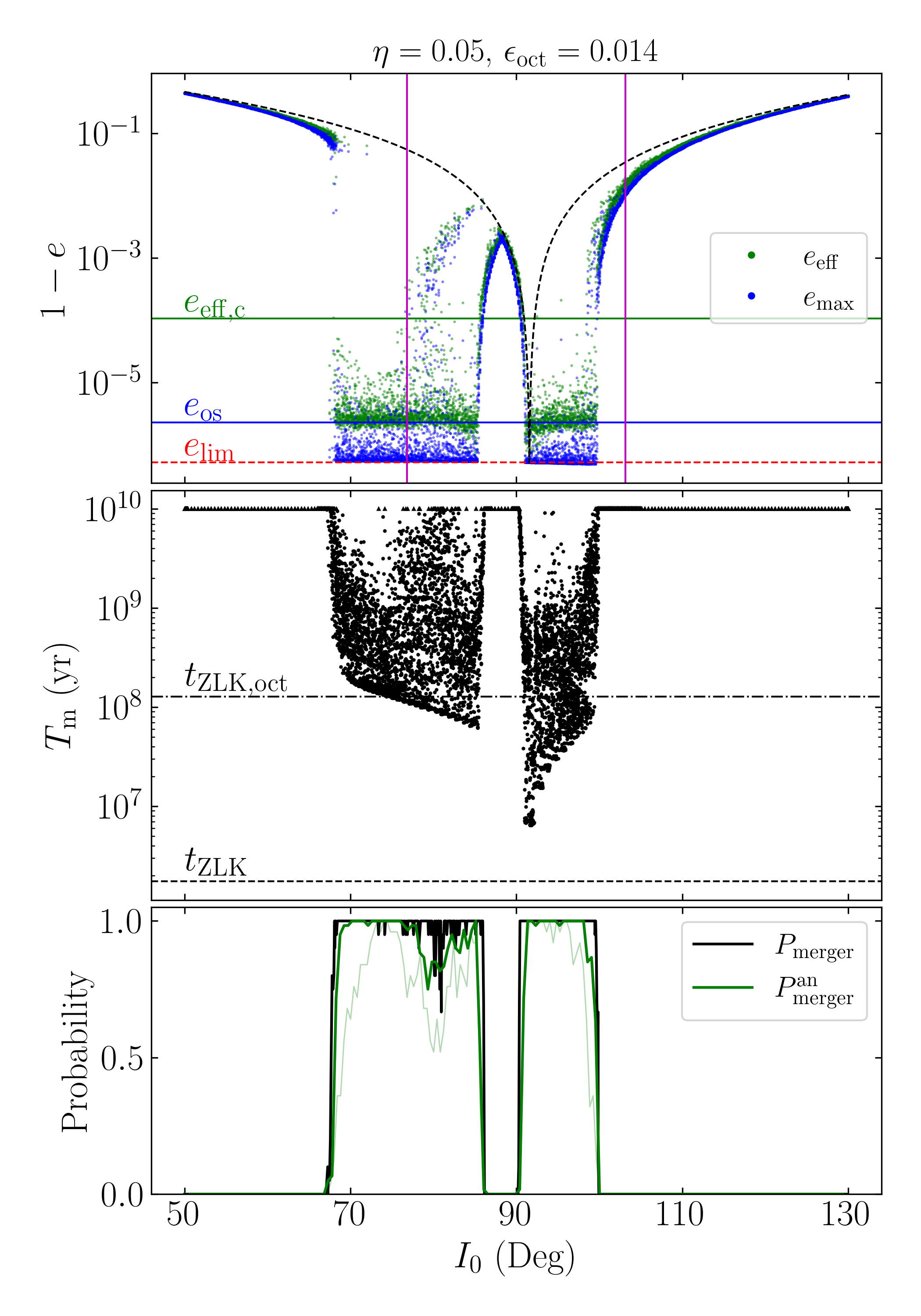
Figure 6: Same as Fig. 4 but for $q=0.2$, corresponding to $\eta\approx 0.054$ and $\epsilon_{\rm oct}\approx 0.014$.

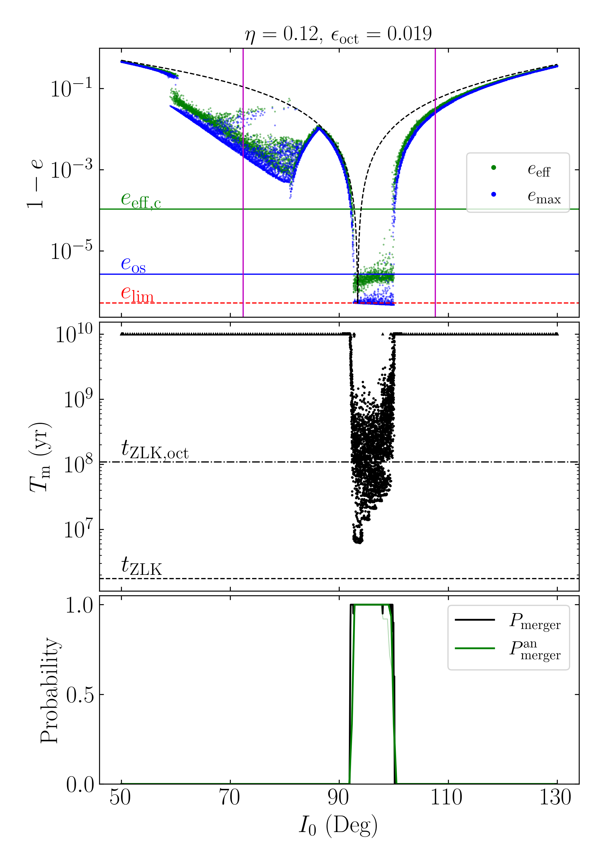
Figure 7: Same as Fig. 4 but for $e_{\rm out}=0.9$ while holding $a_{\rm out,eff}$ the same, corresponding to $\eta=0.118$ and $\epsilon_{\rm oct}=0.019$.

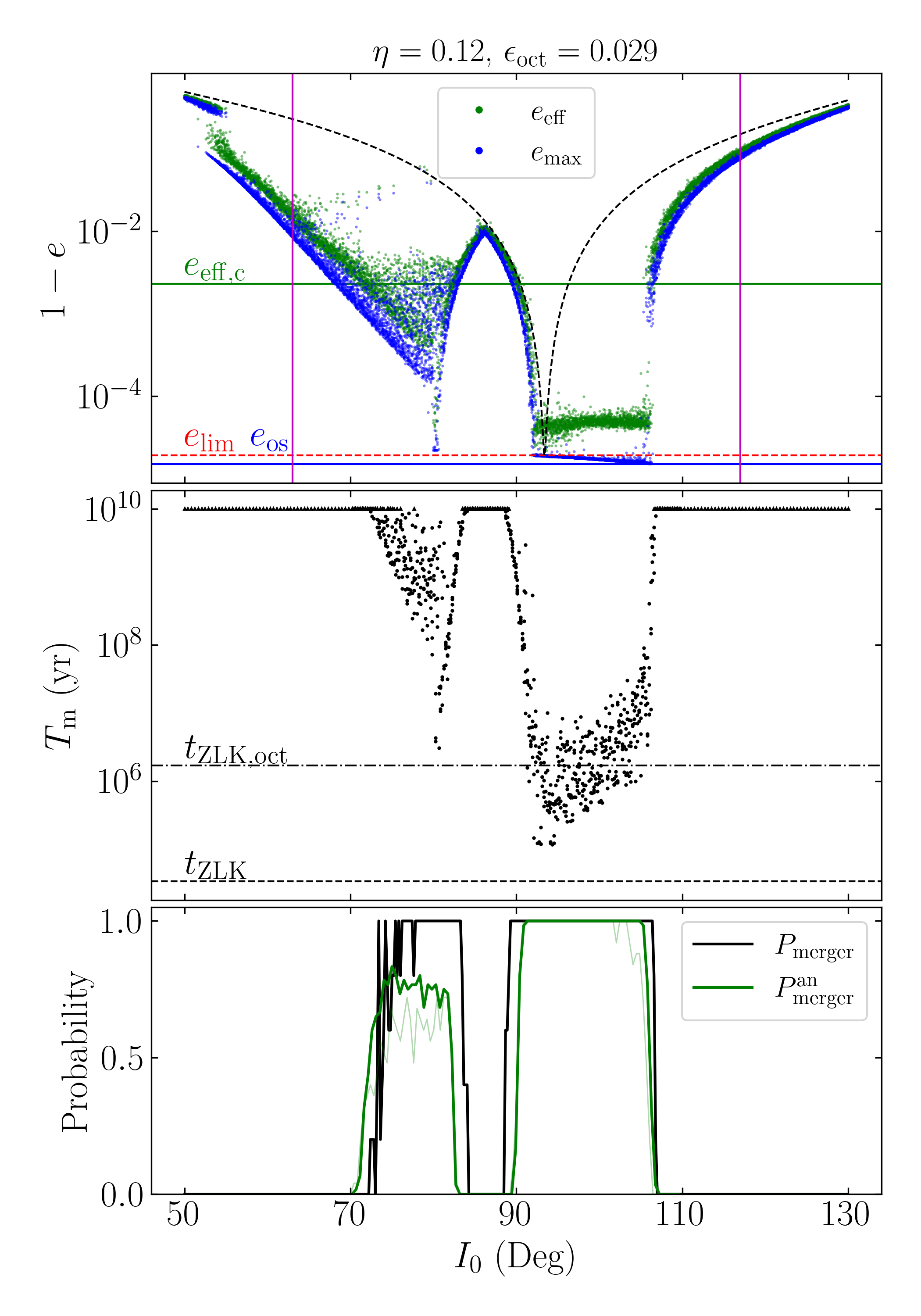
Figure 8: Same as Fig. 4 but for a more compact inner binary; the parameters are $a_{0}=10\;\mathrm{AU}$, $a_{\rm out,eff}=700\;\mathrm{AU}$, $m_{12}=50M_{\odot}$, $m_{3}=30M_{\odot}$, $e_{\rm out}=0.9$, and $q=0.4$, corresponding to $\eta=0.118$ and $\epsilon_{\rm oct}=0.029$. Here, $P_{\rm merger}$ is computed with only $5$ integrations (for random $\omega$, $\omega_{\rm out}$, and $\Omega$) for each $I_{0}$.

3 Tertiary-Induced Black Hole Mergers

Emission of gravitational waves (GWs) affects the evolution of the inner binary, which can be incorporated into the secular equations of motion for the triple (e.g., Peters, 1964; Liu & Lai, 2018). The associated orbital and eccentricity decay rates are (Peters, 1964):

$$\left.\frac{1}{a}\frac{\mathrm{d}a}{\mathrm{d}t}\right|_{\rm GW} \equiv-\frac{1}{t_{\rm GW}}$$

$$=-\frac{64}{5}\frac{G^{3}\mu m_{12}^{2}}{c^{5}a^{4}j^{7}(e)}\left(1+\frac{73}{24}e^{2}+\frac{37}{96}e^{4}\right),$$ (13)

$$\left.\frac{\mathrm{d}e}{\mathrm{d}t}\right|_{\rm GW} =-\frac{304}{15}\frac{G^{3}\mu m_{12}^{2}}{c^{5}a^{4}}\frac{1}{j^{5}(e)}\left(1+\frac{121}{304}e^{2}\right).$$ (14)

GW emission can cause the orbit to decay significantly when extreme eccentricities are reached during the ZLK cycles described in the previous section. This allows even wide binaries ($\sim 100\;\mathrm{AU}$) to merge efficiently within a Hubble time. While various numerical examples of such tertiary-induced mergers have been given before (e.g., Liu & Lai (2018); see also Liu et al. (2019a) for “population synthesis”), in this section we examine the dynamical process in detail in order to develop an analytical understanding. Our fiducial system parameters are as in Fig. 3: $a_{\rm out,eff}=4500\;\mathrm{AU}$, $e_{\rm out}=0.6$, $m_{12}=50M_{\odot}$ (with varying $q$), $m_{3}=30M_{\odot}$, and the inner binary has initial $a_{0}=100\;\mathrm{AU}$ and $e_{0}=10^{-3}$.

3.1 Merger Windows and Probability: Numerical Results

To understand what initial conditions lead to successful mergers within a Hubble time, we integrate the double-averaged octupole-order ZLK equations including GW radiation. We terminate each integration if either $a=0.005a_{0}$ (a successful merger) or the system age reaches $10\;\mathrm{Gyr}$. We can verify that the inner binary is effectively decoupled from the tertiary for this orbital separation by evaluating $\epsilon_{\rm GR}$ (Eq. 6):

$$\epsilon_{\rm GR}=1.8\times 10^{6}\left(\frac{m_{12}}{50M_{\odot}}\right)^{2}\left(\frac{a_{\rm out,eff}}{3600\;\mathrm{AU}}\right)^{3}\left(\frac{m_{3}}{30M_{\odot}}\right)^{-1}\left(\frac{a}{0.5\;\mathrm{AU}}\right)^{-4}.$$ (15)

The middle panel of Fig. 4 shows the merger time $T_{\rm m}$ as a function of $I_{0}$ for our fiducial parameters with $q=0.5$. We note that only retrograde inclinations lead to successful mergers, and almost all successful mergers are rapid, with $T_{\rm m}\sim t_{\rm ZLK,oct}$. These are the result of a system merging by emitting a single large burst of GW radiation during an extreme-eccentricity ZLK cycle, which we term a “one-shot merger”. In Fig. 5, $q$ is decreased to $0.3$, and some prograde systems are also able to merge successfully. However, these prograde systems exhibit a broad range of merger times, with $T_{\rm m}\gtrsim t_{\rm ZLK,oct}$. These occur when a system gradually emits a small amount of GW radiation at every eccentricity maximum – we term this a “smooth merger”. Additionally, the octupole-inactive gap near $I_{0}=90^{\circ}$ is visible in the merger time plot (middle panel of Fig. 5). The middle panels of Figs. 6–8 show the behavior of $T_{\rm m}$ for the other parameter regimes and also exhibit these two categories of mergers and the octupole-inactive gap.

Due to the chaotic nature of the octupole-order ZLK effect, the initial inclination $I_{0}$ alone is not sufficient to determine with certainty whether a system can merge within a Hubble time. Instead, for a given $I_{0}$, we can use numerical integrations with various $\omega$, $\omega_{\rm out}$, and $\Omega$ to compute a merger probability, denoted by

$$P_{\rm merger}\left(I_{0};q,e_{\rm out}\right)=P\left(T_{\rm m}<10\;\mathrm{Gyr}\right),$$ (16)

where the notation $P_{\rm merger}\left(I_{0};q,e_{\rm out}\right)$ highlights the dependence of $P_{\rm merger}$ on $q$ and $e_{\rm out}$, two of the key factors that determine the strength of the octupole effect (of course $P_{\rm merger}$ depends on other system parameters such as $m_{12}$, $a_{0}$, $a_{\rm out}$, etc.). The bottom panels of Figs. 4–8 show our numerical results. In all of these plots, there is a retrograde inclination window for which successful merger is guaranteed. In Fig. 5, it can be seen that a large range of prograde inclinations have a probabilistic outcome. In Fig. 6, while the enhanced octupole strength allows for most of the prograde inclinations to merge with certainty, there is still a region around $I_{0}\approx 80^{\circ}$ where $P_{\rm merger}<1$.

3.2 Merger Probability: Semi-analytic Criteria

By comparing the top and bottom panels of Figs. 4–8, it is clear that their features are correlated: in all five cases, the retrograde merger window occupies the same inclination range as the retrograde octupole-active window, while $P_{\rm merger}$ is only nonzero for prograde inclinations where $e_{\max}$ nearly attains $e_{\lim}$. Here, we further develop this connection and show that the non-dissipative simulations can be used to predict the outcomes of simulations with GW dissipation rather reliably.

In Section 3.1, we identified both one-shot and smooth mergers in our simulations. Towards understanding the one-shot mergers, we first define $e_{\rm os}$ to be the $e_{\max}$ required to dissipate an order-unity fraction of the binary’s orbital energy via GW emission in a single ZLK cycle. Since a binary spends a fraction $\sim j(e_{\max})$ of each ZLK cycle near $e_{\max}$ (e.g., Anderson et al., 2016), we set

$$j\left(e_{\rm os}\right)\left.\frac{\mathrm{d}\ln a}{\mathrm{d}t}\right|_{e=e_{\rm os}}=-\frac{1}{t_{\rm ZLK}},$$ (17)

where $\mathrm{d}(\ln a)/\mathrm{d}t$ is given by Eq. (13). This yields

$$j^{6}(e_{\rm os})\equiv\frac{425t_{\rm ZLK}}{96t_{\rm GW,0}}=\frac{170}{3}\frac{G^{3}\mu m_{12}^{3}}{m_{3}c^{5}a^{4}n}\left(\frac{a_{\rm out,eff}}{a}\right)^{3},$$ (18)

where $t_{\rm GW,0}=(t_{\rm GW})_{e=0}$ (see Eq. 13) is given by

$$t_{\rm GW,0}^{-1}=\frac{64}{5}\frac{G^{3}\mu m_{12}^{2}}{c^{5}a^{4}},$$ (19)

we have approximated $e_{\rm os}\approx 1$. Eq. (18) is equivalent to

$$1-e_{\rm os}\approx{} 3\times 10^{-6}\left(\frac{m_{12}}{50M_{\odot}}\right)^{7/6}\left(\frac{q/(1+q)^{2}}{1/4}\right)^{1/3}\left(\frac{m_{3}}{30M_{\odot}}\right)^{-1/3}$$

$$\times\left(\frac{a_{\rm out,eff}}{3600\;\mathrm{AU}}\right)\left(\frac{a}{100\;\mathrm{AU}}\right)^{-11/6}.$$ (20)

Then, if a system satisfies $e_{\max}>e_{\rm os}$ with $e_{\max}$ based on non-dissipative integration, it is expected attain a sufficiently large eccentricity to undergo a one-shot merger.

Towards understanding smooth mergers, we seek a characteristic eccentricity that captures GW emission over many ZLK cycles. We define $e_{\rm eff}$ as an effective ZLK maximum eccentricity, i.e.

$$\left\langle\frac{\mathrm{d}\ln a}{\mathrm{d}t}\right\rangle =-\frac{1}{t_{\rm GW,0}}\left\langle\frac{1+73e^{2}/24+37e^{4}/96}{j^{7}(e)}\right\rangle$$

$$\equiv-\frac{425/96}{t_{\rm GW,0}}\frac{1}{j^{6}(e_{\rm eff})},$$ (21)

where the angle brackets denote averaging over many $t_{\rm ZLK,oct}$ in order to capture the characteristic eccentricity behavior over many octupole cycles. In the second line of Eq. (21), we have essentially replaced the ZLK-averaged orbital decay rate by $\mathrm{d}(\ln a)/\mathrm{d}t$ evaluated at $e_{\rm eff}$ multiplied by $j(e_{\rm eff})$. In practice (see Figs. 4–8), we typically average over $2000t_{\rm ZLK}$ of the non-dissipative simulations to compute $e_{\rm eff}$.

With $e_{\rm eff}$ computed using Eq. (21), we can define the critical effective eccentricity $e_{\rm eff,c}$ such that the ZLK-averaged inspiral time is a Hubble time, i.e. $\left\langle\mathrm{d}(\ln a)/\mathrm{d}t\right\rangle\equiv-\left(10\;\mathrm{Gyr}\right)^{-1}$. This gives

$$j^{6}\left(e_{\rm eff,c}\right)\equiv\frac{425}{96}\frac{10\;\mathrm{Gyr}}{t_{\rm GW,0}},$$ (22)

or equivalently

$$1-e_{\rm eff,c}\approx 10^{-4}\left(\frac{m_{12}}{50M_{\odot}}\right)\left(\frac{q/(1+q)^{2}}{1/4}\right)^{1/3}\left(\frac{a}{100\;\mathrm{AU}}\right)^{-4/3}.$$ (23)

Thus, if a system is evolved using the non-dissipative equations of motion and satisfies $e_{\rm eff}>e_{\rm eff,c}$, then it is expected to successfully undergo a smooth merger within a Hubble time.

Therefore, a system can be predicted to merge successfully if it satisfies either the one-shot or smooth merger criteria. The semi-analytical merger probability (as a function of $I_{0}$ and other parameters) is:

$$P_{\rm merger}^{\rm an}\left(I_{0};q,e_{\rm out}\right)=P\left(e_{\rm eff}>e_{\rm eff,c}\;\;\text{or}\;\;e_{\max}>e_{\rm os}\right).$$ (24)

Although not fully analytical (since numerical integrations of non-dissipative systems are needed to obtain $e_{\rm eff}$ and $e_{\max}$ in general), Eq. (24) provides efficient computation of the merger probability without full numerical integrations including GW radiation.

The top panels of Figs. 4–8 show $e_{\rm eff}$ and $e_{\max}$, and their critical values, $e_{\rm eff,c}$ and $e_{\rm os}$. Using these, we compute the semi-analytical merger probability, shown as the thick green lines in the bottom panels of Figs. 4–8. We generally observe good agreement with the numerical $P_{\rm merger}$. However, $P_{\rm merger}^{\rm an}$ slightly but systematically underpredicts $P_{\rm merger}$ for some configurations, such as the prograde inclinations in Figs. 5 and 8. These regions coincide with the inclinations for which the merger outcome is uncertain. This underprediction is due to the restricted integration time of $2000t_{\rm ZLK}\approx 3\;\mathrm{Gyr}$ used for the non-dissipative simulations. To illustrate this, we also calculate $P_{\rm merger}^{\rm an}$ using a shorter integration time of $500t_{\rm ZLK}$ for our non-dissipative simulations. The results are shown as the light green lines in the bottom panels of Figs. 4–8, performing visibly worse. A more detailed discussion of this issue can be found in Section 4.4.

A few observations about Eq. (24) can be made. First, it explains why some prograde systems merge probabilistically ($0<P_{\rm merger}<1$): for the prograde inclinations in Fig. 5, the $e_{\rm eff}$ values scatter widely around $e_{\rm eff,c}$ [or more precisely, $j(e_{\rm eff})$ scatters around $j(e_{\rm eff,c})$], even for a given $I_{0}$, so the detailed merger outcome depends on the initial conditions. For the prograde inclinations in Fig. 6, the double-valued feature in the $e_{\max}$ plot (the top panel) pointed out in Section 2.3 represents a sub-population of systems that do not satisfy Eq. (24). Second, $e_{\max}>e_{\rm os}$ often ensures $e_{\rm eff}>e_{\rm eff,c}$ in practice, as the averaging in Eq. (21) is heavily weighted towards extreme eccentricities. As such, $e_{\rm eff}>e_{\rm eff,c}$ alone is often a sufficient condition in Eq. (24).

The one-shot merger criterion ($e_{\max}>e_{\rm os}$) can also be used to distinguish two different types of system architectures: if $e_{\lim}\gtrsim e_{\rm os}$ for a particular architecture, then all initial conditions leading to orbit flips (i.e., in an octupole-active window) also execute one-shot mergers. For $e_{\lim}\approx 1$, Eq. (9) reduces to

$$j(e_{\lim})\approx\frac{8\epsilon_{\rm GR}}{9}\left(1+\frac{\eta^{2}}{12}\right)^{-1}.$$ (25)

which lets us rewrite the constraint $e_{\lim}\gtrsim e_{\rm os}$ as

$$\left(\frac{a}{a_{\rm out,eff}}\right)\gtrsim{} 0.0186\left(\frac{a_{\rm out,eff}}{3600\;\mathrm{AU}}\right)^{-7/37}\left(\frac{m_{12}}{50M_{\odot}}\right)^{17/37}$$

$$\times\left(\frac{30M_{\odot}}{m_{3}}\right)^{10/37}\left(\frac{q/(1+q)^{2}}{1/4}\right)^{-2/37}.$$ (26)

For the system architecture considered in Figs. 4–7, this condition is satisfied, and we see indeed that wherever the top panel suggests orbit flipping ($e_{\max}=e_{\lim}$), the bottom panel shows $P_{\rm merger}\approx 1$. When the condition (Eq. 26) is not satisfied, one-shot mergers are not possible, and $P_{\rm merger}$ is generally only nonzero for a small range about $I_{\rm 0,\lim}$.

4 Merger Fraction as a Function of Mass Ratio

Having developed an semi-analytical understanding of the binary merger window and probability in the last section (particularly Section 3.2), we now study the fraction of BH binaries in triples that successfully merge under various conditions – we call this the merger fraction.

4.1 Merger Fraction for Fixed Tertiary Eccentricity

We first consider the simple case where $e_{\rm out}$ is fixed at a few specific values and compute the merger fraction as a function of the mass ratio $q$. We consider isotropic mutual orientations between the inner and outer binaries, i.e. we draw $\cos I_{0}$ from a uniform grid over the range $[-1,1]$ (recall that $\omega$, $\omega_{\rm out}$, and $\Omega$ are drawn uniformly from the range $[0,2\pi)$ when computing the merger probability $P_{\rm merger}$ at a given $I_{0}$). The merger fraction is then given by:

$$f_{\rm merger}\left(q,e_{\rm out}\right)\equiv\frac{1}{2}\int\limits_{-1}^{1}\mathrm{d}\cos I_{0}\;P_{\rm merger}\left(I_{0};q,e_{\rm out}\right).$$ (27)

This is proportional to the integral of the black lines (weighted by $\sin I_{0}$) in the bottom panels of Figs. 4–7. We can also use semi-analytical criteria introduced in Section 3.2 to predict the outcome and merger fraction. This is computed by using $P_{\rm merger}^{\rm an}$ as the integrand in Eq. (27), or by evaluating the integral of the thick green lines (weighted by $\sin I_{0}$) in the bottom panels of Figs. 4–7. Figure 9 shows the resulting $f_{\rm merger}$ and the analytical estimates for all combinations of $q\in\left\{0.2,0.3,0.4,0.5,0.7,1.0\right\}$ and $e_{\rm out}\in\left\{0.6,0.8,0.9\right\}$. It is clear that the numerical $f_{\rm merger}$ and the analytical estimate agree well, and that the merger fraction increases steeply for smaller $q$.

To explore the impact of our choice of isotropic mutual orientations between the two binaries, we also consider a wedge-shaped distribution of $\cos I_{0}$ as was found in the population synthesis studies of Antonini et al. (2017). We still use the same uniform grid of $\cos I_{0}$ as before, but weight each eccentricity by its probability probability density following the distribution:

$$P\left(\cos I_{0}\right)=\frac{1}{4}+\frac{\left|\cos I_{0}\right|}{2}.$$ (28)

The resulting $f_{\rm merger}$ for a tertiary with $\cos I_{0}$ distributed like Eq. (28) is shown as the dashed lines in Fig. 9. While the total merger fractions decrease, the strong enhancement of the merger fraction at smaller $q$ is unaffected.

In the right panel of Fig. 9, we see that the merger fractions for the three $e_{\rm out}$ values overlap for small $\epsilon_{\rm oct}$. This implies that $f_{\rm merger}$ depends only on $\epsilon_{\rm oct}$ in this regime, and not on the values of $q$ and $e_{\rm out}$ independently. From Fig. 4 (which has $\epsilon_{\rm oct}=0.007$), we see that this suggests that the size of the retrograde merger window only depends on $\epsilon_{\rm oct}$, much like what Eq. (12) shows for the test-particle limit. However, once $\epsilon_{\rm oct}$ is increased sufficiently, the three curves in the right panel of Fig. 9 cease to overlap. This can be attributed to their different $\eta$ values: for sufficiently small $\epsilon_{\rm oct}$, no prograde initial inclinations successfully merge (e.g., Fig. 4), and the merger fraction is solely determined by the size of the retrograde octupole-active window. But once $\epsilon_{\rm oct}$ is sufficiently large, prograde mergers become possible, and the merger fraction is also affected by the size of the octupole-inactive gap, which depends on $\eta$. This again illustrates the importance of the octupole-inactive gap, which we comment on in Appendix A.

Figure 10 depicts the merger fractions for systems with $a_{0}=50\;\mathrm{AU}$ (the other parameters are the same as in Fig. 9). According to Eq. (26), these systems no longer satisfy $e_{\lim}\gtrsim e_{\rm os}$, so the merger fraction is expected to diminish strongly and vary much more weakly with $q$, as one-shot mergers are no longer possible. This is indeed observed, particularly for the $e_{\rm out}=0.6$ curve in Fig. 10. We also remark that the semi-analytical prediction accuracy is poorer in this case than in Fig. 9. This is because the only mergers in this regime are smooth mergers. As can be seen for the prograde $I_{0}$ in Figs. 5 and 8, smooth mergers occur over a wide range of merger times $T_{\rm m}$, and the specific $T_{\rm m}$ that a system experiences depends sensitively on its chaotic evolution. Thus, Eq. (21) is a rather approximate estimate of the amount of GW emission that a real system emits during a smooth merger; indeed, the prograde regions of Figs. 5 and 8 show that the merger times for smooth mergers are systematically underpredicted by the semi-analytic merger criterion (see discussion in Section 4.4). The non-monotonicity of the semi-analytic merger fraction for $e_{\rm out}=0.6$ from $q=0.2$ to $q=0.3$ is due to small sample sizes and finite grid spacing in $\cos I_{0}$.

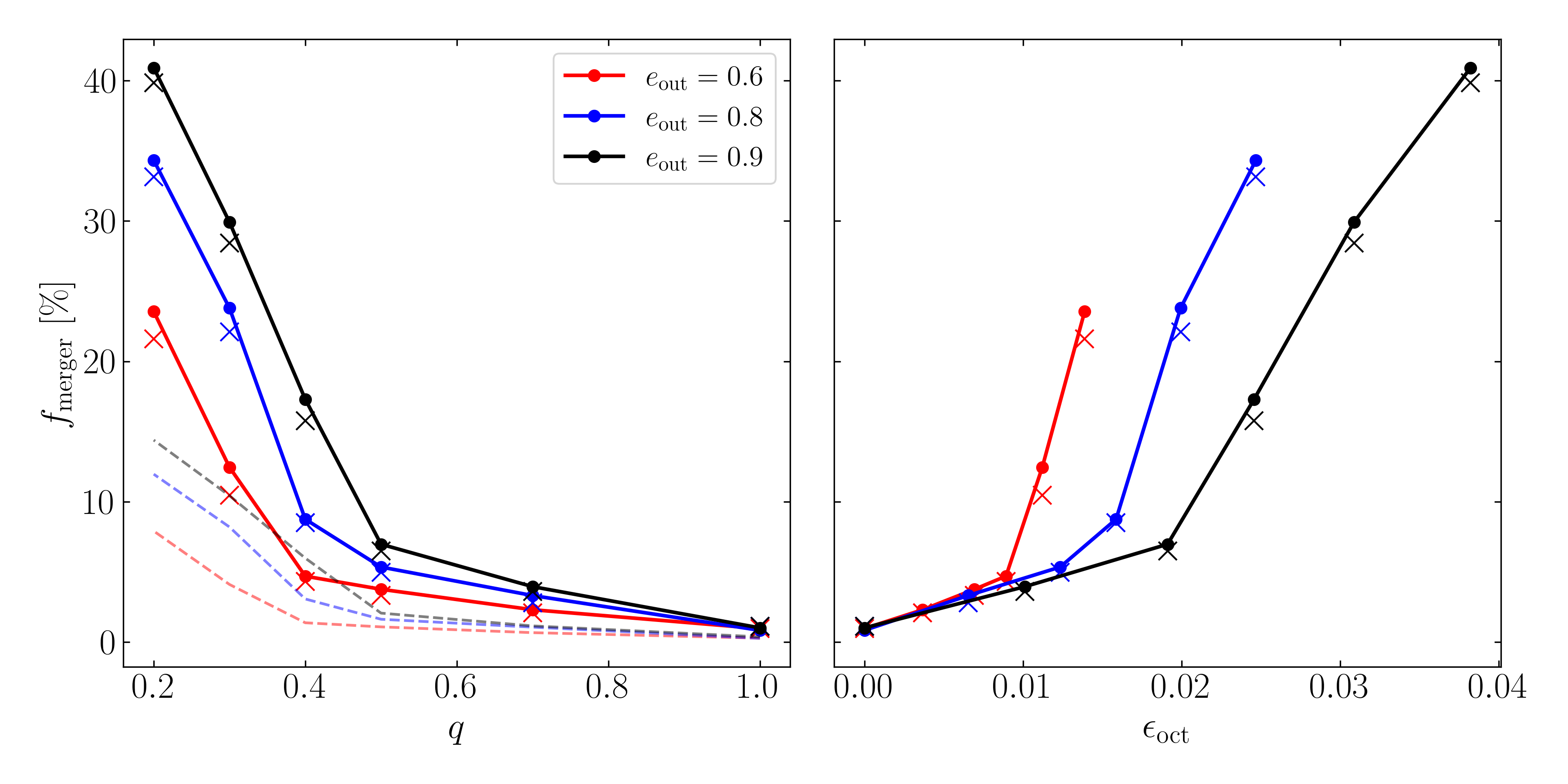
Figure 9: Merger fraction (Eq. 16) of BH binaries in triples as a function of mass ratio $q$ (left panel) for several values of outer binary eccentricities. The other system parameters are the same as in Figs. 4–7. The right panel shows the same merger fraction, but plotted against the octupole parameter $\epsilon_{\rm oct}$. The filled circles joined by the solid lines are numerical results (based on integrations for full triple system evolution including GW emission; see the black solid lines in the bottom panels of Figs. 4–7) assuming random mutual inclinations between the inner and outer binaries (uniform in $\cos I_{0}$), and the dashed lines denote the merger fractions if the mutual inclinations are distributed according to Eq. (28). The crosses are semi-analytical results using an integration time of $2000t_{\rm ZLK}$ (see the thick green lines in the bottom panels of Figs. 4–7).

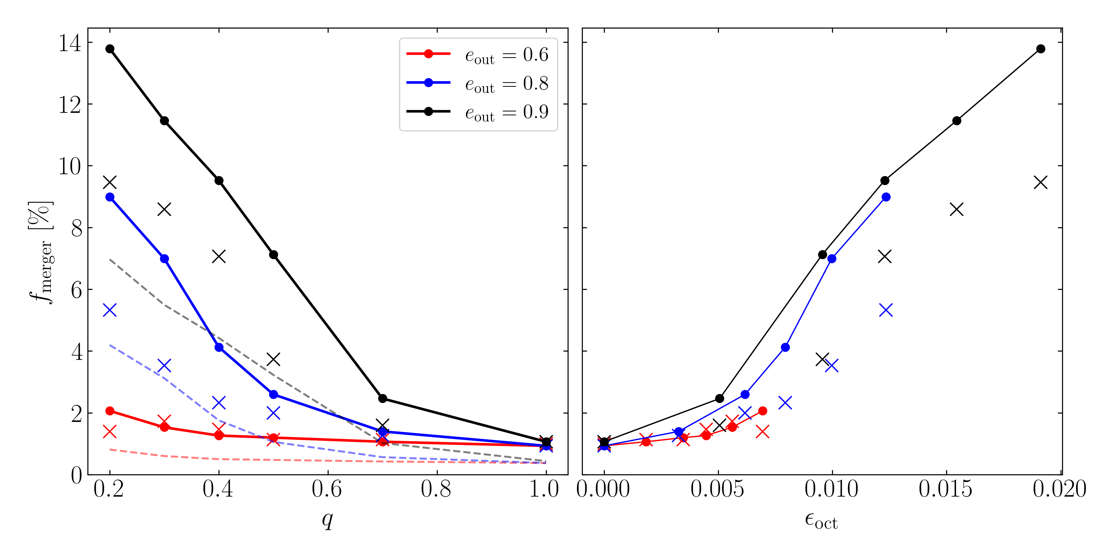
Figure 10: Same as Fig. 9 but for $a_{0}=50\;\mathrm{AU}$.

4.2 Merger Fraction for a Distribution of Tertiary Eccentricities

For a distribution of tertiary eccentricities, denoted $P\left(e_{\rm out}\right)$, the merger fraction is given by

$$\eta_{\rm merger}(q) =\int\mathrm{d}e_{\rm out}\;P\left(e_{\rm out}\right)f_{\rm merger}\left(q,e_{\rm out}\right),$$

$$=\int\limits\mathrm{d}e_{\rm out}\;\frac{P\left(e_{\rm out}\right)}{2}\int\limits_{-1}^{1}\mathrm{d}\cos I_{0}\;P_{\rm merger}\left(I_{0};q,e_{\rm out}\right).$$ (29)

We consider two possible $P(e_{\rm out})$ with $e_{\rm out}\in[0,0.9]$: (i) a uniform distribution, $P\left(e_{\rm out}\right)=\textrm{constant}$, and (ii) a thermal distribution, $P\left(e_{\rm out}\right)\propto e_{\rm out}$.

The top panel of Fig. 11 shows $\eta_{\rm merger}$ (black dots) for the fiducial triple systems (with the same parameters as in Figs. 4–7). For each $q$, the integral in Eq. (29) is computed using $1000$ realizations of random $e_{\rm out}$, $\cos I_{0}$, $\omega$, $\omega_{\rm out}$, and $\Omega$. Not surprisingly, we see $\eta_{\rm merger}$ increases with decreasing $q$. When $q$ is small, a thermal distribution of $e_{\rm out}$ tends to yield higher $\eta_{\rm merger}$ than does a uniform distribution. We also compute the merger fraction using the semi-analytical merger probability of Eq. (24) on a dense grid of initial conditions uniformly sampled in $e_{\rm out}$ and $\cos I_{0}$; the result is shown as the blue dotted line in Fig. 11, which is in good agreement with the uniform-$e_{\rm out}$ simulation result (black).

To characterize the properties of merging binaries, the middle and bottom panels of Fig. 11 show the distributions of merger times and merger eccentricities (at both the LISA and LIGO bands) for different mass ratios. To obtain the LISA and LIGO band eccentricities (with GW frequency equal to $0.1\;\mathrm{Hz}$ and $10\;\mathrm{Hz}$ respectively), the inner binaries are evolved from when they reach $0.005a_{0}$ (at which point we terminate the integration of the triple system evolution as the inner binary’s evolution is decoupled from the tertiary; see Eq. 15) to physical merger using Eqs. (13–14). While the LIGO band eccentricities are all quite small ($\lesssim 10^{-3}$), the LISA band eccentricities (at $0.1\;\mathrm{Hz}$) are significant, with median $\gtrsim 0.2$ for $q\lesssim 0.5$. We note that these eccentricities are generally smaller than those found in the population studies of Liu et al. (2019a). This is because in this paper we consider only sufficiently hierarchical systems for which double-averaged evolution equations are valid, whereas Liu et al. (2019a) included a wider range of triple hierarchies and had to use $N$-body integrations to evolve some of the systems.

For comparison, Figure 12 shows the results when $a_{\rm out,eff}=5500\;\mathrm{AU}$ (instead of $a_{\rm out,eff}=3600\;\mathrm{AU}$ for Fig. 11) with all other parameters unchanged. While $\eta_{\rm merger}$ is lower than it is for $a_{\rm out,eff}=3600\;\mathrm{AU}$, there is still a large increase of $\eta_{\rm merger}$ with decreasing $q$. Since Eq. (26) is still satisfied, this is expected.

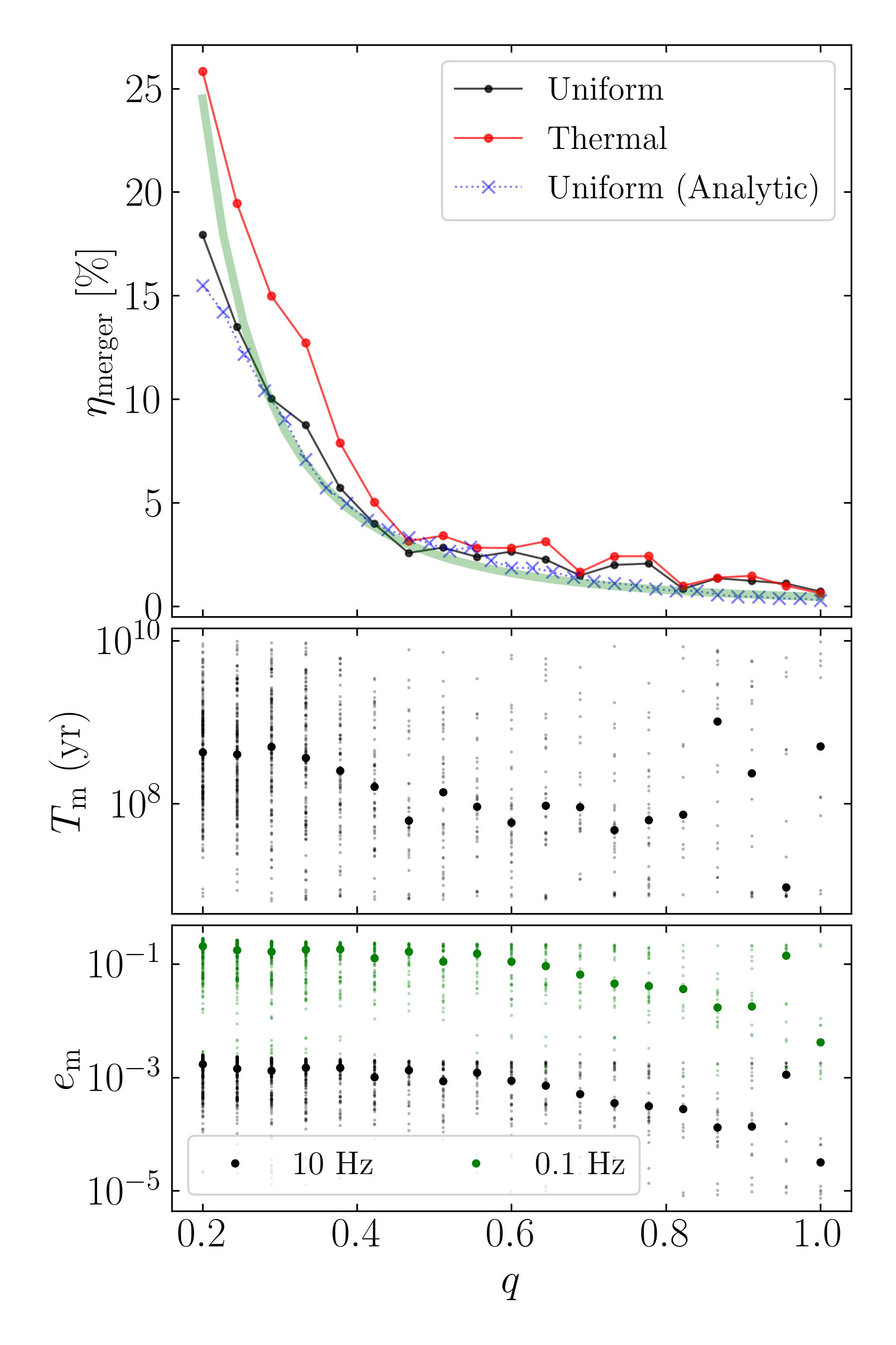
Figure 11: Upper panel: Binary BH merger fraction as a function of mass ratio $q$ for the fiducial triple systems (with parameters the same as in Figs. 4–7), assuming random mutual inclinations (uniform in $\cos I_{0}$), and either uniform (black dots) or thermal distribution (red dots) for the tertiary eccentricity distribution [with $e_{\rm out}\in[0,0.9]$]. These are obtained numerically using Eq. (29) by sampling $1000$ combinations of $e_{\rm out}$, $\cos I_{0}$, $\omega$, $\omega_{\rm out}$, and $\Omega$. The blue dotted line is the semi-analytical result obtained by applying Eq. (24) in Eq. (29) (evaluated using a dense uniform grid of $\cos I_{0}$ and $e_{\rm out}$). The thick green line is a power-law fit to the analytical $\eta_{\rm merger}$ with a power law index of $-2.5$. Middle panel: Merger times of successful mergers for a uniform $e_{\rm out}$ distribution (the median is denoted with the large black dot). Bottom panel: Merging binary eccentricities (again, for a uniform $e_{\rm out}$ distribution) in the LISA band ($0.1\;\mathrm{Hz}$; green) and in the LIGO band ($10\;\mathrm{Hz}$; black), with medians marked with large dots.

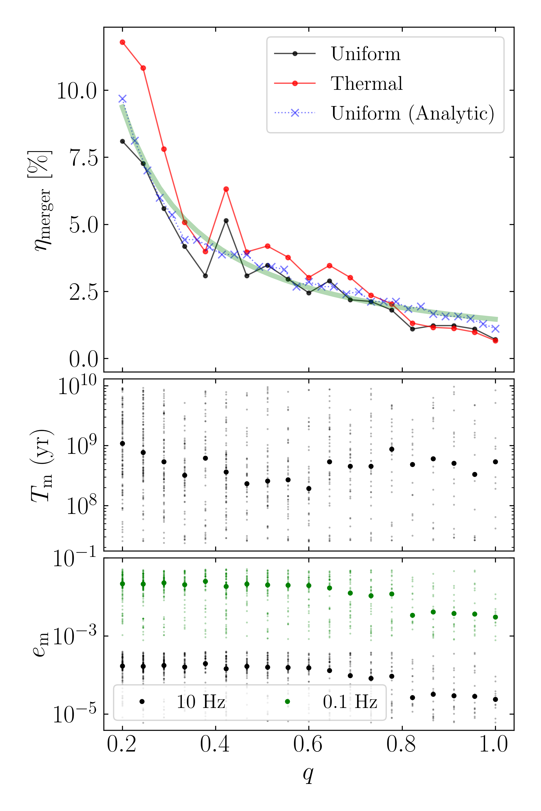
Figure 12: Same as Fig. 11 but for $a_{\rm out,eff}=5500\;\mathrm{AU}$. The power law index of the fit to the analytical $\eta_{\rm merger}$ is $-1.15$.

4.3 $q\ll 1$ Limit

For fixed $m_{12}$ (and other parameters), even though the octupole strength $\epsilon_{\rm oct}$ increases as $q$ decreases, the efficiency of GW radiation also decreases. It is therefore natural to ask at what $q$ these competing effects become comparable and the merger fraction is maximized. We show that this does not happen until $q$ is extremely small.

We see from Figs. 4–7 that $e_{\lim}>e_{\rm os}$ for our fiducial triple systems. Indeed, from Eq. (26), we see that even for $q$ as small as $10^{-5}$, the condition $e_{\lim}>e_{\rm os}$ is satisfied. This implies that most binaties execute one-shot mergers when undergoing an orbit flip. In addition, recall that the characteristic time for the binary to approach $e_{\lim}$ can be estimated by Eq. (11), which, for our fiducial triple systems, is given by

$$t_{\rm ZLK,oct}\simeq{} 10^{8}\left(\frac{m_{12}}{50M_{\odot}}\right)^{1/2}\left(\frac{a_{\rm out,eff}}{3600\;\mathrm{AU}}\right)^{7/2}\left(\frac{a}{100\;\mathrm{AU}}\right)^{-2}$$

$$\times\left(\frac{m_{3}}{30M_{\odot}}\right)^{-1}\Bigg{[}\frac{1-q}{1+q}\frac{e_{\rm out}}{\sqrt{1-e_{\rm out}^{2}}}\Bigg{]}^{-1/2}\;\mathrm{yr}.$$ (30)

Since $t_{\rm ZLK,oct}\ll 10\;\mathrm{Gyr}$, this implies that the octupole-ZLK-induced binary merger fractions are primarily determined by what initial conditions would lead to extreme eccentricity excitation and only weakly depend on the GW radiation rate. Indeed, Eq. (26) shows that, while $e_{\lim}>e_{\rm os}$ is indeed violated if $q$ is decreased sufficiently, the dependence is extremely weak. Thus, $\eta_{\rm merger}$ is expected to be very nearly constant for all physically relevant values of $q$, as can be seen in Fig. 13.

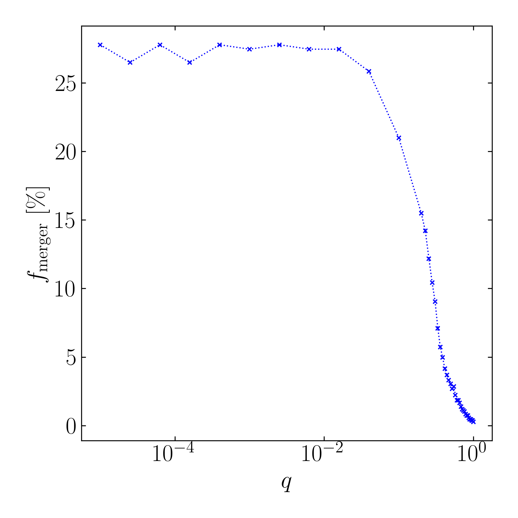
Figure 13: Same as blue dashed line of the top panel of Fig. 11 but extended to very small $q$. Due to the very weak $q$ dependence in Eq. (26), $f_{\rm merger}$ is expected to depend very weakly on $q$ when $q\ll 1$ (such that $\epsilon_{\rm oct}$ is approximately constant), which agrees with the simulation results.

4.4 Limitations of semi-analytic Calculation

It can be seen in Fig. 9 that the semi-analytical merger fractions are systematically lower than the values obtained from the direct simulations. One reason that this discrepancy arises is because the non-dissipative simulations used to compute $e_{\rm eff}$ and $e_{\max}$ are only run for $2000t_{\rm LK}\approx 3\;\mathrm{Gyr}$, while the full simulations including GW dissipation are run for $10\;\mathrm{Gyr}$. Owing to the chaotic nature of the octupole-order ZLK effect, this means that, if an initial condition leads to extreme eccentricities only after many Gyrs, then $e_{\rm eff}$ and $e_{\max}$ are underpredicted by the non-dissipative simulations. Additionally, there are times when eccentricity vector of the inner binary is librating, during which orbit flips are strongly suppressed (Katz et al., 2011). Since the librating phase can last an unpredictable amount of time, this suggests that the semi-analytical merger criteria can become more complete as the integration time is increased.

We quantify the “completeness” of the semi-analytical merger fraction via the ratio $f_{\rm merger}^{\rm an}/f_{\rm merger}$ as a function of non-dissipative integration time. We focus on the fiducial triple systems for demonstrative purposes and compute the completeness for each of the $q$ and $e_{\rm out}$ combinations shown in Fig. 9. Figure 14 shows the completeness for each of these simulations in light grey lines and their mean in the thick black line. We see that the completeness is still increasing even as the non-dissipative simulation time is increased to $2000t_{\rm ZLK}$, so we expect that even longer integration times would give even better agreement with the dissipative simulations.

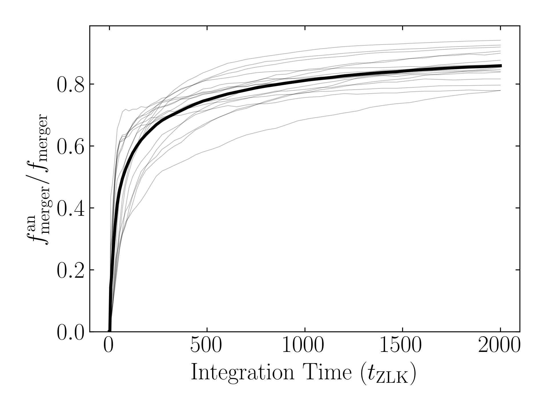
Figure 14: Completeness of the semi-analytical merger fraction, defined as $f_{\rm merger}^{\rm an}/f_{\rm merger}$, as a function of the integration time used for the non-dissipative simulations, in the fiducial parameter regime while $e_{\rm out}$ is fixed at a few values. The thin grey lines indicate the completeness for particular combinations of $(q,e_{\rm out})$, and the thick black line denotes their average. We see that completeness is still increasing as the integration time approaches $2000t_{\rm ZLK}\approx 3\;\mathrm{Gyr}$.

5 Mass Ratio Distribution of Merging BH Binaries

In Section 4, we have calculated the binary BH merger fractions $f_{\rm merger}$ and $\eta_{\rm merger}$ as a function of the mass ratio $q$ for some representative triple systems. To determine the distribution in $q$ and $m_{12}$ (total mass) of the merging binaries, we would need to know both the initial distribution in $q$, $m_{12}$ and $a_{0}$ of the inner BH binaries and the distribution in $m_{3}$, $a_{\rm out}$ and $e_{\rm out}$ of the outer binaries, denoted by:

$$\frac{\mathrm{d}F}{\mathrm{d}q\mathrm{d}m_{12}\mathrm{d}a_{0}},\quad\frac{\mathrm{d}F_{\rm out}}{\mathrm{d}m_{3}\mathrm{d}a_{\rm out}\mathrm{d}e_{\rm out}}.$$ (31)

The distribution in $q$ and $m_{12}$ of the merging binaries is then

$${\mathrm{d}F_{\rm merger}\over\mathrm{d}q\mathrm{d}m_{12}}=\int\!\mathrm{d}a_{0}\mathrm{d}m_{\rm out}\mathrm{d}a_{\rm out}\mathrm{d}e_{\rm out}\,{\mathrm{d}F\over\mathrm{d}q\mathrm{d}m_{12}\mathrm{d}a_{0}}$$

$$\qquad\times{\mathrm{d}F_{\rm out}\over\mathrm{d}m_{3}\mathrm{d}a_{\rm out}\mathrm{d}e_{\rm out}}\,f_{\rm merger}(q,e_{\rm out};m_{12},a_{0},m_{3},a_{\rm out},e_{\rm out}),$$ (32)

where $f_{\rm merger}$ is given by Eq. (27) (assuming random mutual inclinations between the inner and outer binaries), and we have spelled out its dependence on various system parameters. Some examples of $f_{\rm merger}$ are shown in Figs. 9–10. If we further specify the eccentricity distribution of the outer binaries, we have

$${\mathrm{d}F_{\rm merger}\over\mathrm{d}q\mathrm{d}m_{12}}=\int\!\mathrm{d}a_{0}\mathrm{d}m_{3}\mathrm{d}a_{\rm out}\,{\mathrm{d}F\over\mathrm{d}q\mathrm{d}m_{12}\mathrm{d}a_{0}}$$

$$\qquad\times{\mathrm{d}F_{\rm out}\over\mathrm{d}m_{3}\mathrm{d}a_{\rm out,eff}}\,\eta_{\rm merger}(q;m_{12},a_{0},m_{3},a_{\rm out,eff}),$$ (33)

where $\eta_{\rm merger}$ is given by Eq. (29). Some examples of $\eta_{\rm merger}$ are shown in the top panels of Figs. 11–12.

Clearly, to properly evaluate Eq. (32) or (33) would require large population synthesis calculations and in any case would involve significant uncertainties, a task beyond the scope of this paper. For illustrative purposes, we consider the fiducial triple systems as studied in Section 4, and estimate the mass-ratio distribution of BH mergers as

$${\mathrm{d}F_{\rm merger}\over\mathrm{d}q}\sim{\mathrm{d}F\over\mathrm{d}q}\,\eta_{\rm merger}(q).$$ (34)

5.1 Initial $q$-distribution of BH Binaries

The initial mass-ratio distribution of BH binaries, $\mathrm{d}F/\mathrm{d}q$, is uncertain. It can be derived from the the mass distributions of of main-sequence (MS) binaries, together with the MS mass ($m_{\rm ms}$) to BH mass ($m$) relation.

For the distribution of MS binary masses, we assume that each MS component mass is drawn from a Salpeter-like initial mass function (IMF) independently, with

$${\mathrm{d}F_{\rm ms}\over\mathrm{d}m_{\rm ms}}\propto m_{\rm ms}^{-\alpha},$$ (35)

in the range $m_{\min}\leq m_{\rm ms}\leq m_{\max}$. Note in this case the MS binary mass-ratio distribution is (for $q\leq 1$)

$${\mathrm{d}F_{\rm ms}\over\mathrm{d}q}\propto q^{\alpha-2}\left[1-\left(\frac{q}{q_{\min}}\right)^{2-2\alpha}\right],$$ (36)

where $q_{\min}=m_{\min}/m_{\max}$ is the minimum possible binary mass ratio (this is a generalization of the result of Tout, 1991). We consider two representative values of $\alpha$: (i) $\alpha=2.35$, the canonical Salpeter IMF (Salpeter, 1955), and (ii) $\alpha=2$, resulting in a uniform $q$ distribution (for $q\gtrsim 2q_{\min}$). The latter case is consistent with observational studies of the mass ratio of high-mass MS binaries (Sana et al., 2012; Duchêne & Kraus, 2013; Kobulnicky et al., 2014; Moe & Di Stefano, 2017).

To obtain $\mathrm{d}F/\mathrm{d}q$, we compute the BH binary mass ratio when each main sequence mass $m_{\rm ms}$ is mapped to its corresponding BH mass $m$. This mapping is taken from Spera & Mapelli (2017) for the mass range $25M_{\odot}\leq m_{\rm ms}\leq 117M_{\odot}$. We consider both the case where $Z=0.02$ (“high $Z$”) and where $Z=2.0\times 10^{-4}$ (“low $Z$”), the two limiting metallicities used in Spera & Mapelli (2017). We can then numerically compute $\mathrm{d}F/\mathrm{d}q$ by sampling masses for stellar binaries from the IMF, translating these into BH masses, then calculating the resulting BH mass ratios for each binary. The upper panel of Fig. 15 shows the $\mathrm{d}F/\mathrm{d}q$ obtained via this procedure for a Salpeter IMF ($\alpha=2.35$) when sampling $10^{5}$ MS binaries for each metallicity. In the lower four panels, we also show $\mathrm{d}F/\mathrm{d}q$ restricted to particular ranges of $m_{12}$. Note that the distributions differ significantly among the $m_{12}$ ranges and also between the two metallicities. Figure 16 shows the case when $\alpha=2$, which mostly resembles Fig. 15.

5.2 $q$-distribution of Merging BH Binaries

Using the results of Section 5.1, we can also estimate the mass ratio distribution of merging BHs using Eq. (34). We consider representative triple systems considered in Section 4: for $\eta_{\rm merger}$, we use a simple approximation that lies roughly between the two cases shown in Figs. 11–12:

$$\eta_{\rm merger}(q)\approx 0.2\times\left[\max\left(q,0.2\right)\right]^{-2}.$$ (37)

The results for $\mathrm{d}F_{\rm merger}/\mathrm{d}q$ are displayed as the dotted curves in Figs. 15–16 in each panel. Broadly speaking, $\mathrm{d}F_{\rm merger}/\mathrm{d}q$ peaks around $q\sim 0.3$ for low-Z systems, and around $q\sim 0.4$ for high-Z systems, the latter reflecting the peak in the initial BH binary q-distribution. Also note that $\mathrm{d}F_{\rm merger}/\mathrm{d}q$ can be quite different for different $m_{12}$ ranges. For example, merging BH binaries with $m_{12}>42M_{\odot}$ are only produced in low-Z systems, and $\mathrm{d}F_{\rm merger}/\mathrm{d}q$ peaks around $q\sim 0.3$ for $m_{12}\in[42,67]M_{\odot}$, and is roughly uniform between $q\sim 0.2$ to $1$ for $m_{12}\gtrsim 67M_{\odot}$.

We emphasize that these results for $\mathrm{d}F_{\rm merger}/\mathrm{d}q$ refer to the representative triple systems studied in Sections 2–4, and thus should be considered for illustrative purposes only. As noted above, the merger fraction $\eta_{\rm merger}$ depends on various parameters of the triple systems. While we have not attempted to quantify $\eta_{\rm merger}$ for all possible triple system parameters, it is clear that the principal finding of Section 4 (i.e., $\eta_{\rm merger}$ increases with decreasing $q$) applies only for systems with sufficiently strong octupole effects. In fact, from Figs. 9 and 10 we can estimate that the octupole-induced feature in $\eta_{\rm merger}$ becomes prominent only when $\epsilon_{\rm oct}\gtrsim 0.005$, or equivalently

$${a\over a_{\rm out,eff}}\gtrsim 0.005\left({1+q\over 1-q}\right){\sqrt{1-e_{\rm out}^{2}}\over e_{\rm out}}\simeq{0.01\over e_{\rm out}},$$ (38)

where in the second step we have used $q\sim 0.5$ and $e_{\rm out}\sim 0.6$. When this condition is satisfied, the inner binary can usually also undergo a one-shot merger (see Eq. 26), leading to strong dependence of the merger fraction on $q$. For triple systems with $a/a_{\rm out,eff}\lesssim 0.01$ (such as the case when the tertiary is a supermassive BH with $m_{3}\gtrsim 10^{6}m_{12}$), the octupole effect is unimportant (see the discussion following Eq. 2), and we expect the merger fraction to be almost independent of $q$. Indeed, an analytical fitting formula for BH mergers induced by pure quadrupole-ZLK effect shows $\eta_{\rm merger}\propto\mu^{0.16}\propto q^{0.16}/(1+q)^{0.32}$ (see Eq. 53 of Liu & Lai, 2018, or Eq. 26 of Liu & Lai, 2021). For such systems, we expect $\mathrm{d}F_{\rm merger}/\mathrm{d}q$ to be mainly determined by the initial $q$-distribution of BH binaries at their formation.

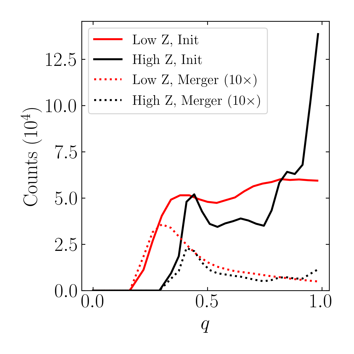
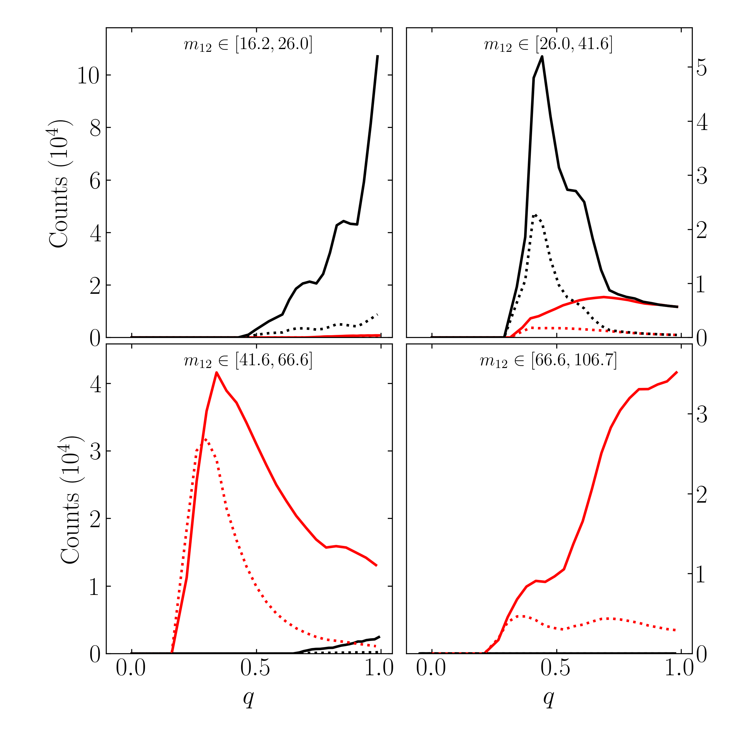
Figure 15: Mass ratio distributions of the initial BH binaries (solid lines) and merging BH binaries (dotted lines) when using $\alpha=2.35$ for the MS stellar initial mass function (see Sections 5.1 and 5.2). Top panel: Distribution of binary mass ratio at formation and merger for all possible total binary BH masses. Each BH mass is obtained from the MS mass using the fitting formula of Spera & Mapelli (2017) for metallicities of $2\times 10^{-4}$ (Low Z) and $0.02$ (High Z), while the merger fraction of BH binaries is given by Eq. (37). To produce these distributions, $10^{5}$ initial MS binaries are used for each metallicity, and the number of merging BH binaries has been scaled up by a factor of $10$ for visibility. The counts refer to the number per $\Delta q=0.05$ bin. Bottom four panels: Same as the top panel but with specific ranges of $m_{12}$, the total BH mass of the binary (as labeled). Note that low-$m_{12}$ systems are mainly produced from high-Z MS binaries, while high-$m_{12}$ systems are mainly produced in low-Z MS binaries.

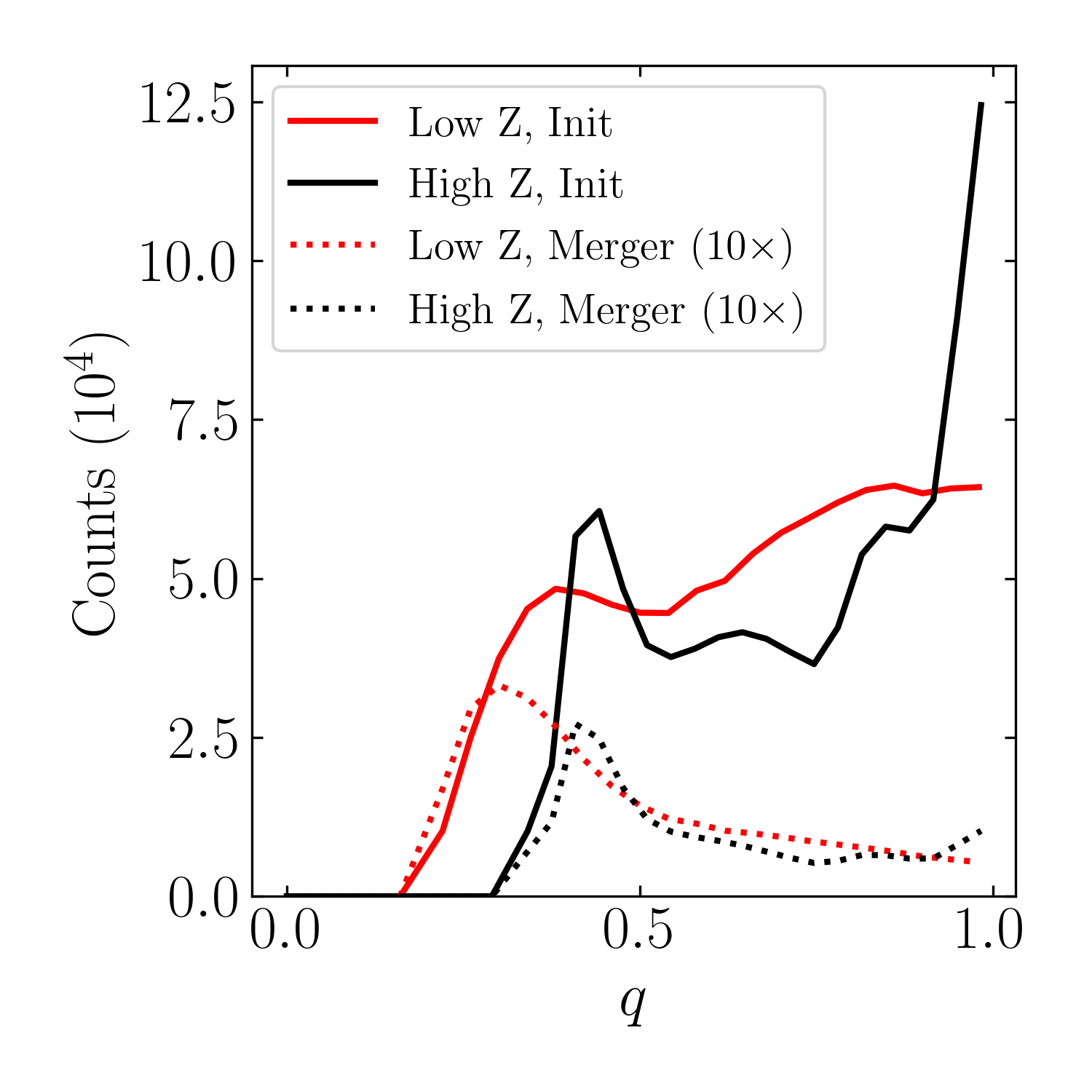
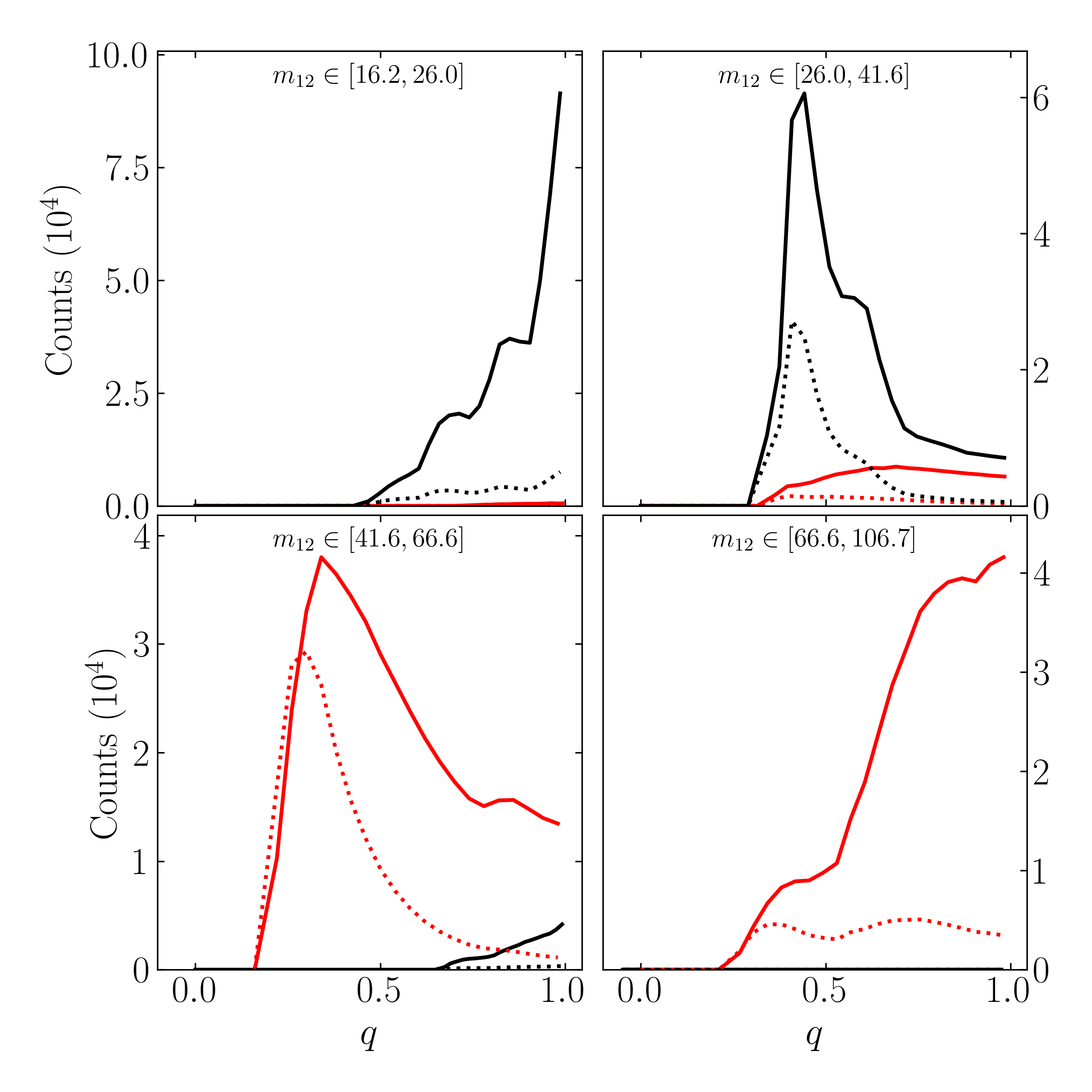
Figure 16: Same as Fig. 15 but for $\alpha=2$, i.e. a nearly uniform distribution of the main sequence binary mass ratio. The results are very similar to Fig. 15.

6 Summary and Discussion

We have studied the dynamical formation of merging BH binaries induced by a tertiary companion via the von Zeipel-Lidov-Kozai (ZLK) effect, focusing on the expected mass ratio distribution of merging binaries. The octupole potential of the tertiary, when sufficiently strong, can increase the inclination window and probability of extreme eccentricity excitation, and thus enhance the rate of successful binary mergers. Since the octupole strength $\epsilon_{\rm oct}\propto(1-q)/(1+q)$ (see Eq. 2) increases with decreasing binary mass ratio $q$, it is expected that ZLK-induced BH mergers favor binaries with smaller mass ratios. We quantify the dependence of the merger fraction/probability on $q$ using a combination of numerical integrations and analytical calculations, based on the secular evolution equations for hierarchical triples. We develop new analytical criteria (Section 3.2) that allow us to determine, without full numerical integrations, whether an initial BH binary can undergo a “one-shot merger” or a more gradual merger under the influence of a tertiary companion. These allow us to compute the merger probability semi-analytically by only studying non-dissipative (i.e. no GWs) triple systems (see Eq. 24). We show that for hierarchical triples with semi-major axis ratio $a/a_{\rm out}\gtrsim 0.01-0.02$ (see Eq. 38), the BH binary merger fraction ($f_{\rm merger}$ or $\eta_{\rm merger}$) can increase by a larger factor (up to $\sim 20$) as $q$ decreases from unity to $0.2$ (see Figs. 9–13). When combined with a reasonable estimate of the mass ratio distribution of the initial BH binaries (Section 5.1), our results for the merger fraction suggest that the final merging BH binaries have an overall mass ratio distribution that peaks around $q=0.3$ or $0.4$, although very different distributions can be produced when restricting to specific ranges of total binary masses (see Figs. 15 and 16).

Taking our final results (Figs. 15 and 16) at face value, we tentatively conclude that the mass-ratio distribution $\mathrm{d}F_{\rm merger}/\mathrm{d}q$ of BH binary mergers induced by a comparable-mass companion is inconsistent with the current LIGO/VIRGO result (see Fig. 1), suggesting that such tertiary-induced mergers may not be the dominant formation channel for the majority of the detected LIGO/VIRGO events. However, there are at least two important issues/caveats to keep in mind:

(i) $\mathrm{d}F_{\rm merger}/\mathrm{d}q$ depends strongly on the initial mass-ratio distribution of BH binaries at their formation ($\mathrm{d}F/\mathrm{d}q$), which is uncertain and depends sensitively on the metalicity of the binary formation environment (see Section 5.1). It is also possible that the initial BH binary mass ratio distribution is much more skewed towards equal masses than what we found in Section 5.1 (e.g. if stellar binaries with significantly asymmetric masses become unbound due to mass loss and supernova kicks as their components become BHs). Such a distribution was found by population synthesis studies that include octupole-order ZLK effects and models of stellar evolution (e.g. Hamers et al., 2013; Toonen et al., 2018). These studies find that ZLK oscillations in stellar binaries with small $q$ can experience mass transfer and merge without forming a compact object binary; as a result, most compact object binaries form with large mass ratios. The prevalence of this phenomenon likely depends on the initial semimajor axes of the inner binaries. Further study would be required to understand the competition between this primordial large-$q$ enhancement and the elevated merger fractions for small $q$ found in the present study in an astrophysically realistic population.

(ii) When the tertiary mass $m_{3}$ is much larger than the BH binary mass $m_{12}$, as in the case of a supermassive BH tertiary, dynamical stability of the triple requires $a_{\rm out}\gg a$, which implies that the octupole effect is negligible ($\epsilon_{\rm oct}\ll 1$). For such triple systems, we expect the merger fraction to depend very weakly on the mass ratio, and the final $\mathrm{d}F_{\rm merger}/\mathrm{d}q$ to depend entirely on the initial $\mathrm{d}F/\mathrm{d}q$. Although the merger fraction of such “pure quadrupole” triples is small ($\lesssim 6\%$; see Eq. 53 of Liu & Lai, 2018), additional “external” effects can enhance the merger efficiency significantly [e.g., when the outer orbit experiences quasi-periodic torques from the galactic potential (Petrovich & Antonini, 2017; see also Hamers & Lai, 2017), or from the spin of a supermassive BH (Liu et al., 2019b)].

Near the completion of this paper, we became aware of the simultaneous work by Martinez et al. (2021), who study a similar topic using a population synthesis approach.

7 Acknowledgements

We thank the anonymous referee whose detailed review and comments greatly improved this paper. YS thanks Jiseon Min for useful discussions. This work has been supported in part by NSF grant AST1715246. YS is supported by the NASA FINESST grant 19-ASTRO19-0041. BL gratefully acknowledges support from the European Union’s Horizon 2020 research and innovation program under the Marie Sklodowska-Curie grant agreement No. 847523 ‘INTERACTIONS’.

8 Data Availability

The data referenced in this article will be shared upon reasonable request to the corresponding author.

Appendix A Origin of Octupole-Inactive Gap

We investigate the origin of the “octupole-inactive gap”, an inclination range near $I_{0}\approx 90^{\circ}$ for which $e_{\max}$ does not attain $e_{\lim}$ despite being in between two octupole-active windows. This gap was first identified in Section 2.3, and is seen in both the non-dissipative and full simulations with GW dissipation (see Figs. 4–8).

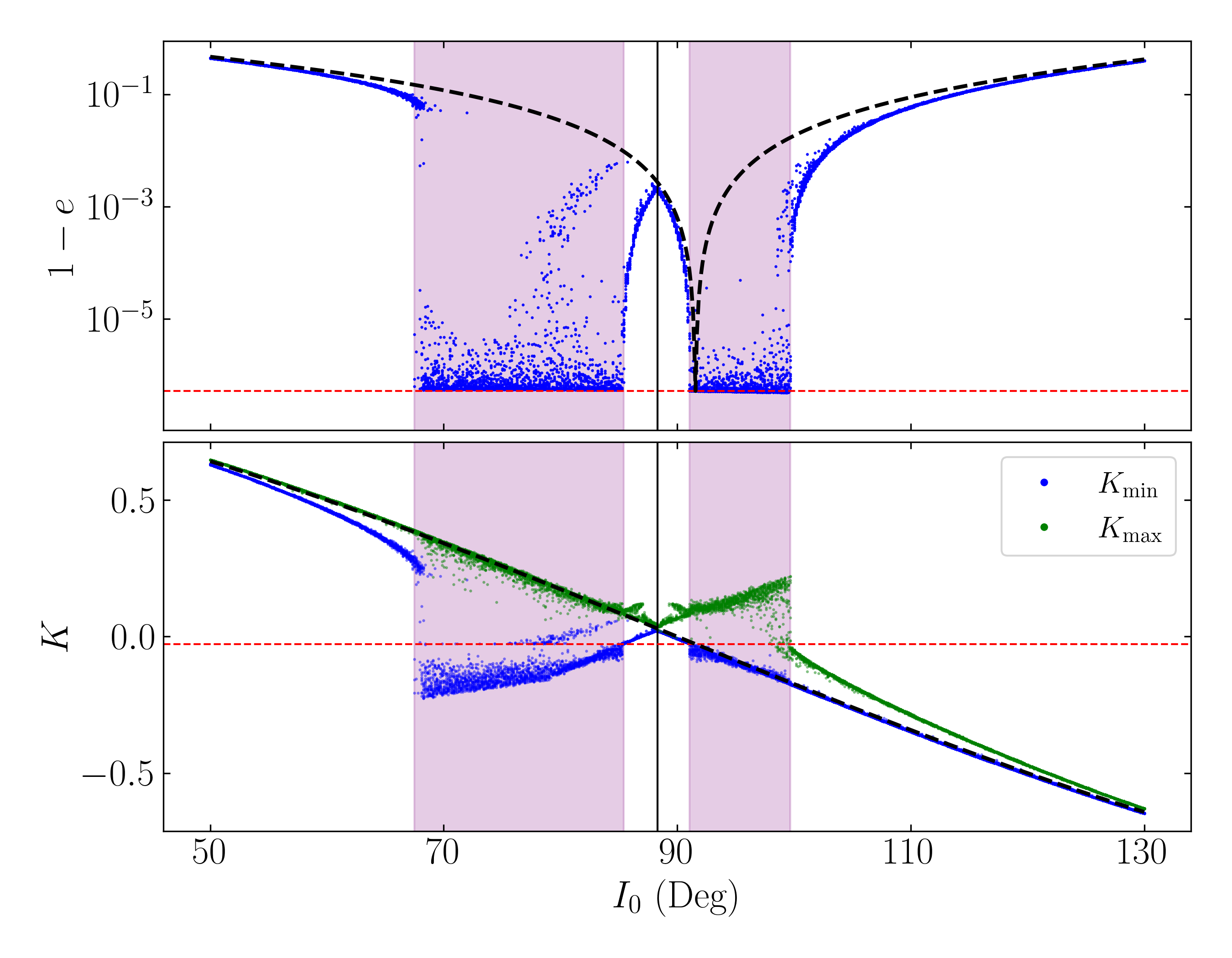
Figure 17: Octupole-active windows and amplitude of oscillation of $K$ (Eq. 4). Top panel: Maximum eccentricity $e_{\max}$ attained by the inner binary with initial tertiary inclination $I_{0}$ when integrated for $2000t_{\rm ZLK}$ (blue dots), reproduced from the top panel of Fig. 6. Also shown are $e_{\lim}$ (Eq. 9, horizontal red dashed line), the quadrupole-level result for $e_{\max}$ (Eq. 7, dashed black line), the empirically-determined center of the gap, located at $I_{0}\approx 88.32^{\circ}$ (vertical black line), and the inclinations that can lead to extreme eccentricities (shaded purple regions). Bottom panel: Minimum and maximum values of $K$, denoted $K_{\min}$ and $K_{\max}$, attained by the systems. Also shown are the initial $K$ for a given $I_{0}$ (black dashed line) and the critical $K_{\rm c}=-\eta/2$ for orbit flipping (horizontal red dashed line). The center of the octupole-inactive gap and the octupole-active windows are labeled as in the top panel.

To better understand this gap, we first review the mechanism by which extreme eccentricity excitation occurs. In the test-particle limit, Katz et al. (2011) showed that $K$ (Eq. 4) oscillates over long timescales when $\omega$, the argument of pericenter of the inner orbit, is circulating. This then leads to orbit flips (and extreme eccentricity excitation) between prograde and retrograde inclinations when $K$ changes signs: since $j(e)$ is nonnegative, the sign of $K$ determines the sign of $\cos I$. Katz et al. (2011) obtained coupled oscillation equations in $K$ and $\Omega_{\rm e}$, the azimuthal angle of the inner eccentricity vector in the inertial reference frame. The amplitude of oscillation of $K$ can then be analytically computed, and the octupole-active window (the range of $I_{0}$ over which orbit flips occur) is the region for which the range of these oscillations encompasses $K=0$ (Katz et al., 2011). When $\omega$ is librating instead, $\Omega_{\rm e}$ jumps by $\sim 180^{\circ}$ every ZLK cycle, and the oscillations in $K$ are suppressed.

In the finite-$\eta$ case, we commented in Section 2.3 that the relation between $K$ oscillations and extreme eccentricity excitation (and orbit flipping) can be generalized even when $\eta$ is nonzero. $K$ still oscillates over timescales $\gg t_{\rm ZLK}$ when $\omega$ is circulating, and if its range of oscillation contains $K_{\rm c}\equiv-\eta/2$, then the inner orbit flips, in the process attaining extreme eccentricities. To be precise, orbit flips are defined to be when the range of inclination oscillations changes from $\left(\cos I_{0}\right)_{-}<\cos I<\cos I_{0,\lim}$ to $\cos I_{0,\lim}<\cos I<\left(\cos I_{0}\right)_{+}$ or vice versa, where $\left(\cos I_{0}\right)_{\pm}$ are given by Eq. (10) and $I_{0,\lim}$ satisfies Eq. (8).

However, the range of oscillation of $K$ is more complex than it is in the test-particle limit. Figure 17 compares the behavior of $e_{\max}$ in the non-dissipative simulations (top panel; reproduced from the top panel of Fig. 6) to the range of oscillations in $K$ (bottom panel). Denote the center of the gap $I_{\rm 0,gap}$ (shown as the vertical black line in both panels of Fig. 17). Near $I_{\rm 0,gap}$, $K$ oscillates about $K(I_{\rm 0,gap})$, which is positive, and the oscillation amplitude goes to zero at $I_{\rm 0,gap}$. On the other hand, orbit flips (and extreme eccentricity excitation) are possible when the range of oscillation of $K$ encloses $K_{\rm c}$ (i.e., $K_{\min}<K_{\rm c}<K_{\max}$). The purple shaded regions in both panels of Fig. 17 illustrate this equivalence, as they show both the $e_{\lim}$-attaining inclinations in the top panel and the inclinations where $K_{\min}<K_{\rm c}<K_{\max}$ in the bottom panel. But since $K\left(I_{\rm 0,gap}\right)>0$ while $K_{\rm c}<0$, there will always be a range of $I_{0}$ about $I_{\rm 0,gap}$ for which the oscillation amplitude is smaller than $K\left(I_{\rm 0,gap}\right)-K_{\rm c}$, and orbit flips are impossible in this range. This range then corresponds to the octupole-inactive gap.

This analysis has simply pushed our lack of understanding onto a new quantity: why are $K$ oscillations suppressed in the neighborhood of $I_{\rm 0,gap}$? A quantitative answer to this question is beyond the scope of this paper, but for a qualitative understanding, we can examine the evolution of a system in the octupole-inactive gap. The left panel of Fig. 18 shows the same simulation as Fig. 3 but with an additional panel showing $\Omega_{\rm e}$, while the right panel shows a simulation with the same parameters except $I_{0}=88^{\circ}$, which is near $I_{\rm 0,gap}$ (see Fig. 17). The oscillations in $K$ (third panels) are much smaller for $I_{0}=88^{\circ}$ than for $I_{0}=93.5^{\circ}$, and no orbit flips occur. Most interestingly, the fourth panel shows that the evolution of $\Omega_{\rm e}$ is much less smooth than in Fig. 3, jumping at almost every other eccentricity maximum. Katz et al. (2011) have already pointed out that jumps in $\Omega_{\rm e}$ occur when $\omega$ is librating, rather than circulating.

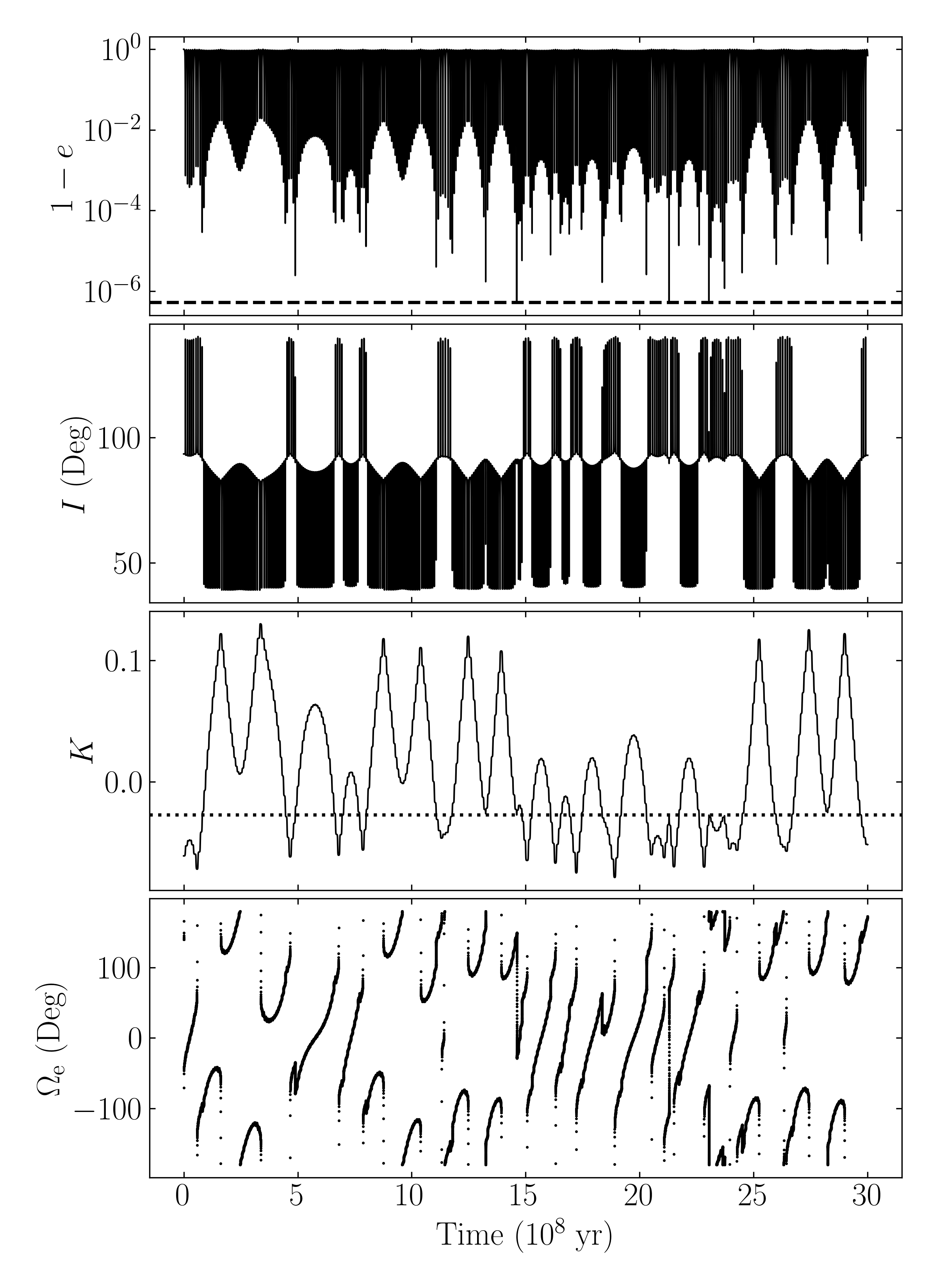
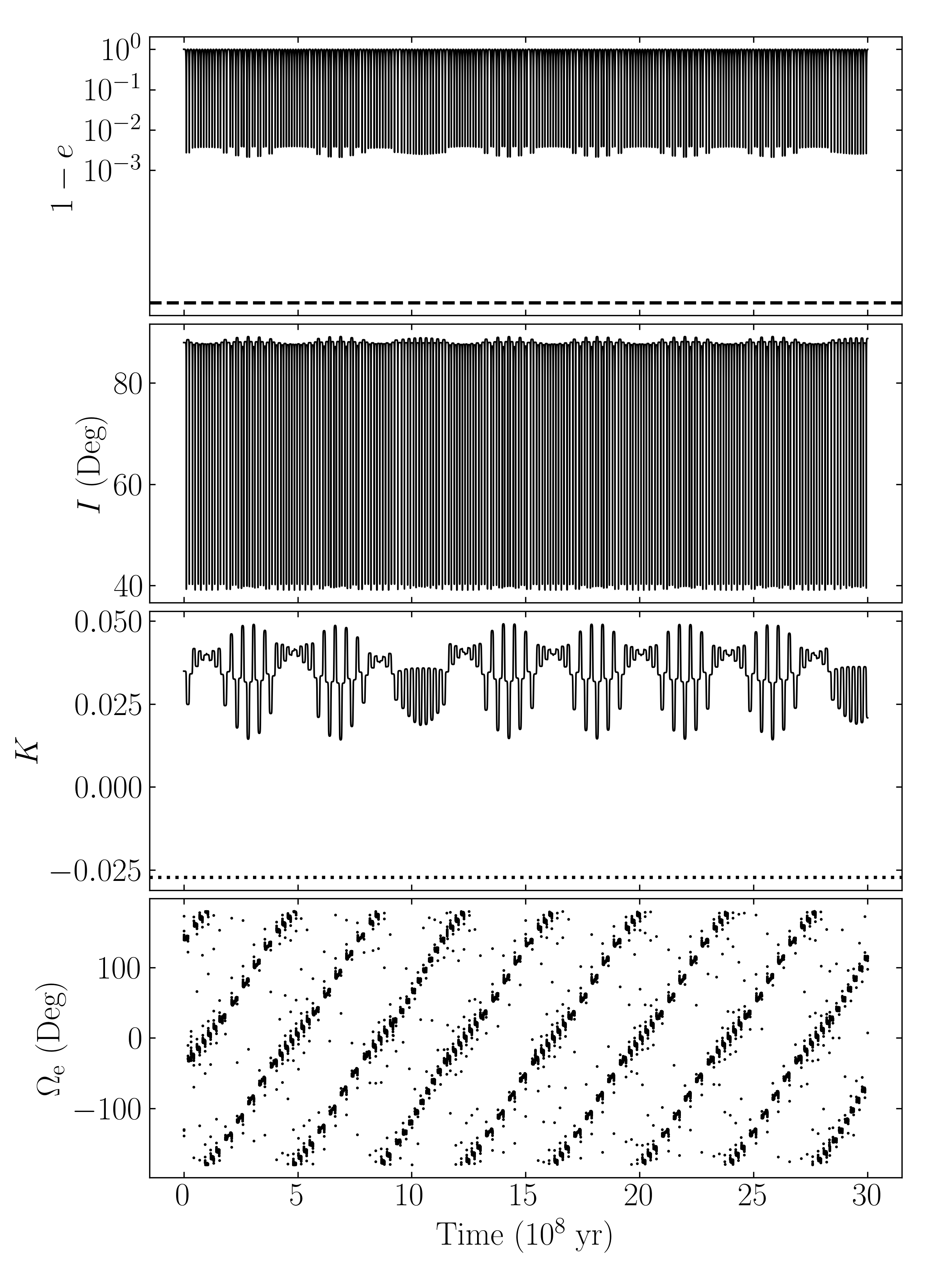
Figure 18: The left panel is the same as Fig. 3 but includes the evolution of the azimuthal angle of the eccentricity vector, $\Omega_{\rm e}$. The right panel is the same as the left but for $I_{0}=88^{\circ}$. For both of these examples, we have used $\omega_{0}=0$, but the evolution is similar for all $\omega_{0}$.

When the octupole-order terms are neglected, the circulation-libration boundary is a boundary in $e$-$\omega$ space: as long as the ZLK separatrix exists in the $e$-$\omega$ plane and $e_{0}>0$, then an initial $\omega_{0}=0$ causes $\omega$ to circulate, while an initial $\omega_{0}=\pi/2$ causes $\omega$ to librate (e.g., Kinoshita, 1993; Shevchenko, 2016). However, when including octupole-order terms, this picture breaks down. To illustrate this, for a range of $I_{0}$ and both $\omega_{0}=0$ and $\omega_{0}=\pi$, we evolve the fiducial system parameters for a single ZLK cycle, using $q=0.2$ as is used for Figs. 17 and 18, and consider both the dynamics with and without the octupole-order terms. Figure 19 gives the resulting changes in $\Omega_{\rm e}$ over a single ZLK period when the octupole-order effects are neglected (top) and when they are not (bottom). Two observations can be made: (i) $I_{\rm 0,gap}$ is approximately where $\Delta\Omega_{\rm e}=0$ for circulating initial conditions when neglecting octupole-order terms, and (ii) the inclusion of the octupole-order terms seem to cause $\Omega_{\rm e}$ to exclusively vary slowly ($\left|\Delta\Omega_{\rm e}\right|\ll 180^{\circ}$) except for $I_{\rm 0,gap}<I_{0}<I_{0,\lim}$. The former is plausible: if $K(I_{\rm 0,gap})$ is the location of an equilibrium in $K$-$\Omega_{\rm e}$ space, then it must satisfy $\Delta\Omega_{\rm e}=0$. The latter suggests that the assumption of circulation of $\omega$ in Katz et al. (2011) may be satisfied for many more initial conditions than the quadrupole-level analysis suggests, as long as they are not in octupole-inactive gap.

Finally, examination of the bottom panel of Fig. 17 suggests that the oscillation amplitude in $K$ grows roughly linearly with $\left|I_{0}-I_{\rm 0,gap}\right|$ in the vicinity of $I_{\rm 0,gap}$ (this may be because, in the test-particle limit, librating $\omega$ give oscillation amplitudes in $K$ that are higher-order in $K$ and $\Omega_{\rm e}$, as pointed out by Katz et al., 2011). Assuming this, the gap width can then be given by

$$\text{Gap Width}=2\left(I_{0,\lim}-I_{\rm 0,gap}\right).$$ (39)

This explains why the gap does not exist in the test-particle regime, as $I_{0,\lim}=I_{\rm 0,gap}=90^{\circ}$ by symmetry of the equations of motion.

It is clear from the preceding discussion and Fig. 19 that the octupole-order, finite-$\eta$ dynamics are complex, and our discussion can only be considered heuristic. Nevertheless, in the absence of a closed form solution to the octupole-order ZLK equations of motion or a full generalization of the work of Katz et al. (2011), they provide a preliminary understanding of the octupole-inactive gap.

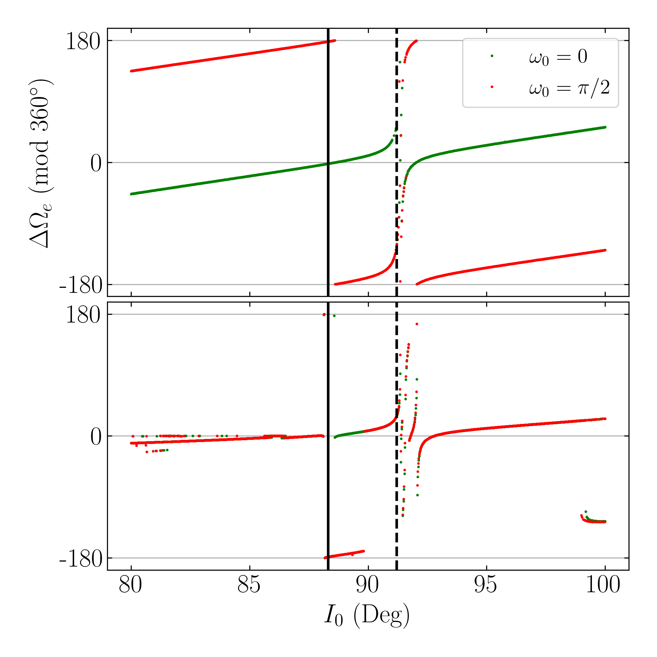
Figure 19: Plot of $\Delta\Omega_{\rm e}$, the change in $\Omega_{\rm e}$ over a single ZLK cycle, for $q=0.2$ and the fiducial parameters using different initial conditions. In the top panel, octupole-order terms are neglected, while in the lower panel, they are not. The solid and dashed vertical black lines denote $I_{\rm 0,gap}$ and $I_{0,\lim}$ respectively.

References

- Abbott et al. (2020a) Abbott R., et al., 2020a, arXiv preprint arXiv:2010.14533
- Abbott et al. (2020b) Abbott R., et al., 2020b, The Astrophysical Journal Letters, 900, L13
- Anderson et al. (2016) Anderson K. R., Storch N. I., Lai D., 2016, Monthly Notices of the Royal Astronomical Society, 456, 3671
- Antognini (2015) Antognini J. M., 2015, Monthly Notices of the Royal Astronomical Society, 452, 3610
- Antonini & Perets (2012a) Antonini F., Perets H. B., 2012a, The Astrophysical Journal, 757, 27
- Antonini & Perets (2012b) Antonini F., Perets H. B., 2012b, The Astrophysical Journal, 757, 27
- Antonini et al. (2014) Antonini F., Murray N., Mikkola S., 2014, The Astrophysical Journal, 781, 45
- Antonini et al. (2017) Antonini F., Toonen S., Hamers A. S., 2017, The Astrophysical Journal, 841, 77
- Antonini et al. (2018) Antonini F., Rodriguez C. L., Petrovich C., Fischer C. L., 2018, Monthly Notices of the Royal Astronomical Society: Letters, 480, L58
- Banerjee et al. (2010) Banerjee S., Baumgardt H., Kroupa P., 2010, Monthly Notices of the Royal Astronomical Society, 402, 371
- Belczynski et al. (2010) Belczynski K., Dominik M., Bulik T., O’Shaughnessy R., Fryer C., Holz D. E., 2010, The Astrophysical Journal Letters, 715, L138
- Belczynski et al. (2016) Belczynski K., Holz D. E., Bulik T., O’Shaughnessy R., 2016, Nature, 534, 512
- Blaes et al. (2002) Blaes O., Lee M. H., Socrates A., 2002, The Astrophysical Journal, 578, 775
- Dominik et al. (2012) Dominik M., Belczynski K., Fryer C., Holz D. E., Berti E., Bulik T., Mandel I., O’Shaughnessy R., 2012, The Astrophysical Journal, 759, 52
- Dominik et al. (2013) Dominik M., Belczynski K., Fryer C., Holz D. E., Berti E., Bulik T., Mandel I., O’Shaughnessy R., 2013, The Astrophysical Journal, 779, 72
- Dominik et al. (2015) Dominik M., et al., 2015, The Astrophysical Journal, 806, 263
- Downing et al. (2010) Downing J., Benacquista M., Giersz M., Spurzem R., 2010, Monthly Notices of the Royal Astronomical Society, 407, 1946
- Duchêne & Kraus (2013) Duchêne G., Kraus A., 2013, Annual Review of Astronomy and Astrophysics, 51, 269
- Ford et al. (2000) Ford E. B., Kozinsky B., Rasio F. A., 2000, The Astrophysical Journal, 535, 385
- Fragione & Bromberg (2019) Fragione G., Bromberg O., 2019, Monthly Notices of the Royal Astronomical Society, 488, 4370
- Fragione & Kocsis (2019) Fragione G., Kocsis B., 2019, Monthly Notices of the Royal Astronomical Society, 486, 4781
- Fragione & Loeb (2019) Fragione G., Loeb A., 2019, Monthly Notices of the Royal Astronomical Society, 486, 4443
- Gerosa et al. (2018) Gerosa D., Berti E., O’Shaughnessy R., Belczynski K., Kesden M., Wysocki D., Gladysz W., 2018, Phys. Rev. D, 98, 084036
- Gondán et al. (2018) Gondán L., Kocsis B., Raffai P., Frei Z., 2018, The Astrophysical Journal, 860, 5
- Hamers (2020a) Hamers A. S., 2020a, Monthly Notices of the Royal Astronomical Society, 494, 5492
- Hamers (2020b) Hamers A. S., 2020b, Monthly Notices of the Royal Astronomical Society, 500, 3481
- Hamers & Lai (2017) Hamers A. S., Lai D., 2017, Monthly Notices of the Royal Astronomical Society, 470, 1657
- Hamers et al. (2013) Hamers A. S., Pols O. R., Claeys J. S. W., Nelemans G., 2013, MNRAS, 430, 2262
- Hoang et al. (2018) Hoang B.-M., Naoz S., Kocsis B., Rasio F. A., Dosopoulou F., 2018, The Astrophysical Journal, 856, 140
- Katz et al. (2011) Katz B., Dong S., Malhotra R., 2011, Physical Review Letters, 107, 181101
- Kinoshita (1993) Kinoshita H., 1993, Celestial Mechanics and Dynamical Astronomy, 57, 359
- Kiseleva et al. (1996) Kiseleva L. G., Aarseth S. J., Eggleton P. P., de La Fuente Marcos R., 1996, in Milone E. F., Mermilliod J. C., eds, Astronomical Society of the Pacific Conference Series Vol. 90, The Origins, Evolution, and Destinies of Binary Stars in Clusters. p. 433
- Kobulnicky et al. (2014) Kobulnicky H. A., et al., 2014, The Astrophysical Journal Supplement Series, 213, 34
- Kozai (1962) Kozai Y., 1962, The Astronomical Journal, 67, 591
- Lei et al. (2018) Lei H., Circi C., Ortore E., 2018, Monthly Notices of the Royal Astronomical Society, 481, 4602
- Li et al. (2014) Li G., Naoz S., Holman M., Loeb A., 2014, The Astrophysical Journal, 791, 86
- Lidov (1962) Lidov M. L., 1962, Planetary and Space Science, 9, 719
- Lipunov et al. (1997) Lipunov V., Postnov K., Prokhorov M., 1997, Astronomy Letters, 23, 492
- Lipunov et al. (2017) Lipunov V., et al., 2017, Monthly Notices of the Royal Astronomical Society, 465, 3656
- Lithwick & Naoz (2011) Lithwick Y., Naoz S., 2011, The Astrophysical Journal, 742, 94
- Liu & Lai (2017) Liu B., Lai D., 2017, The Astrophysical Journal Letters, 846, L11
- Liu & Lai (2018) Liu B., Lai D., 2018, The Astrophysical Journal, 863, 68
- Liu & Lai (2019) Liu B., Lai D., 2019, Monthly Notices of the Royal Astronomical Society, 483, 4060
- Liu & Lai (2020) Liu B., Lai D., 2020, Physical Review D, 102, 023020
- Liu & Lai (2021) Liu B., Lai D., 2021, Monthly Notices of the Royal Astronomical Society, 502, 2049
- Liu et al. (2015) Liu B., Muñoz D. J., Lai D., 2015, Monthly Notices of the Royal Astronomical Society, 447, 747
- Liu et al. (2019a) Liu B., Lai D., Wang Y.-H., 2019a, The Astrophysical Journal, 881, 41
- Liu et al. (2019b) Liu B., Lai D., Wang Y.-H., 2019b, The Astrophysical Journal Letters, 883, L7
- Luo et al. (2016) Luo L., Katz B., Dong S., 2016, Monthly Notices of the Royal Astronomical Society, 458, 3060
- Martinez et al. (2021) Martinez M. A., Rodriguez C. L., Fragione G., 2021, arXiv preprint arXiv:2105.01671
- Miller & Hamilton (2002) Miller M. C., Hamilton D. P., 2002, The Astrophysical Journal, 576, 894
- Miller & Lauburg (2009) Miller M. C., Lauburg V. M., 2009, The Astrophysical Journal, 692, 917
- Moe & Di Stefano (2017) Moe M., Di Stefano R., 2017, The Astrophysical Journal Supplement Series, 230, 15
- Muñoz et al. (2016) Muñoz D. J., Lai D., Liu B., 2016, Monthly Notices of the Royal Astronomical Society, 460, 1086
- Naoz (2016) Naoz S., 2016, Annual Review of Astronomy and Astrophysics, 54, 441
- O’leary et al. (2006) O’leary R. M., Rasio F. A., Fregeau J. M., Ivanova N., O’Shaughnessy R., 2006, The Astrophysical Journal, 637, 937
- Olejak et al. (2020) Olejak A., Fishbach M., Belczynski K., Holz D. E., Lasota J.-P., Miller M. C., Bulik T., 2020, The Astrophysical Journal, 901, L39
- Peters (1964) Peters P. C., 1964, Physical Review, 136, B1224
- Petrovich & Antonini (2017) Petrovich C., Antonini F., 2017, The Astrophysical Journal, 846, 146
- Podsiadlowski et al. (2003) Podsiadlowski P., Rappaport S., Han Z., 2003, Monthly Notices of the Royal Astronomical Society, 341, 385
- Portegies Zwart & McMillan (2000) Portegies Zwart S. F., McMillan S. L. W., 2000, ApJ, 528, L17
- Randall & Xianyu (2018a) Randall L., Xianyu Z.-Z., 2018a, The Astrophysical Journal, 853, 93
- Randall & Xianyu (2018b) Randall L., Xianyu Z.-Z., 2018b, The Astrophysical Journal, 864, 134
- Rodet et al. (2021) Rodet L., Su Y., Lai D., 2021, The Astrophysical Journal, 913, 104
- Rodriguez et al. (2015) Rodriguez C. L., Morscher M., Pattabiraman B., Chatterjee S., Haster C.-J., Rasio F. A., 2015, Physical Review Letters, 115, 051101
- Rodriguez et al. (2016) Rodriguez C. L., Chatterjee S., Rasio F. A., 2016, Physical Review D, 93, 084029
- Rodriguez et al. (2018) Rodriguez C. L., Amaro-Seoane P., Chatterjee S., Rasio F. A., 2018, Physical Review Letters, 120, 151101
- Salpeter (1955) Salpeter E. E., 1955, The Astrophysical Journal, 121, 161
- Samsing & D’Orazio (2018) Samsing J., D’Orazio D. J., 2018, Monthly Notices of the Royal Astronomical Society, 481, 5445
- Samsing & Ramirez-Ruiz (2017) Samsing J., Ramirez-Ruiz E., 2017, The Astrophysical Journal Letters, 840, L14
- Sana et al. (2012) Sana H., et al., 2012, Science, 337, 444
- Shevchenko (2016) Shevchenko I. I., 2016, The Lidov-Kozai effect-applications in exoplanet research and dynamical astronomy. Astrophysics and Space Science Library Vol. 441, Springer
- Silsbee & Tremaine (2017) Silsbee K., Tremaine S., 2017, The Astrophysical Journal, 836, 39
- Spera & Mapelli (2017) Spera M., Mapelli M., 2017, Monthly Notices of the Royal Astronomical Society, 470, 4739
- Su et al. (2021) Su Y., Lai D., Liu B., 2021, Physical Review D, 103, 063040
- Toonen et al. (2018) Toonen S., Perets H., Hamers A., 2018, Astronomy & Astrophysics, 610, A22
- Tout (1991) Tout C. A., 1991, Monthly Notices of the Royal Astronomical Society, 250, 701
- von Zeipel (1910) von Zeipel H., 1910, Astronomische Nachrichten, 183, 345
- Wen (2003) Wen L., 2003, The Astrophysical Journal, 598, 419
- Ziosi et al. (2014) Ziosi B. M., Mapelli M., Branchesi M., Tormen G., 2014, Monthly Notices of the Royal Astronomical Society, 441, 3703