Offline Reinforcement Learning with Pseudometric Learning

Abstract

Offline Reinforcement Learning methods seek to learn a policy from logged transitions of an environment, without any interaction. In the presence of function approximation, and under the assumption of limited coverage of the state-action space of the environment, it is necessary to enforce the policy to visit state-action pairs close to the support of logged transitions. In this work, we propose an iterative procedure to learn a pseudometric (closely related to bisimulation metrics) from logged transitions, and use it to define this notion of closeness. We show its convergence and extend it to the function approximation setting. We then use this pseudometric to define a new lookup based bonus in an actor-critic algorithm: PLOff. This bonus encourages the actor to stay close, in terms of the defined pseudometric, to the support of logged transitions. Finally, we evaluate the method on hand manipulation and locomotion tasks.

1 Introduction

Reinforcement Learning (RL) has proven its ability to solve complex problems in recent years (Silver et al., 2016; Vinyals et al., 2019). Behind those breakthroughs, the adoption of RL in real-world systems remains challenging (Dulac-Arnold et al., 2019). Learning a policy by trial-and-error, while operating on the system, can be detrimental to the system where it is deployed (e.g., user satisfaction in recommendation systems or material damage in robotics) and is not guaranteed to lead to good performance (sparse rewards problems).

Nevertheless, in the setting where experiences were previously collected in an environment (logged transitions), one possible way of learning a policy is to mimic the policy that generated these experiences (Pomerleau, 1991). However, if these experiences come from different sources, with different degrees of desirability, naive imitation might lead to poor results. On the other hand, offline RL (or batch RL) (Lagoudakis & Parr, 2003; Ernst et al., 2005; Riedmiller, 2005; Levine et al., 2020), offers a setting where the policy is learned from the collected experiences. As it requires no interaction with the environment, offline RL is a promising direction for learning policies that can be deployed into systems.

Still, collected experiences typically only cover a subset of the range of possibilities in an environment (not every state is present; for a given state, not every action is taken). With function approximation, this is particularly problematic since actions not executed in the system can be assigned overly optimistic values (especially through bootstrapping), which leads to poor policies. To limit this extrapolation error, offline RL is typically incentivized to learn policies that are plausible in light of the collected experiences. In other words, offline RL methods need to learn policies that maximize their return, while making sure to remain close to the support of logged transitions.

This work introduces a new method for computing the closeness to the support by learning a pseudometric from collected experiences. This pseudometric, close to bisimulation metrics (Ferns et al., 2004), computes similarity between state-action pairs based on the expected difference in rewards when following specific sequences of actions. We show theoretical properties in the dynamic programming setting for deterministic environments as well as for the sampled setting. We further extend the learning of this pseudometric to the function approximation setting, and propose an architecture to learn it from collected experience. We define a new offline RL actor-critic algorithm: PLOff (Pseudometric Learning Offline RL), which computes a bonus through this learned pseudometric and uses it to filter admissible actions in the greedy step and penalizes non-admissible actions in the evaluation step. Finally, we lead an empirical study on the hand manipulation and locomotion tasks of the D4RL benchmark from Fu et al. (2020).

We make the following contributions: 1) we extend neural bisimulation metrics (Castro, 2020) to state-action spaces and to the offline RL setting and 2) we exploit this pseudometric to tackle the out-of-distribution extrapolation error of offline RL by adding a simple lookup bonus to a standard actor-critic algorithm and show that it compares favorably to state-of-the art offline RL methods.

2 Background

Reinforcement Learning.

We consider the classic RL setting (Sutton & Barto, 1998), formalized with Markov Decision Processes (MDPs). An MDP is a tuple $\mathcal{M}:=(\mathcal{S},\mathcal{A},r,P,\gamma)$, with $\mathcal{S}$ the state space, $\mathcal{A}$ the action space, $r:\mathcal{S}\times\mathcal{A}\mapsto\mathbb{R}$ the expected reward function, $P:\mathcal{S}\times\mathcal{A}\mapsto\mathcal{P}(\mathcal{S})$ the transition function which maps state-action pairs to distributions over the set of states $\mathcal{P}(\mathcal{S})$ and $\gamma$ the discount factor for which we assume $\gamma\in[0,1)$. A stationary deterministic policy $\pi$ is a mapping from states to actions (the following can easily be extended to stochastic policies). The value function $V^{\pi}$ of a policy $\pi$ is defined as the expected discounted cumulative reward from starting in a particular state and acting according to $\pi$: $V^{\pi}(s)=\mathop{\mathbb{E}}\big{(}\sum^{\infty}_{i=0}\gamma^{i}r(s_{i},\pi(s_{i}))|s_{0}=s)\big{)}$. The action-value function $Q^{\pi}$ is defined as the expected cumulative reward from starting in a particular state, taking an action and then acting according to $\pi$: $Q^{\pi}(s,a)=r(s,a)+\gamma\mathop{\mathbb{E}}\big{(}V^{\pi}(s^{\prime})\big{)}$. The Bellman (1957) operator $\mathcal{B}$ connects an action-value function $Q$ for the state-action pair $(s,a)$ to the action-value function in the subsequent state $s^{\prime}$: $\mathcal{B}^{\pi}(Q)(s,a):=r(s,a)+\gamma\mathop{\mathbb{E}}\big{(}Q(s^{\prime},\pi(s^{\prime}))\big{)}$. $Q^{\pi}$ is the (unique) fixed-point of this operator, and the difference between $Q(s,a)$ and its image through the Bellman operator $\|Q-\mathcal{B}^{\pi}Q\|$ is called a temporal difference error.

An optimal policy $\pi^{*}$ maximizes the value function $V^{\pi^{*}}$ for all states. In continuous state-action spaces, actor-critic methods (Konda & Tsitsiklis, 2000) are a common paradigm to learn a near-optimal policy. In this work we only consider deterministic policies; we justify this restriction by the fact that stochastic policies are desirable because of their side effect of exploration (Haarnoja et al., 2018), but in this case we want to learn a policy with near-optimal behavior without interaction with the environment. Therefore, we use the actor-critic framework of Silver et al. (2014). It consists in concurrently learning a parametrized policy $\pi_{\theta}$ and its associated parametrized action-value function $Q_{\omega}$. $Q_{\omega}$ minimizes a temporal difference error $\|Q_{\omega}(s,a)-r(s,a)-Q_{\bar{\omega}}(s^{\prime},\pi_{\theta}(s^{\prime}))\|$ (with $Q_{\bar{\omega}}$ a target action-value function, tracking $Q_{w}$), and $\pi_{\theta}$ maximizes the action-value function $Q_{\omega}(s,\pi_{\theta}(s))$.

In the classical RL setting, transitions $(s,a,s^{\prime},r)$ are sampled through interactions with the environment. In on-policy actor-critic methods (Sutton et al., 1999; Schulman et al., 2015), updates on $\pi_{\theta}$ and $Q_{\omega}$ are made as the policy gathers transitions by interacting in the environment. In off-policy actor-critic methods (Lillicrap et al., 2016; Haarnoja et al., 2018; Fujimoto et al., 2019), the transitions gathered by the policy are stored in a replay buffer and sampled using different sampling strategies (Lin, 1992; Schaul et al., 2015). These off-policy methods extend to the offline RL setting quite naturally. The difference is that in the offline RL setting, transitions are not sampled through interactions from the environment, but from a fixed dataset of transitions.

Throughout the paper $\mathcal{D}=\{(s_{i},a_{i},r_{i},s^{\prime}_{i})\}_{1:N}$ is the dataset of $N$ transitions collected in the considered environment. To ease notations we write $s\sim\mathcal{D}$, $s,a\sim\mathcal{D}$, $r\sim\mathcal{D}$ to indicate that a transition $(s,a,s^{\prime},r)$ is sampled at random from this dataset, and that we only consider the associated state $s$, state-action pair $(s,a)$ or reward $r$ respectively.

Pseudometric in MDPs.

A core issue in RL is to define a meaningful metric between states or state-action pairs (Le Lan et al., 2021). Consider for example a maze, two states could be close according to the Euclidean distance, but far away in terms of the minimal distance an agent would have to travel to join one state from the other (due to walls). In this case, a relevant metric is the distance in the graph formed from state transitions induced by the MDP (Mahadevan & Maggioni, 2007). We consider the following relaxed notion of metric:

Definition 1 (Pseudometric).

Given a set $M$, a pseudometric is a function $d:M\times M\mapsto\mathbb{R}_{+}$ such that, $\forall x,y,z\in M$, we have $d(x;x)=0$, $d(x;y)=d(y;x)$, $d(x;z)\leq d(x;y)+d(y;z)$.

In the context of Markov Decision Processes, bisimulation relations (Givan et al., 2003) are a form of state abstraction (Li et al., 2006), based on an equivalence relation. They are defined by the following recurrent definition: two states are bisimilar if they yield the same expected reward and transition to bisimulation equivalence classes with equal probability. This definition is too restrictive to be useful in practice. Ferns et al. (2004) introduce bisimulation metrics which are pseudometrics that soften the concept of bisimulation relations. Bisimulation metrics are defined on the state space $\mathcal{S}$. Denote $\mathbb{M}_{\mathcal{S}}$ the set of pseudometrics on $\mathcal{S}$. The bisimulation metric is the (unique) fixed point of the operator $\mathcal{F_{\mathcal{S}}}$ defined as:

$$\mathcal{F}_{\mathcal{S}} (d)(s;t):=$$ (1)

$$\max_{a\in\mathcal{A}}\Big{(}|r(s,a)-r(t,a)|+\gamma\mathcal{W}_{1}(d)(P(s,a),P(t,a))\Big{)}$$ (2)

where $\mathcal{W}_{1}(d)$ is the 1-Wasserstein distance (Villani, 2008) with the distance between states measured according to the pseudometric $d$. Therefore, the bisimulation metric is the limit of the repeated application of the sequence $\big{(}\mathcal{F_{\mathcal{S}}}^{n}(d_{0})\big{)}_{n\in\mathbb{N}}$ for any initial $d_{0}\in\mathbb{M_{\mathcal{S}}}$.

Although pseudometrics in MDPs have proven to be effective in some applications (Melo & Lopes, 2010; Kim & Park, 2018; Dadashi et al., 2021), they are usually hand-crafted or learned with ad-hoc strategies.

3 Method

We present the overall idea of our method in Sec. 3.1: an offline RL algorithm which is incentivized to remain close to the support of collected experiences using a pseudometric-based bonus. In Sec. 3.2 to 3.4, we present how to learn this pseudometric, from a theoretical motivation to a gradient-based method. We give practical considerations to derive the bonus in Sec. 3.5 and provide the resulting algorithm: PLOff, in Sec. 3.6.

3.1 Offline RL with lookup bonus

For the time being, let us assume the existence of a pseudometric $d$ on the state-action space $\mathcal{S}\times\mathcal{A}$. We can infer a distance $d_{\mathcal{D}}$ from a transition to the dataset $\mathcal{D}$:

$$d_{\mathcal{D}}(s,a)=\min_{\hat{s},\hat{a}\in\mathcal{D}}d(s,a;\hat{s},\hat{a}).$$ (3)

This distance to the dataset $\mathcal{D}$, also referred to as the projection distance, is simply the distance from $(s,a)$ to the nearest element of $\mathcal{D}$. It is central to our work since it defines the notion of closeness to the support of transitions $\mathcal{D}$. From $d_{\mathcal{D}}$, we can infer a bonus $b$ using a monotonically decreasing function $f:\mathbb{R}\mapsto\mathbb{R}$:

$$b(s,a)=f(d_{\mathcal{D}}(s,a)).$$ (4)

Note that the concept of a bonus is overloaded in RL; it typically applies to exploration strategies (Schmidhuber, 1991; Thrun, 1992; Bellemare et al., 2016). In our case, the bonus $b$ is opposite to exploration-based bonuses since it will encourage the policy to act similarly to existing transitions of the collected experiences $\mathcal{D}$. In other words, it prevents exploring too far from the dataset.

We adapt the actor-critic framework by adding the bonus to the actor maximization step and the critic minimization step (with difference multipliers $\alpha_{a}$ and $\alpha_{c}$). We learn a parametrized policy $\pi_{\theta}$ and its corresponding action-value function $Q_{\omega}$. In a schematic way, we sample transitions $(s,a,r,s^{\prime})\in\mathcal{D}$ and minimize the two following losses:

$$\text{(critic)}\;\;\min_{\omega}\| Q_{\omega}(s,a)-r(s,a)$$ (5)

$$-\gamma Q_{\bar{\omega}}(s^{\prime},\pi_{\theta}(s^{\prime}))-{\color[rgb]{0,0,1}\alpha_{c}b(s^{\prime},\pi_{\theta}(s^{\prime}))}\|,$$ (6)

$$\text{(actor)}\;\;\max_{\theta}Q_{\omega}(s,\pi_{\theta}(s))+{\color[rgb]{0,0,1}\alpha_{a}b(s,\pi_{\theta}(s))}.$$ (7)

This modification of the actor-critic framework is common in offline RL (Buckman et al., 2021). The bonus $b$ typically consists in a measure of similarity between an estimated behavior policy that generated $\mathcal{D}$ and the policy $\pi$ we learn (Fujimoto et al., 2018; Wu et al., 2019; Kumar et al., 2019).

3.2 Pseudometric Learning

To define a bonus $b$, we first learn a pseudometric $d$ on the state-action space $\mathcal{S}\times\mathcal{A}$ similarly to bisimulation metrics (Ferns et al., 2004, 2011, 2006), with the difference being that we are interested in pseudometrics in state-action space $\mathcal{S}\times\mathcal{A}$ rather than state space $\mathcal{S}$. We will show that the pseudometric $d$ we are interested in is the fixed point of an operator $\mathcal{F}$. In the following, we assume that the MDP is deterministic.

Let $\mathbb{M}$ be the set of bounded pseudometrics on $\mathcal{S}\times\mathcal{A}$. We define the operator $\mathcal{F}:\mathbb{M}\mapsto\mathbb{M}$ as follows: for two state-action pairs $(s_{1},a_{1})$ and $(s_{2},a_{2})$, that maps to next states $s^{\prime}_{1}$ and $s^{\prime}_{2}$ we have:

$$\mathcal{F}(d) (s_{1},a_{1};s_{2},a_{2}):=$$ (8)

$$|r(s_{1},a_{1})-r(s_{2},a_{2})|+{\gamma\mathop{\mathbb{E}}}_{a^{\prime}\sim\mathcal{U}(\mathcal{A})}d(s^{\prime}_{1},a^{\prime};s^{\prime}_{2},a^{\prime}),$$ (9)

with $\mathcal{U}(\mathcal{A})$ the uniform distribution over actions.

This operator is of particular interest as it takes a distance $d$ over state-action pairs as input, and outputs a distance $\mathcal{F}(d)$ which is the distance between immediate rewards, plus the discounted expected distance between the two transitioning states for a random action. Notice that contrary to bisimulation metrics, we do not use a maximum over next actions for multiple reasons: the use of a maximum can be overly pessimistic when computing the similarity (Castro, 2020); in the case of continuous action spaces a maximum is hard to estimate; and finally in the presence of function approximation (Section 3.4) it can lead to instabilities.

We now establish a series of properties of the operator $\mathcal{F}$, all being proven in Appendix A.

Proposition 3.1.

Let $d$ be a pseudometric in $\mathbb{M}$, then $\mathcal{F}(d)$ is a pseudometric in $\mathbb{M}$.

This result indicates the stability of a pseudometric through the operator $\mathcal{F}$ which is not trivial. The stability comes from the deterministic nature of the MDP as well as the fact that the boostrapped estimate is computed for the same action at the next states. We are now interested in the repeated application of this operator $\big{(}\mathcal{F}^{n}(d_{0})\big{)}_{n\in\mathbb{N}}$ starting from the $0$-pseudometric $d_{0}$ (mapping all pairs to 0).

Proposition 3.2.

Let $d$ be a pseudometric in $\mathbb{M}$. We note $\|d\|_{\infty}$ as $\max_{s,s^{\prime}\in\mathcal{S}}\max_{a,a^{\prime}\in\mathcal{A}}d(s,a;s^{\prime},a^{\prime})$. The operator $\mathcal{F}$ is a $\gamma$-contraction for $\|\cdot\|_{\infty}$.

Since the operator $\mathcal{F}$ is a contraction, it follows that the sequence $\big{(}\mathcal{F}^{n}(d_{0})\big{)}_{n\in\mathbb{N}}$ converges to the pseudometric of interest $d^{*}$ (it would for any initial pseudometric, but $d_{0}$ is of particular empirical interest).

Proposition 3.3.

$\mathcal{F}$ has a unique fixed point $d^{*}$ in $\mathbb{M}$. Suppose $d_{0}\in\mathbb{M}$ then $\lim_{n\to\infty}\mathcal{F}^{n}(d_{0})=d^{*}$.

The fixed point of $\mathcal{F}$ can be thought of as the similarity between state-actions, measured by the difference in immediate rewards added to the difference in rewards in future states if the sequence of actions is selected uniformly at random. In other words, two state-action pairs will be close if 1) they yield the same immediate reward and 2) following a random walk from the resulting transiting states yields a similar return.

3.3 Pseudometric learning with sampling

Now, we move to the more realistic setting where the rewards and dynamics of the MDP are not known. Thus, the MDP is available through sampled transitions. We assume in this section that we have a finite state-action space. We define an operator $\hat{\mathcal{F}}$, which is a sampled version of $\mathcal{F}$: suppose we sample a pair of transitions from the environment $(\hat{s}_{1},\hat{a}_{1},\hat{s}^{\prime}_{1},\hat{r}_{1}),(\hat{s}_{2},\hat{a}_{2},\hat{s}^{\prime}_{2},\hat{r}_{2})$, we have:

$$\hat{F} (d)(s_{1},a_{1};s_{2},a_{2})=$$ (10)

$$\left\{\begin{aligned} &\left|\hat{r}_{1}-\hat{r}_{2}\right|+\begin{aligned} &{\gamma\mathop{\mathbb{E}}}_{u^{\prime}\sim\mathcal{U}(\mathcal{A})}\,d(\hat{s}^{\prime}_{1},u^{\prime},\hat{s}^{\prime}_{2},u^{\prime})\\ &\text{if }s_{1},a_{1},s_{2},a_{2}=\hat{s}_{1},\hat{a}_{1},\hat{s}_{2},\hat{a}_{2},\end{aligned}\\ &d(s_{1},a_{1};s_{2},a_{2})\;\;\text{otherwise.}\end{aligned}\right.$$ (11)

Similarly to what is observed in the context of bisimulation metrics by Castro (2020), the sampled version $\hat{F}$ has similar convergence properties as $\mathcal{F}$.

Proposition 3.4.

Suppose sufficient coverage of the state-action space: $\exists\epsilon>0$ such that for any pairs of state-action pairs $(s,a),(\hat{s},\hat{a})\in(\mathcal{S}\times\mathcal{A})\times(\mathcal{S}\times\mathcal{A})$, $(s,a),(\hat{s},\hat{a})$ is sampled with at least probability $\epsilon$, then the repeated application of $\hat{\mathcal{F}}$ converges to the fixed point $d^{*}$ of $\mathcal{F}$.

If the environment is stochastic, the repeated application of $\hat{\mathcal{F}}$ does not converge to the fixed point of the operator $\mathcal{F}$. In fact, it is not even stable in the space of pseudometrics (the expectation and absolute value are not commutative). This results appears as a limitation of our work, since it only applies to deterministic environments. We leave to future work whether we can define a different pseudometric (fixed point of another operator) that would have convergence guarantees in the sampling case. As we only evaluate our approach on deterministic environments (Section 4), another interesting direction is whether our approach empirically extends to stochastic environments (albeit less principled).

3.4 Pseudometric learning with approximation

Building upon the insights of the previous sections, we derive an approximate version of the iterative scheme, to estimate a near-optimal pseudometric $d^{*}$. Pairs of transitions are assumed to be sampled from a fixed dataset $\mathcal{D}$. We use Siamese neural networks $\Phi$ (Bromley et al., 1994) to derive an approximate version of a pseudometric $d_{\Phi}$. Using Siamese networks to learn a pseudometric (Castro, 2020) is natural since it respects the actual definition of a pseudometric by design (Definition 1). To ease notations, we conflate the definition of the deep network $\Phi$ with its parameters. We define the pseudometric $d_{\Phi}$ as:

$$d_{\Phi}(s_{1},a_{1};s_{2},a_{2})=\|\Phi(s_{1},a_{1})-\Phi(s_{2},a_{2})\|,$$ (12)

where $\|\cdot\|$ is the Euclidean distance.

From the fixed-point iteration scheme defined in Section 3.3, we want to define a loss to retrieve the fixed point $d^{*}$. Similarly to fitted value-iteration methods (Bertsekas & Tsitsiklis, 1996; Munos & Szepesvari, 2008), which is the basis for the DQN algorithn (Mnih et al., 2015), we consider the parameters of the image of the operator $\hat{\mathcal{F}}$ to be fixed, and note it $\hat{\mathcal{F}}(d_{\bar{\Phi}})$. We thus learn $d_{\Phi}$ by minimizing the following loss, which is exactly the temporal difference error $\big{(}\hat{\mathcal{F}}(d_{\bar{\Phi}})-d_{\Phi}\big{)}^{2}$:

$$\mathcal{L}_{\Phi}=\mathop{\mathbb{E}}_{\begin{subarray}{c}s_{1},a_{1},r_{1},s^{\prime}_{1}\sim\mathcal{D}\\ s_{2},a_{2},r_{2},s^{\prime}_{2}\sim\mathcal{D}\end{subarray}}\Big{(}\begin{aligned} d_{\Phi}(&s_{1},a_{1};s_{2},a_{2})-|r_{1}-r_{2}|-\\ &\gamma\mathop{\mathbb{E}}_{a^{\prime}\in\mathcal{U}(\mathcal{A})}d_{\bar{\Phi}}(s^{\prime}_{1},a^{\prime};s^{\prime}_{2},a^{\prime})\Big{)}^{2}.\end{aligned}$$ (13)

We introduce another pair of Siamese networks $\Psi$ (again we conflate the definition of the network with its parameters) to track the bootstrapped estimate $\mathop{\mathbb{E}}_{a^{\prime}\in\mathcal{U}(\mathcal{A})}d_{\bar{\Phi}}(s_{1},a^{\prime},s_{2},a^{\prime})$, that we learn minimizing the following loss:

$$\mathcal{L}_{\Psi}=\mathop{\mathbb{E}}_{\begin{subarray}{c}s_{1}\sim\mathcal{D},s_{2}\sim\mathcal{D}\end{subarray}}\Big{(}\begin{aligned} &\|\Psi(s_{1})-\Psi(s_{2})\|-\\ &\mathop{\mathbb{E}}_{a^{\prime}\in\mathcal{U}(\mathcal{A})}d_{\bar{\Phi}}(s_{1},a^{\prime};s_{2},a^{\prime})\Big{)}^{2}.\end{aligned}$$ (14)

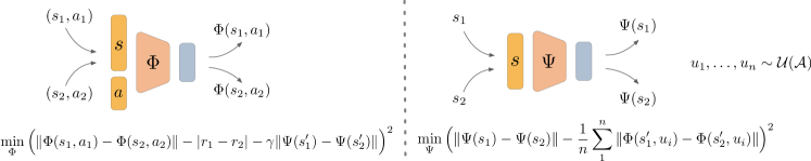
Figure 1: Architecture details of pseudometric learning. Two pairs of Siamese networks $\Phi$ and $\Psi$ are concurrently optimized. Left: the pseudometric $d_{\Phi}$ on $\mathcal{S}\times\mathcal{A}$. Right: The pseudometric $d_{\Psi}$ on $\mathcal{S}$ tracking the boostrapped estimate of $\mathcal{F}(d_{\Phi})$.

We justify this design choice in Section 3.5, where we show that this makes the derivation of the bonus tractable. Therefore, we optimize the two following losses $\hat{\mathcal{L}}_{\Psi}$ and $\hat{\mathcal{L}}_{\Phi}$:

$$\hat{\mathcal{L}}_{\Phi}=\mathop{\mathbb{E}}_{\begin{subarray}{c}s_{1},a_{1},r_{1},s^{\prime}_{1}\sim\mathcal{D}\\ s_{2},a_{2},r_{2},s^{\prime}_{2}\sim\mathcal{D}\end{subarray}}\Big{(}\begin{aligned} &\|\Phi(s_{1},a_{1})-\Phi(s_{2},a_{2})\|\\ &-|r_{1}-r_{2}|-\gamma|\Psi(s^{\prime}_{1})-\Psi(s^{\prime}_{2})|\Big{)}^{2},\end{aligned}$$ (15)

$$\hat{\mathcal{L}}_{\Psi}=\mathop{\mathbb{E}}_{\begin{subarray}{c}s_{1}\sim\mathcal{D},s_{2}\sim\mathcal{D}\end{subarray}}\Big{(}\begin{aligned} &\|\Psi(s_{1})-\Psi(s_{2})\|-\\ &\frac{1}{n}\sum_{\begin{subarray}{c}u_{1},\dots,u_{n}\\ \sim\mathcal{U}(\mathcal{A})\end{subarray}}\|\Phi(s_{1},u_{1})-\Phi(s_{2},u_{2})\|\Big{)}^{2}.\end{aligned}$$ (16)

A visual representation of the two pairs of Siamese networks as well as their losses is provided in Figure 1. Remark that the proposed architecture seems to present similar caveats as naive offline RL approaches (since we estimate quantities that might not be present in the dataset of collected experiences). However, here, the divergence of the quantity at hand (the pseudometric learned) is unlikely since the goal is to minimize a positive quantity. This makes the problem of learning $d_{\Phi}$ inherently more stable than learning an optimal policy. A limitation of this method is that it relies on the reward function $r$ to build similarities between state-action pairs, therefore in very sparse reward environments or with very limited coverage of the state-action space, the quality of the pseudometric learned might conflate state-action pairs together, and hence be less adapted to learn a meaningful measure of similarity.

3.5 Tractable bonus

Once the pseudometric $d_{\Phi}$ is learned, we can define a lookup bonus introduced in section 3.1. Given a monotonously decreasing function $f$, we have: $b(s,a)=f\big{(}\min_{(\hat{s},\hat{a})\in\mathcal{D}}d_{\Phi}(\hat{s},\hat{a};s,a)\big{)}$. This bonus has a complexity that is linear in the size of $\mathcal{D}$ and in the dimension of the representation $\Phi(s,a)$. As we are considering datasets with large numbers of transitions ($\sim 10^{6}$), this makes the exact derivation of the bonus computationally expensive.

Therefore we pre-compute the $k$-nearest neighbors of each state $s\in\mathcal{D}$ according to the Euclidean distance $d_{\Psi}$ induced by $\Psi$; $d_{\Psi}(s_{1},s_{2})=\|\Psi(s_{1})-\Psi(s_{2})\|$. We note:

$$\mathcal{H}(s)=\Big{\{}(\hat{s},\hat{a})\in\mathcal{D}|\;\hat{s}\text{ is a $k$-nearest neighbor of $s$ for $d_{\Psi}$}\Big{\}}.$$ (17)

We infer the approximate distance bonus:

$$\bar{b}(s,a)=f\big{(}\min_{\hat{s},\hat{a}\in\mathcal{H}(s)}d_{\Phi}(s,a;\hat{s},\hat{a})\big{)}.$$ (18)

Pre-computing the $k$-nearest neighbors is expensive (the brute force complexity is quadratic in the size of the dataset, and linear in the dimension of the representation $\Psi$). In our experiments, we use a kd-tree algorithm (Friedman et al., 1977) from scikit-learn (Pedregosa et al., 2011). With multiprocessing ($\sim 50$ CPUs), pre-computing nearest neighbors did not take more than a couple hours even for the largest dataset ($2.10^{6}$ transitions). If the size of the dataset were to be larger, we can naturally scale our method with approximate nearest neighbor methods.

3.6 Algorithm

We now compile the results from this section and present the pseudocode of our method in Algorithms 1 and 2. We refer to the combination of both as PLOff (Pseudometric Learning Offline RL).

1:  Initialize $\Phi$, $\Psi$ networks.

2:  for step $i=1$ to $N$ do

3:     Train $\Phi$: $\min_{\Phi}\hat{\mathcal{L}}_{\Phi}$

4:     Train $\Psi$: $\min_{\Psi}\hat{\mathcal{L}}_{\Psi}$

5:  Initialize $k$-nearest neighbors array $H$.

6:  for step $j=1$ to $|\mathcal{D}|$ do

7:     Compute k-nearest neighbors of $\Psi(s_{j})$.

8:     Add k-nearest neighbors to the array $H$.

Algorithm 1 Bonus learning.

1:  Initialize action-value network $Q_{\omega}$, target network $Q_{\bar{\omega}}$, $Q_{\omega}$ and policy $\pi_{\theta}$.

2:  for step $i=0$ to $K$ do

3:     Train $Q_{\omega}$: $\min_{\omega}\big{(}Q_{\omega}(s,a)-r-Q_{\bar{\omega}}(s^{\prime},\pi_{\theta}(s^{\prime}))-{\color[rgb]{0,0,1}\alpha_{c}\bar{b}(s^{\prime},\pi(s^{\prime}))}\big{)}^{2}$

4:     Train $\pi_{\theta}$: $\max_{\theta}Q_{\omega}(s,\pi_{\theta}(s))+{\color[rgb]{0,0,1}\alpha_{a}\bar{b}(s,\pi(s))}$

5:     Update target network $Q_{\bar{\omega}}:=Q_{\omega}$

Algorithm 2 Actor-Critic Training.

4 Experiments

In this section we conduct an experimental study for the proposed approach. We evaluate it on a series of hand manipulation tasks (Rajeswaran et al., 2018), as well as MuJoCo locomotion tasks (Todorov et al., 2012; Brockman et al., 2016) with multiple data collection strategies from Fu et al. (2020). We first show the details of the learning procedure of the pseudometric, before showing its performance against several baselines from Fu et al. (2020). All implementation details can be found in Appendix B.

4.1 Evaluation environments

We evaluate PLOff on four hand manipulation tasks (Rajeswaran et al., 2018): nailing a hammer, opening a door, manipulating a pen and relocating a ball. We also evaluate PLOff on MuJoCo locomotion tasks (Brockman et al., 2016) where the goal is to maximize the distance traveled: Walker2d, HalfCheetah and Hopper. We provide visualization of the environments in Figure 2. For each environment we consider multiple datasets $\mathcal{D}$ from the D4RL benchmark (Fu et al., 2020). On hand manipulation tasks, these datasets are the following, ”human”: transitions collected by a human operator, ”cloned”: transitions collected by a policy trained with behavioral cloning interacting in the environment + the initial demonstrations, ”expert”: transitions collected by a fine-tuned RL policy interacting in the environment. On locomotion tasks, the datasets are the following, ”random”: transitions collected by a random policy, ”medium-replay” the first 1M transitions collected by a SAC agent (Haarnoja et al., 2018) trained from scratch on the environment, ”medium” transitions collected by a policy with suboptimal performance, ”medium-expert”: transitions collected by a near optimal policy + transitions collected by a suboptimal policy. To have comparable range of rewards between environments, we scale offline rewards by scaling them in $(0,1)$ by $r:=(r-\min_{\mathcal{D}}r)/(\max_{\mathcal{D}}r-\min_{\mathcal{D}}r)$ and learn a policy on this scaled reward.

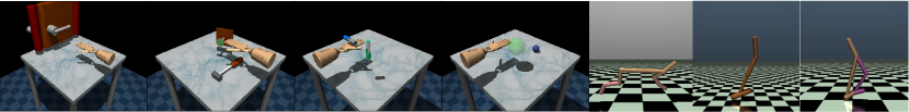
Figure 2: Visualization of the environments considered. From left to right: Door, Hammer, Pen, Relocate, HalfCheetah, Hopper, Walker2d.

4.2 Pseudometric learning

We concurrently learn the deep networks $\Phi$ and $\Psi$ by minimizing the losses $\hat{\mathcal{L}}_{\Phi}$ and $\hat{\mathcal{L}}_{\Psi}$. State-action pairs are concatenated (and states only in the case of $\Psi$) and are passed to a 2-layer network of layers sizes (1024, 32), with a relu activation on top of the first layer. Note that the concatenation step could be preceded by two disjoint layers to which the state and action are passed (thus making it more handy for visual-based obseravations). We sample 256 actions to derive the bootstrapped estimate (loss $\hat{\mathcal{L}}_{\Psi}$). We optimize $\hat{\mathcal{L}}_{\Phi}$ and $\hat{\mathcal{L}}_{\Psi}$ using the Adam optimizer (Kingma & Ba, 2015) with batches of state-action pairs and states of size 256.

To present a qualitative intuition on the nature of the pseudometric learned, we first present the learned pseudometric on a gridworld environment with walls presented in Figure 3. There is a single reward state and we impose a time limit of 50 steps. We gather all transitions visited by the Q-learning algorithm trained for 500 episodes, with $\epsilon$-exploration ($\epsilon=0.1$) and a discount factor $\gamma=0.99$. States and actions are both represented using one-hot encoding. We represent the learned distances (in the sense of $d_{\psi}$) from the central state and from the goal state to the rest of the states. Interestingly, the distance learned takes into account the geometry of the environment, hence showing that it is task relevant. In the left part of the gridworld (far from reward), states tend to be conflated together which highlights the limitation of our work in sparse environments.

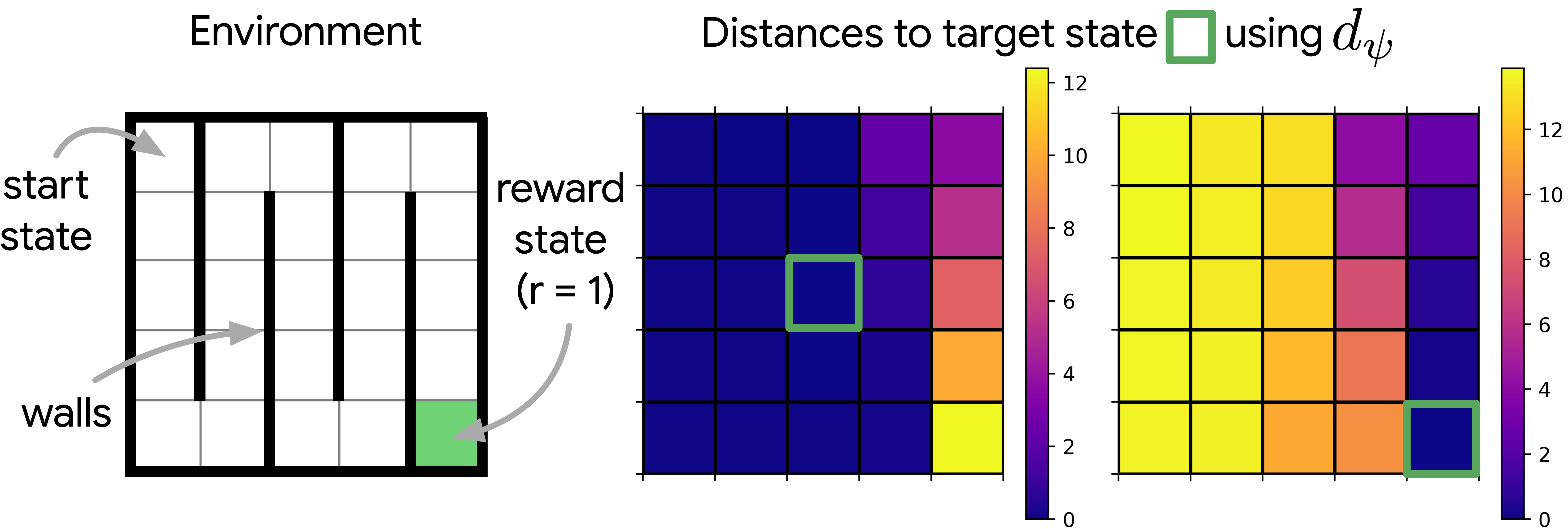
Figure 3: Visualization of the learned pseudometric (center and right) in a gridworld (left). The distance from each state to the ”central” state is represented in the center figure, and to the reward state in the right figure.

For the D4RL environments, we show in Figure 5 the decreasing learning curves for $\hat{\mathcal{L}}_{\Phi}$ and $\hat{\mathcal{L}}_{\Psi}$. In Figure 5, we show that the distribution of the learned distance $d_{\Phi}$ between state-action couples and perturbated versions of themselves (with Gaussian noise either on the state or the action). We show that the distance respects the intuition that the greater the perturbation is, the larger the distance becomes. Finally we provide visualizations of the state similarities learned by $\Psi$ in Appendix C.

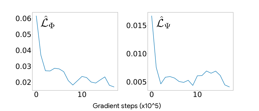
Figure 4: Learning curve of $\Phi$ and $\Psi$, for the Walker2d environment together with the ”medium-replay” dataset from Fu et al. (2020). We show the values (averaged over batch) of $\hat{\mathcal{L}}_{\Phi}$ (left) and $\hat{\mathcal{L}}_{\Psi}$ (right) throughout the learning procedure.

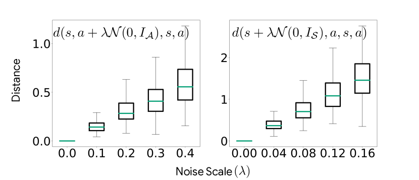
Figure 5: Influence of noise on the distance. We show on the left the learned distance of a state-action pair $(s,a)$ to a perturbated version of itself $(s,a+\lambda\mathcal{N}(0,I_{\mathcal{A}})$. We show on the right the learned distance of a state-action pair $(s,a)$ to a perturbated version of itself $(s+\lambda\mathcal{N}(0,I_{\mathcal{S}}),a)$.

4.3 Agent training with pseudometric bonus

In this section, we empirically evaluate the performance of an agent trained with a bonus based on the pseudometric. In our experiments, we use TD3 (Fujimoto et al., 2019). It is an off-policy actor-critic algorithm (Konda & Tsitsiklis, 2000) which builds on top of DDPG (Lillicrap et al., 2016). We use an implementation of TD3 where we load the dataset of experiences $\mathcal{D}$ in its replay buffer. We concurrently learn a policy $\pi_{\theta}$ and an action-value function $Q_{\omega}$. The critic loss and actor loss are modified to incorporate the pseudometric bonus, as described in Algorithm 2.

We found that the bonus defined as $\bar{b}(s,a):=Q_{\bar{\omega}}(s,a)\exp(-\beta d_{\mathcal{D}}(s,a))$ leads to strong empirical results. This bonus form is quite natural, since it uses the action-value function to scale the value of the bonus (and therefore enables hyperparameters to be more robust).

We ran a hyperparameter search on $\alpha_{a},\alpha_{c}\in\{1,5,10\}$ and $\beta\in\{0.1,0.25,0.5\}$. We select the best hyperparameters for each family of environments (locomotion and hand manipulation), and re-run for 10 seeds. For each seed we evaluate the resulting policy on 10 episodes. We report performance in Table 1. We compare the method with numerous baselines: AWR (Peng et al., 2019), Behavioral Cloning (Pomerleau, 1991), BEAR (Kumar et al., 2019), BRAC (Wu et al., 2019), BCQ (Fujimoto et al., 2018) and CQL (Kumar et al., 2020).

Algorithm	BC	BEAR	BRAC-v	AWR	BCQ	CQL	PLOff	PLOff-L2	TD3-Off
cheetah-rand	2.1	25.1	31.2	2.5	2.2	35.4	1.7 $\pm$ 0.1	2.2 $\pm$ 0.0	28.0 $\pm$ 2.6
walker-rand	1.6	7.3	1.9	1.5	4.9	7.0	0.7 $\pm$ 1.1	4.7 $\pm$ 7.3	1.1 $\pm$ 1.2
hopper-rand	9.8	11.4	12.2	10.2	10.6	10.8	11.5 $\pm$ 0.1	11.6 $\pm$ 0.2	0.9 $\pm$ 0.4
cheetah-med	36.1	41.7	46.3	37.4	40.7	44.4	38.2 $\pm$ 0.4	38.0 $\pm$ 0.4	0.3 $\pm$ 4.4
walker-med	6.6	59.1	81.1	17.4	53.1	79.2	73.2 $\pm$ 7.4	72.2 $\pm$ 3.4	0.0 $\pm$ 0.3
hopper-med	29.0	52.1	31.1	35.9	54.5	58.0	87.0 $\pm$ 18.2	76.7 $\pm$ 10.3	0.9 $\pm$ 0.5
cheetah-med-rep	38.4	38.6	47.7	40.3	38.2	46.2	38.5 $\pm$ 1.6	39.0 $\pm$ 1.3	35.9 $\pm$ 3.6
walker-med-rep	11.3	19.2	0.9	15.5	15.0	26.7	23.2 $\pm$ 9.3	14.6 $\pm$ 6.9	8.0 $\pm$ 4.3
hopper-med-rep	11.8	33.7	0.6	28.4	33.1	48.6	33.5 $\pm$ 10.1	48.2 $\pm$ 11.5	9.9 $\pm$ 9.4
cheetah-med-exp	35.8	53.4	41.9	52.7	64.7	62.4	58.0 $\pm$ 8.2	52.1 $\pm$ 8.8	3.4 $\pm$ 1.9
walker-med-exp	6.4	40.1	81.6	53.8	57.5	111.0	98.8 $\pm$ 8.2	98.5 $\pm$ 8.5	0.4 $\pm$ 1.5
hopper-med-exp	111.9	96.3	0.8	27.1	110.9	98.7	112.1 $\pm$ 0.3	107.6 $\pm$ 10.0	5.5 $\pm$ 5.4
Mean perf	25.0	39.8	31.4	26.8	40.4	52.3	48.0 $\pm$ 5.4	47.0 $\pm$ 5.7	7.3 $\pm$ 3.0
pen-human	34.4	-1.0	0.6	12.3	68.9	37.5	69.6 $\pm$ 22.0	69.9 $\pm$ 14.2	0.0 $\pm$ 4.0
hammer-human	1.5	0.3	0.2	1.2	0.5	4.4	2.5 $\pm$ 1.6	1.7 $\pm$ 1.2	0.2 $\pm$ 0.0
door-human	0.5	-0.3	-0.3	0.4	-0.0	9.9	-0.2 $\pm$ 0.2	0.6 $\pm$ 1.6	-0.3 $\pm$ 0.0
relocate-human	0.0	-0.3	-0.3	-0.0	-0.1	0.2	0.0 $\pm$ 0.0	0.0 $\pm$ 0.1	-0.3 $\pm$ 0.0
pen-cloned	56.9	26.5	-2.5	28.0	44.0	39.2	35.4 $\pm$ 7.7	31.7 $\pm$ 10.1	-3.7 $\pm$ 0.5
hammer-cloned	0.8	0.3	0.3	0.4	0.4	2.1	0.4 $\pm$ 0.0	0.4 $\pm$ 0.1	0.2 $\pm$ 0.0
door-cloned	-0.1	-0.1	-0.1	0.0	0.0	0.4	0.0 $\pm$ 0.0	0.0 $\pm$ 0.0	-0.2 $\pm$ 0.1
relocate-cloned	-0.1	-0.3	-0.3	-0.2	-0.3	-0.1	-0.2 $\pm$ 0.0	-0.2 $\pm$ 0.0	-0.2 $\pm$ 0.0
pen-expert	85.1	105.9	-3.0	111.0	114.9	107.0	104.8 $\pm$ 22.8	111.8 $\pm$ 12.0	-2.8 $\pm$ 1.2
hammer-expert	125.6	127.3	0.3	39.0	107.2	86.7	116.6 $\pm$ 9.4	120.0 $\pm$ 5.8	0.2 $\pm$ 0.0
door-expert	34.9	103.4	-0.3	102.9	99.0	101.5	104.2 $\pm$ 2.0	104.0 $\pm$ 1.4	-0.1 $\pm$ 0.1
relocate-expert	101.3	98.6	-0.4	91.5	41.6	95.0	107.0 $\pm$ 2.4	77.3 $\pm$ 1.4	-0.3 $\pm$ 0.0
Mean perf	36.7	38.3	-0.4	32.2	39.6	40.3	45.0 $\pm$ 5.7	43.2 $\pm$ 4.3	-0.6 $\pm$ 0.5

Table 1: Evaluation of PLOff. We report the results of the baselines using performance results reported by Fu et al. (2020), which do not incorporate standard deviation of performances, since the numbers are based on 3 seeds. In our case we use 10 seeds, following recommendations from Henderson et al. (2018), and evaluate on 10 episodes for each seed before reporting average and standard deviations of performance. Results are bolded if they are best on average, underlined if within a standard deviation of the best average performance.

Table 1 shows the performance of PLOff on the D4RL benchmark. On average, it tops other methods on hand manipulation tasks, and tops all methods but CQL on locomotion tasks. However, even if PLOff performs well across the board, the approach does not solve the common failure cases shared by all methods (random datasets as well as datasets with human operated transitions, see Table 1).

4.4 Ablations

We perform two ablations of the proposed method and report results in Table 1. The first one consists in using TD3 without any bonus that we note TD3-off. The second one is similar to PLOff although with a bonus based on the Euclidean distance between the concatenation of the state and the action rather than a learned distance, we refer to it as PLOff-L2. For PLOff-L2, we used the same experimental evaluation protocol and hyperparameter search as the proposed method.

The results in Table 1 show that without a bonus, the performance of the policy learned is mediocre. On the other hand, PLOff-L2 reaches performance slightly below PLOff. This should not come as a surprise since the Euclidean distance has been shown to be an effective measure of similarity in some continuous control tasks (Dadashi et al., 2021). Note however that in more complex tasks (typically vision-based environments), the Euclidean distance is a poor measure of similarity which makes the learning of a pseudometric necessary.

5 Related Work

Offline Reinforcement Learning. Offline RL (Lagoudakis & Parr, 2003; Ernst et al., 2005; Riedmiller, 2005; Pietquin et al., 2011; Lange et al., ; Levine et al., 2020) methods suffer from overestimation of state-action pairs that are not in the support of logged transitions. A number of methods have been explored to mitigate this phenomenon, by constraining the learned policy to be close in terms of a probabilistic distance to the behavioral policy (Jaques et al., 2019; Wu et al., 2019; Kumar et al., 2019; Siegel et al., 2020; Peng et al., 2019; Fujimoto et al., 2018), or a pessimistic (Buckman et al., 2021) estimate of either the Q-value or the bootstrapped Q-value (Kumar et al., 2020; Laroche et al., 2019; Simão et al., 2020; Nadjahi et al., 2019). Fujimoto et al. (2018); Kumar et al. (2019); Wu et al. (2019) estimate the behavior policy using a conditional VAE (Kingma & Welling, 2014), and constrain the policy learned offline with a distance to the behavior policy using the Kullback-Leibler divergence, the Wasserstein distance and the Maximum-Mean Discrepancy respectively.

In this work we trade the problem of estimating the behavioral policy (which is specially problematic if it is multimodal) with the computational cost of a lookup; and instead of penalizing the policy with a distribution-based distance, we learn a task relevant pseudometric instead. As our bonus is based on learned structural properties of the MDP we can also draw a connection to model-based off-policy RL (Kidambi et al., 2020; Yu et al., 2020; Argenson & Dulac-Arnold, 2021).

State-action similarity in MDPs. Bisimulation relations are a form of state abstraction (Li et al., 2006), introduced in the context of MDPs by Givan et al. (2003), where states with the same rewards and transitions are aggregated. As this definition is strict, a number of works define approximate versions of it. For example, Dean & Givan (1997) use a bound rather than an exact equivalence. Similarly, Ferns et al. (2004) introduce bisimulation metrics (Ferns et al., 2011, 2006), which use the reward signal to decide the proximity between two states. This makes bisimulation metrics close to the difference between optimal values between two states (Ferns & Precup, 2014). Learning a bisimulation metric online (Castro, 2020; Comanici et al., 2012) has been shown to be beneficial to learn controllable representations that eliminates unnecessary details of the state (Zhang et al., 2021) or can be used as an auxiliary loss which leads to improvement performance on the Atari benchmark (Gelada et al., 2019). Castro (2020) introduces the Siamese network architecture, as well as a loss, to derive the bisimulation metric online. Our work differs as it learns a pseudometric on state-action pairs rather than states, and is based on offline transitions.

Ravindran & Barto (2003) introduces MDP homomorphism as another form of abstraction which is state-action dependent rather than state dependent. Again as the partitioning induced by a homomorphism is too restrictive to be useful in practice, a number of work has looked into relaxed versions (Ravindran & Barto, 2004; Wolfe & Barto, 2006; van der Pol et al., 2020; Taylor et al., 2008). Our work is closer to bisimulation metrics since it introduces the similarity between states-actions as a difference between reward accumulated when following the same sequence of actions (except for the first one).

6 Concluding Remarks

We introduced a new paradigm to compute a pseudometric-based bonus for offline RL. We learn policies consistent with the behavior policy that generated the collected transitions, and hence reduce action extrapolation error.

We showed how to derive a pseudometric from logged transitions, extending existing work from Castro (2020) from the online to the offline setting and from pseudometrics on state space to pseudometrics on state-action space. We showed that the pseudometric we desire to learn is the fixed point of an operator, and we provide a neural architecture as well as a loss to learn it.

Conceptually, our bonus introduces a larger computational cost against other approaches that reduce extrapolation errors. We argue that this is actually a desirable direction of research for offline RL. In the presence of a fixed dataset of transitions, and since we cannot add new transitions into memory, we should insist on the other side of the well-known memory-computation trade-off.

We demonstrated in our experimental study that our method performs comparably to existing state-of-the-art methods (tops other methods on hand manipulation task, second to top on locomotion tasks).

Appendix

Appendix A Proofs

See 3.1

Proof.

Let $d$ be a pseudometric in $\mathbb{M}$, we show that $\mathcal{F}(d)$ respects all properties in Definition 1 and therefore is a pseudometric. Let $(s_{1},a_{1}),(s_{2},a_{2}),(s_{3},a_{3})\in\mathcal{S}\times\mathcal{A}$ and their associated rewards $r_{1},r_{2},r_{3}$ and next states $s^{\prime}_{1},s^{\prime}_{2},s^{\prime}_{3}$:

• the pseudo-distance of a couple to itself is null:

  $$\mathcal{F}(d)(s_{1},a_{1};s_{1},a_{1}) =\underbrace{|r_{1}-r_{1}|}_{=0}+\gamma\mathop{\mathbb{E}}_{u\in\mathcal{U}(\mathcal{A})}\underbrace{d(s^{\prime}_{1},u;s^{\prime}_{1},u)}_{=0\;\text{since $d$ is a pseudometric}}=0;$$

• symmetry:

  $$\mathcal{F}(d)(s_{1},a_{1};s_{2},a_{2}) =\underbrace{|r_{1}-r_{2}|}_{=|r_{2}-r_{1}|}+\gamma\mathop{\mathbb{E}}_{u\in\mathcal{U}(\mathcal{A})}\underbrace{d(s^{\prime}_{1},u;s^{\prime}_{2},u)}_{=d(s^{\prime}_{2},u;s^{\prime}_{1},u)\;\text{since $d$ is a pseudometric}}=\mathcal{F}(d)(s_{2},a_{2};s_{1},a_{1});$$

• triangular inequality:

  $$\mathcal{F}(d)(s_{1},a_{1};s_{3},a_{3}) =|r_{1}-r_{3}|+\gamma\mathop{\mathbb{E}}_{u\in\mathcal{U}(\mathcal{A})}d(s^{\prime}_{1},u;s^{\prime}_{3},u)$$

  $$\leq|r_{1}-r_{2}|+|r_{2}-r_{3}|+\gamma\mathop{\mathbb{E}}_{u\in\mathcal{U}(\mathcal{A})}d(s^{\prime}_{1},u;s^{\prime}_{2},u)+d(s^{\prime}_{2},u;s^{\prime}_{3},u)$$

  $$\leq\mathcal{F}(d)(s_{1},a_{1};s_{2},a_{2})+\mathcal{F}(d)(s_{2},a_{2};s_{3},a_{3}).$$

∎

See 3.2

Proof.

Let $d_{1},d_{2}\in\mathbb{M}$, let $(s_{1},a_{1}),(s_{2},a_{2})\in\mathcal{S}\times\mathcal{A}$ and their associated rewards $r_{1},r_{2}$ and next states $s^{\prime}_{1},s^{\prime}_{2}$, we have:

$$\mathcal{F}(d_{1})(s_{1},a_{1};s_{2},a_{2}) -\mathcal{F}(d_{2})(s_{1},a_{1};s_{2},a_{2})$$

$$=|r_{1}-r_{2}|-|r_{1}-r_{2}|+\gamma\mathop{\mathbb{E}}_{u\in\mathcal{U}(\mathcal{A})}d_{1}(s^{\prime}_{1},u;s^{\prime}_{2},u)-\gamma\mathop{\mathbb{E}}_{u\in\mathcal{U}(\mathcal{A})}d_{2}(s^{\prime}_{1},u;s^{\prime}_{2},u)$$

$$=\gamma\mathop{\mathbb{E}}_{u\in\mathcal{U}(\mathcal{A})}d_{1}(s^{\prime}_{1},u;s^{\prime}_{2},u)-d_{2}(s^{\prime}_{1},u;s^{\prime}_{2},u).$$

Therefore, we have:

$$|\mathcal{F}(d_{1})(s_{1},a_{1};s_{2},a_{2})-\mathcal{F}(d_{2})(s_{1},a_{1};s_{2},a_{2})| \leq\gamma\mathop{\mathbb{E}}_{u\in\mathcal{U}(\mathcal{A})}|d_{1}(s^{\prime}_{1},u;s^{\prime}_{2},u)-d_{2}(s^{\prime}_{1},u;s^{\prime}_{2},u)|$$

$$\leq\gamma\max_{u\in\mathcal{A}}|d_{1}(s^{\prime}_{1},u;s^{\prime}_{2},u)-d_{2}(s^{\prime}_{1},u;s^{\prime}_{2},u)|$$

$$\leq\gamma\max_{s,s^{\prime}\in\mathcal{S}}\max_{u,u^{\prime}\in\mathcal{A}}|d_{1}(s,u;s^{\prime},u^{\prime})-d_{2}(s,u;s^{\prime},u^{\prime})|$$

$$\leq\gamma\|d_{1}-d_{2}\|_{\infty}.$$

We thus have that $\|\mathcal{F}(d_{1})-\mathcal{F}(d_{2})\|_{\infty}\leq\gamma\|d_{1}-d_{2}\|_{\infty}$, therefore $\mathcal{F}$ is a $\gamma$-contraction for $\|\cdot\|_{\infty}$. ∎

See 3.3

Proof.

This is a direct application of the Banach theorem (Banach, 1922). $\mathcal{F}$ is a $\gamma$-contracting operator with $\gamma\in[0,1)$, in the metric space $((\mathcal{S}\times\mathcal{A})\times(\mathcal{S}\times\mathcal{A}),\|\cdot\|_{\infty})$, therefore using the Banach theorem we have that $\mathcal{F}$ has a unique fixed point $d^{*}$ and $\forall d_{0}\in\mathbb{M},\lim_{n\to\infty}\mathcal{F}^{n}(d_{0})=d^{*}$. ∎

See 3.4

Proof.

The repeated application of $\hat{\mathcal{F}}$ is an asynchronous fixed point iteration scheme. The convergence to $d^{*}$ (almost surely) is a direct application of Proposition 3 from Bertsekas & Tsitsiklis (1991). Note that the state-action coverage assumption enables to apply this result since all pairs of state-action are visited an infinite number of times (almost surely).

∎

Appendix B Implementation

In this section, we provide a detailed description of the experimental study.

Offline datasets preprocessing.

We use datasets from Fu et al. (2020). We scale the rewards by shifting them by $-\min_{r\sim\mathcal{D}}r$ and dividing them by $\max_{r\sim\mathcal{D}}r-\min_{r\sim\mathcal{D}}r$ for both pseudometric learning and policy learning. This enables to have comparable range of rewards between environments.

Pseudometric learning.

The Siamese networks $\Phi$ et $\Psi$ have the same architecture: a two-layer MLP of size $(1024,32)$ with relu activation on top of the first layer. Note that $\Phi$ takes the concatenation of state and action as input, whereas $\Psi$ only takes the state as an input. We use a discount factor $\gamma=0.9$ (which is different than the discount factor from the agent) in the experiments (we noticed some instabilities on human datasets, which contains less transitions than the rest of the datasets, if the discount factor is larger).

We minimize the losses $\hat{\mathcal{L}}_{\Phi}$ and $\hat{\mathcal{L}}_{\Psi}$ using the Adam optimizer with a learning rate $10^{-3}$. The batch size used to compute the losses is $256$. The bootstrapped estimate in $\hat{\mathcal{L}}_{\Phi}$ is estimated with $256$ actions sampled uniformly. We train the two networks by iteratively taking a gradient step on each loss for $2.10^{6}$ gradient steps with parameters updated using exponential parameters averaging with a rate $\tau=0.005$

Once the $\Psi$ network is trained, we derive the $k$-nearest neighbors of each state in $\mathcal{D}$ for the distance induced by $\Psi$, with $k=50$. The nearest neighbors are computed using the scikit-learn implementation of the kd-tree algorithm, taking advantage of multiprocessing (with 50 CPUs).

Agent training.

We re-implemented the TD3 agent from Fujimoto et al. (2019) in jax (Bradbury et al., 2018). We use the default hyperparameters (and did not perform HP search).

For the critic, we used a three-layer network with size $(256,256,1)$ with tanh activation on top of the first layer and elu activation on top of the second layer. For the policy, we used a three-layer network with size $(256,256,|\mathcal{A}|)$ where $|\mathcal{A}|$ is the dimension of the action space, with tanh activation on top of the first layer, elu activation on top of the second layer and tanh activation on top of the last layer. We used the Adam optimizer for both the actor and the critic and used a learning rate of $3.10^{-4}$ (consistently with Fujimoto et al. (2019)) and trained them using batch of transitions of size 256 sampled uniformly in $\mathcal{D}$, for 500000 gradient steps.

We led experiments with the following bonuses $\bar{b}$ (and focused on the first one as it led to better empirical performance):

• $\bar{b}(s,a)=Q_{\bar{\omega}}(s,a)\exp(-\beta d_{\mathcal{D}}(s,a))$

• $\bar{b}(s,a)=\exp(-\beta d_{\mathcal{D}}(s,a))$

• $\bar{b}(s,a)=1-\exp(\beta d_{\mathcal{D}}(s,a))$

We led a hyperparameter search for both the locomotion environments and the hand manipulation environments on $\alpha_{a},\alpha_{c},\beta$. We selected $\alpha_{a},\alpha_{c}$ in $\{1,5,10\}$, $\beta\in\{0.1,0.25,0.5\}$ as the better combination on the average normalized performance on the tasks (averaged over 3 seeds). We re-ran the best combination of hyperparameters for 10 seeds and report results averaged over the 10 seeds and 10 evaluation episodes per seed. We found that the best combination for hand manipulation tasks was $\alpha_{a}=10,\alpha_{c}=10,\beta=0.5$ and for locomotion tasks was $\alpha_{a}=5,\alpha_{c}=1,\beta=0.5$.

Appendix C Metric Visualization

In this section, we show the state similarity learned by PLOff ($\Psi$ network) and visualize it for MuJoCo locomotion environments (we could not provide such visualizations on Adroit tasks since states cannot be retrieved from observations, which is the necessary condition to generate rendering).

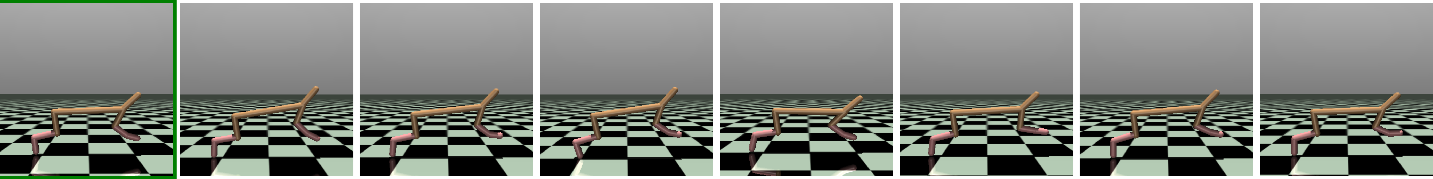
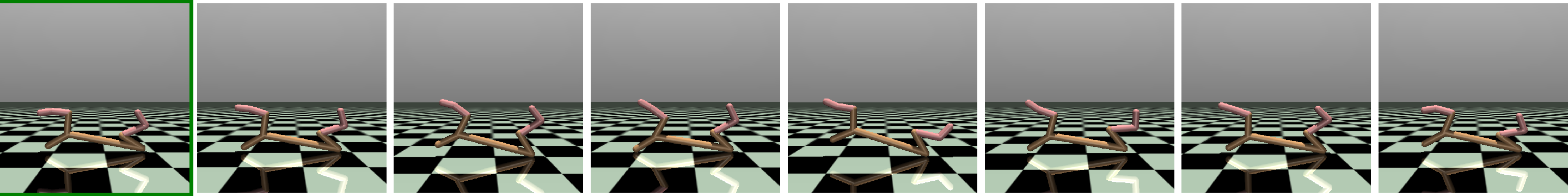
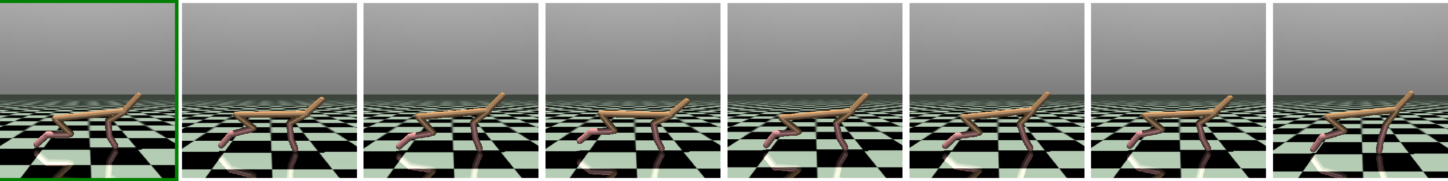
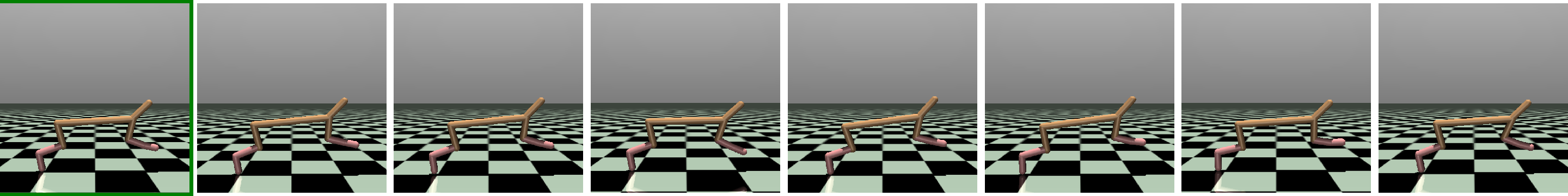
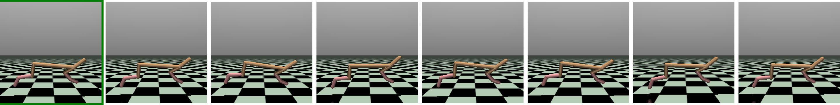
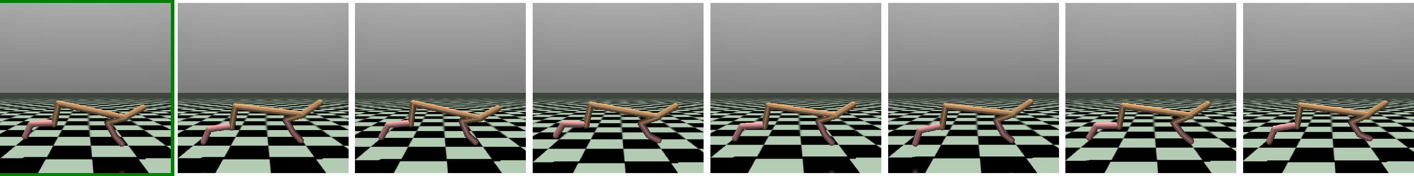
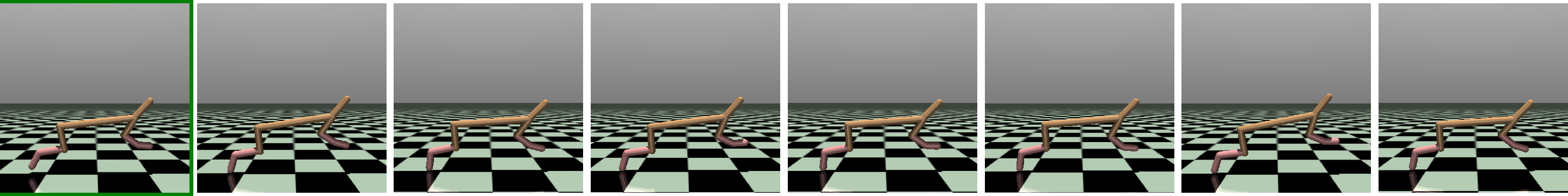
Figure 6: State similarity learned by PLOff for HalfCheetah on the medium-replay dataset. For each row, the leftmost image is the state for which we compute nearest neighbors in the dataset $\mathcal{D}$ for the metric induced by $\Psi$ (ranked by decreasing level of similarity).

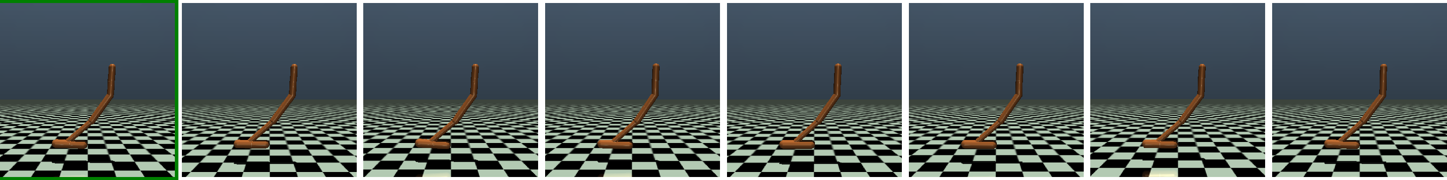
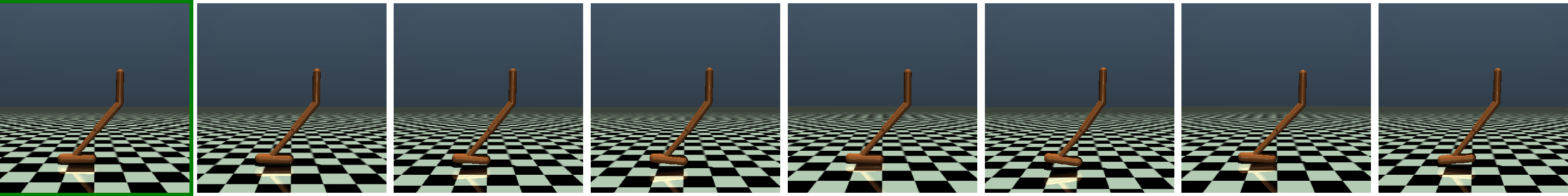
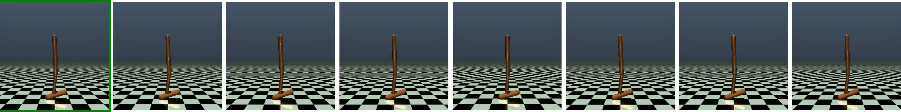
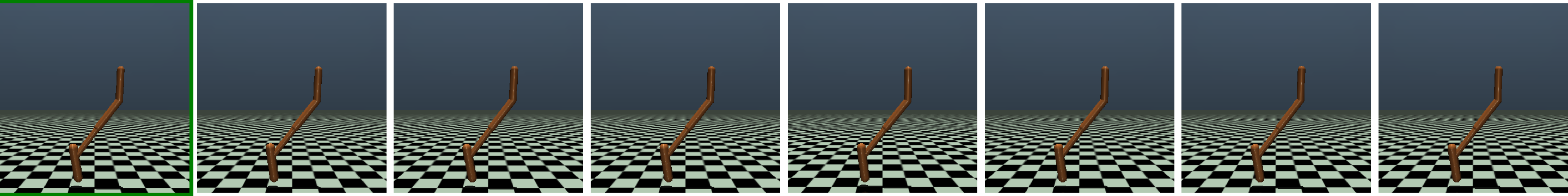
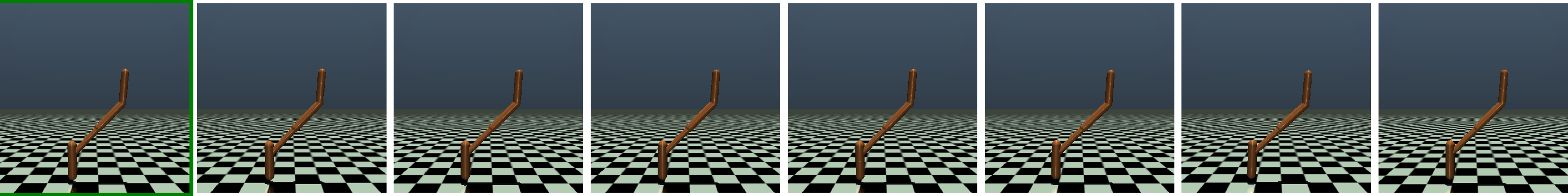
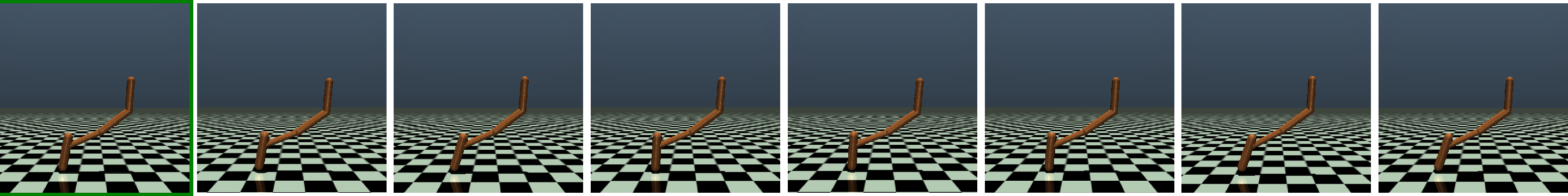
Figure 7: State similarity learned by PLOff for Hopper on the medium-replay dataset. For each row, the leftmost image is the state for which we compute nearest neighbors in the dataset $\mathcal{D}$ for the metric induced by $\Psi$ (ranked by decreasing level of similarity).

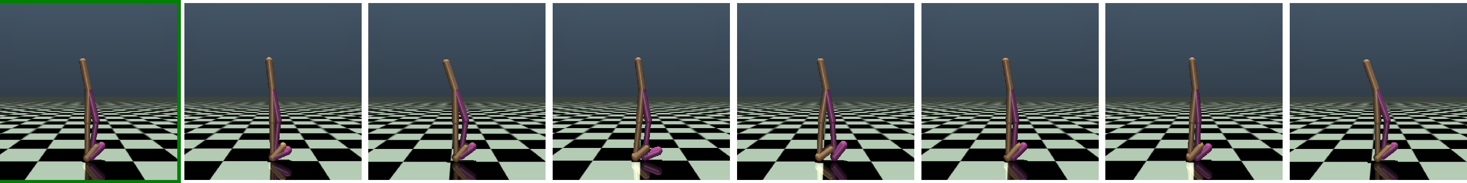
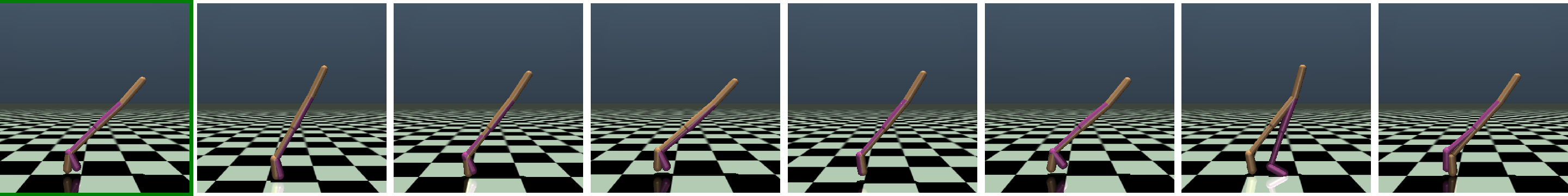
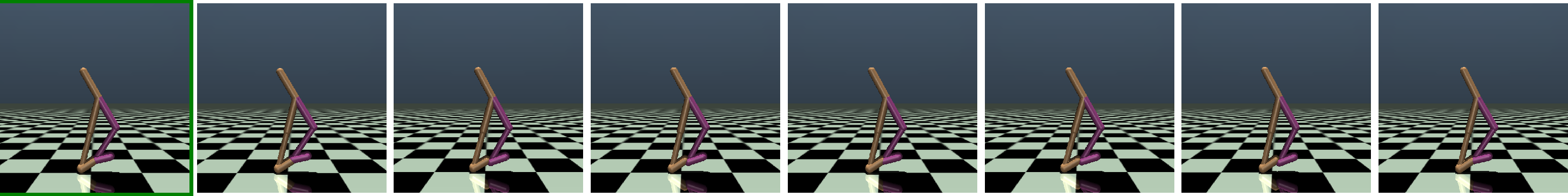
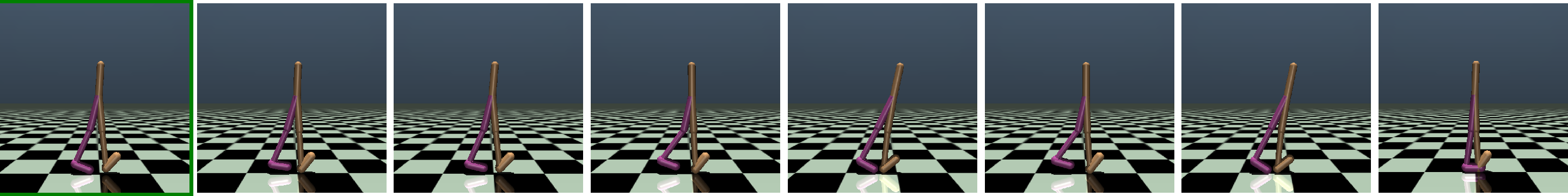
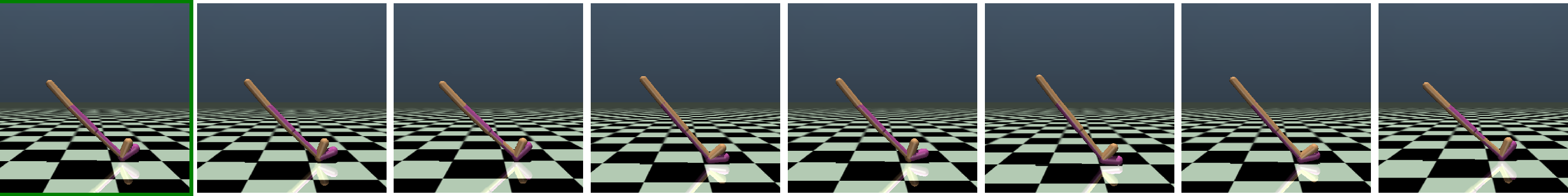
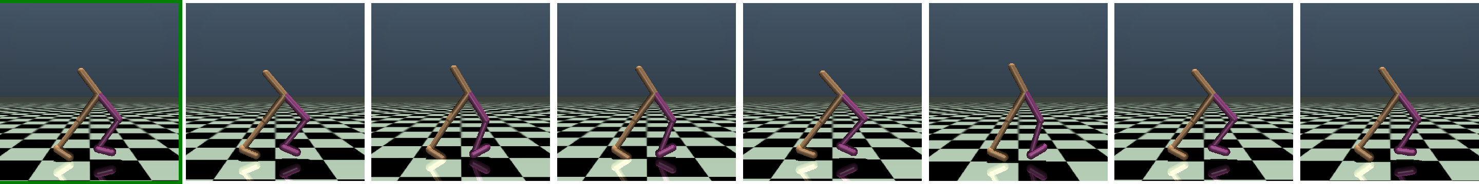
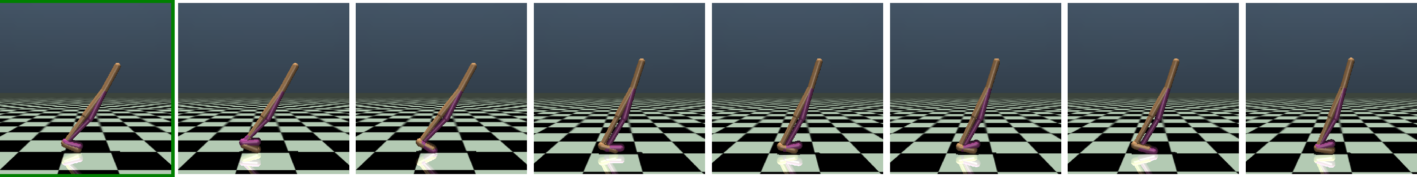
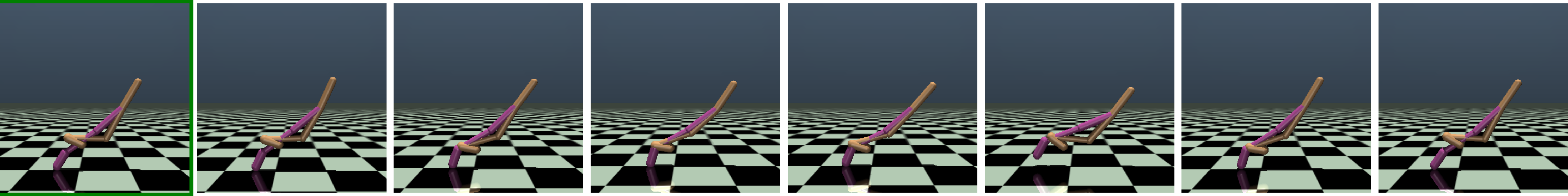
Figure 8: State similarity learned by PLOff for Walker2d on the medium-replay dataset. For each row, the leftmost image is the state for which we compute nearest neighbors in the dataset $\mathcal{D}$ for the metric induced by $\Psi$ (ranked by decreasing level of similarity).

References

- Argenson & Dulac-Arnold (2021) Argenson, A. and Dulac-Arnold, G. Model-based offline planning. International Conference on Learning Representations (ICLR), 2021.
- Banach (1922) Banach, S. Sur les opérations dans les ensembles abstraits et leur application aux équations intégrales. Fund. math, 1922.
- Bellemare et al. (2016) Bellemare, M. G., Srinivasan, S., Ostrovski, G., Schaul, T., Saxton, D., and Munos, R. Unifying count-based exploration and intrinsic motivation. In Neural Information Processing Systems (NeurIPS), 2016.
- Bellman (1957) Bellman, R. A markovian decision process. Indiana University Mathematics Journal, 1957.
- Bertsekas & Tsitsiklis (1996) Bertsekas, D. and Tsitsiklis, J. Neuro-dynamic programming. 1996.
- Bertsekas & Tsitsiklis (1991) Bertsekas, D. P. and Tsitsiklis, J. N. Some aspects of parallel and distributed iterative algorithms-a survey. Automatica, 1991.
- Bradbury et al. (2018) Bradbury, J., Frostig, R., Hawkins, P., Johnson, M. J., Leary, C., Maclaurin, D., Necula, G., Paszke, A., VanderPlas, J., Wanderman-Milne, S., and Zhang, Q. JAX: composable transformations of Python+NumPy programs, 2018. URL http://github.com/google/jax.
- Brockman et al. (2016) Brockman, G., Cheung, V., Pettersson, L., Schneider, J., Schulman, J., Tang, J., and Zaremba, W. Openai gym. arXiv preprint arXiv:1606.01540, 2016.
- Bromley et al. (1994) Bromley, J., Guyon, I., LeCun, Y., Säckinger, E., and Shah, R. Signature verification using a” siamese” time delay neural network. Neural Information Processing Systems (NeurIPS), 1994.
- Buckman et al. (2021) Buckman, J., Gelada, C., and Bellemare, M. G. The importance of pessimism in fixed-dataset policy optimization. International Conference on Learning Representations (ICLR), 2021.
- Castro (2020) Castro, P. S. Scalable methods for computing state similarity in deterministic markov decision processes. In AAAI Conference on Artificial Intelligence, 2020.
- Comanici et al. (2012) Comanici, G., Panangaden, P., and Precup, D. On-the-fly algorithms for bisimulation metrics. In International Conference on Quantitative Evaluation of Systems, 2012.
- Dadashi et al. (2021) Dadashi, R., Hussenot, L., Geist, M., and Pietquin, O. Primal wasserstein imitation learning. International Conference on Learning Representations (ICLR), 2021.
- Dean & Givan (1997) Dean, T. and Givan, R. Model minimization in markov decision processes. In AAAI Conference on Artificial Intelligence, 1997.
- Dulac-Arnold et al. (2019) Dulac-Arnold, G., Mankowitz, D. J., and Hester, T. Challenges of real-world reinforcement learning. CoRR, abs/1904.12901, 2019.
- Ernst et al. (2005) Ernst, D., Geurts, P., and Wehenkel, L. Tree-based batch mode reinforcement learning. Journal of Machine Learning Research, 2005.
- Ferns & Precup (2014) Ferns, N. and Precup, D. Bisimulation metrics are optimal value functions. In Uncertainty in Artificial Intelligence (UAI), 2014.
- Ferns et al. (2004) Ferns, N., Panangaden, P., and Precup, D. Metrics for finite markov decision processes. In Uncertainty in Artificial Intelligence (UAI), 2004.
- Ferns et al. (2006) Ferns, N., Castro, P. S., Precup, D., and Panangaden, P. Methods for computing state similarity in markov decision processes. Uncertainty in Artificial Intelligence (UAI), 2006.
- Ferns et al. (2011) Ferns, N., Panangaden, P., and Precup, D. Bisimulation metrics for continuous markov decision processes. SIAM Journal on Computing, 2011.
- Friedman et al. (1977) Friedman, J., Bentley, J., and Finkel, R. An algorithm for finding best matches in logarithmic expected time. ACM Trans. Math. Softw., 1977.
- Fu et al. (2020) Fu, J., Kumar, A., Nachum, O., Tucker, G., and Levine, S. D4rl: Datasets for deep data-driven reinforcement learning. arXiv preprint arXiv:2004.07219, 2020.
- Fujimoto et al. (2018) Fujimoto, S., van Hoof, H., and Meger, D. Addressing function approximation error in actor-critic methods. In International Conference on Machine Learning (ICML), 2018.
- Fujimoto et al. (2019) Fujimoto, S., Meger, D., and Precup, D. Off-policy deep reinforcement learning without exploration. In International Conference on Machine Learning (ICML), 2019.
- Gelada et al. (2019) Gelada, C., Kumar, S., Buckman, J., Nachum, O., and Bellemare, M. G. Deepmdp: Learning continuous latent space models for representation learning. In International Conference on Machine Learning (ICML), 2019.
- Givan et al. (2003) Givan, R., Dean, T., and Greig, M. Equivalence notions and model minimization in markov decision processes. Artificial Intelligence, 2003.
- Haarnoja et al. (2018) Haarnoja, T., Zhou, A., Abbeel, P., and Levine, S. Soft actor-critic: Off-policy maximum entropy deep reinforcement learning with a stochastic actor. In International Conference on Machine Learning (ICML), 2018.
- Henderson et al. (2018) Henderson, P., Islam, R., Bachman, P., Pineau, J., Precup, D., and Meger, D. Deep reinforcement learning that matters. AAAI Conference on Artificial Intelligence, 2018.
- Jaques et al. (2019) Jaques, N., Ghandeharioun, A., Shen, J. H., Ferguson, C., Lapedriza, A., Jones, N., Gu, S., and Picard, R. Way off-policy batch deep reinforcement learning of implicit human preferences in dialog. arXiv preprint arXiv:1907.00456, 2019.
- Kidambi et al. (2020) Kidambi, R., Rajeswaran, A., Netrapalli, P., and Joachims, T. Morel: Model-based offline reinforcement learning. Neural Information Processing Systems (NeurIPS), 2020.
- Kim & Park (2018) Kim, K.-E. and Park, H. Imitation learning via kernel mean embedding. In AAAI Conference on Artificial Intelligence, 2018.
- Kingma & Ba (2015) Kingma, D. P. and Ba, J. Adam: A method for stochastic optimization. In International Conference on Learning Representations (ICLR), 2015.
- Kingma & Welling (2014) Kingma, D. P. and Welling, M. Auto-encoding variational bayes. CoRR, abs/1312.6114, 2014.
- Konda & Tsitsiklis (2000) Konda, V. and Tsitsiklis, J. Actor-critic algorithms. In Neural Information Processing Systems (NeurIPS), 2000.
- Kumar et al. (2019) Kumar, A., Fu, J., Tucker, G., and Levine, S. Stabilizing off-policy q-learning via bootstrapping error reduction. Neural Information Processing Systems (NeurIPS), 2019.
- Kumar et al. (2020) Kumar, A., Zhou, A., Tucker, G., and Levine, S. Conservative q-learning for offline reinforcement learning. Neural Information Processing Systems (NeurIPS), 2020.
- Lagoudakis & Parr (2003) Lagoudakis, M. G. and Parr, R. Least-squares policy iteration. Journal of Machine Learning Research, 2003.
- (38) Lange, S., Gabel, T., and Riedmiller, M. Batch reinforcement learning. In Reinforcement learning.
- Laroche et al. (2019) Laroche, R., Trichelair, P., and Des Combes, R. T. Safe policy improvement with baseline bootstrapping. In International Conference on Machine Learning (ICML), 2019.
- Le Lan et al. (2021) Le Lan, C., Bellemare, M. G., and Castro, P. S. Metrics and continuity in reinforcement learning. AAAI Conference on Artificial Intelligence, 2021.
- Levine et al. (2020) Levine, S., Kumar, A., Tucker, G., and Fu, J. Offline reinforcement learning: Tutorial, review, and perspectives on open problems. arXiv preprint arXiv:2005.01643, 2020.
- Li et al. (2006) Li, L., Walsh, T. J., and Littman, M. L. Towards a unified theory of state abstraction for mdps. International Symposium on Artificial Intelligence and Mathematics (ISAIM), 2006.
- Lillicrap et al. (2016) Lillicrap, T. P., Hunt, J. J., Pritzel, A., Heess, N., Erez, T., Tassa, Y., Silver, D., and Wierstra, D. Continuous control with deep reinforcement learning. In International Conference on Learning Representations (ICLR), 2016.
- Lin (1992) Lin, L. J. Self-improving reactive agents based on reinforcement learning, planning and teaching. Machine Learning, 1992.
- Mahadevan & Maggioni (2007) Mahadevan, S. and Maggioni, M. Proto-value functions: A laplacian framework for learning representation and control in markov decision processes. Journal of Machine Learning Research, 2007.
- Melo & Lopes (2010) Melo, F. S. and Lopes, M. Learning from demonstration using mdp induced metrics. In European Conference on Machine Learning (ECML), 2010.
- Mnih et al. (2015) Mnih, V., Kavukcuoglu, K., Silver, D., Rusu, A. A., Veness, J., Bellemare, M. G., Graves, A., Riedmiller, M. A., Fidjeland, A. K., Ostrovski, G., Petersen, S., Beattie, C., Sadik, A., Antonoglou, I., King, H., Kumaran, D., Wierstra, D., Legg, S., and Hassabis, D. Human-level control through deep reinforcement learning. Nature, 2015.
- Munos & Szepesvari (2008) Munos, R. and Szepesvari, C. Finite-time bounds for fitted value iteration. Journal of Machine Learning Research, 2008.
- Nadjahi et al. (2019) Nadjahi, K., Laroche, R., and des Combes, R. T. Safe policy improvement with soft baseline bootstrapping. In Joint European Conference on Machine Learning and Knowledge Discovery in Databases, 2019.
- Pedregosa et al. (2011) Pedregosa, F., Varoquaux, G., Gramfort, A., Michel, V., Thirion, B., Grisel, O., Blondel, M., Louppe, G., Prettenhofer, P., Weiss, R., Weiss, R. J., VanderPlas, J., Passos, A., Cournapeau, D., Brucher, M., Perrot, M., and Duchesnay, E. Scikit-learn: Machine learning in python. Journal of Machine Learning Research, 2011.
- Peng et al. (2019) Peng, X. B., Kumar, A., Zhang, G., and Levine, S. Advantage-weighted regression: Simple and scalable off-policy reinforcement learning. arXiv preprint arXiv:1910.00177, 2019.
- Pietquin et al. (2011) Pietquin, O., Geist, M., Chandramohan, S., and Frezza-Buet, H. Sample-efficient batch reinforcement learning for dialogue management optimization. ACM Transactions on Speech and Language Processing (TSLP), 2011.
- Pomerleau (1991) Pomerleau, D. A. Efficient training of artificial neural networks for autonomous navigation. Neural computation, 1991.
- Rajeswaran et al. (2018) Rajeswaran, A., Kumar, V., Gupta, A., Vezzani, G., Schulman, J., Todorov, E., and Levine, S. Learning Complex Dexterous Manipulation with Deep Reinforcement Learning and Demonstrations. In Robotics: Science and Systems (RSS), 2018.
- Ravindran & Barto (2003) Ravindran, B. and Barto, A. G. Relativized options: Choosing the right transformation. In International Conference on Machine Learning (ICML), 2003.
- Ravindran & Barto (2004) Ravindran, B. and Barto, A. G. Approximate homomorphisms: A framework for non-exact minimization in markov decision processes. 2004.
- Riedmiller (2005) Riedmiller, M. Neural fitted q iteration–first experiences with a data efficient neural reinforcement learning method. In European Conference on Machine Learning, 2005.
- Schaul et al. (2015) Schaul, T., Quan, J., Antonoglou, I., and Silver, D. Prioritized experience replay. International Conference on Learning Representations (ICLR), 2015.
- Schmidhuber (1991) Schmidhuber, J. A possibility for implementing curiosity and boredom in model-building neural controllers. 1991.
- Schulman et al. (2015) Schulman, J., Levine, S., Abbeel, P., Jordan, M., and Moritz, P. Trust region policy optimization. In International Conference on Machine Learning (ICML), 2015.
- Siegel et al. (2020) Siegel, N. Y., Springenberg, J. T., Berkenkamp, F., Abdolmaleki, A., Neunert, M., Lampe, T., Hafner, R., and Riedmiller, M. Keep doing what worked: Behavioral modelling priors for offline reinforcement learning. Internation Conference on Learning Representations, 2020.
- Silver et al. (2014) Silver, D., Lever, G., Heess, N., Degris, T., Wierstra, D., and Riedmiller, M. Deterministic policy gradient algorithms. In International Conference on Machine Learning (ICML), 2014.
- Silver et al. (2016) Silver, D., Huang, A., Maddison, C. J., Guez, A., Sifre, L., van den Driessche, G., Schrittwieser, J., Antonoglou, I., Panneershelvam, V., Lanctot, M., Dieleman, S., Grewe, D., Nham, J., Kalchbrenner, N., Sutskever, I., Lillicrap, T., Leach, M., Kavukcuoglu, K., Graepel, T., and Hassabis, D. Mastering the game of go with deep neural networks and tree search. Nature, 2016.
- Simão et al. (2020) Simão, T. D., Laroche, R., and Combes, R. T. d. Safe policy improvement with an estimated baseline policy. International Conference on Autonomous Agents and Multi-Agent Systems (AAMAS), 2020.
- Sutton & Barto (1998) Sutton, R. and Barto, A. Introduction to reinforcement learning. 1998.
- Sutton et al. (1999) Sutton, R., McAllester, D. A., Singh, S., and Mansour, Y. Policy gradient methods for reinforcement learning with function approximation. In Neural Information Processing Systems (NeurIPS), 1999.
- Taylor et al. (2008) Taylor, J., Precup, D., and Panagaden, P. Bounding performance loss in approximate mdp homomorphisms. Neural Information Processing Systems (NeurIPS), 2008.
- Thrun (1992) Thrun, S. Efficient exploration in reinforcement learning. 1992.
- Todorov et al. (2012) Todorov, E., Erez, T., and Tassa, Y. Mujoco: A physics engine for model-based control. International Conference on Intelligent Robots and Systems, 2012.
- van der Pol et al. (2020) van der Pol, E., Kipf, T., Oliehoek, F. A., and Welling, M. Plannable approximations to mdp homomorphisms: Equivariance under actions. International Conference on Autonomous Agents and Multi-Agent Systems (AAMAS), 2020.
- Villani (2008) Villani, C. Optimal transport: Old and new. 2008.
- Vinyals et al. (2019) Vinyals, O., Babuschkin, I., Czarnecki, W. M., Mathieu, M., Dudzik, A., Chung, J., Choi, D. H., Powell, R., Ewalds, T., Georgiev, P., Oh, J., Horgan, D., Kroiss, M., Danihelka, I., Huang, A., Sifre, L., Cai, T., Agapiou, J. P., Jaderberg, M., Vezhnevets, A. S., Leblond, R., Pohlen, T., Dalibard, V., Budden, D., Sulsky, Y., Molloy, J., Paine, T. L., Gülçehre, Ç., Wang, Z., Pfaff, T., Wu, Y., Ring, R., Yogatama, D., Wünsch, D., McKinney, K., Smith, O., Schaul, T., Lillicrap, T. P., Kavukcuoglu, K., Hassabis, D., Apps, C., and Silver, D. Grandmaster level in starcraft II using multi-agent reinforcement learning. Nature, 2019.
- Wolfe & Barto (2006) Wolfe, A. P. and Barto, A. G. Decision tree methods for finding reusable mdp homomorphisms. In The National Conference on Artificial Intelligence, 2006.
- Wu et al. (2019) Wu, Y., Tucker, G., and Nachum, O. Behavior regularized offline reinforcement learning. arXiv preprint arXiv:1911.11361, 2019.
- Yu et al. (2020) Yu, T., Thomas, G., Yu, L., Ermon, S., Zou, J., Levine, S., Finn, C., and Ma, T. Mopo: Model-based offline policy optimization. Neural Information Processing Systems (NeurIPS), 2020.
- Zhang et al. (2021) Zhang, A., McAllister, R., Calandra, R., Gal, Y., and Levine, S. Learning invariant representations for reinforcement learning without reconstruction. International Conference on Learning Representations (ICLR), 2021.