Dark matter Relic Abundance beyond Kinetic Equilibrium

Abstract

We introduce DRAKE, a numerical precision tool for predicting the dark matter relic abundance also in situations where the standard assumption of kinetic equilibrium during the freeze-out process may not be satisfied. DRAKE comes with a set of three dedicated Boltzmann equation solvers that implement, respectively, the traditionally adopted equation for the dark matter number density, fluid-like equations that couple the evolution of number density and velocity dispersion, and a full numerical evolution of the phase-space distribution. We review the general motivation for these approaches and, for illustration, highlight three concrete classes of models where kinetic and chemical decoupling are intertwined in a way that quantitatively impacts the relic density: i) dark matter annihilation via a narrow resonance, ii) Sommerfeld-enhanced annihilation and iii) ‘forbidden’ annihilation to final states that are kinematically inaccessible at threshold. We discuss all these cases in some detail, demonstrating that the commonly adopted, traditional treatment can result in an estimate of the relic density that is wrong by up to an order of magnitude. The public release of DRAKE, along with several examples of how to calculate the relic density in concrete models, is provided at drake.hepforge.org

1 Introduction

The most often studied scenario to explain the observed cosmological dark matter (DM) abundance Aghanim:2018eyx considers new elementary particles that have been thermally produced in the early universe. This freeze-out scenario Lee:1977ua provides an intriguing solution to the DM puzzle not only for classical Weakly Interacting Massive Particle (WIMP) candidates Lee:1977ua ; Ellis:1983ew ; Jungman:1995df ; Hooper:2007qk ; Arcadi:2017kky , with masses at the electroweak scale, but also for much lighter DM particles (which is sometimes referred to as ‘WIMP-less miracle’ Feng:2008ya ). Various numerical codes are available to provide precision calculations of the DM relic density in these models, including public tools like DarkSUSY Bringmann:2018lay , MadDM Ambrogi:2018jqj , micrOMEGAs Belanger:2006is and SuperISOrelic Arbey:2009gu . In fact, precision calculations are necessary in order to match the percent-level observational accuracy. In global fits of the full underlying model parameter space, for example, the relic density often provides one of the most relevant observables in terms of contributions to the total likelihood Roszkowski:2014wqa ; Bechtle:2015nua ; Baer:2016ucr ; Athron:2017qdc ; Athron:2017yua ; Athron:2017kgt ; Bagnaschi:2017tru ; Costa:2017gup ; Bagnaschi:2019djj .

All these codes currently rely on the standard approach Gondolo:1990dk ; Edsjo:1997bg to calculate the relic density, which can be re-cast in the form of a single Boltzmann equation for the DM number density even when including sharp resonances, thresholds or co-annihilations (all of which were initially considered complications Griest:1990kh ). One of the main underlying assumptions for this formulation is that DM (along with potential co-annihilating particles) is kept in kinetic equilibrium with the standard model (SM) heat bath during the entire chemical decoupling process. There exist however various well-motivated scenarios where this assumption is not satisfied, at least not for all relevant parts of the parameter space, and where the standard approach is thus not directly applicable. A possible solution that has received increased attention is to derive coupled equations for the number density and higher moments of the DM phase-space distribution, making use of the Boltzmann hierarchy vandenAarssen:2012ag ; Duch:2017nbe ; Kamada:2017gfc ; Berlin:2018tvf ; Kamada:2018hte ; Abe:2020obo . More recently, there have also been attempts to solve the full Boltzmann equation directly at the phase-space level Binder:2017rgn ; Brummer:2019inq ; Ala-Mattinen:2019mpa .

Here we introduce a new public code, DRAKE, that is written in Wolfram Language and implements both of these more general approaches for the case of annihilating DM. DRAKE thus complements existing codes to calculate the relic density also in situations where the underlying assumptions of the traditional approach are not satisfied. Additionally, it allows in fact to examine the validity of these assumptions explicitly. As an application, we also study in some detail three concrete physics scenarios where kinetic decoupling can interfere with the freeze-out process: i) $s$-channel resonances, ii) Sommerfeld enhancement and iii) sub-threshold annihilation. In all these cases, we contrast the results of classical relic density calculations with the more accurate results obtained by DRAKE.

This article is organized as follows. We start in Section 2 by introducing the relevant Boltzmann equations to describe the interaction of DM particles with the thermal bath. In Section 3, the structure of the code is introduced, including the main implemented algorithms that are used to solve these Boltzmann equations. We then discuss in some detail the results of relic density calculations in concrete physics applications in Section 4, before concluding in Section 5. In two Appendices we provide a quick-start guide for using DRAKE (App. A) and discuss examples of elastic scattering operators that can be treated beyond the commonly adopted Fokker-Planck approximation (App. B).

2 Scope

2.1 Full Boltzmann equation

We will consider situations where DM interactions with the SM heat bath, through elastic scattering and annihilation processes, are initially strong enough to establish both chemical and kinetic equilibrium. As the universe expands, the DM particles (denoted by $\chi$) fall out of equilibrium and eventually establish the present relic abundance. The evolution of the DM phase-space density $f_{\chi}(t,p)$ during this process is governed by what we will refer to as the full Boltzmann equation (fBE):

$$E\left(\partial_{t}-Hp\partial_{p}\right)f_{\chi}=C_{\rm ann}[f_{\chi}]+C_{\rm el}[f_{\chi}]\,,$$ (1)

where

$$C_{\mathrm{ann}} = \frac{1}{2g_{\chi}}\int\frac{d^{3}\tilde{p}}{(2\pi)^{3}2\tilde{E}}\int\frac{d^{3}k}{(2\pi)^{3}2\omega}\int\frac{d^{3}\tilde{k}}{(2\pi)^{3}2\tilde{\omega}}$$

$$\times(2\pi)^{4}\delta^{(4)}(\tilde{p}+p-\tilde{k}-k)$$

$$\times\left[\left|\mathcal{M}\right|^{2}_{\bar{\chi}\chi\leftarrow\bar{f}f}g(\omega)g(\tilde{\omega})-\left|\mathcal{M}\right|^{2}_{\bar{\chi}\chi\rightarrow\bar{f}f}f_{\chi}(E)f_{\chi}(\tilde{E})\right]$$

describes the effect of two-body annihilations, and the collision term for elastic scattering processes is given by

$$C_{\mathrm{el}} = \frac{1}{2g_{\chi}}\int\frac{d^{3}k}{(2\pi)^{3}2\omega}\int\frac{d^{3}\tilde{k}}{(2\pi)^{3}2\tilde{\omega}}\int\frac{d^{3}\tilde{p}}{(2\pi)^{3}2\tilde{E}}$$

$$\times(2\pi)^{4}\delta^{(4)}(\tilde{p}+\tilde{k}-p-k){\left|\mathcal{M}\right|}^{2}_{\chi f\leftrightarrow\chi f}$$

$$\times\left[\left(1\mp g^{\pm}(\omega)\right)\,g^{\pm}(\tilde{\omega})f_{\chi}({\tilde{E}})-(\omega\leftrightarrow\tilde{\omega},{E}\leftrightarrow{\tilde{E}})\right]\,.$$

In the above expressions, $H=\dot{a}/a$ is the Hubble parameter, $a$ the scale factor, and we have assumed a Friedman-Robertson-Walker universe, such that $f_{\chi}$ only depends on the absolute value of the DM momentum, $p=|\mathbf{p}|$. Furthermore, both collision terms and the squared amplitudes ${\left|\mathcal{M}\right|}^{2}$ for the respective process are implicitly summed over all heat bath particles $f$, and final and initial state internal degrees of freedom, respectively. The phase-space distribution of the heat bath particles is given by the usual $g^{\pm}(\omega)=1/\left[\exp(\omega/T)\pm 1\right]$. Since we assume that DM is non-relativistic around freeze-out, we have neglected Bose enhancement and Pauli blocking factors for $f_{\chi}$ (which implies that these factors are also negligible for the heat bath particles in $C_{\mathrm{ann}}$ due to energy conservation). For further details about Eq. (1), see Refs. Bernstein:1988bw ; Kolb:1990vq .

2.2 Evaluating the collision terms

In practice, the greatest obstacle in solving Eq. (1) to sufficient precision is often the evaluation of the collision integrals on the right-hand side. For the annihilation term, this is somewhat less critical since – under the generic assumptions of $CP$ invariance and $f_{\chi}\ll 1$ – the phase-space integrals can always be reduced to only one remaining angular integration, and one in energy Gondolo:1990dk :

$$C_{\mathrm{ann}} = g_{\chi}E\int\frac{d^{3}\tilde{p}}{(2\pi)^{3}}\,v_{\rm M}\sigma_{\bar{\chi}\chi\rightarrow\bar{f}f}$$ (4)

$$\times\left[f_{\chi,{\rm eq}}(E)f_{\chi,{\rm eq}}(\tilde{E})-f_{\chi}(E)f_{\chi}(\tilde{E})\right]\,,$$

where the non-relativistic DM particles in equilibrium follow a Maxwell-Boltzmann distribution, $f_{\chi,{\rm eq}}(E)=e^{-E/T}$. Further, $\sigma$ is the annihilation cross-section for the process $\bar{\chi}\chi\rightarrow\bar{f}f$, and $v_{\rm M}\equiv[s(s-4m_{\chi}^{2})]^{1/2}/({2E\tilde{E}})$ is the Møller velocity; in the rest frame of either of the DM particles, it equals the velocity of the other particle, $v_{\rm M}=v_{\rm lab}\equiv[s(s-4m_{\chi}^{2})]^{1/2}/{(s-2m_{\chi}^{2})}$. For later reference, let us here also introduce the angular ($\tilde{\Omega}$) averaged quantity $\langle\sigma v\rangle_{\theta}\equiv\frac{1}{2}\int\text{d}\cos\theta\,v_{\rm M}\sigma_{\bar{\chi}\chi\rightarrow\bar{f}f}$ that is used in our numerical code and depends only on the magnitude of the three-momenta, $p$ and $\tilde{p}$.

The elastic scattering term also simplifies for highly non-relativistic DM. For $m_{f}\ll m_{\chi}$, specifically, the typical momentum transfer per collision is then much smaller than the average DM momentum in equilibrium. Expanding $C_{\mathrm{el}}$ up to second order in the momentum transfer results in a simple differential operator of Fokker-Planck type Bertschinger:2006nq ; Bringmann:2006mu ; Bringmann:2009vf , which can be used to describe kinetic decoupling taking place much later than chemical decoupling (see, e.g., Ref. Bringmann:2016ilk ). To improve the description of early kinetic decoupling, we keep in DRAKE some of the leading relativistic corrections Binder:2016pnr ; Binder:2017rgn , resulting in the Fokker-Planck operator (FP):

$$C_{\mathrm{el}} \simeq C_{\mathrm{FP}}$$ (5)

$$=\frac{E}{2}\gamma(T){\Bigg{[}}TE\partial_{p}^{2}\!+\left(2T\frac{E}{p}\!+\!p\!+\!T\frac{p}{E}\right)\partial_{p}+3{\Bigg{]}}f_{\chi}\,.$$

It is important to note that $C_{\mathrm{FP}}[f_{\chi}]=0$ for a relativistic Maxwellian shape $f_{\chi}\propto e^{-E/T}$, which is consistent with the stationary solution of the relativistic annihilation term in Eq. (4) (see appendix in Ref. Binder:2017rgn for more details). Furthermore, it is worth mentioning that the above operator can be written as a total momentum divergence and hence manifestly conserves the DM particle number. The momentum transfer rate $\gamma(T)$ introduced above is the same as in the highly non-relativistic version of Eq. (5), and given by (see also Refs. Kasahara:2009th ; Gondolo:2012vh )

$$\gamma=\!\frac{1}{3g_{\chi}m_{\chi}T}\!\int\!\frac{\text{d}^{3}k}{(2\pi)^{3}}g^{\pm}(\omega)\left[1\!\mp\!g^{\pm}(\omega)\right]\!\!\!\int\limits^{0}_{-4k_{\mathrm{cm}}^{2}}\!\!\!\text{d}t(-t)\frac{\text{d}\sigma}{\text{d}t}v\,,$$ (6)

where ${k}_{\mathrm{cm}}^{2}\equiv m_{\chi}^{2}{k}^{2}/(m_{\chi}^{2}+2\omega m_{\chi}+m_{f}^{2})$ and the scattering amplitude entering the differential cross-section, $({\text{d}\sigma}/{\text{d}t})v\equiv|\mathcal{M}|^{2}_{\chi f\leftrightarrow\chi f}/(64\pi{k}\omega m_{\chi}^{2})$, is evaluated at $s\simeq m_{\chi}^{2}+2\omega m_{\chi}+m_{f}^{2}$.

We will encounter one concrete example in this work, in Section 4.3, where the mass of the scattering partner is comparable to the DM mass, such that the momentum transfer can no longer be assumed to be small. In this case, we have to resort to the full scattering term in Eq. (2.1), which we re-write in a form that is more suitable for numerical integration, and which formally resembles the annihilation case, Eq. (4):

$$C_{\mathrm{el}}= E\int\frac{\text{d}^{3}\tilde{p}}{(2\pi)^{3}}W$$ (7)

$$\times\left[e^{-(E-\tilde{E})/(2T)}f_{\chi}(\tilde{E})-e^{(E-\tilde{E})/(2T)}f_{\chi}(E)\right].$$

Here, the quantity $W$ is defined as

$$W\equiv \frac{e^{-(E-\tilde{E})/(2T)}}{4g_{\chi}E\tilde{E}}\int\!\!\frac{\text{d}^{3}{k}}{(2\pi)^{3}2\omega}\frac{\text{d}^{3}\tilde{{k}}}{(2\pi)^{3}2\tilde{\omega}}g^{\pm}(\omega)\left[1\!\mp\!g^{\pm}(\tilde{\omega})\right]$$

$$\times(2\pi)^{4}\delta^{4}(p+k-\tilde{p}-\tilde{k})|\mathcal{M}|^{2}_{\chi f\leftrightarrow\chi f}$$ (8)

and has the same physical dimension as a cross-section. For our numerical codes it is convenient to factorise out its angular average $\langle W\rangle_{\tilde{\Omega}}\equiv\frac{1}{4\pi}\int\text{d}\tilde{\Omega}\,W$, depending only on $T$, $p$ and $\tilde{p}$. This quantity is in general challenging to compute due to the multidimensional integrals. In Appendix B we summarize, however, some concrete cases (including the one relevant for the discussion in Section 4.3) where the amplitude $\mathcal{M}$ takes a form allowing this general expression for $C_{\mathrm{el}}[f]$ to be analytically reduced to a one-dimensional integral.

2.3 Fluid equations

An alternative to the numerically challenging task of directly computing the evolution of the phase-space density $f_{\chi}$ consists in restricting the discussion to its first moments. Instead of the full Boltzmann Eq. (1) one thus only considers the corresponding momentum moments of this equation, thereby implementing a ‘hydrodynamical’ approach to the problem that essentially results in a set of fluid equations. Just as in the case of hydrodynamics, however, additional assumptions are needed to close the Boltzmann hierarchy at any given level.

The simplest case, and in fact the traditional way to handle relic density calculations, is to only consider the lowest moment of $f_{\chi}$, namely the DM number density $n\equiv g_{\chi}\int d^{3}p\,f_{\chi}/(2\pi)^{3}$. The additional requirement to close the resulting equation for $n$ is typically met by assuming that kinetic equilibrium is maintained until the chemical decoupling process is completed. For non-relativistic DM, this implies that the DM phase-space distribution is of the form $f_{\chi}=\exp[(\mu-E)/T]$, which fixes $f_{\chi}$ up to a function of $T$ (here parameterized as the DM chemical potential $\mu$, in this case related to the number density as $\mu/T=\ln[n/n^{\text{eq}}]$).

Inserting this form into Eq. (1), and integrating over the DM momenta $\mathbf{p}$, then results in what we will refer to as the traditional number density equation (nBE):

$$\dot{n}+3Hn=-\langle\sigma v\rangle_{T}\left[n^{2}-n_{\text{eq}}^{2}(T)\right]\,,$$ (9)

where $n_{\text{eq}}$ refers to the DM density in chemical equilibrium, i.e. for $\mu=0$. The thermal average $\langle...\rangle_{T}$ of the velocity-weighted annihilation cross-section can be stated in terms of a single integral over the center-of-mass energy, as explicitly given in Eq. (3.8) of Ref. Gondolo:1990dk .

In situations where kinetic decoupling interferes with the chemical decoupling process, the main assumption leading to Eq. (9) is clearly too restrictive. This implies that one needs to move (at least) one level up in the Boltzmann hierarchy to (approximately) describe such situations, and thus to leave the second moment of $f_{\chi}$ as a dynamical degree of freedom. A convenient parameterization for this is the DM velocity dispersion or ‘temperature’, $T_{\chi}\equiv g_{\chi}/(3n_{\chi})\int d^{3}p\,(2\pi)^{-3}(p^{2}/E)f_{\chi}$, and one way of closing the Boltzmann hierarchy at this level is to assume, in analogy to the case discussed above, $f_{\chi}=\exp[(\mu-E)/T_{\chi}]$ (with $\mu/T_{\chi}=\ln[n/n_{\rm eq}(T_{\chi})]$; see Ref. Binder:2017rgn for a more detailed discussion). Using Eq. (5), and assuming entropy conservation, this results in what we will refer to as the coupled Boltzmann equations (cBE):

$$\frac{Y^{\prime}}{Y} = \frac{sY}{x\tilde{H}}\left[\frac{Y_{\rm eq}^{2}}{Y^{2}}\left\langle\sigma v\right\rangle_{T}-\left\langle\sigma v\right\rangle_{T_{\chi}}\right]\,,$$ (10)

$$\frac{y^{\prime}}{y} = \frac{1}{x\tilde{H}}\langle C_{\text{el}}\rangle_{2}+\frac{sY}{x\tilde{H}}\left[\left\langle\sigma v\right\rangle_{T_{\chi}}-\left\langle\sigma v\right\rangle_{2,T_{\chi}}\right]$$

$$+\frac{sY}{x\tilde{H}}\frac{Y_{\rm eq}^{2}}{Y^{2}}\left[\frac{y_{{\rm eq}}}{y}\left\langle\sigma v\right\rangle_{2,T}\!-\!\left\langle\sigma v\right\rangle_{T}\right]+2(1-w)\frac{H}{x\tilde{H}}\,,$$

where $w(T_{\chi})\equiv 1-{\langle p^{4}/E^{3}\rangle_{T_{\chi}}}/({6T_{\chi}})$ parameterizes the deviation from the highly non-relativistic case ($w=1$). In order to arrive at this compact form, we have followed the standard convention of introducing dimensionless variables $Y(x)\equiv n/s$, $Y_{\rm eq}(x)\equiv n_{\rm eq}(T)/s$, $y(x)\equiv m_{\chi}T_{\chi}s^{-2/3}$ and $x\equiv m_{\chi}/T$, where $s$ is the entropy density. The thermal average $\langle\sigma v\rangle_{2,T}$ is a variant of the commonly used thermal average $\langle\sigma v\rangle_{T}$, and is explicitly stated in Ref. Binder:2017rgn . We also introduced

$$\langle C_{\text{el}}\rangle_{2}\equiv\frac{g_{\chi}}{3nT_{\chi}}\int\frac{\text{d}^{3}p}{(2\pi)^{3}}\frac{p^{2}}{E^{2}}C_{\text{el}}\;,$$ (12)

which in the Fokker-Planck approximation of Eq. (5) simplifies to $\langle C_{\text{el}}\rangle_{2}\rightarrow\gamma(T)w(T_{\chi})\left[(y_{{\rm eq}}/y)-1\right]$. Finally, $\tilde{H}\equiv H/\left[1+(1/3)d(\log g^{s}_{\rm eff})/d(\log T)\right]$, with $g^{s}_{\rm eff}$ being the entropy degrees of freedom of the background plasma. The first of these equations, Eq. (10), is the analogue of the traditional number density equation; in the limit $T_{\chi}\rightarrow T$ (kinetic equilibrium) it reduces as expected exactly to Eq. (9) expressed in dimensionless variables.

Let us close this section by briefly mentioning the potential effect of DM self-interactions Spergel:1999mh ; Tulin:2017ara on our discussion. In principle, this would be described by an additional collision term $C_{\rm self}$ on the right-hand side of Eq. (1), but bringing such a term into a form that is numerically tractable is challenging. In light of this situation it is interesting to note that the two beyond-nBE approaches implemented in DRAKE can be regarded as an effective way of bracketing the impact of such model-dependent DM self-interactions: our implementation of fBE provides the correct description of how the DM phase-space density evolves if the effect of DM self-interactions is negligible, while the Eqs. (10,2.3) that cBE is based on become exact under the assumption that DM self-interactions are maximally efficient and hence force the DM distribution to be of the form $f_{\chi}=\exp[(\mu-E)/T_{\chi}]$.

3 Code design

DRAKE is a package of routines written in Wolfram Language that allows to numerically compute the DM relic abundance, $\Omega_{\chi}h^{2}$, in the nBE, cBE and fBE approaches introduced above. In Section 3.1, we provide an overview of the code’s modular structure and how to use it in practice to obtain $\Omega_{\chi}h^{2}$ and other related quantities for a given DM particle model. The internal algorithm implemented for the time ($x$) integration of the three Boltzmann equations is presented in Section 3.2, and in Section 3.3 we summarize various validity checks of the code that we have performed.

3.1 Overview

The DRAKE package provides routines to solve (time integrate) the individual Boltzmann equations, as well as a set of preparatory routines that compute quantities required by the solvers, e.g., averages of the annihilation cross-section. This design structure allows to perform relic abundance computations in a flexible manner, to reuse certain output quantities from preparing routines in multiple Boltzmann solvers, and reduce the required model input to fairly simple expressions.

To make the code design concrete, let us start with the three Boltzmann solver routines nBE, cBE and fBE listed in Table 1. As explained in Section 3.2, these are adaptive and implicit ordinary differential equation solvers, where the partial differential Eq. (1) for the fBE solver has been mapped to a set of coupled ordinary differential equations by the so-called method of lines (see, e.g., Ref. MOL_book ). Each solver calculates the relic abundance $\Omega_{\chi}h^{2}$ and the full $Y(x)$ evolution. cBE and fBE also give the $y(x)$ evolution, and the latter additionally provides information on the full phase-space density $f_{\chi}(x,p)$.

The annihilation cross-section averages (third column) needed in the Boltzmann equations are computed by the preparatory routines PrepANN, PrepANN2, and PrepANNtheta, as listed in Table 2. The only input required from the user is the DM annihilation cross-section in the form of $\sigma v_{\text{lab}}$ as a function of the Mandelstam variable $s$. The routines then adopt to adjustable accuracy settings and the DM model at hand, in order to generate accurate and densely tabulated outputs for the resulting interpolation functions.

For the cBE and fBE routines also the scattering operator $C_{\text{el}}$ in Eq. (2.1) needs to be evaluated. If the Fokker-Planck approximation in Eq. (5) is chosen for the scattering operator, then the momentum transfer rate $\gamma(x)$ in Eq. (6) — or just the model-dependent part containing the Mandelstam $t$-average of the scattering amplitude $|\mathcal{M}|^{2}_{\chi f\leftrightarrow\chi f}$ — should be provided by the user. The preparatory routine PrepSCATT then adaptively tabulates $\gamma(x)$ to provide an interpolating function for fast evaluation. However, we stress that the cBE and fBE routines are not limited to the use of the Fokker-Planck approximation for the scattering collision term $C_{\text{el}}$. As explained in Appendix B, the full $C_{\text{el}}$ can be used if the quantity $\langle W\rangle_{\tilde{\Omega}}$ from Eq. (8) is provided (which in practice amounts to providing $\langle C_{\text{el}}\rangle_{2}$ and $\hat{\mathbf{C}}_{\text{el}}$ as defined in B.2 for cBE and fBE, respectively).

Routine	solves		based on
nBE	Eq. (9)	$\langle\sigma v\rangle$	-
cBE	Eq. (10,2.3)	$\langle\sigma v\rangle$, $\langle\sigma v\rangle_{2}$	$\gamma$ or $\langle W\rangle_{\Omega}$
fBE	Eq. (1)	$\langle\sigma v\rangle_{\theta}$	$\gamma$ or $\langle W\rangle_{\Omega}$

Table 1: The names of the three routines solving, respectively, the Boltzmann equation referred to in the second column. The third and fourth column show the basic quantities that these equations are based on. These routines are, respectively, located in the files nBE.wl, cBE.wl and fBE.wl (in the src/ directory).

Routine	computes	as needed for
PrepANN	$\langle\sigma v\rangle(x)$	nBE, cBE
PrepANN2	$\langle\sigma v\rangle_{2}(x)$	cBE
PrepANNtheta	$\langle\sigma v\rangle_{\theta}(p,\tilde{p})$	fBE
PrepSCATT	$\gamma(x)$	cBE, fBE

Table 2: The preparatory routines, computing averages of the velocity-weighted annihilation cross-section $\sigma v_{\text{lab}}$. Output of these routine calls is stored in the session memory, such that, e.g., the quantity $\langle\sigma v\rangle$ can be used for both nBE and cBE routine calls. These routines are located in rates.wl (in the src/ directory).

The first code release also comes with five pre-implemented DM model setups. These are the Scalar Singlet DM model Silveira:1985rk ; McDonald:1993ex ; Burgess:2000yq , our three example scenarios discussed in Section 4, and a WIMP-like toy model. Each of these comes with three files: a model file (containing $\sigma v_{\text{lab}}(s)$ and either $\gamma(x)$ or the scattering operators $\langle C_{\text{el}}\rangle_{2}$ and $\hat{\mathbf{C}}_{\text{el}}$), a parameters file (with numerical values of the DM mass, couplings, internal d.o.f., etc.) and a settings file (with various code options).

The DM relic abundance in these, or any other user-defined, setups can be conveniently calculated, e.g. within a Mathematica notebook, by sequentially calling the required DRAKE routines. A practical alternative is to use the customizable template script main.wls provided in the main directory. As illustrated in Fig. 1,

Figure 1: Flowchart showing DRAKE’s main routines as called by the main.wls template script. The three user specified input <files> in the green boxes should contain the DM model definition, numerical values on model parameters and option settings for DRAKE (see main text and Appendix A). The command GetModel then loads the content from these <files> before the script continues to execute the required preparatory routines. The preparatory routines PrepANNtheta and PrepSCATT will not be called if the options Analyticsvtheta or FullCell are set to True, respectively; in that case the quantities $\langle\sigma v\rangle_{\theta}$ or, respectively, $\hat{\mathbf{C}}_{\text{el}}$ and $\left\langle C_{\text{el}}\right\rangle_{2}$, need to be provided by (any of) the user defined <files> (as indicated by the green texts along the dashed lines). The main physics output of each preparatory routine is stated in the respective red box right below, and the subsequent calls of the Boltzmann equation solvers nBE, cBE and fBE depend on these physical quantities as indicated by their incoming arrows. The output from each Boltzmann solver, finally, is explicitly stated in the red boxes in the bottom row.

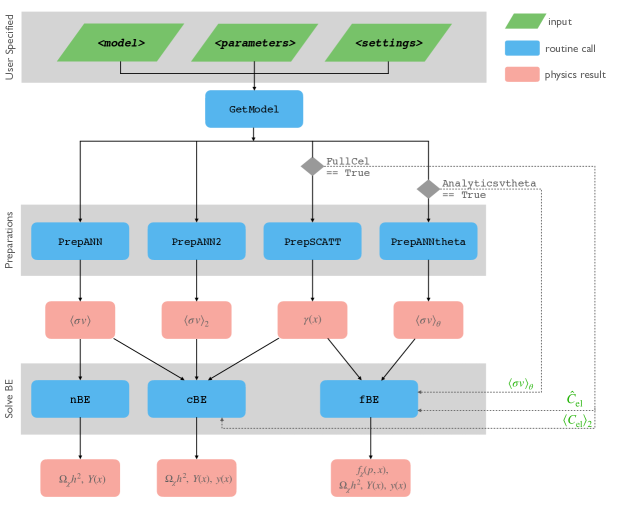
the calculation procedure consists of initializing the DRAKE package, then loading the DM model setup files, performing the required preparatory calculations and finally executing the Boltzmann equation solvers.

A dedicated quick start guide as well as a description of more features and details of DRAKE are provided in Appendix A.

3.2 Numerical implementation

All three Boltzmann equations (nBE, cBE and fBE) are numerically time ($x$) integrated by essentially the same implicit adaptive algorithm. Once the phase-space density is discretized in momentum space as $f_{\chi}(t,p)\rightarrow\{f_{0}(t),...,f_{N}(t)\}$, in particular, all of them can be written as a coupled system of ordinary first order differential equations of the form

$$\frac{\text{d}}{\text{d}x}\mathbf{V}(x)=\mathbf{F}(x,\mathbf{V}),$$ (13)

where $\mathbf{V}(x)=\{V_{0}(x),...,V_{N}(x)\}$ and $\mathbf{F}=\{F_{0}(x,\mathbf{V}),...,F_{N}(x,\mathbf{V})\}$. For concreteness, $\mathbf{V}(x)=Y(x)$ is one-dimensional for nBE, $\mathbf{V}(x)=\{Y(x),y(x)\}$ for cBE as in Eqs. (10) and (2.3), and $\mathbf{V}(x)=\{f_{0}(x),...f_{N}(x)\}$ for the momentum-discretized phase-space density in the fBE approach. We follow standard practice for the numerical integration of these equations, see, e.g., Ref. Nbook .

Concretely, we choose the Adams-Moulton time discretization methods of order one and two, which are also known as the implicit Euler

$$\mathbf{V}_{i}=\mathbf{V}_{i-1}+h\left[\mathbf{F}(x_{i},\mathbf{V}_{i})\right],$$ (14)

and implicit trapezoidal method

$$\mathbf{V}_{i}=\mathbf{V}_{i-1}+\frac{h}{2}\left[\mathbf{F}(x_{i-1},\mathbf{V}_{i-1})+\mathbf{F}(x_{i},\mathbf{V}_{i})\right],$$ (15)

where $\mathbf{V}_{i}\equiv\mathbf{V}(x_{i})$ and $x_{i}=x_{i-1}+h$. The adaptive step size $h$ is controlled through a local relative error of the two methods, $\text{err}_{i}\equiv\underset{j}{\text{Max}}\{\text{Abs}\left[((\mathbf{V}_{i}^{T})_{j}-(\mathbf{V}_{i}^{E})_{j})/(\mathbf{V}_{i}^{T})_{j}\right]\}$ where $\mathbf{V}_{i}^{E}$ and $\mathbf{V}_{i}^{T}$ are the solutions of the implicit Euler Eq. (14) and trapezoidal Eq. (15), respectively. By default, the solution $\mathbf{V}_{i}^{T}$ is accepted if $\text{err}_{i}<10^{-3}$.

For the single number density equation (nBE), the implicit equations (14) and (15) can respectively be solved analytically for $\mathbf{V}_{i}^{T}$ and $\mathbf{V}_{i}^{E}$, allowing for efficient time integration. In this one-dimensional case, thus, the implemented algorithm in our nBE routine is equal to the one used in DarkSUSY.

In the case of cBE and fBE, the solution of Eqs. (14,15) needs to be obtained numerically. A standard root finding algorithm is the Newton iteration method. Defining the iteration depth $n$ and introducing $\mathbf{\Delta}_{i}^{(n+1)}\equiv\mathbf{V}^{(n)}_{i}-\mathbf{V}^{(n+1)}_{i}$, the Newton iteration for the Euler method in Eq. (14) can be written in the form of a linear algebraic problem for $\mathbf{\Delta}_{i}^{(n+1)}$ as

$$\left[\mathbf{1}-h\partial_{\mathbf{V}}\mathbf{F}(x_{i},\mathbf{V}_{i}^{(n)})\right]\mathbf{\Delta}_{i}^{(n+1)}=$$ (16)

$$\mathbf{V}_{i}^{(n)}-\mathbf{V}_{i-1}-h\left[\mathbf{F}(x_{i},\mathbf{V}^{(n)}_{i})\right],$$

and for the trapezoidal method in Eq. (15) as

$$\left[\mathbf{1}-\frac{h}{2}\partial_{\mathbf{V}}\mathbf{F}(x_{i},\mathbf{V}_{i}^{(n)})\right]\mathbf{\Delta}_{i}^{(n+1)}=$$ (17)

$$\mathbf{V}_{i}^{(n)}-\mathbf{V}_{i-1}-\frac{h}{2}\left[\mathbf{F}(x_{i-1},\mathbf{V}_{i-1})+\mathbf{F}(x_{i},\mathbf{V}^{(n)}_{i})\right],$$

where $\partial_{\mathbf{V}}\mathbf{F}$ denotes the ($N+1\times N+1$) Jacobian matrix. The improved value for each iteration can be obtained as $\mathbf{V}^{(n+1)}_{i}=\mathbf{V}^{(n)}_{i}-\mathbf{\Delta}_{i}^{(n+1)}$. At each step in the $x$ integration, we choose the predictor as $\mathbf{V}_{i}^{(0)}=\mathbf{V}_{i-1}$ and iterate each method until the maximum relative error, $\text{errNewton}_{i}^{(n+1)}\equiv\underset{j}{\text{Max}}\{\text{Abs}[(\mathbf{\Delta}_{i}^{(n+1)})_{j}/(\mathbf{V}^{(n+1)}_{i})_{j}]\}$, is one order of magnitude smaller than the upper bound on $\text{err}_{i}$. We also require $\text{errNewton}_{i}^{(n+1)}$ to be smaller or equal to another accuracy control parameter, $\text{errMaxNewton}_{i}=0.4$, at every iteration step; otherwise, the stepsize $h$ is lowered in order to ensure that the Newton iteration converges. Default values for the accuracy control parameters introduced above ($\text{err}_{i}$, $\text{errNewton}_{i}^{(n+1)}$ and $\text{errMaxNewton}_{i}$) can be adopted by changes in the settings file, see Appendix A.5.

For the cBE and fBE routines we have implemented further, automatized performance optimizations. In the two-dimensional cBE case, in particular, we analytically solve in Eqs. (14,15) the corresponding number density equation for $Y_{i}$, Eq. (10), as a function of the DM temperature $y_{i}$, and plug that solution into the DM temperature equation for $y_{i}$, Eq. (2.3). Effectively, this reduces the cBE system to an one-dimensional ordinary differential equation, which is how it is implemented in the cBE routine.

For fBE, the computation of the Jacobian $\partial_{\mathbf{V}}\mathbf{F}$ is implemented in vectorized form. Moreover, all parts in $\mathbf{F}$ that depend only linearly on $\mathbf{V}$, e.g., the scattering operator in Eq. (5), are pre-computed for every time step ($i$) and separated from the ones which need to be updated in every Newton step ($n$).

Furthermore, we implemented two momentum coordinate systems, $A$ and $B$, for different temperature regimes, such that the phase-space density long before and long after kinetic decoupling remains stationary in the respective coordinates (for $Y=const.$). Concretely, the phase-space density is disretized on a uniform grid in $q_{A}\equiv p/\sqrt{m_{\chi}T}$ for $\text{Abs}[1-y^{\text{eq}}/y]<$qATOqB and $q_{B}\equiv(g^{s}_{\mathrm{eff}})^{-1/3}\,p/T$ otherwise. By default, this setting variable is set to qATOqB$=0.1$.

For the momentum derivatives of the phase-space density in Eq. (5) we implemented finite differentiation methods of higher order accuracy using several neighboring points. For central differentiation and fourth order accuracy implemented as a default, the boundary values of the phase-space density used are reflection symmetry at the origin $f_{0}$, introducing the ghost points to obey $f_{-1}(x)=f_{1}(x),f_{-2}(x)=f_{2}(x)$, and vanishing phase-space density at numerical infinity, i.e., $f_{N+1}(x)=f_{N+2}(x)=0$.

In practice we rely on Mathematica’s LinearSolve command for solving Eqs. (16) and (17) in the fBE approach. This part of the code, as well as other time-consuming matrix manipulations like collision term updates, is implemented in a C-compiled environment (if no C compiler is available it is targeted to the Wolfram Virtual Machine), allowing for run-time performances comparable to pure C++ or Fortran code based on the analogue dgesv command from the LAPACK package lapack99 .

3.3 Validity tests

The evolution of the number density $Y(x)$ based on the traditional nBE approach were cross-checked against results obtained with DarkSUSY, for a variety of models ranging from rather generic WIMP realizations to situations where DM annihilates through a narrow resonance. Similarly, the temperature evolution $y(x)$ computed with the kinetic decoupling (only) routines in DarkSUSY was compared to that obtained in DRAKE in the cBE and fBE approaches after switching off annihilation in our code through the settings command KDonly$=$True. For all tested models the results were found to be in agreement at well below the percent level.

We further checked explicitly that the number density evolution in the cBE and fBE approaches correctly coincides with the nBE solution in situations where the effect of kinetic decoupling is irrelevant; e.g. when the DM particles remain in full kinetic equilibrium during the freeze-out process or when the velocity dependence of the annihilation cross-section is insignificant.

The non-trivial interference of chemical and kinetic decoupling, as taken into account in our two beyond-nBE approaches, was meticulously checked against independently implemented codes. In particular, the DRAKE cBE results in the current implementation of the Scalar Singlet model (c.f. footnote 4) were compared to results obtained from FORTRAN routines relying on the sfode sfode solver, finding agreement at the sub-percent level. Furthermore, the fBE results were compared to the phase-space solver originally developed in MatLab based on the ODE15s solver and used in Ref. Binder:2017rgn . For resonance annihilation considered in Section 4.1 for example, very good agreement was found. Note that the cBE and fBE routines in DRAKE do not rely on pre built-in differential equation solvers (see Section 3.2), so all these tests provide an independent validity check.

A final important consistency check of the numerical fBE implementation concerns the question whether the elastic scattering operator in Eq. (5) conserves particle number. While this is manifestly the case in the continuous limit (and hence also in cBE), the discretized version with a finite number and range in momentum can lead to a spurious change of the comoving number density if $\gamma/H\ggg 1$. Therefore some care must be taken in the initial high-temperature regime. One way to reduce these purely numerical artifacts is to increase the number of phase-space density elements, which however affects the run-time of the fBE routine quadratically. We have therefore introduced an upper limit on $\gamma/H$ above which the system is assumed to be in kinetic equilibrium and DRAKE adopts the nBE approach. By default, this upper limit is set to gamcap$=10^{5}$. This value and the number of phase-space elements, qN, can be adopted in the settings file.

For specific problems, optimal accuracy settings for fBE can differ from the default ones. We therefore provide for all examples in Section 4, as well as for the Scalar Singlet Model, suggested settings files. On a standard laptop computer the time to compute the relic density for one parameter point in the fBE approach can range from less than a second to tens of minutes (e.g. in the presence of very narrow resonances).

Furthermore, DRAKE contains example benchmark files with settings adjusted to specific cases, illustrating the usage for more challenging models. For further details concerning those test files see Appendix A.3, as well as Appendix A.5 for accuracy control parameters.

4 Physics scenarios

A velocity-dependent annihilation cross-section is a necessary condition for deviations from the standard computation of the relic abundance, due to the interplay of chemical and kinetic decoupling. In this section we consider three different types of physically well-motivated scenarios where such a velocity-dependence can appear, and where kinetic equilibrium is not necessarily maintained during chemical decoupling. We discuss these scenarios in some detail, both to highlight the non-trivial physics of the freeze-out process in at least parts of the models’ parameter space, and to illustrate how DRAKE can be used to study the freeze-out process beyond the simplifying assumptions usually adopted in the literature.

4.1 Resonant annihilation

As our first example, we consider cases where the annihilation cross-section has a strong velocity dependence induced by an $s$-channel resonance. The effect of early kinetic decoupling for such a setup has been studied in detail in Ref. Binder:2017rgn for the Scalar Singlet model Silveira:1985rk ; McDonald:1993ex ; Burgess:2000yq , where the almost on-shell particle in the $s$-channel is the SM Higgs. For Scalar Singlet masses slightly smaller than half of the Higgs mass it was found that a larger coupling to the Higgs is required to obtain the right relic abundance, which interestingly implies that future measurements of the Higgs-to-invisible decay width can probe more of the parameter region than expected from the standard relic abundance computation, see Refs. Duch:2017nbe ; Hektor:2019ote ; Abe:2020obo for experimental probes and also for other Higgs resonance scenarios with similar effects.

To offer a complementary perspective, we consider here instead a generic vector mediator $A^{\mu}$ inducing an $s$-channel resonance (where the parameter region close to the resonance is particularly interesting from a model-building perspective, see, e.g., Refs. Feng:2017drg ; Bernreuther:2020koj ; Fairbairn:2014aqa ; Pozzo:2018anw ). A minimal version of such a scenario is described by the interaction Lagrangian

$$\mathcal{L}\supset-g_{\chi}\bar{\chi}\gamma^{\mu}\chi A_{\mu}-g_{f}\bar{f}\gamma^{\mu}fA_{\mu}\,,$$ (18)

allowing a Dirac fermion DM particle $\chi$ to resonantly annihilate into heat bath fermions $f$. The model can thus be described by a set of 5 parameters, $(m_{\chi},r,\tilde{\gamma},\delta,\rho)$, where $m_{\chi}$ is the DM mass, $r\equiv m_{f}/m_{\chi}$ defines the mass ratio of heat bath fermions to DM, $\tilde{\gamma}\equiv\Gamma_{A}/m_{A}$ is a dimensionless measure of the total decay width of $A^{\mu}$, $\rho\equiv\sqrt{g_{\chi}g_{f}}$ is the combination of coupling constants relevant for our discussion and $\delta\equiv(2m_{\chi}/m_{A})^{2}-1$ measures the deviation from the exact resonance position (at $\delta=0$).

With these definitions, the annihilation cross-section for this process, $\chi\bar{\chi}\rightarrow A^{\star}\rightarrow f\bar{f}$, can be written as

$$\sigma v_{\rm lab}=\frac{\rho^{4}}{384\pi m_{\chi}^{2}}\frac{(1-r^{2}/\tilde{s})^{1/2}(1+\delta)^{2}}{2\tilde{s}-1}\alpha(\tilde{s})D(\tilde{s})\,,$$ (19)

with $\alpha(\tilde{s})=4(2\tilde{s}+1)(2\tilde{s}+r^{2})$ and $\tilde{s}\equiv s/(4m_{\chi}^{2})$, where $\sqrt{s}$ is the center-of-mass energy, and the resonance is encoded in the Breit-Wigner propagator

$$D(\tilde{s})\equiv\frac{1}{\left[\tilde{s}(1+\delta)-1\right]^{2}+\tilde{\gamma}^{2}}.$$ (20)

The scattering amplitude for $\chi f\leftrightarrow\chi f$ in the non-relativistic limit, $\tilde{s}\to(1+r^{2}+2\omega/m_{\chi})/4$, on the other hand, is given by

$$|\mathcal{M}|^{2}_{\chi f\leftrightarrow\chi f}=\frac{16(\delta+1)^{2}\rho^{4}}{\left(t(1+\delta)-4m_{\chi}^{2}\right)^{2}}\beta(\omega,t)\,,$$ (21)

where

$$\beta(\omega,t)=8m_{\chi}^{2}\omega^{2}+4m_{\chi}^{2}\left(\frac{\omega}{m_{\chi}}+\frac{1}{2}+\frac{r^{2}}{2}\right)t+t^{2}\,.$$ (22)

Following our standard convention, Eq. (21) is summed over both in- and out-going spin states, as well as particle and anti-particle states of the scattering partners $f$.

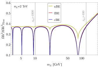
We will concentrate here on the parameter region $|\delta|<1$ where the annihilation cross-section is resonantly enhanced. This implies that $\rho$ must be suppressed in order to obtain the correct relic abundance, leading to a corresponding suppression of the scattering amplitude. On top of that, the momentum transfer rate $\gamma(x)$ can be further Boltzmann suppressed for sufficiently massive scattering partners. In combination, these effects can lead to very early kinetic decoupling, interfering with the chemical decoupling process. In Fig. 2

Figure 2: The relic abundance, for a model with resonant annihilation, in the cBE (blue) and fBE (red) treatments, relative to that of the standard approach (nBE), as a function of the distance $\delta$ to the resonance. The different line style indicates different mass ratios $r=m_{f}/m_{\chi}$. In this example, $m_{\chi}=1$ TeV, $\tilde{\gamma}=10^{-5}$ and coupling values are fixed by the requirement $2(\Omega_{\chi}h^{2})_{\rm nBE}=\Omega_{\rm DM}h^{2}$. The inset plots show zoom-ins of the resonant region around $\delta=0$.

we quantify the impact on the relic abundance in such a situation, choosing for definiteness a fixed DM mass of $m_{\chi}=1$ TeV and a resonance width of $\tilde{\gamma}=10^{-5}$. Here, we fix the coupling $\rho$ in every parameter point such that the conventional approach (nBE) matches the value of the observed DM abundance, i.e., $2(\Omega_{\chi}h^{2})_{\rm nBE}=\Omega_{\rm DM}h^{2}=0.120$. Clearly, the cBE and fBE approaches demonstrate significant corrections to the standard treatment. As expected, the larger the mass ratio $r$ (from dotted to dashed to solid lines), the earlier DM decouples and the stronger the effect becomes. Even for very light heat bath particles, however, the correction to the standard result remains sizeable (for $r<0.1$, the resulting curves do not significantly differ from the $r=0.1$ case displayed in Fig. 2). The characteristic two-bump feature and the narrow dip around the exact resonance position at $\delta=0$ are a consequence of different DM cooling and heating effects during the chemical evolution that affect the DM phase-space distribution $f_{\chi}(x,p)$. The phenomenology of coupled chemical and kinetic evolutions here is very similar to the Scalar Singlet DM example, and for a detailed discussion of the origin of these features we refer to to Appendix A in Ref. Binder:2017rgn .

In Fig. 3,

Figure 3: Contour lines of constant $(\Omega_{\chi}h^{2})_{\rm fBE}/(\Omega_{\chi}h^{2})_{\rm nBE}$ in the $\delta-\tilde{\gamma}$ plane for a model with $m_{\chi}=1$ GeV and $r=0.3$. As in Fig. 2, couplings are fixed such that $2(\Omega_{\chi}h^{2})_{\rm nBE}=\Omega_{\rm DM}h^{2}$, and $\delta=(2m_{\chi}/m_{A})^{2}-1$. Red (blue) colors highlight regions where the early kinetic decoupling effect overall increases (decreases) the predicted relic abundance compared to the standard treatment. Dotted black lines show, for comparison, the widths of the SM $Z^{0}$ and Higgs bosons. The gray shaded areas on the edges of the plot indicate parameter regions where the $\rho$ value satisfying the relic density condition cannot be achieved without violating perturbativity or by extending the model (see text for more details).

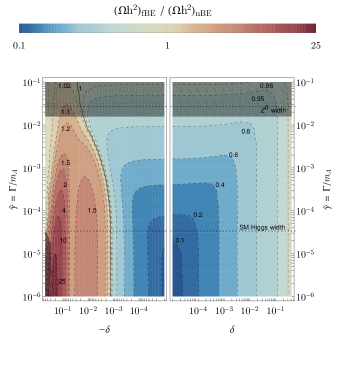
we complement this discussion by showing the impact on the relic abundance when instead varying the resonance width $\tilde{\gamma}$ and keeping the mass ratio $r$ fixed. This leads to a structure that is straightforward to relate to what is visible in the previous figure; for example, the two distinctive peak regions in the bottom left corner correspond to the two peaks in Fig. 2 (note however that here we consider a much lighter DM particle, $m_{\chi}=1$ GeV, than in Fig. 2). For most of the parameter space, a smaller width generally leads to a larger effect, i.e. larger deviations from the standard computation. It is interesting to note that even for widths as large as that of the SM $Z$-boson the refined prediction of the DM abundance can deviate at a level well exceeding the typically quoted observational uncertainty of $\sim 1$% in $\Omega_{\rm DM}h^{2}$ — and hence at a level that would, e.g., affect global fits in a noticeable way.

It is worth noting that for the simple model considered here, not every pair of values $(\delta,\tilde{\gamma})$ shown in Figs. 2 and 3 may be a consistent choice. Indeed, the minimal contribution to the width, from the interaction Lagrangian in Eq. (18), is given by

$$\tilde{\gamma}=\sum_{i=\chi,f}\frac{g_{i}^{2}}{12\pi}\left(1+\frac{2m_{i}^{2}}{m_{A}^{2}}\right)\sqrt{1-\frac{4m_{i}^{2}}{m_{A}^{2}}}\,.$$ (23)

In Fig. 3 we indicate (with gray shaded regions) the values of $(\delta,\tilde{\gamma})$ that cannot be satisfied by Eq. (23) when $\rho=\sqrt{g_{\chi}g_{f}}$ is fixed by the relic density condition (either because Eq. (23) would imply a larger value of $\tilde{\gamma}$ than required, or because at least one of the couplings would no longer satisfy $g_{\chi},g_{f}<\sqrt{4\pi}$, thus indicating a breakdown of perturbativity).

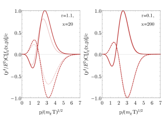
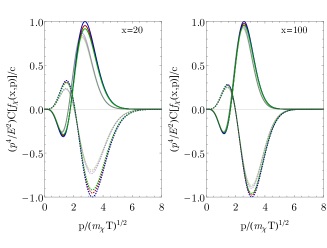
Let us finally remark that the more narrow the resonance, the more momentum-selective is the annihilation process. This can lead to shapes of the distribution function that strongly differ from thermal ones. As a concrete example, we demonstrate in Fig. 4

Figure 4: Time evolution of the phase-space density $f_{\chi}(x,q)$, computed by the fBE approach. The color scale shows the DM abundance $Y(x)$, in units of its final value, which reflects the overall normalization of $f_{\chi}$. This example is for a case of DM annihilation through a narrow resonance and an early kinetic decoupling (with model parameters stated in the legend). The coupling strength is set to $\rho=1.13\times 10^{-2}$ in order to satisfy $2(\Omega_{\chi}h^{2})_{\rm fBE}=\Omega_{\rm DM}h^{2}$. The initial equilibrium phase-space distribution is strongly distorted during chemical and kinetic decoupling, and finally remains in a highly non-thermal shape.

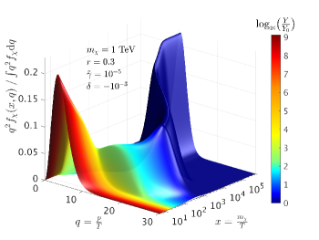
that the fBE approach implemented in DRAKE can accurately resolve such non-trivial phase-space evolutions even for extremely narrow resonances (in this example a factor of a few below the Higgs width).

4.2 Sommerfeld-enhanced annihilation

As our second example, we consider a case where DM annihilation is Sommerfeld-enhanced due to the presence of a light mediator. Physically, such a light mediator induces a long-range Yukawa potential between the DM particles that modifies their wave function, leading to a non-perturbative enhancement of the tree-level annihilation rate Hisano:2002fk ; Hisano:2003ec ; Hisano:2004ds ; Hisano:2006nn ; Cirelli:2007xd ; Mitridate:2017izz . Because the Sommerfeld effect is strongly velocity-dependent, it provides a prime example of interest to study the interplay of chemical and kinetic decoupling Dent:2009bv ; Zavala:2009mi ; Feng:2010zp ; vandenAarssen:2012ag . In fact, this is the context in which coupled Boltzmann equations akin to our Eqs. (10,2.3) have first been proposed vandenAarssen:2012ag .

For simplicity, we consider the same model Lagrangian as in the previous section, Eq. (18), but now in a very different parameter region. Concretely, we will assume $m_{A}\lesssim\alpha_{\chi}m_{\chi}$, with $\alpha_{\chi}\equiv g_{\chi}^{2}/(4\pi)$, such that the vector mediator induces a long-range force. Furthermore, we take the heat bath particles $f$ to be (approximately) massless and only milli-charged under the broken $U(1)^{\prime}$, in the sense that $g_{f}\ll g_{\chi}$. Consequently, $\chi\bar{\chi}\to AA$ is the leading annihilation process. The corresponding tree-level cross-section, expanded up to leading order in $v\ll 1$ and $m_{A}/m_{\chi}\ll 1$, is given by $(\sigma v_{\rm lab})_{0}\simeq\pi\alpha^{2}_{\chi}/m_{\chi}^{2}$. We explicitly checked that this approximation holds for the range of parameters that we will consider here. The full $s$-wave annihilation cross-section including the Sommerfeld effect is then obtained as

$$\sigma v_{\rm lab}=S(v_{\rm lab})\times(\sigma v_{\rm lab})_{0}\,,$$ (24)

where we use the analytical expressions for the Sommerfeld enhancement factor $S(v_{\rm lab})$ that were obtained, e.g., in Ref. Cassel:2009wt ; Slatyer:2009vg after approximating the Yukawa potential by a Hulthén potential:

$$S(v_{\rm lab})=\frac{\frac{\pi}{\epsilon_{v}}\sinh\!\Big{[}\frac{12\epsilon_{v}}{\pi\epsilon_{A}}\Big{]}}{\cosh\!\Big{[}\frac{12\epsilon_{v}}{\pi\epsilon_{A}}\Big{]}-\cos\!\Big{[}2\pi\sqrt{\frac{6}{\pi^{2}\epsilon_{A}}\!-\!\left(\frac{6\epsilon_{v}}{\pi^{2}\epsilon_{A}}\right)^{2}}\Big{]}},$$ (25)

where $\epsilon_{v}\equiv v_{\text{lab}}/(2\alpha_{\chi})$ and $\epsilon_{A}\equiv m_{A}/(\alpha_{\chi}m_{\chi})$.

We concentrate on the parameter region where $g_{f}$ is (just) large enough for the mediator to be in equilibrium during freeze-out, established by the decay and inverse decay processes $A\leftrightarrow f\bar{f}$. Requiring the decay rate to satisfy $\Gamma_{A\rightarrow f\bar{f}}/H\gtrsim 1$ for $T\lesssim m_{\chi}$, one finds that this is realized for $g_{f}\gtrsim 3\times 10^{-6}(0.1/r_{A})(m_{\chi}/\text{TeV})^{1/2}$, where $r_{A}\equiv m_{A}/m_{\chi}$. For simplicity we will exclusively focus on coupling values that are not significantly larger than this lower bound, thus implementing the earliest possibility when DM can kinetically decouple in this model. In this case, Coulomb-like scattering processes $f\chi\leftrightarrow f\chi$ can be neglected – as we checked explicitly – and DM is kept in kinetic equilibrium by the Compton-like scattering with the vector particle, $\chi A\leftrightarrow\chi A$. The corresponding scattering amplitude is for non-relativistic DM given by

$$|\mathcal{M}|^{2}_{\chi A\leftrightarrow\chi A}=\frac{8g_{\chi}^{4}\beta(\omega,t)}{(2m_{\chi}\omega+m_{A}^{2})^{2}(2m_{\chi}\omega-m_{A}^{2}+t)^{2}}\,,$$ (26)

where, to leading order in the DM mass,

$$\beta(\omega,t) \simeq 4m_{\chi}^{4}(4m_{A}^{4}-4m_{A}^{2}t+8\omega^{4}+4\omega^{2}t+t^{2}).$$ (27)

In this parameter region, the phenomenology of the model thus only depends on the coupling $g_{\chi}$ (unlike in the previous section, where the relevant coupling combination was $\rho=\sqrt{g_{\chi}g_{f}}$). For relevant coupling values and the scattering amplitude as in Eq. (26), kinetic decoupling occurs once the vector boson $A$ enters the non-relativistic regime, causing a Boltzmann suppression of the momentum transfer rate $\gamma(x)$.

In Fig. 5

Figure 5: Relic abundance for the Sommerfeld-enhanced annihilation example, for a fixed DM mass of $m_{\chi}=2$ TeV and as a function of the mediator mass $m_{A}$. The coupling is fixed to $\alpha_{\chi}=0.07$ from the requirement $2(\Omega_{\chi}h^{2})_{\text{Tree}}=\Omega_{\text{DM}}h^{2}$, based on the (velocity-independent) tree-level annihilation cross-section $(\sigma v_{\rm lab})_{0}$ without Sommerfeld enhancement. The predictions from the traditional nBE computation clearly demonstrate the impact of the Sommerfeld effect on the annihilation rate, while the improved calculations based on cBE and fBE quantify the additional impact of kinetic decoupling on the relic abundance.

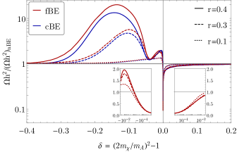
we show the resulting relic density in this setup, for a range of mediator masses $m_{A}$ and fixed DM mass ($m_{\chi}=2$ TeV) and coupling ($\alpha_{\chi}=0.07$). As is clearly visible in this figure, the Sommerfeld effect alone affects the relic density by a factor of 2–3 compared to the tree-level expectation. For selected values of mediator masses, the difference between the standard approach and both our beyond-nBE approaches can be even larger. For these parameter combinations, bound states with zero binding energy can form; parametrically, these exist precisely at threshold for $m_{A}/(\alpha_{\chi}m_{\chi})=6/(n^{2}\pi^{2})$ in the case of the Hulthén potential (with $n\in\mathbb{Z}^{+}$). Close to these parametric resonances the Sommerfeld effect scales as $S(v_{\rm lab})\propto 1/v_{\rm lab}^{2}$ for $v_{\rm lab}\lesssim m_{A}/m_{\chi}$, leading to a second period of annihilation after kinetic decoupling Dent:2009bv ; Zavala:2009mi ; Feng:2010zp ; vandenAarssen:2012ag . We illustrate this in Fig. 6

Figure 6: Evolution of DM abundance $Y(x)$ (left) and velocity dispersion $y(x)$ (right) for the Sommerfeld model, with $\alpha_{\chi}$ and $m_{\chi}$ as in Fig. 5. Line colors correspond to nBE (green), cBE (blue) and fBE (red). Line styles refer, as indicated, to different values of $m_{A}$, chosen such that $n^{2}=6\alpha_{\chi}m_{\chi}/(\pi^{2}m_{A})$ is close to integer (parametric resonance condition). The second annihilation era characteristic for these models is clearly visible as a drop of $Y$ in the left panel; the corresponding increase in the DM temperature visible in the right panel is caused by a self-heating due to efficient annihilation out of thermal equilibrium.

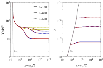
by plotting the evolution of the DM abundance $Y(x)$ for three selected mediator masses close to such a parametric resonance (left panel). Due to the inverse velocity dependence of $S(v_{\rm lab})$, furthermore, DM particles prefer to annihilate at smaller momenta, leading to a self-heating after kinetic decoupling and hence an increase in $y(x)$ (right panel) – see also the discussion in Ref. vandenAarssen:2012ag .

Inspecting Fig. 5, we find significant deviations from the standard computation also for parameter regions further away from the exact resonance condition. Here, the Sommerfeld effect scales only as $S(v_{\rm lab})\propto 1/v_{\rm lab}$, which correspondingly leads to a significantly weaker re-annihilation effect. Let us point out that even for situations with a relatively early kinetic decoupling as studied in this section (though still much later than what we studied in Section 4.1), the difference between cBE and fBE is as expected rather small, independently of the vicinity to a parametric resonance. This holds both for the evolution of the number density and that of the DM temperature, as also demonstrated earlier in Ref. Binder:2017lkj .

In general, the effect on the DM abundance due to kinetic decoupling is of course larger for earlier kinetic decoupling (assuming all other parameters to be fixed). However, we remark that even for later kinetic decoupling than in the minimal case discussed here – e.g. in the case where Coulomb-like scattering dominates, for much larger coupling values $g_{f}$ – the correct prediction of $\Omega_{\chi}h^{2}$ can be sensitive to the interplay of kinetic and chemical freeze-out processes, making it necessary to go beyond the traditional nBE approach.

4.3 Sub-threshold annihilation

As our final example we consider a situation where the annihilation process that sets the relic density is kinematically not accessible in the limit of vanishing velocities, sometimes dubbed ‘forbidden’ DM DAgnolo:2015ujb .

For concreteness, we adopt a simple scenario with an interaction Lagrangian given by

$$\mathcal{L}\supset-\frac{\lambda}{4}\phi_{1}^{2}\phi_{2}^{2}+y_{f}\phi_{2}\bar{f}f\,,$$ (28)

where the scalar $\phi_{1}$ takes the role of the DM particle. It directly interacts only with the scalar $\phi_{2}$, which we assume to be close in mass with $\phi_{1}$, i.e., $r\equiv m_{2}/m_{1}\sim 1$, and to be in thermal contact with the heat bath fermions $f$. To lowest order, the total DM annihilation cross-section is determined by the process $\phi_{1}\phi_{1}\to\phi_{2}\phi_{2}$, and given by

$$(\sigma v_{\rm lab})^{2\to 2}=\frac{\lambda^{2}}{32\pi}\frac{\sqrt{1-4m_{2}^{2}/s}}{s-2m_{1}^{2}}\,.$$ (29)

For $r>1$, this process is only open to particles in the high-energy tail of the DM distribution, leading to an exponential suppression of $\langle\sigma v\rangle$ and a corresponding increase of $\Omega_{\chi}h^{2}$.

Similar to the Sommerfeld enhancement example discussed in the previous section, we restrict our discussion for simplicity to couplings $y_{f}$ (just) large enough to bring $\phi_{2}$ into equilibrium before the onset of the freeze-out process, through (inverse) decays $\phi_{2}\leftrightarrow\bar{f}f$. Demanding for concreteness $\Gamma_{\phi_{2}\leftrightarrow\bar{f}f}/H\gtrsim 1$ for $T\lesssim m_{1}$, this requires $y_{f}\gtrsim 10^{-7}\,r^{-\frac{1}{2}}\left(m_{1}/{\rm TeV}\right)^{\frac{1}{2}}$. At the same time we require for consistency that $y_{f}$ is small enough such that i) close to the threshold at $r\sim 1$, 3-body processes of the form $\phi_{1}\phi_{1}\to\phi_{2}\phi_{2}^{*}\to\phi_{2}f\bar{f}$ can be neglected and that ii) the loop-induced scattering with $f$ is subdominant compared to the tree-level scattering with the Boltzmann-suppressed $\phi_{2}$ particles, via $\phi_{1}\phi_{2}\leftrightarrow\phi_{1}\phi_{2}$. In this parameter region, the momentum transfer rate, Eq. (5), is then given by

$$\gamma(x)\approx m_{1}\frac{\lambda^{2}}{6\pi^{3}}\frac{r^{2}}{(1+r)^{4}}x^{-2}e^{-rx}\,.$$ (31)

We note that this expression explicitly features the already mentioned exponential suppression due to scattering with non-relativistic $\phi_{2}$ particles. Hence, we expect kinetic decoupling to happen very early in this model, around the time of chemical decoupling.

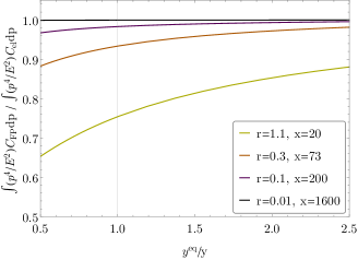
As already stressed in Section 2.2, however, the approximate scattering collision term in Eq. (5), including the momentum transfer rate, relies on the assumption of small momentum transfer compared to the average DM momentum – which is typically not satisfied for scattering partners that are close in mass to the DM particle. For the simple case of a constant scattering amplitude, consistent with our interaction Lagrangian in Eq. (28), we demonstrate in Appendix B that it is possible to instead implement the scattering collision term $C_{\text{el}}$ without this assumption. Concretely, we perform analytically all integrals for $W$ in Eq. (8) , c.f. Eq. (33), and use this expression to compute $C_{\text{el}}$ in Eq. (7). This allows us to contrast our results to those based on the approximate scattering term $C_{\text{FP}}$ (relying on small momentum transfer).

In Fig. 7

Figure 7: Relic abundance for the sub-threshold annihilation example, for a fixed DM mass of $m_{1}=100$ GeV and in function of the final state mass ratio $r=m_{2}/m_{1}$. The value of the $\phi_{1}-\phi_{2}$ coupling, $\lambda$, is determined by the requirement $(\Omega_{\chi}h^{2})_{\text{nBE}}=\Omega_{\text{DM}}h^{2}$; in the ‘forbidden’ region, for $r>1$, $\lambda$ is thus exponentially sensitive to $r$. Solid red (blue) lines correspond to results from the fBE (cBE) treatment based on the full scattering term of this example, while the corresponding results based on the small-momentum transfer approximation in Eq. (5) are plotted with lighter shading.

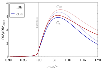
we plot the relic density that results from the fBE and cBE approaches, with different implementations of the scattering terms, relative to that from the nBE approach. Here, for each value of $r$, the coupling $\lambda$ is fixed by the requirement that the standard nBE prediction matches the observed abundance. As is clearly visible, early kinetic decoupling can have a significant impact on the relic abundance also for this threshold example, at least for $r\gtrsim 1$. While it is remarkable that both scattering term prescriptions show qualitatively the same result, however, in this model DM turns out to be kept slightly more efficiently in kinetic equilibrium with the more correct $C_{\text{el}}$ approach; see also Fig. 10 in Appendix B. This explains why the $C_{\text{el}}$ prescription leads to a relic density slightly closer to that of the standard nBE approach than what we find with the Fokker-Planck approximation.

In Fig. 8,

Figure 8: Evolution of DM abundance $Y(x)$ (left) and velocity dispersion $y(x)$ (right) for the sub-threshold model with three selected values of $r$. DM mass and couplings are fixed as in Fig. 7, and line styles chosen in accordance with that figure. For these threshold examples, DM needs high momenta for annihilation to be kinematically allowed, which results in a phase of cooling around and after kinetic decoupling, and hence a drop in $y(x)$.

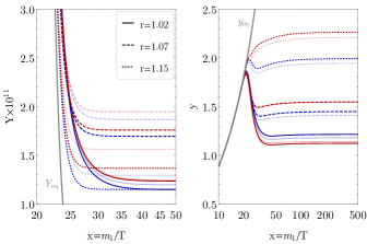
we show the abundance and temperature evolution for selected values of $r>1$. Qualitatively, DM needs higher momenta to overcome the annihilation threshold, leading to a self-cooling phase as soon as it is no longer (fully) kinetically coupled to the particles $\phi_{2}$ that remain in equilibrium with the heat bath. Due to this cooling, annihilation becomes less efficient earlier, resulting in a higher DM abundance than in the standard computation.

Let us close this section by briefly mentioning again that the kinematically suppressed annihilation cross-section implies that the coupling $\lambda$ must grow exponentially with $r$ in order to maintain the correct DM abundance. For example, in the nBE approach with $m_{1}=100$ GeV very large couplings $\lambda\gtrsim 4\pi$ are reached at $r\gtrsim 1.2$; for the cBE and fBE approaches this happens at even smaller values of $r$, closer to the peak visible in Fig. 7.

5 Summary

Thermal freeze-out is widely considered one of the most intriguing mechanisms for the production of DM. The underlying assumption of by far most relic density calculations in the literature is that kinetic equilibrium is maintained during the freeze-out. Here we have presented a new public tool, DRAKE, to explicitly gauge the impact of this assumption in cases where it might not be valid. To do so, the code offers various alternative schemes to calculate the relic density that take into account the intriguing effects of kinetic decoupling during the chemical freeze-out process, including a full calculation at the phase-space level.

In fact, it has repeatedly been pointed out that chemical and kinetic decoupling can be intertwined in a way that significantly affects the result of relic density calculations vandenAarssen:2012ag ; Duch:2017nbe ; Kamada:2017gfc ; Berlin:2018tvf ; Kamada:2018hte ; Abe:2020obo ; Binder:2017rgn ; Brummer:2019inq ; Ala-Mattinen:2019mpa ; Kuflik:2015isi ; Kuflik:2017iqs ; Fitzpatrick:2020vba ; Biswas:2020ubd ; Croon:2020ntf . To provide context, we have therefore devoted a large part of this article (Section 4) to a comprehensive and updated study of three physically well-motivated scenarios of annihilating DM where this is the case, illustrating the need to move beyond the standard treatment and demonstrating that this is possible without compromising on accuracy. This is clearly important for global fits that include parameter regions in their scans where the interplay between kinetic and chemical equilibrium cannot be neglected, but can turn out to be relevant also in various model-building considerations.

Let us finally stress that, while the main focus of DRAKE is the relic density, its output is by no means restricted to a single number. Rather, it allows to compute the full time evolution of the DM phase-space density, or its lowest moments, which may be connected to further late-time observables. For example, a non-standard velocity distribution would affect how free streaming impacts the matter power spectrum of density perturbations Boyanovsky:2010pw ; Hager:2020une , which is one of the main motivations for why linear perturbation solvers like CLASS Lesgourgues:2011rh explicitly support externally tabulated (non-standard) phase-space densities. An exploration of such effects in the context of kinetic decoupling interfering with chemical decoupling would be warranted, but beyond the scope of this work.

Appendices

​​ A Getting started

DRAKE can be downloaded as a zipball from drake.hepforge.org. The only prerequisite for using it is to have Mathematica or the free Wolfram Engine installed.

A.1 Quick start

Unpack the zipball and open the Mathematica notebook main.nb located in the main directory. This example program demonstrates the loading of the DRAKE package, code usage, printing routine output in form of plots, and saving the results. In the following, we expand on the description of all the consecutive steps in this example program.

To load the package, start a fresh kernel and execute

⬇

SetDirectory["<path>"];

Needs["DRAKE`"]

where <path> is the path to the main directory. From this point on, all new symbols can be listed with

⬇

Names["DRAKE`*"]

and documentation of the main functions and variables are provided with the usual syntax, e.g., calling ?cBE returns information about the cBE routine.

All input quantities can be loaded with the command

⬇

GetModel["<model>", "<parameters>", "<settings>"];

The three arguments are names of files (without their extension .wl), located in the sub-directory ./models/<model>/. DRAKE comes with a set of pre-implemented models, where <model> $\in\{$ScalarSingletDM, WIMP, VRES, SE, TH$\}$. The first element in this set is the Scalar Singlet DM model, the second is a WIMP-like test model, while the last three are the scenarios presented in Section 4. For any of these models, choose one of the parameter files <parameters> $\in\{$bm1, bm2, bm3$\}$, implementing different benchmark values of model parameters. Correspondingly, the files <settings>$\in\{$settings_bm1, settings_bm2, settings_bm3$\}$ contain suggested values of accuracy control parameters and Boolean variables for run options.

After these initialization steps, the main DRAKE routines are ready to perform $\Omega_{\chi}h^{2}$ computations. For results obtained with the nBE approach, e.g., this amounts to calling

⬇

PrepANN;

nBE

for any of the pre-implemented models. In the default usage with the Fokker-Planck approximation for $C_{\text{el}}$, on the other hand, the cBE approach consists of the calls

⬇

PrepANN;

PrepANN2;

PrepSCATT;

cBE

and the default fBE approach consists of the calls

⬇

PrepANNtheta;

PrepSCATT;

fBE

When working with all approaches simultaneously, it is sufficient to call each preparatory routine once. Optional procedures, where e.g. PrepANNtheta and PrepSCATT are omitted, are explained in Section A.5.

The output of the preparatory routines and Boltzmann solvers is summarized in Table 3.

Call	Output	Output names
PrepANN	$\langle\sigma v\rangle$	tsv,svx[x]
PrepANN2	$\langle\sigma v\rangle_{2}$	tsv2,sv2x[x]
PrepANNtheta	$\langle\sigma v\rangle_{\theta}$	tsvtheta,
		isvtheta
PrepSCATT	$\gamma(x)$	tgamma,gam[x]
nBE	$(\Omega_{\chi}h^{2})_{\text{nBE}}$	Oh2nBE
	$Y_{\rm nBE}(x)$	tYnBE={x,$Y_{\rm nBE}$}
cBE	$(\Omega_{\chi}h^{2})_{\text{cBE}}$	Oh2cBE
	$Y_{\rm cBE}(x)$	tYcBE={x,$Y_{\rm cBE}$}
	$y_{\rm cBE}(x)$	tycBE={x,$y_{\rm cBE}$}
fBE	$(\Omega_{\chi}h^{2})_{\text{fBE}}$	Oh2fBE
	$Y_{\rm fBE}(x)$	tYfBE={x,$Y_{\rm fBE}$}
	$y_{\rm fBE}(x)$	tyfBE={x,$y_{\rm fBE}$}
	$q^{2}f_{\chi}(x,q)$	tfDM={x,{$q^{2}f_{\chi}$}}

Table 3: Output summary of DRAKE routines. The last column lists the main output variables, tables, and functions stored in the kernel session memory after calling the routine. Cross-section outputs are in units of $\text{GeV}^{-2}$ and $\gamma$ in GeV. All output names starting with ‘t’ are tables and names with an [x] dependence are interpolating functions based on these tables. The tables of the Boltzmann solvers contain all computed $Y$ and $y$ values from initial to final $x$ except tfDM, which contains for memory reason only snapshots of the unity-normalized phase-space density at the initial, intermediate (when switching from momentum coordinates $q_{A}$ to $q_{B}$, see Section 3.2) and final $x$ value. The preparatory routines are stored in the file rates.wl and the Boltzmann solvers in nBE.wl, cBE.wl, and fBE.wl files in the DRAKE source directory.

All listed output variables are stored in the kernel session memory and can be directly accessed and saved to a file <outfile> with, e.g., DRAKE’s command save["<outfile>"].

Values of any model or setting parameters can be changed actively during a notebook session. This makes scans over, e.g., the DM mass simple to perform. Alternatively, one can create different <parameters> and <settings> files and repeatedly use GetModel.

A.2 Template script

The release also contains a template script main.wls, which serves as a streamlined and customizable way to use DRAKE directly from a terminal. For any of the five pre-implemented models (see Section A.1 for file names), in particular, the template script can be executed as

⬇

> wolframscript main.wls <model> <parameters> <settings>

This loads DRAKE, executes GetModel and runs the nBE, cBE, and fBE approaches with a minimum amount of routine calls and according to the user’s option settings (discussed in Section A.5). Figure 1, in Section 3, graphically illustrates its workflow. Results stored in the session’s memory are then saved to a file, with name and path specified in the <settings> file. Important results are also directly displayed in text format, along with the computation time. The template script can also be called in a notebook environment with a convenient wrapper RunMain, as demonstrated in main.nb.

A.3 Tests

The release contains a test notebook, test.nb, located in the "./test" sub-directory. It can be used for checking the DRAKE installation against pre-computed results. While for the simplest pre-implemented model (WIMP) the calculation takes seconds, it can take up to several minutes for the most complicated benchmark scenario (VRES, close to a narrow resonance). The computational time of the Boltzmann solvers is typically less than it takes for the corresponding preparatory routine calls.

For Wolfram Engine users, move to the "./test" directory and run the test script by, e.g.,

⬇

> wolframscript test.wls WIMP bm_WIMP settings_WIMP

which displays the test results for the WIMP model.

A.4 Adding a new model

For adding a new model, choose a model name and run

⬇

AddModel["<modelname>"];

A sub-directory <modelname> is then created in "<path>/models", including new model, parameter and setting files. For default usage, fill out the template functions sv[s_]:= ... ; $[\sigma v_{\text{lab}}(s)]$ and gam[x_]:= ... ; $[\gamma(x)]$ in the model file, specify the DM mass mDM= ... ; ($m_{\chi}$) and internal degrees of freedom gDM= ... ; ($g_{\chi}$) in the parameter file, and save the changes. After these four necessary specifications, the new model can already be used as described in Section A.1, or with the template script as in Section A.2. Note that the setting file can require some accuracy control parameter adaption for optimal usage, see Section A.5 for rather detailed checks. For optional usage (e.g., beyond Fokker-Planck approximation), uncomment the template routines in the model file, specify model dependent parts at the highlighted places, and change Boolean variables in the settings file according to Section A.5.

To create the new model from a terminal execute

⬇

> wolframscript AddModel.wls <modelname>

A.5 Settings

Code settings are stored in <settings> files for all pre-implemented models. These consist of accuracy control parameters and Boolean variables for optional code usage. A possible way of directly checking the effect of these parameters is to plot the output variables of the relevant routines, as listed in Table 3. All parameters introduced in this section are also briefly described in the <settings> files.

Options

The options for preparatory and Boltzmann solver routines are determined by a set of global Boolean variables. In particular, the Boolean variable RelThermalAv determines how $\sigma v_{\text{lab}}$ is averaged in the PrepANN and PrepANN2 routines. If set to true, $\sigma v_{\text{lab}}$ must be provided as a function of the Mandelstam $s$ variable and averages are computed fully relativistically as in Ref. Gondolo:1990dk ; Binder:2017rgn . Setting RelThermalAv to false, $\sigma v_{\text{lab}}$ must be provided as a function of $v_{\text{lab}}$, and the calls PrepANN and PrepANN2 compute averages in the highly non-relativistic limit, as in Ref. vandenAarssen:2012ag . The Sommerfeld enhanced annihilation scenario, as described in Section 4.2 and implemented in SE.wl, is one example where $\sigma v_{\text{lab}}$ is a sufficiently smooth function for accurate non-relativistic thermal averages. Especially for PrepANN2 this is of great advantage since the amount of numerical integrals to be performed is reduced to one vandenAarssen:2012ag .

The Boltzmann solvers cBE and fBE can take optional routines as input. These are summarized in Table 4.

Routine (substitutes)	Implements	Returns
GetAnnMatrixAnalytic	$\langle\sigma v\rangle_{\theta}$	$\langle\sigma v\rangle_{\theta}$
(PrepANNtheta)		(as matrix)
GetScatMatrix	$\langle W\rangle_{\tilde{\Omega}}$	$\hat{\mathbf{C}}_{\text{el}}$
(PrepSCATT for fBE)		[see Eq. (36)]
GetSecondMomentScat	$\langle W\rangle_{\tilde{\Omega}}$	$\langle C_{\text{el}}\rangle_{2}$,
(PrepSCATT for cBE)		$\langle C_{\text{el}}\rangle_{2}^{\prime}$

Table 4: Optional input routines that can be provided in a <model> file. The routine output shown here is symbolic and we refer to the model file TH.wl for a more detailed description.

The first routine allows for directly implementing $\langle\sigma v\rangle_{\theta}$ – especially useful if the angular average can be performed analytically. By setting the Boolean variable Analyticsvtheta in <settings> to true, fBE then adopts this first optional routine, making the call to PrepANNtheta redundant. The other two routines implement $\langle W\rangle_{\tilde{\Omega}}$ and allow for $C_{\text{el}}$ usage beyond the Fokker-Planck approximation. This is activated in cBE and fBE, if FullCel is set to true in <settings>. PrepSCATT calls are then redundant. For a concrete example implementing all these optional routines, see TH.wl (threshold annihilation, as in Section 4.3).

Lastly, if the Boolean variable KDonly is true, annihilation is switched off, and one can investigate kinetic decoupling only (see, e.g., Ref. Bringmann:2009vf ) with the cBE and fBE routines. All preparing routine calls for annihilation are then redundant. For the fBE routine, this also allows to check accuracy settings, see Section 3.3.

Accuracy control parameters

The accuracy of preparatory and Boltzmann solver routines is controlled by a set of global parameters. In particular, the accuracy parameters introduced in Section 3.2 translate to DRAKE internal names as follows. The local maximum error, $\text{err}_{i}$, is stored in nBEerr, cBEerr and fBEerr. Code-internal names for $\text{errNewton}_{i}^{(n+1)}$ (controlling the Newton iterations) are cBEerrNewton and fBEerrNewton. The maximum relative change for any Newton iteration depth ($n$), $\text{errMaxNewton}_{i}$, is set by cBEerrMaxNewton and fBEerrMaxNewton. The default values of these variables are generally not expected to require adjustments.

The number of phase-space density elements used by the fBE routine is set by the integer variable qN. For dimensionless momenta $q=p/\sqrt{m_{\chi}T}$ in the default interval between qmin $=10^{-8}$ and qmax $=12$, qN ranges between about 120 and 400 in the pre-implemented models. Note that the runtime of fBE scales quadratically with qN, implying that it is worth optimizing the choice of this parameter in a newly added model. This can be done by, e.g., checking for numerical artifacts of too low phase-space density resolution, as described in Section 3.3.

We turn now to the accuracy parameters for the preparatory routines. PrepANN and PrepANN2 compute $\langle\sigma v\rangle$ and $\langle\sigma v\rangle_{2}$, respectively. To do so, these routines adaptively tabulate $(\ln x,\ln\left[\langle\sigma v\rangle_{(2)}/\text{GeV}^{-2}\right])$ pairs in a pre-set time ($x$) interval. The initial, minimum number of table entries in this time interval is governed by the parameter Nx. The adaptive procedure for increasing the tabulation density is based on the comparison of middle values, obtained from first and third order interpolations of each two consecutively tabulated points. The variable iacc and imax control this adaptive tabulation by setting the maximum allowed relative difference between those middle values and the maximal number of refinement iterations allowed, respectively. pg sets the precision goal (in digits) for the intrinsic Mathematica function NIntegrate that is used for numerical integration. After this construction, the tables are first interpolated and then exponentiated, resulting in the functions svx[x] and sv2x[x] listed in Table 3.

PrepANNtheta computes $\langle\sigma v\rangle_{\theta}$ by first constructing $\ln\left[\langle\sigma v\rangle_{\theta}/\text{GeV}^{-2}\right]$ values on an irregular quadratic grid with axes $\ln\left[p/\text{GeV}\right]$ and $\ln\left[\tilde{p}/\text{GeV}\right]$ based on a Wolfram Language adaptive mesh procedure (used in plotting routines). The square root of the initial number of grid points is plotPoints. The recursion limit for grid adaption is controlled via plotMaxR. This irregular grid is then converted, by interpolation, into the regular, much denser grid tpregsvtheta that is used in the actual calculations. The square root of the number of points in this regular grid is set by Np, which can require values up to several thousand to maintain sharp features. The conversion time is rather short (compared to the overall fBE runtime), though scaling quadratically with Np.

Effective degrees of freedom

The present release of DRAKE uses the SM effective number of energy and entropy degrees of freedom from Drees et al. Drees:2015exa in form of a table located in the source directory. Alternative tables (in the same format) can be used by adding a corresponding file to the source directory, and replacing the string in dof="dof_Drees_etal.dat" in <settings> with this new file name. For other degree of freedom calculations, see the recent Ref. Saikawa:2020swg and references therein.

​​ B Elastic scattering beyond Fokker-Planck approximation

The DRAKE routines cBE and fBE can compute the relic abundance with the elastic scattering collision term $C_{\text{el}}$ once the model dependent quantity $\langle W\rangle_{\tilde{\Omega}}\equiv\frac{1}{4\pi}\int\text{d}\tilde{\Omega}W$, with $W$ as introduced in Eq. (8), is provided. To illustrate this, we discuss concrete examples in Section B.1 where many of the integrals appearing in $\langle W\rangle_{\tilde{\Omega}}$ can be analytically performed, resulting in fairly simple expressions. For those cases, we also make a direct comparison between the resulting $C_{\text{el}}$ and its Fokker-Planck approximation. Finally, in Section B.2 we explain how $C_{\text{el}}$ is implemented in the DRAKE code and how to adjust it to any given $\langle W\rangle_{\tilde{\Omega}}$.

B.1 Examples

As a first example, we consider non-relativistic heat bath particles, with $g_{\pm}(\omega)\left[1\mp g_{\pm}(\tilde{\omega})\right]\simeq e^{-[m_{f}+k^{2}/(2m_{f})]/T}$, and scattering amplitudes independent of Mandelstam variable $s$. In this case most of the integrals entering in $\langle W\rangle_{\tilde{\Omega}}$ can be solved analytically, leading to

$$\langle W\rangle_{\tilde{\Omega}}(p,\tilde{p},T)=\frac{e^{-m_{f}/T}T}{64\pi g_{\chi}E\tilde{E}p\tilde{p}}\times$$ (32)

$$\int\limits_{|p-\tilde{p}|}^{p+\tilde{p}}\text{d}q\;|\mathcal{M}|^{2}_{\chi f\leftrightarrow\chi f}\exp\left(-\frac{m_{f}}{2T}\left[\left(\frac{q^{0}}{q}\right)^{2}+\left(\frac{q}{2m_{f}}\right)^{2}\right]\right).$$

We note that this expression is valid also for relativistic DM, and for an arbitrary dependence of $|\mathcal{M}|^{2}_{\chi f\leftrightarrow\chi f}$ on $t=q_{0}^{2}-q^{2}$, where $q=|\tilde{\mathbf{p}}-\mathbf{p}|$ is the momentum transfer and $q^{0}=\tilde{E}-E$ the energy transfer. The remaining integral can be performed analytically for amplitudes with a simple power law dependence on the Mandelstam variable $t$. In particular, in the case of a constant scattering amplitude, as in the sub-threshold annihilation scenario discussed in Section 4.3, this can be further simplified to:

$$\langle W\rangle_{\tilde{\Omega}} =|\mathcal{M}|^{2}_{\chi f\leftrightarrow\chi f}\frac{T^{2}}{64g_{\chi}E\tilde{E}p\tilde{p}}\sqrt{\frac{m_{f}}{2\pi T}}e^{-m_{f}/T}$$ (33)

$$\times\bigg{\{}e^{|E-\tilde{E}|/(2T)}\left(\text{erfc}\left[a_{-}+b_{-}\right]-\text{erfc}\left[a_{+}+b_{+}\right]\right)$$

$$-e^{-|E-\tilde{E}|/(2T)}\left(\text{erfc}\left[a_{-}-b_{-}\right]-\text{erfc}\left[a_{+}-b_{+}\right]\right)\bigg{\}},$$

with $\text{erfc}(x)$ being the complementary error function and

$$a_{\pm} \equiv\sqrt{\frac{m_{f}(E-\tilde{E})^{2}}{2T(p\pm\tilde{p})^{2}}}\,,\quad b_{\pm}\equiv\sqrt{\frac{(p\pm\tilde{p})^{2}}{8m_{f}T}}\,.$$ (34)

As our second example, we consider again a scattering amplitude independent of $s$, but this time for ultra-relativistic heat bath particles, with $g_{\pm}(\omega)\left[1\mp g_{\pm}(\tilde{\omega})\right]\simeq e^{-k/T}(1\mp e^{-\tilde{k}/T})$. In that case, $\langle W\rangle_{\tilde{\Omega}}$ can be reduced to two remaining integrals:

$$\langle W\rangle_{\tilde{\Omega}} =\frac{e^{-(E-\tilde{E})/(2T)}}{64\pi g_{\chi}E\tilde{E}p\tilde{p}}\int_{|p-\tilde{p}|}^{p+\tilde{p}}\text{d}q\;q|\mathcal{M}|^{2}_{\chi f\leftrightarrow\chi f}$$ (35)

$$\times\int\limits_{q^{0}/q}^{1}\text{d}\tau\frac{\omega^{\star}}{q\tau-q^{0}}g_{\pm}(\omega^{\star})\left[1\mp g_{\pm}(\tilde{\omega}^{\star})\right].$$

As before, this holds also for relativistic DM, and an arbitrary $t$-dependence of the scattering amplitude. In the above expression, the energies are given by $\omega^{\star}=(q^{2}-q_{0}^{2})/[2(q\tau-q^{0})]$ and $\tilde{\omega}^{\star}=\sqrt{(\omega^{\star})^{2}-2\omega^{\star}q\tau+q^{2}}$.

We now turn to explicit comparisons between $C_{\text{el}}[f_{\chi}]$ calculated in these limits and the Fokker-Planck approximation $C_{\text{FP}}[f_{\chi}]$. For definiteness, and to have a non-vanishing scattering term, we choose a classical DM phase-space distribution $f_{\chi}=e^{-E/T_{\chi}}$, but with $T_{\chi}$ slightly different from the heat bath temperature $T$. We will further always consider the product of $p^{4}/E^{2}$ with the collision terms in these comparisons, because it is $\int\text{d}p(p^{4}/E^{2})C_{\text{el,FP}}$ that determines the scattering strength $\langle C_{\text{el}}\rangle_{2}$ in Eq. (2.3), giving the $y(x)$ evolution in the cBE approach.

We start by comparing, in Fig. 9,

Figure 9: The relative amplitude of the scattering collision term, as a function of the DM momentum $p$, for a constant scattering amplitude ($|\mathcal{M}|^{2}_{\chi f\leftrightarrow\chi f}=const.$) and non-relativistic bath particles. As indicated in the legend, the various curves correspond to different versions of the collision terms, $C_{\mathrm{FP}}$ or $C_{\mathrm{el}}$ based on Eq. (33), as well as different temperature ratios $y_{\rm eq}/y=T/T_{\chi}$. Each curve is normalized to the same constant $c=\text{Max}\left[p^{4}/E^{2}|C_{\mathrm{el,FP}}|\right]$, where the maximum is taken over all lines of the respective plot.

$C_{\text{el}}$ with $\langle W\rangle_{\tilde{\Omega}}$ from Eq. (33) to $C_{\text{FP}}$ with $\gamma(x)$ from Eq. (31). The particular combinations of $r$ ($=m_{f}/m_{\chi}$) and $x$ values that we use here, for illustration, are chosen such that i) $rx\gg 1$ to make sense of the non-relativistic bath assumption, and ii) $\gamma/H\sim 1$ (close to kinetic decoupling) for $|\mathcal{M}|^{2}_{\chi f\leftrightarrow\chi f}=\lambda^{2}$ with $\lambda=0.05$. At late times, i.e. for large $x$ values and hence $r\ll 1$, both scattering collision term descriptions are very close to each other (right panel). This is expected because small momentum transfer is guaranteed in this regime. For $r\gtrsim 1$ on the other hand, relevant for sub-threshold annihilations, small momentum transfer is not guaranteed. For example, for $r=1.1$ (left panel) the Fokker-Planck approximation underestimates the collision term up to about 30 % at x=20 compared to the more accurate $C_{\text{el}}$ description (at these particular values of $y_{eq}/y$). Similar differences are shown in Fig. 10,

Figure 10: The magnitude of the second moment of the Fokker-Plank approximation relative to the full scattering collision term, as a function of the DM temperature, for a constant scattering amplitude and non-relativistic bath particles. We note that for thermally produced DM $y^{\text{eq}}/y<1$ can only be achieved through (annihilation) processes that lead to DM self-heating.

where instead the integrated quantities $\int\text{d}p(p^{4}/E^{2})C_{\text{el,FP}}$, as entering cBE, are compared. This qualitatively explains the differences in the relic-abundance results presented in Section 4.3: $C_{\text{el}}$ is more efficient compared to $C_{\text{FP}}$ in keeping DM in kinetic equilibrium, thus leading to a relic density closer to that of the nBE approach.

Finally, we compare the scattering collision terms for ultra-relativistic bath particles ($r=0$). For illustration, we numerically integrate Eq. (35) both for a constant and a Mandelstam $t$-dominated amplitude, $|\mathcal{M}|^{2}_{\chi f\leftrightarrow\chi f}=-t/\Lambda^{2}$, respectively, also for different quantum statistics of the heat bath particles.

Figure 11: Same as in Fig. 9, but for the case of ultra-relativistic bath particles with $r=0$ (and constant scattering amplitude).

Figure 12: Same as in Fig. 11, but for a scattering amplitude proportional to Mandelstam $t$.

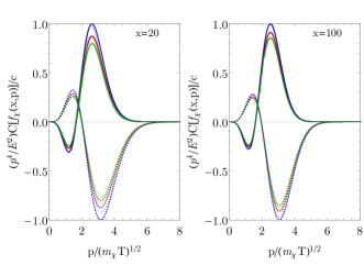
These results are compared to the corresponding Fokker-Planck approximation in Fig. 11 and Fig. 12, respectively. For low temperatures (right panels), as expected, the Fokker-Planck scattering term is always an excellent approximation. In the high-temperature regime (left panels), on the other hand, less separated scales (the momentum transfer scale $\sim T$ versus typical DM momenta $\sim\sqrt{m_{\chi}T_{\chi}}$) can become an issue for the Fokker-Planck approximation — especially if amplitudes support larger momentum transfers as, e.g., in the $|\mathcal{M}|^{2}_{\chi f\leftrightarrow\chi f}=-t/\Lambda^{2}$ example.

We conclude that the error induced when adopting the much simpler Fokker-Planck approximation, at temperatures relevant for chemical freeze-out, depends on the exact form of the scattering amplitude. The potential impact on the relic density in scenarios with early kinetic decoupling is therefore also unavoidably model-dependent. However, as for example in the threshold scenario discussed in Section 4.3, we expect that the dominant effect of early kinetic decoupling on the relic density can in many cases still be fairly well captured by the Fokker-Planck approximation.

B.2 Implementation

In discretized form, the full elastic collision term can be written as a linear operator of the form $C_{\text{el}}[f_{\chi}]/E=\hat{\mathbf{C}}_{\text{el}}\cdot\mathbf{f}$ with $\mathbf{f}=(f_{0},...,f_{N})^{T}$ being the momentum-discretized phase-space density $f_{\chi}$. The matrix $\hat{\mathbf{C}}_{\text{el}}$ can be written on a momentum grid, with $p,\tilde{p}\in\{p_{0},...,p_{N}\}$ and equal spacing $\Delta p$, as:

$$\hat{\mathbf{C}}_{\text{el}}=-\frac{\Delta p}{2\pi^{2}}\times$$ (36)

$$\begin{pmatrix}\sum\limits_{j\neq 0}^{N}\langle W\rangle_{0j}p_{j}^{2}e^{\beta(E_{0}-E_{j})/2}&-\langle W\rangle_{01}p_{1}^{2}e^{-\beta(E_{0}-E_{1})/2}&...\\ -\langle W\rangle_{10}{p_{0}}^{2}e^{-\beta(E_{1}-E_{0})/2}&\sum\limits_{j\neq 1}^{N}\langle W\rangle_{1j}p_{j}^{2}e^{\beta(E_{1}-E_{j})/2}&...\\ ...&...&...\end{pmatrix},$$

where $\beta\equiv 1/T$ and we introduced $\langle W\rangle_{ij}\equiv\langle W\rangle_{\tilde{\Omega}}(p_{i},p_{j},T)$ on the momentum grid. The routines returning the matrix in Eq. (36) needed for fBE, and its descretized second momentum moment needed for the cBE, have the internal DRAKE names GetScatMatrix and GetSecondMomentScat, respectively (see also Table 4).

For the sub-threshold annihilation case, these two routines can be found in the model file TH.wl, where Eq. (36) with $\langle W\rangle_{\tilde{\Omega}}$ as in Eq. (33) is implemented. To switch from the Fokker-Planck approximation to full $C_{\text{el}}$ in the cBE and fBE approaches, set FullCel=True in the setting file. These two routines can be adopted to other scattering scenarios, by replacing the $\langle W\rangle_{ij}$ dependent parts inside the routines.

References

- (1) Planck: N. Aghanim et. al., Planck 2018 results. VI. Cosmological parameters, Astron. Astrophys. 641 (2020) A6, [arXiv:1807.06209].
- (2) B. W. Lee and S. Weinberg, Cosmological Lower Bound on Heavy Neutrino Masses, Phys. Rev. Lett. 39 (1977) 165–168.
- (3) J. R. Ellis, J. S. Hagelin, D. V. Nanopoulos, K. A. Olive, and M. Srednicki, Supersymmetric Relics from the Big Bang, Nucl. Phys. B238 (1984) 453–476. [,223(1983)].
- (4) G. Jungman, M. Kamionkowski, and K. Griest, Supersymmetric dark matter, Phys. Rept. 267 (1996) 195–373, [hep-ph/9506380].
- (5) D. Hooper and S. Profumo, Dark Matter and Collider Phenomenology of Universal Extra Dimensions, Phys. Rept. 453 (2007) 29–115, [hep-ph/0701197].
- (6) G. Arcadi, M. Dutra, et. al., The waning of the WIMP? A review of models, searches, and constraints, Eur. Phys. J. C78 (2018) 203, [arXiv:1703.07364].
- (7) J. L. Feng and J. Kumar, The WIMPless Miracle: Dark-Matter Particles without Weak-Scale Masses or Weak Interactions, Phys. Rev. Lett. 101 (2008) 231301, [arXiv:0803.4196].
- (8) T. Bringmann, J. Edsjö, P. Gondolo, P. Ullio, and L. Bergström, DarkSUSY 6 : An Advanced Tool to Compute Dark Matter Properties Numerically, JCAP 07 (2018) 033, [arXiv:1802.03399].
- (9) F. Ambrogi, C. Arina, et. al., MadDM v.3.0: a Comprehensive Tool for Dark Matter Studies, Phys. Dark Univ. 24 (2019) 100249, [arXiv:1804.00044].
- (10) G. Belanger, F. Boudjema, A. Pukhov, and A. Semenov, MicrOMEGAs 2.0: A Program to calculate the relic density of dark matter in a generic model, Comput. Phys. Commun. 176 (2007) 367–382, [hep-ph/0607059].
- (11) A. Arbey and F. Mahmoudi, SuperIso Relic: A Program for calculating relic density and flavor physics observables in Supersymmetry, Comput. Phys. Commun. 181 (2010) 1277–1292, [arXiv:0906.0369].
- (12) L. Roszkowski, E. M. Sessolo, and A. J. Williams, What next for the CMSSM and the NUHM: Improved prospects for superpartner and dark matter detection, JHEP 08 (2014) 067, [arXiv:1405.4289].
- (13) P. Bechtle et. al., Killing the cMSSM softly, Eur. Phys. J. C 76 (2016) 96, [arXiv:1508.05951].
- (14) H. Baer, V. Barger, and H. Serce, SUSY under siege from direct and indirect WIMP detection experiments, Phys. Rev. D 94 (2016) 115019, [arXiv:1609.06735].
- (15) GAMBIT: P. Athron et. al., Global fits of GUT-scale SUSY models with GAMBIT, Eur. Phys. J. C 77 (2017) 824, [arXiv:1705.07935].
- (16) GAMBIT: P. Athron et. al., A global fit of the MSSM with GAMBIT, Eur. Phys. J. C 77 (2017) 879, [arXiv:1705.07917].
- (17) GAMBIT: P. Athron et. al., Status of the scalar singlet dark matter model, Eur. Phys. J. C 77 (2017) 568, [arXiv:1705.07931].
- (18) E. Bagnaschi et. al., Likelihood Analysis of the pMSSM11 in Light of LHC 13-TeV Data, Eur. Phys. J. C 78 (2018) 256, [arXiv:1710.11091].
- (19) J. C. Costa et. al., Likelihood Analysis of the Sub-GUT MSSM in Light of LHC 13-TeV Data, Eur. Phys. J. C 78 (2018) 158, [arXiv:1711.00458].
- (20) E. Bagnaschi et. al., Global Analysis of Dark Matter Simplified Models with Leptophobic Spin-One Mediators using MasterCode, Eur. Phys. J. C 79 (2019) 895, [arXiv:1905.00892].
- (21) P. Gondolo and G. Gelmini, Cosmic abundances of stable particles: Improved analysis, Nucl. Phys. B 360 (1991) 145–179.
- (22) J. Edsjö and P. Gondolo, Neutralino relic density including coannihilations, Phys. Rev. D 56 (1997) 1879–1894, [hep-ph/9704361].
- (23) K. Griest and D. Seckel, Three exceptions in the calculation of relic abundances, Phys. Rev. D 43 (1991) 3191–3203.
- (24) L. G. van den Aarssen, T. Bringmann, and Y. C. Goedecke, Thermal decoupling and the smallest subhalo mass in dark matter models with Sommerfeld-enhanced annihilation rates, Phys. Rev. D 85 (2012) 123512, [arXiv:1202.5456].
- (25) M. Duch and B. Grzadkowski, Resonance enhancement of dark matter interactions: the case for early kinetic decoupling and velocity dependent resonance width, JHEP 09 (2017) 159, [arXiv:1705.10777].
- (26) A. Kamada, H. J. Kim, H. Kim, and T. Sekiguchi, Self-Heating Dark Matter via Semiannihilation, Phys. Rev. Lett. 120 (2018) 131802, [arXiv:1707.09238].
- (27) A. Berlin, N. Blinov, S. Gori, P. Schuster, and N. Toro, Cosmology and Accelerator Tests of Strongly Interacting Dark Matter, Phys. Rev. D 97 (2018) 055033, [arXiv:1801.05805].
- (28) A. Kamada, H. J. Kim, and H. Kim, Self-heating of Strongly Interacting Massive Particles, Phys. Rev. D 98 (2018) 023509, [arXiv:1805.05648].
- (29) T. Abe, Effect of the early kinetic decoupling in a fermionic dark matter model, Phys. Rev. D 102 (2020) 035018, [arXiv:2004.10041].
- (30) T. Binder, T. Bringmann, M. Gustafsson, and A. Hryczuk, Early kinetic decoupling of dark matter: when the standard way of calculating the thermal relic density fails, Phys. Rev. D 96 (2017) 115010, [arXiv:1706.07433]. [Erratum: Phys.Rev.D 101, 099901 (2020)].
- (31) F. Brümmer, Coscattering in next-to-minimal dark matter and split supersymmetry, JHEP 01 (2020) 113, [arXiv:1910.01549].
- (32) K. Ala-Mattinen and K. Kainulainen, Precision calculations of dark matter relic abundance, JCAP 09 (2020) 040, [arXiv:1912.02870].
- (33) J. Bernstein, Kinetic Theory in the Expanding Universe. Cambridge Monographs on Mathematical Physics. Cambridge University Press, Cambridge, U.K., 1988.
- (34) E. W. Kolb and M. S. Turner, The Early Universe, vol. 69. 1990.
- (35) E. Bertschinger, The Effects of Cold Dark Matter Decoupling and Pair Annihilation on Cosmological Perturbations, Phys. Rev. D 74 (2006) 063509, [astro-ph/0607319].
- (36) T. Bringmann and S. Hofmann, Thermal decoupling of WIMPs from first principles, JCAP 0704 (2007) 016, [hep-ph/0612238]. [Erratum: JCAP1603,no.03,E02(2016)].
- (37) T. Bringmann, Particle Models and the Small-Scale Structure of Dark Matter, New J. Phys. 11 (2009) 105027, [arXiv:0903.0189].
- (38) T. Bringmann, H. T. Ihle, J. Kersten, and P. Walia, Suppressing structure formation at dwarf galaxy scales and below: late kinetic decoupling as a compelling alternative to warm dark matter, Phys. Rev. D94 (2016) 103529, [arXiv:1603.04884].
- (39) T. Binder, L. Covi, et. al., Matter Power Spectrum in Hidden Neutrino Interacting Dark Matter Models: A Closer Look at the Collision Term, JCAP 1611 (2016) 043, [arXiv:1602.07624].
- (40) J. Kasahara, Neutralino dark matter: the mass of the smallest halo and the golden region. PhD thesis, The University of Utah, 2009.
- (41) P. Gondolo, J. Hisano, and K. Kadota, The Effect of quark interactions on dark matter kinetic decoupling and the mass of the smallest dark halos, Phys. Rev. D86 (2012) 083523, [arXiv:1205.1914].
- (42) D. N. Spergel and P. J. Steinhardt, Observational evidence for selfinteracting cold dark matter, Phys. Rev. Lett. 84 (2000) 3760–3763, [astro-ph/9909386].
- (43) S. Tulin and H.-B. Yu, Dark Matter Self-interactions and Small Scale Structure, Phys. Rept. 730 (2018) 1–57, [arXiv:1705.02358].
- (44) W. E. Schiesser and G. W. Griffiths, A Compendium of Partial Differential Equation Models: Method of Lines Analysis with Matlab. Cambridge University Press, USA, 1 ed., 2009.
- (45) V. Silveira and A. Zee, SCALAR PHANTOMS, Phys. Lett. B161 (1985) 136–140.
- (46) J. McDonald, Gauge singlet scalars as cold dark matter, Phys. Rev. D50 (1994) 3637–3649, [hep-ph/0702143].
- (47) C. P. Burgess, M. Pospelov, and T. ter Veldhuis, The Minimal model of nonbaryonic dark matter: A Singlet scalar, Nucl. Phys. B619 (2001) 709–728, [hep-ph/0011335].
- (48) K. Atkinson, W. Han, and D. Stewart, Numerical Solution of Ordinary Differential Equations. 2009.
- (49) E. Anderson, Z. Bai, et. al., LAPACK Users’ Guide. Society for Industrial and Applied Mathematics, Philadelphia, PA, third ed., 1999.
- (50) L. F. Shampine and H. A. Watts, Depac - design of a user oriented package of ode solvers, .
- (51) A. Hektor, A. Hryczuk, and K. Kannike, Improved bounds on singlet dark matter, JHEP 03 (2019) 204, [arXiv:1901.08074].
- (52) J. L. Feng and J. Smolinsky, Impact of a resonance on thermal targets for invisible dark photon searches, Phys. Rev. D 96 (2017) 095022, [arXiv:1707.03835].
- (53) E. Bernreuther, S. Heeba, and F. Kahlhoefer, Resonant Sub-GeV Dirac Dark Matter, arXiv:2010.14522.
- (54) M. Fairbairn and J. Heal, Complementarity of dark matter searches at resonance, Phys. Rev. D 90 (2014) 115019, [arXiv:1406.3288].
- (55) G. Pozzo and Y. Zhang, Constraining resonant dark matter with combined LHC electroweakino searches, Phys. Lett. B 789 (2019) 582–591, [arXiv:1807.01476].
- (56) J. Hisano, S. Matsumoto, and M. M. Nojiri, Unitarity and higher order corrections in neutralino dark matter annihilation into two photons, Phys. Rev. D67 (2003) 075014, [hep-ph/0212022].
- (57) J. Hisano, S. Matsumoto, and M. M. Nojiri, Explosive dark matter annihilation, Phys. Rev. Lett. 92 (2004) 031303, [hep-ph/0307216].
- (58) J. Hisano, S. Matsumoto, M. M. Nojiri, and O. Saito, Non-perturbative effect on dark matter annihilation and gamma ray signature from galactic center, Phys. Rev. D71 (2005) 063528, [hep-ph/0412403].
- (59) J. Hisano, S. Matsumoto, M. Nagai, O. Saito, and M. Senami, Non-perturbative effect on thermal relic abundance of dark matter, Phys. Lett. B646 (2007) 34–38, [hep-ph/0610249].
- (60) M. Cirelli, A. Strumia, and M. Tamburini, Cosmology and Astrophysics of Minimal Dark Matter, Nucl. Phys. B787 (2007) 152–175, [arXiv:0706.4071].
- (61) A. Mitridate, M. Redi, J. Smirnov, and A. Strumia, Cosmological Implications of Dark Matter Bound States, JCAP 1705 (2017) 006, [arXiv:1702.01141].
- (62) J. B. Dent, S. Dutta, and R. J. Scherrer, Thermal Relic Abundances of Particles with Velocity-Dependent Interactions, Phys. Lett. B 687 (2010) 275–279, [arXiv:0909.4128].
- (63) J. Zavala, M. Vogelsberger, and S. D. White, Relic density and CMB constraints on dark matter annihilation with Sommerfeld enhancement, Phys. Rev. D 81 (2010) 083502, [arXiv:0910.5221].
- (64) J. L. Feng, M. Kaplinghat, and H.-B. Yu, Sommerfeld Enhancements for Thermal Relic Dark Matter, Phys. Rev. D 82 (2010) 083525, [arXiv:1005.4678].
- (65) S. Cassel, Sommerfeld factor for arbitrary partial wave processes, J. Phys. G 37 (2010) 105009, [arXiv:0903.5307].
- (66) T. R. Slatyer, The Sommerfeld enhancement for dark matter with an excited state, JCAP 02 (2010) 028, [arXiv:0910.5713].
- (67) M. Kawasaki, G. Steigman, and H.-S. Kang, Cosmological evolution of an early-decaying particle, Nuclear Physics B 403 (1993) 671 – 706.
- (68) T. Binder, M. Gustafsson, A. Kamada, S. M. R. Sandner, and M. Wiesner, Reannihilation of self-interacting dark matter, Phys. Rev. D 97 (2018) 123004, [arXiv:1712.01246].
- (69) R. T. D’Agnolo and J. T. Ruderman, Light Dark Matter from Forbidden Channels, Phys. Rev. Lett. 115 (2015) 061301, [arXiv:1505.07107].
- (70) T. Bringmann, F. Calore, A. Galea, and M. Garny, Electroweak and Higgs Boson Internal Bremsstrahlung: General considerations for Majorana dark matter annihilation and application to MSSM neutralinos, JHEP 09 (2017) 041, [arXiv:1705.03466].
- (71) E. Kuflik, M. Perelstein, N. R.-L. Lorier, and Y.-D. Tsai, Elastically Decoupling Dark Matter, Phys. Rev. Lett. 116 (2016) 221302, [arXiv:1512.04545].
- (72) E. Kuflik, M. Perelstein, N. R.-L. Lorier, and Y.-D. Tsai, Phenomenology of ELDER Dark Matter, JHEP 08 (2017) 078, [arXiv:1706.05381].
- (73) P. J. Fitzpatrick, H. Liu, T. R. Slatyer, and Y.-D. Tsai, New Pathways to the Relic Abundance of Vector-Portal Dark Matter, arXiv:2011.01240.
- (74) A. Biswas, S. Ganguly, and S. Roy, When Freeze-out occurs due to a non-Boltzmann suppression: A study of degenerate dark sector, arXiv:2011.02499.
- (75) D. Croon, G. Elor, R. Houtz, H. Murayama, and G. White, Light Dark Matter through Resonance Scanning, arXiv:2012.15284.
- (76) D. Boyanovsky and J. Wu, Small scale aspects of warm dark matter : power spectra and acoustic oscillations, Phys. Rev. D 83 (2011) 043524, [arXiv:1008.0992].
- (77) P. Hager and A. Kassiteridis, Phase-space Distribution Functions of Feebly Particles and Their Signatures, arXiv:2009.11308.
- (78) J. Lesgourgues and T. Tram, The Cosmic Linear Anisotropy Solving System (CLASS) IV: efficient implementation of non-cold relics, JCAP 09 (2011) 032, [arXiv:1104.2935].
- (79) M. Drees, F. Hajkarim, and E. R. Schmitz, The Effects of QCD Equation of State on the Relic Density of WIMP Dark Matter, JCAP 06 (2015) 025, [arXiv:1503.03513].
- (80) K. Saikawa and S. Shirai, Precise WIMP Dark Matter Abundance and Standard Model Thermodynamics, JCAP 08 (2020) 011, [arXiv:2005.03544].