Neural Production Systems

Abstract

Visual environments are structured, consisting of distinct objects or entities. These entities have properties—visible or latent—that determine the manner in which they interact with one another. To partition images into entities, deep-learning researchers have proposed structural inductive biases such as slot-based architectures. To model interactions among entities, equivariant graph neural nets (GNNs) are used, but these are not particularly well suited to the task for two reasons. First, GNNs do not predispose interactions to be sparse, as relationships among independent entities are likely to be. Second, GNNs do not factorize knowledge about interactions in an entity-conditional manner. As an alternative, we take inspiration from cognitive science and resurrect a classic approach, production systems, which consist of a set of rule templates that are applied by binding placeholder variables in the rules to specific entities. Rules are scored on their match to entities, and the best fitting rules are applied to update entity properties. In a series of experiments, we demonstrate that this architecture achieves a flexible, dynamic flow of control and serves to factorize entity-specific and rule-based information. This disentangling of knowledge achieves robust future-state prediction in rich visual environments, outperforming state-of-the-art methods using GNNs, and allows for the extrapolation from simple (few object) environments to more complex environments.

1 Introduction

Despite never having taken a physics course, every child beyond a young age appreciates that pushing a plate off the dining table will cause the plate to break. The laws of physics accurately characterize the dynamics of our natural world, and although explicit knowledge of these laws is not necessary to reason, we can reason explicitly about objects interacting through these laws. Humans can verbalize knowledge in propositional expressions such as “If a plate drops from table height, it will break,” and “If a video-game opponent approaches from behind and they are carrying a weapon, they are likely to attack you.” Expressing propositional knowledge is not a strength of current deep learning methods for several reasons. First, propositions are discrete and independent from one another. Second, propositions must be quantified in the manner of first-order logic; for example, the video-game proposition applies to any $X$ for which $X$ is an opponent and has a weapon. Incorporating the ability to express and reason about propositions should improve generalization in deep learning methods because this knowledge is modular— propositions can be formulated independently of each other— and can therefore be acquired incrementally. Propositions can also be composed with each other and applied consistently to all entities that match, yielding a powerful form of systematic generalization.

The classical AI literature from the 1980s can offer deep learning researchers a valuable perspective. In this era, reasoning, planning, and prediction were handled by architectures that performed propositional inference on symbolic knowledge representations. A simple example of such an architecture is the production system (Laird et al., 1986; Anderson, 1987), which expresses knowledge by condition-action rules. The rules operate on a working memory: rule conditions are matched to entities in working memory inspired by cognitive science, and such a match can trigger computational actions that update working memory or external actions that operate on the outside world.

Production systems were typically used to model high-level cognition, e.g., mathematical problem solving or procedure following; perception was not the focus of these models. It was assumed that the results of perception were placed into working memory in a symbolic form that could be operated on with the rules. In this article, we revisit production systems but from a deep learning perspective which naturally integrates perceptual processing and subsequent inference for visual reasoning problems. We describe an end-to-end deep learning model that constructs object-centric representations of entities in videos, and then operates on these entities with differentiable—and thus learnable—production rules. The essence of these rules, carried over from traditional symbolic system, is that they operate on variables that are bound, or linked, to the entities in the world. In the deep learning implementation, each production rule is represented by a distinct MLP with query-key attention mechanisms to specify the rule-entity binding and to determine when the rule should be triggered for a given entity. We are not the first to propose a neural instantiation of a production system architecture. Touretzky and Hinton (1988) gave a proof of principle that neural net hardware could be hardwired to implement a production system for symbolic reasoning; our work fundamentally differs from theirs in that (1) we focus on perceptual inference problems and (2) we use the architecture as an inductive bias for learning.

1.1 Variables and entities

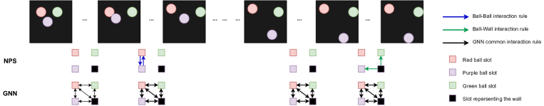
Figure 1: In this figure we show a visual comparison between NPS and dense architectures like GNNs. In NPS, a rule is only applied when an interaction takes place and it is applied only to the slots affected by the interaction. NPS also uses different rules for different kinds of interactions, while in GNN a common rule is applied to all slots irrespective of whether an interaction takes place or not (because of parameter sharing). Note the dynamic nature of the interaction graph in NPS, while in GNN, the graph is static.

What makes a rule general-purpose is that it incorporates placeholder variables that can be bound to arbitrary values or—the term we prefer in this article—entities. This notion of binding is familiar in functional programming languages, where these variables are called arguments. Analogously, the use of variables in the production rules we describe enable a model to reason about any set of entities that satisfy the selection criteria of the rule.

Consider a simple function in C like int add(int a, int b). This function binds its two integer operands to variables $a$ and $b$. The function does not apply if the operands are, say, character strings. The use of variables enables a programmer to reuse the same function to add any two integer values

In order for rules to operate on entities, these entities must be represented explicitly. That is, the visual world needs to be parsed in a task-relevant manner, e.g., distinguishing the sprites in a video game or the vehicles and pedestrians approaching an autonomous vehicle. Only in the past few years have deep learning vision researchers developed methods for object-centric representation (Le Roux et al., 2011; Eslami et al., 2016; Greff et al., 2016; Raposo et al., 2017; Van Steenkiste et al., 2018; Kosiorek et al., 2018; Engelcke et al., 2019; Burgess et al., 2019; Greff et al., 2019; Locatello et al., 2020a; Ahmed et al., 2020; Goyal et al., 2019; Zablotskaia et al., 2020; Rahaman et al., 2020; Du et al., 2020; Ding et al., 2020; Goyal et al., 2020; Ke et al., 2021). These methods differ in details but share the notion of a fixed number of slots (see Figure 1 for example), also known as object files, each encapsulating information about a single object. Importantly, the slots are interchangeable, meaning that it doesn’t matter if a scene with an apple and an orange encodes the apple in slot 1 and orange in slot 2 or vice-versa.

A model of visual reasoning must not only be able to represent entities but must also express knowledge about entity dynamics and interactions. To ensure systematic predictions, a model must be capable of applying knowledge to an entity regardless of the slot it is in and must be capable of applying the same knowledge to multiple instances of an entity. Several distinct approaches exist in the literature. The predominant approach uses graph neural networks to model slot-to-slot interactions (Scarselli et al., 2008; Bronstein et al., 2017; Watters et al., 2017; Van Steenkiste et al., 2018; Kipf et al., 2018; Battaglia et al., 2018; Tacchetti et al., 2018). To ensure systematicity, the GNN must share parameters among the edges. In a recent article, Goyal et al. (2020) developed a more general framework in which parameters are shared but slots can dynamically select which parameters to use in a state-dependent manner. Each set of parameters is referred to as a schema, and slots use a query-key attention mechanism to select which schema to apply at each time step. Multiple slots can select the same schema. In both GNNs and SCOFF, modeling dynamics involves each slot interacting with each other slot. In the work we describe in this article, we replace the direct slot-to-slot interactions with rules, which mediate sparse interactions among slots (See arrows in Figure 1).

Thus our main contribution is that we introduce NPS, which offers a way to model dynamic and sparse interactions among the variables in a graph and also allows dynamic sharing of multiple sets of parameters among these interactions. Most architectures used for modelling interactions in the current literature use statically instantiated graph which model all possible interactions for a given variable at each step i.e. dense interactions. Also such dense architectures share a single set of parameters across all interactions which maybe quite restrictive in terms of representational capacity. A visual comparison between these two kinds of architectures is shown in Figure 1. Through our experiments we show the advantage of modeling interactions in the proposed manner using NPS in visually rich physical environments. We also show that our method results in an intuitive factorization of rules and entities.

2 Production System

Formally, our notion of a production system consists of a set of entities and a set of rules, along with a mechanism for selecting rules to apply on subsets of the entities. Implicit in a rule is a specification of the properties of relevant entities, e.g., a rule might apply to one type of sprite in a video game but not another. The control flow of a production system dynamically selects rules as well as bindings between rules and entities, allowing different rules to be chosen and different entities to be manipulated at each point in time.

The neural production system we describe shares essential properties with traditional production system, particularly with regard to the compositionality and generality of the knowledge they embody. Lovett and Anderson (2005) describe four desirable properties commonly attributed to symbolic systems that apply to our work as well.

Production rules are modular. Each production rule represents a unit of knowledge and are atomic such that any production rule can be intervened (added, modified or deleted) independently of other production rules in the system.

Production rules are abstract. Production rules allow for generalization because their conditions may be represented as high-level abstract knowledge that match to a wide range of patterns. These conditions specify the attributes of relationship(s) between entities without specifying the entities themselves. The ability to represent abstract knowledge allows for the transfer of learning across different environments as long as they fit within the conditions of the given production rule.

Production rules are sparse. In order that production rules have broad applicability, they involve only a subset of entities. This assumption imposes a strong prior that dependencies among entities are sparse. In the context of visual reasoning, we conjecture that this prior is superior to what has often been assumed in the past, particularly in the disentanglement literature—independence among entities Higgins et al. (2016); Chen et al. (2018).

Production rules represent causal knowledge and are thus asymmetric. Each rule can be decomposed into a {condition, action} pair, where the action reflects a state change that is a causal consequence of the conditions being met.

These four properties are sufficient conditions for knowledge to be expressed in production rule form. These properties specify how knowledge is represented, but not what knowledge is represented. The latter is inferred by learning mechanisms under the inductive bias provided by the form of production rules.

3 Neural Production System: Slots and Sparse Rules

The Neural Production System (NPS), illustrated in Figure 2, provides an architectural backbone that supports the detection and inference of entity (object) representations in an input sequence, and the underlying rules which govern the interactions between these entities in time and space. The input sequence indexed by time step $t$, $\{{\bm{x}}^{1},\ldots,{\bm{x}}^{t},\ldots,{\bm{x}}^{T}\}$, for instance the frames in a video, are processed by a neural encoder (Burgess et al., 2019; Greff et al., 2019; Goyal et al., 2019, 2020) applied to each ${\bm{x}}^{t}$, to obtain a set of $M$ entity representations $\{{\bm{V}}_{1}^{t},\ldots,\ldots,{\bm{V}}_{M}^{t}\}$, one for each of the $M$ slots. These representations describe an entity and are updated based on both the previous state, ${\bm{V}}^{t-1}$ and the current input, ${\bm{x}}^{t}$.

NPS consists of $N$ separately encoded rules, $\{\bm{R}_{1},\bm{R}_{2},..,\bm{R}_{N}\}$. Each rule consists of two components, $\bm{R}_{i}=(\vec{\bm{R}_{i}},MLP_{i})$, where $\vec{\bm{R}_{i}}$ is a learned rule embedding vector, which can be thought of as a template defining the condition for when a rule applies; and $MLP_{i}$, which determines the action taken by a rule. Both $\vec{\bm{R}_{i}}$ and the parameters of $MLP_{i}$ are learned along with the other parameters of the model using back-propagation on an objective optimized end-to-end.

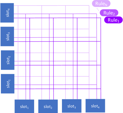
Figure 2: Rule and slot combinatorics. Condition-action rules specify how entities interact. Slots maintain the time-varying state of an entity. Every rule is matched to every pair of slots. Through key-value attention, a goodness of match is determined, and a rule is selected along with its binding to slots.

In the general form of the model, each slot selects a rule that will be applied to it to change its state. This can potentially be performed several times, with possibly different rules applied at each step. Rule selection is done using an attention mechanism described in detail below. Each rule specifies conditions and actions on a pair of slots. Therefore, while modifying the state of a slot using a rule, it can take the state of another slot into account. The slot which is being modified is called the primary slot and other is called the contextual slot. The contextual slot is also selected using an attention mechanism described in detail below.

3.1 Computational Steps in NPS

In this section, we give a detailed description of the rule selection and application procedure for the slots. First, we will formalize the definitions of a few terms that we will use to explain our method. We use the term primary slot to refer to slot ${\bm{V}}_{p}$ whose state gets modified by a rule $\bm{R}_{r}$. We use the term contextual slot to refer to the slot ${\bm{V}}_{c}$ that the rule $\bm{R}_{r}$ takes into account while modifying the state of the primary slot ${\bm{V}}_{p}$.

Notation. We consider a set of ${\bm{N}}$ rules $\{\bm{R}_{1},\bm{R}_{2},\ldots,\bm{R}_{N}\}$ and a set of ${\bm{T}}$ input frames $\{{\bm{x}}^{1},{\bm{x}}^{2},\ldots,{\bm{x}}^{T}\}$. Each frame ${\bm{x}}^{t}$ is encoded into a set of ${\bm{M}}$ slots $\{{\bm{V}}^{t}_{1},{\bm{V}}^{t}_{2},\ldots,{\bm{V}}^{t}_{M}\}$. In the following discussion, we omit the index over ${\bm{t}}$ for simplicity.

Step 1. is external to NPS and involves parsing an input image, ${\bm{x}}^{t}$, into slot-based entities conditioned on the previous state of the slot-based entities. Any of the methods proposed in the literature to obtain a slot-wise representation of entities can be used (Burgess et al., 2019; Greff et al., 2019; Goyal et al., 2019, 2020). The next three steps constitute the rule selection and application procedure.

Step 2. For each primary slot ${\bm{V}}_{p}$, we attend to a rule $\bm{R}_{r}$ to be applied. Here, the queries come from the primary slot: ${\bm{q}}_{p}={\bm{V}}_{p}W^{q}$, and the keys come from the rules: ${\bm{k}}_{i}=\vec{R_{i}}W^{k}\quad\forall{\bm{i}}\in\{1,\ldots,{\bm{N}}\}$. The rule is selected using a straight-through Gumbel softmax (Jang et al., 2016) to achieve a learnable hard decision: ${\bm{r}}=\mathrm{argmax}_{i}({\bm{q}}_{p}{\bm{k}}_{i}+\gamma),\text{ where }\gamma\sim\mathrm{Gumbel}(0,1)$. This competition is a noisy version of rule matching and prioritization in traditional production systems.

Step 3. For a given primary slot ${\bm{V}}_{p}$ and selected rule $\bm{R}_{r}$, a contextual slot ${\bm{V}}_{c}$ is selected using another attention mechanism. In this case the query comes from the primary slot: ${\bm{q}}_{p}={\bm{V}}_{p}W^{q}$, and the keys from all the slots: ${\bm{k}}_{j}={\bm{V}}_{j}W^{q}\quad\forall{\bm{j}}\in\{1,\ldots,{\bm{M}}\}$. The selection takes place using a straight-through Gumbel softmax similar to step 2: ${\bm{c}}=\mathrm{argmax}_{j}({\bm{q}}_{p}{\bm{k}}_{j}+\gamma),\text{ where }\gamma\sim\mathrm{Gumbel}(0,1)$. Note that each rule application is sparse since it takes into account only 1 contextual slot for modifying a primary slot, while other methods like GNNs take into account all slots for modifying a primary slot.

Step 4. Rule Application: the selected rule $\bm{R}_{r}$ is applied to the primary slot ${\bm{V}}_{p}$ based on the rule and the current contents of the primary and contextual slots. The rule-specific $MLP_{{r}}$, takes as input the concatenated representation of the state of the primary and contextual slots, ${\bm{V}}_{{p}}$ and ${\bm{V}}_{{c}}$, and produces an output, which is then used to change the state of the primary slot ${\bm{V}}_{{p}}$ by residual addition.

3.2 Rule Application: Sequential vs Parallel Rule Application

In the previous section, we have described how each rule application only considers another contextual slot for the given primary slot i.e., contextual sparsity. We can also consider application sparsity, wherein we use the rules to update the states of only a subset of the slots. In this scenario, only the selected slots would be primary slots. This setting will be helpful when there is an entity in an environment that is stationary, or it is following its own default dynamics unaffected by other entities. Therefore, it does not need to consider other entities to update its state. We explore two scenarios for enabling application sparsity.

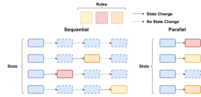
Figure 3: This figure demonstrates the sequential and parallel rule application.

Parallel Rule Application. Each of the $M$ slots selects a rule to potentially change its state. To enable sparse changes, we provide an extra Null Rule in addition to the available $N$ rules. If a slot picks the null rule in step 2 of the above procedure, we do not update its state.

Sequential Rule Application. In this setting, only one slot gets updated in each rule application step. Therefore, only one slot is selected as the primary slot. This can be facilitated by modifying step 2 above to select one {primary slot, rule} pair among ${\bm{N}}{\bm{M}}$ {rule, slot} pairs. The queries come from each slot: ${\bm{q}}_{j}={\bm{V}}_{j}W^{q}\quad\forall{\bm{j}}\in\{1,\ldots,{\bm{M}}\}$, the keys come from the rules: ${\bm{k}}_{i}=R_{i}W^{k}\quad\forall{\bm{i}}\in\{1,\ldots,{\bm{N}}\}$. The straight-through Gumbel softmax selects one (primary slot, rule) pair: ${\bm{p}},{\bm{r}}=\mathrm{argmax}_{i,j}({\bm{q}}_{p}{\bm{k}}_{i}+\gamma),\text{ where }\gamma\sim\mathrm{Gumbel}(0,1)$. In the sequential regime, we allow the rule application procedure (step 2, 3, 4 above) to be performed multiple times iteratively in $K$ rule application stages for each time-step $t$.

A pictorial demonstration of both rule application regimes can be found in Figure 3. We provide detailed algorithms for the sequential and parallel regimes in Appendix.

4 Experiments

Table 1: This table shows the segregation of rules for the MNIST Transformation task. Each cell indicates the number of times the corresponding rule is used for the given operation. We can see that NPS automatically and perfectly learns a separate rule for each operation.

	Rule 1	Rule 2	Rule 3	Rule 4
Translate Down	5039	0	0	0
Translate Up	0	4950	0	0
Rotate Right	0	0	5030	0
Rotate Left	0	0	0	4981

We demonstrate the effectiveness of NPS on multiple tasks and compare to a comprehensive set of baselines. To show that NPS can learn intuitive rules from the data generating distribution, we design a couple of simple toy experiments with well-defined discrete operations. Results show that NPS can accurately recover each operation defined by the data and learn to represent each operation using a separate rule. We then move to a much more complicated and visually rich setting with abstract physical rules and show that factorization of knowledge into rules as offered by NPS does scale up to such settings. We study and compare the parallel and sequential rule application procedures and try to understand the settings which favour each. We then evaluate the benefits of reusable, dynamic and sparse interactions as offered by NPS in a wide variety of physical environments by comparing it against various baselines. We conduct ablation studies to assess the contribution of different components of NPS. Here we briefly outline the tasks considered and direct the reader to the Appendix for full details on each task and details on hyperparameter settings.

Discussion of baselines. NPS is an interaction network, therefore we use other widely used interaction networks such as multihead attention and graph neural networks (Goyal et al. (2019), Goyal et al. (2020), Veerapaneni et al. (2019), Kipf et al. (2019)) for comparison. Goyal et al. (2019) and Goyal et al. (2020) use an attention based interaction network to capture interactions between the slots, while Veerapaneni et al. (2019) and Kipf et al. (2019) use a GNN based interaction network. We also consider the recently introduced convolutional interaction network (CIN) (Qi et al., 2021) which captures dense pairwise interactions like GNN but uses a convolutional network instead of MLPs to better utilize spatial information. The proposed method, similar to other interaction networks, is agnostic to the encoder backbone used to encode the input image into slots, therefore we compare NPS to other interaction networks across a wide-variety of encoder backbones.

4.1 Learning intuitive rules with NPS: Toy Simulations

We designed a couple of simple tasks with well-defined discrete rules to show that NPS can learn intuitive and interpretable rules. We also show the efficiency and effectiveness of the selection procedure (step 2 and step 3 in section 3.1) by comparing against a baseline with many more parameters. Both tasks require a single modification of only one of the available entities, therefore the use of sequential or parallel rule application would not make a difference here since parallel rule application in which all-but-one slots select the null rule is similar to sequential rule application with 1 rule application step. To simplify the presentation, we describe the setup for both tasks using the sequential rule application procedure.

MNIST Transformation. We test whether NPS  can learn simple rules for performing transformations on MNIST digits. We generate data with four transformations: {Translate Up, Translate Down, Rotate Right, Rotate Left}. We feed the input image (${\bm{X}}$) and the transformation (${\bm{o}}$) to be performed as a one-hot vector to the model. The detailed setup is described in Appendix. For this task, we evaluate whether NPS can learn to use a unique rule for each transformation.

We use 4 rules corresponding to the 4 transformations with the hope that the correct transformations are recovered. Indeed, we observe that NPS  successfully learns to represent each transformation using a separate rule as shown in Table 1. Our model achieves an MSE of 0.02. A visualization of the outputs from our model and further details can be found in Appendix C.

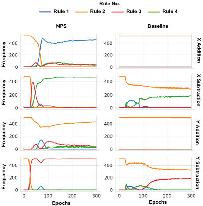
Figure 4: Coordinate Arithmetic Task. Here, we compare NPS to the baseline model in terms of segregation of rules as the training progresses. X-axis shows the epochs and Y-axis shows the frequency with which Rule $i$ is used for the given operation. We can see that NPS disentangles the operations perfectly as training progresses with a unique rule specializing to every operation while the baseline model fails to do so.

Coordinate Arithmetic Task. The model is tasked with performing arithmetic operations on 2D coordinates. Given $(X_{0},Y_{0})$ and $(X_{1},Y_{1})$, we can apply the following operations: {X Addition: $(X_{r},Y_{r})=(X_{0}+X_{1},Y_{0})$, X Subtraction: $(X_{r},Y_{r})=(X_{0}-X_{1},Y_{0})$, Y Addition: $(X_{r},Y_{r})=(X_{0},Y_{0}+Y_{1})$, Y Subtraction: ${X_{r},Y_{r}}=(X_{0},Y_{0}-Y_{1})$}, where $(X_{r},Y_{r})$ is the resultant coordinate.

In this task, the model is given 2 input coordinates $X=[(x_{i},y_{i}),(x_{j},y_{j})]$ and the expected output coordinates $Y=[(\hat{x_{i}},\hat{y_{i}}),(\hat{x_{j}},\hat{y_{j}})]$ . The model is supposed to infer the correct rule to produce the correct output coordinates. During data collection, the true output is obtained by performing a random transformation on a randomly selected coordinate in $X$ (primary coordinate), taking another randomly selected coordinate from $X$ (contextual coordinate) into account. The detailed setup is described in Appendix D. We use an NPS model with 4 rules for this task. We use the the selection procedure in step 2 and step 3 of algorithm 1 to select the primary coordinate, contextual coordinate, and the rule. For the baseline we replace the selection procedure in NPS (i.e. step 2 and step 3 in algorithm 1) with a routing MLP similar to Fedus et al. (2021).

This routing MLP has 3 heads (one each for selecting the primary coordinate, contextual coordinate, and the rule). The baseline has 4 times more parameters than NPS. The final output is produced by the rule MLP which does not have access to the true output, hence the model cannot simply copy the true output to produce the actual output. Unlike the MNIST transformation task, we do not provide the operation to be performed as a one-hot vector input to the model, therefore it needs to infer the available operations from the data demonstrations.

Table 2: This table shows segregation of rules when we use NPS with 5 rules but the data generation distributions describes only 4 possible operations. We can see that only 4 rules get majorly utilized thus confirming that NPS successfully recovers all possible operations described by the data.

	Rule 1	Rule 2	Rule 3	Rule 4	Rule 5
X Addition	360	99	45	13	0
X Subtraction	0	482	0	1	0
Y Subtraction	0	39	453	2	0
Y Addition	0	57	15	99	335

We show the segregation of rules for NPS and the baseline in Figure 4. We can see that NPS learns to use a unique rule for each operation while the baseline struggles to disentangle the underlying operations properly. NPS also outperforms the baseline in terms of MSE achieving an MSE of 0.01_$\pm$0.001 while the baseline achieves an MSE of 0.04_$\pm$0.008. To further confirm that NPS learns all the available operations correctly from raw data demonstrations, we use an NPS model with 5 rules. We expect that in this case NPS should utilize only 4 rules since the data describes only 4 unique operations and indeed we observe that NPS ends up mostly utilizing 4 of the available 5 rules as shown in Table 2.

4.2 Parallel vs Sequential Rule Application

We compare the parallel and sequential rule application procedures, to understand the settings that favour one or the other, over two tasks: (1) Bouncing Balls, (2) Shapes Stack. We use the term PNPS to refer to parallel rule application and SNPS to refer to sequential rule application.

Model Name	Test	Transfer
RPIN (Qi et al. (2021))	1.254$\pm$0.008	6.377$\pm$0.325
PNPS	1.250$\pm$0.007	5.411$\pm$0.45
SNPS	1.68$\pm$0.02	5.80$\pm$0.15

Table 3: Prediction error of the compared models on the shapes stack dataset (lower is better) for the test as well as transfer setting. In the test setting the number of rollout steps ${\bm{t}}$ is set to 15 and in the transfer setting it is set to 30. We can see that PNPS outperforms the RPIN baseline in both the test and transfer setting while SNPS fails to do so. Results across 15 seeds.

Shapes Stack.

We use the shapes stack dataset introduced by Groth et al. (2018). This dataset consists of objects stacked on top of each other as shown in Figure 5. These objects fall under the influence of gravity. For our experiments, We follow the same setup as Qi et al. (2021). In this task, given the first frame, the model is tasked with predicting the object bounding boxes for the next ${\bm{t}}$ timesteps. The first frame is encoded using a convolutional network followed by RoIPooling (Girshick (2015)) to extract object-centric visual features. The object-centric features are then passed to the dynamics model to predict object bounding boxes of the next ${\bm{t}}$ steps. Qi et al. (2021) propose a Region Proposal Interaction Network (RPIN) to solve this task. The dynamics model in RPIN consists of an Interaction Network proposed in Battaglia et al. (2016). To better utilize spatial information, Qi et al. (2021) propose an extension of the interaction operators in interaction net to operate on 3D tensors. This is achieved by replacing the MLP operations in the original interaction networks with convolutions. They call this new network Convolutional Interaction Network (CIN). For the proposed model, we replace this CIN in RPIN by NPS. To ensure a fair comparison to CIN, we use CNNs to represent rules in NPS instead of MLPs. CIN captures all pairwise interactions between objects using a convolutional network. In NPS, we capture sparse interactions (contextual sparsity) as compared to dense pairwise interactions captured by CIN. Also, in NPS we update only a few subset of slots per step instead of all slots (application sparsity).

We consider two evaluation settings. (1) Test setting: The number of rollout timesteps is same as that seen during training (i.e. ${\bm{t}}=15$); (2) Transfer Setting: The number of rollout timesteps is higher than that seen during training (i.e. ${\bm{t}}=30$).

We present our results on the shapes stack dataset in Table 3. We can see that both PNPS and SNPS outperform the baseline RPIN in the transfer setting, while only PNPS outperforms the baseline in the test setting and SNPS fails to do so. We can see that PNPS outperforms SNPS. We attribute this to the reduced application sparsity with PNPS, i.e., it is more likely that the state of a slot gets updated in PNPS as compared to SNPS. For instance, consider an NPS model with ${\bm{N}}$ uniformly chosen rules and ${\bm{M}}$ slots. The probability that the state of a slot gets updated in PNPS is $P_{PNPS}={\bm{N}}-1/{\bm{N}}$ (since 1 rule is the null rule), while the same probability for SNPS is $P_{SNPS}=1/{\bm{M}}$ (since only 1 slot gets updated per rule application step).

For this task, we run both PNPS and SNPS for ${\bm{N}}=\{1,2,4,6\}$ rules and ${\bm{M}}=3$. For any given ${\bm{N}}$, we observe that $P_{PNPS}>P_{SNPS}$. Even when we have multiple rule application steps in SNPS, it might end up selecting the same slot to be updated in more than one of these steps. We report the best performance obtained for PNPS and SNPS across all ${\bm{N}}$, which is ${\bm{N}}=\{2+1\quad\text{Null Rule}\}$ for PNPS and ${\bm{N}}=4$ for SNPS, in Table 3. Shapes stack is a dataset that would prefer a model with less application sparsity since all the objects are tightly bound to each other (objects are placed on top of each other), therefore all objects spend the majority of their time interacting with the objects directly above or below them. We attribute the higher performance of PNPS compared to RPIN to the higher contextual sparsity of PNPS. Each example in the shapes stack task consists of 3 objects. Even though the blocks are tightly bound to each other, each block is only affected by the objects it is in direct contact with. For example, the top-most object is only affected by the object directly below it. The contextual sparsity offered by PNPS is a strong inductive bias to model such sparse interactions while RPIN models all pairwise interactions between the objects. Figure 5 shows an intuitive illustration of the PNPS model for the shapes stack dataset. In the figure, Rule 2 actually refers to the Null Rule, while Rule 1 refers to all the other non-null rules. The bottom-most block picks the Null Rule most times, as the bottom-most block generally does not move.

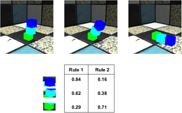
Figure 5: Here we show the rule selection statistics from the proposed model for all entities in the shapes stack dataset across all examples. Each example contains 3 entities as shown above. Each cell in the table shows the probability with which the given rule is triggered for the corresponding entity. We can see that the bottom-most entity triggers rule 2 most of the time while the other 2 entities trigger rule 1 most often. This is quite intuitive as, for most examples, the bottom-most entity remains static and does not move at all while the upper entities fall. Therefore, rule 2 captures information which is relevant to static entities, while rule 1 captures physical rules relevant to the interactions and motion of the upper entities.

Bouncing Balls.

We consider a bouncing-balls environment in which multiple balls move with billiard-ball dynamics. We validate our model on a colored version of this dataset. This is a next-step prediction task in which the model is tasked with predicting the final binary mask of each ball. We compare the following methods: (a) SCOFF (Goyal et al., 2020): factorization of knowledge in terms of slots (object properties) and schemata, the latter capturing object dynamics; (b) SCOFF++: we extend SCOFF by using the idea of iterative competition as proposed in slot attention (SA) (Locatello et al., 2020a); SCOFF + PNPS/SNPS: We replace pairwise slot-to-slot interaction in SCOFF++ with parallel or sequential rule application. For comparing different methods, we use the Adjusted Rand Index or ARI (Rand, 1971). To investigate how the factorization in the form of rules allows for extrapolating knowledge from fewer to more objects, we increase the number of objects from 4 during training to 6-8 during testing.

We present the results of our experiments in Table 4. Contrary to the shapes stack task, we see that SNPS outperforms PNPS for the bouncing balls task. The balls are not tightly bound together into a single tower as in the shapes stack. Most of the time, a single ball follows its own dynamics, only occasionally interacting with another ball. Rules in NPS capture interaction dynamics between entities, hence they would only be required to change the state of an entity when it interacts with another entity. In the case of bouncing balls, this interaction takes place through a collision between multiple balls. Since for a single ball, such collisions are rare, SNPS, which has higher application sparsity (less probability of modifying the state of an entity), performs better as compared to PNPS (lower application sparsity). Also note that, SNPS has the ability to compose multiple rules together by virtue of having multiple rule application stages. A visualization of the rule and entity selections by the proposed algorithm can be found in Appendix Figure 9.

Given the analysis in this section, we can conclude that PNPS is expected to work better when interactions among entities are more frequent while SNPS is expected to work better when interactions are rare and most of the time, each entity follows its own dynamics. Note that, for both SNPS and PNPS, the rule application considers only 1 other entity as context. Therefore, both approaches have equal contextual sparsity while the baselines that we consider (SCOFF and RPIN) capture dense pairwise interactions. We discuss the benefits of contextual sparsity in more detail in the next section. More details regarding our setup for the above experiments can be found in Appendix.

4.3 Benefits of Sparse Interactions Offered by NPS

In NPS, one can view the computational graph as a dynamically constructed GNN resulting from applying dynamically selected rules, where the states of the slots are represented on the different nodes of the graph, and different rules dynamically instantiate an hyper-edge between a set of slots (the primary slot and the contextual slot). It is important to emphasize that the topology of the graph induced in NPS is dynamic and sparse (only a few nodes affected), while in most GNNs the topology is fixed and dense (all nodes affected). In this section, through a thorough set of experiments, we show that learning sparse and dynamic interactions using NPS indeed works better for the problems we consider than learning dense interactions using GNNs. We consider two types of tasks: (1) Learning Action Conditioned World Models (2) Physical Reasoning. We use SNPS for all these experiments since in the environments that we consider here, interactions among entities are rare.

Model Name	Test	Transfer
SCOFF	0.28	0.15
SCOFF++	0.8437	0.2632
PNPS (10 Rules+1 Null Rule)	0.7813	0.1997
SNPS (10 Rules)	0.8518	0.3553

Table 4: Here we show the ARI achieved by the models on the bouncing balls dataset (higher is better). We can see that SNPS outperforms SCOFF and SCOFF++ while PNPS has a poor performance in this task. Results average across 2 seeds.

Learning Action-Conditioned World Models.

For learning action-conditioned world models, we follow the same experimental setup as Kipf et al. (2019). Therefore, all the tasks in this section are next-$K$ step ($K=\{1,5,10\}$) prediction tasks, given the intermediate actions, and with the predictions being performed in the latent space. We use the Hits at Rank 1 (H@1) metrics described by Kipf et al. (2019) for evaluation. H@1 is 1 for a particular example if the predicted state representation is nearest to the encoded true observation and 0 otherwise. We report the average of this score over the test set (higher is better).

Physics Environment.

The physics environment (Ke et al., 2021) simulates a simple physical world. It consists of blocks of unique but unknown weights. The dynamics for the interaction between blocks is that the movement of heavier blocks pushes lighter blocks on their path. This rule creates an acyclic causal graph between the blocks. For an accurate world model, the learner needs to infer the correct weights through demonstrations. Interactions in this environment are sparse and only involve two blocks at a time, therefore we expect NPS to outperform dense architectures like GNNs. This environment is demonstrated in Appendix Fig 11.

We follow the same setup as Kipf et al. (2019). We use their C-SWM model as baseline. For the proposed model, we only replace the GNN from C-SWM by NPS. GNNs generally share parameters across edges, but in NPS each rule has separate parameters. For a fair comparison to GNN, we use an NPS model with 1 rule. Note that this setting is still different from GNNs as in GNNs at each step every slot is updated by instantiating edges between all pairs of slots, while in NPS an edge is dynamically instantiated between a single pair of slots and only the state of the selected slot (i.e., primary slot) gets updated.

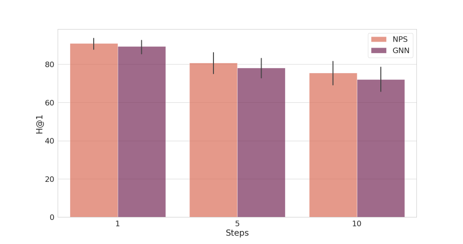
(a) Physics Env

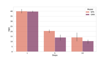
(b) Atari Games

Figure 6: Action-Conditioned World Models, with number of future steps to be predicted for the world-model on the horizontal axes. (a) Here we show a comparison between GNNs and the proposed NPS on the physics environment using the H@1 metric (higher is better). (b) Comparison of average H@1 scores across 5 Atari games for the proposed model NPS and GNN.

The results of our experiments are presented in Figure 6(a). We can see that NPS outperforms GNNs for all rollouts. Multi-step settings are more difficult to model as errors may get compounded over time steps. The sparsity of NPS (only a single slot affected per step) reduces compounding of errors and enhances symmetry-breaking in the assignment of transformations to rules, while in the case of GNNs, since all entities are affected per step, there is a higher possibility of errors getting compounded. We can see that even with a single rule, we significantly outperform GNNs thus proving the effectiveness of dynamically instantiating edges between entities.

Atari Games.

We also test the proposed model in the more complicated setting of Atari. Atari games also have sparse interactions between entities. For instance, in Pong, any interaction involves only 2 entities: (1) paddle and ball or (2) ball and the wall. Therefore, we expect sparse interactions captured by NPS to outperform GNNs here as well.

We follow the same setup as for the physics environment described in the previous section. We present the results for the Atari experiments in Figure 6(b), showing the average H@1 score across 5 games: Pong, Space Invaders, Freeway, Breakout, and QBert. As expected, we can see that the proposed model achieves a higher score than the GNN-based C-SWM. The results for the Atari experiments reinforce the claim that NPS is especially good at learning sparse interactions.

Learning Rules for Physical Reasoning.

To show the effectiveness of the proposed approach for physical reasoning tasks, we evaluate NPS on another dataset: Sprites-MOT (He et al., 2018). The Sprites-MOT dataset was introduced by He et al. (2018). The dataset contains a set of moving objects of various shapes. This dataset aims to test whether a model can handle occlusions correctly. Each frame has consistent bounding boxes which may cause the objects to appear or disappear from the scene. A model which performs well should be able to track the motion of all objects irrespective of whether they are occluded or not. We follow the same setup as Weis et al. (2020). We use the OP3 model (Veerapaneni et al., 2019) as our baseline. To test the proposed model, we replace the GNN-based transition model in OP3 with the proposed NPS.

Model	MOTA $\uparrow$	MOTP $\uparrow$
OP3	89.1$\pm$5.1	78.4$\pm$2.4
NPS	90.72$\pm$5.15	79.91$\pm$0.3

Table 5: Sprites-MOT. Comparison between the proposed NPS and the baseline OP3 using the MOTA and MOTP metrics on the sprites-MOT dataset ($\uparrow$: higher is better). Average over 3 random seeds.

We use the same evaluation protocol as followed by Weis et al. (2020) which is based on the MOT (Multi-object tracking) challenge (Milan et al., 2016). The results on the MOTA and MOTP metrics for this task are presented in Table 5. The results on the other metrics are presented in appendix Table 10. We ask the reader to refer to appendix F.1 for more details about these metrics. We can see that for almost all metrics, NPS outperforms the OP3 baseline. Although this dataset does not contain physical interactions between the objects, sparse rule application should still be useful in dealing with occlusions. At any time step, only a single object is affected by occlusions i.e., it may get occluded due to another object or due to a prespecified bounding box, while the other objects follow their default dynamics. Therefore, a rule should be applied to only the object (or entity) affected (i.e., not visible) due to occlusion and may take into account any other object or entity that is responsible for the occlusion.

5 Discussion and Conclusion

For AI agents such as robots trying to make sense of their environment, the only observables are low-level variables like pixels in images. To generalize well, an agent must induce high-level entities as well as discover and disentangle the rules that govern how these entities actually interact with each other. Here we have focused on perceptual inference problems and proposed NPS, a neural instantiation of production systems by introducing an important inductive bias in the architecture following the proposals of Marcus (2003); Bengio (2017); Goyal and Bengio (2020); Ke et al. (2021).

Limitations & Looking Forward. Our experiments highlight the advantages brought by the factorization of knowledge into a small set of entities and sparse sequentially applied rules. Immediate future work would investigate how to take advantage of these inductive biases for more complex physical environments (Ahmed et al., 2020) and novel planning methods, which might be more sample efficient than standard ones (Schrittwieser et al., 2020).

We also find that Sequential and Parallel NPS have different properties suited towards different domains. Future work should explore how to effectively combine these two approaches. We discuss this in more detail in Appendix section E.3.

6 Acknowledgements

The authors would also like to thank Alex Lamb, Stefan Bauer, Nicolas Chapados, Danilo Rezende, Matthew Botvinick and Kelsey Allen for brainstorming sessions. We are also thankful to Dianbo Liu, Damjan Kalajdzievski and Osama Ahmed for proofreading. We would like to thank Samsung Electronics Co. Ltd. and CIFAR for funding this research. We would also like to thank Google for providing Google cloud credits used in this work.

Appendix

Algorithm 1 Sequential Neural Production System model

0:  

  Input: Input sequence $\{{\bm{x}}^{1},\ldots,{\bm{x}}^{t},\ldots,{\bm{x}}^{T}\}$, set of embeddings describing the rules $\vec{\bm{R}_{i}}$, and set of MLPs $(MLP_{i})$ corresponding to each rule $\bm{R}_{1\ldots N}$. Hyper-parameters specific to NPS are the number of stages $K$, the number of slots $M$, and the number of rules $N$. $W^{k}$, $W^{q}$, $\widetilde{W}^{k}$, and $\widetilde{W}^{q}$ are learnable weights.

   for each input element ${\bm{x}}^{t}$ with $t\leftarrow 1$ to $T$ do

  Step 1: Update or infer the entity state in each slot $j$, ${\bm{V}}_{j}^{t,0}$, from the previous state, ${\bm{V}}_{j}^{t-1,K}$ and the current input ${\bm{x}}_{t}$.

         for each stage $h\leftarrow 0$ to $K-1$ do

  

  Step 2: Select {rule, primary slot} pair

  $\bullet~{}~{}$ ${\bm{k}}_{i}=\vec{\bm{R}}_{i}{\bm{W}}^{k}\quad\forall i\in\{1,\ldots,N\}$

  $\bullet~{}~{}$ ${\bm{q}}_{j}={\bm{V}}_{j}^{t,h}{\bm{W}}^{q}\quad\forall j\in\{1,\ldots,M\}$

  $\bullet~{}~{}$ $r,p=\mathrm{argmax}_{i,j}\left({\bm{q}}_{j}{\bm{k}}_{i}+\gamma\right)$

  $~{}~{}~{}~{}~{}~{}~{}~{}~{}~{}~{}~{}~{}~{}~{}\text{ where }\gamma\sim\mathrm{Gumbel}(0,1)$

  

  Step 3: Select contextual slot

  $\bullet~{}~{}$ ${\bm{q}}_{r,p}=V_{p}^{t,h}\widetilde{{\bm{W}}}^{q}$

  $\bullet~{}~{}$ ${\bm{k}}_{j}={\bm{V}}_{j}^{t,h}\widetilde{{\bm{W}}}^{k}\quad\forall j\in\{1,\ldots,M\}$

  $\bullet~{}~{}$ $c=\mathrm{argmax}_{j}\left({\bm{q}}_{r,p}{\bm{k}}_{j}+\gamma\right)$

  $~{}~{}~{}~{}~{}~{}~{}~{}~{}~{}~{}~{}~{}~{}~{}\text{ where }\gamma\sim\mathrm{Gumbel}(0,1)$

  

  Step 4: Apply selected rule to primary slot conditioned on contextual slot

  $\bullet~{}~{}$ $\widetilde{\bm{R}}=\mathrm{MLP}_{r}(\mathrm{Concatenate}([{\bm{V}}_{p}^{t,h},{\bm{V}}_{c}^{t,h}]))$

              $\bullet~{}~{}$ ${\bm{V}}_{p}^{t,h+1}={\bm{V}}_{p}^{t,h}+\widetilde{\bm{R}}$

       end for

      

end for

Algorithm 2 Parallel Neural Production System model

0:  

  Input: Input sequence $\{{\bm{x}}^{1},\ldots,{\bm{x}}^{t},\ldots,{\bm{x}}^{T}\}$, set of embeddings describing the applicable rules $\vec{\bm{R}_{i}}$, set of MLPs $(MLP_{i})$ corresponding to each rule $\bm{R}_{1\ldots N}$,and an embedding vector corresponding to the Null Rule $\vec{R}_{Null}$. Hyper-parameters specific to NPS are the number of stages $K$, the number of slots $M$, and the number of rules $N$. $W^{q}$, $\hat{W}^{k}$, $W^{R_{a}},$ $W^{k}$, $\widetilde{W}^{k}$, and $\widetilde{W}^{q}$ are learnable weights.

   for each input element ${\bm{x}}^{t}$ with $t\leftarrow 1$ to $T$ do

  Step 1: Update or infer the entity state in each slot $j$, ${\bm{V}}_{j}^{t,0}$, from the previous state, ${\bm{V}}_{j}^{t-1,K}$ and the current input ${\bm{x}}_{t}$.

  

  Step 2: Select the set of primary slots $\bm{P}$

  $\bullet~{}~{}$ $\bm{R}_{a}=Concatenate([\vec{R_{i}}\quad\forall{\bm{i}}\in\{1,\ldots,N\}]){\bm{W}}^{R_{a}}$

  $\bullet~{}~{}$ ${\bm{k}}_{j}={\bm{V}}_{j}^{t}\hat{{\bm{W}}}^{k}\quad\forall{\bm{j}}\in\{1,\dots,M\}$

  $\bullet~{}~{}$ $\bm{P}=\{{\bm{j}}\quad\text{if}\quad\bm{R}_{a}{\bm{k}}_{j}+\gamma>\bm{R}_{Null}{\bm{k}}_{j}+\gamma,\quad\text{where}\quad j\in\{1,\ldots M\}\quad\text{and}\quad\gamma\sim\mathrm{Gumbel}(0,1)\}$

  

  Step 3: Select a rule for each primary slot in $\bm{P}$

  $\bullet~{}~{}$ ${\bm{k}}_{i}=\vec{\bm{R}}_{i}{\bm{W}}^{k}\quad\forall i\in\{1,\ldots,N\}$

  $\bullet~{}~{}$ ${\bm{q}}_{p}={\bm{V}}_{p}^{t}{\bm{W}}^{q}\quad\forall p\in\bm{P}$

  $\bullet~{}~{}$ ${\bm{r}}_{p}=\mathrm{argmax}_{i}({\bm{q}}_{p}{\bm{k}}_{i}+\gamma)\quad\forall{\bm{i}}\in\{1,\ldots,N\}\quad\forall{\bm{p}}\in\bm{P},\quad\text{where}\quad\gamma\sim\mathrm{Gumbel}(0,1)$

  

  Step 4: Select a contextual slot for each primary slot

  $\bullet~{}~{}$ ${\bm{q}}_{p}={\bm{V}}_{p}^{t}\widetilde{{\bm{W}}}^{q}\quad\forall{\bm{p}}\in\bm{P}$

  $\bullet~{}~{}$ ${\bm{k}}_{j}={\bm{V}}_{j}^{t}\widetilde{{\bm{W}}}^{k}\quad\forall j\in\{1,\ldots,M\}$

  $\bullet~{}~{}$ $c_{p}=\mathrm{argmax}_{j}({\bm{q}}_{p}{\bm{k}}_{j}+\gamma)\quad\forall{\bm{j}}\in\{1,\ldots,M\}\quad\forall{\bm{p}}\in\bm{P},\quad\gamma\sim\mathrm{Gumbel}(0,1)$

  

  Step 5: Apply selected rule to each primary slot conditioned on the contextual slot

  $\bullet~{}~{}$ $\widetilde{\bm{R}}_{p}=\mathrm{MLP}_{{\bm{r}}_{p}}(\mathrm{Concatenate}([{\bm{V}}_{p}^{t},{\bm{V}}_{c_{p}}^{t}]))\quad\forall{\bm{p}}\in\bm{P}$

        $\bullet~{}~{}$ ${\bm{V}}_{p}^{t+1}={\bm{V}}_{p}^{t}+\widetilde{\bm{R}}_{p}\quad\forall{\bm{p}}\in\bm{P}$

end for

Appendix A Related Work

Table 6: Learning representation of entities, dynamics of those entities and interaction between entities: Different ways in which the previous work has learned representation of different entities as a set of slots, dynamics of those entities (i.e., whether different entities follow the same dynamics, different dynamics or in a dynamic way i.e context dependent manner) and how these entities interact with each other. We note that the proposed model is agnostic as to how one learn the representation of different entities, as well as how these entities behave (i.e., dynamics of those entities).

Relevant Work	Entity Encoder	Entity Dynamics	Entity Interactions
RIMs [Goyal et al., 2019]	Interactive Enc.	Different	Dynamic
MONET [Burgess et al., 2019]	Sequential Enc.	NA	NA
IODINE [Greff et al., 2019]	Iterative Reconstructive Enc.	NA	NA
C-SWM [Kipf et al., 2019]	Bottom-Up Enc.	NA	GNN
OP3 [Veerapaneni et al., 2020]	Iterative Reconstructive Enc.	Same	GNN
SA [Locatello et al., 2020a]	Iterative Interactive Enc.	NA	NA
SCOFF [Goyal et al., 2020]	Interactive Enc.	Dynamic	Dynamic

McMillan et al. [1991] have studied a neural net model, called RuleNet, that learns simple string-to-string mapping rules. RuleNet consists of two components: a feature extractor and a set of simple condition-action rules – implemented in a neural net – that operate on the extracted features. Based on a training set of input-output examples, RuleNet performs better than a standard neural net architecture in which the processing is completely unconstrained.

Key-Value Attention. Key-value attention [Bahdanau et al., 2014] defines the backbone of updates to the slots in the proposed model. This form of attention is widely used in Transformer models [Vaswani et al., 2017]. Key-value attention selects an input value based on the match of a query vector to a key vector associated with each value. To allow easier learnability, selection is soft and computes a convex combination of all the values. Rather than only computing the attention once, the multi-head dot product attention mechanism (MHDPA) runs through the scaled dot-product attention multiple times in parallel. There is an important difference with NPS: in MHDPA, one can treat different heads as different rule applications. Each head (or rule) considers all the other entities as relevant arguments as compared to the sparse selection of arguments in NPS.

Sparse and Dense Interactions. GNNs model pairwise interactions between all the slots hence they can be seen as capturing dense interactions [Scarselli et al., 2008, Bronstein et al., 2017, Watters et al., 2017, Van Steenkiste et al., 2018, Kipf et al., 2018, Battaglia et al., 2018, Tacchetti et al., 2018]. Instead, verbalizable interactions in the real world are sparse [Bengio, 2017]: the immediate effect of an action is only on a small subset of entities. In NPS, a selected rule only updates the state of a subset of the slots hence the interactions in NPSare sparse.

Modularity and Neural Networks. A network can be composed of several modules, each meant to perform a distinct function, and hence can be seen as a combination of experts [Jacobs et al., 1991, Bottou and Gallinari, 1991, Ronco et al., 1997, Reed and De Freitas, 2015, Andreas et al., 2016, Rosenbaum et al., 2017, Fernando et al., 2017, Shazeer et al., 2017, Kirsch et al., 2018, Rosenbaum et al., 2019, Lamb et al., 2020] routing information through a gated activation of modules. The framework can be stated as having a meta-controller $c$ which from a particular state $s$, selects a particular expert or rule $a=c(s)$ as to how to transform the state $s$. These works generally assume that only a single expert (i.e., winner take all) is active at a particular time step. Such approaches factorize knowledge as a set of experts (i.e a particular expert is chosen by the controller). Whereas in the proposed work, there’s a factorization of knowledge both in terms of entities as well as rules (i.e., experts) which act on these entities.

Graph Neural Networks. GNNs model pairwise interactions between all the entities hence they can be termed as capturing dense interactions [Scarselli et al., 2008, Bronstein et al., 2017, Watters et al., 2017, Van Steenkiste et al., 2018, Kipf et al., 2018, Battaglia et al., 2018, Tacchetti et al., 2018]. Interactions in the real world are sparse. Any action affects only a subset of entities as compared to all entities. For instance, consider a set of bouncing balls, in this case a collision between 2 balls $a$ and $b$ only affects $a$ and $b$ while other balls follow their default dynamics. Therefore, in this case it may be useful to model only the interaction between the 2 balls that collided (sparse) rather than modelling the interactions between all the balls (dense). This is the primary motivation behind NPS.

In the NPS, one can view the resultant computational graph as a result of sequential application of rules as a GNN, where the states of the entities represent the different nodes, and different rules dynamically instantiate an edge between a set of entities, again chosen in a dynamic way. Its important to emphasize that the topology of the graph induced in the NPS is dynamic, while in most GNNs the topology is fixed. Through thorough set of experiments, we show that learning sparse and dynamic interactions using NPS indeed works better than learning dense interactions using GNNs. We show that NPS outperforms state-of-the-art GNN-based architectures such as C-SWM Kipf et al. [2019] and OP3 Veerapaneni et al. [2019] while learning world-models.

Neural Programme Induction. Neural networks have been studied as a way to address the problems of learning procedural behavior and program induction [Graves et al., 2014, Reed and De Freitas, 2015, Neelakantan et al., 2015, Cai et al., 2017, Xu et al., 2018, Trask et al., 2018, Bunel et al., 2018, Li et al., 2020]. The neural network parameterizes a policy distribution $p(a|s)$, which induces such a controller, which issues an instruction $a=f(s)$ which has some pre-determined semantics over how it transforms $s$. Such approaches also factorize knowledge as a set of experts. Whereas in the proposed work, there’s a factorization of knowledge both in terms of entities as well as rules (i.e., experts) which act on these entities. Evans et al. [2019] impose a bias in the form of rules which is used to to define the state transition function, but we believe both the rules and the representations of the entities can be learned from the data with sufficiently strong inductive bias.

RIMs, SCOFF and NPS. Goyal et al. [2019, 2020] are a key inspiration for our work. RIMs consist of ensemble of modules sparingly interacting with each other via a bottleneck of attention. Each RIM module is specialized for a particular computation and hence different modules operate according to different dynamics. RIM modules are thus not interchangeable. Goyal et al. [2020] builds upon the framework of RIMs to make the slots interchangeable, and allowing different slots to follow similar dynamics. In SCOFF, the interaction different entities is via direct entity to entity interactions via attention, whereas in the NPS the interactions between the entities are mediated by sparse rules i.e., rules which have consequences for only a subset of the entities.

Appendix B NPS Specific Parameters

We use query and key size of 32 for the attention mechanism used in the selection process in steps 2 and 3 in algorithm 1. We use a gumbel temperature of 1.0 whenever using gumbel softmax. Unless otherwise specified, the architecture of the rule specific MLP is shown in table 7.

Type	Size	Activation
Linear	128	ReLU
Linear	Slot Dim. i.e size of ${\bm{V}}$

Table 7: Architecture of the rule-specific MLP ($MLP_{r}$) in algorithm 1.

Appendix C MNIST Transformation Task

	Type	Channel	Activation	Stride
Encoder	Conv2D $[4\times 4]$	16	ELU	2
	Conv2D $[4\times 4]$	32	ELU	2
	Conv2D $[4\times 4]$	64	ELU	2
	Linear	100	ELU	-
Decoder	Linear	4096	ReLU	-
	Interpolate (scale factor = 2)	-	-	-
	Conv2D $[4\times 4]$	32	ReLU	1
	Interpolate scale factor = 2	-	-	-
	Conv2D $[4\times 4]$	16	ReLU	1
	Interpolate scale factor = 2	-	-	-
	Conv2D $[3\times 3]$	1	ReLU	1

Table 8: The architecture of the convolutional encoder and decoder for the MNIST Transformation task.

.

The two entities are first encoded in two slots $M=2$: the first entity (the image) is encoded with a convolutional encoder to a $d$-dimensional vector; the second entity (the one-hot operation vector) is mapped to a $d$-dimensional vector using a learned weight matrix. Note that this step is different than Step 1 of Algorithm 1 since we don’t have multiple timesteps here and we use the transformation embedding as one of the slots which is not done for any of the other experiments. We feed these two slots to the NPS module. Step 2 in algorithm 1 will match the transformation embedding to the corresponding rule. Step 3 in algorithm 1 can be used to select the correct slot for rule application (i.e. the image (${\bm{X}}$) representation). Step 4 can then apply the MLP of the selected rule to the selected slot from step 3 and output the result, which is passed through a common decoder to generate the transformed image. We train the model using binary cross entropy loss.

As highlighted before, NPS has 3 components: (1) Rule selection, (2) Entity selection, and (3) Dynamic edge instantiation. The main motivation behind using mnist transformation task is to study the rule selection aspect of NPS. Therefore, we have only 1 entity and study whether NPS can learn 4 different rules to represent the 4 operations and learn to used them correctly. We observe that NPS is indeed able to do so.

In this task, we use images of size $64\times 64$. There are 4 possible transformations that can be applied on an image: [Translate Up, Translate Down, Rotate Left, and Rotate Right]. During training, we present an image and the corresponding operation vector and train the model to output the transformed image. We use binary cross entropy loss as our training objective. As mentioned before, we observe that NPS learns to assign a separate rule to each transformation. We can use the learned model to perform and compose novel transformations on MNIST digits. For example, if we want to perform the Rotate Right operation on a particular digit, we input the one-hot vector specifying the Rotate Right operation alongwith the digit to the learned model. The model than outputs the resultant digit after performing the operation. A demonstration of this process is presented in Figure 7. Figure 7 shows the actual outputs from the model.

Setup. We first encode the image using the convolutional encoder presented in table 8. We present the one-hot transformation vector and the encoded image representation as slots to NPS (algorithm 1). NPS applies the rule MLP corresponding to the given transformation to the encoded representation of the image which is then decoded to give the transformed image using the decoder in table 8. We use a batch size of 50 for training. We run the model for 100 epochs. This experiment takes 2 hours on a single v100.

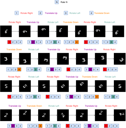
Figure 7: MNIST Transformation Task. Demonstration of NPS on the MNIST transformations task. The proposed model can be used to compose any novel combination of transformations on any digit by hand-picking the rule vector that was assigned to each corresponding operation during training.

Appendix D Coordinate Arithmetic Task

This task is mainly designed to test whether NPS can learn all the operations in the environment correctly when the operation to be performed is not provided as input and whether it can select the correct entity to apply the operation to. The task is structured as follows: We first sample a pair random coordinates $X=[(x_{i},y_{i}),(x_{j},y_{j})]$. The expected output $Y=[(\hat{x_{i}},\hat{y_{i}}),(\hat{x_{j}},\hat{y_{j}})]$ is obtained by performing a randomly selected operation on a randomly selected coordinate (hereafter referred to as "primary coordinate") from the input. Therefore, one of the coordinates from the expected output $Y$ has the same value as the corresponding coordinate in the input $X$ while the other coordinate (primary coordinate) will have a different value. Since each defined operation takes 2 arguments, we also need to select another coordinate (hereafter referred to as "contextual coordinate"), to perform the operation on the primary coordinate. This contextual coordinate is selected randomly from the input $X$. For example, if the index of the primary coordinate is $j$, the index of the contextual coordinate is $i$, and the selected transformation is Y Subtraction, then the expected output $Y=[(x_{i},y_{i}),(x_{j},y_{j}-y_{i})])$.

We use an NPS model with 4 rules. Each coordinate is a 2-dimensional vector. The slots that are input to algorithm 1 consist of a set of 4 coordinates (2 input coordinates and their corresponding output coordinates): ${\bm{X}}=[(x_{i},y_{i}),(x_{j},y_{j})]$ and $Y=[(\hat{x_{i}},\hat{y_{i}}),(\hat{x_{j}},\hat{y_{j}})]$. We concatenate the input coordinates with the corresponding output coordinates to form 4-dimensional vectors: ${\bm{X}}=[(x_{i},y_{i},\hat{x_{i}},\hat{y_{i}}),(x_{j},y_{j},\hat{x_{j}},\hat{y_{j}})]$. These make up the 2 slots that are input algorithm 1. Note that the slots are hand designed and not obtained using any convolution encoder. This is the main difference between this implementation and algorithm 1. The remaining steps of algorithm 1 are followed as is. These 2 slots are used in step 2 and step 3 of algorithm 1 to select the {primary slot, rule} pair and the contextual slot. While applying the rule MLP (i.e. step 4 of algorithm 1), we only use the input coordinates and discard the output coordinates: ${\bm{X}}=[(x_{i},y_{i}),(x_{j},y_{j})]$. We use a rule embedding dimension of 12. We use 16 as the intermediate dimension of the Rule MLP. We also use dropout with $p=0.35$ on the selection scores in subpart 3 of step 2 in algorithm 1.

For the baseline, we use similar rule MLPs as in NPS and replace the primary slot, contextual slot, rule selection procedure by a routing MLP similar to Fedus et al. [2021]. The routing MLP consists of a 4-layered MLP with intermediate dimension of 32 interleaved with Relu activations. The input to this MLP is an 8-dimension vector consisting of both the slots mentioned in the previous paragraph. The output of this MLP is passed to 3 different linear layers: one for selecting the primary slot, one for selecting the contextual slots, and one for selecting the rule. We then apply the rule MLP of the selected rules to the corresponding slots. Here again, while applying the rule MLP we discard the outputs and only use the inputs.

We evaluate the model on 2 criterion: (1) Whether it can correctly recover all available operations from the data and learn to use a separate rule to represent each operation. (2) The mean-square error between the actual output and expected output.

Setup. We generate a training dataset of 10000 examples and a test dataset of 2000 examples. We train the model for 300 epochs using a batch size of 64. We use adam optimizer for training with a learning rate of 0.0001. Training takes 15 minutes of a single GPU.

Appendix E Parallel vs Sequential Rule Application

E.1 Shapes Stack

Effect of Number of Rules. We also study the effect of number of rules on both PNPS and SNPS in the test and transfer settings. Figure 8 shows the results of our analysis. We can see that there is an optimal number of rules ${\bm{N}}={\bm{k}}$ for both PNPS and SNPS and the performance drops for ${\bm{N}}<{\bm{k}}$ and ${\bm{N}}>{\bm{k}}$. We can see that ${\bm{k}}=2$ for PNPS and ${\bm{k}}=4$ for SNPS. The drop in performance for ${\bm{N}}<{\bm{k}}$ can be attributed to lack of capacity (i.e. number of rules being less than the required number of rules for the environment). Consequently, the drop in performance for ${\bm{N}}>{\bm{k}}$ can be attributed to the availability of more than the required number of rules. The extra rules may serve as noise during the training process.

Training Details. We train the model for 1000000 iterations using a batch size of 20. The training takes 24 hours for PNPS and 48 hours for SNPS. We use a single v100 gpu for each run. We set the rule embedding dimension to 64.

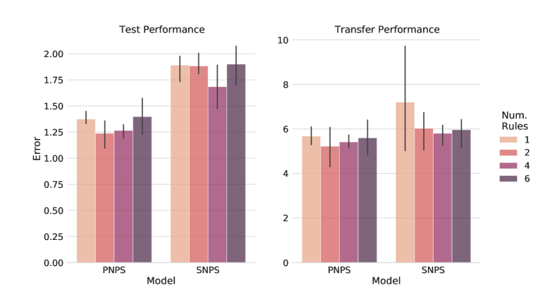
Figure 8: Here we analyse the effect of Number of Rules on both PNPS and SNPS in the shapes stack environment. We observe that there is an optimal number of rules in both cases which is 2 for PNPS and 4 for SNPS.

Model Name	Test	Transfer
OP3	0.32$\pm$0.04	0.14$\pm$0.1
SNPS	0.51$\pm$0.07	0.34$\pm$0.08

Table 9: This table shows the comparison of the proposed SNPS models against the OP3 baseline in terms of ARI scores (higher is better) on the bouncing balls task. SNPS replaces the GNN used in OP3 by rules.

E.2 Bouncing Balls

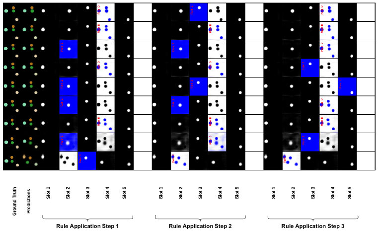
Figure 9: In the figure, we use an NPS model with 3 rules and 3 rule application steps. We analyze the entity and rule selection by NPS per time step. A rule application on a slot is shown by highlighting that slot with blue color. The index of the applied rule is also mentioned in the slot. We can see that whenever a rule is applied on the slot representing the background, rule 0 is used. On the other hand, whenever it is applied on the slots representing one of the balls, rule 1 or rule 2 are used. We can also see that rules are mainly only being applied to the two balls in the middle that are touching or close to touching while no rules are being applied to the ball on the top since it stays constant throughout this episode. The ball at the bottom is also mostly constant and receives only 1 rule application when its close to colliding with the wall.

Setup. We consider a bouncing-balls environment in which multiple balls move with billiard-ball dynamics. We validate our model on a colored version of this dataset. This task is setup as a next step prediction task where the model is supposed to predict the motion of a set of balls that follow billiard ball dynamics. The output of each of our models consists of a seperate binary mask for each object in a frame along with an rgb image corresponding to each mask which contains the rgb values for the pixels specified by that mask. During training each of the balls can have one of the four possible colors, and during testing we increase the number of balls from 4 to 6-8.

We use the following baselines for this task:

• SCOFF Goyal et al. [2020]: This factorizes knowledge in terms of object files that represent entities and schemas that represent dynamical knowledge. The object files compete to represent the input using a top-down input attention mechanism. Then, each object file updates its state using a particular schema which it selects using an attention mechanism.

• SCOFF++: Here we use SCOFF with 1 schema. We replace the input attention mechanism in SCOFF with an iterative attention mechanism as proposed in slot attention Locatello et al. [2020b]. We note that slot attention proposes to use iterative attention by building on the idea of top-down attention as proposed in [Goyal et al., 2019]. We note that slot attention was only evaluated on the static images. Here, the query is a function of the hidden state of the different object files in SCOFF from the previous timestep, which allows temporal consistency in slots across the video sequence.

For our instantiation of NPS, we replace pairwise communication attention in SCOFF++ with PNPS or SNPS. From the discussion in Section 4.2 we find that SNPS outperforms the SCOFF-based model and PNPS.

We further test the proposed SNPS model against another strong object-centric baseline called OP3 (Veerapaneni et al. [2019]). We follow the exact same setup as Weis et al. [2020]. For the proposed model we replace the GNN in OP3 with SNPS. We present the results of this comparison in Table 9. We can see that SNPS comfortably outperforms OP3.

An intuitive visualization of the rule and entity selection for the bouncing balls environment is presented in Figure 9.

Training Details. We run each model for 20 epochs with batch size 8 which amounts to 24 hours on a single v100 gpu. For the OP3 experiment, we use 5 rules and 3 rule application steps. We use a rule embedding dimension of 32 for our experiments.

E.3 Discussion of parallel vs sequential NPS

We have introduced two forms of NPS - Parallel and Sequential. Parallel NPS offers lower application sparsity as compared Sequential NPS while both have the same contextual sparsity. The same contextual sparsity indicates that the interactions or rules learned by both SNPS and PNPS are of same capacity since the rules in both take 2 arguments (primary slot and contextual slot). SNPS has the favourable property of being able to compose multiple rules by virtue of multiple rule application steps. We find that PNPS works better in environments where the nature of interactions are inherently dense and frequent which is expected due to the lower application sparsity of PNPS while SNPS works better in environments where interactions are much more rare. One caveat of this approach is that we need to know the structure of the environment beforehand to make an informed decision on whether to use SNPS or PNPS. Ideally, we would want an algorithm that can learn to use PNPS or SNPS depending on the environment. We leave this exploration for future work.

Appendix F Benefits of Sparse Interactions Offered by NPS

F.1 Sprites-MOT: Learning Rules for Physical Reasoning

Setup. We use the OP3 model Veerapaneni et al. [2019] as our baseline for this task. We follow the exact same setup as Weis et al. [2020]. To test the proposed model, we replace the GNN-based transition model in OP3 with the proposed NPS. The output of the model consists of a seperate binary mask for each object in a frame along with an rgb image corresponding to each mask which contains the rgb values for the pixels specified by the mask.

Evaluation protocol. We use the same evaluation protocol as followed by Weis et al. [2020] which is based on the MOT (Multi-object tracking) challenge Milan et al. [2016]. To compute these metrics, we have to match the objects in the predicted masks with the objects in the ground truth mask. We consider a match if the intersection over union (IoU) between the predicted object mask and ground truth object mask is greater than 0.5. The results on these metrics can be found in Table 10. We consider the following metrics:

• Matches (Higher is better): This indicates the fraction of predicted object masks that are mapped to the ground truth object masks (i.e. IoU > 0.5).

• Misses (Lower is better): This indicates the fraction of ground truth object masks that are not mapped to any predicted object masks.

• False Positives (Lower is better): This indicates the fraction of predicted object masks that are not mapped to any ground truth masks.

• Id Switches (Lower is better): This metric is designed to penalize switches. When a predicted mask starts modelling a different object than the one it was previously modelling, it is termed a an id switch. This metric indicates the fraction of objects that undergo and id switch.

• Mostly Tracked (Higher is better): This is the ratio of ground truth objects that have not undergone and id switch and have been tracked for at least 80% of their lifespan.

• Mostly Detected (Higher is Better): This the ratio of ground truth objects that have been correctly tracked for at least 80% of their lifespan without penalizing id switches.

• MOT Accuracy (MOTA) (Higher is better): This measures the fraction of all failure cases i.e. false positives, misses, and id switches as compared to the number of objects present in all frames. Concretely, MOTA is indicated by the following formula:

  $$MOTA=1-\frac{\sum_{t=1}^{T}M_{t}+FP_{t}+IDS_{t}}{\sum_{t=1}^{T}O_{t}}$$ (1)

  where, $M_{t}$, $FP_{t}$, and $IDS_{t}$ indicates the misses, false positives, id switches at timestep $t$ and $O_{t}$ indicates the number of objects at timestep $t$.

• MOT Precision (MOTP) (Higher is better): This metric measures the accuracy between the predicted object mask and the ground truth object mask relative to the total number of matches. Here, accuracy is measured in IoU between the predicted masks and ground truth mask. Concretely, MOTP is indicated using the following formula:

  $$MOTP=\frac{\sum_{t=1}^{T}\sum_{i=1}^{I}d_{t}^{i}}{\sum_{t=1}^{T}c_{t}}$$ (2)

  where, $d_{t}^{i}$ measures the accuracy for the $i^{th}$ matched object between the predicted and the ground truth mask measured in IoU. $c_{t}$ indicates the number of matches in timestep $t$.

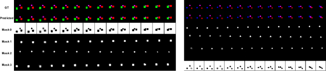
Figure 10: This figure shows the predictions of the OP3 model using the proposed NPS as a transition model. We can see that the proposed model succeeds in segregating each entity into separate slots and predicting the motion of each individual entity.

Model	MOTA $\uparrow$	MOTP $\uparrow$	Mostly Detected $\uparrow$	Mostly Tracked $\uparrow$	Match $\uparrow$	Miss $\downarrow$	ID Switches $\downarrow$	False Positives $\downarrow$
OP3	89.1$\pm$5.1	78.4$\pm$2.4	92.4$\pm$4.0	91.8$\pm$3.8	95.9$\pm$2.2	3.7$\pm$2.2	0.4$\pm$0.0	6.8$\pm$2.9
NPS	90.72$\pm$5.15	79.91$\pm$0.1	94.66$\pm$0.29	93.18$\pm$0.84	96.93$\pm$0.16	2.48$\pm$0.07	0.58$\pm$0.02	6.2$\pm$3.5

Table 10: Sprites-MOT. Comparison between the proposed NPS and the baseline OP3 for various MOT (multi-object tracking) metrics on the sprites-MOT dataset ($\uparrow$: higher is better, $\downarrow$: lower is better). Average over 3 random seeds.

Model output. We show the predictions of the proposed model in figure 10. We use 10 rules and 3 rule application steps for our experiments. We use a rule embedding dimension of 64 for our experiments. Each rule is parameterized by a neural network as described in Tab. 7.

F.2 Physics Environment

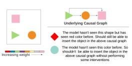
Figure 11: Demonstration of the physics environment.

A demonstration of this environment can be found in Figure 11. Each color in the environment is associated with a unique weight. The model does not have access to this information. For the model to accurately predict the outcome of an action, it needs to infer the weights from demonstrations. Inferring the correct weights will allow the model to construct the correct causal graph for each example as shown in Figure 11 which will allow it predict the correct outcome of each action in the environment. We can see that as long as the model has the correct mapping from the colors to the weights, it will be able to deal with an object of any shape irrespective of whether it has seen the shape before or not as long as it has observed the color before. Therefore, to perform well in this environment the model must infer the correct mapping from colors to weights . Learning any form of spurious correlation between the shape and the weight will penalize its performance.

The agent performs stochastic interventions (actions) in the environment to infer the weights of the blocks. Each intervention makes a block move in any of the 4 available directions (left, right, up, and down). When an intervened block $A$ with weight $W_{A}$ comes into contact with another block $B$ with weight $W_{B}$, the block $B$ may get pushed if $W_{B}<W_{A}$ else $B$ will remain still. Hence, any interaction in this environment involves only 2 blocks (i.e., 2 entities) and the other blocks are not affected. Therefore, modelling the interactions between all blocks for every intervention, as is generally done using GNNs, may be wasteful. NPS is particularly well suited for this task as any rule application takes into account only a subset of entities, hence considering interactions between those blocks only. Note that the interactions in this environment are not symmetrical and NPS can handle such relations. For example, consider a set of 3 blocks: $\{A_{0},A_{1},A_{2}\}$. If an intervention leads to $A_{1}$ pushing $A_{0}$, then NPS would apply the rule to the slot representing entity $A_{0}$. Since the movement of $A_{0}$ would depend on whether $A_{0}$ is heavier or lighter than $A_{1}$, NPS would also select the slot representing entity $A_{1}$ as a contextual slot and take it into account while applying the rule to $A_{0}$. Therefore, NPS can represent sparse and directed rules, which as we show, is more useful in this environment then learning dense and undirected relationships (or commutative operations).

Data collection. For the data, the agent performs random interventions or actions in the environment and collects the corresponding episodes. We collect 1000 episodes of length 100 for training and 10000 episodes of length 10 for evaluation.

Metrics. For this task, we evaluate the predictions of the models in the latent space. We use the following metrics described in [Kipf et al., 2019] for evaluation: Hits at Rank 1 (H@1): This score is 1 for a particular example if the predicted state representation is nearest to the encoded true observation and 0 otherwise. Thus, it measures whether the rank of the predicted representation is equal to 1 or not, where ranking is done over all reference state representations by distance to the true state representation. We report the average of this score over the test set. Note that, higher H@1 indicates better model performance. Mean Reciprocal Rank (MRR): This is defined as the average inverse rank, i.e, MRR $=\frac{1}{N}\sum_{n=1}^{N}\frac{1}{\text{rank}_{n}}$ where $\text{rank}_{n}$ is the rank of the $n^{th}$ sample of the test set where ranking is done over all reference state representations. Here also, higher MRR indicates better performance.

Setup. Here, we follow the experimental setup in Ke et al. [2021]. We use images of size $50\times 50$. We first encode the current frame ${\bm{x}}^{t}$ using a convolutional encoder and pass this encoded representation using top-down attention as proposed in [Goyal et al., 2019, 2020] to extract the separate entities in the frame as slots. We use a 4-layered convolutional encoder which preserves the spatial dimensions of the image and encodes each pixel into 64 channels. We pass this encoded representation to the object encoder which extracts the entities in the frame as $M$ 64-sized slots (${\bm{V}}_{1\ldots M}^{t}$). We then concatenate each slot with the action (${\bm{a}}^{t}$) taken in the current frame and pass this representation to NPS which selects a rule to apply to one of the slots using algorithm 1. The following equations describe our model in detail. We use $M=5$ since there are 5 objects in each frame. We use a rule embedding dimension of 64 for our experiments.

$\bullet~{}~{}$ $\hat{{\bm{x}}^{t}}=\text{Encoder}({\bm{x}}^{t})$

$\bullet~{}~{}$ ${\bm{V}}_{1...M}^{t}=\text{Slot Attention}(\hat{{\bm{x}}}^{t})$

$\bullet~{}~{}$ ${\bm{V}}_{i}^{t}=\text{Concatenate}({\bm{V}}_{i}^{t},{\bm{a}}^{t})$ $\forall\text{i}\in\{1,\ldots,M\}$

$\bullet~{}~{}$ ${\bm{V}}_{1\ldots M}^{t+1}=\text{NPS}({\bm{V}}_{1\ldots M}^{t})$

Here, NPS acts as a transition model. For the baseline, we use GNN as the transition model similar to Kipf et al. [2019].

Training Details. The objective of the model is to make accurate predictions in the latent space. Mathematically, given the current frame ${\bm{x}}^{t}$ and a set of actions ${\bm{a}}^{t},{\bm{a}}^{t+1},{\bm{a}}^{t+2},\ldots,{\bm{a}}^{k}$, the model performs these actions in the latent space as described in the above equations and predicts the latent state after applying these actions, i.e., ${\bm{V}}_{1\ldots M}^{t+k}$. Both the metrics, H@1 and MRR measure the closeness between the predicted latent state and ${\bm{V}}_{1\ldots M}^{t+k}$ and the ground truth latent state $\bar{{\bm{V}}}_{1\ldots M}^{t+k}$ which is obtained by passing frame $x^{t+k}$ through the convolutional encoder and slot attention module. During training we use the contrastive loss which optimizes the distance between the predicted and the ground truth representations. We train the model for 100 epochs (1 hour on a single v100 gpu). Mathematically, the training objective can be formulated as follows:

$$\textit{Contrastive Training }:\operatorname*{arg\,min}_{\text{Encoder, Transition}} H+\max(0,\gamma-\tilde{H})$$

$$H =\text{MSE}(\hat{{\bm{V}}}_{1\ldots M}^{t+1},{\bm{V}}_{1\ldots M}^{t+1})$$

$$\tilde{H} =\text{MSE}(\tilde{{\bm{V}}}_{1\ldots M}^{t+1},{\bm{V}}_{1\ldots M}^{t+1})$$

$$\tilde{{\bm{V}}}^{t+1} :\text{ Negative latent state obtained from random shuffling of batch}$$

$$\hat{{\bm{V}}}^{t+1} :\text{ Ground truth latent state for frame $x^{t+1}$}$$

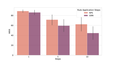
(a) Performance on MRR

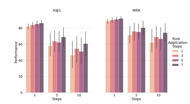
(b) Effect of Rule Application Steps on H@1 and MRR

Figure 12: Physics Environment. (a) Here we compare the performance of NPS and GNN on the MRR metric for various forward-prediction steps.(We use 1 rule and 1 rule application step) (b) Here we analyse the effect of the rule application steps on the H@1 and MRR metric for NPS. We can see that, in general, the performance increases as we increase the number of rule application steps.

Results on MRR. We show the results on the MRR metric for the physics environment in Figure 12(a). From the figure, we can see that NPS outperforms GNN on the MRR metric while predicting future steps.

Effect of Rule Application Steps. We show the effect of varying rule application steps on the physics environment in Figure 12(b). We can see that the performance increases with increasing rule application steps. Increasing the number of rule application steps seems to help since at each rule application step only sparse changes occur. We would also like to note that increasing the rule application steps comes with the cost of increased compute time due to their sequential nature.

F.3 Atari

This task is also setup as a next step prediction task in the latent space. We follow the same setup as the physics environment for this task. We use the same H@1 and MRR metric for evaluation. We test the proposed approach on 5 games: Pong, Space Invaders, Freeway, Breakout, and QBert.

Data collection. Similar to the physics environment, here also the agent performs random interventions or actions in the environment and collects the corresponding episodes. We collect 1000 episodes for training and 100 episodes for evaluation.

Performance on MRR. We present the results on the MRR metric in figure 13. We can see that NPS outperforms on GNN for steps. We use a rule embedding dimension of 32 for our experiments.

	1 Step		5 Step		10 Step
Model,	H@1	MRR	H@1	MRR	H@1	MRR
NPS	44.09 +/- 8.30	60.577 +/- 7.919	22.25 +/- 7.567	38.731 +/- 9.005	15.615 +/- 5.748	30.154 +/- 7.538
GNN	30.442 +/- 11.178	48.788 +/- 10.428	11.596 +/- 6.109	25.481 +/- 8.331	7.25 +/- 4.057	18.942 +/- 6.156

Table 11: Here we compare the performance of NPS and GNN on the pong environment in atari. We can see that NPS convincingly outperforms GNN. Results across 50 seeds.

	1 Step		5 Step		10 Step
Model,	H@1	MRR	H@1	MRR	H@1	MRR
NPS	61.269 +/- 11.576	74.558 +/- 9.425	32.827 +/- 9.179	52.981 +/- 9.073	21.385 +/- 7.118	39.173 +/- 8.505
GNN	68.75 +/- 8.44	79.942 +/- 5.662	21.673 +/- 6.81	39.635 +/- 7.395	14.712 +/- 4.932	31.0 +/- 6.26

Table 12: Here we compare the performance of NPS and GNN on the space invaders environment in atari. We can see that NPS outperforms GNN in the multiple step setting (5 and 10 step). Results across 50 seeds.

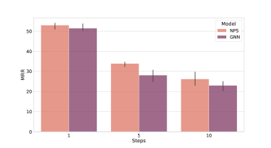
Figure 13: Atari. Here we compare the performance of NPS and GNN on the MRR metric for various forward-prediction steps. The results shown in the plot are averaged across 5 games.

References

- Ahmed et al. (2020) Ossama Ahmed, Frederik Träuble, Anirudh Goyal, Alexander Neitz, Manuel Wüthrich, Yoshua Bengio, Bernhard Schölkopf, and Stefan Bauer. Causalworld: A robotic manipulation benchmark for causal structure and transfer learning. arXiv preprint arXiv:2010.04296, 2020.
- Anderson (1987) John R Anderson. Skill acquisition: Compilation of weak-method problem situations. Psychological review, 94(2):192, 1987.
- Andreas et al. (2016) Jacob Andreas, Marcus Rohrbach, Trevor Darrell, and Dan Klein. Neural module networks. In Proceedings of the IEEE Conference on Computer Vision and Pattern Recognition, pages 39–48, 2016.
- Bahdanau et al. (2014) Dzmitry Bahdanau, Kyunghyun Cho, and Yoshua Bengio. Neural machine translation by jointly learning to align and translate. arXiv preprint arXiv:1409.0473, 2014.
- Battaglia et al. (2016) Peter W. Battaglia, Razvan Pascanu, Matthew Lai, Danilo Jimenez Rezende, and Koray Kavukcuoglu. Interaction networks for learning about objects, relations and physics. CoRR, abs/1612.00222, 2016. URL http://arxiv.org/abs/1612.00222.
- Battaglia et al. (2018) Peter W Battaglia, Jessica B Hamrick, Victor Bapst, Alvaro Sanchez-Gonzalez, Vinicius Zambaldi, Mateusz Malinowski, Andrea Tacchetti, David Raposo, Adam Santoro, Ryan Faulkner, et al. Relational inductive biases, deep learning, and graph networks. arXiv preprint arXiv:1806.01261, 2018.
- Bengio (2017) Yoshua Bengio. The consciousness prior. arXiv preprint arXiv:1709.08568, 2017.
- Bottou and Gallinari (1991) Léon Bottou and Patrick Gallinari. A framework for the cooperation of learning algorithms. In Advances in neural information processing systems, pages 781–788, 1991.
- Bronstein et al. (2017) Michael M Bronstein, Joan Bruna, Yann LeCun, Arthur Szlam, and Pierre Vandergheynst. Geometric deep learning: going beyond euclidean data. IEEE Signal Processing Magazine, 34(4):18–42, 2017.
- Bunel et al. (2018) Rudy Bunel, Matthew Hausknecht, Jacob Devlin, Rishabh Singh, and Pushmeet Kohli. Leveraging grammar and reinforcement learning for neural program synthesis. arXiv preprint arXiv:1805.04276, 2018.
- Burgess et al. (2019) Christopher P Burgess, Loic Matthey, Nicholas Watters, Rishabh Kabra, Irina Higgins, Matt Botvinick, and Alexander Lerchner. Monet: Unsupervised scene decomposition and representation. arXiv preprint arXiv:1901.11390, 2019.
- Cai et al. (2017) Jonathon Cai, Richard Shin, and Dawn Song. Making neural programming architectures generalize via recursion. arXiv preprint arXiv:1704.06611, 2017.
- Chen et al. (2018) Ricky TQ Chen, Xuechen Li, Roger Grosse, and David Duvenaud. Isolating sources of disentanglement in variational autoencoders. arXiv preprint arXiv:1802.04942, 2018.
- Ding et al. (2020) David Ding, Felix Hill, Adam Santoro, and Matt Botvinick. Object-based attention for spatio-temporal reasoning: Outperforming neuro-symbolic models with flexible distributed architectures. arXiv preprint arXiv:2012.08508, 2020.
- Du et al. (2020) Yilun Du, Kevin Smith, Tomer Ulman, Joshua Tenenbaum, and Jiajun Wu. Unsupervised discovery of 3d physical objects from video. arXiv preprint arXiv:2007.12348, 2020.
- Engelcke et al. (2019) Martin Engelcke, Adam R Kosiorek, Oiwi Parker Jones, and Ingmar Posner. Genesis: Generative scene inference and sampling with object-centric latent representations. arXiv preprint arXiv:1907.13052, 2019.
- Eslami et al. (2016) SM Eslami, Nicolas Heess, Theophane Weber, Yuval Tassa, David Szepesvari, Koray Kavukcuoglu, and Geoffrey E Hinton. Attend, infer, repeat: Fast scene understanding with generative models. arXiv preprint arXiv:1603.08575, 2016.
- Evans et al. (2019) Richard Evans, José Hernández-Orallo, Johannes Welbl, Pushmeet Kohli, and Marek Sergot. Making sense of sensory input. Artificial Intelligence, page 103438, 2019.
- Fedus et al. (2021) William Fedus, Barret Zoph, and Noam Shazeer. Switch transformers: Scaling to trillion parameter models with simple and efficient sparsity. CoRR, abs/2101.03961, 2021. URL https://arxiv.org/abs/2101.03961.
- Fernando et al. (2017) Chrisantha Fernando, Dylan Banarse, Charles Blundell, Yori Zwols, David Ha, Andrei A Rusu, Alexander Pritzel, and Daan Wierstra. Pathnet: Evolution channels gradient descent in super neural networks. arXiv preprint arXiv:1701.08734, 2017.
- Girshick (2015) Ross B. Girshick. Fast R-CNN. CoRR, abs/1504.08083, 2015. URL http://arxiv.org/abs/1504.08083.
- Goyal and Bengio (2020) Anirudh Goyal and Yoshua Bengio. Inductive biases for deep learning of higher-level cognition. arXiv preprint arXiv:2011.15091, 2020.
- Goyal et al. (2019) Anirudh Goyal, Alex Lamb, Jordan Hoffmann, Shagun Sodhani, Sergey Levine, Yoshua Bengio, and Bernhard Schölkopf. Recurrent independent mechanisms, 2019.
- Goyal et al. (2020) Anirudh Goyal, Alex Lamb, Phanideep Gampa, Philippe Beaudoin, Sergey Levine, Charles Blundell, Yoshua Bengio, and Michael Mozer. Object files and schemata: Factorizing declarative and procedural knowledge in dynamical systems. arXiv preprint arXiv:2006.16225, 2020.
- Graves et al. (2014) Alex Graves, Greg Wayne, and Ivo Danihelka. Neural turing machines. arXiv preprint arXiv:1410.5401, 2014.
- Greff et al. (2016) Klaus Greff, Antti Rasmus, Mathias Berglund, Tele Hotloo Hao, Jürgen Schmidhuber, and Harri Valpola. Tagger: Deep unsupervised perceptual grouping. arXiv preprint arXiv:1606.06724, 2016.
- Greff et al. (2019) Klaus Greff, Raphaël Lopez Kaufman, Rishabh Kabra, Nick Watters, Chris Burgess, Daniel Zoran, Loic Matthey, Matthew Botvinick, and Alexander Lerchner. Multi-object representation learning with iterative variational inference. arXiv preprint arXiv:1903.00450, 2019.
- Groth et al. (2018) Oliver Groth, Fabian Fuchs, Ingmar Posner, and Andrea Vedaldi. Shapestacks: Learning vision-based physical intuition for generalised object stacking. CoRR, abs/1804.08018, 2018. URL http://arxiv.org/abs/1804.08018.
- He et al. (2018) Zhen He, Jian Li, Daxue Liu, Hangen He, and David Barber. Tracking by animation: Unsupervised learning of multi-object attentive trackers. CoRR, abs/1809.03137, 2018. URL http://arxiv.org/abs/1809.03137.
- Higgins et al. (2016) Irina Higgins, Loic Matthey, Arka Pal, Christopher Burgess, Xavier Glorot, Matthew Botvinick, Shakir Mohamed, and Alexander Lerchner. beta-vae: Learning basic visual concepts with a constrained variational framework. 2016.
- Jacobs et al. (1991) Robert A Jacobs, Michael I Jordan, Steven J Nowlan, Geoffrey E Hinton, et al. Adaptive mixtures of local experts. Neural computation, 3(1):79–87, 1991.
- Jang et al. (2016) Eric Jang, Shixiang Gu, and Ben Poole. Categorical reparameterization with gumbel-softmax. arXiv preprint arXiv:1611.01144, 2016.
- Ke et al. (2021) Nan Rosemary Ke, Aniket Didolkar, Sarthak Mittal, Anirudh Goyal, Guillaume Lajoie, Stefan Bauer, Danilo Rezende, Yoshua Bengio, Michael Mozer, and Christopher Pal. Systematic evaluation of causal discovery in visual model based reinforcement learning. arXiv preprint arXiv:2107.00848, 2021.
- Kipf et al. (2018) Thomas Kipf, Ethan Fetaya, Kuan-Chieh Wang, Max Welling, and Richard Zemel. Neural relational inference for interacting systems. arXiv preprint arXiv:1802.04687, 2018.
- Kipf et al. (2019) Thomas Kipf, Elise van der Pol, and Max Welling. Contrastive learning of structured world models. arXiv preprint arXiv:1911.12247, 2019.
- Kirsch et al. (2018) Louis Kirsch, Julius Kunze, and David Barber. Modular networks: Learning to decompose neural computation. In Advances in Neural Information Processing Systems, pages 2408–2418, 2018.
- Kosiorek et al. (2018) Adam Kosiorek, Hyunjik Kim, Yee Whye Teh, and Ingmar Posner. Sequential attend, infer, repeat: Generative modelling of moving objects. Advances in Neural Information Processing Systems, 31:8606–8616, 2018.
- Laird et al. (1986) John E Laird, Paul S Rosenbloom, and Allen Newell. Chunking in soar: The anatomy of a general learning mechanism. Machine learning, 1(1):11–46, 1986.
- Lamb et al. (2020) Alex Lamb, Anirudh Goyal, Agnieszka Słowik, Michael Mozer, Philippe Beaudoin, and Yoshua Bengio. Neural function modules with sparse arguments: A dynamic approach to integrating information across layers. arXiv preprint arXiv:2010.08012, 2020.
- Le Roux et al. (2011) Nicolas Le Roux, Nicolas Heess, Jamie Shotton, and John Winn. Learning a generative model of images by factoring appearance and shape. Neural Computation, 23(3):593–650, 2011.
- Li et al. (2020) Yujia Li, Felix Gimeno, Pushmeet Kohli, and Oriol Vinyals. Strong generalization and efficiency in neural programs. arXiv preprint arXiv:2007.03629, 2020.
- Locatello et al. (2020a) Francesco Locatello, Dirk Weissenborn, Thomas Unterthiner, Aravindh Mahendran, Georg Heigold, Jakob Uszkoreit, Alexey Dosovitskiy, and Thomas Kipf. Object-centric learning with slot attention. arXiv preprint arXiv:2006.15055, 2020a.
- Locatello et al. (2020b) Francesco Locatello, Dirk Weissenborn, Thomas Unterthiner, Aravindh Mahendran, Georg Heigold, Jakob Uszkoreit, Alexey Dosovitskiy, and Thomas Kipf. Object-centric learning with slot attention, 2020b.
- Lovett and Anderson (2005) Marsha C Lovett and John R Anderson. Thinking as a production system. The Cambridge handbook of thinking and reasoning, pages 401–429, 2005.
- Marcus (2003) Gary F Marcus. The algebraic mind: Integrating connectionism and cognitive science. MIT press, 2003.
- McMillan et al. (1991) Clayton McMillan, Michael C Mozer, and Paul Smolensky. The connectionist scientist game: rule extraction and refinement in a neural network. In Proceedings of the 13th Annual Conference of the Cognitive Science Society, pages 424–430, 1991.
- Milan et al. (2016) Anton Milan, Laura Leal-Taixé, Ian D. Reid, Stefan Roth, and Konrad Schindler. MOT16: A benchmark for multi-object tracking. CoRR, abs/1603.00831, 2016. URL http://arxiv.org/abs/1603.00831.
- Neelakantan et al. (2015) Arvind Neelakantan, Quoc V Le, and Ilya Sutskever. Neural programmer: Inducing latent programs with gradient descent. arXiv preprint arXiv:1511.04834, 2015.
- Qi et al. (2021) Haozhi Qi, Xiaolong Wang, Deepak Pathak, Yi Ma, and Jitendra Malik. Learning long-term visual dynamics with region proposal interaction networks. In International Conference on Learning Representations, 2021. URL https://openreview.net/forum?id=_X_4Akcd8Re.
- Rahaman et al. (2020) Nasim Rahaman, Anirudh Goyal, Muhammad Waleed Gondal, Manuel Wuthrich, Stefan Bauer, Yash Sharma, Yoshua Bengio, and Bernhard Schölkopf. S2rms: Spatially structured recurrent modules. arXiv preprint arXiv:2007.06533, 2020.
- Rand (1971) William M Rand. Objective criteria for the evaluation of clustering methods. Journal of the American Statistical association, 66(336):846–850, 1971.
- Raposo et al. (2017) David Raposo, Adam Santoro, David Barrett, Razvan Pascanu, Timothy Lillicrap, and Peter Battaglia. Discovering objects and their relations from entangled scene representations. arXiv preprint arXiv:1702.05068, 2017.
- Reed and De Freitas (2015) Scott Reed and Nando De Freitas. Neural programmer-interpreters. arXiv preprint arXiv:1511.06279, 2015.
- Ronco et al. (1997) Eric Ronco, Henrik Gollee, and Peter J Gawthrop. Modular neural networks and self-decomposition. Technical Report CSC-96012, 1997.
- Rosenbaum et al. (2017) Clemens Rosenbaum, Tim Klinger, and Matthew Riemer. Routing networks: Adaptive selection of non-linear functions for multi-task learning. arXiv preprint arXiv:1711.01239, 2017.
- Rosenbaum et al. (2019) Clemens Rosenbaum, Ignacio Cases, Matthew Riemer, and Tim Klinger. Routing networks and the challenges of modular and compositional computation. arXiv preprint arXiv:1904.12774, 2019.
- Scarselli et al. (2008) Franco Scarselli, Marco Gori, Ah Chung Tsoi, Markus Hagenbuchner, and Gabriele Monfardini. The graph neural network model. IEEE Transactions on Neural Networks, 20(1):61–80, 2008.
- Schrittwieser et al. (2020) Julian Schrittwieser, Ioannis Antonoglou, Thomas Hubert, Karen Simonyan, Laurent Sifre, Simon Schmitt, Arthur Guez, Edward Lockhart, Demis Hassabis, Thore Graepel, et al. Mastering atari, go, chess and shogi by planning with a learned model. Nature, 588(7839):604–609, 2020.
- Shazeer et al. (2017) Noam Shazeer, Azalia Mirhoseini, Krzysztof Maziarz, Andy Davis, Quoc Le, Geoffrey Hinton, and Jeff Dean. Outrageously large neural networks: The sparsely-gated mixture-of-experts layer. arXiv preprint arXiv:1701.06538, 2017.
- Tacchetti et al. (2018) Andrea Tacchetti, H Francis Song, Pedro AM Mediano, Vinicius Zambaldi, Neil C Rabinowitz, Thore Graepel, Matthew Botvinick, and Peter W Battaglia. Relational forward models for multi-agent learning. arXiv preprint arXiv:1809.11044, 2018.
- Touretzky and Hinton (1988) David S Touretzky and Geoffrey E Hinton. A distributed connectionist production system. Cognitive science, 12(3):423–466, 1988.
- Trask et al. (2018) Andrew Trask, Felix Hill, Scott E Reed, Jack Rae, Chris Dyer, and Phil Blunsom. Neural arithmetic logic units. In Advances in Neural Information Processing Systems, pages 8035–8044, 2018.
- Van Steenkiste et al. (2018) Sjoerd Van Steenkiste, Michael Chang, Klaus Greff, and Jürgen Schmidhuber. Relational neural expectation maximization: Unsupervised discovery of objects and their interactions. arXiv preprint arXiv:1802.10353, 2018.
- Vaswani et al. (2017) Ashish Vaswani, Noam Shazeer, Niki Parmar, Jakob Uszkoreit, Llion Jones, Aidan N. Gomez, Lukasz Kaiser, and Illia Polosukhin. Attention is all you need, 2017.
- Veerapaneni et al. (2019) Rishi Veerapaneni, John D. Co-Reyes, Michael Chang, Michael Janner, Chelsea Finn, Jiajun Wu, Joshua B. Tenenbaum, and Sergey Levine. Entity abstraction in visual model-based reinforcement learning. CoRR, abs/1910.12827, 2019. URL http://arxiv.org/abs/1910.12827.
- Veerapaneni et al. (2020) Rishi Veerapaneni, John D Co-Reyes, Michael Chang, Michael Janner, Chelsea Finn, Jiajun Wu, Joshua Tenenbaum, and Sergey Levine. Entity abstraction in visual model-based reinforcement learning. In Conference on Robot Learning, pages 1439–1456. PMLR, 2020.
- Watters et al. (2017) Nicholas Watters, Daniel Zoran, Theophane Weber, Peter Battaglia, Razvan Pascanu, and Andrea Tacchetti. Visual interaction networks: Learning a physics simulator from video. In Advances in neural information processing systems, pages 4539–4547, 2017.
- Weis et al. (2020) Marissa A. Weis, Kashyap Chitta, Yash Sharma, Wieland Brendel, Matthias Bethge, Andreas Geiger, and Alexander S. Ecker. Unmasking the inductive biases of unsupervised object representations for video sequences, 2020.
- Xu et al. (2018) Danfei Xu, Suraj Nair, Yuke Zhu, Julian Gao, Animesh Garg, Li Fei-Fei, and Silvio Savarese. Neural task programming: Learning to generalize across hierarchical tasks. In 2018 IEEE International Conference on Robotics and Automation (ICRA), pages 1–8. IEEE, 2018.
- Zablotskaia et al. (2020) Polina Zablotskaia, Edoardo A Dominici, Leonid Sigal, and Andreas M Lehrmann. Unsupervised video decomposition using spatio-temporal iterative inference. arXiv preprint arXiv:2006.14727, 2020.