Backward energy flow in simple 4-wave electromagnetic fields

Abstract

Electromagnetic energy backflow is a phenomenon occurring in regions where the direction of the Poynting vector is opposite to that of the propagation of the wave field. It is particularly remarkable in the nonparaxial regime and has been exhibited in the focal region of sharply focused beams, for vector Bessel beams, and vector-valued spatiotemporally localized waves. A detailed study is undertaken of this phenomenon and the conditions for its appearance are examined in detail in the case of a superposition of four plane waves in free space, the simplest electromagnetic arrangement for the observation of negative energy flow, as well as its comprehensive and transparent physical interpretation. It is shown that the state of polarization of the constituent components of the electromagnetic plane wave quartet determines whether energy backflow takes place or not and what values the energy flow velocity assumes. Depending on the polarization angles, the latter can assume any value from $c$ (the speed of light in vacuum) to $-c$ in certain spatiotemporal regions of the field.

• Keywords: Poynting vector, energy velocity, polarization, energy backflow

1 Introduction

Energy backflow of a free-space electromagnetic (EM) field is an unusual effect exhibited in regions where the direction of the Poynting vector is opposite to the propagation direction of the wave field. In this sense, the terms ’reversed’ or ’negative’ Poynting vector are also used. The effect is particularly remarkable in the case of non-paraxial propagation and occurs, e.g., in the focal region of sharply focused optical beams [1]-[3], in superpositions of four plane waves directed under equal angles $\theta$ with respect to the propagation axis [4, 5], for vector Bessel beams [6]-[10] and vector X-waves [11]. Note that Bessel beams are superpositions of infinitely many monochromatic plane waves making an angle $\theta$ with respect to a specific axis (say $z$) which corresponds to the direction of propagation of the Bessel beam, and X-waves—representatives of the rich family of so-called localized waves—are just the same superpositions of ultrashort pulses [12]-[15]. Energy backflow has attracted much interest in connection with applications in microparticle manipulation like ’tractor beams’, etc., see reviews [16, 17].

Our purpose is to study in detail the mechanism and conditions for the appearance of the reversed Poynting vector in a quartet of plane waves—the simplest of EM fields for observation of the effect. In distinction from earlier studies, we consider time-dependent EM fields instead of common cycle-averaged ones, and make use of the energy flow velocity. Although the latter is given by a well-known formula related to the Poynting vector and the energy density, it exhibits some surprising properties. We hope that such a study will result in a more comprehensible and transparent picture of the nature of the backward energy flow effect than it can be deduced from cumbersome formulas describing the effect in the case of the vector Bessel beams and other more complicated fields.

In the next two sections we shall study a quartet of plane waves and show how the polarizations of the constituents of the quartet determine whether the energy backflow takes place or not, and what values the energy flow velocity assumes. Section IV is devoted to studying of a general dependence of the energy flow velocity on the polarization angles. In section V we discuss the results, touch on the problem of physical interpretation of the Poynting vector and some alternative definitions—noteworthy in the given context—of the energy flow velocity. Concluding remarks are provided in section VI.

2 4-wave fields with regions of negative energy velocity

A quartet of plane waves symmetrically directed with respect to the propagation axis of the whole field constitute the simplest EM field for which energy backflow is possible. In order to study the superposition of four interfering plane waves of different polarizations, we start from a ”seed” plane wave propagating along the axis $z$ with the wavevector $\mathbf{k}_{0}=\left(0,0,k\right)$ and polarization vector $\mathbf{e}_{0}\left(\phi\right)=\left(\cos\phi,\sin\phi,0\right)$, where $\phi$ is an arbitrary angle of (linear) polarization with respect to the axis $x$. By making use of well-known rotation $\left(3\times 3\right)$-matrices $\mathbf{R}_{x}\left(\theta\right)$ and $\mathbf{R}_{y}\left(\theta\right)$ which rotate vectors by an angle $\theta$ about the $x$- and $y$-axis, respectively, we express the wave vectors of our quartet of plane waves (see figure 1) as follows:

$$\mathbf{k}_{1} =\mathbf{R}_{y}\left(\theta\right)\mathbf{k}_{0}\;,$$

$$\mathbf{k}_{2} =\mathbf{R}_{x}\left(-\theta\right)\mathbf{k}_{0}\;,$$ (1)

$$\mathbf{k}_{3} =\mathbf{R}_{y}\left(-\theta\right)\mathbf{k}_{0}\;,$$

$$\mathbf{k}_{4} =\mathbf{R}_{x}\left(\theta\right)\mathbf{k}_{0}\;.$$

In this section we study the case where the ”seed” wave for all four waves is polarized along the axis $x$, i.e., $\phi=0$. Consequently, we obtain the following polarization vectors in the quartet:

$$\mathbf{e}_{1} =\mathbf{R}_{y}\left(\theta\right)\mathbf{e}_{0}\left(0\right)=\left(\cos\theta,0,-\sin\theta\right),$$

$$\mathbf{e}_{2} =\mathbf{R}_{x}\left(-\theta\right)\mathbf{e}_{0}\left(0\right)=\left(1,0,0\right),$$ (2)

$$\mathbf{e}_{3} =\mathbf{R}_{y}\left(-\theta\right)\mathbf{e}_{0}\left(0\right)=\left(\cos\theta,0,\sin\theta\right),$$

$$\mathbf{e}_{4} =\mathbf{R}_{x}\left(\theta\right)\mathbf{e}_{0}\left(0\right)=\left(1,0,0\right),$$

which are also depicted in figure 1.

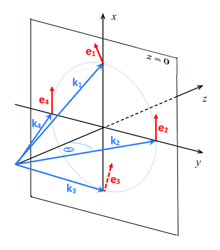
Figure 1: Wave and polarization vectors for the quartet of plane waves according to Eqs. (1) and Eq. (2).

Our aim is to study not only spatial but also temporal dependence of energy flow, i.e. we cannot restrict ourselves to calculation of a cycle-averaged Poynting vector. Therefore, instead of complex field expressions we have to work with real ones. We assume a spatio-temporal dependence of the constituent plane waves of the form $\cos\left(\mathbf{kr}-kct\right)$, where $k=\omega/c=2\pi/\lambda$ and $\mathbf{r}=\left(x,y,z\right)$. As a matter of fact, if the cosine is multiplied by a pulse envelope or replaced by any other suitable real function describing the pulse, some final results will still hold. So we get for the electric field of the quartet

$$\mathbf{E}\left(x,y,z,ct\right) ={\displaystyle\sum\limits_{j=1}^{4}}\cos\left(\mathbf{k}_{j}\mathbf{r}-kct\right)\mathbf{e}_{j}=$$ (6)

$$=\left(\begin{array}[c]{c}2\cos(kz\cos\theta-kct)\left[\cos\left(ky\sin\theta\right)+\cos\left(kx\sin\theta\right)\cos\theta\right]\\ 0\\ 2\sin(kz\cos\theta-kct)\sin\left(kx\sin\theta\right)\sin(\theta)\end{array}\right),$$

where unity amplitude of each plane wave has been assumed. Eq. (6) indicates that the field propagates along the axis $z$ due to the symmetry of the pairs of plane waves in the quartet. Likewise for the magnetic field we get

$$\mathbf{B}\left(x,y,z,ct\right) ={\displaystyle\sum\limits_{j=1}^{4}}\cos\left(\mathbf{k}_{j}\mathbf{r}-kct\right)\left(\mathbf{k}_{j}\times\mathbf{e}_{j}\right)=$$ (10)

$$=\left(\begin{array}[c]{c}0\\ 2\cos(kz\cos\theta-kct)\left[\cos\left(kx\sin\theta\right)+\cos\left(ky\sin\theta\right)\cos\theta\right]\\ 2\sin(kz\cos\theta-kct)\sin\left(ky\sin\theta\right)\sin(\theta)\end{array}\right),$$

where Heaviside–Lorentz units ($\varepsilon_{0}=\mu_{0}=1$) and normalized speed of light $c=1$ are assumed. In the given units the Poynting vector $\mathbf{S}$ and the energy density $w$ are given by

$$\mathbf{S}\left(x,y,z,ct\right) = \mathbf{E}\left(x,y,z,ct\right)\times\mathbf{B}\left(x,y,z,ct\right),$$

$$w\left(x,y,z,ct\right) = \frac{1}{2}\left[\mathbf{E}^{2}\left(x,y,z,ct\right)+\mathbf{B}^{2}\left(x,y,z,ct\right)\right].$$ (11)

For the quartet the expression of $\mathbf{S}$ turns out to be not too cumbersome if one introduces the following rescaled and dimensionless coordinates: $\widetilde{x}\equiv k~{}x\sin\theta$, $\widetilde{y}\equiv k~{}y\sin\theta$, $\widetilde{z}\equiv k~{}z\cos\theta$, $\widetilde{t}\equiv kct$. With these definitions we obtain

$$\mathbf{S}\left(\widetilde{x},\widetilde{y},\widetilde{z},\widetilde{t}\right)=\left(\begin{array}[c]{c}-4\cos\left(\widetilde{z}-\widetilde{t}\right)\sin\left(\widetilde{z}-\widetilde{t}\right)\sin\theta\sin\widetilde{x}~{}\left(\cos\widetilde{x}+\cos\widetilde{y}\cos\theta\right)\\ -4\cos\left(\widetilde{z}-\widetilde{t}\right)\sin\left(\widetilde{z}-\widetilde{t}\right)\sin\theta\sin\widetilde{y}~{}\left(\cos\widetilde{y}+\cos\widetilde{x}\cos\theta\right)\\ 4\cos^{2}\left(\widetilde{z}-\widetilde{t}\right)\left(\cos\widetilde{x}+\cos\widetilde{y}\cos\theta\right)\left(\cos\widetilde{y}+\cos\widetilde{x}\cos\theta\right)\end{array}\right).$$ (12)

From Eq. (12) the following conclusions can be drawn:

1. the field of the Poynting vector propagates as a whole with velocity $v=c/\cos\theta$ along the axis $z$ and it is invariant because it depends on time only through the difference $z\cos\theta-ct$ (we name it as the propagation variable);

2. if $z=t=0$ and generally on planes $k(z\cos\theta-ct)=n\pi,~{}n\in\mathbb{Z}$ the transverse components of $\mathbf{S}$ vanish;

3. on planes $k(z\cos\theta-ct)=(2n+1)\pi/2,~{}n\in\mathbb{Z}$ the field $\mathbf{S}$ vanishes;

4. the longitudinal component $S_{z}$ is invariant with respect to interchange of coordinates $x$ and $y$;

5. the transverse components transform to each other if the coordinates $x$ and $y$ are interchanged;

6. there are regions in any transverse plane where the longitudinal component $S_{z}$ is negative, i.e., the energy flows backward and this phenomenon takes place irrespectively of time instant or cycle averaging, although the latter affects the numerical value of negative $S_{z}$.

The energy density is given as follows in terms of the dimensionless coordinates:

$$w\left(\widetilde{x},\widetilde{y},\widetilde{z},\widetilde{t}\right) = 2\cos^{2}\left(\widetilde{z}-\widetilde{t}\right)[\left(1+\cos^{2}\theta\right)\cos^{2}\widetilde{x}+4\cos\theta\cos\widetilde{x}\cos\widetilde{y}+$$

$$\left(1+\cos^{2}\theta\right)\cos^{2}\widetilde{y}]+2\sin^{2}\left(\widetilde{z}-\widetilde{t}\right)\left(\sin^{2}\widetilde{x}+\sin^{2}\widetilde{y}\right)\sin^{2}\theta.$$

Similarly to $S_{z}$, the energy density obeys the symmetry $w\left(x,y,z,ct\right)=w\left(y,x,z,ct\right).$ This conclusion is confirmed by numerically calculated plots, an example of which is presented in figure 2.

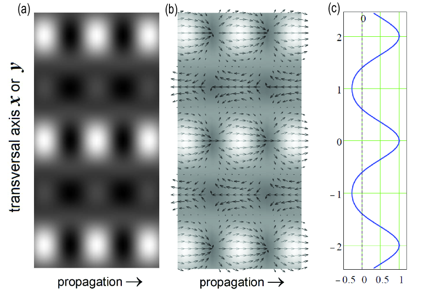
Figure 2: Energy density and energy flow for the quartet of plane EM waves with polarization vectors given by Eq. (2) and $\theta=2\pi/5=72^{\circ}$. (a)—greyscale plot of $w$ as a function of the transverse coordinate $\widetilde{x}$ at $\widetilde{y}=0$ (or $\widetilde{y}$ at $\widetilde{x}=0$) and the propagation variable $\widetilde{z}-\widetilde{t}$; (b)—the same with decreased contrast and superimposed by a vector field plot of the energy flow velocity. Shown are projections of the velocity vectors onto the plane $\left(z,x\right)$; (c)—dependence on $\widetilde{x}$ (along vertical axis) of normalized longitudinal ($z$-) component of the Poynting vector $S_{z}(\widetilde{x},0,0,0)/S_{z}(0,0,0,0)$ showing the minimal values  $-0.28$. The range of the vertical axes is $[-2.5\pi,2.5\pi]$ and of the propagation axes is $[-1.25\pi,1.25\pi]$. In plot (c) the scale of the transversal coordinate $\widetilde{x}=kx\sin\theta$ along the vertical is shown in units of $\pi$.

The interference pattern in the energy density (figure 2a) remarkably differs from that of two plane waves: if the pair (waves # 2,4) were removed from the quartet, all maxima would become of equal intensity (e.g., five equally bright maxima along the central vertical $\widetilde{z}-\widetilde{t}=0$ instead of three in figure 2a). Since the magnitude of the Poynting vector $\mathbf{S}$ is strong enough only in regions of local maxima and therefore a vector field plot of $\mathbf{S}$ would be of low distinctness, we present the vector field plot of the energy flow velocity $\mathbf{V}=\mathbf{S}/w$ instead. Figure 2b clearly reveals that at locations of weak maxima of $\ w$ the energy flows backward. While the strength of the component $S_{z}$ at these locations comprises only 28 % (see figure 2c) of that in locations of strong maxima of $w$, the velocities $\mathbf{V}$ have exactly the same absolute value 1 (or $c$ with dimensions) but the opposite signs. Numerical evaluation shows—and it is evident from figure 2b also—that wherever the velocity is purely longitudinal it equals to the physically maximal possible value $\pm c$ (small irregularities in the vector field at points of vanishing $w$ are computational artifacts due to ”zero divide by zero”). We point out the very noteworthy result that energy backflow occurs also with velocity $c$. While according to Eqs. (6) and (10) neither of the fields $\mathbf{E}$ or $\mathbf{B}$ is transverse, at locations where $V_{z}\mathbf{=}\pm c$ the fields are locally TEM, mutually perpendicular and of equal magnitude (in the chosen units)—as they have to be for a null EM field.

Note that the velocity components $V_{z}$ and $V_{x}$ on the plane $\left(y=0\right)$ constitute the vector field plot in figure 2b. If instead we plotted figure 2b with $V_{z}$ and $V_{y}$ in the same plane, we would obtain another projection of the energy flow velocity, where all arrows would be directed with respect to the axis $z$ either parallel (in the regions of stronger maxima of $w$) or antiparallel (in the regions of weaker maxima of $w$). This is understandable because according to Eq. (12) $S_{y}$ vanishes on the plane $\left(y=0\right)$.

Naturally, the smaller the angle $\theta$ the less remarkable will be the backflow effect: peak negative values of the normalized $S_{z}$ decrease to $11\%$ if $\theta=\pi/3$ and to $3\%$ if $\theta=\pi/4$. Of course, in the case of paraxial geometry the energy backflow vanishes. However, the abovementioned characteristic features of the velocity vector field remain unchanged with decreasing $\theta$, except transverse narrowing of the backflow channels.

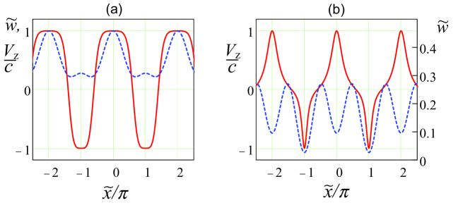
Figure 3: Dependence of the longitudinal component of the energy velocity $V_{z}$ (solid curve) and the normalized energy density (dashed curve) $\widetilde{w}\equiv w(\widetilde{x},\widetilde{y},\widetilde{z},\widetilde{t})/w(0,0,0,0)$ on the dimensionless transverse coordinate $\widetilde{x}\equiv kx\sin\theta$; (a)—along the line $y=0$ on the plane $(\widetilde{z}-\widetilde{t}=0)$ and (b)—along the line $y=0$ on the plane $(\widetilde{z}-\widetilde{t}=0.4\pi)$. Note that in the plot (b) the scale for $\widetilde{w}$  is on the right-hand side and differs from the joint scale for $V_{z}$ and $\widetilde{w}$ in (a).

Similar narrowing of the backflow channels is observable also if one moves away from the planes $\widetilde{z}-\widetilde{t}=n\pi,~{}n\in\mathbb{Z}$. Curves in figure 3 show the dependence of the longitudinal component of the energy flow velocity in comparison with that of the energy density along the central vertical in figure 2b, i.e., where $\widetilde{z}-\widetilde{t}=0$. We see in figure 3a that transverse widths of the regions where $V_{z}=\pm c$ are approximately equal to FWHM of the maxima of $w$. But on the plane $\widetilde{z}-\widetilde{t}=0.4\pi$, which is close to the plane $\widetilde{z}-\widetilde{t}=\pi/2$ where $V=0$, the backflow regions narrow substantially and their FWHM become about two times less than those of the minima or maxima of the energy density. By introducing the separate secondary scale for $\widetilde{w}\left(x,0,0.4\pi,0\right)=w\left(x,0,0.4\pi,0\right)/w\left(0,0,0,0\right)$ on the right border of the plot, it is clearly seen in figure 3b that the negative minima of $V_{z}$ are encompassed by the (positive) minima of $\widetilde{w}$.

In the discussion so far it has been assumed that the seed polarization angle $\phi=0$. However, it turns out in general that neither $\mathbf{S}$ nor $\mathbf{V}$ depend on the angle of polarization $\phi$ (if its value is the same for all four waves). This is understandable because despite the fact that the polarization vectors of the quartet do depend on $\phi$ according to Eq. (2), the combination of their mutual relative directions, which determines $\mathbf{S}$ and $w$, is invariant.

3 4-wave fields without regions of negative energy velocity

A closer study of the effect of the angle $\phi$ on the energy flow reveals that what is essential is the difference between the angle $\phi_{13}$ for the pair $(1,3)$ and the angle $\phi_{24}$ for the pair $(2,4)$ in the quartet of waves. Thus, if $\phi_{13}-\phi_{24}=0$, we return to the results of the previous section. Of special interest are the cases $\phi_{13}-\phi_{24}=\pm\pi/2$. Since the polarization vectors together with fields $\mathbf{E}$ and $\mathbf{B}$ depend on both $\phi_{13}$ and $\phi_{24}$, we prescribe values to them separately and for simplicity make one of them equal to zero. So, first we consider the case $\phi_{13}=\pi/2$ and $\phi_{24}=0$. Then $\mathbf{e}_{1}=\mathbf{e}_{3}=\left(0,1,0\right)$ and $\mathbf{e}_{2}=\mathbf{e}_{4}=\left(1,0,0\right),$ i.e., the pair $(1,3)$ is nothing but a replica of the pair $(2,4)$ rotated about the axis $z$ clockwise by $\pi/2$. Analogously to Eq. (6) and introducing the dimensionless arguments, we obtain

$$\mathbf{E}\left(\widetilde{x},\widetilde{y},\widetilde{z},\widetilde{t}\right)=\left(\begin{array}[c]{c}2\cos\left(\widetilde{z}-\widetilde{t}\right)\cos\widetilde{y}\\ 2\cos\left(\widetilde{z}-\widetilde{t}\right)\cos\widetilde{x}\\ 0\end{array}\right)$$ (13)

and likewise for the magnetic field

$$\mathbf{B}\left(\widetilde{x},\widetilde{y},\widetilde{z},\widetilde{t}\right)=\left(\begin{array}[c]{c}-2\cos\left(\widetilde{z}-\widetilde{t}\right)\cos\widetilde{x}\cos\theta\\ 2\cos\left(\widetilde{z}-\widetilde{t}\right)\cos\widetilde{y}\cos\theta\\ -2\sin\left(\widetilde{z}-\widetilde{t}\right)\left(\sin\widetilde{x}-\sin\widetilde{y}\right)\sin\theta\end{array}\right).$$ (14)

We see that in the given case the EM field as a whole is transverse electric (TE). Eq. (11) gives for the Poynting vector and the energy density the expressions

$$\mathbf{S}\left(\widetilde{x},\widetilde{y},\widetilde{z},\widetilde{t}\right)=\left(\begin{array}[c]{c}-4\cos\left(\widetilde{z}-\widetilde{t}\right)\sin\left(\widetilde{z}-\widetilde{t}\right)\sin\theta\cos\widetilde{x}~{}\left(\sin\widetilde{x}-\sin\widetilde{y}\right)\\ 4\cos\left(\widetilde{z}-\widetilde{t}\right)\sin\left(\widetilde{z}-\widetilde{t}\right)\sin\theta\cos\widetilde{y}~{}\left(\sin\widetilde{x}-\sin\widetilde{y}\right)\\ 4\cos^{2}\left(\widetilde{z}-\widetilde{t}\right)\cos\theta\left(\cos^{2}\widetilde{x}+\cos^{2}\widetilde{y}\right)\end{array}\right)$$ (15)

and

$$w\left(\widetilde{x},\widetilde{y},\widetilde{z},\widetilde{t}\right) = 2\cos^{2}\left(\widetilde{z}-\widetilde{t}\right)\left(1+\cos^{2}\theta\right)\left(\cos^{2}\widetilde{x}+\cos^{2}\widetilde{y}\right)+$$

$$2\sin^{2}\left(\widetilde{z}-\widetilde{t}\right)\sin^{2}\theta\left(\sin^{2}\widetilde{x}-\sin^{2}\widetilde{y}\right).$$

Conclusions from Eq. (15) are the same as those derived from Eq. (12) in the previous section, but with one essential exception: the 6th conclusion now is that the longitudinal component $S_{z}$ cannot take negative values, i.e., the energy flows only forward (of course, it is assumed that $|\theta|\leq\pi/2$ since otherwise the constituent plane waves would propagate backward). These conclusions, including the absence of energy backward flow are confirmed by numerically calculated plots, see figure 4.

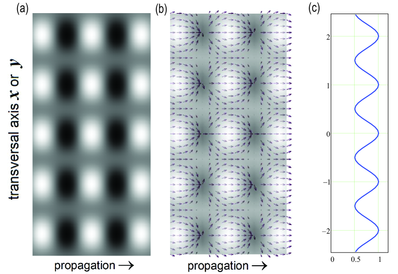
Figure 4: Energy density (a) and energy flow (b,c) of the quartet of EM plane waves with polarization vectors $\mathbf{e}_{1}=\mathbf{e}_{3}=\left(0,1,0\right)$ and $\mathbf{e}_{2}=\mathbf{e}_{4}=\left(1,0,0\right)$ in which case energy flows only in the positive direction of the axis $z$. For other parameters and scales see the caption of figure 2.

As seen in figure 4, all maxima of the energy density are of equal intensity, the energy velocity vector field is the same at all maxima and contains no backward flow. But what is very noteworthy is that everywhere the energy velocity is essentially subluminal (less than $c$) and wherever the energy flows along the propagation axis $z,$ its velocity is given by the expression

$$\frac{\left|\mathbf{V}\right|}{c}=\frac{V_{z}}{c}=\frac{2\beta}{\beta^{2}+1}=\frac{2\beta^{-1}}{\beta^{-2}+1}~{},$$ (16)

where $\beta=\cos\theta$. In figure 4, we obtain for $\theta=2\pi/5$ the value $V_{z}=0.564c$. Precisely the same value comes out from Eq. (16). For comparison, as mentioned in the previous section, all fields $\mathbf{E,B,S}$, and $w$ propagate with velocity $v=c/\cos\theta=\beta^{-1}c=3.24c,$ i.e., superluminally. Eq. (16) was first found in [18] where it was shown that various fields—crossing plane waves, Bessel beams, Bessel-X pulses and other propagation-invariant wave fields obey this relation between the axial phase- or group velocity and energy flow velocity.

Next, we consider the case $\phi_{13}=0$ and $\phi_{24}=\pi/2$. Then the polarization vectors in the quartet turn out to be

$$\mathbf{e}_{1} =\left(\cos\theta,0,-\sin\theta\right),$$

$$\mathbf{e}_{2} =\left(0,\cos\theta,-\sin\theta\right),$$

$$\mathbf{e}_{3} =\left(\cos\theta,0,\sin\theta\right),$$ (17)

$$\mathbf{e}_{4} =\left(0,\cos\theta,\sin\theta\right),$$

i.e., the pair $(2,4)$ is nothing but a replica of the pair $(1,3)$ rotated about the axis $z$ clockwise by $\pi/2$. In contradistinction to the previous case, the EM field now is transverse magnetic (TM) and the magnetic field turns out to be equal to Eq. (13) but with minus sign in front of the first component. The expression for the Poynting vector turns out to be the same as in Eq. (15) if in the latter the difference of sines is replaced by their sum and the factor $4$ in the second component by $-4$. As a result, the quartet with polarization vectors of Eq. (17) exhibits the same subluminal velocity of the energy flow as in the previous case and figure 4 illustrates equally well the present case. In [18] we have shown that (i) a TM field of a symmetrical pair of plane waves—the propagating direction of the first one lies on the $(x,z)$ plane and is inclined by angle $+\theta$ with respect to the $z$-axis, and the second one by angle $-\theta$ on the same plane—exhibit subluminal energy velocity along the axis $z$ according to Eq. (16); (ii) any superpositions of such pairs rotated about the axis $z$ have the same property.. The quartet of the present case is just a particular example of such superposition where the two pairs are rotated clockwise by $\pi/2$.

To conclude, from the results of sections 2 and 3 a general rule follows: if the EM field of the wave quartet is purely TE or TM, there is no backward energy flow and its (forward) velocity is subluminal obeying Eq. (12); otherwise not only forward but also backward energy flow takes place, both with luminal velocity $c$.

4 Dependence of energy velocity on polarization angles: general case

Since the energy flow velocity field so drastically depends on whether $\phi_{13}=\pi/2$ or $\phi_{13}=0$, it is of interest to study the dependence over the full range of angle $\phi_{13}=\phi\in[0,\pi]$ (keeping $\phi_{24}\ =0)$. Let us focus, in particular, on regions where $\mathbf{V}$ is parallel or antiparallel to the axis $z$ and has magnitude $\left|\mathbf{V}\right|/c=1$ or $V_{z}/c=\pm 1$, see figure 2. For the sake of definiteness we consider two points on the axis $x$: first, the point where $\widetilde{x}=\widetilde{y}=\widetilde{z}-\widetilde{t}=0$ and, second, where $\widetilde{x}=\pi$, $\widetilde{y}=\widetilde{z}-\widetilde{t}=0$. For the first point we obtain

$$\frac{V_{z}}{c}=\frac{2\cos\theta+\cos\phi+\cos\phi\cos^{2}\theta}{\cos^{2}\theta+1+2\cos\phi\cos\theta},$$ (18)

which for $\phi=0$ reduces to $V_{z}/c=1$ as it has to, see figure 2 and for $\phi=\pi/2$ reduces to Eq. (16) as it also has to, see figure 4. For the second point a slightly modified version of Eq. (18) comes out: only a replacement $\cos\phi\rightarrow-\cos\phi$ must be done. Again, the modified expression for $\phi=0$ reduces to $V_{z}/c=-1$ and for $\phi=\pi/2$ to Eq. (16), as expected. The behaviour of $V_{z}/c$ over the full range of angle is depicted in figure 5.

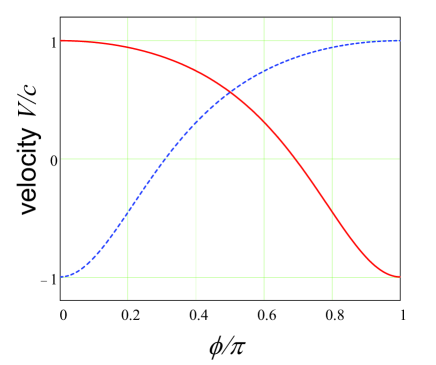
Figure 5: Dependence of the energy flow velocity on the angle $\phi$ for points $\widetilde{x}=0$ (solid curve) and $\widetilde{x}=\pi$ (dashed curve) according to Eq. (18).

We see that if $\phi=\pi/2$ the velocity is given by Eq. (16) in accord with figure 4. At values $\phi$ close to $\pi$ the regions of forward and backward flow of energy interchange. Equating the nominator of Eq. (18) to zero allows one to answer the question: what are the values of $\phi$ at which the energy backflow disappears, i.e., both curves in figure 5 become positive? The answer is: $\phi$ must obey the condition $\cos\phi=\pm 2\cos\theta/\left(\cos^{2}\theta+1\right)$, i.e., the right-hand-side of Eq. (16). Whether such a surprising coincidence has a deeper physical meaning, needs further study.

Similarly to the preceding section we also studied the behaviour of the velocity if the values of angles $\phi_{13}$ and $\phi_{24}$ are interchanged, i.e. the velocity dependence on $\phi_{24}$ over the full range of angle $\phi_{24}=\phi\in[0,\pi]$ (keeping $\phi_{13}\ =0)$. Although the interchange of the angles alters the fields $\mathbf{E}$ and $\mathbf{B}$ (interchange their components and signs), the Poynting vector $\mathbf{S}$, as well as the energy density $w$ and therefore also $\mathbf{V}$ remain unchanged. Hence, the results given above hold in this case as well.

5 Discussion

Since the variable along the horizontal axis in figures 2a, 2b, 4a, and 4b is $z\cos\theta-ct$, these plots can be viewed either as $z$-dependence or time dependence of the fields. The latter viewpoint allows one to read out from these plots what would be the temporally cycle-averaged quantities commonly evaluated from complex-valued EM fields. We see that the direction of energy flow does not flip in time (and/or along the axis $z$) and, in particular, where it flows backward in figure 2b, it does so all time. Also, the transverse components of the velocity vanish as a result of such averaging. This follows already from symmetry considerations and from the observation that the product $\cos\left(\widetilde{z}-\widetilde{t}\right)\sin\left(\widetilde{z}-\widetilde{t}\right)$ entering the transverse components in Eqs. (12) and (15) vanishes after cycle averaging. In Ref. [5] the cycle-averaged $z$-component $P_{z}$ of the Poynting vector has been evaluated for the same polarization vectors as in our Eq. (2) and plotted on the plane $(z=0)$. Our more detailed results are in accord with corresponding results in Ref. [5]. An example of a wave quartet which does not reveal negative $P_{z}$ has been also studied by the authors of the cited article, but they did it with another geometry of the polarization vectors than in our two cases of section 3. In their quartet one pair of the polarization vectors is also a replica of the other rotated about the axis $z$ clockwise by $\pi/2$; the field is also TM and the cycle-averaged $z$-component of the Poynting vector is positive everywhere. We studied the cycle non-averaged vector field of energy velocity in such quartet and found that in contradistinction to figure 4b, the velocity vanishes at the maxima of the energy density $w$, whereas its longitudinal component at the minima of $w$ is given by Eq. (16).

The general conclusion from the preceding section is in accord with what has been found for the Bessel beams and X-waves [7, 11]: without superposition of TE and TM fields, there is no reversed Poynting vector. This is understandable, since the quartet is an elementary example of superpositions that construct these much more complicated waves.

Although we considered here only monochromatic waves, the results obtained hold also for ultrashort propagation-invariant pulses, more exactly—for apex regions of their X-like or double conical field profile. This can be readily proved by applying the approach used in [18, 19]] for the evaluation of the Poynting vector of few-cycle and single-cycle light sheets. Keeping in mind that the velocity $v=c/\cos\theta$ for such pulses is simultaneously phase and group velocity, we encounter a striking conclusion: according to Eq. (16) the energy flows subluminally while the pulse itself propagates superluminally! Definitely the statement “if an energy density is associated with the magnitude of the wave… the transport of energy occurs with the group velocity, since that is the rate of which the pulse travels along” (Ref. [20], sec. 7.8) cannot hold if the group velocity exceeds $c$. A possibility to resolve this contradiction is offered by the notion of reactive energy [19].

It is well known that the Poynting vector is not defined uniquely by the Poynting theorem. Could it be that, consequently, the energy-flow velocity we have dealt with throughout this paper is also not defined uniquely and this is the reason of the energy backflow effect and non-equality of its velocity to the group velocity? The discussion of whether the Poynting vector gives the local energy flow or not has a century-long history, see, e.g., a review [21]. In particular, an alternative definition of the Poynting vector has been proposed which is more in harmony with the notion of group velocity [22]. However, we are not going to dig into the problem here and simply refer to [20] (sec. 6.7), where it is stated that if one takes into account that the Poynting vector defines also the momentum density of the field and the definition must not violate the theory of relativity, the common expression for the Poynting vector is unique.

An intriguing alternative definition of the energy velocity is proposed in [23]. It springs forth from an idea that a correct velocity in a given location must be equal to the velocity of an inertial frame in which energy flux turns to be zero at the given location. Such approach leads to the following relation between the magnitude $V\equiv\left|\mathbf{V}\right|=\left|\mathbf{S}\right|/w$ of the commonly defined energy velocity and its alternative version $V_{a}$

$$\frac{V}{c}=\frac{2\left(V_{a}/c\right)}{1+\left(V_{a}/c\right)^{2}}~{}.$$ (19)

This relation, which is Eq. (11) from Ref. [23] rewritten in our designations, surprisingly coincides with Eq. (16) if we equate $V_{a}/c$ to the normalized group velocity $\beta^{-1}$ or to its reciprocal. Indeed, in the reference frame moving with $V_{a}=\beta$ along the axis $z$ the angle $\theta$ transforms to $\pi/2$ not only for the wave quartet but also for Bessel beams and X-type pulsed localized waves [24] resulting according to Eq. (15) in vanishing of $S_{z}$. However, further analysis of the alternative definition of the energy flow velocity is outside the scope of this study.

6 Conclusion

The results of this study of the electromagnetic field of four interfering plane waves demonstrate in detail how crucial is the polarization of the waves for the existence of regions where the energy flows backward with respect to the propagation direction of the field itself. Moreover, by adjusting the relative angle between linear polarizations of two pairs in the quartet of waves, one can obtain any value between $-c$ and $c$ of the energy flow velocity at maxima or minima of energy density.

Generalizations of the results for interfering few-cycle ultrashort pulses is straightforward. They may also be useful in studies of quantum backflow and optical analogues of this intriguing effect in particle physics [25]-[27].

References

References

- [1] Richards B and Wolf E 1959 Electromagnetic diffraction in optical systems, II. Structure of the image field in an aplanatic system Proc. R. Soc. A 253 358-79
- [2] Kotlyar V V, Stafeev S S, Nalimov A G, Kovalev A A, Porfirev A P 2020 Mechanism of formation of an inverse energy flow in a sharp focus Phys. Rev. A 101 033811
- [3] Li H, Wang C, Tang, M and Xinzhong A 2020 Controlled negative energy flow in the focus of a radial polarized optical beam Opt. Express 28 18607
- [4] Katsenelenbaum B Z 1997 What is the direction of the Poynting vector? J. Commun. Technol. Electron. 42 119
- [5] You X-L, Li C-F 2020 Dependence of Poynting vector on state of polarization arXiv:2009.04119
- [6] Turunen J, Friberg A T 1993 Self-imaging and propagation-invariance in electromagnetic fields Pure Appl. Opt. 2 51
- [7] Novitsky A V, Novitsky D V 2007 Negative propagation of vector Bessel beams J. Opt. Soc. Am. A 24 2844
- [8] Sukhov S, Dogariu A 2010 On the concept of tractor beams Opt. Lett. 35 3847
- [9] Novitsky A V, Qiu C W, Wang H 2011 Single Gradientless Light Beam Drags Particles as Tractor Beams Phys. Rev. Lett. 107 203601
- [10] Chen J, Jack Ng J, Lin Z and Chan C T 2011 Optical pulling force Nat. Photonics 5 531
- [11] Salem M A and Bağcı H 2011 Energy flow characteristics of vector X-Waves Opt. Express 19, 8526
- [12] Non-Diffracting Waves 2013 edited by Hernandez-Figueroa H E, Recami E and Zamboni-Rached M (New York: J. Wiley)
- [13] Besieris I, Abdel-Rahman M, Shaarawi A, and Chatzipetros A 1998 Two fundamental representa-tions of localized pulse solutions to the scalar wave equation Prog. Electromagn. Res.19 1
- [14] Saari P and Reivelt 2004 Generation and classification of localized waves by Lorentz transfor-mations in Fourier space Phys. Rev. E 69 036612
- [15] Kondakci H E and Abouraddy A F 2017 Diffraction-free space-time light sheets Nat. Phot. 11 733
- [16] Qiu C W, Palima D, Novitsky A, Gao D, Ding W, Zhukovsky S V, Gluckstad J 2014 Engineering light-matter interaction for emerging optical manipulation applications Nanophotonics 3 181
- [17] Li H, Cao Y, Zhou L-M, Xu X, Zhu T, Shi Y, Qiu C-W, Ding W 2020 Optical pulling forces and their applications Adv. Opt. Photon. 2 288
- [18] Saari P, Rebane O and Besieris I 2019 Energy-flow velocities of nondiffracting localized waves Phys. Rev. A 100 013849
- [19] Saari P and Besieris I M 2020 Reactive energy in nondiffracting localized waves Phys. Rev. A 101 023812
- [20] Jackson J D 1998 Classical Electrodynamics, 3rd ed. (Wiley, New York)
- [21] Gough W, 1982 Poynting in the wrong direction? Eur. J. Phys. 3 83
- [22] Hines C O 1952 Electromagnetic energy density and flux Canadian J. of Phys. 30 123
- [23] Johns O D 2020 Relativistically correct electromagnetic energy flow arXiv:2010.10263
- [24] Saari P and Besieris I M 2020 Relativistic aberration and null Doppler shift within the framework of superluminal and subluminal nondiffracting waves J. Phys. Commun. 4 105011
- [25] Berry M V 2010 Quantum backflow, negative kinetic energy, and optical retro-propagation J. Phys. A 43 415302
- [26] Villanueva A A D 2020 The negative flow of probability Am. J. Phys 88 325
- [27] Eliezer Y, Zacharias T and Bahabad A 2020 Observation of optical backflow Optica 7 72