New physics and the tau polarization vector in $b\to c\tau\bar{\nu}_{\tau}$ decays

Abstract

For a general $H_{b}\to H_{c}\tau\bar{\nu}_{\tau}$ decay we analyze the role of the $\tau$ polarization vector ${\cal P}^{\mu}$ in the context of lepton flavor universality violation studies. We use a general phenomenological approach that includes, in addition to the Standard Model (SM) contribution, vector, axial, scalar, pseudoscalar and tensor new physics (NP) terms which strength is governed by, complex in general, Wilson coefficients. We show that both in the laboratory frame, where the initial hadron is at rest, and in the center of mass of the two final leptons, a $\vec{\cal P}$ component perpendicular to the plane defined by the three-momenta of the final hadron and the $\tau$ lepton is only possible for complex Wilson coefficients, being a clear signal for physics beyond the SM as well as time reversal (or CP-symmetry) violation. We make specific evaluations of the different polarization vector components for the $\Lambda_{b}\to\Lambda_{c}$, $\bar{B}_{c}\to\eta_{c},J/\psi$ and $\bar{B}\to D^{(*)}$ semileptonic decays, and describe NP effects in the complete two-dimensional space associated with the independent kinematic variables on which the polarization vector depends. We find that the detailed study of ${\cal P}^{\mu}$ has great potential to discriminate between different NP scenarios for $0^{-}\to 0^{-}$ decays, but also for $\Lambda_{b}\to\Lambda_{c}$ transitions. For this latter reaction, we pay special attention to corrections to the SM predictions derived from complex Wilson coefficients contributions.

1 Introduction

The tension between the Standard Model (SM) predictions and experimental data in semileptonic decays involving the third quark and lepton generations points to the possible existence of new physics (NP) affecting those decays. The strongest evidence for this lepton flavor universality violation (LFUV) is in the ratios ($\ell=e,\mu$)

$${\cal R}_{D}=\frac{\Gamma(\bar{B}\to D\tau\bar{\nu}_{\tau})}{\rule{0.0pt}{12.48604pt}\Gamma(\bar{B}\to D\ell\bar{\nu}_{\ell})}=0.340\pm 0.027\pm 0.013,$$

$${\cal R}_{D^{*}}=\frac{\Gamma(\bar{B}\to D^{*}\tau\bar{\nu}_{\tau})}{\Gamma(\bar{B}\to D^{*}\ell\bar{\nu}_{\ell})}=0.295\pm 0.011\pm 0.008,$$

$${\cal R}_{J/\psi}=\frac{\Gamma(\bar{B}_{c}\to J/\psi\tau\bar{\nu}_{\tau})}{\Gamma(\bar{B}_{c}\to J/\psi\mu\bar{\nu}_{\mu})}=0.71\pm 0.17\pm 0.18.$$ (1)

The ${\cal R}_{D^{(*)}}$ values have been obtained by the Heavy Flavor Averaging Group (HFLAV) Amhis:2019ckw , combining different experimental data by the BaBar Lees:2012xj ; Lees:2013uzd , Belle Huschle:2015rga ; Sato:2016svk ; Hirose:2016wfn ; Belle:2019rba and LHCb Aaij:2015yra ; Aaij:2017uff collaborations. The corresponding SM results given in Ref. Amhis:2019ckw , ${\cal R}_{D}=0.299\pm 0.003$ and ${\cal R}_{D^{*}}=0.258\pm 0.05$, are obtained from the SM predictions in Refs. Aoki:2016frl ; Bigi:2016mdz ; Bigi:2017jbd ; Jaiswal:2017rve ; Bernlochner:2017jka . Similar results are obtained in Ref. Iguro:2020cpg using the heavy quark effective theory parameterization of the form factors with up to ${\cal O}(1/m^{2}_{c})$ corrections. The tension with the SM is at the level of $3.1\,\sigma$, although it will reduce to just $0.8\,\sigma$ if only the latest Belle results from Ref. Belle:2019rba were considered. In this respect, in Refs. Alok:2019uqc ; Kumbhakar:2020jdz it is argued that the inclusion of the new Belle data heavily restricts the number of allowed NP solutions, claiming that a precise measurement of the $\bar{B}_{c}\to\tau\bar{\nu}_{\tau}$ branching ratio can distinguish among them. The important constraints, on new-physics interpretations of the anomalies observed in $\bar{B}\to D^{(*)}\tau\bar{\nu}_{\tau}$ decays, derived from the lifetime of the $\bar{B}_{c}$ meson were firstly pointed out in Alonso:2016oyd , and they have commonly be considered in all subsequent analyses.

The ratio ${\cal R}_{J/\psi}$ has been recently measured by the LHCb Collaboration Aaij:2017tyk and it shows a $1.8\,\sigma$ discrepancy with SM results, which are in the range $R^{\rm SM}_{J/\psi}\sim 0.25-0.28$ Anisimov:1998uk ; Ivanov:2006ni ; Hernandez:2006gt ; Huang:2007kb ; Wang:2008xt ; Wen-Fei:2013uea ; Watanabe:2017mip ; Issadykov:2018myx ; Tran:2018kuv ; Hu:2019qcn ; Leljak:2019eyw ; Azizi:2019aaf ; Wang:2018duy . $\bar{B}_{c}$ decays induced by the $c\to s,d$ transition at the quark level are also being investigated as a possible source of information on NP Colangelo:2021dnv , taking advantage of the recent results of Ref. Becirevic:2020rzi . In this latter work, the possibilities of extracting constraints on NP by using the current data on the leptonic and semileptonic decays of pseudoscalar mesons, not only driven by the $b\to c$ transition, have been exhaustively discussed.

NP effects on ${\cal R}_{D^{(*)}}$ and ${\cal R}_{J/\psi}$ are studied in a phenomenological way including scalar, pseudoscalar and tensor $b\to c\tau\bar{\nu}_{\tau}$ effective operators, as well as NP corrections to the SM vector and axial ones. NP terms are governed by Wilson coefficients which are complex in general and should be fitted to data. As a result of this fitting procedure, different NP scenarios actually lead to an equally good reproduction of the above ratios in Eq. (1) (see for instance Refs. Bhattacharya:2018kig ; Murgui:2019czp ; Shi:2019gxi ). Then, other observables are needed to constrain and determine the most plausible NP extension of the SM. Typically, the $\tau$-forward-backward (${\cal A}_{FB}$) and $\tau$-polarization (${\cal A}_{\lambda_{\tau}}$) asymmetries have also been considered. A greater discriminating power can be reached by analyzing the four-body $\bar{B}\to D^{*}(D\pi,D\gamma)\tau\bar{\nu}_{\tau}$  Duraisamy:2013pia ; Duraisamy:2014sna ; Becirevic:2016hea ; Colangelo:2018cnj and the full five-body $\bar{B}\to D^{*}(DY)\tau(X\nu_{\tau})\bar{\nu}_{\tau}$ Ligeti:2016npd ; Bhattacharya:2020lfm angular distributions.

Another test of this non-universality can be obtained from the analog semileptonic ${\cal R}_{\Lambda_{c}}$ ratio, which has been predicted within the SM in several works Gutsche:2015mxa ; Azizi:2018axf ; Bernlochner:2018kxh . In Ref. Bernlochner:2018kxh , the result from a solid calculation including leading and sub-leading heavy quark spin symmetry (HQSS) Isgur-Wise (IW) functions, which were simultaneously fitted to LQCD results and LHCb data, was provided. The effects of different NP scenarios have been also examined in Refs. Shivashankara:2015cta ; Ray:2018hrx ; Li:2016pdv ; Datta:2017aue ; Blanke:2018yud ; Bernlochner:2018bfn ; DiSalvo:2018ngq ; Blanke:2019qrx ; Boer:2019zmp ; Murgui:2019czp ; Ferrillo:2019owd . We note that the case of a polarized decaying $\Lambda_{b}$ baryon has also been addressed in Ref. Colangelo:2020vhu .

In Refs. Penalva:2019rgt ; Penalva:2020xup ; Penalva:2020ftd , we have analyzed the relevant role that different contributions to the differential decay widths $d^{2}\Gamma/(d\omega d\cos\theta_{\tau})$ and $d^{2}\Gamma/(d\omega dE_{\tau})$ could play to the NP search, both for unpolarized and helicity-polarized final $\tau$-lepton. Here, $\omega$ is the product of the two hadron four-velocities, $\theta_{\tau}$ is the angle made by the tau lepton and final hadron three-momenta in the center of mass of the final two-lepton pair (CM), and $E_{\tau}$ is the final tau energy in the laboratory frame (LAB), where the initial hadron is at rest. In Refs. Penalva:2019rgt ; Penalva:2020xup , we give a general description of our formalism, based on the use of general hadron tensors parameterized in terms of Lorentz scalar functions. It is an alternative to the helicity amplitude scheme, and becomes very useful to describe processes where all hadron polarizations are summed up and/or averaged. In these two works, we presented results for the $\Lambda_{b}\to\Lambda_{c}\tau\bar{\nu}_{\tau}$ decay and showed that the helicity-polarized distributions in the LAB frame provide additional information about the NP contributions, which cannot be accessed only by analyzing the CM differential decay widths, as is commonly proposed in the literature. In Ref. Penalva:2020ftd we extended the study to $\bar{B}_{c}\to\eta_{c}\tau\bar{\nu}_{\tau}$, $\bar{B}_{c}\to J/\psi\tau\bar{\nu}_{\tau}$ as well as the $\bar{B}\to D^{(*)}\tau\bar{\nu}_{\tau}$ decays. What we have found is that the discriminating power between different NP scenarios was better for $0^{-}\to 0^{-}$ and $1/2^{+}\to 1/2^{+}$ decays than for $0^{-}\to 1^{-}$ reactions.

In this work, we present our results in a different way by looking at the $\tau$ polarization vector ${\cal P}^{\mu}$. Furthermore, the transverse (referred to the direction of the $\tau$) components of ${\cal P}^{\mu}$ allows us to evaluate new observables, which do not appear in the study of LAB and CM helicity-polarized decays. The possibility of searching for NP signatures in different $\tau-$polarization related contributions was suggested already twenty five years ago in Ref. Tanaka:1994ay for $\bar{B}\to D^{(*)}$-decays, in the context of SM extensions with charged Higgs bosons. The idea has been further developed in more recent works Nierste:2008qe ; Tanaka:2012nw ; Ivanov:2017mrj ; Alonso:2017ktd ; Blanke:2018yud ; Asadi:2020fdo , and in particular, a complete framework to obtain the maximum information with polarized $\tau$ leptons and unpolarized $D^{(*)}$ mesons is discussed in Ref. Asadi:2020fdo , where the full decay chain down to the detectable particles stemming from the $\tau$ is considered. As mentioned above, we use here a technique different to the usual helicity-amplitude method, and we also show results for the $\Lambda_{b}$ and $\bar{B}_{c}$ decays, for which such exhaustive analyses are not available yet.

We provide an overview of the spin density matrix formalism for semileptonic decay reactions, including NP operators, and discuss how ${\cal P}^{\mu}$ is defined in that context. As we shall show, for a given configuration of the momenta of the involved particles, the polarization vector components (projections of ${\cal P}^{\mu}$ onto some spatial-like unit four-vectors) depend on two variables $(\omega,\cos\theta_{\tau})$ or equivalently $(\omega,E_{\tau})$, and they can be used as extra observables in the search for NP. To our knowledge, this is the first time that such a study has been performed in the context of LFU anomalies. For fixed $\omega$, the dependence on $\cos\theta_{\tau}$ (or $E_{\tau}$) of these observables could be inferred from the general results of Ref. Penalva:2020xup , since the polarization components turn out to be ratios of linear or quadratic functions of the product of the initial hadron and final $\bar{\nu}_{\tau}$ (or $\tau$) four-momenta. The denominators of these aforementioned ratios are determined by the unpolarized differential decay widths, which can be straightforward seen in our previous works of Refs. Penalva:2020xup ; Penalva:2020ftd . Thus, we will show here results for the coefficients of the polynomials that appear in the numerators of these ratios for $\Lambda_{b}\to\Lambda_{c}\tau\bar{\nu}_{\tau}$ and $\bar{B}\to D^{(*)}\tau\bar{\nu}_{\tau}$ decays.

Certain CM angular averages of these components, also addressed in this work, and that might be experimentally accessed through measurements of subsequent hadronic $\tau-$decays, have already been discussed in Refs. Alonso:2017ktd ; Ivanov:2017mrj ; Asadi:2020fdo ; Tanaka:2012nw , Tran:2018kuv and Ray:2018hrx ; Li:2016pdv for the $\bar{B}\to D^{(*)}\tau\bar{\nu}_{\tau}$, $\bar{B}_{c}\to J/\psi\tau\bar{\nu}_{\tau}$ and $\Lambda_{b}\to\Lambda_{c}\tau\bar{\nu}_{\tau}$ decays, respectively.

Here we will present results for all the semileptonic decays mentioned above, keeping in mind that a combined analysis of all them can better restrict the possible extensions of NP. We will pay special attention to the $\Lambda_{b}\to\Lambda_{c}\tau\bar{\nu}_{\tau}$ reaction, as there are good prospects that LHCb can measure it in the near future, given the large number of $\Lambda_{b}$ baryons which are produced at the LHC. Indeed, the shape of the $\Lambda_{b}\to\Lambda_{c}\mu\bar{\nu}_{\mu}$ differential decay rate was already reported by LHCb in 2017 Aaij:2017svr . Any measurement for the tau mode will be extremely valuable, since the evidences for SM anomalies in $b\to c$ semileptonic decays are currently restricted to the meson sector, and the sensitivity of $\Lambda_{b}$-decay observables to NP operators would likely be different.

The work is organized as follows. In Sec. 2 we introduce the general theory on the spin-density matrix and the polarization vector ${\cal P}^{\mu}$ for a $H_{b}\to H_{c}\tau\bar{\nu}_{\tau}$ decay. Analytical expressions for ${\cal P}^{\mu}$ including NP terms are then given in Sec. 3, and a detailed analysis of parity and time-reversal violation in the decay is presented in Sec. 3.1. The results are presented and discussed in Sec. 4. In Appendix A we give useful information on the kinematics in the CM and LAB frames and in Appendix B we give some angular averages of the ${\cal P}^{\mu}$-components in the CM and LAB frames.

2 Spin-density matrix and polarization vector in semileptonic decays

We obtain in this section general results valid for any baryon/meson semileptonic decay for unpolarized hadrons, though we refer explicitly to those induced by the $b\to c$ transition.

2.1 Spin-density operator

Let us consider a $H_{b}\to H_{c}\tau\bar{\nu}_{\tau}$ semileptonic decay of a bottomed hadron ($H_{b}$) of mass $M$ into a charmed one ($H_{c}$) with mass $M^{\prime}$. For a given momentum configuration of all the particles involved, and when the polarizations of all particles except the $\tau$ lepton are being summed up (averaged or sum over polarizations of the initial or final particles, respectively), the modulus squared of the invariant amplitude for the production of a final $\tau-$lepton in a $u(k^{\prime})$ state can always be written as

$${\overline{\sum_{rr^{\prime}}}\,|{\cal M}|^{2}}=\bar{u}(k^{\prime}){\cal O}u(k^{\prime}),$$ (2)

with $k^{\prime}$ the four-momentum of the final $\tau-$lepton and $r,r^{\prime}$ hadron polarization indexes. The differential decay rate is given by Zyla:2020zbs

$$\frac{d^{2}\Gamma}{ds_{23}ds_{13}}=\frac{G^{2}_{F}|V_{cb}|^{2}M^{\prime}}{16\pi^{3}M^{2}}\,\overline{\sum_{rr^{\prime}}}|{\cal M}|^{2},$$ (3)

where $G_{F}=1.166\times 10^{-5}$ GeV^-2 is the Fermi coupling constant and $s_{23}$ ($s_{13}$) is the invariant mass squared of the outgoing $\tau\bar{\nu}_{\tau}$ ($H_{c}\tau$) pair.

The operator ${\cal O}$, which depends on the momenta of all particles, is determined by the physics that governs the $H_{b}\to H_{c}\tau\bar{\nu}_{\tau}$ transition and satisfies

$${\cal O}^{\dagger}=\gamma^{0}{\cal O}\gamma^{0}.$$ (4)

Note that

$$\bar{\rho}=\frac{(\not{k^{\prime}}+m_{\tau}){\cal O}(\not{k^{\prime}}+m_{\tau})}{{\rm Tr}\,[(\not{k^{\prime}}+m_{\tau}){\cal O}(\not{k^{\prime}}+m_{\tau})]}$$ (5)

defines a trace-one hermitian operator ($\bar{\rho}^{\dagger}=\bar{\rho}$) in the two-dimensional Hilbert space spanned by the spin states of the $\tau$ particle. A general polarization basis (covariant spin) for the $\tau$ states with four-momentum $k^{\prime}$, can be constructed as follows. For the $\tau$ at rest, we take the two states $u^{\vec{n}}_{\pm 1}(m_{\tau},\vec{0}\,)$ corresponding to spin $\pm 1/2$ along the direction defined by a normalized three vector $\vec{n}$, then apply to these states a boost of velocity $\vec{k}\,^{\prime}/k^{\prime 0}$. The resulting $u_{\pm 1}^{N}(k^{\prime})$ spinors are eigenstates, with corresponding eigenvalues $\pm 1$, of the $\gamma_{5}\not{N}$ operator, where $N^{\mu}$ is the transformed of the four-vector $(0,\vec{n})$ by the boost Mandl:1985bg . The projectors onto the $u_{\pm 1}^{N}(k^{\prime})$ states are given by $P^{N}_{\pm 1}=\frac{1}{2}(1\pm\gamma_{5}\not{N})$. Notice that $N^{2}=-\vec{n}\,^{2}=-1$ and that $N\cdot k^{\prime}=0$. Helicity is a particular case of covariant spin where $\vec{n}=\hat{k}^{\prime}=\vec{k}\,^{\prime}/|\vec{k}\,^{\prime}|$ and $N^{\mu}\equiv\widetilde{s}^{\mu}=(|\vec{k}\,^{\prime}|,k^{\prime 0}\hat{k}^{\prime})/m_{\tau}$.

For the given configuration of momenta, the spin-density operator $\bar{\rho}$ encodes all information that can be obtained on the spin of the $\tau$ leptons produced in the $H_{b}\to H_{c}\tau\bar{\nu}_{\tau}$ decay when no other particle spin state is measured. Actually, the matrix elements of $\bar{\rho}$ read

$$\bar{\rho}^{S}_{\pm 1} = \frac{1}{2m_{\tau}}\bar{u}^{S}_{\pm 1}(k^{\prime})\bar{\rho}\,u^{S}_{\pm 1}(k^{\prime})=\frac{\bar{u}^{S}_{\pm 1}(k^{\prime}){\cal O}u^{S}_{\pm 1}(k^{\prime})}{{\rm Tr}[(\not{k^{\prime}}+m_{\tau}){\cal O}]}=\frac{\bar{u}^{S}_{\pm 1}(k^{\prime}){\cal O}u^{S}_{\pm 1}(k^{\prime})}{\sum_{h=\pm 1}\bar{u}^{S}_{h}(k^{\prime}){\cal O}u^{S}_{h}(k^{\prime})}$$ (6)

$$= P[u^{S}_{\pm 1}(k^{\prime})]$$

and give the probability that in an actual measurement the $\tau$ is found in the $u^{S}_{\pm 1}(k^{\prime})$ state, as follows from Eq. (2).

2.2 Polarization vector: definition and properties

Since $\bar{\rho}$ is hermitian, it can be diagonalized, and there exists a polarization basis $u^{N^{\prime}}_{\pm 1}(k^{\prime})$ for which the corresponding matrix elements satisfy

$$\bar{\rho}^{N^{\prime}}_{hh^{\prime}}=\frac{1}{2m_{\tau}}\bar{u}^{N^{\prime}}_{h^{\prime}}(k^{\prime})\bar{\rho}\,u^{N^{\prime}}_{h}(k^{\prime})=\bar{\rho}^{\prime}_{h}\delta_{hh^{\prime}},$$ (7)

where the eigenvalues, $\bar{\rho}^{\prime}_{h}$, are positive real numbers, as they are just the probabilities of finding the $\tau$ in the $u^{N^{\prime}}_{\pm 1}(k^{\prime})$ states. In this basis of eigenstates, the spin-density matrix can be written as

$$\bar{\rho} = \frac{1}{2m_{\tau}}\left[\bar{\rho}^{\prime}_{+1}\,u^{N^{\prime}}_{+1}(k^{\prime})\bar{u}^{N^{\prime}}_{+1}(k^{\prime})+\bar{\rho}^{\prime}_{-1}\,u^{N^{\prime}}_{-1}(k^{\prime})\bar{u}^{N^{\prime}}_{-1}(k^{\prime})\right]$$ (8)

$$= \frac{1}{2m_{\tau}}\bigg{[}\bar{\rho}^{\prime}_{+1}\,\sum_{r=\pm 1}u^{N^{\prime}}_{r}(k^{\prime})\bar{u}^{N^{\prime}}_{r}(k^{\prime})P^{N^{\prime}}_{+1}+\bar{\rho}^{\prime}_{-1}\,\sum_{r=\pm 1}u^{N^{\prime}}_{r}(k^{\prime})\bar{u}^{N^{\prime}}_{r}(k^{\prime})P^{N^{\prime}}_{-1}\bigg{]}$$

$$= \frac{\not{k^{\prime}}+m_{\tau}}{2m_{\tau}}\left(\bar{\rho}^{\prime}_{+1}{P}^{N^{\prime}}_{+1}+\bar{\rho}^{\prime}_{-1}{P}^{N^{\prime}}_{-1}\right)=\frac{\not{k^{\prime}}+m_{\tau}}{4m_{\tau}}\left[I-\gamma_{5}\,\left(\bar{\rho}^{\prime}_{-1}-\bar{\rho}^{\prime}_{+1}\right)\not{N^{\prime}}\right]$$

$$= \frac{\not{k^{\prime}}+m_{\tau}}{4m_{\tau}}\left[I-\gamma_{5}\,\not{\cal P}\right],$$

where we have defined the polarization vector ${\cal P}^{\mu}$ as

$${\cal P}^{\mu}=\left(\bar{\rho}^{\prime}_{-1}-\bar{\rho}^{\prime}_{+1}\right)N^{\prime\mu}.$$ (9)

The four-vector ${\cal P}^{\mu}$ depends on the dynamics that governs the $H_{b}\to H_{c}\tau\bar{\nu}_{\tau}$ decay, through the operator ${\cal O}$, and it trivially satisfies

$${\cal P}^{\mu*}={\cal P}^{\mu}\ ,\ k^{\prime}\cdot{\cal P}=0\ ,\ {\cal P}^{\mu}={\rm Tr}[\bar{\rho}\gamma_{5}\gamma^{\mu}]=\frac{{\rm Tr}[(\not{k^{\prime}}+m_{\tau}){\cal O}(\not{k^{\prime}}+m_{\tau})\gamma_{5}\gamma^{\mu}]}{{\rm Tr}[(\not{k^{\prime}}+m_{\tau}){\cal O}(\not{k^{\prime}}+m_{\tau})]}$$ (10)

Note that, for a given momentum configuration of all the particles involved, ${\cal P}^{\mu}$ depends only on three independent quantities. In the present context, it seems natural to take those quantities as one of the two eigenvalues of $\bar{\rho}$ and the two angles that fix the privileged direction $\vec{n}^{\,\prime}$ in the $\tau$ rest frame, which gives rise to the polarization eigenbasis $u^{N^{\prime}}_{\pm 1}(k^{\prime})$. All three are determined by the dynamics of the transition, which enters through the operator ${\cal O}$ introduced in Eq (2).

The information on the spin of the produced $\tau$ is solely contained in the polarization vector ${\cal P}^{\mu}$. Thus, the probability of measuring a $\tau$ in a state $u^{S}_{h}(k^{\prime})$, with $h=\pm 1$, is given by

$$P[u^{S}_{h}(k^{\prime})] = \frac{1}{2m_{\tau}}\bar{u}^{S}_{h}(k^{\prime})\bar{\rho}\,u^{S}_{h}(k^{\prime})=\frac{1}{4m_{\tau}}\bar{u}^{S}_{h}(k^{\prime})(I-\gamma_{5}\not{\cal P})u^{S}_{h}(k^{\prime})$$ (11)

$$= \frac{1}{2}\left[1-\frac{1}{2m_{\tau}}\bar{u}^{S}_{h}(k^{\prime})\gamma_{5}\not{\cal P}u^{S}_{h}(k^{\prime})\right]=\frac{1}{2}(1+h\,{\cal P}\cdot S).$$

where we have used that $\bar{u}^{S}_{h}(k^{\prime})\gamma_{5}\not{\cal P}u^{S}_{h}(k^{\prime})=-2m_{\tau}h\,{\cal P}\cdot S$. The same result also leads to

$${\overline{\sum_{rr^{\prime}}}\,|{\cal M}|^{2}} = \bar{u}^{S}_{h}(k^{\prime}){\cal O}u^{S}_{h}(k^{\prime})=\bar{u}^{S}_{h}(k^{\prime}){\cal O}\frac{\not{k^{\prime}}+m_{\tau}}{2m_{\tau}}u^{S}_{h}(k^{\prime})$$ (12)

$$= \frac{1}{2m_{\tau}}\sum_{h^{\prime}=\pm 1}\bar{u}^{S}_{h^{\prime}}(k^{\prime}){\cal O}(\not{k^{\prime}}+m_{\tau})\Big{(}\frac{1+h\gamma_{5}\not{S}}{2}\Big{)}u^{S}_{h^{\prime}}(k^{\prime})$$

$$= \frac{1}{2m_{\tau}}{\rm Tr}\Big{[}(\not{k^{\prime}}+m_{\tau}){\cal O}(\not{k^{\prime}}+m_{\tau})\Big{(}\frac{1+h\gamma_{5}\not{S}}{2}\Big{)}\Big{]}$$

$$= \frac{1}{2}{\rm Tr}\left[(\not{k^{\prime}}+m_{\tau}){\cal O}\right]\left(1+h{\rm Tr}[\bar{\rho}\gamma_{5}\not{S}]\right)$$

$$= \frac{1}{2}{\rm Tr}\left[(\not{k^{\prime}}+m_{\tau}){\cal O}\right]\left(1+h\,{\cal P}\cdot S\right).$$

Moreover, since $\bar{\rho}^{\,\prime}_{+1},\bar{\rho}^{\,\prime}_{-1}\geq 0$ and ${\rm Tr}[\bar{\rho}]=(\bar{\rho}^{\,\prime}_{+1}+\bar{\rho}^{\,\prime}_{-1})=1$, we have that ${\cal P}^{2}$ is then limited to the interval

$$-1\leq{\cal P}^{2}=-(\bar{\rho}^{\,\prime}_{-1}-\bar{\rho}^{\,\prime}_{+1})^{2}\leq 0.$$ (13)

The case ${\cal P}^{2}=0$ implies ${\cal P}^{\mu}=0$ and it corresponds to the physical situation in which the emitted $\tau$ is unpolarized, i.e., the probability of measuring any polarization state is the same and equal to $\frac{1}{2}$. The case ${\cal P}^{2}=-1$ corresponds to a fully polarized $\tau$, and either $\bar{\rho}^{\,\prime}_{-1}=0$ or $\bar{\rho}^{\,\prime}_{+1}=0$, and the $\tau$ is produced in the $u^{N^{\prime}}_{+1}(k^{\prime})$ or the $u^{N^{\prime}}_{-1}(k^{\prime})$ eigenstates, respectively. The case with $-1<{\cal P}^{2}<0$ corresponds to a partial polarization scenario, in which the $\tau$ is produced in an admixture of the $u^{N^{\prime}}_{+1}(k^{\prime})$ and $u^{N^{\prime}}_{-1}(k^{\prime})$ states, with probabilities given by $\bar{\rho}^{\,\prime}_{+1}$ and $\bar{\rho}^{\,\prime}_{-1}$ respectively. This latter interpretation is substantiated by the following result

$$P[u(k^{\prime})]=\frac{1}{2m_{\tau}}\bar{u}(k^{\prime})\,\bar{\rho}\,u(k^{\prime})=\bar{\rho}^{\,\prime}_{+1}\bigg{|}\frac{\bar{u}(k^{\prime})u^{N^{\prime}}_{+1}(k^{\prime})}{2m_{\tau}}\bigg{|}^{2}+\bar{\rho}^{\,\prime}_{-1}\bigg{|}\frac{\bar{u}(k^{\prime})u^{N^{\prime}}_{-1}(k^{\prime})}{2m_{\tau}}\bigg{|}^{2},$$ (14)

that gives the probability of finding the $\tau$ in a $u(k^{\prime})$ state as a sum over the probabilities that the $\tau$ is produced in the $u^{N^{\prime}}_{\pm 1}(k^{\prime})$ states times the probabilities that, upon measurement, the latter are found in the $u(k^{\prime})$ state.

3 Tau polarization vector for $H_{b}\to H_{c}\tau^{-}\bar{\nu}_{\tau}$ decays in the presence of NP

We shall consider the general effective Hamiltonian

$$H_{\rm eff} = \frac{4G_{F}V_{cb}}{\sqrt{2}}[(1+C_{V_{L}}){\cal O}_{V_{L}}+C_{V_{R}}{\cal O}_{V_{R}}+C_{S_{L}}{\cal O}_{S_{L}}+C_{S_{R}}{\cal O}_{S_{R}}+C_{T}{\cal O}_{T}]$$ (15)

that is discussed in detail for instance in Ref. Murgui:2019czp . The fermionic operators involve only neutrino left-handed currents, while the, complex in general, Wilson coefficients $C_{i}$ parameterize possible deviations from the SM, the latter given by the $4G_{F}V_{cb}{\cal O}_{V_{L}}/\sqrt{2}$ term. The Wilson coefficients could be lepton and flavor dependent, though normally they are assumed to be present only for the third quark and lepton generations, where anomalies have been seen.

In terms of the above effective Hamiltonian the invariant amplitude for the $H_{b}\to H_{c}\tau\bar{\nu}_{\tau}$ process is written as Penalva:2020xup

$${\cal M}=J_{H}^{\alpha}J^{L}_{\alpha}+J_{H}J^{L}+J_{H}^{\alpha\beta}J^{L}_{\alpha\beta}$$ (16)

The lepton currents are given by

$$J^{L}_{(\alpha\beta)}(k,k^{\prime};h)=\frac{1}{\sqrt{8}}\bar{u}_{h}^{S}(k^{\prime})\Gamma_{(\alpha\beta)}(1-\gamma_{5})v_{\nu_{\tau}}(k)\,,\quad\Gamma_{(\alpha\beta)}=1,\gamma_{\alpha},\sigma_{\alpha\beta}\,$$ (17)

with $k$ the final antineutrino four-momentum and where $h=\pm 1$ stands for the two possible $\tau$ lepton polarizations (covariant spin) along a certain four vector $S^{\mu}$ that we choose to measure in the experiment. The dimensionless hadron currents read (here $c(x)$ and $b(x)$ are Dirac fields in coordinate space),

$$J_{Hrr^{\prime}}^{(\alpha\beta)}(p,p^{\prime}) = \langle H_{c};p^{\prime},r^{\prime}|\bar{c}(0)O_{H}^{(\alpha\beta)}b(0)|H_{b};p,r\rangle,$$

$$O_{H} = C_{S}-C_{P}\gamma_{5},\,O_{H}^{\alpha}=\gamma^{\alpha}(C_{V}-C_{A}\gamma_{5}),\,O_{H}^{\alpha\beta}=C_{T}\sigma_{\alpha\beta}(1-\gamma_{5}),$$ (18)

with $C_{V,A}=(1+C_{V_{L}}\pm C_{V_{R}})$, $C_{S,P}=(C_{S_{L}}\pm C_{S_{R}})$ and hadron states normalized as $\langle\vec{p}\,^{\prime},r^{\prime}|\vec{p},r\rangle=(2\pi)^{3}(E/M)\delta^{3}(\vec{p}-\vec{p}\,^{\prime})\delta_{rr^{\prime}}$, with $r,r^{\prime}$ polarization indexes. In addition, $p$ and $p^{\prime}$ are the four-momenta of the initial and final hadrons, respectively.

Summing/averaging over the final/initial hadron polarizations one can identify the ${\cal O}$ operator in Eq. (2) to be

$${\cal O}=\frac{1}{4}\sum_{(\alpha\beta)}\sum_{(\rho\lambda)}\Gamma_{(\alpha\beta)}(1-\gamma_{5})\not{k}\gamma^{0}\Gamma^{\dagger}_{(\rho\lambda)}\gamma^{0}\Big{[}\,\overline{\sum_{rr^{\prime}}}J^{(\alpha\beta)}_{Hrr^{\prime}}(p,p^{\prime})J^{(\rho\lambda)\dagger}_{Hrr^{\prime}}(p,p^{\prime})\,\Big{]}.$$ (19)

While this can be used to obtain the $\tau$ polarization vector ${\cal P}^{\mu}$ through Eq. (5) and the last of Eq. (10), in fact this work was already done in Ref. Penalva:2020xup , where it was found that for a final $\tau$ with well defined helicity $h$ one has

$$\frac{2}{M^{2}}\overline{\sum_{rr^{\prime}}}|{\cal M}|^{2} = {\cal N}(\omega,p\cdot k)+h\bigg{\{}\frac{(p\cdot\tilde{s})}{M}\,{\cal N_{H_{\rm 1}}}(\omega,p\cdot k)+\frac{(q\cdot\tilde{s})}{M}\,{\cal N_{H_{\rm 2}}}(\omega,p\cdot k)$$ (20)

$$+\frac{\epsilon^{\tilde{s}k^{\prime}qp}}{M^{3}}\,{\cal N_{H_{\rm 3}}}(\omega,p\cdot k)\ \bigg{\}},$$

where $q=p-p^{\prime}=k+k^{\prime}$ is the four-momentum transferred and $\omega$ is the product of the initial and final hadron four-velocities (related to the invariant mass squared of the outgoing $\tau\bar{\nu}_{\tau}$ pair via $q^{2}=M^{2}+M^{\prime 2}-2MM^{\prime}\omega)$, which varies from 1 to $\omega_{\rm max}=(M^{2}+M^{\prime 2}-m^{2}_{\tau})/(2MM^{\prime})$. We note that the term in ${\cal N_{H_{\rm 3}}}(\omega,p\cdot k)$ was not explicitly shown in Ref. Penalva:2020xup since for the CM and LAB frames considered in that work one has $\epsilon^{\tilde{s}k^{\prime}qp}=0$ for $\widetilde{s}^{\mu}=(|\vec{k}\,^{\prime}|,k^{\prime 0}\hat{k}^{\prime})/m_{\tau}$. The ${\cal N}$ and $\cal N_{H_{\rm 123}}$ scalar functions are given by

$${\cal N}(\omega,k\cdot p) = \frac{1}{M^{2}}{\rm Tr}\left[(\not{k^{\prime}}+m_{\tau}){\cal O}\right]=\frac{1}{2}\Big{[}{\cal A}(\omega)+{\cal B}(\omega)\frac{(k\cdot p)}{M^{2}}+{\cal C}(\omega)\frac{(k\cdot p)^{2}}{M^{4}}\Big{]},$$

$${\cal N_{H_{\rm 1}}}(\omega,k\cdot p) = {\cal A_{H}}(\omega)+{\cal C_{H}}(\omega)\frac{(k\cdot p)}{M^{2}},$$

$${\cal N_{H_{\rm 2}}}(\omega,k\cdot p) = {\cal B_{H}}(\omega)+{\cal D_{H}}(\omega)\frac{(k\cdot p)}{M^{2}}+{\cal E_{H}}(\omega)\frac{(k\cdot p)^{2}}{M^{4}},$$

$${\cal N_{H_{\rm 3}}}(\omega,k\cdot p) = {\cal F_{H}}(\omega)+{\cal G_{H}}(\omega)\frac{(k\cdot p)}{M^{2}}.$$ (21)

The ten functions, ${\cal A},{\cal B}$, ${\cal C}$, ${\cal A_{H}},{\cal B_{H}},{\cal C_{H}},{\cal D_{H}}$, ${\cal E_{H}}$, ${\cal F_{H}}$ and ${\cal G_{H}}$, above are linear combinations of the 16 Lorentz scalar structure functions (SFs) introduced in Ref. Penalva:2020xup , and denoted as $\widetilde{W}^{\prime}s$ in that work. These $\widetilde{W}^{\prime}s$ SFs describe the hadron input to the decay, and they are constructed out of the NP complex Wilson coefficients ($C^{\prime}s$) and the genuine hadronic responses ($W^{\prime}s$). The latter are expressed in terms of the form-factors used to parameterize the matrix elements of the hadron operators. Symbolically, we have $\widetilde{W}=CW$. The functions ${\cal A},{\cal B},{\cal C}$ and ${\cal A_{H}},{\cal B_{H}},{\cal C_{H}},{\cal D_{H}},{\cal E_{H}}$ in Eq. (21) are given in Appendix D of Ref. Penalva:2020xup . As for ${\cal F_{H}}$ and ${\cal G_{H}}$ they read

$${\cal F_{H}}(\omega) = 4\,{\rm Im\,}\bigg{[}\frac{\widetilde{W}_{I1}}{4}+\frac{m_{\tau}}{M}\widetilde{W}_{I3}+\frac{p\cdot q}{M^{2}}\widetilde{W}_{I4}+\frac{m^{2}_{\tau}}{M^{2}}\widetilde{W}_{I5}-\widetilde{W}_{I6}\bigg{]},$$

$${\cal G_{H}}(\omega) = -8\,{\rm Im\,}\big{[}\widetilde{W}_{I4}\big{]}$$ (22)

where the involved $\widetilde{W}_{Ii}$ SFs are also defined in Ref. Penalva:2020xup . Now, from Eqs. (20) and (12) (or equivalently Eq. (11)), the latter particularized for $S=\tilde{s}$, one immediately gets

$${\cal P}^{\mu}=\frac{1}{{\cal N}(\omega,k\cdot p)}\bigg{[}\ \frac{p^{\mu}_{\perp}}{M}{\cal N_{H_{\rm 1}}}(\omega,k\cdot p)+\frac{q^{\mu}_{\perp}}{M}{\cal N_{H_{\rm 2}}}(\omega,k\cdot p)+\frac{\epsilon^{\mu k^{\prime}qp}}{M^{3}}{\cal N_{H_{\rm 3}}}(\omega,k\cdot p)\bigg{]},$$ (23)

with $\ell_{\perp}=[\ell-(\ell\cdot k^{\prime}/m_{\tau}^{2})k^{\prime}]$ ($\ell=p,q$), which appears because we have removed the projection of $p$ and $q$ along $k^{\prime}$ since ${\cal P}^{\mu}$ is orthogonal to $k^{\prime\mu}$.

As can be seen from the general results of Ref. Penalva:2020xup , the $\widetilde{W}$ SFs present in ${\cal N_{H_{\rm 3}}}$ are generated from the interference of vector-axial with scalar-pseudoscalar terms ($\widetilde{W}_{I1}$), scalar-pseudoscalar with tensor terms ($\widetilde{W}_{I3}$), and vector-axial with tensor terms ($\widetilde{W}_{I4,I5,I6}$). Since the vector-axial terms are already present in the SM, at least one of the $C_{S},C_{P},C_{T}$ Wilson coefficients must be nonzero for ${\cal N_{H_{\rm 3}}}$ to be nonzero. Besides, ${\cal N_{H_{\rm 3}}}$ is proportional to the imaginary part of SFs, which requires complex Wilson coefficients, thus incorporating violation of the CP symmetry in the NP effective Hamiltonian. This feature makes the study of such contribution to the polarization vector of special relevance and it has been discussed before in the context of $\bar{B}\to D^{(*)}$ decays Tanaka:1994ay ; Ivanov:2017mrj . Moreover for $\bar{B}\to D^{*}$, some CP-odd observables, defined using angular distributions involving the kinematics of the products of the $D^{*}$ decay, have been also presented Duraisamy:2013pia ; Duraisamy:2014sna ; Ligeti:2016npd ; Bhattacharya:2020lfm . These are known as the CP violating triple product asymmetries, which should be sensitive to the relative phases of the Wilson coefficients, as the ${\cal F_{H}}$ and ${\cal G_{H}}$ scalar functions are.

We note that the knowledge of the ten functions ${\cal A},{\cal B}$, ${\cal C}$, ${\cal A_{H}},{\cal B_{H}},{\cal C_{H}},{\cal D_{H}}$, ${\cal E_{H}}$, ${\cal F_{H}}$ and ${\cal G_{H}}$ fully determines $\overline{\sum}_{rr^{\prime}}|{\cal M}|^{2}$, obtained after summing/averaging all spin third components of all particles except the $\tau$ lepton. These functions contain then the maximum information on NP that can be inferred by analyzing the $H_{b}\to H_{c}\tau\bar{\nu}_{\tau}$ decay. As discussed in Ref. Penalva:2020xup , for a fixed value of $\omega$, ${\cal A}(\omega),{\cal B}(\omega)$ and ${\cal C}(\omega)$ can be indistinctly obtained by looking at the dependence on $\cos\theta_{\ell}$ or on $E_{\ell}$ of the CM $d^{2}\Gamma/(d\omega d\cos\theta_{\ell})$ or the LAB $d^{2}\Gamma(d\omega dE_{\ell})$ unpolarized differential decay widths, respectively. To obtain all the rest of CP-conserving ${\cal A_{H}},{\cal B_{H}},{\cal C_{H}},{\cal D_{H}}$ and ${\cal E_{H}}$ functions, it is however necessary to simultaneously use the $\cos\theta_{\ell}$ and $E_{\ell}$ dependencies of the $\tau$-helicity polarized CM and LAB distributions, which provide complementary information. Since those two distributions do not depend on ${\cal F_{H}}(\omega)$ and ${\cal G_{H}}(\omega)$, further measurements are needed to obtain these two latter CP odd quantities.

3.1 Parity and time-reversal violations in the decay width

Note that, in the most general case reflected in Eq.(23), ${\cal P}^{\mu}$ contains both vectors and pseudovectors and then it does not have well defined properties under parity and time reversal transformations. This will give rise to parity and time-reversal violating contributions to the probability $P[u^{S}_{h}(k^{\prime})]\propto(1+h\,{\cal P}\cdot S)$ or equivalently in the decay width. To see that we also need to know how $hS^{\mu}$ transforms under parity ([$hS]^{P\mu}$) and time reversal ([$hS]^{T\mu}$). By using $\gamma_{5}(h\not{S})u^{S}_{h}(k^{\prime})=u^{S}_{h}(k^{\prime})$, we find Itzykson:1980rh

$$[u^{S}_{h}(k^{\prime})]^{P} = \gamma^{0}u^{S}_{h}(k^{\prime})=\gamma^{0}\gamma_{5}\gamma_{\mu}(hS^{\mu})u^{S}_{h}(k^{\prime})=\gamma_{5}\gamma^{\mu}(-hS^{\mu})\gamma^{0}u^{S}_{h}(k^{\prime})$$ (24)

$$= \gamma_{5}[h\not{S}]^{P}\,[u^{S}_{h}(k^{\prime})]^{P},$$

$${[}u^{S}_{h}(k^{\prime})]^{T} = \tau[u^{S}_{h}(k^{\prime})]^{*}=\tau\gamma_{5}^{*}\gamma_{\mu}^{*}(hS^{\mu})[u^{S}_{h}(k^{\prime})]^{*}=\gamma_{5}\gamma^{\mu}(hS^{\mu})\tau[u^{S}_{h}(k^{\prime})]^{*}$$ (25)

$$= \gamma_{5}(h\not{S})^{T}[u^{S}_{h}(k^{\prime})]^{T}\,,\qquad\tau=i\gamma_{5}C=\gamma_{5}\gamma^{0}\gamma^{2}.$$

where we have ignored possible overall phases, that do not affect the transformation properties of $hS^{\mu}$, and we have used that $\gamma^{0}\gamma_{\mu}\gamma^{0}=\gamma^{\mu}$ and $\tau\gamma_{5}^{*}\gamma_{\mu}^{*}\tau^{-1}=\gamma_{5}\gamma^{\mu}$. Finally, we deduce

$$[hS]^{P\mu}=-hS_{\mu}\,,\quad[hS]^{T\mu}=hS_{\mu}.$$ (26)

We conclude that the quantity $(1+h\,{\cal P}\cdot S)$, and hence the polarized differential decay width, is not invariant under parity due to the presence of the $p^{\mu}_{\perp}$ and $q^{\mu}_{\perp}$ terms in ${\cal P}^{\mu}$. Similarly, $(1+h\,{\cal P}\cdot S)$ is not invariant under time reversal due to the presence of the $\epsilon^{\mu k^{\prime}qp}$ contribution in ${\cal P}^{\mu}$. This latter result is expected since, as noted above, the very existence of the $\epsilon^{\mu k^{\prime}qp}$ term in ${\cal P}^{\mu}$ relies on some of the Wilson coefficients not being real.

3.2 Different components of the polarization vector

In this section we are interested in giving a decomposition of the polarization vector in the CM and LAB reference systems in which either the final pair of two leptons (CM) or the initial hadron (LAB) are at rest. For both frames, we choose as an orthogonal basis of the four-vector Minkowski space

$$N_{0}^{\mu} = \frac{k^{\prime\mu}}{m_{\tau}}\,,\qquad N_{L}^{\mu}=\tilde{s}^{\mu}=\Big{(}\frac{|\vec{k}\,^{\prime}|}{m_{\tau}},\frac{k^{\prime 0}\vec{k}\,^{\prime}}{m_{\tau}|\vec{k}\,^{\prime}|}\Big{)},$$

$$N_{T}^{\mu} = \Big{(}0,\frac{(\vec{k}\,^{\prime}\times\vec{p}\,^{\prime})\times\vec{k}\,^{\prime}}{|(\vec{k}\,^{\prime}\times\vec{p}\,^{\prime})\times\vec{k}\,^{\prime}|}\Big{)}\,,\qquad N_{TT}^{\mu}=\Big{(}0,\frac{\vec{k}\,^{\prime}\times\vec{p}\,^{\prime}}{|\vec{k}\,^{\prime}\times\vec{p}\,^{\prime}|}\Big{)}\,,$$ (27)

where the vectors used in their construction are understood to be measured in the corresponding frame. Note that $N_{L}^{\mu},\,N_{T}^{\mu}$ and $N_{TT}^{\mu}$ define polarization states corresponding to $\vec{n}_{L}=\vec{k}\,^{\prime}/|\vec{k}\,^{\prime}|$, $\vec{n}_{T}=[(\vec{k}\,^{\prime}\times\vec{p}\,^{\prime})\times\vec{k}\,^{\prime}]/|(\vec{k}\,^{\prime}\times\vec{p}\,^{\prime})\times\vec{k}\,^{\prime}|$ and $\vec{n}_{TT}=(\vec{k}\,^{\prime}\times\vec{p}\,^{\prime})/|\vec{k}\,^{\prime}\times\vec{p}\,^{\prime}|$, respectively. Since ${\cal P}\cdot k^{\prime}=0$, we will have that in a given reference system

$${\cal P}^{\mu}={\cal P}_{L}\,N_{L}^{\mu}+{\cal P}_{T}\,N_{T}^{\mu}+{\cal P}_{TT}\,N_{TT}^{\mu}\,,\qquad{\cal P}_{a}\ =-({\cal P}\cdot N_{a}),\,a=L,T,TT$$ (28)

Note that the quantity

$${\cal P}^{2}=-({\cal P}^{2}_{T}+{\cal P}^{2}_{TT}+{\cal P}^{2}_{L}),$$ (29)

which gives the degree of polarization of the $\tau$, is a true scalar under Lorentz transformations as can be inferred from Eq. (23). However, the ${\cal P}_{L}$ and ${\cal P}_{T}$ components are different in the two frames. This derives from the fact that $N^{\rm CM\,\mu}_{L,T}\neq\Lambda^{\mu}_{\ \nu}N^{\rm LAB\,\nu}_{L,T}$, with $\Lambda$ the boost which takes four-momenta from the LAB system to the CM one. This is so because the corresponding auxiliary three vectors $\vec{n}^{\,\rm LAB,CM}_{L,T}$ depend on the reference frame. On the other hand, ${\cal P}_{TT}$ is the same in the two systems since it is a component perpendicular to the velocity $\vec{p}_{\rm LAB}^{\,\prime}/(M-M^{\prime}\omega)$ defining the LAB-to-CM boost. Indeed, in this case $\vec{n}^{\,\rm CM}_{TT}=\vec{n}^{\,\rm LAB}_{TT}$, because $\vec{p}_{\rm CM}^{\,\prime}=M\vec{p}_{\rm LAB}^{\,\prime}/\sqrt{q^{2}}$ and the components of $\vec{k}^{\,\prime}$ orthogonal to the direction $\vec{p}_{\rm CM}^{\,\prime}/|\vec{p}_{\rm CM}^{\,\prime}\,|=\vec{p}_{\rm LAB}^{\,\prime}/|\vec{p}_{\rm LAB}^{\,\prime}\,|$ are unaltered by the boost.

What is true is that

$${\cal P}^{\rm CM}_{a}=-{\cal P}^{\rm LAB}_{L}\,\left[(\Lambda N^{\rm LAB}_{L})\cdot N^{\rm CM}_{a}\right]+{\cal P}^{\rm LAB}_{T}\,\left[(\Lambda N^{\rm LAB}_{T})\cdot N^{\rm CM}_{a}\right],\quad a=L,T,$$ (30)

which trivially follows from

$${\cal P}^{{\rm CM}\,\mu}=\Lambda^{\mu}_{\cdot\,\nu}{\cal P}^{{\rm LAB}\,\nu}=\Lambda^{\mu}_{\cdot\,\nu}\left[{\cal P}_{L}\,N_{L}^{\nu}+{\cal P}_{T}\,N_{T}^{\nu}+{\cal P}_{TT}\,N_{TT}^{\nu}\right]^{\rm LAB}$$ (31)

As a consequence, for a given tau kinematics determined by a pair $(\omega,E_{\tau})$ or $(\omega,\cos\theta_{\tau})$, one can express the ${\cal P}^{\rm LAB}_{L,T}(\omega,E_{\tau})$ as linear combinations of ${\cal P}^{\rm CM}_{L}(\omega,\cos\theta_{\tau})$ and ${\cal P}^{\rm CM}_{T}(\omega,\cos\theta_{\tau})$, and thus the LAB and CM ${\cal P}_{L,T,TT}$ components carry the same information. Note however that this equivalence is lost for the averages $\langle{\cal P}_{a}^{\rm LAB,\,CM}\rangle(\omega)$ that we discuss below.

In any of the CM or LAB frames, ${\cal P}_{L}^{\rm CM\,,LAB}$ is given by

$${\cal P}_{L}=-{\cal P}\cdot N_{L}=-\frac{1}{{\cal N}(\omega,k\cdot p)}\Big{[}\frac{p\cdot N_{L}}{M}{\cal N_{H_{\rm 1}}}(\omega,k\cdot p)+\frac{q\cdot N_{L}}{M}{\cal N_{H_{\rm 2}}}(\omega,k\cdot p)\Big{]}.$$ (33)

where the appropriate CM or LAB four-vectors should be used in each case. As previously mentioned, $N_{L}^{\mu}$ corresponds to well defined helicity and, thus, ${\cal P}_{L}$ is related to the helicity asymmetry via (see Eq. (12))

$${\cal P}_{L}=-{\cal P}\cdot N_{L}=\frac{\overline{\sum}_{rr^{\prime}}\,|{\cal M}(h=-1)|^{2}-\overline{\sum}_{rr^{\prime}}\,|{\cal M}(h=+1)|^{2}}{\overline{\sum}_{rr^{\prime}}\,|{\cal M}(h=-1)|^{2}+\overline{\sum}_{rr^{\prime}}\,|{\cal M}(h=+1)|^{2}},$$ (34)

where here $h$ stands for the $\tau$ helicity measured in the CM or the LAB frames. From Eq. (3), it is then clear that ${\cal P}_{L}^{\rm CM\,,LAB}$ can be obtained from the experimental asymmetries

$${\cal P}_{L}^{\rm CM}=\frac{\frac{d\Gamma(h_{\rm CM}=-1)}{d\omega d\cos\theta_{\tau}}-\frac{d\Gamma(h_{\rm CM}=+1)}{d\omega d\cos\theta_{\tau}}}{\frac{d\Gamma(h_{\rm CM}=-1)}{d\omega d\cos\theta_{\tau}}+\frac{d\Gamma(h_{\rm CM}=+1)}{d\omega d\cos\theta_{\tau}}}\,,\qquad{\cal P}_{L}^{\rm LAB}=\frac{\frac{d\Gamma(h_{\rm LAB}=-1)}{d\omega dE_{\tau}}-\frac{d\Gamma(h_{\rm LAB}=+1)}{d\omega dE_{\tau}}}{\frac{d\Gamma(h_{\rm LAB}=-1)}{d\omega dE_{\tau}}+\frac{d\Gamma(h_{\rm LAB}=+1)}{d\omega dE_{\tau}}}\,,\qquad$$ (35)

where, as already mentioned, $\cos\theta_{\tau}$ is the cosine of the angle made by the CM three-momenta of the final hadron and $\tau$ lepton, and $E_{\tau}$ is the energy of the $\tau$ lepton in the LAB frame. While the CM angle $\theta_{\tau}$ is not restricted, the LAB energy $E_{\tau}$ is limited, for a given $\omega$ value, to the interval defined by

$$E_{\tau}^{\pm}(\omega)=\frac{M_{\omega}(q^{2}+m^{2}_{\tau})\pm M^{\prime}\sqrt{\omega^{2}-1}(q^{2}-{m^{2}_{\tau}})}{2q^{2}}.$$ (36)

Similarly, for the CM or LAB systems, one further has

$${\cal P}_{T} = -{\cal P}\cdot N_{T}=\frac{-1}{{\cal N}(\omega,k\cdot p)}\Big{[}\ \frac{p\cdot N_{T}}{M}{\cal N_{H_{\rm 1}}}(\omega,k\cdot p)+\frac{q\cdot N_{T}}{M}{\cal N_{H_{\rm 2}}}(\omega,k\cdot p)\Big{)}\Big{]},$$ (37)

$${\cal P}_{TT} = -{\cal P}\cdot N_{TT}=\frac{\epsilon^{k^{\prime}q\,p\,N_{TT}}}{M^{3}}\frac{{\cal N_{H_{\rm 3}}}(\omega,k\cdot p)}{{\cal N}(\omega,k\cdot p)}.$$ (38)

Note that both ${\cal P}_{T}$ and ${\cal P}_{TT}$ can also be obtained from asymmetries of the decay distributions, as in Eq. (35), for polarizations along $N_{T}^{\mu}$ and $N_{TT}^{\mu}$ respectively.

From the discussion above, a nonzero ${\cal P}_{TT}$ component in the LAB or CM frames is a signal for time-reversal violation that originates from the presence of non-real Wilson coefficients in the NP effective Hamiltonian. Since $N_{TT}^{\mu}$ does not have a zero component, ${\cal P}_{TT}$ comes from a non vanishing projection of the $\tau-$ polarization three-vector in the orthogonal direction to the plane defined by the outgoing hadron and $\tau$ three-momenta.

Further details on the vector products appearing in the evaluation of ${\cal P}_{L}$, ${\cal P}_{T}$ and ${\cal P}_{TT}$ are given in Appendix A.

In Ref. Ivanov:2017mrj , the name polarization vector components is used for what actually are averages. Here, we will denote those averages as $\langle{\cal P}_{a}\rangle(\omega),\,a=L,T,TT$ and, within our scheme, they are given by the expressions

$$\langle{\cal P}^{\rm CM}_{a}\rangle(\omega) = \frac{1}{{\cal N}_{\theta}(\omega)}\int_{-1}^{+1}d\cos\theta_{\tau}\,{\cal N}(\omega,k\cdot p)\,{\cal P}^{\rm CM}_{a}(\omega,k\cdot p),$$

$$\langle{\cal P}^{\rm LAB}_{a}\rangle(\omega) = \frac{1}{{\cal N}_{E}(\omega)}\int_{E_{\tau}^{-}(\omega)}^{E_{\tau}^{+}(\omega)}dE_{\tau}\,{\cal N}(\omega,k\cdot p)\,{\cal P}_{a}^{\rm LAB}(\omega,k\cdot p),$$

$${\cal N}_{\theta}(\omega) = {\int_{-1}^{+1}d\cos\theta_{\tau}\,{\cal N}(\omega,k\cdot p)},\quad{\cal N}_{E}(\omega)=\int_{E_{\tau}^{-}(\omega)}^{E_{\tau}^{+}(\omega)}dE_{\tau}\,{\cal N}(\omega,k\cdot p)$$ (39)

with the normalizations related by ${\cal N}_{E}=(E_{\tau}^{+}-E_{\tau}^{-}){\cal N}_{\theta}/2$, and ${\cal N}_{\theta}$ explicitly given in Eq. (58). These averages correspond to the, easier to measure, experimental asymmetries

$$\langle{\cal P}^{\rm CM,\,LAB}_{a}\rangle(\omega)=\frac{\frac{d\Gamma(h^{\rm CM,\,LAB}_{a}=-1)}{d\omega}-\frac{d\Gamma(h^{\rm CM,\,LAB}_{a}=+1)}{d\omega}}{\frac{d\Gamma(h^{\rm CM,\,LAB}_{a}=-1)}{d\omega}+\frac{d\Gamma(h^{\rm CM,\,LAB}_{a}=+1)}{d\omega}},$$ (40)

where $h^{\rm CM\,,LAB}_{a}=\pm 1$ stand for positive/negative polarization along $N_{a}^{\mu}$ in the CM or LAB system, as appropriate. In particular, $\langle{\cal P}^{\rm CM\,,LAB}_{L}\rangle$ is nothing but the $\tau$ polarization asymmetry ${\cal A}^{\rm CM\,,LAB}_{\lambda_{\tau}}$ also used in the literature and evaluated for instance in Refs. Harrison:2020nrv ; Penalva:2020ftd .

In Appendix B we give expressions for the $\langle{\cal P}^{\rm CM}_{a}\rangle(\omega)$ and $\langle{\cal P}^{\rm\,LAB}_{a}\rangle(\omega)$ averages in terms of the scalar functions in Eq. (21). The equivalence between LAB and CM values present for the two-dimensional ${\cal P}_{L,T}$, and represented by Eq. (30), is now lost for the averages $\langle{\cal P}_{L,T}\rangle$, as can be easily be inferred from the expressions in Appendix B. The reason is that the coefficients of the linear combinations that relate CM and LAB ${\cal P}_{L,T}$ components depend on the variable ($\cos\theta_{\tau}$ or $E_{\tau}$) which is integrated to obtain the averages.

Therefore, if only the averages $\langle{\cal P}_{L,T}\rangle(\omega)$ are measured, CM and LAB values give complementary information, as we already mentioned above for the case of tau helicity-polarized differential decay distributions.

One can also define the average $\langle{\cal P}^{2}\rangle(\omega)$. In this case, it is the same in the CM and LAB frames as a consequence of both ${\cal P}^{2}(\omega,k\cdot p)$ and ${\cal N}(\omega,k\cdot p)$ being scalars. Actually, $\langle{\cal P}^{2}\rangle(\omega)$ is a Lorentz invariant and in any reference system, for a given $\omega$, is given by

$$\langle{\cal P}^{2}\rangle(\omega) = \int_{-1}^{+1}\frac{d\cos\theta_{\tau}}{{\cal N}_{\theta}(\omega)}\,{\cal N}(\omega,k\cdot p)\,{\cal P}^{2}(\omega,k\cdot p)=\int_{E_{\tau}^{-}(\omega)}^{E_{\tau}^{+}(\omega)}\frac{dE_{\tau}}{{\cal N}_{E}(\omega)}\,{\cal N}(\omega,k\cdot p)\,{\cal P}^{2}(\omega,k\cdot p)$$ (41)

$$= \int_{(k\cdot p)_{-}}^{(k\cdot p)_{+}}\frac{d(k\cdot p)}{{\cal N}(\omega)}\,{\cal N}(\omega,k\cdot p)\,{\cal P}^{2}(\omega,k\cdot p)$$

where $(k\cdot p)_{\rm\pm}=M\left(M_{\omega}-E_{\tau}^{\mp}(\omega)\right)$ and ${\cal N}(\omega)$ is given by

$${\cal N}(\omega)=\int_{(k\cdot p)_{\rm-}}^{(k\cdot p)_{\rm+}}d(k\cdot p)\,{\cal N}(\omega,k\cdot p)=M{\cal N}_{E}(\omega)=\frac{M(E_{\tau}^{+}-E_{\tau}^{-}){\cal N}_{\theta}(\omega)}{2}$$ (42)

We conclude the section with the trivial remark

$$\langle{\cal P}^{2}\rangle(\omega)\equiv-\langle{\cal P}^{2}_{L}+{\cal P}^{2}_{T}+{\cal P}^{2}_{TT}\rangle(\omega)\neq-\sum_{a=L,T,TT}\left[\langle{\cal P}_{a}\rangle(\omega)\right]^{2}\equiv-|\vec{P}(\omega)|^{2},$$ (43)

with $|\vec{P}|$ defined for instance in Ref. Ivanov:2017mrj for the CM frame, and which is not even a Lorentz scalar.

4 Numerical Results

In this section we present the results for ${\cal P}_{L},\,{\cal P}_{T}$ and ${\cal P}_{TT}$, evaluated for the $\Lambda_{b}\to\Lambda_{c}$ and $\bar{B}\to D^{(*)}$ semileptonic decays. The averages introduced in Eq. (39) will be presented for the above reactions as well as for the $\bar{B}_{c}\to\eta_{c},J/\psi$ decays. We studied those decays in Refs. Penalva:2019rgt ; Penalva:2020xup ($\Lambda_{b}\to\Lambda_{c}$) and Penalva:2020ftd ($\bar{B}_{c}\to\eta_{c},J/\psi$ and $\bar{B}\to D^{(*)}$), where we analyzed different observables related to the unpolarized and helicity-polarized CM $d^{2}\Gamma/d\omega d\cos\theta_{\tau}$ and LAB $d^{2}\Gamma/d\omega dE_{\tau}$ distributions, and their possible role in distinguishing between different NP scenarios. In this work, we shall show results for observables mentioned above, evaluated both in the CM and LAB frames, and within the SM and with the NP Wilson coefficients corresponding to Fits 6 and 7 of Ref. Murgui:2019czp .

For the particular case of the $\Lambda_{b}\to\Lambda_{c}$ decay, and in order to illustrate the effect of complex Wilson coefficients, we will also show results for one more NP scenario from Ref. Shi:2019gxi . It corresponds to a $R_{2}$ leptoquark mediator model that only gives contributions to the $C_{S_{L}}$ and $C_{T}$ Wilson coefficients and that was first analyzed for complex values of those coefficients in Ref. Becirevic:2018afm .

For the $\Lambda_{b}\to\Lambda_{c}$ decay we use form factors that are directly obtained (see Appendix E of Ref. Penalva:2020xup ) from those calculated in the lattice quantum Chromodynamics (LQCD) simulations of Refs. Detmold:2015aaa (vector and axial ones) and Datta:2017aue (tensor NP form factors) using $2+1$ flavors of dynamical domain-wall fermions. The NP scalar and pseudoscalar form factors are directly related to the vector and axial ones and we use Eqs. (2.12) and (2.13) of Ref. Datta:2017aue to evaluate them. We use errors and the statistical correlation-matrices, provided in the LQCD papers, to Monte Carlo transport the form-factor uncertainties to the different observables shown in this work.

For the case of $\bar{B}\to D^{(*)}$ decays, the form factors are calculated using a parameterization, based on heavy quark effective theory, that includes corrections of order $\alpha_{s}$, $\Lambda_{\rm QCD}/m_{b,c}$ and partly $(\Lambda_{\rm QCD}/m_{c})^{2}$ Bernlochner:2017jka . In this case there exist also some experimental $q^{2}-$shape information Lees:2013uzd ; Huschle:2015rga , which is used to further constrain some matrix elements. Inputs from LQCD Bailey:2014tva ; Lattice:2015rga ; Na:2015kha ; Harrison:2017fmw , light-cone Faller:2008tr and QCD sum rules  Neubert:1992wq ; Neubert:1992pn ; Ligeti:1993hw are also available. Here, we use the set of form factors and Wilson coefficients found in Murgui:2019czp , since in that work, not only the Wilson coefficients, but also the $1/m_{b,c}$ and $1/m^{2}_{c}$ corrections to the form factors were simultaneously fitted to experimental data. In this way for these decays, we can also consistently estimate theoretical uncertainties, since we shall use statistical samples of Wilson coefficients and form factors, selected such that the $\chi^{2}-$merit function computed in  Murgui:2019czp changes at most by one unit from its value at the fit minimum.

For the $\bar{B}_{c}\to\eta_{c},\,J/\psi$ transitions, there exist no systematic LQCD calculations, except for the very recent work of the HPQCD collaboration Harrison:2020gvo where the SM vector and axial form factors of the $\bar{B}_{c}\to J/\psi$ decay have been determined. Here we use the form factors obtained within the non-relativistic quark model scheme of Ref. Hernandez:2006gt . It has the advantage of consistency, since all the form factors needed can be evaluated within the model. These form factors are consistent with heavy quark spin symmetry and its expected pattern of breaking corrections. In addition, in Ref. Hernandez:2006gt , five different inter-quark potentials were considered allowing us to provide an estimate of the theoretical uncertainties. We expect the systematic errors present in the NRQM evaluation of the form factors should largely cancel out in ratios.

We should mention that in our previous works of Refs. Penalva:2020xup ; Penalva:2020ftd , we discussed in great detail, for all these decays, the helicity differential distributions obtained in the SM and NP Fits 6 and 7 of Ref. Murgui:2019czp . Thus, the analysis presented below for the longitudinal ${\cal P}_{L}$ projection shows, using a different language, the same physical content, with the exception of the results related to the NP tensor $R_{2}$ leptoquark model fit of Ref. Shi:2019gxi , which were not considered in Penalva:2020xup ; Penalva:2020ftd .

However, the study of the transverse component ${\cal P}_{TT}$ carried out here is novel, and it directly provides independent physics information (${\cal F_{H}}$ and ${\cal G_{H}}$ SFs in Eqs. (22) and (23)) to that inferred from our previous works. In what respects to ${\cal P}_{T}$, this projection is determined by the scalar functions ${\cal A}$, ${\cal B}$, ${\cal C}$, ${\cal A_{H}}$, ${\cal B_{H}}$, ${\cal C_{H}}$, ${\cal D_{H}}$ and ${\cal E_{H}}$ (see Eq. (23)), as it occurs with ${\cal P}_{L}$. As described in detail in Penalva:2020xup , all these eight functions can be extracted from the combined study of the CM $d^{2}\Gamma/(d\omega d\cos\theta_{\tau})$ and LAB $d^{2}\Gamma/(d\omega dE_{\tau})$ helicity-polarized distributions. Therefore, though ${\cal P}_{T}(\omega,k\cdot p)$ can be indirectly obtained from the results shown in Refs. Penalva:2020xup ; Penalva:2020ftd , this polarization projection was not explicitly discussed in any of these works.

4.1 CM and LAB two-dimensional distributions

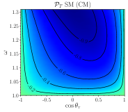
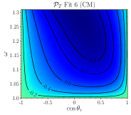
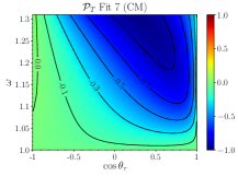
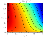
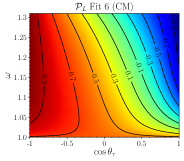
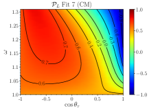
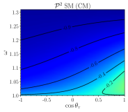
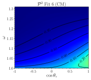
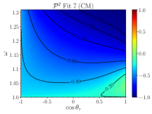
Figure 1: CM ${\cal P}_{T}$ (first row), ${\cal P}_{L}$ (second row) and ${\cal P}^{2}$ (third row) polarization observables for the $\Lambda_{b}\to\Lambda_{c}\tau\bar{\nu}_{\tau}$ decay evaluated within the SM (left column) and with the NP Wilson coefficients from Fits 6 (middle column) and 7 (right column) of Ref. Murgui:2019czp . We display the 2D distributions as a function of the $(\omega,\cos\theta_{\tau})$ variables. In all cases, central values for the form factors and Wilson coefficients have been used.

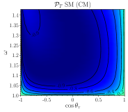
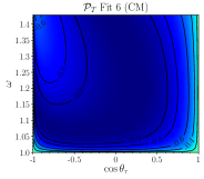
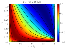
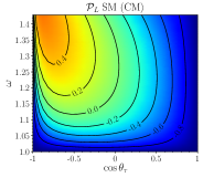
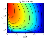
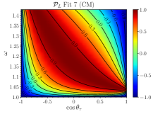
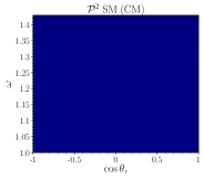
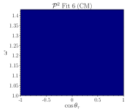
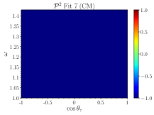
Figure 2: The same as in Fig. 1, but for the $\bar{B}\to D\tau\bar{\nu}_{\tau}$ decay.

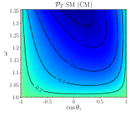
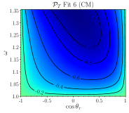
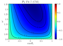
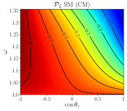
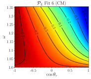
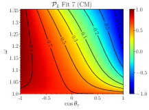
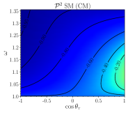
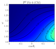
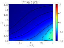
Figure 3: The same as in Fig. 1, but for the $\bar{B}\to D^{*}\tau\bar{\nu}_{\tau}$ decay.

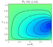
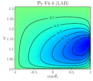
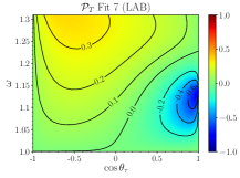
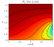
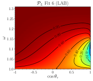
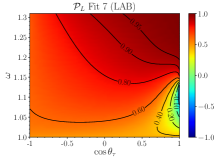
Figure 4: LAB ${\cal P}_{T}$ (first row) and ${\cal P}_{L}$ (second row) polarization observables for the $\Lambda_{b}\to\Lambda_{c}\tau\bar{\nu}_{\tau}$ decay evaluated within the SM (left column) and with the NP Wilson coefficients from Fits 6 (middle column) and 7 (right column) of Ref. Murgui:2019czp . We display the 2D distributions as a function of the $(\omega,\cos\theta_{\tau})$ variables, and use Eq. (32) to compute the $\cos\theta_{\tau}$ for fixed $\omega$ and a given $E_{\tau}$ LAB energy. In all cases, central values for the form factors and Wilson coefficients have been used.

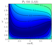
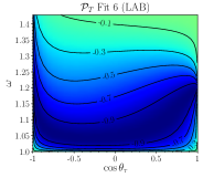
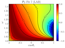
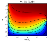
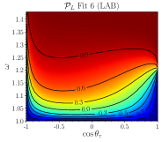
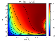
Figure 5: The same as in Fig. 4, but for the $\bar{B}\to D\tau\bar{\nu}_{\tau}$ decay.

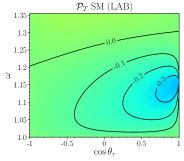
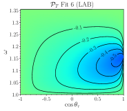
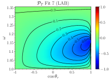
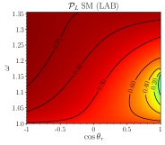
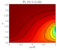
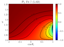
Figure 6: The same as in Fig. 4, but for the $\bar{B}\to D^{*}\tau\bar{\nu}_{\tau}$ decay.

Two-dimensional (2D) distributions of the ${\cal P}^{\mu}$ projections provide observables that can also be used to distinguish between different types of NP. In this subsection, we discuss results obtained within the SM and the NP scenarios corresponding to Fits 6 and 7 of Ref. Murgui:2019czp . Since in this latter work, all Wilson coefficients are real, the ${\cal P}_{TT}$ component comes out identically zero.

First in Figs. 1, 2 and 3, we show CM 2D distributions for ${\cal P}_{L}$, ${\cal P}_{T}$ and ${\cal P}^{2}$ and the $\Lambda_{b}\to\Lambda_{c}$, $\bar{B}\to D$ and $\bar{B}\to D^{*}$ decays, respectively, and obtained with the central values for the Wilson coefficients and form factors. In all cases, predictions from Fit 6 are closer to the SM results, and we clearly observe, except for the $\bar{B}\to D^{*}$ decay, different 2D patterns for Fits 6 and 7, which would certainly allow to distinguish between both NP scenarios.

The transverse component ${\cal P}_{T}$ is always negative for $\Lambda_{b}\to\Lambda_{c}$ and $\bar{B}\to D^{*}$ decays, with a $\cos\theta_{\tau}-$dependence that becomes flatter as $\omega$ decreases from $\omega_{\rm max}$ to the vicinity of zero recoil ($\omega=1$), where ${\cal P}_{T}$ reaches, in modulus, its minimum value. Large negative values of ${\cal P}_{T}$, which can reach $-0.9$, are found for $\omega>1.2$ and intermediate values of $\cos\theta_{\tau}$ far from the $\pm 1$ limits. For these two decays, the longitudinal polarization shows a large variation, going from ${\cal P}_{L}\sim 0.9$ for angles close to $\pi$ to values in the $(-0.9,-0.8)$ range in the forward direction, where the dependence on $\omega$ is significantly more pronounced than at backward angles. Moreover, we see regions close to zero recoil, and in the forward direction, where the $\tau-$lepton is produced largely unpolarized (${\cal P}^{2}\sim-0.2$), with $|{\cal P}^{2}\,|$ growing as both $\theta_{\tau}$ and $\omega$ increases, reaching values in the interval $(-0.95,-0.9)$ for $\omega$ in the vicinity of $\omega_{\max}$ (see the 2D$-{\cal P}^{2}$ distributions in the bottom panels). The exception is found for NP Fit 7 in the baryon decay, for which the $\tau$ is produced almost polarized, ${\cal P}^{2}<-0.95$ at forward angles and close to $\omega_{\rm max}$ (right-top corner), with a large ${\cal P}_{T}$ polarization component, around $-0.9$. However, in this case for backward angles, ${\cal P}^{2}$ does not become so close to $-1$ as $\omega$ approaches $\omega_{\rm max}$.

The discussion for the $\bar{B}\to D$ transition should take into account that for this decay ${\cal P}^{2}=-1$, implying that the $\tau$ emitted is always fully polarized. In Ref. Penalva:2020ftd , it was already pointed out that for $0^{-}\to 0^{-}$ transitions at zero recoil and $\theta_{\tau}=0$ or $\pi$, angular momentum conservation forces the $\tau$ helicity to equal that of the antineutrino which is positive, thus ${\cal P}_{L}=-1$ (see Eq. (34) or (35)), which implies ${\cal P}^{2}=-{\cal P}_{L}^{2}=-1$ and ${\cal P}_{T}=0$.

Indeed, we see in the bottom panels of Fig. 2 that ${\cal P}^{2}=-1$ in the whole $(\omega,\cos\theta_{\tau})$ phase-space, and not only for $\theta_{\tau}=0$ or $\pi$ at zero recoil. Therefore, longitudinal and transverse polarizations are not independent for non-CP violating physical scenarios, and in the full phase-space both components satisfy the relation ${\cal P}_{L}^{2}+{\cal P}_{T}^{2}=1$. As in the other decays, Fit 7 predictions differ from SM ones significantly more than those obtained in the NP Fit 6, with ${\cal P}_{L}$ exhibiting a pronounced dependence on $\cos\theta_{\tau}$, when $\omega$ departs from the zero recoil point. While ${\cal P}_{L}$ takes negative and positive values within the SM and both Fits 6 and 7 of Ref. Murgui:2019czp , we observe that ${\cal P}_{T}$ is negative for SM and Fit 6, while for the NP Fit 7, this transverse component also takes positive and negative values, and even it vanishes along a $(\omega,\cos\theta_{\tau})-$curve, for which ${\cal P}_{L}=+1$. As we will see below, for the kinematics encoded in this curve, the $\tau-$lepton is produced in a negative-helicity state.

The reason why the $\tau$ is always fully polarized for a general $0^{-}\to 0^{-}$ transition is the following. Since, in the massless limit, the $\bar{\nu}_{\tau}$ is fully polarized, we have that the invariant amplitude ${\cal M}$, apart from momenta, only depends on the $\tau$ spin degrees of freedom. If we have ${\cal M}(h)$, where here $h=\pm 1$ represents the $\tau$ helicity, one can always define two coefficients

$$a_{\pm 1}=\frac{\pm{\cal M}(h=\mp 1)}{\sum_{h^{\prime}=\pm 1}|{\cal M}(h^{\prime})|^{2}}$$ (44)

such that $\sum_{h=\pm 1}|a_{h}|^{2}=1$ and satisfy

$$\sum_{h=\pm 1}a_{h}{\cal M}(h)=0,\$$ (45)

What this result tells us is that the probability to produce a $\tau$ in the state $a^{*}_{+1}u^{\tilde{s}}_{+1}(k^{\prime})+a^{*}_{-1}u^{\tilde{s}}_{-1}(k^{\prime})$ is identically zero. Thus, the probability to produce a $\tau$ in the orthogonal state, $a_{-1}u^{\tilde{s}}_{+1}(k^{\prime})-a_{+1}u^{\tilde{s}}_{-1}(k^{\prime})$, should be one. The $\tau$ is then fully polarized. Apart from irrelevant phases these two polarization states correspond to

$$a^{*}_{+1}u^{\tilde{s}}_{+1}(k^{\prime})+a^{*}_{-1}u^{\tilde{s}}_{-1}(k^{\prime})\equiv u^{\cal P}_{+1}(k^{\prime}),\quad a_{-1}u^{\tilde{s}}_{+1}(k^{\prime})-a_{+1}u^{\tilde{s}}_{-1}(k^{\prime})\equiv u^{\cal P}_{-1}(k^{\prime}),$$ (46)

i.e., they are the two spin-covariant eigenstates associated to the four-vector $N^{\mu}={\cal P}^{\mu}$. For a given $k^{\prime}$, these states depend on the pair of variables $(\omega,\cos\theta_{\tau})$ or $(\omega,E_{\tau})$ that determine all ${\cal P}^{\mu}$ components (or equivalently ${\cal M}$) in the CM or LAB frames respectively. The above argumentation fails as soon as $\cal M$ depends on the spin variable of the hadrons involved in the decay. This is so since, in general, it is not possible to find $a_{\pm 1}$ such that

$$\sum_{h=\pm 1}a_{h}{\cal M}_{\lambda}(h)=0,$$ (47)

for all $\lambda\equiv(r,r^{\prime})$ values, where different $\lambda$ values represent different hadronic spin configurations. Note however that for a fixed $\lambda$ (corresponding to fixed $r/r^{\prime}$ polarization of the initial/final hadron) Eq. (47) has always a solution. Thus, for fixed $\lambda$, the $\tau$ is also fully polarized but with a polarization state that depends on $\lambda$. This is in agreement with the results obtained in Ref. Tanaka:1994ay for $\bar{B}\to D^{(*)}$ decays.

As noted above, for the rest of the transitions, ${\cal P}^{2}$ approaches $-1$ at maximum recoil ($\omega_{\rm max}$), with the exception of Fit 7 for the $\Lambda_{b}\to\Lambda_{c}$ decay in the $\cos\theta_{\tau}<0$ region. This is better understood by looking at the polarization projections in the laboratory frame.

In Figs. 4–6, we present the LAB ${\cal P}_{L}$ and ${\cal P}_{T}$ 2D distributions for the same NP scenarios and decays discussed previously in Figs. 1–3. In the LAB plots, we have made use of the relation in Eq. (32) to represent the polarization observables as a function of $(\omega,\cos\theta_{\tau})$ instead of $(\omega,E_{\tau})$. On the other hand, since ${\cal P}^{2}$ is a scalar [and thus ${\cal P}^{2}_{\rm LAB}(\omega,E_{\tau}(\omega,\cos\theta_{\tau}))={\cal P}^{2}_{\rm CM}(\omega,\cos\theta_{\tau})$ ] we will no show it again.

Though the LAB ${\cal P}_{L}$ and ${\cal P}_{T}$ 2D distributions shown in Figs. 4–6 can be obtained from the CM ones depicted above in Figs. 1–3, we stress that the coefficients of the linear combinations (Eq. (30)) depend on $\omega$ and $\cos\theta_{\tau}$. Moreover, the longitudinal or transverse character is not preserved, which also makes interesting a short discussion of the main features of the LAB polarization components. In the LAB frame, the $\tau$’s are mainly being emitted with negative helicity (${\cal P}_{L}^{\rm LAB}\approx 1$) in the high $\omega$-region close to $\omega_{\rm max}$, as can be seen in the second row of plots in Figs. 4–6. The explanation for this behavior, at least in part, is that close to maximum recoil, the $\tau$ momentum in the LAB is large and hence positive helicity is suppressed by the dominant contribution that selects negative chirality for the final charged lepton. As mentioned in Ref. Penalva:2020ftd , only the ${\cal O}_{S_{L},S_{R}}$ and ${\cal O}_{T}$ NP terms select positive chirality. Looking at the values for the corresponding Wilson coefficients (see Table 6 of Ref. Murgui:2019czp ) one expects larger deviations from the above behavior for Fit 7.

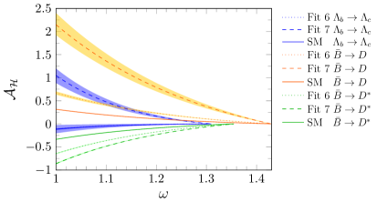
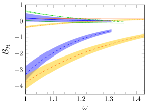
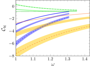
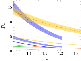
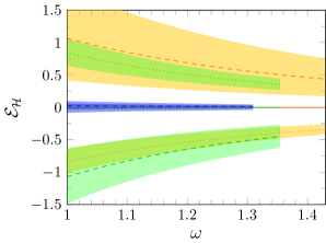
Figure 7: ${\cal A_{H}}(\omega)$, ${\cal B_{H}}(\omega)$, ${\cal C_{H}}(\omega)$, ${\cal D_{H}}$ and ${\cal E_{H}}(\omega)$ functions (Eqs. (21) and (23)) for the $\Lambda_{b}\to\Lambda_{c}$ (bluish), $\bar{B}\to D$ (reddish) and $\bar{B}\to D^{*}$ (greenish) decays evaluated for the SM (solid), Fit 6 (dotted) and Fit 7 (dashed) of Ref. Murgui:2019czp . Error bands take into account the uncertainties associated to the Wilson coefficients and form factors, and they are calculated as explained in Refs. Penalva:2020xup ; Penalva:2020ftd .

To finish this subsection, we recall here that for fixed $\omega$, the polarization components turn out to be ratios of linear or quadratic functions of $(p\cdot k)$, as inferred from Eqs. (33) and (37). Restricting the discussion to CM observables, the denominator of these ratios, ${\cal N}(\omega,p\cdot k)$, is proportional to $p_{\cal N}(\omega,\cos\theta_{\tau})=a_{0}(\omega)+a_{1}(\omega)\cos\theta_{\tau}+a_{2}(\omega)\cos^{2}\theta_{\tau}$, with the coefficients $a_{i}(\omega)$ appearing in the angular decomposition of the tau-unpolarized $d^{2}\Gamma/(d\omega d\cos\theta_{\tau})$ differential decay width. We have already presented results for them in our previous works Penalva:2020xup ; Penalva:2020ftd , and we will not make any further comment here. On the other hand, taking into account the dependence of $(p\cdot k),(p\cdot N_{L,T}^{\rm CM})$ and $(q\cdot N_{L,T}^{\rm CM})$ on $\cos\theta_{\tau}$, we find

$$P_{L}^{\rm CM}(\omega,\cos\theta_{\tau}) = \frac{p_{0}(\omega)+p_{1}(\omega)\cos\theta_{\tau}+p_{2}(\omega)\cos^{2}\theta_{\tau}}{a_{0}(\omega)+a_{1}(\omega)\cos\theta_{\tau}+a_{2}(\omega)\cos^{2}\theta_{\tau}},$$

$$P_{T}^{\rm CM}(\omega,\cos\theta_{\tau}) = \sin\theta_{\tau}\frac{p^{\prime}_{0}(\omega)+p^{\prime}_{1}(\omega)\cos\theta_{\tau}}{a_{0}(\omega)+a_{1}(\omega)\cos\theta_{\tau}+a_{2}(\omega)\cos^{2}\theta_{\tau}}$$ (48)

with the five coefficients, $p_{0},p_{1},p_{2},p^{\prime}_{0}$ and $p^{\prime}_{1}$, of the numerator polynomials being linear combination of the five ${\cal A_{H}}(\omega)$, ${\cal B_{H}}(\omega)$, ${\cal C_{H}}(\omega)$, ${\cal D_{H}}$ and ${\cal E_{H}}(\omega)$ functions, introduced in Eqs. (21) and (23) to generally describe the decay with polarized taus in the final state. We observe that $P_{L}^{\rm CM}$ and $P_{T}^{\rm CM}$ are not just polynomials in $\cos\theta_{\tau}$ and that the simultaneous knowledge/measure of both of them, in conjunction with the unpolarized $d^{2}\Gamma/(d\omega d\cos\theta_{\tau})$ distribution, provide the maximum information which can be obtained from the decay with polarized taus. In addition, the longitudinal component, or equivalently the CM tau-helicity $d^{2}\Gamma/(d\omega d\cos\theta_{\tau})$ double differential decay width, provides only three independent conditions ($p_{0},p_{1}$ and $p_{2}$) and it is not enough to determine all undetermined ${\cal A_{H}},\cdots{\cal E_{H}}$ functions. This was already pointed out in Ref. Penalva:2020xup , where it is also shown that all these functions can be obtained using also input from the LAB tau-helicity $d^{2}\Gamma/(d\omega dE_{\tau})$ distribution (or equivalently $P_{L}^{\rm LAB}$), as expected from the discussion in Eq. (30) since this brings in some information of $P_{T}^{\rm CM}$. This is another way to point out that the CM and LAB tau-helicity differential distributions provide complementary results.

Thus, we show results for ${\cal A_{H}}(\omega)$, ${\cal B_{H}}(\omega)$, ${\cal C_{H}}(\omega)$, ${\cal D_{H}}$ and ${\cal E_{H}}(\omega)$, since this is another, more simple, way of presenting the physical information contained in the above 2D polarization observables. This is done in Fig.7 for the $\Lambda_{b}\to\Lambda_{c}\tau\bar{\nu}_{\tau}$ and $\bar{B}\to D^{(*)}\tau\bar{\nu}_{\tau}$ decays. We note that these functions could also be reconstructed from the exhaustive results included in Refs. Penalva:2020xup ; Penalva:2020ftd on the tau CM angular and LAB energy dependencies of the helicity $d^{2}\Gamma/(d\omega d\cos\theta_{\tau})$ and $d^{2}\Gamma/(d\omega dE_{\tau})$ distributions, but that they have never been directly shown. In most cases we see the capability of these observables to distinguish the SM and Ref. Murgui:2019czp Fits 6 and 7 predictions, with the latter deviating more from the SM results. One can have direct access to these functions by measuring the $\tau$ polarization in the decay or, indirectly, through the measuring of the polarization vectors components ${\cal P}_{L,T}$. The latter can be obtained for instance from the analysis of the subsequent $\tau$ decay. Both methods require however to be able to measure the $\tau$ momentum (in the first case also its polarization), something that it is extremely difficult, since the decay products of the tau include an undetected neutrino.

In this sense, we should comment that the framework presented in Refs. Asadi:2020fdo ; Alonso:2017ktd for $\bar{B}-$decays, where so-called visible distributions of detectable particles from the $\tau$-decay are analyzed, aims to determine the ${\cal A_{H}},\cdots{\cal E_{H}}$ functions without having to measure the $\tau$ momentum. Indeed, it is integrated out in these works, and the proposed (visible) kinematical variables are referred to the initial $\bar{B}$ and outgoing $D^{(*)}$ three-momenta. Further and complementary constrains, within this scheme of visible kinematics, can also be obtained from different angular asymmetries that can be constructed using the products of the final hadron decay ($D^{*}\to D\pi$) Bhattacharya:2020lfm .

4.2 One-dimensional polarization averages

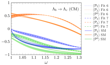
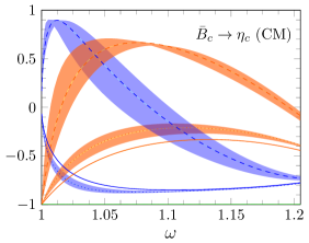
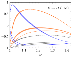
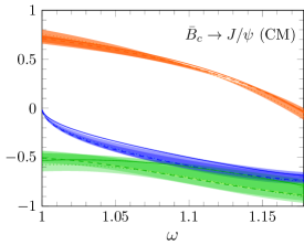
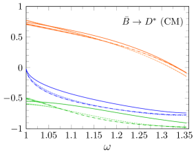
Figure 8: Polarization $\langle{\cal P}_{T}^{\rm CM}\rangle$, $\langle{\cal P}_{L}^{\rm CM}\rangle$ and $\langle{\cal P}^{2}\rangle$ averages, defined in the CM system and calculated for the SM and the NP Fits 6 and 7 of Ref. Murgui:2019czp , as a function of $\omega$. In addition, for the $\bar{B}\to D$ decay, the gray curves stand for the SM (solid), Fit 6 (dotted) and Fit 7 (dashed) results obtained for $-|\vec{P}_{\rm CM}|^{2}$ (Eq. (43)). Error bands take into account the uncertainties associated to the Wilson coefficients and form factors, and they are calculated as explained in Refs. Penalva:2020xup ; Penalva:2020ftd .

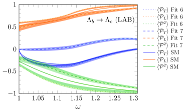
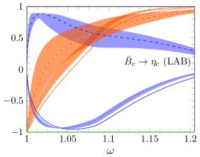
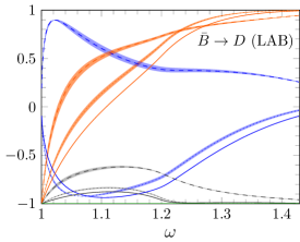
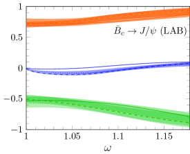
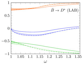
Figure 9: The same as in Fig. 8, but for projections defined in the LAB system.

Some of the features discussed above in the presentation of the ${\cal P}_{L,T}$ results are easier to observe in the one dimensional plots displayed in Figs. 8 and 9. There, we now show the CM and LAB $\langle{\cal P}_{L}\rangle(\omega)$, $\langle{\cal P}_{T}\rangle(\omega)$ and $\langle{\cal P}^{2}\rangle(\omega)$ averages, the latter given by $\langle{\cal P}^{2}\rangle(\omega)=-\langle{\cal P}^{2}_{L}+{\cal P}^{2}_{T}+{\cal P}^{2}_{TT}\rangle(\omega)$, as introduced in Eqs. (39) and (41). As discussed in Subsec. 3.2, these averages are related to the CM/LAB tau polarization asymmetries obtained from $d\Gamma/d\omega$, whose measurement require the detection of the momentum and spin-state of the $\tau$. Equivalently, these averages can be obtained from the analysis of the full angular distribution of the pion or rho mesons, originated in the subsequent hadron decay of the tau, measured in the $\tau$-rest frame Ivanov:2017mrj . Following the discussion at the end of the previous subsection, these observables seem more difficult to access experimentally than those proposed in Refs. Asadi:2020fdo ; Alonso:2017ktd , which do not require the detection of the tau lepton and that we will study elsewhere.

In Figs. 8 and 9, only NP Fits 6 and 7 of Ref. Murgui:2019czp are still considered, where all Wilson coefficients are real and therefore the ${\cal P}_{TT}$ component vanishes. Additionally, we also show results for the $\bar{B}_{c}\to\eta_{c}\tau\bar{\nu}_{\tau}$ and $\bar{B}_{c}\to J/\psi\tau\bar{\nu}_{\tau}$ decays, not presented for the 2D distributions and the ${\cal A_{H}},\cdots{\cal E_{H}}$ functions discussed in the previous subsection. We include, in all cases, 68% confident-level (CL) error bands that take into account the uncertainties associated to the Wilson coefficients and form factors, as explained in Refs. Penalva:2020xup ; Penalva:2020ftd .

The $\omega-$shape patterns for the $\bar{B}\to D$ and $\bar{B}_{c}\to\eta_{c}$ or the $\bar{B}\to D^{*}$ and $\bar{B}_{c}\to J/\psi$ reactions are qualitatively similar, while those obtained from the $\Lambda_{b}\to\Lambda_{c}$ decay show some resemblances with the $0^{-}\to 1^{-}$ ones. A good number of the distributions depicted in Figs. 8 and 9 can be used to disentangle between SM and the two NP cases considered there. In particular, Fit 7 leads to results clearly distinctive, even taking into account theoretical uncertainties bands, while SM and Fit 6 predictions are more difficult to separate. Nevertheless, from the results of Figs. 8 and  9 one can safely conclude that, with the exception of the $\bar{B}_{c}\to J/\psi$, and to a lesser extent $\bar{B}\to D^{*}$, the observables shown could theoretically tell apart Fit 6 from Fit 7.

We note that the averages of the LAB longitudinal and transverse projections $\langle{\cal P}_{L,T}^{\rm LAB}\rangle(\omega)$ can not be obtained as linear combinations of the $\langle{\cal P}_{L,T}^{\rm CM}\rangle(\omega)$ with known kinematical coefficients. They provide thus complementary information. This is easily seen in the expressions collected in Appendix B. In addition to ${\cal A},{\cal B}$ and ${\cal C}$, which could be extracted from either the unpolarized CM $d^{2}\Gamma/(d\omega d\cos\theta_{\tau})$ or the LAB $d^{2}\Gamma/(d\omega dE_{\tau})$ differential decay widths Penalva:2020xup , we observe that $\langle{\cal P}_{T}^{\rm CM}\rangle(\omega)$ depends on ${\cal A_{H}}$ and ${\cal C_{H}}$ while, in $\langle{\cal P}_{L}^{\rm CM}\rangle(\omega)$, the scalar $\omega$-functions ${\cal B_{H}}$, ${\cal D_{H}}$ and ${\cal E_{H}}$ also appear. In turn, $\langle{\cal P}_{T}^{\rm LAB}\rangle$ provides an independent linear combination of ${\cal B_{H}}$, ${\cal D_{H}}$ and ${\cal E_{H}}$, and the expression for $\langle{\cal P}_{L}^{\rm LAB}\rangle(\omega)$ involves all the ${\cal A_{H}}$, ${\cal B_{H}}$, ${\cal C_{H}}$, ${\cal D_{H}}$ and ${\cal E_{H}}$ functions. Another consequence of this discussion is that for a given decay, all former five $\omega$-functions cannot be determined only from the four averages $\langle{\cal P}_{L,T}^{\rm CM}\rangle(\omega)$ and $\langle{\cal P}_{L,T}^{\rm LAB}\rangle(\omega)$, and it would be necessary to have additional information, as for example the two-dimensional dependencies of the different polarization components discussed in the previous subsection. Alternatively, as noted above, all these scalars (${\cal A_{H}},\cdots{\cal E_{H}}$) can also be obtained from the combined study of the CM $d^{2}\Gamma/(d\omega d\cos\theta_{\tau})$ and LAB $d^{2}\Gamma/(d\omega dE_{\tau})$ helicity-polarized distributions Penalva:2020xup .

However, it is clear that the combined use of all averages, for the five decays, shown in Figs. 8 and 9 will greatly restrict the characteristics of possible extensions of the SM, and certainly in a more efficient way than if only one particular decay is considered.

Finally, for the $\bar{B}\to D$ decay, we also show (gray curves and bands) the frame dependent quantity $-|\vec{P}|^{2}$ (see Eq. (43)), introduced in Ref. Ivanov:2017mrj . Clearly, $-|\vec{P}|^{2}$ fails to convey the information on the degree of polarization of the $\tau$. For the $\bar{B}\to D$ decay, and except at zero recoil, for which $-|\vec{P}|^{2}=-\langle{\cal P}_{L}\rangle^{2}=\langle{\cal P}^{2}\rangle=-1$, its value is never exactly minus one. We also test that while $\langle{\cal P}^{2}\rangle$ is a scalar and leads to the same LAB and CM $\omega$-distributions, $-|\vec{P}|^{2}$ depends on the reference system where it has been defined. We observe that in the high $\omega$-region, $-|\vec{P}|^{2}$ in LAB is closer to $-1$ than when it is calculated in CM, being in the first frame almost indistinguishable from $-1$ for the SM and Fit 6 cases. This follows from the discussion above of the LAB 2D distributions, where we pointed out that ${\cal P}_{L}$ approaches 1 at maximum recoil, as a consequence of an approximate negative-helicity selection by the dominant operators in that $\omega$ region (large $\tau$ LAB momentum).

4.2.1 Complex Wilson coefficients

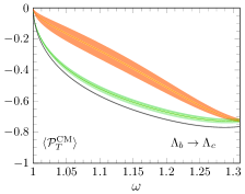
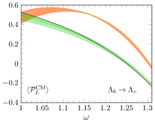
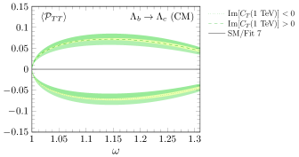
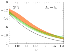
Figure 10: Polarization averages $\langle{\cal P}_{T}^{\rm CM}\rangle(\omega)$, $\langle{\cal P}_{L}^{\rm CM}\rangle(\omega)$, $\langle{\cal P}_{TT}^{\rm CM}\rangle(\omega)$ and $\langle{\cal P}^{2}\rangle(\omega)$ defined in the CM system and calculated for the SM (black) and the NP Wilson coefficients from Fit 7 (red) of Ref. Murgui:2019czp and the $R_{2}$ leptoquark model fit (green) of Ref. Shi:2019gxi (see text for details). Error bands take into account the uncertainties associated to the Wilson coefficients and form factors, and they are calculated as explained in the main text for the $R_{2}$ leptoquark model fit, and in Ref. Penalva:2020xup for the SM and Fit 7.

For the particular case of the $\Lambda_{b}\to\Lambda_{c}$ transition, we also show in Fig. 10 results for the $R_{2}$ leptoquark model fit of Ref. Shi:2019gxi . This fit is particularly interesting since the two nonzero Wilson coefficients, $C_{S_{L}}$ and $C_{T}$, are complex giving rise to a nonzero $\langle{\cal P}_{TT}^{\rm CM}\rangle(\omega)$ value. For this particular model $C_{S_{L}}$ and $C_{T}$ at the bottom mass scale, appropriate for the present calculation, are given in terms of just the value of $\hat{C}_{T}$ at the scale of 1 TeV, with $\hat{C}_{S_{L}}(1\,\rm{TeV})=4\,\hat{C}_{T}(1\,\rm{TeV})$, and the corresponding evolution matrix (see Ref. Shi:2019gxi ). The right panel of figure 4 of Ref. Shi:2019gxi shows the constraints on the complex $C_{S_{L}}$ plane, with best fit point at $C_{S_{L}}=-0.08\pm 0.30~{}i$. As we have done in Figs. 8 and 9, the error on the observables inherited from the form-factor uncertainties is evaluated and propagated via Monte Carlo, taking into account statistical correlations between the different parameters. It is shown as an inner error band that accounts for 68% CL intervals. The uncertainty induced by the fitted Wilson coefficients is determined using different $1\sigma$ Wilson coefficients configurations provided by the authors of Ref. Shi:2019gxi . The two sets of errors are then added in quadrature giving rise to the larger uncertainty band that can be seen in the figure.

In Fig. 10, and for the sake of comparison, we also include the polarization observables obtained with the SM and Fit 7 of Ref. Murgui:2019czp . We do not show in the figure any result for Fit 6 of Murgui:2019czp , because this latter NP fit leads to predictions close to the SM ones.

The results for $\langle{\cal P}_{L,T}\rangle$ obtained with the $R_{2}$ fit of Ref. Shi:2019gxi are closer to the SM ones than the ones obtained from Fit 7 of Ref. Murgui:2019czp . This is particularly true for $\langle{\cal P}_{L}\rangle$ where the SM result is contained in the error band of the $R_{2}-$model prediction. Things change for $\langle{\cal P}_{TT}\rangle$. As mentioned above, the complex $C_{S_{L}}$ and $C_{T}$ Wilson coefficients of the $R_{2}$ fit of Ref. Shi:2019gxi generate a nonzero average-polarization $\langle{\cal P}_{TT}\rangle(\omega)$, which is shown in the lower-left panel of Fig. 10. The nonzero-result for $\langle{\cal P}_{TT}\rangle$ comes from the interference of SM vector-axial with the NP terms, as well as the interference between the NP terms themselves. While for the $R_{2}$ model most observables are quadratic in the imaginary part of $\hat{C}_{T}(1\,{\rm TeV})$, like $\langle{\cal P}^{\rm CM}_{L,T}\rangle$ here but also the ${\cal R}_{D^{(*)}},\ {\cal R}_{\Lambda_{c}},{\cal R}_{J/\psi}$ ratios, and the $\tau$ ($A_{\lambda_{\tau}}$) and the longitudinal $D^{*}$ ($F_{L}^{D^{*}}$) polarization asymmetries, $\langle{\cal P}_{TT}\rangle$ is indeed linear in the imaginary part of $\hat{C}_{T}(1\,{\rm TeV})$. This allows to break the degeneracy present in the other observables with respect to the sign of ${\rm Im\,}[\hat{C}_{T}(1\,{\rm TeV})]$.

As discussed above, the projection ${\cal P}_{TT}$ is invariant under co-linear boost transformations, and as a consequence the LAB average $\langle{\cal P}_{TT}\rangle(\omega)$ would be identical to that shown in Fig. 10, and evaluated in the CM frame. This average can be used to determine the linear combination of the functions ${\cal F_{H}}$ and ${\cal G_{H}}$ given in Eq. (57) of the appendix. However, additional information on the CM angular dependence of the ${\cal P}_{TT}$ projection would be required to separately extract the time-reversal odd functions ${\cal F_{H}}$ and ${\cal G_{H}}$. The experimental finding of signatures of non-zero tau polarization in a direction perpendicular to the plane formed by the CM (or LAB) three momenta of the outgoing hadron and the $\tau$ would be a clear indication, not only of NP beyond the SM, but also of CP (or time reversal) violation.

The results for ${\cal R}_{\Lambda_{c}}$ are collected in Table 1. The result obtained with the $R_{2}$ fit of Ref. Shi:2019gxi is not far from to the SM one. Part of the reason for this behavior could be in the use, in Ref. Shi:2019gxi , of $B\to D^{(*)}$ form factors evaluated in the heavy quark limit. The use of the improved form factors obtained in Ref. Murgui:2019czp , which included sub-leading corrections, in the $R_{2}$ fit gives rise to a larger ${\rm Im\,}[\hat{C}_{T}(1\,{\rm TeV})]$ value that results in ${\cal R}_{\Lambda_{c}}$ being larger around $\sim 0.385$.

	SM	Fit 7 Murgui:2019czp	$R_{2}$ Shi:2019gxi
$\Gamma_{e(\mu)}/\left(10\times|V_{cb}|^{2}{\rm ps}^{-1}\right)$	$2.15\pm 0.08$	$-$	$-$
$\Gamma_{\tau}/\left(10\times|V_{cb}|^{2}{\rm ps}^{-1}\right)$	$0.715\pm 0.015$	$0.89\pm 0.05$	$0.75\pm 0.02$
${\cal R}_{\Lambda_{c}}$	$0.332\pm 0.007$	$0.41\pm 0.02$	$0.350\pm 0.010$

Table 1: Total decay widths $\Gamma_{\tau}=\Gamma\left(\Lambda_{b}\to\Lambda_{c}\tau\bar{\nu}_{\tau}\right)$ and $\Gamma_{e(\mu)}=\Gamma\left(\Lambda_{b}\to\Lambda_{c}\,e(\mu)\bar{\nu}_{e(\mu)}\right)$ and ratios ${\cal R}_{\Lambda_{c}}=\Gamma\left(\Lambda_{b}\to\Lambda_{c}\tau\bar{\nu}_{\tau}\right)/\Gamma\left(\Lambda_{b}\to\Lambda_{c}\,e(\mu)\bar{\nu}_{e(\mu)}\right)$ obtained in the SM and in the NP scenarios corresponding to Fit 7 of Ref. Murgui:2019czp and the $R_{2}$ leptoquark model fit of Ref. Shi:2019gxi (see text for details).

5 Summary

For a given configuration of the momenta of all particles involved, we have introduced the tau spin-density matrix $\bar{\rho}$ and the polarization vector ${\cal P}^{\mu}$ associated to a general $H_{b}\to H_{c}\tau\bar{\nu}_{\tau}$ decay. These two quantities contain all the information on the spin state of the $\tau$ provided no other particle spin is measured. For different semileptonic decays, we have evaluated ${\cal P}^{\mu}$ in the LAB and CM frames including the effects of NP. We have seen that the independent components ${\cal P}_{L}$, ${\cal P}_{T}$ and ${\cal P}_{TT}$ provide useful information to distinguish between different NP scenarios. This is specially true for the meson $0^{-}\to 0^{-}$ and also for the baryon $\Lambda_{b}\to\Lambda_{c}$ reactions analyzed in this work. For this latter reaction, we have presented results for an extension of the SM that contains complex Wilson coefficients.

The LAB and CM helicity-polarized differential decay widths do not allow access to observables related to ${\cal P}_{TT}$, which is the component of the polarization vector orthogonal to the plane defined by the final hadron and tau three-momenta. Moreover, ${\cal P}_{T}$, which is the projection of $\vec{{\cal P}}$ contained in the former plane and perpendicular to the $\tau-$momentum, can only be obtained indirectly from these helicity-distributions, provided that results from both reference systems are analyzed simultaneously. The transverse polarization ${\cal P}_{TT}$ is of special interest, since it is only possible for complex Wilson coefficients. Measuring a non-zero ${\cal P}_{TT}$ value in any of the two frames will be a clear indication of physics beyond the SM and of time reversal (or CP) violation. For the NP scenarios corresponding to Fits 6 and 7 of Ref. Murgui:2019czp the Wilson coefficients are real and thus ${\cal P}_{TT}$ is identically zero. In such a case, $\vec{\cal P}$ is contained in the hadron-lepton plane. The $R_{2}$ fit of Ref. Shi:2019gxi , which contains $C_{S_{L}}$ and $C_{T}$ complex Wilson coefficients generates, however, a nonzero ${\cal P}_{TT}$ value.

The NP effective Hamiltonian in Eq. (15) contains five Wilson coefficients, in general complex, although one of them can always be taken to be real. Therefore, nine free parameters should be determined from data. Even assuming that the form factors are known, and therefore the genuinely hadronic part ($W$) of the $\widetilde{W}$ SFs, it is difficult to determine all NP parameters from a unique type of decay, since the experimental measurement of the required polarization observables is an extremely difficult task. It is therefore essential to simultaneously analyze data from various types of semileptonic decays, as we have done in this work. We have used state of the art form-factors for all reactions, and the results presented in this work nicely complement those presented in our previous works of Refs. Penalva:2020xup ; Penalva:2020ftd , and all together can be efficiently employed to disentangle among different NP scenarios.

Finally, we would like to draw the attention to the hadron-tensor method used in this work, previously derived in Penalva:2020xup , which has shown to be a particularly suited tool to study processes where all final/initial hadron polarizations have been summed up. The scheme leads to compact expressions, valid for any baryon/meson semileptonic decay for unpolarized hadrons in the presence of NP and it clearly is an alternative to the helicity amplitude framework commonly used in the literature. Subsequent decays of the produced $\tau$, after the $b\to c\tau\bar{\nu}_{\tau}$ transition,

$$H_{b}\to H_{c} \tau^{-} \bar{\nu}_{\tau}$$ (49)

$$\,\drsh \nu_{\tau}\mu^{-}\bar{\nu}_{\mu},\,\nu_{\tau}\pi^{-},\,\nu_{\tau}\rho^{-}\,\cdots$$

can be straightforwardly studied within this hadron-tensor scheme and they will be presented elsewhere.

Appendix A CM and LAB kinematics

In this appendix we collect the different vector products needed to evaluate the ${\cal P}_{L},\,{\cal P}_{T}$ and ${\cal P}_{TT}$ polarization vector components in the CM and LAB reference frames. We have

$$p^{2}=M^{2},\,\,k^{2}=0,\,\,k^{\prime 2}=m^{2}_{\tau},\,\,p\cdot q=MM_{\omega},\,\,k\cdot k^{\prime}=q\cdot k=\frac{q^{2}-m^{2}_{\tau}}{2},\,\,q\cdot k^{\prime}=\frac{q^{2}+m^{2}_{\tau}}{2},$$ (50)

with $M_{\omega}=M-M^{\prime}\omega$. In addition, the scalar products that depend explicitly on the charged lepton variables used in the differential decay widths read

LAB: In this case, $p^{\mu}=(M,\vec{0}\,)$, $q^{\mu}=\left(M_{\omega},\,M^{\prime}\sqrt{\omega^{2}-1}\,\hat{q}_{\rm LAB}\right)$ and

$$k\cdot p=M(M_{\omega}-E_{\tau}),\quad p\cdot N_{L}=\frac{M\sqrt{E^{2}_{\tau}-m^{2}_{\tau}}}{m_{\tau}},\quad p\cdot N_{T}=0,$$

$$q\cdot N_{L}=\frac{M_{\omega}\sqrt{E_{\tau}^{2}-m_{\tau}^{2}}}{m_{\tau}}+\frac{E_{\tau}\,M^{\prime}\sqrt{\omega^{2}-1}}{m_{\tau}}\,\cos\theta_{\tau}^{\rm LAB},\quad q\cdot N_{T}=M^{\prime}\sqrt{\omega^{2}-1}\,\sin\theta_{\tau}^{\rm LAB},$$

$$\epsilon^{k^{\prime}q\,p\,N_{TT}}=-MM^{\prime}\sqrt{\omega^{2}-1}\,\sqrt{E^{2}_{\tau}-m^{2}_{\tau}}\,\sin\theta_{\tau}^{\rm LAB},$$ (51)

with $\theta_{\tau}^{\rm LAB}$ the angle made by the final hadron and $\tau$ lepton LAB three-momenta, which is fixed, once $E_{\tau}$ and $\omega$ are known, by the relation

$$\cos\theta_{\tau}^{\rm LAB}=\frac{q^{2}+m^{2}_{\tau}-2M_{\omega}E_{\tau}}{2M^{\prime}\sqrt{\omega^{2}-1}\,\sqrt{E^{2}_{\tau}-m^{2}_{\tau}}}.$$ (52)

For a given $\omega$, the fact that $|\cos\theta_{\tau}^{\rm LAB}|\leq 1$ limits the possible $E_{\tau}$ energies to the interval

$$E_{\tau}\in[E_{\tau}^{-}(\omega),\,E_{\tau}^{+}(\omega)],$$ (53)

with $E_{\tau}^{-}$ and $E_{\tau}^{+}$ given in Eq. (36). In terms of $E_{\tau}^{\pm}(\omega)$ one also can write

$$\sin\theta_{\tau}^{\rm LAB}=\frac{\sqrt{q^{2}}\sqrt{\big{[}E_{\tau}-E_{\tau}^{-}(\omega)\big{]}\big{[}E_{\tau}^{+}(\omega)-E_{\tau}\big{]}}}{M^{\prime}\sqrt{\omega^{2}-1}\sqrt{E_{\tau}^{2}-m_{\tau}^{2}}}.$$ (54)

CM: Now $q^{\mu}=(\sqrt{q^{2}},\vec{0}\,)$ and $p^{\mu}=\frac{1}{\sqrt{q^{2}}}\left(MM_{\omega},\,-MM^{\prime}\sqrt{\omega^{2}-1}\,\hat{q}_{\rm LAB}\right)$, and in addition

$$k\cdot p=\frac{M}{2}\left(1-\frac{m^{2}_{\tau}}{q^{2}}\right)\left(M_{\omega}+M^{\prime}\sqrt{\omega^{2}-1}\cos\theta_{\tau}\right),\ \ q\cdot N_{L}=\frac{q^{2}-m^{2}_{\tau}}{2m_{\tau}},\ \ q\cdot N_{T}=0,$$

$$p\cdot N_{L}=\frac{MM_{\omega}(q^{2}-m^{2}_{\tau})-MM^{\prime}\sqrt{\omega^{2}-1}\,(q^{2}+m^{2}_{\tau})\cos\theta_{\tau}}{2m_{\tau}q^{2}},$$

$$p\cdot N_{T}=-\frac{MM^{\prime}\sqrt{\omega^{2}-1}}{\sqrt{q^{2}}}\,\sin\theta_{\tau},$$

$$\epsilon^{k^{\prime}q\,p\,N_{TT}}=-MM^{\prime}\sqrt{\omega^{2}-1}\,\frac{q^{2}-m^{2}_{\tau}}{2\sqrt{q^{2}}}\sin\theta_{\tau}.$$ (55)

Note that, since the three-vector components transverse to the velocity defining a boost do not change, we obtain

$$\sqrt{E^{2}_{\tau}-m^{2}_{\tau}}\,\sin\theta_{\tau}^{\rm LAB}=|\vec{k}^{\,\prime\,}|^{\rm LAB}\sin\theta_{\tau}^{\rm LAB}=|\vec{k}^{\,\prime\,}|^{\rm CM}\sin\theta_{\tau}=\frac{q^{2}-m^{2}_{\tau}}{2\sqrt{q^{2}}}\sin\theta_{\tau}$$ (56)

and then $\epsilon^{k^{\prime}q\,p\,N_{TT}}\big{|}_{\rm LAB}=\epsilon^{k^{\prime}q\,p\,N_{TT}}\big{|}_{\rm CM}$, which shows that ${\cal P}_{TT}^{\rm LAB}={\cal P}_{TT}^{\rm CM}$, since the other factor ${\cal N_{H_{\rm 3}}}(\omega,\,k\cdot p)/{\cal N}(\omega,\,k\cdot p)$ in Eq. (38) is a Lorentz scalar.

Appendix B Expressions for $\langle{\cal P}_{L,T,TT}^{\rm CM}\rangle(\omega)$ and $\langle{\cal P}_{L,T,TT}^{\rm LAB}\rangle(\omega)$

In this appendix we give expressions for $\langle{\cal P}_{L,T,TT}^{\rm CM,\,LAB}\rangle(\omega)$ in terms of the ten scalar functions, ${\cal A},{\cal B}$, ${\cal C}$, ${\cal A_{H}},{\cal B_{H}},{\cal C_{H}},{\cal D_{H}}$, ${\cal E_{H}}$, ${\cal F_{H}}$ and ${\cal G_{H}}$, introduced in Eq. (21). One has

$$\langle{\cal P}_{L}^{\rm CM}\rangle(\omega) = -\frac{1}{m_{\tau}}\frac{1}{M{\cal N}_{\theta}(\omega)}\left(1-\frac{m^{2}_{\tau}}{q^{2}}\right)\left[MM_{\omega}{\cal A_{H}}(\omega)+q^{2}{\cal B_{H}}(\omega)+\frac{M_{\omega}\left(q^{2}-m^{2}_{\tau}\right)}{2M}{\cal D_{H}}(\omega)\right.$$

$$+ \left.\frac{{\cal C_{H}}(\omega)}{6}\left(q^{2}+m^{2}_{\tau}+2M_{\omega}^{2}-\frac{4m^{2}_{\tau}M^{2}_{\omega}}{q^{2}}\right)-\frac{\left(q^{2}-m^{2}_{\tau}\right)^{2}}{12M^{2}q^{2}}\left(q^{2}-4M_{\omega}^{2}\right){\cal E_{H}}(\omega)\right],$$

$$\langle{\cal P}_{T}^{\rm CM}\rangle(\omega) = \frac{\pi M^{\prime}}{{\cal N}_{\theta}(\omega)}\frac{\sqrt{\omega^{2}-1}}{4\sqrt{q^{2}}}\left[2{\cal A_{H}}(\omega)+\frac{M_{\omega}}{M}\left(1-\frac{m^{2}_{\tau}}{q^{2}}\right){\cal C_{H}}(\omega)\right],$$

$$\langle{\cal P}_{TT}^{\rm CM}\rangle(\omega) = -\frac{\pi M^{\prime}}{{\cal N}_{\theta}(\omega)}\frac{\sqrt{\omega^{2}-1}}{8\sqrt{q^{2}}}\left(1-\frac{m^{2}_{\tau}}{q^{2}}\right)\left[\frac{2q^{2}}{M^{2}}{\cal F_{H}}(\omega)+\frac{M_{\omega}(q^{2}-m^{2}_{\tau})}{M^{3}}{\cal G_{H}}(\omega)\right],$$ (57)

with

$${\cal N}_{\theta}(\omega)={\cal A}(\omega)+\left(1-\frac{m^{2}_{\tau}}{q^{2}}\right)\left[\frac{M_{\omega}}{2M}{\cal B}(\omega)+\left(1-\frac{m^{2}_{\tau}}{q^{2}}\right)\left(\frac{4M_{\omega}^{2}-q^{2}}{12M^{2}}\right){\cal C}(\omega)\right].$$ (58)

Note that from Eq. (40), $\langle{\cal P}_{L}^{\rm CM}\rangle(\omega)$ can be written as

$$\langle{\cal P}_{L}^{\rm CM}\rangle(\omega)=\frac{[a_{0}(\omega,h=-1)-a_{0}(\omega,h=1)]+\frac{1}{3}[a_{2}(\omega,h=-1)-a_{2}(\omega,h=1)]}{a_{0}(\omega)+\frac{1}{3}a_{2}(\omega)}$$ (59)

where the $a_{0,2}(\omega)$ and $a_{0,2}(\omega,h=\pm 1)$ functions are given in Eqs. (18) and (25) of Ref. Penalva:2020xup in terms of the eight ${\cal A}(\omega)$,  ${\cal B}(\omega)$, ${\cal C}(\omega)$, ${\cal A_{H}}(\omega)$, ${\cal B_{H}}(\omega)$, ${\cal C_{H}}(\omega)$, ${\cal D_{H}}(\omega)$ and ${\cal C_{H}}(\omega)$ ones.

In the LAB frame one has that,

$$\langle{\cal P}_{L}^{\rm LAB}\rangle(\omega) = \frac{1}{\left(E_{\tau}^{+}-E_{\tau}^{-}\right)\,{\cal N}_{\theta}(\omega)}$$ (60)

$$\times \bigg{\{}M\hat{c}_{0}(\omega)\,\ln\left(\frac{E_{\tau}^{+}+p_{\tau}^{+}}{E_{\tau}^{-}+p_{\tau}^{-}}\right)+\left(c_{0}(\omega)+\hat{c}_{1}(\omega)\right)\left(p_{\tau}^{+}-p_{\tau}^{-}\right)$$

$$+ \frac{c_{1}(\omega)+\hat{c}_{2}(\omega)}{2M}\Big{[}E_{\tau}^{+}p_{\tau}^{+}-E_{\tau}^{-}p_{\tau}^{-}+m_{\tau}^{2}\,\ln\left(\frac{E_{\tau}^{+}+p_{\tau}^{+}}{E_{\tau}^{-}+p_{\tau}^{-}}\right)\Big{]}$$

$$+ \frac{c_{2}(\omega)+\hat{c}_{3}(\omega)}{3M^{2}}\Big{[}\left(E_{\tau}^{+\,2}+2m_{\tau}^{2}\right)p_{\tau}^{+}-\left(E_{\tau}^{-\,2}+2m_{\tau}^{2}\right)p_{\tau}^{-}\Big{]}\bigg{\}},$$

with $p_{\tau}^{\pm}(\omega)=\sqrt{\left[E_{\tau}^{\pm}(\omega)\right]^{2}-m_{\tau}^{2}}$ and where $\hat{c}_{0}(\omega)$, $\left(c_{0}(\omega)+\hat{c}_{1}(\omega)\right)$, $\left(c_{1}(\omega)+\hat{c}_{2}(\omega)\right)$ and $\left(c_{2}(\omega)+\hat{c}_{3}(\omega)\right)$ are given in Eq. (27) of Ref. Penalva:2020xup in terms of the ${\cal A_{H}}(\omega)$,  ${\cal B_{H}}(\omega)$, ${\cal C_{H}}(\omega)$, ${\cal D_{H}}(\omega)$ and ${\cal E_{H}}(\omega)$ functions. Besides,

$$\langle{\cal P}_{T}^{\rm LAB}\rangle(\omega) = -\frac{\pi\sqrt{q^{2}}M^{\prime}\sqrt{\omega^{2}-1}}{4{\cal N}_{\theta}(\omega)M^{2}\left(1-\frac{m^{2}_{\tau}}{q^{2}}\right)}\bigg{[}\Big{(}\frac{4I_{0}(\omega)M_{\omega}}{M_{\omega}+\sqrt{q^{2}}}-I_{1}(\omega)\Big{)}{\cal D_{H}}(\omega)+$$

$$\frac{4I_{0}(\omega)M}{M_{\omega}+\sqrt{q^{2}}}{\cal B_{H}}(\omega)+\Big{(}\frac{8I_{0}(\omega)M_{\omega}}{M_{\omega}+\sqrt{q^{2}}}+I_{2}(\omega)-4I_{1}(\omega)\Big{)}\frac{M_{\omega}}{2M}{\cal E_{H}}(\omega)\bigg{]}$$

$$\langle{\cal P}_{TT}^{\rm LAB}\rangle(\omega) = \langle{\cal P}_{TT}^{\rm CM}\rangle(\omega),$$ (61)

where we have introduced the (kinematical) functions $I_{0,1,2}(\omega)$,

$$I_{n}(\omega) = \frac{1}{K_{n}}\int_{E_{\tau}^{-}(\omega)}^{E_{\tau}^{+}(\omega)}\frac{dE_{\tau}\,E_{\tau}^{n}}{\sqrt{E_{\tau}^{2}-m^{2}_{\tau}}}\sqrt{\left(E_{\tau}^{+}(\omega)-E_{\tau}\right)\left(E_{\tau}-E_{\tau}^{-}(\omega)\right)},\quad n=0,1,2$$

$$K_{0} = \frac{\pi}{2}\left(M_{\omega}-\sqrt{q^{2}}\right),\quad K_{1}=\frac{\pi}{8}\left(M_{\omega}^{2}-q^{2}\right),\quad K_{2}=\frac{\pi M_{\omega}}{16}\left(M_{\omega}^{2}-q^{2}\right)$$ (62)

which are normalized such that $I_{0}=I_{1}=I_{2}=1$ in the $m_{\tau}\to 0$ limit.

The formulae are general and they can be also used for muon or electron decay modes, taking appropriate values for the NP Wilson coefficients.

References

- (1) HFLAV collaboration, Averages of -hadron, -hadron, and -lepton properties as of 2018, 1909.12524.
- (2) BaBar collaboration, Evidence for an excess of decays, Phys. Rev. Lett. 109 (2012) 101802 [1205.5442].
- (3) BaBar collaboration, Measurement of an Excess of Decays and Implications for Charged Higgs Bosons, Phys. Rev. D88 (2013) 072012 [1303.0571].
- (4) Belle collaboration, Measurement of the branching ratio of relative to decays with hadronic tagging at Belle, Phys. Rev. D92 (2015) 072014 [1507.03233].
- (5) Belle collaboration, Measurement of the branching ratio of relative to decays with a semileptonic tagging method, Phys. Rev. D94 (2016) 072007 [1607.07923].
- (6) Belle collaboration, Measurement of the lepton polarization and in the decay , Phys. Rev. Lett. 118 (2017) 211801 [1612.00529].
- (7) Belle collaboration, Measurement of and with a semileptonic tagging method, Phys. Rev. Lett. 124 (2020) 161803 [1910.05864].
- (8) LHCb collaboration, Measurement of the ratio of branching fractions , Phys. Rev. Lett. 115 (2015) 111803 [1506.08614].
- (9) LHCb collaboration, Measurement of the ratio of the and branching fractions using three-prong -lepton decays, Phys. Rev. Lett. 120 (2018) 171802 [1708.08856].
- (10) S. Aoki et al., Review of lattice results concerning low-energy particle physics, Eur. Phys. J. C77 (2017) 112 [1607.00299].
- (11) D. Bigi and P. Gambino, Revisiting , Phys. Rev. D94 (2016) 094008 [1606.08030].
- (12) D. Bigi, P. Gambino and S. Schacht, , , and the Heavy Quark Symmetry relations between form factors, JHEP 11 (2017) 061 [1707.09509].
- (13) S. Jaiswal, S. Nandi and S.K. Patra, Extraction of from and the Standard Model predictions of , JHEP 12 (2017) 060 [1707.09977].
- (14) F.U. Bernlochner, Z. Ligeti, M. Papucci and D.J. Robinson, Combined analysis of semileptonic decays to and : , , and new physics, Phys. Rev. D95 (2017) 115008 [1703.05330].
- (15) S. Iguro and R. Watanabe, Bayesian fit analysis to full distribution data of determination and new physics constraints, JHEP 08 (2020) 006 [2004.10208].
- (16) A.K. Alok, D. Kumar, S. Kumbhakar and S. Uma Sankar, Solutions to - in light of Belle 2019 data, Nucl. Phys. B 953 (2020) 114957 [1903.10486].
- (17) S. Kumbhakar, Signatures of complex new physics in transitions, Nucl. Phys. B 963 (2021) 115297 [2007.08132].
- (18) R. Alonso, B. Grinstein and J. Martin Camalich, Lifetime of Constrains Explanations for Anomalies in , Phys. Rev. Lett. 118 (2017) 081802 [1611.06676].
- (19) LHCb collaboration, Measurement of the ratio of branching fractions /, Phys. Rev. Lett. 120 (2018) 121801 [1711.05623].
- (20) A.Y. Anisimov, I.M. Narodetsky, C. Semay and B. Silvestre-Brac, The meson lifetime in the light front constituent quark model, Phys. Lett. B452 (1999) 129 [hep-ph/9812514].
- (21) M.A. Ivanov, J.G. Korner and P. Santorelli, Exclusive semileptonic and nonleptonic decays of the meson, Phys. Rev. D73 (2006) 054024 [hep-ph/0602050].
- (22) E. Hernández, J. Nieves and J. Verde-Velasco, Study of exclusive semileptonic and non-leptonic decays of - in a nonrelativistic quark model, Phys. Rev. D 74 (2006) 074008 [hep-ph/0607150].
- (23) T. Huang and F. Zuo, Semileptonic decays and charmonium distribution amplitude, Eur. Phys. J. C51 (2007) 833 [hep-ph/0702147].
- (24) W. Wang, Y.-L. Shen and C.-D. Lu, Covariant Light-Front Approach for B(c) transition form factors, Phys. Rev. D79 (2009) 054012 [0811.3748].
- (25) W.-F. Wang, Y.-Y. Fan and Z.-J. Xiao, Semileptonic decays in the perturbative QCD approach, Chin. Phys. C37 (2013) 093102 [1212.5903].
- (26) R. Watanabe, New Physics effect on in relation to the anomaly, Phys. Lett. B 776 (2018) 5 [1709.08644].
- (27) A. Issadykov and M.A. Ivanov, The decays and in covariant confined quark model, Phys. Lett. B783 (2018) 178 [1804.00472].
- (28) C.-T. Tran, M.A. Ivanov, J.G. Körner and P. Santorelli, Implications of new physics in the decays , Phys. Rev. D97 (2018) 054014 [1801.06927].
- (29) X.-Q. Hu, S.-P. Jin and Z.-J. Xiao, Semileptonic decays in the ”PQCD + Lattice” approach, Chin. Phys. C44 (2020) 023104 [1904.07530].
- (30) D. Leljak, B. Melic and M. Patra, On lepton flavour universality in semileptonic decays, JHEP 05 (2019) 094 [1901.08368].
- (31) K. Azizi, Y. Sarac and H. Sundu, Lepton flavor universality violation in semileptonic tree level weak transitions, Phys. Rev. D99 (2019) 113004 [1904.08267].
- (32) W. Wang and R. Zhu, Model independent investigation of the and ratios of decay widths of semileptonic decays into a P-wave charmonium, Int. J. Mod. Phys. A 34 (2019) 1950195 [1808.10830].
- (33) P. Colangelo, F. De Fazio and F. Loparco, Role of in the Standard Model and in the search for BSM signals, Phys. Rev. D 103 (2021) 075019 [2102.05365].
- (34) D. Bečirević, F. Jaffredo, A. Peñuelas and O. Sumensari, New Physics effects in leptonic and semileptonic decays, 2012.09872.
- (35) S. Bhattacharya, S. Nandi and S. Kumar Patra, Decays: a catalogue to compare, constrain, and correlate new physics effects, Eur. Phys. J. C 79 (2019) 268 [1805.08222].
- (36) C. Murgui, A. Peñuelas, M. Jung and A. Pich, Global fit to transitions, JHEP 09 (2019) 103 [1904.09311].
- (37) R.-X. Shi, L.-S. Geng, B. Grinstein, S. Jäger and J. Martin Camalich, Revisiting the new-physics interpretation of the data, JHEP 12 (2019) 065 [1905.08498].
- (38) HFLAV collaboration, Averages of -hadron, -hadron, and -lepton properties as of summer 2016, Eur. Phys. J. C77 (2017) 895 [1612.07233].
- (39) M. Duraisamy and A. Datta, The Full Angular Distribution and CP violating Triple Products, JHEP 09 (2013) 059 [1302.7031].
- (40) M. Duraisamy, P. Sharma and A. Datta, Azimuthal angular distribution with tensor operators, Phys. Rev. D 90 (2014) 074013 [1405.3719].
- (41) D. Becirevic, S. Fajfer, I. Nisandzic and A. Tayduganov, Angular distributions of decays and search of New Physics, Nucl. Phys. B 946 (2019) 114707 [1602.03030].
- (42) P. Colangelo and F. De Fazio, Scrutinizing and in search of new physics footprints, JHEP 06 (2018) 082 [1801.10468].
- (43) Z. Ligeti, M. Papucci and D.J. Robinson, New Physics in the Visible Final States of , JHEP 01 (2017) 083 [1610.02045].
- (44) B. Bhattacharya, A. Datta, S. Kamali and D. London, A measurable angular distribution for decays, JHEP 07 (2020) 194 [2005.03032].
- (45) T. Gutsche, M.A. Ivanov, J.G. Körner, V.E. Lyubovitskij, P. Santorelli and N. Habyl, Semileptonic decay in the covariant confined quark model, Phys. Rev. D 91 (2015) 074001 [1502.04864].
- (46) K. Azizi and J.Y. Süngü, Semileptonic Transition in Full QCD, Phys. Rev. D 97 (2018) 074007 [1803.02085].
- (47) F.U. Bernlochner, Z. Ligeti, D.J. Robinson and W.L. Sutcliffe, New predictions for semileptonic decays and tests of heavy quark symmetry, Phys. Rev. Lett. 121 (2018) 202001 [1808.09464].
- (48) S. Shivashankara, W. Wu and A. Datta, Decay in the Standard Model and with New Physics, Phys. Rev. D 91 (2015) 115003 [1502.07230].
- (49) A. Ray, S. Sahoo and R. Mohanta, Probing new physics in semileptonic decays, Phys. Rev. D99 (2019) 015015 [1812.08314].
- (50) X.-Q. Li, Y.-D. Yang and X. Zhang, decay in scalar and vector leptoquark scenarios, JHEP 02 (2017) 068 [1611.01635].
- (51) A. Datta, S. Kamali, S. Meinel and A. Rashed, Phenomenology of using lattice QCD calculations, JHEP 08 (2017) 131 [1702.02243].
- (52) M. Blanke, A. Crivellin, S. de Boer, T. Kitahara, M. Moscati, U. Nierste et al., Impact of polarization observables and on new physics explanations of the anomaly, Phys. Rev. D99 (2019) 075006 [1811.09603].
- (53) F.U. Bernlochner, Z. Ligeti, D.J. Robinson and W.L. Sutcliffe, Precise predictions for semileptonic decays, Phys. Rev. D99 (2019) 055008 [1812.07593].
- (54) E. Di Salvo, F. Fontanelli and Z.J. Ajaltouni, Detailed Study of the Decay , Int. J. Mod. Phys. A33 (2018) 1850169 [1804.05592].
- (55) M. Blanke, A. Crivellin, T. Kitahara, M. Moscati, U. Nierste and I. Nišandžić, Addendum to 2̆01cImpact of polarization observables and on new physics explanations of the anomaly”, Phys. Rev. D100 (2019) 035035 [1905.08253].
- (56) P. Böer, A. Kokulu, J.-N. Toelstede and D. van Dyk, Angular Analysis of , 1907.12554.
- (57) M. Ferrillo, A. Mathad, P. Owen and N. Serra, Probing effects of new physics in decays, 1909.04608.
- (58) P. Colangelo, F. De Fazio and F. Loparco, Inclusive semileptonic decays in the Standard Model and beyond, JHEP 11 (2020) 032 [2006.13759].
- (59) N. Penalva, E. Hernández and J. Nieves, Further tests of lepton flavour universality from the charged lepton energy distribution in semileptonic decays: The case of , Phys. Rev. D100 (2019) 113007 [1908.02328].
- (60) N. Penalva, E. Hernández and J. Nieves, Hadron and lepton tensors in semileptonic decays including new physics, Phys. Rev. D 101 (2020) 113004 [2004.08253].
- (61) N. Penalva, E. Hernández and J. Nieves, , and semileptonic decays including new physics, Phys. Rev. D 102 (2020) 096016 [2007.12590].
- (62) M. Tanaka, Charged Higgs effects on exclusive semitauonic decays, Z. Phys. C 67 (1995) 321 [hep-ph/9411405].
- (63) U. Nierste, S. Trine and S. Westhoff, Charged-Higgs effects in a new B — D tau nu differential decay distribution, Phys. Rev. D 78 (2008) 015006 [0801.4938].
- (64) M. Tanaka and R. Watanabe, New physics in the weak interaction of , Phys. Rev. D 87 (2013) 034028 [1212.1878].
- (65) M.A. Ivanov, J.G. Körner and C.-T. Tran, Probing new physics in using the longitudinal, transverse, and normal polarization components of the tau lepton, Phys. Rev. D 95 (2017) 036021 [1701.02937].
- (66) R. Alonso, J. Martin Camalich and S. Westhoff, Tau properties in from visible final-state kinematics, Phys. Rev. D 95 (2017) 093006 [1702.02773].
- (67) P. Asadi, A. Hallin, J. Martin Camalich, D. Shih and S. Westhoff, Complete framework for tau polarimetry in decays, Phys. Rev. D 102 (2020) 095028 [2006.16416].
- (68) J.G. Korner and G.A. Schuler, Exclusive Semileptonic Heavy Meson Decays Including Lepton Mass Effects, Z. Phys. C46 (1990) 93.
- (69) L. Zhang, X.-W. Kang, X.-H. Guo, L.-Y. Dai, T. Luo and C. Wang, A comprehensive study on the semileptonic decay of heavy flavor mesons, JHEP 02 (2021) 179 [2012.04417].
- (70) LHCb collaboration, Measurement of the shape of the differential decay rate, Phys. Rev. D96 (2017) 112005 [1709.01920].
- (71) Particle Data Group collaboration, Review of Particle Physics, PTEP 2020 (2020) 083C01.
- (72) F. Mandl and G. Shaw, QUANTUM FIELD THEORY, Wiley, Chichester (1985).
- (73) C. Itzykson and J.B. Zuber, Quantum Field Theory, International Series In Pure and Applied Physics, McGraw-Hill, New York (1980).
- (74) LATTICE-HPQCD collaboration, and Lepton Flavor Universality Violating Observables from Lattice QCD, Phys. Rev. Lett. 125 (2020) 222003 [2007.06956].
- (75) D. Bečirević, I. Doršner, S. Fajfer, N. Košnik, D.A. Faroughy and O. Sumensari, Scalar leptoquarks from grand unified theories to accommodate the -physics anomalies, Phys. Rev. D 98 (2018) 055003 [1806.05689].
- (76) W. Detmold, C. Lehner and S. Meinel, and form factors from lattice QCD with relativistic heavy quarks, Phys. Rev. D92 (2015) 034503 [1503.01421].
- (77) Fermilab Lattice, MILC collaboration, Update of from the form factor at zero recoil with three-flavor lattice QCD, Phys. Rev. D 89 (2014) 114504 [1403.0635].
- (78) Fermilab Lattice and MILC collaboration, form factors at nonzero recoil and from 2+1-flavor lattice QCD, Phys. Rev. D92 (2015) 034506 [1503.07237].
- (79) HPQCD collaboration, form factors at nonzero recoil and extraction of , Phys. Rev. D92 (2015) 054510 [1505.03925].
- (80) HPQCD collaboration, Lattice QCD calculation of the form factors at zero recoil and implications for , Phys. Rev. D 97 (2018) 054502 [1711.11013].
- (81) S. Faller, A. Khodjamirian, C. Klein and T. Mannel, Form Factors from QCD Light-Cone Sum Rules, Eur. Phys. J. C 60 (2009) 603 [0809.0222].
- (82) M. Neubert, Z. Ligeti and Y. Nir, QCD sum rule analysis of the subleading Isgur-Wise form-factor , Phys. Lett. B 301 (1993) 101 [hep-ph/9209271].
- (83) M. Neubert, Z. Ligeti and Y. Nir, The Subleading Isgur-Wise form-factor to order in QCD sum rules, Phys. Rev. D 47 (1993) 5060 [hep-ph/9212266].
- (84) Z. Ligeti, Y. Nir and M. Neubert, The Subleading Isgur-Wise form-factor and its implications for the decays , Phys. Rev. D 49 (1994) 1302 [hep-ph/9305304].
- (85) HPQCD collaboration, form factors for the full range from lattice QCD, Phys. Rev. D 102 (2020) 094518 [2007.06957].