HED-UNet: Combined Segmentation and Edge Detection for Monitoring the Antarctic Coastline

Abstract

This work has been accepted by IEEE TGRS for publication. Deep learning-based coastline detection algorithms have begun to outshine traditional statistical methods in recent years. However, they are usually trained only as single-purpose models to either segment land and water or delineate the coastline. In contrast to this, a human annotator will usually keep a mental map of both segmentation and delineation when performing manual coastline detection. To take into account this task duality, we therefore devise a new model to unite these two approaches in a deep learning model. By taking inspiration from the main building blocks of a semantic segmentation framework (UNet) and an edge detection framework (HED), both tasks are combined in a natural way. Training is made efficient by employing deep supervision on side predictions at multiple resolutions. Finally, a hierarchical attention mechanism is introduced to adaptively merge these multiscale predictions into the final model output. The advantages of this approach over other traditional and deep learning-based methods for coastline detection are demonstrated on a dataset of Sentinel-1 imagery covering parts of the Antarctic coast, where coastline detection is notoriously difficult. An implementation of our method is available at https://github.com/khdlr/HED-UNet.

I Introduction

Contrary to many other landmasses, Antarctica’s coastline is fringed by dynamic glacier and ice shelf fronts continuously changing the coastline location by iceberg calving, which is influenced by both seasonal variations as well as global climate change. Tracking the advance and retreat of glacier and ice shelf fronts is an important factor for a better understanding of glaciological processes. Furthermore, it is essential to monitor calving front retreat as it enhances the sea level contribution of the Antarctic ice sheet due to decreased buttressing effects.

Overall, the length of the Antarctic coastline amounts to around $40\,000\text{\,}\mathrm{km}$ [1], which renders manual delineation infeasible. Especially when observing the developments over multiple time steps for continuous tracking, an automated coastline extraction technique is needed. The recent advances in algorithms and sensing platforms open up new possibilities for the analysis of satellite imagery over large regions, which can be observed in fields as diverse as land cover mapping [2, 3, 4], bathymetry [5, 6, 7], urban applications [8, 9, 10, 11, 12], change detection [13, 14, 15, 16, 17], and cryosphere research [18, 19, 20, 21, 22].

This kind of fine-grained analysis is possible because of the availability of satellite imagery with revisit times in the order of days. Regarding data sources, both optical and synthetic aperture radar (SAR) sensors produce imagery suitable for the delineation of the Antarctic coastline [23]. The use of optical imagery in the Antarctic comes with some major drawbacks. Apart from the usual problems with cloud cover, vision is further impeded by polar night and sensor saturation due to the high albedo of ice. To create continuous and gapless observations, data from the Sentinel-1 mission was chosen as the main imagery source. SAR data has often been found to be helpful with the analysis of the cryosphere [24, 25, 26, 27, 28, 29, 30, 31, 32, 33]. In our case, it allows for near-realtime analysis at a high temporal resolution.

Using SAR data for the task of coastline extraction also imposes some challenges. The speckle present in SAR images makes it harder to pinpoint the exact boundary between land and sea. Further, the backscatter characteristics of glacial ice vary throughout the year, making it hard to distinguish between e. g. open sea and the higher ice sheet. Therefore, a good model needs to pay additional attention to contextual clues and cannot rely on local information only.

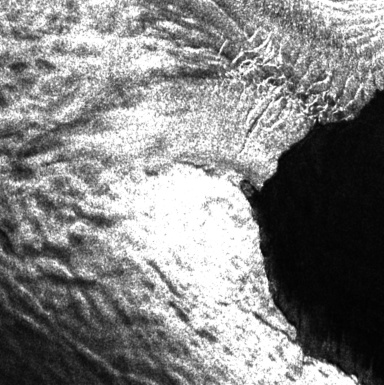
SAR imagery Segmentation Edge Detection

Figure 1: In coastline detection, the vision tasks of segmentation and edge detection are inseparable.

Existing studies for delineating coastlines in general, as well as the Antarctic one, often focus their predictions on either the area of land and sea (sea-land segmentation), or the coastline itself (coastline detection). But to the human eye, the two concepts of “area” and “edge” are closely intertwined, making it hard to imagine one without the other. When conducting manual coastline delineation, a human annotator will therefore mentally segment the scene into sea and land while searching for the edge between the two at the same time.

We hypothesize that taking into account this duality is essential in closing the performance gap between human annotators and automated approaches. In an attempt to more closely model this process, we thus introduce a new solution for coastline detection that draws upon the advantages of both segmentation and edge detection approaches. Instead of focusing a predictor on just one of these tasks, our network is trained to jointly perform both tasks at the same time. Inspired by neural architectures for semantic segmentation and edge detection, the model uses an encoder-decoder architecture with skip connections in order to predict segmentation masks and edges at multiple resolutions.

Another observation we make about coastline detection conducted by humans is the fact that not all areas of a given scene need the same amount of attention to detail. While it is of paramount importance that the coastal regions are precisely mapped, areas further away from the coastline do not receive much attention from a human annotator. By introducing a merging scheme based on hierarchical attention, our model can work in the same way. The intermediate multiresolution predictions are merged using this mechanism to obtain a final output that combines fine-grained low level outputs with coarser high level outputs in an efficient way.

Overall, this work’s contributions are threefold:

• Coastline detection is recognized as a dual task. To solve this, a unified theory of segmentation and edge detection is presented. From this, an architecture that implements both semantic segmentation and edge detection is devised.

• Apart from the narrow coastal strip, there are large regions that require less detailed analysis. This is taken into account by allowing the model to output predictions at different resolution levels. Adding deep supervision for these side outputs improves the training efficiency and generalization performance of the model.

• In order to dynamically blend between coarse and high-resolution predictions, a hierarchical attention mechanism is used that takes into account the information available at all levels.

The remainder of the paper is organized as follows. Section II gives a brief overview of current methods for coastline detection with a focus on polar regions, as well as existing approaches for combining segmentation and edge detection. Section III presents our proposed HED-UNet architecture. In Section IV, the used dataset is introduced. Further, the conducted experiments are explained. Finally, Section V presents numerical results comparing our model to other approaches and ablation studies that analyze the proposed model’s elements in detail. Finally, it also includes a discussion of the observed model performance.

II Related Work

This section will explore the state of the art for coastline detection with a focus on Antarctica. Compared to the general case, the detection of coastlines in the Antarctic requires additional care, as many methods are easily distracted by dynamic sea ice, like icebergs or ice mélange. Locally, these confounding features can look almost identical to land ice, and can therefore only be excluded by the additional use of spatial context information.

There are numerous existing approaches for detecting coastlines from satellite imagery. For the biggest part, they can be divided into the aforementioned two classes, differing in the output of interest.

II-A Sea-Land Segmentation

In the field of computer vision, semantic segmentation is a central topic. Each pixel is assigned a class which is to be predicted by the model. This technique is frequently used in remote sensing for various tasks. When the area of either sea or land is of importance, semantic segmentation models are used to distinguish between sea pixels and land pixels.

II-A1 Statistical Methods

In quite a few studies, this has been done by means of statistical analysis. For the Antarctic, the use of a bimodal Gaussian mixture model was proposed, for which parameters are estimated in order to derive an adaptive thresholding scheme. This approach can be applied to both SAR and optical imagery [1]. Similar dynamic thresholding schemes have been applied to different sensors [34]. While easy to implement and fast to evaluate, these methods completely discard the spatial relationships of the pixels, which renders them unfit to deal with the aforementioned issues.

Another localized way of segmenting images that has been applied to sea-land segmentation is given by the watershed algorithm [35]. It treats the pixel intensities as height values and then simulates the resulting surface being flooded with water. Finally, unsupervised clustering methods are helpful in the analysis of complex coastlines [36]. These methods have the benefit of being unsupervised, i. e. requiring no training prior to the evaluation, but the lack of supervision also means that the models cannot be taught to e. g. ignore icebergs.

II-A2 Deep Learning Methods

With the rise of deep learning in remote sensing [37], convolutional neural networks (CNNs) have been shown to provide superior performance for many tasks, including the one of sea-land segmentation [38, 39, 40]. Deep convolutional architectures like SegNet [41] or UNet [42] leverage contextual information through their encoder-decoder architectures. So as they have more context to base their decisions on, they have the potential to produce more accurate results than pixelwise or shallow texture-based classifiers. This is of great interest to Antarctic coastline detection due to the aforementioned issues. Current developments in computer vision show a trend towards more complex models for semantic segmentation, which incorporate global information [43] or shape information [44].

Generally, these models require large amounts of labeled data, and take quite some time to train. However, they can outperform the previously mentioned methods.

II-B Coastline Detection

A closely related task is approached in coastline detection. Instead of segmenting a scene into sea and land, the coastline itself is of primary interest.

II-B1 Edge Tracing

One class of edge detection methods mark the boundaries in the image step by step. After some filtering to highlight the edges, which can be done e. g. using the Roberts operator [45] or the Sobel operator [46], pixels that are likely to lie on the edge are connected to form the entire boundary. Regarding coastline detection, this approach has been shown to work for SAR data, when applying preprocessing steps to account for the nature of the imagery [47]. They can also be connected using a shortest-path algorithm [29], or ridge tracing [48]. Yet another approach comes from exploiting detection duality. By the nature of the relation between sea, land and the coastline, the coastline can be derived from a sea-land segmentation by tracing the transitions between the sea and land class [49].

While relatively simple, these methods often have some issues regarding robustness. When the tracing procedure takes a wrong turn, it is hard for the algorithm to return to the true boundary.

II-B2 Contour Methods

Active contours, sometimes also called Snakes [50], are quite similar to the edge tracing approach. Instead of the pixel-by-pixel approach, this class of methods uses an initial curve that is iteratively deformed to minimize an energy function. By choosing the right energy function, this framework can be used to delineate coastlines. For SAR imagery, active contours are able to find coastlines when given a good initialization [51, 52]. These models are sensitive to the provided initialization, meaning that they can converge to local minima that do not represent the desired edge.

II-B3 Level Set Methods

Instead of working with an explicit parametrization of the curve, these methods work with an implicit representation given by a scalar field in which the zero set represents the boundary [53, 54]. Adaptations of this method for SAR coastline detection use multiple level set iterations to go from coarse to fine delineations [55] or sophisticated preprocessing steps [56] to make the method work for this particular type of imagery.

II-B4 Deep Learning Methods

Only recently have approaches based on deep learning begun to outperform handcrafted edge detection algorithms. Specialized architectures leverage the framework of CNNs to derive features that predict the presence of edges [57, 58, 59]. Notably, the previously mentioned Roberts and Sobel operators can be viewed as a shallow CNNs with just one layer and a convolutional filter size of 2 and 3 respectively. Therefore, it is only natural that deeper CNNs with more layers are able to outperform these hardcoded edge detection operators.

II-C Combining Semantic Segmentation and Edge Detection

A common problem with semantic segmentation models is the blurriness near class boundaries. This likely stems from the fact that the edges make up a minority of the pixels, and are therefore not well enough represented by the standard pixelwise cross-entropy loss. Thus, the idea of augmenting semantic segmentation approaches with edge information is not a new one.

One way of making a segmentation model aware of edges in the image is by adding an auxiliary loss term that encourages the prediction of crisp edges. This has been shown to work for sea-land segmentation [60].

Surprisingly, simply adding the edge detection task as an auxiliary output for a segmentation model can improve the segmentation results quite a bit, even without further changes to the model [61]. This approach can also improve sea-land segmentation results in harbor areas [62].

To further improve blurry segmentations, edge masks can be used as the basis for a spatial propagation of class labels. In [63], a segmentation map is initialized using a segmentation network and at the same time, edges are predicted. These edge masks are then used as the basis for a recursive multidirectional label propagation.

For aerial scene classification, the use of an edge detection subnetwork before doing the segmentation has been shown to be beneficial. The detected edge masks are then used as additional input features for the segmentation model. This approach improves the shape accuracy of the resulting segmentation [64].

Contrary to these approaches, we develop a unified theory of segmentation and edge detection. We then identify the components that successful neural networks use to solve either one of these tasks, and finally devise a model that incorporates the tools necessary to solve both tasks at the same time. The underlying assumption is that both segmentation and edge detection are of equivalent importance for detecting coastlines in satellite imagery.

III Proposed Method

Implementing the sea-land segmentation task via a UNet segmentation model [42] has become a popular approach for the automatic delineation of coastlines [38, 39, 40]. And also on our dataset, this method yields good results on the majority of the evaluated scenes [31]. But oftentimes the predictions become inaccurate and blurry in areas close to the coastline. As the precise location of the coastline is the central object of our study,

On the other hand, edge detection models excel at delineating the edges in the given images. However, an edge delineation has no concept of “inside” and “outside” by itself, so this output alone is insufficient for labeling sea and land. Further, edge detection models are easily fooled by inland structures of similar appearance to the coastline, as well as icebergs near the coast. This implies the need for extensive post-processing and manual corrections.

To put our aforementioned hypotheses into practice, we now introduce a hybrid model for simultaneous prediction of the sea-land segmentation and edge detection of the coastline. Following our observation that humans will usually take into account both the edge information as well as the textural shape information, we therefore propose a combined framework that draws upon the advantages of both these approaches. It takes inspiration from both UNet [42] and HED [57], as well as related architectures by combining key ideas in a very natural way. Therefore, we call our model HED-UNet.

III-A Unifying Segmentation and Edge Detection

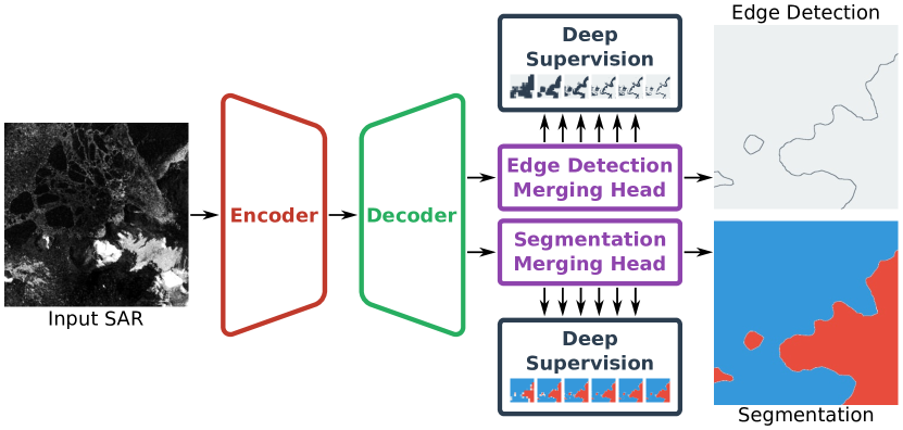
Figure 2: High-level structure of the proposed framework. First, the encoder and decoder calculate a pyramid of feature maps. Then, the task-specific merging heads combine this information using the hierarchical attention mechanism.

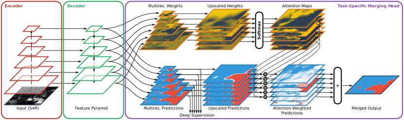
Figure 3: Architectural details of the proposed network. The full model contains two task-specific merging heads, for clarity, only the segmentation head is shown here. The edge detection head follows the same structure.

Regarding the deep learning formulation of the tasks, both segmentation and edge detection are in their nature dense prediction tasks, i. e. for each input pixel, an output label needs to be predicted. In the case of segmentation, this is the class label, like “sea” or “land”. For edge detection, it is a classification into the two classes “edge” and “no edge”.

This means that, in principle, a segmentation model can be trained to perform edge detection and vice versa. However, these models were designed for their respective tasks only, meaning the performance will be degraded when applying them to a different task. In order to construct a model that works well for both tasks, we will therefore identify the components of successful architectures for both tasks, and find a way to incorporate them into a single multitask model.

III-A1 Segmentation Building Blocks

Some successful semantic segmentation architectures employ the combination of an encoder and a decoder [42, 41]. The encoder conducts a series of downsampling steps to allow for the aggregation of contextual information at a lower resolution. In turn, the decoder then distributes this information to the individual pixels through a series of upsampling steps.

In a more recent branch of semantic segmentation approaches, the network architecture is divided into a backbone network that calculates feature maps, and one or multiple prediction heads, which conduct the final classification based on these feature maps [65, 44, 43].

The contextual aggregation capabilities of an encoder-decoder framework are needed for this task, as some regions can only be classified correctly by the use of contextual clues. At the same time, the backbone-head approach makes it easy to build models that tackle multiple tasks. These considerations lead to the idea of implementing backbone network that follows the encoder-decoder structure. This has been pioneered for the task of object detection in the framework of feature pyramid networks [66]. For our network, we will employ two task-specific prediction heads after calculating a feature pyramid through an encoder-decoder approach.

III-A2 Edge Detection Building Blocks

On the other hand, edge detection frameworks are optimized to provide sharp edge delineations while at the same time keeping down the amount of false positives. This means that they need to combine the crisp edges predicted at a high resolution with more robust, lower resolution features to reject false positives from the former. Edge detection methods therefore often try to strike a balance between predictions or feature maps at different resolutions, which can be done with an architecture that employs an encoder followed by a merging block [57, 58, 59]. The encoder part is similar to the encoders used in semantic segmentation models, it aggregates contextual information by downsampling. The merging part however is a new block that combines the information from different resolution levels after they have been upsampled to the full resolution.

Looking back at the proposed feature pyramid backbone, such a merging part fulfills the function of a prediction head. This observation leads to the high level network architecture, as shown in Fig. 2. It is structured in such a way that it contains the components for both a segmentation and an edge detection network. After this general structure of the network has been fixed, the detailed layout for each one of these blocks will be outlined in Section III-B.

III-A3 Loss Function

In edge detection, the classes “edge” and “no edge” are highly imbalanced. Therefore, we use an adaptively balancing modification of the binary cross-entropy loss, as proposed in [57]. For a single image with a ground truth partition into positive pixels $Y_{+}$ and negative pixels $Y_{-}$ and a prediction $\hat{p}$, it is given as

$$\mathcal{L}(\hat{p})=-\frac{|Y_{-}|\sum_{j\in Y_{+}}{\log\hat{p}_{j}}}{|Y_{+}\cup Y_{-}|}-\frac{|Y_{+}|\sum_{j\in Y_{-}}{\log(1-\hat{p}_{j})}}{|Y_{+}\cup Y_{-}|}\,.$$ (1)

This loss function gives equal weight to the positive and negative classes, no matter the ratio between the two class sizes. Thanks to this property, it is fit not only for edge detection, but for semantic segmentation as well. Therefore, it is used as the loss function for both tasks.

III-B Architecture Details

Regarding the model details, we start with the encoder-decoder backbone. Conjecturing that the model needs a large spatial context window to base its decisions on, we use a feature pyramid with 6 resolution levels, corresponding to 5 down- and upsampling steps. In this pyramid, the finest feature map is at the full image resolution, and the coarsest one is at $\nicefrac{{1}}{{32}}$ the resolution. The number 6 was chosen to cover a large enough receptive field needed for the task. Deepening the network even further would lead to receptive fields that exceed the image tiles’ extents, and did not bring further improvements in our experiments. In the decoder part, the data flows are merged by element-wise addition.

Inspired by the hierarchical nature of the HED architecture [57], we adopt the scheme of predicting coarse representations of the output from within deeper layers. A side output for both segmentation and edge detection is added for each feature map, for a total of 6 outputs. These multiscale outputs are used in two different ways.

III-B1 Deep Supervision

When building a deep feature pyramid like here, there might not be much motivation for the model to encode meaningful and informative features to the deep, lowest resolution feature maps. In order to explicitly provide this motivation, we train the model to be able to predict the ground truth from each single feature map in the pyramid.

This so-called deep supervision [67] is known to improve the learning effectiveness of a neural network, as well as its generalization capabilities. This is achieved by training intermediate network outputs on the ground truth data to provide additional and more direct training feedback to the earlier layers. In our case, an accordingly downsampled version of the ground truth segmentation is created for each one of the multiresolution predictions, and the corresponding edges are calculated. Then, these multiscale ground truths are compared with the predictions to provide additional loss terms. The resulting deep supervision encourages the network to better capture larger structures and make use of the available receptive field by encoding meaningful features in the deep layers.

III-B2 Multiscale Fusion

In the next step, these side outputs become part of the merging heads that combine the intermediate outputs into one full-resolution prediction. This is a central point in the original HED architecture [57], so we also implement it in the combined HED-UNet model. In this way, the model has a way of combining fine-grained delineations near the edges with the more robust high-level predictions further away from the edge. The way of merging used in HED is to combine the intermediate predictions using learned weights. But to further improve the merging performance, we propose the following attention-based merging mechanism.

III-C Hierarchical Attention Merging Heads

The final element of the network architecture are the merging heads. In the edge detection frameworks introduced earlier [57, 58, 59], this is done by feature-wise concatenation, followed by a 1$\times$1 convolution to merge the information from different levels. But in different areas, different fusion behavior might be needed. In coastal areas, the model might want to use predictions of the highest possible resolution in order to accurately delineate the coastline. However, farther away from the coast the lower resolution levels can provide a more general assessment of the scene, and thus lead to better classifications in these areas.

To allow for this adaptive fusion of the multiscale predictions that takes into account the confidence at the different granularities, we therefore introduce a new fusion procedure based on attention. This technique was initially explored in natural language processing as sequential attention among words and tokens [68], and later also applied in computer vision as spatial attention within an image [69].

Inspired by these works, we apply attention for merging multiscale predictions. Here, this mechanism allows the network to focus on the features that it deems most useful for each pixel of the current scene, instead of having fixed weights for feature fusion. So instead of sequential or spatial attention, our attention block allows the model to attend to different resolution levels. It works like this:

For each prediction level, a weight map is created. The weight maps are then upsampled to match the output resolution, and turned into a categorical probability map by applying the softmax function over the concatenated resolution levels. To obtain the final prediction, the dot product between the predictions and the attention mask is calculated. This process is visualized in Fig. 3.

For a pyramid of feature maps $F_{k}$, the final prediction $\hat{p}$ is thus calculated as:

$$\hat{p}=\sum_{k}\mathrm{u}\big{(}f_{k}(F_{k})\big{)}\cdot\mathrm{softmax}_{k}\Big{(}\mathrm{u}\big{(}g_{k}(F_{k})\big{)}\Big{)}\,,$$ (2)

where $\operatorname{u}(\cdot)$ denotes bilinear upsampling to the full output resolution. The functions $f_{k}$, $g_{k}$ denote the multilevel prediction layers and the attention layers respectively, both are implemented as simple $1\times 1$ convolutional layers.

This approach can be interpreted probabilistically as follows. The intermediate predictions $f_{k}(F_{k})$ can be considered to be maps of Bernoulli probabilities for the output classification at different resolutions. Through the prediction process, these probabilities are conditioned on the input imagery. The original merging procedure with fixed weights corresponds to a mixture model of these Bernoulli maps where the mixture coefficients $w_{k}$ are learned and fixed. For an input scene $X$, the predicted probabilities $Y$ are thus approximated as

$$P(Y_{ij}\mid X)\approx\sum_{k}w_{k}\,P(Y_{ij}\mid X,\mathrm{resolution}=k)\,.$$ (3)

Contrary to that, the attention merging corresponds to a mixture model where the mixture coefficients $w_{kij}$ are learned to dynamically depend on the input as well, resulting in the slightly different approximation

$$P(Y_{ij}\mid X)\approx\sum_{k}w_{kij}(X)\,P(Y_{ij}\mid X,\mathrm{resolution}=k)\,.$$ (4)

Notation-wise, this might seem like a small change. However, it leads to more flexibility in the resulting probabilistic model, which implies the potential for better classifications.

From the probabilistic perspective, the model training corresponds to a simultaneous maximization of both the side outputs’ likelihood as well as the likelihood of the full mixture under the observed data.

IV Dataset and Experimental Setup

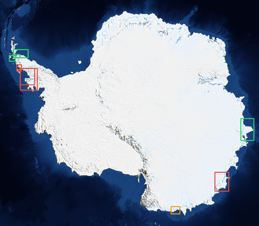
Figure 4: Spatial distribution of the scenes in the dataset. Scenes marked in green were used for model training, scenes marked in red were used for validation purposes. The red area in the top left is the “Antarctic Peninsula” validation site, while the bottom right red area is the “Wilkes Land” validation site. For most locations, data from 2 or 3 different sensing dates was used to allow for an assessment of each model’s temporal stability. Marked in yellow is the footprint of the visualization tile in Fig. 7.

Segmentation
SAR Gauss. Mixture [1] UNet [42] RDUNet [38] Gated-SCNN [44] HRNet+OCR [43] HED-UNet Ground Truth
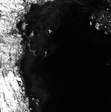
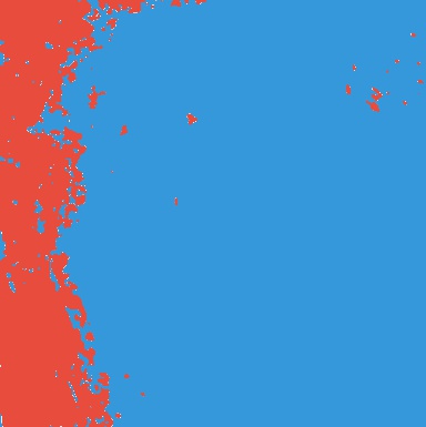
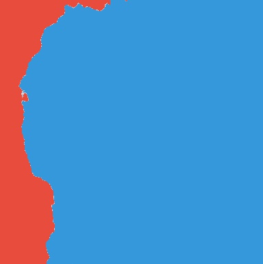
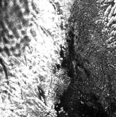
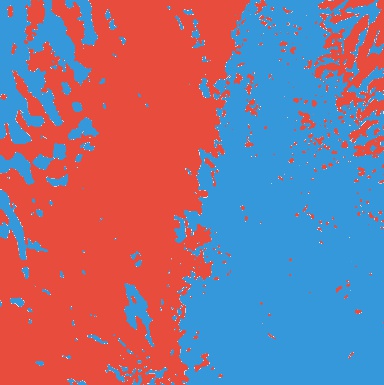
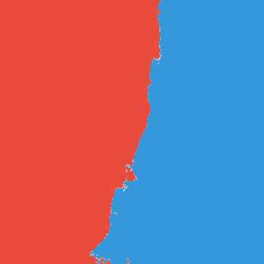
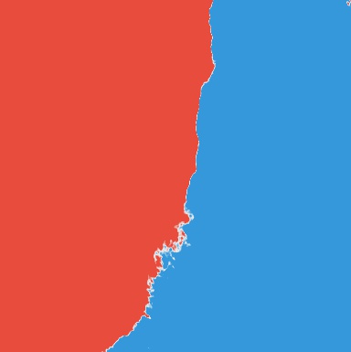
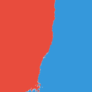
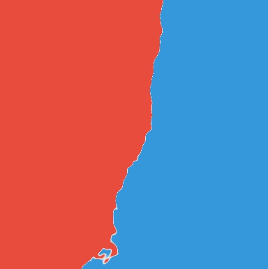
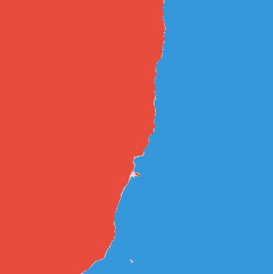
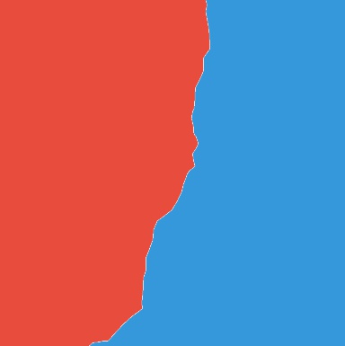
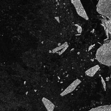
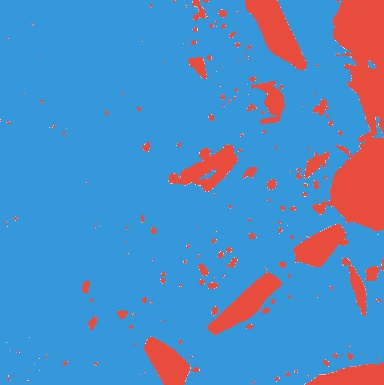
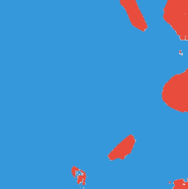
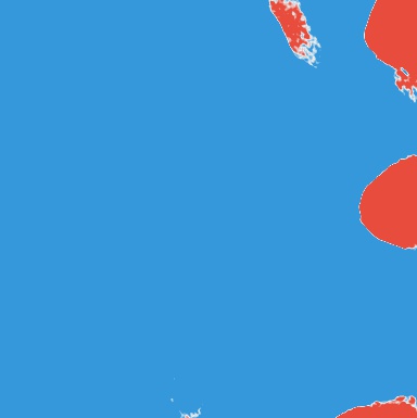
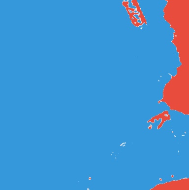
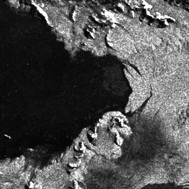
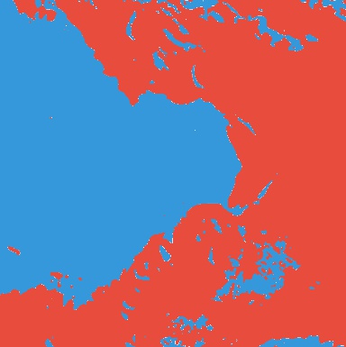
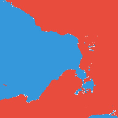
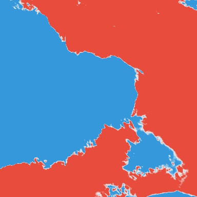
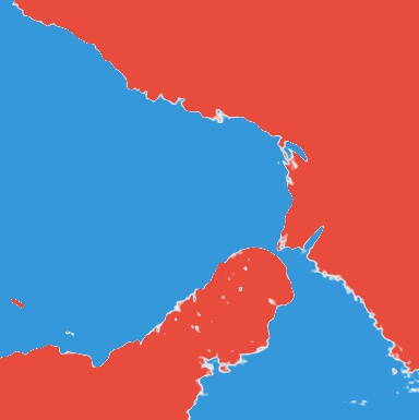
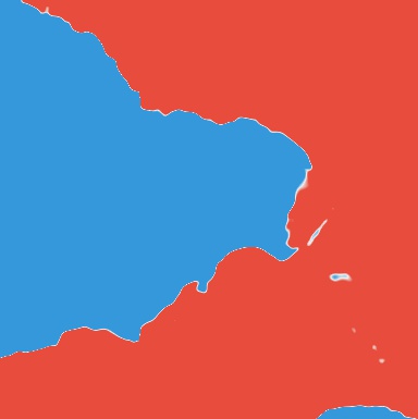
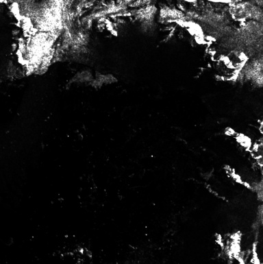
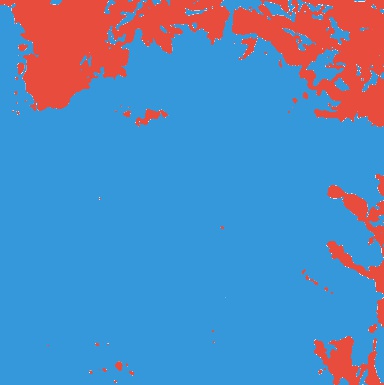
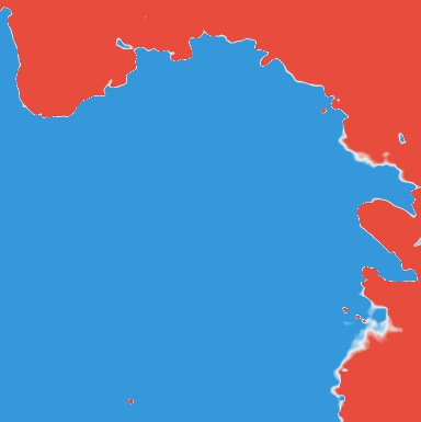
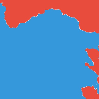
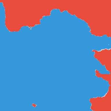
Edge Detection
SAR Active Contour [54] Sobel [47] HED [57] Gated-SCNN [44] HED-UNet Ground Truth

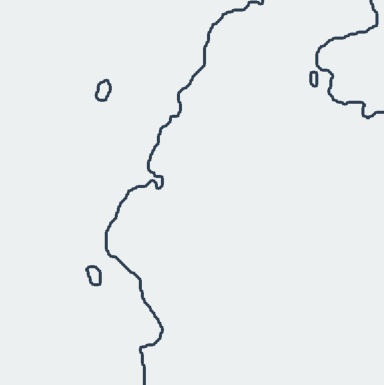
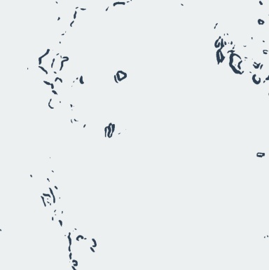
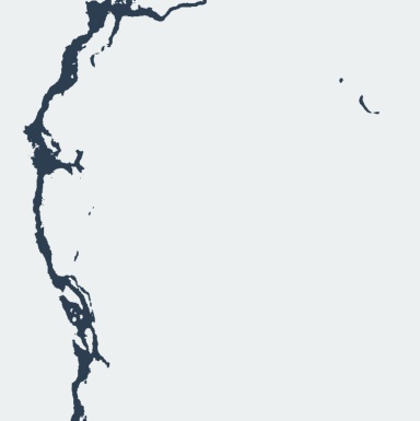
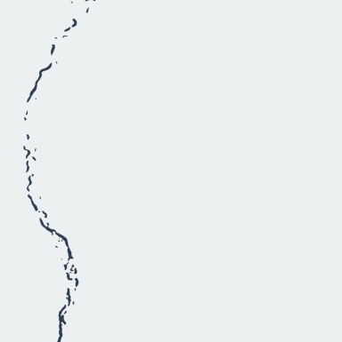
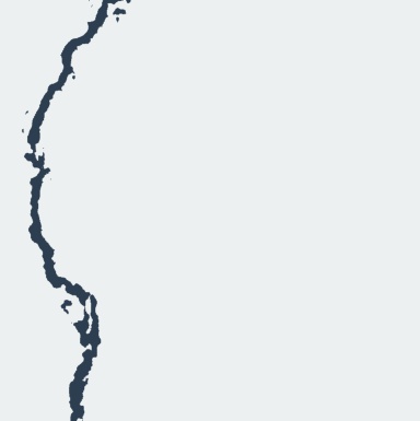
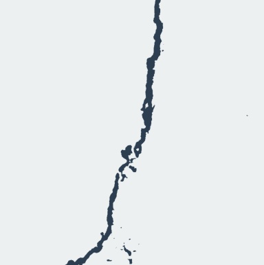
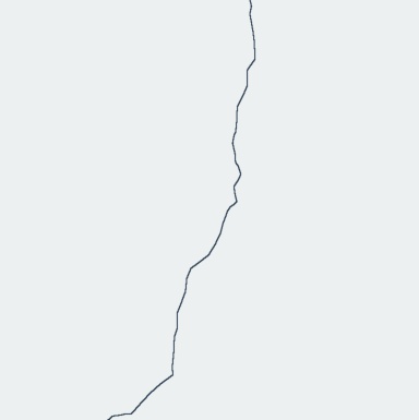
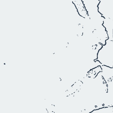
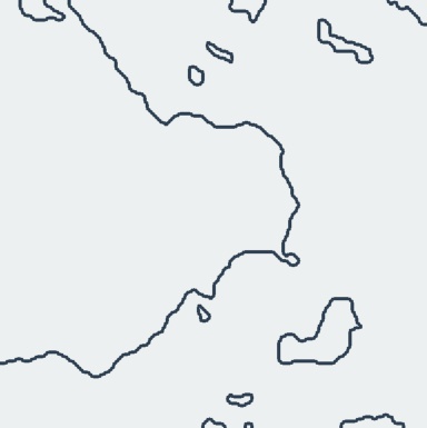
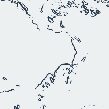
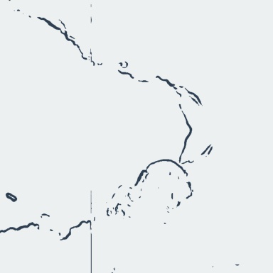
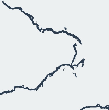
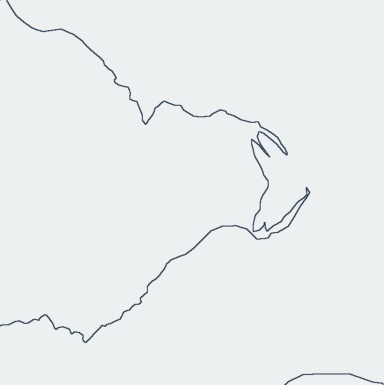
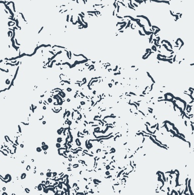
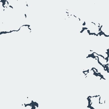
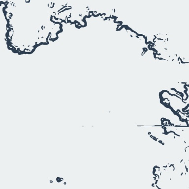
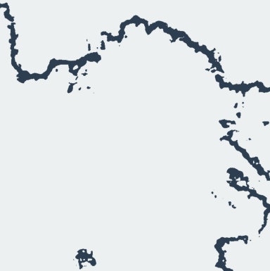
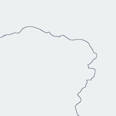
Figure 5: Qualitative results comparing the evaluated models on unseen validation tiles. In order to provide an informative visualization, the visualized tiles were selected to represent the full spectrum of easy (top) to hard (bottom) scenes within the validation set.

TABLE I: Numerical Results for the Evaluated Models

Site	Wilkes Land					Antarctic Peninsula
Metric	Accuracy	mIoU	Deviation	F1 ODS	F1 OIS	Accuracy	mIoU	Deviation	F1 ODS	F1 OIS
Gaussian Mixture [1]	77.4	63.0	773			74.7	58.8	765
K-Medians Clustering [36]	55.9	28.0	637			60.5	40.1	560
Sobel Edges [47]			507	29.0	31.8			644	21.1	20.8
Active Contours [54]			672	21.9	23.5			698	14.6	15.1
HED [57]			341$\,\pm\,$22	38.4$\,\pm\,$1.7	41.0$\,\pm\,$1.0			398$\,\pm\,$027	28.5$\,\pm\,$0.8	29.6$\,\pm\,$0.7
UNet [42]	89.2$\,\pm\,$3.0	80.6$\,\pm\,$4.7	271$\,\pm\,$14			79.3$\,\pm\,$2.8	65.0$\,\pm\,$4.4	483$\,\pm\,$040
DeepUNet [39]	87.3$\,\pm\,$6.4	77.6$\,\pm\,$9.9	287$\,\pm\,$32			76.9$\,\pm\,$4.8	61.8$\,\pm\,$7.5	525$\,\pm\,$118
RDUNet [38]	89.2$\,\pm\,$1.4	80.1$\,\pm\,$2.2	271$\,\pm\,$26			78.3$\,\pm\,$1.2	63.9$\,\pm\,$2.0	460$\,\pm\,$073
HRNet + OCR [43]	89.2$\,\pm\,$2.5	80.2$\,\pm\,$4.3	262$\,\pm\,$35			78.6$\,\pm\,$1.9	64.6$\,\pm\,$2.5	467$\,\pm\,$061
Gated-SCNN [44]	87.1$\,\pm\,$0.2	76.8$\,\pm\,$0.1	297$\,\pm\,$02	31.6$\,\pm\,$0.4	34.1$\,\pm\,$0.1	77.7$\,\pm\,$1.5	63.0$\,\pm\,$2.2	471$\,\pm\,$033	23.0$\,\pm\,$1.7	25.4$\,\pm\,$1.7
HED-UNet	92.0$\,\pm\,$0.8	84.9$\,\pm\,$1.4	222$\,\pm\,$23	39.7$\,\pm\,$1.2	41.6$\,\pm\,$0.9	80.5$\,\pm\,$1.6	67.2$\,\pm\,$2.2	345$\,\pm\,$024	27.1$\,\pm\,$1.9	29.4$\,\pm\,$1.8

In order to validate the effectiveness of the suggested improvements, we trained and validated several competing methods as well as the proposed model on a dataset of the Antarctic coast.

IV-A Dataset

Our dataset consists of 16 cropped Sentinel-1 GRD scenes of Antarctica’s coastline taken between June 2017 and December 2018 in the sensor’s Extra Wide Swath acquisition mode. The spatial distribution of these tiles can be seen in Fig. 4. The data has a resolution of 40 m and dual polarization with HH and HV channels. The cropped scenes have an average size of $7870\times 6572$ pixels ($$315\text{\,}\mathrm{km}$\times$263\text{\,}\mathrm{km}$$), and a combined area of around $730\,000\text{\,}\mathrm{k}\mathrm{m}^{2}$. All imagery is processed in the Antarctic Polar Stereographic projection (EPSG:3031) and converted to decibel. On these scenes, the coastline was manually annotated by experts in order to provide a ground truth sea-land segmentation and coastline delineation.

The scenes within the dataset are clustered in 4 areas, out of which 2 were selected as validation areas and completely left them out of the training procedure. This leads to a split of 11 training scenes and 5 validation scenes. The scenes were all tiled into sections of $768\times 768$ pixels with 50% overlap between adjacent tiles to form the training and validation dataset, respectively. In order to improve generalization performance, we employed 8-fold data augmentation on the training set. This augmentation technique processes a single tile into the 8 different versions that can be obtained by horizontal or vertical mirroring, as well as rotating by multiples of 90^∘.

IV-B Evaluated Models

As competitors to our model we evaluate the following models to provide a baseline.

IV-B1 Traditional Methods

Gaussian Mixture The sea-land segmentation method presented in [1], which applies dynamic thresholding based on a bimodal mixture of gaussians.
K-Medians Clustering An unsupervised sea-land segmentation method presented in [36] that employs k-medians clustering of the pixels in a scene on multiple scales.
Sobel Edges The coastline detection method presented in [47], which applies the Sobel filter, then a spatial dilution process, and then a Roberts edge filter.
Active Contours An active contours approach for coastline detection based on the Chan-Vese model [54].

IV-B2 Deep Learning

HED The edge detection model from [57].
UNet The segmentation model presented in [42], which is known to work well for coastline detection [31].
DeepUNet A modification of the previous method that was developed for sea-land segmentation as proposed in [39].
RDUNet Another modification of UNet developed for sea-land segmentation, which was proposed in [38].
HRNet + OCR One of the current state-of-the-art models for semantic segmentation in general computer vision [43].
Gated-SCNN Another recent model for semantic segmentation in general computer vision [44]. This one is particularly interesting, as it also combines segmentation with edge detection.

IV-C Training Details

The deep learning models were trained on the training dataset of Antarctic coastline scenes for 15 epochs on a Nvidia V100 card with 32GB of video memory. The model weights were optimized by an Adam optimizer using the hyperparameters suggested in [70], namely a learning rate of $0.001$, $\beta_{1}=0.9$, $\beta_{2}=0.999$ and $\varepsilon=10^{-8}$. Due to the large size of the used tiles, the batch size was set to the low number of 4 samples per batch.

V Results and Discussion

The improved performance from our method is quantified using the withheld validation dataset. To get informative insights on the actual coastline detection performance, the metrics are calculated only for pixels within $2\text{\,}\mathrm{km}$ of the true coastline. This way, a distortion of the metrics from non-coastal areas can be avoided.

The two validation areas (Antarctic Peninsula and Wilkes Land, see Fig. 4) are evaluated separately. While the Wilkes Land area can be considered of average difficulty, the Antarctic Peninsula seems to be a very tough location for all of the evaluated models.

For the segmentation approaches, we evaluate the pixelwise accuracy as well as the mean intersection-over-union metric for the classes of water and land. For edge detection, we calculate the edge $F_{1}$ scores at optimal image scale (OIS) and optimal dataset scale (ODS) Finally, we calculate an approximate deviation by averaging the distance to the ground truth coastline over all predicted coastline pixels (“Deviation”). Table I shows the numerical results obtained. The average distance metric can be considered the most important one for this task, as it estimates the overall error between the actual coastline and the predicted coastline. Regarding segmentation performance, the mIoU metric can be considered the primary metric. In order to get a visual impression of some of the models’ performance, Fig. 5 shows predictions for a selection of validation tiles. The shown examples are ordered from what we consider easy to hard samples for the models, and showcase some of the difficulties with the dataset, like sea ice and confounding backscatter on the higher ice sheet.

V-A Model Comparison

First, it is easy to see that the traditional models are not really competitive on this dataset. We ascribe this to the repeatedly stated phenomena of icebergs and ice sheet regions with difficult backscatter characteristics. As these models are unsupervised, they simply do not have a way of learning how to deal with such impediments.

Overall, the heterogeneity of the Antarctic coastline is astounding. While the coastline is found pretty well by most models in Wilkes Land, all models have trouble with the scenes from the Antarctic Peninsula.

Among the deep learning based models, UNet [42] imposes a respectable baseline, and even outperforms the more recent models like HRNet+OCR [43] and Gated-SCNN [44] in some of the evaluated metrics. Even though the latter also has a side output for edge detection, we find that its edge detection results fall short in comparison to HED [57] and HED-UNet. A reason for this might be the lack of a pretrained backbone network for Sentinel-1 data, which forced us to randomly initialize the backbone and train it alongside the rest of the network. Further, this model was optimized for segmentation of scenes with many different classes and small objects, which is needed for tasks like autonomous driving. In our usecase however, there are only two classes which are nearly equal in area, imposing a very different data distribution.

The ultimate goal of this study is to delineate the coastline as accurately as possible. In the corresponding average deviation metric, the proposed HED-UNet model outshines the alternative approaches, especially in the Antarctic Peninsula validation area. This confirms our assumptions that for this specific task, our considerations lead to increased performance.

V-B Network Depth and Deep Supervision

TABLE II: Numerical Results for the Ablations

Wilkes Land

Antarctic Peninsula

Data

Deep Sup.

Levels

Merging

Accuracy

mIoU

Deviation

F1 ODS

F1 OIS

Accuracy

mIoU

Deviation

F1 ODS

F1 OIS

SAR

Yes

5

Attention

90.3$\,\pm\,$1.3

82.2$\,\pm\,$2.1

239$\,\pm\,$16

37.2$\,\pm\,$0.7

38.7$\,\pm\,$0.9

77.0$\,\pm\,$1.0

62.5$\,\pm\,$1.3

379$\,\pm\,$45

25.4$\,\pm\,$1.2

27.0$\,\pm\,$1.0

SAR

No

6

Attention

88.5$\,\pm\,$1.4

79.2$\,\pm\,$2.3

954$\,\pm\,$07

7.1$\,\pm\,$0.5

7.1$\,\pm\,$0.5

80.3$\,\pm\,$1.6

66.8$\,\pm\,$2.1

895$\,\pm\,$07

7.4$\,\pm\,$0.2

7.5$\,\pm\,$0.2

SAR

Yes

6

None

89.7$\,\pm\,$1.2

81.1$\,\pm\,$1.9

284$\,\pm\,$37

37.5$\,\pm\,$1.2

39.7$\,\pm\,$1.3

81.8$\,\pm\,$2.0

69.0$\,\pm\,$2.9

378$\,\pm\,$35

28.0$\,\pm\,$1.8

30.2$\,\pm\,$1.8

SAR

Yes

6

Learned

89.9$\,\pm\,$2.5

81.6$\,\pm\,$3.9

236$\,\pm\,$14

37.0$\,\pm\,$2.2

38.6$\,\pm\,$2.2

81.4$\,\pm\,$1.1

68.3$\,\pm\,$1.6

391$\,\pm\,$12

26.6$\,\pm\,$1.4

29.1$\,\pm\,$1.4

SAR

Yes

6

Attention

92.0$\,\pm\,$0.8

84.9$\,\pm\,$1.4

222$\,\pm\,$23

39.7$\,\pm\,$1.2

41.6$\,\pm\,$0.9

80.5$\,\pm\,$1.6

67.2$\,\pm\,$2.2

345$\,\pm\,$24

27.1$\,\pm\,$1.9

29.4$\,\pm\,$1.8

SAR+DEM

Yes

6

Attention

92.9$\,\pm\,$1.4

86.7$\,\pm\,$2.4

226$\,\pm\,$47

35.1$\,\pm\,$3.4

36.0$\,\pm\,$3.5

91.6$\,\pm\,$1.6

84.6$\,\pm\,$2.7

210$\,\pm\,$09

30.7$\,\pm\,$2.1

31.4$\,\pm\,$2.7

As a means of quantifying the improvements made to the architecture, we evaluate versions of our model with only some of the improvements applied. The results of this ablation study are displayed in Table II.

For a fair comparison with UNet-based models, we evaluate the performance when only 5 resolution levels are used instead of 6, corresponding to 4 down- and upsampling steps instead of 5. While this setup performs slightly worse than the full HED-UNet, it still outperforms the baseline methods.

Regarding deep supervision, we can see that it is of paramount importance for edge detection performance. Without it, the model is barely able to predict the presence of edges. What is more, the coastline is often missed completely due to this poor edge detection performance. On the other hand, deep supervision does not seem to alter the performance on the semantic segmentation task much. This is in line with the original models that we took inspiration from. While the segmentation model UNet [42] does not employ deep supervision, the edge detection model HED [57] makes heavy use of it.

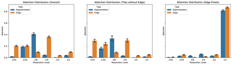
Figure 6: Amount of attention spent on the different resolution levels. Each plot analyzes a specific class of pixels in the validation dataset – from left to right: Average over all pixels, average over pixels from edge-less tiles, average over all edge pixels.

V-C Merging Strategies

After adding the deep supervision, we evaluate different merging strategies:

None

First, we evaluate a configuration where just the last layer of the decoder is used for the predictions (denoted “None”). This corresponds to the workings of a UNet [42] model with two final prediction layers, one for each task.

Learned

Secondly, we evaluate the performance of the learned merging strategy, as originally proposed in [57]. Here, a prediction is computed for each resolution level in the feature pyramid. These predictions are then upsampled to full resolution and concatenated. After this, a 1$\times$1 convolutional layer with learned weights computes the final prediction from the concatenated prediction stack.

Attention

The last strategy is the hierarchical attention merging introduced in Sect. III-C, which ]newdoes not rely on fixed weights like the previous strategy, but computes the merging weights dynamically for each pixel within each scene.
From our results, learned merging does not improve much over no merging for segmentation, and even performs a bit worse for edge detection. The average deviation improves quite a bit in Wilkes Land, but worsens a bit on the Antarctic Peninsula in return. We ascribe this to the large differences in the validation areas. As the merging coefficients are fixed for the “Learned” approach, this might hint at the fact that the model learns coefficients that work well for Wilkes Land, but less so for the Antarctic Peninsula.

This issue is overcome by our newly proposed attention merging strategy, which can adapt to the different scenes. It can learn to find good sets of merging coefficients for both Wilkes Land and the Antarctic Peninsula, even though the optimal values for each one might be different.

Fig. 6 shows that the model indeed directs its attention in an adaptive fashion as we conjectured. Overall, a mix of all resolution levels is used to compute the final output. On tiles that are completely covered by one of the two classes, the attention shifts a bit towards the lower resolution levels, as they tend to provide more robust predictions. For pixels on the edge, the model heavily focuses on the highest available resolution level, in order to arrive at accurate delineations in these regions.

Figure 7: A section of George V Coast with Cape Hudson in the bottom left, imagery mosaiced from Sentinel-1 takes in early 2019. This scene is both temporally and spatially separated from the training and validation sets used. Overlaid in red is the coastline predicted by the HED-UNet model.

SAR/DEM	HED-UNet	Ground Truth

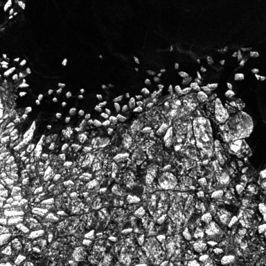
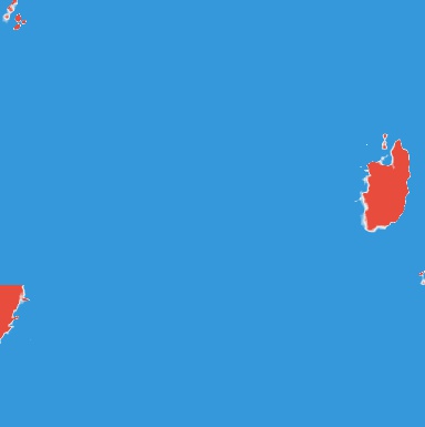
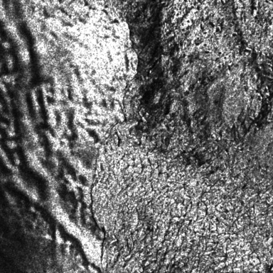
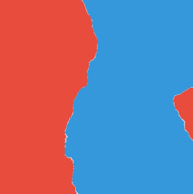
Figure 8: Failure modes of the proposed model. Top: Confusion from a very large cluster of sea ice. Bottom: Confusion due to missing context at the border of the tile

V-D DEM Experiments

Further, we look into including digital elevation data from the TanDEM-X elevation model [71]. We conjecture that this secondary data source can help the model better deject misclassifications from icebergs or dry-snow facies of the higher ice sheet, which have confounding SAR backscatter.

To discourage the model from directly reproducing the coastline implied by the elevation model, we decided to downsample the DEM’s resolution to $640\text{\,}\mathrm{m}$. This resolution is coarse enough to not make a segmentation based on the DEM alone competitive to the non-DEM models, which have an average deviation of less than $300\text{\,}\mathrm{m}$. Further, it allows for easy feature fusion, as it corresponds to the resolution of the feature map at $\nicefrac{{1}}{{16}}$ of the full resolution. Therefore, it is simply concatenated to the feature map after the fourth downsampling step in the encoder.

The results when including the DEM are displayed as the last ablation in Table II. On the very hard scenes of the Arctic Peninsula, this additional information helps the model by a large margin, boosting the average deviation from $345\text{\,}\mathrm{m}$ to $210\text{\,}\mathrm{m}$. However, the story is different for Wilkes Land. Here, the deviation worsens slightly, and the edge detection metrics go down considerably.

This is a strong indicator that the model is indeed overfitting on the DEM to some extent. For example, in some highly dynamic coastal regions the model will be confused when the DEM and SAR imagery are contradictory.

So all in all the inclusion of DEM data can be beneficial, but needs to be done very carefully to prevent the model from overfitting to the DEM alone.

V-E Limitations

Even though the newly proposed model outperforms the baselines on nearly all validation scenes, there are still cases where the results are not perfect. Most misclassifications can be attributed to one of two failure modes, which we will now briefly discuss. Visual examples for these failure modes can be seen in Fig. 8.

V-E1 Sea Ice

The large receptive field and multitask training help alleviate the issue of wrongly classified sea ice. But very large icebergs and areas of ice mélange can still throw off the proposed model. The first failure example displays such an area where large clusters of sea ice confuse the model.

V-E2 Missing Context

For areas close to the border of a tile, the model sometimes does not have enough contextual information to correctly classify them. This can be observed in the second failure visualization, where a patch of sea ice directly next to the tile border is wrongly classified as land.

Overall, these failures do not occur often throughout the dataset and apply not only to the HED-UNet models, but to the other compared models as well. Especially the first one requires much human interpretation on a large spatial context, which is difficult for a neural network to achieve without general reasoning capabilities.

V-F Effective Receptive Fields

Deep CNNs like the ones used in our experiments have very large theoretical receptive fields. It is conjectured that while long-range connections are theoretically possible in these networks, networks will often ignore them in favor of short-range connections.

UNet [42]	Gated-SCNN [44]
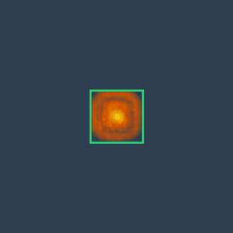
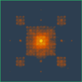
HRNet+OCR [43]	HED-UNet

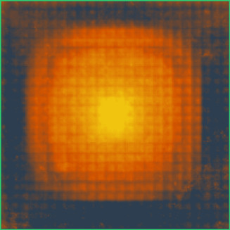
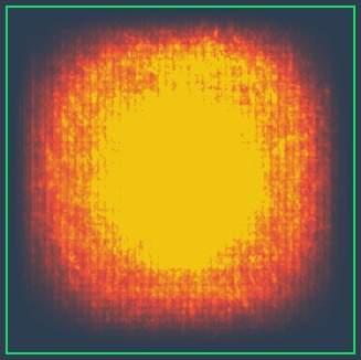
Figure 9: Effective receptive fields of some tested models for the prediction of a central pixel, visualized in image space. Theoretical receptive fields outlined in green. Note that the theoretical receptive fields of Gated-SCNN and HRNet+OCR are larger than the used patch size of 768$\times$768.

To assess how much of the spatial context is actually used by a CNN, its so-called effective receptive field (ERF) can be estimated [72]. This is done by analyzing the expected gradient magnitude of each input pixel with respect to a central output pixel. For a CNN $f$ and a sequence of input images $I_{k}$, one therefore looks at the values of

$$E=\frac{1}{n}\sum_{k=1}^{n}\left|\nabla_{I_{k}}f(I_{k})_{i,j}\right|$$ (5)

for a central output pixel $(i,j)$. If for an input pixel $(x,y)$, the value $E_{x,y}$ is non-negligible, then this pixel will influence the output predictions at position $(i,j)$. The spatial distribution of these relevant pixels is then called the effective receptive field.

As the gradient magnitude gives insight on how much the prediction changes in response to a change in the input, the ERF allows for a measurement of the spatial context used by the model. A model with a larger ERF bases its decisions on a larger spatial context than one with a small ERF.

We conjectured that for the task of Antarctic coastline detection, a model needs to take a large context window into account. And indeed, there seems to be a correlation between a larger ERF and better validation scores for this task.

It can be observed that the UNet model is limited by its theoretical receptive field. Its ERF is forced into an almost quadratic shape because of this. The ERF of the Gated-SCNN model is particularly interesting with it’s fractal-like shape. We conjecture that this is due to the Atrous Spatial Pyramid Pooling block used in the network architecture, which makes heavy use of dilated convolutions.

Finally, the HRNet+OCR and HED-UNet models employ a very large ERF, which once more supports our assumption that a large receptive field is needed for coastline detection in Antarctica.

VI Conclusion

In this paper, we introduced a model for simultaneous segmentation and edge detection. The proposed HED-UNet learns to exploit the synergies between the two tasks, and thereby manages to surpass both edge detection and semantic segmentation baselines. By the use of deep supervision, we encourage the model to encode meaningful features in its deep layers, which allow for more general predictions. Finally, the proposed attention merging heads allow for better learning performance and more robust classifications.

Compared to approaching the task with a regular UNet, the presented network architecture only requires little additional computational cost. Most of the performance gains stem from the adapted training procedure and a few additional layers, which do not require many computational resources compared to the layers already present.

While it is not a general purpose model, we show that our proposed improvements to the model are indeed beneficial for the task of coastline detection. Visual and numerical inspection of the results confirm our assumption that the combination of the two tasks helps the model better grasp the concept of a coastline.

Our model can be applied to coastline detection tasks not only in polar regions, but to coastal regions worldwide. Further, we are convinced that the approach taken by HED-UNet will greatly benefit other tasks requiring an edge detection approach in combination with semantic segmentation. Possible applications include the mapping of building footprints, roads, and bodies of water like lakes or rivers.

References

- [1] H. Liu and K. C. Jezek, “A complete high-resolution coastline of Antarctica extracted from orthorectified Radarsat SAR Imagery,” Photogramm. Eng. Remote Sens., vol. 70, no. 5, pp. 605–616, May 2004.
- [2] J. Geng, H. Wang, J. Fan, and X. Ma, “Deep supervised and contractive neural network for SAR image classification,” IEEE Trans. Geosci. Remote Sens., vol. 55, no. 4, pp. 2442–2459, Apr. 2017.
- [3] C. Robinson, L. Hou, K. Malkin, R. Soobitsky, J. Czawlytko, B. Dilkina, and N. Jojic, “Large scale high-resolution land cover mapping with multi-resolution data,” Proc. 2019 IEEE Conf. Comput. Vis. Pattern Recognit. (CVPR), pp. 12 726–12 735, 2019.
- [4] X.-Y. Tong, G.-S. Xia, Q. Lu, H. Shen, S. Li, S. You, and L. Zhang, “Land-cover classification with high-resolution remote sensing images using transferable deep models,” Remote Sens. Environ., vol. 237, p. 111322, Feb. 2020.
- [5] F. Eugenio, J. Marcello, and J. Martin, “High-resolution maps of bathymetry and benthic habitats in shallow-water environments using multispectral remote sensing imagery,” IEEE Trans. Geosci. Remote Sens., vol. 53, no. 7, pp. 3539–3549, Jul. 2015.
- [6] J. Liang, J. Zhang, Y. Ma, and C.-Y. Zhang, “Derivation of bathymetry from high-resolution optical satellite imagery and USV sounding data,” Mar. Geod., vol. 40, no. 6, pp. 466–479, Nov. 2017.
- [7] M. Erena, J. A. Domínguez, J. F. Atenza, S. García-Galiano, J. Soria, and Á. Pérez-Ruzafa, “Bathymetry time series using high spatial resolution satellite images,” Water, vol. 12, no. 2, p. 531, Feb. 2020.
- [8] Y. Long, Y. Gong, Z. Xiao, and Q. Liu, “Accurate object localization in remote sensing images based on convolutional neural networks,” IEEE Trans. Geosci. Remote Sens., vol. 55, no. 5, pp. 2486–2498, May 2017.
- [9] N. Audebert, B. Le Saux, and S. Lefèvre, “Beyond RGB: Very high resolution urban remote sensing with multimodal deep networks,” ISPRS J. Photogramm. Remote Sens., vol. 140, pp. 20–32, Jun. 2018.
- [10] L. Mou and X. X. Zhu, “Vehicle instance segmentation from aerial image and video using a multitask learning residual fully convolutional network,” IEEE Trans. Geosci. Remote Sens., vol. 56, no. 11, pp. 6699–6711, Nov. 2018.
- [11] L. Mou, Y. Hua, and X. X. Zhu, “Relation matters: Relational context-aware fully convolutional network for semantic segmentation of high-resolution aerial images,” IEEE Trans. Geosci. Remote Sens., pp. 1–13, 2020.
- [12] Q. Li, Y. Shi, X. Huang, and X. X. Zhu, “Building footprint generation by integrating convolution neural network with feature pairwise conditional random field (FPCRF),” IEEE Trans. Geosci. Remote Sens., pp. 1–18, 2020.
- [13] D. Wen, X. Huang, L. Zhang, and J. A. Benediktsson, “A novel automatic change detection method for urban high-resolution remotely sensed imagery based on multiindex scene representation,” IEEE Trans. Geosci. Remote Sens., vol. 54, no. 1, pp. 609–625, Jan. 2016.
- [14] O. A. Ajadi, F. J. Meyer, and P. W. Webley, “Change detection in synthetic aperture radar images using a multiscale-driven approach,” Remote Sens., vol. 8, no. 6, p. 482, Jun. 2016.
- [15] Z. Y. Lv, T. F. Liu, P. Zhang, J. A. Benediktsson, T. Lei, and X. Zhang, “Novel adaptive histogram trend similarity approach for land cover change detection by using bitemporal very-high-resolution remote sensing images,” IEEE Trans. Geosci. Remote Sens., vol. 57, no. 12, pp. 9554–9574, Dec. 2019.
- [16] B. Du, L. Ru, C. Wu, and L. Zhang, “Unsupervised deep slow feature analysis for change detection in multi-temporal remote sensing images,” IEEE Trans. Geosci. Remote Sens., vol. 57, no. 12, pp. 9976–9992, Dec. 2019.
- [17] C. Zhang, S. Wei, S. Ji, and M. Lu, “Detecting large-scale urban land cover changes from very high resolution remote sensing images using cnn-based classification,” ISPRS Int. J. Geo-Inf., vol. 8, no. 4, p. 189, Apr. 2019.
- [18] M. Engram, C. D. Arp, B. M. Jones, O. A. Ajadi, and F. J. Meyer, “Analyzing floating and bedfast lake ice regimes across Arctic Alaska using 25 years of space-borne SAR imagery,” Remote Sens. Environ., vol. 209, pp. 660–676, May 2018.
- [19] I. Sasgen, H. Konrad, V. Helm, and K. Grosfeld, “High-resolution mass trends of the Antarctic ice sheet through a spectral combination of satellite gravimetry and radar altimetry observations,” Remote Sens., vol. 11, no. 2, p. 144, Jan. 2019.
- [20] D. O. Dammann, L. E. B. Eriksson, A. R. Mahoney, H. Eicken, and F. J. Meyer, “Mapping pan-Arctic landfast sea ice stability using Sentinel-1 interferometry,” The Cryosphere, vol. 13, no. 2, pp. 557–577, Feb. 2019.
- [21] I. Nitze, G. Grosse, B. M. Jones, V. E. Romanovsky, and J. Boike, “Remote sensing quantifies widespread abundance of permafrost region disturbances across the Arctic and Subarctic,” Nat. Commun., vol. 9, no. 1, pp. 1–11, Dec. 2018.
- [22] J. E. Anderson, T. A. Douglas, R. A. Barbato, S. Saari, J. D. Edwards, and R. M. Jones, “Linking vegetation cover and seasonal thaw depths in interior Alaska permafrost terrains using remote sensing,” Remote Sens. Environ., vol. 233, p. 111363, Nov. 2019.
- [23] C. A. Baumhoer, A. J. Dietz, S. Dech, and C. Kuenzer, “Remote sensing of Antarctic glacier and ice-shelf front dynamics—A review,” Remote Sens., vol. 10, no. 9, p. 1445, Sep. 2018.
- [24] T. Strozzi, A. Luckman, T. Murray, U. Wegmuller, and C. Werner, “Glacier motion estimation using SAR offset-tracking procedures,” IEEE Trans. Geosci. Remote Sens., vol. 40, no. 11, pp. 2384–2391, Nov. 2002.
- [25] G. Vasile, E. Trouve, I. Petillot, P. Bolon, J.-M. Nicolas, M. Gay, J. Chanussot, T. Landes, P. Grussenmeyer, V. Buzuloiu, I. Hajnsek, C. Andres, M. Keller, and R. Horn, “High-resolution SAR interferometry: Estimation of local frequencies in the context of Alpine glaciers,” IEEE Trans. Geosci. Remote Sens., vol. 46, no. 4, pp. 1079–1090, Apr. 2008.
- [26] E. Erten, “Glacier velocity estimation by means of a polarimetric similarity measure,” IEEE Trans. Geosci. Remote Sens., vol. 51, no. 6, pp. 3319–3327, Jun. 2013.
- [27] V. Akbari, A. P. Doulgeris, and T. Eltoft, “Monitoring glacier changes using multitemporal multipolarization SAR images,” IEEE Trans. Geosci. Remote Sens., vol. 52, no. 6, pp. 3729–3741, Jun. 2014.
- [28] S. Lang, X. Liu, B. Zhao, X. Chen, and G. Fang, “Focused synthetic aperture radar processing of ice-sounding data collected over the east antarctic ice sheet via the modified range migration algorithm using curvelets,” IEEE Trans. Geosci. Remote Sens., vol. 53, no. 8, pp. 4496–4509, Aug. 2015.
- [29] L. Krieger and D. Floricioiu, “Automatic calving front delineation on TerraSAR-X and Sentinel-1 SAR imagery,” in Proc. 2017 IEEE Int. Geosci. Remote Sens. Symp. (IGARSS), Jul. 2017, pp. 2817–2820.
- [30] V. Akbari and C. Brekke, “Iceberg detection in open and ice-infested waters using C-band polarimetric synthetic aperture radar,” IEEE Trans. Geosci. Remote Sens., vol. 56, no. 1, pp. 407–421, Jan. 2018.
- [31] C. A. Baumhoer, A. J. Dietz, C. Kneisel, and C. Kuenzer, “Automated extraction of antarctic glacier and ice shelf fronts from sentinel-1 imagery using deep learning,” Remote Sens., vol. 11, no. 21, p. 2529, Jan. 2019.
- [32] E. Zhang, L. Liu, and L. Huang, “Automatically delineating the calving front of Jakobshavn Isbræ from multitemporal TerraSAR-X images: A deep learning approach,” The Cryosphere, vol. 13, no. 6, pp. 1729–1741, Jun. 2019.
- [33] Y. Mohajerani, M. Wood, I. Velicogna, and E. Rignot, “Detection of glacier calving margins with convolutional neural networks: A case study,” Remote Sens., vol. 11, no. 1, p. 74, Jan. 2019.
- [34] B. W. J. Miles, C. R. Stokes, and S. S. R. Jamieson, “Simultaneous disintegration of outlet glaciers in Porpoise Bay (Wilkes Land), East Antarctica, driven by sea ice break-up,” The Cryosphere, vol. 11, no. 1, pp. 427–442, Feb. 2017.
- [35] Y. Liu, J. C. Moore, X. Cheng, R. M. Gladstone, J. N. Bassis, H. Liu, J. Wen, and F. Hui, “Ocean-driven thinning enhances iceberg calving and retreat of Antarctic ice shelves,” Proc. Natl. Acad. Sci., vol. 112, no. 11, pp. 3263–3268, Mar. 2015.
- [36] M. Schmitt, G. Baier, and X. X. Zhu, “Potential of nonlocally filtered pursuit monostatic TanDEM-X data for coastline detection,” ISPRS J. Photogramm. Remote Sens., vol. 148, pp. 130–141, Feb. 2019.
- [37] X. X. Zhu, D. Tuia, L. Mou, G. Xia, L. Zhang, F. Xu, and F. Fraundorfer, “Deep learning in remote sensing: A comprehensive review and list of resources,” IEEE Geosci. Remote Sens. Mag., vol. 5, no. 4, pp. 8–36, 2017.
- [38] P. Shamsolmoali, M. Zareapoor, R. Wang, H. Zhou, and J. Yang, “A novel deep structure U-Net for sea-land segmentation in remote sensing images,” IEEE J. Sel. Top. Appl. Earth Obs. Remote Sens., vol. 12, no. 9, pp. 3219–3232, Sep. 2019.
- [39] R. Li, W. Liu, L. Yang, S. Sun, W. Hu, F. Zhang, and W. Li, “DeepUNet: A deep fully convolutional network for pixel-level sea-land segmentation,” IEEE J. Sel. Top. Appl. Earth Obs. Remote Sens., vol. 11, no. 11, pp. 3954–3962, Nov. 2018.
- [40] Z. Chu, T. Tian, R. Feng, and L. Wang, “Sea-land segmentation with Res-UNet and fully connected CRF,” in Proc. 2019 IEEE Int. Geosci. Remote Sens. Symp. (IGARSS), Jul. 2019, pp. 3840–3843.
- [41] V. Badrinarayanan, A. Kendall, and R. Cipolla, “SegNet: A deep convolutional encoder-decoder architecture for image segmentation,” IEEE Trans. Pattern Anal. Mach. Intell., vol. 39, no. 12, pp. 2481–2495, Dec. 2017.
- [42] O. Ronneberger, P. Fischer, and T. Brox, “U-Net: Convolutional networks for biomedical image segmentation,” in Proc. Int. Conf. Med. Image Comput. Comput.-Assist. Intervent. (MICCAI), N. Navab, J. Hornegger, W. M. Wells, and A. F. Frangi, Eds., Oct. 2015, pp. 234–241.
- [43] Y. Yuan, X. Chen, and J. Wang, “Object-contextual representations for semantic segmentation,” in Computer Vision - ECCV 2020, A. Vedaldi, H. Bischof, T. Brox, and J.-M. Frahm, Eds. Cham: Springer International Publishing, 2020, pp. 173–190.
- [44] T. Takikawa, D. Acuna, V. Jampani, and S. Fidler, “Gated-scnn: Gated shape CNNs for semantic segmentation,” Proc. IEEE CVF Int. Conf. Comput. Vis. ICCV, Oct. 2019.
- [45] L. G. Roberts, “Machine perception of three-dimensional solids,” Ph.D. dissertation, Massachusetts Institute of Technology, 1963.
- [46] W. K. Pratt, “Edge detection,” in Digital Image Processing. John Wiley & Sons, Ltd, 2006, pp. 465–533.
- [47] J.-S. Lee and I. Jurkevich, “Coastline detection and tracing In SAR images,” IEEE Trans. Geosci. Remote Sens., vol. 28, no. 4, pp. 662–668, Jul. 1990.
- [48] D. Wang and X. Liu, “Coastline extraction from SAR images using robust ridge tracing,” Marine Geodesy, vol. 42, no. 3, pp. 286–315, May 2019.
- [49] M. Modava, G. Akbarizadeh, and M. Soroosh, “Integration of spectral histogram and level set for coastline detection in SAR images,” IEEE Trans. Aerosp. Electron. Syst., vol. 55, no. 2, pp. 810–819, Apr. 2019.
- [50] M. Kass, A. Witkin, and D. Terzopoulos, “Snakes: Active contour models,” Int. J. Comput. Vis., vol. 1, no. 4, pp. 321–331, Jan. 1988.
- [51] T. Klinger, M. Ziems, C. Heipke, H. W. Schenke, and N. Ott, “Antarctic Coastline Detection using Snakes,” Photogramm. - Fernerkund. - Geoinformation, vol. 2011, no. 6, pp. 421–434, Dec. 2011.
- [52] C. Liu, Y. Xiao, and J. Yang, “A coastline detection method in polarimetric SAR images mixing the region-based and edge-based active contour models,” IEEE Trans. Geosci. Remote Sens., vol. 55, no. 7, pp. 3735–3747, Jul. 2017.
- [53] S. Osher and J. A. Sethian, “Fronts propagating with curvature-dependent speed: Algorithms based on Hamilton-Jacobi formulations,” Journal of Computational Physics, vol. 79, no. 1, pp. 12–49, Nov. 1988.
- [54] T. Chan and L. Vese, “An active contour model without edges,” in Scale-Space Theories in Computer Vision. Springer, Berlin, Heidelberg, Sep. 1999, pp. 141–151.
- [55] C. Liu, J. Yang, J. Yin, and W. An, “Coastline detection in SAR images using a hierarchical level set segmentation,” IEEE J. Sel. Top. Appl. Earth Obs. Remote Sens., vol. 9, no. 11, pp. 4908–4920, Nov. 2016.
- [56] M. Modava and G. Akbarizadeh, “A level set based method for coastline detection of SAR images,” in 3rd International Conference on Pattern Recognition and Image Analysis (IPRIA). Shahrekord, Iran: IEEE, Apr. 2017, pp. 253–257.
- [57] S. Xie and Z. Tu, “Holistically-nested edge detection,” in IEEE Int. Conf. Comput. Vis. (ICCV), Dec. 2015, pp. 1395–1403.
- [58] Y. Liu, M.-M. Cheng, X. Hu, K. Wang, and X. Bai, “Richer convolutional features for edge detection,” Proc. 2017 IEEE Conf. Comput. Vis. Pattern Recognit. CVPR, Jul. 2017.
- [59] X. S. Poma, E. Riba, and A. Sappa, “Dense extreme inception network: Towards a robust CNN model for edge detection,” Proc. IEEE CVF Winter Conf. Appl. Comput. Vis. WACV, Mar. 2020.
- [60] D. Cheng, G. Meng, G. Cheng, and C. Pan, “SeNet: Structured edge network for sea–land segmentation,” IEEE Geosci. Remote Sens. Lett., vol. 14, no. 2, p. 5, 2017.
- [61] Z. Jiang, Z. Chen, K. Ji, and J. Yang, “Semantic segmentation network combined with edge detection for building extraction in remote sensing images,” in Int. Symp. Multispect. Image Processing Pattern Recognit. (MIPPR), vol. 11430. International Society for Optics and Photonics, Feb. 2020, p. 114300D.
- [62] D. Cheng, G. Meng, S. Xiang, and C. Pan, “FusionNet: Edge aware deep convolutional networks for semantic segmentation of remote sensing harbor images,” IEEE J. Sel. Top. Appl. Earth Obs. Remote Sens., vol. 10, no. 12, pp. 5769–5783, Dec. 2017.
- [63] L.-C. Chen, J. T. Barron, G. Papandreou, K. Murphy, and A. L. Yuille, “Semantic image segmentation with task-specific edge detection using cnns and a discriminatively trained domain transform,” Proc. 2016 IEEE Conf. Comput. Vis. Pattern Recognit. (CVPR), pp. 4545–4554, Jun. 2016.
- [64] D. Marmanis, K. Schindler, J. D. Wegner, S. Galliani, M. Datcu, and U. Stilla, “Classification with an edge: Improving semantic image segmentation with boundary detection,” ISPRS J. Photogramm. Remote Sens., vol. 135, pp. 158–172, Jan. 2018.
- [65] L.-C. Chen, G. Papandreou, F. Schroff, and H. Adam, “Rethinking atrous convolution for semantic image segmentation,” ArXiv170605587 Cs, Dec. 2017.
- [66] T. Lin, P. Dollár, R. Girshick, K. He, B. Hariharan, and S. Belongie, “Feature pyramid networks for object detection,” Proc. 2017 IEEE Conf. Comput. Vis. Pattern Recognit. CVPR, pp. 936–944, 2017.
- [67] C.-Y. Lee, S. Xie, P. Gallagher, Z. Zhang, and Z. Tu, “Deeply-supervised nets,” in Int. Conf. Artif. Intell. Stat. (AISTATS), G. Lebanon and S. V. N. Vishwanathan, Eds., vol. 38, May 2015, pp. 562–570.
- [68] A. Vaswani, N. Shazeer, N. Parmar, J. Uszkoreit, L. Jones, A. N. Gomez, Ł. Kaiser, and I. Polosukhin, “Attention is all you need,” Adv. Neural Inf. Process. Syst., vol. 30, p. 11, 2017.
- [69] X. Wang, R. Girshick, A. Gupta, and K. He, “Non-local neural networks,” Proc. 2018 IEEE Conf. Comput. Vis. Pattern Recognit. (CVPR), pp. 7794–7803, 2018.
- [70] D. P. Kingma and J. Ba, “Adam: A method for stochastic optimization,” 3rd Int. Conf. Learn. Represent. ICLR, 2015.
- [71] P. Rizzoli, M. Martone, C. Gonzalez, C. Wecklich, D. Borla Tridon, B. Bräutigam, M. Bachmann, D. Schulze, T. Fritz, M. Huber, B. Wessel, G. Krieger, M. Zink, and A. Moreira, “Generation and performance assessment of the global TanDEM-X digital elevation model,” ISPRS J. Photogramm. Remote Sens., vol. 132, pp. 119–139, Oct. 2017.
- [72] W. Luo, Y. Li, R. Urtasun, and R. Zemel, “Understanding the effective receptive field in deep convolutional neural networks,” in Int. Conf. Neural Inf. Process. Syst. (NIPS), Dec. 2016, pp. 4905–4913.