The KL-Divergence between a Graph Model and its Fair I-Projection as a Fairness Regularizer

Abstract

Learning and reasoning over graphs is increasingly done by means of probabilistic models, e.g. exponential random graph models, graph embedding models, and graph neural networks. When graphs are modeling relations between people, however, they will inevitably reflect biases, prejudices, and other forms of inequity and inequality. An important challenge is thus to design accurate graph modeling approaches while guaranteeing fairness according to the specific notion of fairness that the problem requires. Yet, past work on the topic remains scarce, is limited to debiasing specific graph modeling methods, and often aims to ensure fairness in an indirect manner.

We propose a generic approach applicable to most probabilistic graph modeling approaches. Specifically, we first define the class of fair graph models corresponding to a chosen set of fairness criteria. Given this, we propose a fairness regularizer defined as the KL-divergence between the graph model and its I-projection onto the set of fair models. We demonstrate that using this fairness regularizer in combination with existing graph modeling approaches efficiently trades-off fairness with accuracy, whereas the state-of-the-art models can only make this trade-off for the fairness criterion that they were specifically designed for.

1 Introduction

Graphs are flexible data structures, naturally suited for representing relations between people (e.g. in social networks) or between people and objects (e.g. in recommender systems). Here, links between nodes may represent any kind of relation, such as interest or similarity. It is common in real-world relational data that the corresponding graphs are often imperfect or only partially observed. For example, it may contain spurious or missing edges, or some node pairs may be explicitly marked as having unknown status. In such cases, it is often useful to correct or predict the link status between any given pair of nodes. This task is known as link prediction: predicting the link status between any pair of nodes, given the known part of the graph and possibly any node or edge features [23].

Methods for link prediction are typically based on machine learning. A first class of methods constructs a set of features for each node-pair, such as their number of common neighbors, the Jaccard similarity between their neighborhoods, and more [24]. Other methods are based on probabilistic models, with exponential random graph models as a notable class originating mostly from the statistics and physics communities [30]. More recently, the machine learning community has proposed graph embedding methods [14], which represent each node as a point in a vector space, from which a probabilistic model for the graph’s edges can be derived (among other possible uses). Related to this, graph neural network models [33] have been proposed which equally can be used to probabilistically model the presence or absence of edges in a graph [35].

The use of such models can have genuine impact on the lives of the individuals concerned. For example, a graph of data on job seekers and job vacancies can be used to determine which career opportunities an individual will be recommended. If it is a social network, it may determine which friendships are being recommended. The existence of particular undesirable biases in such networks (e.g. people with certain demographics being recommended only certain types of jobs, or people with a certain social position only being recommended friendships with people of similar status) may result in biased link predictions that perpetuate inequity in society. Yet, graph models used for link prediction typically exploit properties of graphs that are a direct or indirect result of those existing biases. For example, many will exploit the presence of homophily: the tendency of people to associate with similar individuals [27]. However, homophily leads to segregation, which often adversely affects minority groups [16, 19].

The mitigation of bias in machine learning algorithms has been studied quite extensively for classification and regression models in the fairness literature, both in formalizing a range of fairness measures [13, 15] and in developing methods that ensure fair classification and regression [28]. However, despite the existence of biases, such as homophily, that are specific to relational datasets, fairness has so far received limited attention in the graph modeling and link prediction literature. Current approaches focus on resolving bias issues for specific algorithms [6, 4], or use adversarial learning to improve a specific notion of fairness [25, 4].

1.0.1 Contributions

In this paper, we introduce a regularization approach to ensure fairness in link prediction that is generically applicable across different link prediction fairness notions and different network models.

To that end, in Sec. 3 we first express the set of all fair probabilistic network models. For any possibly biased network model, we can then compute the I-projection [11] onto this class: the distribution within the class of fair models that has the smallest KL-divergence with the biased model. In an information-theoretic sense, this I-projection can be seen as the fair distribution that is closest to the considered biased model. We also show that for common fairness metrics, the set of fair graph models is a linear set, for which the computation of the I-projection is well-studied and easy to compute in practice.

In Sec. 4, we then propose the KL-divergence between a (possibly biased) fitted probabilistic network model and its fair I-projection as a generic fairness regularizer, to be minimized in combination with the usual cost function for the network model. We also propose and analyze a generic algorithmic approach to efficiently solve the resulting fairness-regularized optimization problem.

Finally, our empirical results in Sec. 5 demonstrate that our proposed fairness regularizer can be applied to a wide diversity of probabilistic network models such that the desired fairness score is improved. In terms of that fairness criterion, our fairness modification outperforms DeBayes and Compositional Fairness Constraints, even on the models these baselines were specifically designed for.

2 Related Work

Fairness-aware machine learning is traditionally divided into three types [28]: pre-processing methods that involve transforming the dataset to remove bias [7], in-processing methods that try to modify the algorithm itself and post-processing methods that transform the predictions of the model [15]. Our method belongs to the in-processing category, because we directly modify the objective function with the aim of improving fairness. Here, one approach is to enforce constraints that keep the algorithm fair throughout the learning process [32].

The fairness-constrained optimization problem can also be solved using the method of Lagrange multipliers [2, 17, 8, 31]. This is related to the problem of finding the fair I-projection [11]: the distribution from the set of fair distributions with the smallest KL-divergence to a reference distribution, e.g. an already trained (biased) model [3]. While we also compute the I-projection of the model onto the class of fair link predictors, we do not use it to transform the model directly. Instead, we consider the distance to that I-projection as a regularization term.

The work on applying fairness methods to the task of link prediction is limited. Methods DeBayes [6], Fairwalk [29] and FairAdj [22] all adapt specific graph embedding models to make them more fair. Other approaches, e.g. FLIP [25] and Compositional Fairness Constraints [4], rely on adversarial learning to remove sensitive information from node representations.

3 Fair Information Projection

After discussing some notation in Sec. 3.1, we characterize the set of fair graph models in Sec. 3.2. In Sec. 3.3, we will leverage this characterization to discuss the I-projection onto the set of fair graph models, i.e. the distribution belonging to the set with the smallest KL-divergence to a reference distribution.

3.1 Notation

We denote a random unweighted and undirected graph without self-loops as $G=(V,E)$, with $V=\{1,2,\ldots,n\}$ the set of $n$ vertices and $E\subseteq{V\choose 2}$ the set of edges. It is often convenient to represent the set of edges also by a symmetric adjacency matrix with zero diagonal $\mathbf{A}\in\{0,1\}^{n\times n}$ with element $a_{ij}$ at row $i$ and column $j$ equal to $1$ if $\{i,j\}\in E$ and $0$ otherwise. An empirical graph over the same set of vertices will be denoted as $\hat{G}=(V,\hat{E})$ with adjacency matrix $\hat{\mathbf{A}}$ and adjacency indicator variables $\hat{a}_{ij}$. In some applications, $\hat{a}_{ij}$ may be unobserved and thus unknown for some $\{i,j\}$.

A probabilistic graph model $p$ for a given vertex set $V$ is a probability distribution over the set of possible edge sets $E$, or equivalently over the set of adjacency matrices $\mathbf{A}$, with $p(\mathbf{A})$ denoting the probability of the graph with adjacency matrix $\mathbf{A}$. Probabilistic graph models are used for various purposes, but one important purpose is link prediction: the prediction of the existence of an edge (or not) connecting any given pair of nodes $i$ and $j$. This is particularly important when some elements from $\hat{\mathbf{A}}$ are unknown. But it is also useful when the empirical adjacency matrix is assumed to be noisy, in which case link prediction is used to reduce the noise. Link prediction can be trivially done by making use of the marginal probability distribution $p_{ij}$, defined as $p_{ij}(x)=\sum_{\mathbf{A}:a_{ij}=x}p(\mathbf{A})$.

Note that many practically useful probabilistic graph models are dyadic independence models: they can be written as the product of the marginal distributions: $p(\mathbf{A})=\prod_{i<j}p_{ij}(a_{ij})$. This is true for the models evaluated in our empirical results section, but the approach proposed in this paper is conceptually applicable also where this is not the case (e.g. for more complex random graph models), albeit at the cost of greater mathematical and computational complexity.

Finally, we assume vertices belong to one of a set of sensitive groups, defined by categorical attributes with respect to which discrimination is undesirable or forbidden. These sensitive groups are denoted as $V_{s}$ with $s\in S$ for some finite set $S$. The sets $V_{s}$ with $s\in S$ form a partition of $V$. For notational convenience, we also introduce the notation $U_{st}\triangleq\{\{i,j\}|i\in V_{s},j\in V_{t},i\neq j\}$, the set of possible unordered pairs of distinct vertex pairs between $V_{s}$ and $V_{t}$. Thus, $|U_{ss}|={|V_{s}|\choose{2}}$ and $|U_{st}|=|V_{s}|\times|V_{t}|$ for $s\neq t$. Similarly, we write $U\triangleq{V\choose{2}}$ for the set of all (unordered) vertex pairs.

3.2 Fairness Constraints

Here we take inspiration from prior work [6, 21, 22] on translating two classification fairness criteria to the graph setting: demographic parity and equalized opportunity. We then formalize a general definition for such fairness criteria.

3.2.1 Demographic Parity (DP)

A classifier could be thought of as non-discriminatory when its expected score of an individual is the same regardless of which sensitive group they belong to. This traditional criterion of fairness is referred to as demographic or statistical parity (DP) [13].

We generalize this to the graph setting by requiring that the expected proportion of vertex pairs belonging to any two sensitive groups $V_{s}$ and $V_{t}$ that are connected, is constant over all pairs of sensitive groups. More formally, the probabilistic graph model $p$ satisfies the DP fairness criterion iff:

$$\exists d\in\mathbb{R}:\forall s,t\in S: \mathop{\mathbb{E}}_{\mathbf{A}\sim p}\left[\frac{1}{|U_{st}|}\sum_{\{i,j\}\in U_{st}}a_{ij}\right]=d,$$

where choices for $d$ are discussed in Sec. 4.2. (Note that this criterion also ensures that the average expected vertex degree is the same for all sensitive groups.)

Thanks to linearity of the expectation operator, and with $p_{ij}$ the marginal distribution for the edge indicator variable $a_{ij}$, this can be simplified as follows:

$$\exists d\in\mathbb{R}:\forall s,t\in S: \sum_{\{i,j\}\in U_{st}}\mathop{\mathbb{E}}_{a_{ij}\sim p_{ij}}\left[a_{ij}\right]=d|U_{st}|.$$

We thus define the set $\mathbb{P}_{\text{DP}}$ of distributions satisfying these constraints as fair with respect to DP. The DP fairness criterion is notable for diminishing the effect of homophily, since it encourages inter-group ($s\neq t$) interaction to have the same expected score as intra-group ($s=t$) interactions, thereby reducing segregation based on the nodes’ sensitive traits. We note that some previous definitions [21, 22] enforce a weaker form of demographic parity that only requires balance between the set of all intra-group connections and the set of all inter-group connections. Quite trivially, our approach could handle this weaker form as well. However, in our experiments we maintain the stronger definition of DP fairness (defined for all pairs $\forall s,t\in S$) in order to penalize situations where one type of inter-group connections $U_{ss}$ is discriminated against in favor of a second type of inter-group connections $U_{tt}\neq U_{ss}$.

3.2.2 Equalized Opportunity (EO)

A drawback of the DP fairness notion is that it disregards the possibility that there are justifiable reasons for some sensitive groups to be scored higher [15]. For example, in the social graph context one sensitive group $s$ may generally have more social interactions with others, regardless of their sensitive group $t\neq s$ [6]. Depending on the application, it may then be deemed fair to predict inter-group edges ($U_{st}$) from this more social group as more probable than intra-group edges between nodes in other groups ($U_{tt}$).

A fairness criterion that takes this into account is equalized opportunity (EO) [15]. EO requires that the true positive rate, and consequently also the false negative rate, is equal across groups. In other words, and applied to the graph context: when averaging the probability under the model of edge-connected vertex-pairs $\hat{E}$ between two sensitive groups $V_{s}$ and $V_{t}$, the result should always be the same irrespective of $s$ and $t$. More formally:

$$\exists d\in\mathbb{R}:\forall s,t\in S: \mathop{\mathbb{E}}_{\mathbf{A}\sim p}\left[\frac{1}{|\hat{E}\cap U_{st}|}\sum_{\{i,j\}\in\hat{E}\cap U_{st}}a_{ij}\right]=d,$$

where $\hat{E}$ is the fixed empirical set of edges.

Thanks to linearity of the expectation operator, and with $p_{ij}$ the marginal distribution for the edge indicator variable $a_{ij}$, this can be simplified as follows:

$$\exists d\in\mathbb{R}:\forall s,t\in S: \sum_{\{i,j\}\in\hat{E}\cap U_{st}}\mathop{\mathbb{E}}_{a_{ij}\sim p_{ij}}\left[a_{ij}\right]=d|\hat{E}\cap U_{st}|.$$

We thus define the set $\mathbb{P}_{\text{EO}}$ of distributions satisfying these constraints as fair with respect to EO.

3.2.3 General Sets of Fair Graph Distributions

Both the DP and EO criteria are thus formalized as a constraint that is linear in the probability distribution $p$. Using $\mathbf{1}$ to denote the indicator function, the DP and EO constraints on $p$ can both be formalized in the following form:

$$F_{c}(p)\triangleq\sum_{\{i,j\}\in U}\mathop{\mathbb{E}}_{a_{ij}\sim p_{ij}}\left[f_{c}(\{i,j\},a_{ij})\right]=d_{c},$$ (1)

where for DP the functions $f_{c}:U\times\{0,1\}\rightarrow\mathbb{R}$ and corresponding constants $d_{c}$ are given by:

$$f_{st}(\{i,j\},x) =x\mathbf{1}(\{i,j\}\in U_{st}),$$

$$d_{st} =d|U_{st}|,$$

for all $s,t\in S$ and for some $d\in\mathbb{R}$. Similarly, for EO:

$$f_{st}(\{i,j\},x) =x\mathbf{1}(\{i,j\}\in\hat{E}\cap U_{st}),$$

$$d_{st} =d|\hat{E}\cap U_{st}|.$$

As a matter of fact, many other statistical fairness criteria, such as equalized odds, accuracy equality or churn equality can formalized in this manner, with different choices for $f_{c}$ and $d_{c}$ [8, 3, 2].

Thus, although our implementation and experiments are focused on DP and EO only, we develop the theory in this paper for the general formulation of a set of fair probabilistic graph models as:

$$\mathbb{P}_{\mathcal{F}}:=\left\{p\in\mathbb{P}\mid\forall c\in\mathcal{C}_{\mathcal{F}}:F_{c}(p)=d_{c}\right\},$$ (2)

with $\mathbb{P}$ the set of all possible distributions over $\mathbf{A}$, and $\mathcal{C}_{\mathcal{F}}$ a countable (and typically finite) set indexing the constraints that enforce fairness criterion $\mathcal{F}$. Importantly, $F_{c}$ as defined in Eq. (1) is a linear function of $p$, such that I-projecting any distribution onto $\mathbb{P}_{\mathcal{F}}$ is a mathematically elegant operation. This is the subject of the following.

3.3 Information Projection

We now show how to find, for any possibly unfair distribution $h$, the fair distribution $p\in\mathbb{P}_{\mathcal{F}}$ that is as close to $h$ as possible. When that closeness is computed in terms of the KL-divergence, then the desired distribution, denoted by $h_{\mathcal{F}}$, is known as the I-projection [10, 11]:

$$h_{\mathcal{F}}=\operatorname*{arg\,min}_{p\in\mathbb{P}_{\mathcal{F}}}D_{KL}(p\;||\;h),$$

where it is assumed that $\mathbb{P}_{\mathcal{F}}\neq\emptyset$ and $D_{KL}(p\;||\;h)<\infty$. Since $\mathbb{P}_{\mathcal{F}}$ is linear and thus convex, the I-projection $h_{\mathcal{F}}$ is unique [11].

Finding the I-projection of model $h$ under linear constraints $\mathcal{C}_{\mathcal{F}}$ is a convex optimization problem . Although it is straightforward to generalize this, let us assume that $h$ is a dyadic independence model. This is justified as many contemporary probabilistic graph models (including graph embedding methods and graph neural networks) are dyadic independence models, and because it simplifies notation. Then, the I-projection of $h$ is the product distribution of the marginal distributions for the vertex pairs $\{i,j\}$, given by [9]:

$$h_{\mathcal{F},ij}(x)=\frac{h_{ij}(x)}{Z_{\mathcal{F},ij}(\lambda)}\exp\left(\sum_{c\in\mathcal{C_{\mathcal{F}}}}\lambda_{c}f_{c}(\{i,j\},x)\right),$$

with

$$Z_{\mathcal{F},ij}(\lambda)=\sum_{x\in\{0,1\}}h_{ij}(x)\exp\left(\sum_{c\in\mathcal{C_{\mathcal{F}}}}\lambda_{c}f_{c}(\{i,j\},x)\right).$$

the log-partition function and with $\lambda$ denoting the vector of $\lambda_{c}$ values. Let $Z_{\mathcal{F}}(\lambda)=\prod_{\{i,j\}\in U}Z_{\mathcal{F},ij}(\lambda)$. The values of the $\lambda_{c}$ are found by maximizing:

$$L_{h}(\lambda)=-\log Z_{\mathcal{F}}(\lambda)+\sum_{c\in\mathcal{C}_{\mathcal{F}}}\lambda_{c}d_{c}.$$ (3)

This function $L_{h}(\lambda)$ is the Lagrange dual of the KL-divergence minimization problem with reference model $h$, and $\lambda$ is the set of Lagrange multipliers corresponding to the fairness constraints.

4 The KL-divergence to the I-projection as a Fairness Regularizer

We argue that the KL-divergence $D_{KL}(h_{\mathcal{F}}\;||\;h)$ between a probabilistic model $h$ and its fair I-projection $h_{\mathcal{F}}$ is an adequate measure of the unfairness of $h$.

Indeed, suppose that $h_{\mathcal{F}}$ represents an idealized version of reality that is free from undue bias (i.e. fair). Specifically, it is the idealized version of reality that is closest to the model $h$, which, in turn, can be seen as the unfairly biased version of the reality $h_{\mathcal{F}}$. For example, it may be the result of discrimination and cultural social biases in historical data. Then the KL-divergence $D_{KL}(h_{\mathcal{F}}\;||\;h)$ quantifies the amount of information lost when using the biased model $h$ instead of the idealized model $h_{\mathcal{F}}$ [5]. In other words, it is the information lost due to any unfairness in the model $h$, and thus, informally speaking, the amount of ‘unfair information’ in $h$.

Moreover, the KL-divergence, in being a measure of information, is commensurate with commonly used loss terms in machine learning, in particular with the cross-entropy between the empirical distribution and the learned model, which is equivalent to the KL-divergence between those two up to a constant. This is the topic of the next subsection.

4.1 I-Projection Regularization

Let $\hat{p}$ represent the empirical distribution, i.e. $\hat{p}(\mathbf{A}=\hat{\mathbf{A}})=1$ and $\hat{p}(\mathbf{A}\neq\hat{\mathbf{A}})=0$. The common machine learning objective is then to minimize the KL-divergence $D_{KL}(\hat{p}\;||\;h)$, denoted by $\mathcal{L}_{\mathcal{A}}$, which is equivalent to maximizing the log-likelihood of $h$ under $\hat{p}$, or equivalently the cross-entropy. We propose to add the KL-divergence $D_{KL}(h_{\mathcal{F}}\;||\;h)$ as an extra loss term $\mathcal{L}_{\mathcal{F}}$. The overall objective function $\mathcal{L}$ to find $h$ is thus:

$$\mathcal{L} =\min_{h}\left[\mathcal{L}_{\mathcal{A}}+\gamma\mathcal{L}_{\mathcal{F}}\right]$$

$$=\min_{h}\left[D_{KL}(\hat{p}\;||\;h)+\gamma D_{KL}(h_{\mathcal{F}}\;||\;h)\right]$$

with $\gamma$ a hyperparameter that controls the strength of the loss term. Recall that, for a parameter $\lambda$ that satisfies the fairness constraints, $D_{KL}(h_{\mathcal{F}}\;||\;h)$ is equivalent to the loss function in Eq. (3):

$$\mathcal{L} =\min_{h}\left[D_{KL}(\hat{p}\;||\;h)+\gamma\min_{p\in\mathbb{P}_{\mathcal{F}}}D_{KL}(p\;||\;h)\right]$$

$$=\min_{h}\left[D_{KL}(\hat{p}\;||\;h)+\gamma\max_{\lambda}L_{h}(\lambda)\right].$$

4.2 Practical Considerations

Data: possible distinct vertex pairs $U$, empirical adjacency matrix $\mathbf{\hat{A}}$, and fairness strength parameter $\gamma$

initialize model $h$ and I-projection parameters $\lambda$;

for $t=1$ to $T$ do

       $\mathcal{L}_{\mathcal{A}}\leftarrow{-\log h\left(\mathbf{\hat{A}}\right)}$;

       $d\leftarrow\frac{1}{\lvert U\rvert}\mathop{\mathbb{E}}_{\mathbf{A}\sim h}\left[\mathbf{A}\right]$;

       $\mathcal{L}_{\mathcal{F}}\leftarrow\max_{\lambda}\left[-\log Z_{h_{\mathcal{F}}}(\lambda)+\sum_{s,t\in S}\lambda_{st}d\lvert U_{st}\rvert\right]$;

       $\mathcal{L}\leftarrow\mathcal{L}_{\mathcal{A}}+\gamma\mathcal{L}_{\mathcal{F}}$;

       UPDATE$(h,\nabla_{h}\mathcal{L})$;

      

end for

Algorithm 1 Optimizing $\mathcal{L}$ with respect to link predictor $h$, in the case where DP is the fairness criterion.

So far, we did not yet specify the choice of $d$ in the DP and EO constraints. To enforce $p\in\mathbb{P}_{\mathcal{DP}}$, a straightforward option is to set $d$ equal to the mean of $p$. However, $d$ is then no longer constant with respect to $p$ and instead depends on changes in the $\lambda$ parameters. The gradient of the second term of the loss function $L_{h}(\lambda)$ in Eq. (3) is then more complicated. Alternatively, setting $d$ equal to the mean of the empirical distribution $\hat{p}$ forces $p$ to adopt the same mean as the empirical one, even though there is no specific reason that $h_{\mathcal{F}}$ or consequently $h$ should match the empirical mean. We finally chose to set $d$ equal to the mean of $h$, such that when optimizing $\lambda$, we can treat $d$ as a fixed, constant value.

Furthermore, out of several ways to optimize $\mathcal{L}$, we opted to fully optimize $\lambda$ for every parameter update of $h$. On the one hand, the $\lambda$ parameters are typically very few in number (for DP and EO, there are only $\mathcal{C}_{\mathcal{F}}=\lvert S\rvert^{2}$), making it cheap to store them. On the other hand, optimizing $\lambda$ exactly requires the repeated evaluation of the probability under $h$ of all unordered vertex pairs $U$. With $\lvert U\rvert=\frac{n(n-1)}{2}$, this is infeasible for large $n$. However, for $\lvert S\rvert\ll n$, using a relatively small subsample of all unordered vertex pairs will suffice in practice to obtain a good estimate for the optimal $\lambda$, dramatically enhancing scalability. Moreover, using the optimal $\lambda$ of the previous iteration’s $h$ as a starting guess for the next iteration also speeds up computations in practice.

For concreteness, the use of the proposed generic fairness regularizer to the DP fairness criterion is summarized in Alg. 1.

5 Experiments

Our experiments were performed on three datasets, described in Sec. 5.1. We applied our proposed fairness regularizer on four simple, yet diverse methods explained in Sec. 5.2. Though the method variants without fairness regularizer are already baselines, we additionally compared our results with state-of-the-art approaches for link prediction based on fair graph embedding in Sec. 5.3. All methods went through the same evaluation pipeline described in Sec. 5.4. The results of which were discussed in Sec. 5.5.

5.1 Datasets

The methods were evaluated on three attributed graph datasets, summarized in Tab. 1. They were chosen for their diverse properties and manageable size.

Polblogs: The Polblogs [1] dataset was constructed from blogs discussing United States politics in 2005. In the undirected version, there is an edge between blogs if either of them had a hyperlink to the other. The sensitive attribute is the US political party (the Republican or Democratic Party) that the blog supported, either by their own admission or through manual labeling from the dataset creators. Intra-group links are heavily favored over inter-group links.

ML100k: Movielens datasets are often used as a benchmark for recommender systems. The data contains users’ movie ratings on a five-star scale. An unweighted, bipartite graph is formed by considering the users and movies as nodes and an edge between them if the user rated the movie. While the data contains several types of sensitive attributes, we opted to group the age attribute into seven bins, delineated by the ages $[18,25,35,45,50,56]$. There are only user-movie edges, so the domain of sensitive value of an edge is only affected by the user’s sensitive value. Note that all methods were adapted such that they took the bipartitiness of the graph into account when sampling negative training edges.

Facebook [26]: The Facebook graph consists of user nodes that are linked if they are ‘friends’. Each user either has gender feature ‘0’, ‘1’ or neither. For the last group of users, of which there are 84, it is unclear whether their gender is unknown or non-binary. Their nodes and edges were removed from the dataset. Only 3 undirected attribute pairs thus remain in the data. In contrast to Polblogs, the bias effect is much weaker.

Table 1: Properties of the datasets. The dataset names are URLs to hosts of the datasets.

dataset	#nodes	#edges	$S$	$\lvert S\rvert$
Polblogs	1,222	16,714	party	2
ML100k	2,625	100,000	age	7
Facebook	3,955	85,482	gender	2

5.2 Algorithms

The proposed fairness regularizer was applied to four relatively simple graph models. A PyTorch implementation was sought or implemented for each of them, such that the fairness loss can easily be added.

MaxEnt: We will refer to the MaxEnt model as the maximum entropy graph model under which the expected degree of each node matches its empirical degree [12]. The solution is a simple exponential random graph model [30].

Dot-Product: Given a set of embeddings, one for every node, taking the Dot-Product an embedding pair is a straightforward way to perform link prediction [14]. In this simple model, the ‘decoder’ for edge $(i,j)$ is the dot product operator, while the ‘encoder’ for node $i$ just looks up its representation in a learned table of embeddings.

CNE: A method that combines both the MaxEnt model and the Dot-Product decoder is the Conditional Network Embedding (CNE) model [18]. Instead of the Dot-Product, it ‘decodes’ the distance between nodes $(i,j)$. Moreover, it uses the MaxEnt model as a prior distribution over the graph data.

GAE: The Graph Auto-Encoder (GAE) [20] is also a Dot-Product model, though it uses a Graph Convolutional Network (GCN) as its encoder. As such, it is an example of a graph neural network [33]. In our implementation we used two layers for the GCN and used the identity matrix as the node feature matrix.

5.3 Fair Graph Embedding Baselines

In part, the algorithms from Section 5.2 were chosen such that they allow for easy comparison with two recent methods in the field of fair graph embedding.

CFC: The Compositional Fairness Constraints (CFC) method [4] aims to generate fair embeddings by learning filters that mask the sensitive attribute information. This is done through adversarial learning. When applied to link prediction, it also uses the Dot-Product decoder. Note that our implementation of the basic Dot-Product differs from the source code of CFC, causing differences in performance between our Dot-Product experiments and CFC with a fairness regularization strength of zero.

DeBayes: Finally, DeBayes [6] is an adaptation of CNE where the bias in the data is used as additional prior information when learning the embeddings, such that the embeddings are debiased. By using a prior without this biased information at testing time, the link prediction using these embeddings is expected to at least not be less fair than the standard CNE.

5.4 Evaluation

Every method was run for 10 different random seeds on each dataset. Those 10 seeds each had a different train/test split, where the latter consisted of around $20\%$ of the edges in the data. The test set was extended with the same amount of non-edges. However, it was made sure that the test set did not contain nodes unknown in the train set, since the graph models in our evaluation are transductive methods. Only test set results are reported.

Hyperparameter tuning in order to improve the performance of the considered methods was minimal, as our aim is to show the effect of the fairness regularization and not the predictive quality of the methods themselves. As such, we did no hyperparameter sweep with the aim of improving AUC, and instead only deviated from default parameters when it could allow for an easier comparison between models, e.g. the dimensionality of Dot-Product and CFC embeddings. We only report results of our proposed method with a fairness regularization strength of $\gamma=100$, because this parameter almost always caused a significant effect on the fairness measures while not diminishing predictive power too strongly. For DeBayes the default values were used, while for CFC we report the results for the regularization strength $\lambda\in\{10,100,1000\}$. Smaller values did not cause a noticeable effect on fairness, while larger values caused a strong degradation in terms of AUC.

Along with the link prediction AUC score, all methods were tested for their deviation from Demographic Parity (DP) and Equalized Opportunity (EO). The calculation of those measures follows [6], where DP is the maximal difference between the mean predicted value of any subgroup. Similarly, the EO measure refers to the maximal difference between true positive rates of subgroups. Lower DP and EO scores therefore imply a fairer model. Note that the test set contains proportionally less negative edges than the overall dataset, possibly skewing the DP score. This effect was compensated for by proportionately increasing the contribution of negative samples when calculating DP. Furthermore, in the Appendix additional measures are reported on the diversity in the ranking of prediction scores, as well as diversity in the embeddings.

5.5 Results

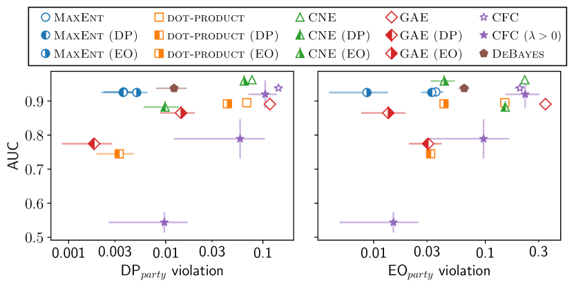
(a) Results on the Polblogs dataset.

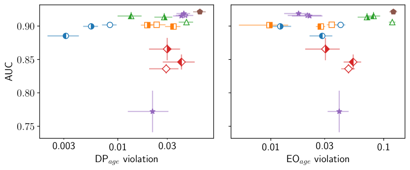
(b) Results on the ML100k dataset.

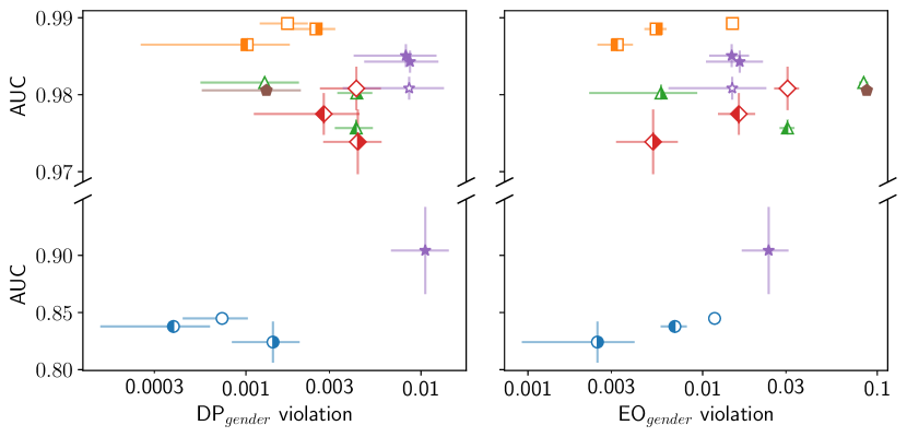
(c) Results on the Facebook dataset.

Figure 1: Markers display the mean over ten identical experiment runs with different random seeds. Error bars horizontally and vertically show the standard deviation. Completely empty markers refer to methods without any fairness modification. Methods with a fairness regularizer that enforces the DP or EO fairness criterion are left-filled or right-filled respectively. On the x-axis, unfairness is measured, so more left is better. On the y-axis, AUC is measured, so higher is better.

The test set results are reported in Fig. 1. We reiterate that our intention is not to find the specific link prediction method with the best trade-off in terms of AUC and fairness. Rather, we want to verify that our proposed regularizer can be applied to a variety of methods and fairness criteria, with an efficient AUC-fairness trade-off for the considered criterion.

Fairness Quality: In many cases and across all four methods, it can indeed be observed that the use of our proposed fairness regularizer significantly reduces the link prediction bias, according to the employed fairness criteria. This is in contrast to the baselines DeBayes and CFC. The former did not improve fairness scores over CNE, while the latter could only become more fair at a significant cost to AUC.

There are a few exceptions where our method does not reduce unfairness according to the fairness criterion. First, there are some cases where an already low DP score for the base method can not be improved further by adding the DP regularizer. This happens for MaxEnt in Fig. 1(a), GAE and Dot-Product in Fig. 1(b) and for CNE in Fig. 1(c). A second kind of exception is where the method with the DP regularizer is less EO-unfair than with the EO regularizer. It occurs for the Dot-Product (EO) variant in Fig. 1(a) and 1(c), possibly because the former had a larger reduction in predictive power overall. In both these cases, Dot-Product (EO) still significantly reduces EO compared to the Dot-Product model without fairness regularizer.

Predictive Quality: Moreover, the decrease in AUC is fairly minimal with our fairness regularizer, especially compared to an adversarial approach like CFC. While the addition of the EO regularizer has no noticeable effect on the AUC, the DP variant does cause strong reduction on some models in Fig. 1(a). This is to be expected, because enforcing DP can cause a significant loss in predictive power if the subgroups in the underlying data have different base rates [15]. For a network like Polblogs, which strongly favors intra-group connections, encouraging the inter-group connections therefore results in AUC loss.

Runtimes: Runtimes of each method are listed in Tab. 3. In our experiments, the addition of our regularizer causes a large increase in runtime. However, several easy speed improvements are available to make the method scale to large graphs. For example, the optimal $\lambda$ parameters of $h_{\mathcal{F}}$ can be approximated by only fitting them on a subsample of the vertex pairs that $h$ is trained on. As shown in Fig. 3, the resulting KL-divergence (computed over all vertex samples that are available to $h$), is already a good estimate when relatively small subsample sizes were used.

Dataset	Polblogs	ML100k	Facebook
MaxEnt	14	68	158
with MA	707	3050	1924
with EO	170	773	1191
Dot-Product	60	62	200
with DP	349	456	1169
with EO	135	239	531
CNE	105	307	349
with DP	574	1417	2065
with EO	286	843	865
CNE	28	26	101
with DP	278	437	1072
with EO	92	255	388
CFC	280	843	1601
CFC $(\lambda>0)$	242	2623	3494
DeBayes	98	305	343

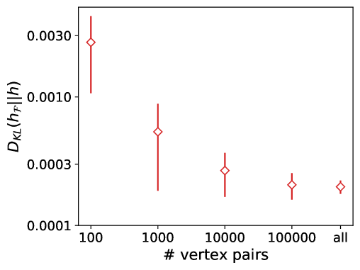
Figure 2: Median runtimes (s) measured by Python’s time.perf_counter.

Figure 3: The KL-divergence in the experiment of Fig. 1(c) between GAE and its fair I-projection, trained using samples from the set of all considered vertex pairs during training: all training edges plus 100 negative edges per vertex.

6 Conclusion

Employing a generic way to characterize the set of fair link prediction distributions, we can compute the I-projection of any graph model onto this set. That distance, i.e. the KL-divergence between the model and its I-projection, can then be used as a principled regularizer during the training process and can be applied to a wide range of statistical fairness criteria. We evaluated the benefit of our proposed method for two such criteria: demographic parity and equalized opportunity.

Overall, our regularizer caused significant improvements in the desired fairness notions, at a relatively minimal cost in predictive power. In this it outperformed the baseline fairness modifications for graph embedding methods, which could not leverage its debiased embeddings to perform fair link prediction according to generic fairness criteria. In the future, more task-specific link prediction fairness criteria can be defined within our framework, taking inspiration from social graph or recommender systems literature. Moreover, our proposed regularizer can be extended beyond graph data structures.

Appendix

A Hyperparameters and Implementation

As stated in the paper, hyperparameter tuning was minimal. In this section, we nevertheless provide, for each method, additional details on the choice of hyperparameters and implementations. The source code is also provided in the supplementary submission.

MaxEnt
The MaxEnt model is used in both the CNE and DeBayes models as a prior distribution. We therefore used the code available for CNE (available here) as a starting point for developing a PyTorch version of this model. The optimisation was done with LBFGS, with at most 100 iterations.

Dot-Product
Due to the simplicity of the Dot-Product model, it was implemented from scratch in PyTorch. A dimensionality of $128$ performed the best among the considered values $\{8,16,128\}$. The model was optimised with Adam and at a learning rate of $0.01$ with $100$ iterations.

CNE
The CNE implementation was based on the code from DeBayes, since the latter is a fairness adaptation of CNE. Our PyTorch modification was made similar to Dot-Product, except that it uses the distance between node embeddings instead of the actual dot product, and it uses MaxEnt as a prior distribution. As hyperparameters, we used the default values as listed for DeBayes: dimensionality of $8$, learning rate of $0.1$ and $s_{2}$ value of $16$. However, we found the method already converged with $200$ epochs, as opposed to the default $1000$.

GAE
For the GAE implementation, we closely followed the source code here. We used similar parameters as Dot-Product, but found a dimensionality of $16$ achieved better validation scores.

CFC
We applied the CFC method to link prediction by using it as a dot-product decoder. As such, the hyperparameters are the same as for Dot-Product, though we stayed as close as possible to the original implementation available here.

DeBayes
Our implementation of DeBayes is based on the publicly available version here. However, we used our own PyTorch version of CNE in order to compare both methods easily. The DeBayes method has no other hyperparameters besides those listed for CNE.

B Additional Measures

In addition to the DP and EO measures, we evaluated the considered methods on two additional fairness measures.

Rank DP (RDP)
As stated in the paper, we computed the DP measure as the maximum difference between the mean link prediction probability of each subgroup combination, proposed in prior work [6]. A possible drawback of this approach is that an algorithm can reduce its DP score by simply making all prediction probabilities very similar. For example, a dot-product decoder may give privileged vertex pairs a link probability of $0.9$, and unprivileged pairs a score of $0.5$. Such a method would have a DP score of $0.4$. However, e.g. by rescaling the embeddings, a similar dot-product decoder may predict scores of $0.6$ and $0.5$ for privileged and unprivileged pairs respectively, which would result in a DP score of $0.1$. Both methods provide total separation in the ranks of the scores between subgroups, so it could be argued that they are both extremely (yet equally) discriminatory.

Taking inspiration from prior work [kallus2019fairness], consider the AUC score, computed over the link prediction scores on the test set, when pairs of vertices of sensitive groups $V_{s}$ and $V_{t}$ respectively are the positive class and vertices with a different sensitive attribute combination are the negative class. Let the Rank Demographic Parity (RDP) score be the maximum of those AUC scores, over all sensitive value pairs $(s,t)\in S$. Clearly, when the prediction scores are completely separated between groups as in the earlier example, the RDP score would equal $1$.

In the results reported in Sec. C, the RDP score heavily correlated with the DP score, suggesting that the latter is already an adequate measure of demographic parity in our experiment setup.

Representation Bias (RB)
The baseline methods DeBayes [6] and CFC [4] focus on making the embeddings themselves less biased. While this was not the direct aim of our fairness regularizer, we evaluate all considered methods by also measuring the Representation Bias (RB) [6], i.e. the maximum AUC score that a logistic regression classifier achieves when it attempts to predict the sensitive attribute value of a vertex’ embedding.

We report the scores using such an evaluation measure in Sec. C and validate that DeBayes and CFC indeed succeed in debiasing their embeddings, as reported in their respective papers. The hyperparameters of the classifier are tuned on a validation set of vertices among all vertices in the graph. In some cases, e.g. for Dot-Product (DP), the optimal hyperparameters are those that cause extreme regularisation, causing the RB scores to be $0.5$.

C Results in Table Format

The full experimental results, which were displayed as AUC-fairness trade-offs in the paper, are again displayed in Tab. 2, 3 and 4. In addition to the DP and EO fairness measures, the RDP and RB scores as described in Sec. B are also listed.

Table 2: Mean $\pm$ standard deviation of results on the polblogs dataset.

Method	AUC	DP	EO	RDP	RB
CFC	0.938 $\pm$ 0.0047	0.145 $\pm$ 0.0151	0.204 $\pm$ 0.0211	0.664 $\pm$ 0.0154	0.977 $\pm$ 0.0049
CFC $(\lambda=10)$	0.920 $\pm$ 0.0407	0.106 $\pm$ 0.0346	0.228 $\pm$ 0.0766	0.668 $\pm$ 0.0336	0.940 $\pm$ 0.1194
CFC $(\lambda=100)$	0.789 $\pm$ 0.0578	0.058 $\pm$ 0.0463	0.096 $\pm$ 0.0662	0.626 $\pm$ 0.0442	0.859 $\pm$ 0.1188
CFC $(\lambda=1000)$	0.544 $\pm$ 0.0297	0.010 $\pm$ 0.0071	0.015 $\pm$ 0.0101	0.520 $\pm$ 0.0135	0.595 $\pm$ 0.0482
CNE	0.962 $\pm$ 0.0022	0.077 $\pm$ 0.0033	0.226 $\pm$ 0.0079	0.679 $\pm$ 0.0063	0.979 $\pm$ 0.0095
CNE (DP)	0.882 $\pm$ 0.0045	0.010 $\pm$ 0.0039	0.151 $\pm$ 0.0080	0.577 $\pm$ 0.0058	0.765 $\pm$ 0.0284
CNE (EO)	0.959 $\pm$ 0.0022	0.064 $\pm$ 0.0027	0.043 $\pm$ 0.0105	0.651 $\pm$ 0.0094	0.971 $\pm$ 0.0102
DeBayes	0.937 $\pm$ 0.0026	0.012 $\pm$ 0.0042	0.065 $\pm$ 0.0074	0.615 $\pm$ 0.0067	0.699 $\pm$ 0.0524
Dot-Product	0.895 $\pm$ 0.0035	0.068 $\pm$ 0.0021	0.149 $\pm$ 0.0056	0.738 $\pm$ 0.0070	0.975 $\pm$ 0.0062
Dot-Product (DP)	0.745 $\pm$ 0.0046	0.003 $\pm$ 0.0014	0.032 $\pm$ 0.0016	0.570 $\pm$ 0.0083	0.500 $\pm$ 0.0000
Dot-Product (EO)	0.892 $\pm$ 0.0037	0.043 $\pm$ 0.0016	0.043 $\pm$ 0.0034	0.657 $\pm$ 0.0076	0.946 $\pm$ 0.0069
GAE	0.891 $\pm$ 0.0031	0.118 $\pm$ 0.0035	0.346 $\pm$ 0.0309	0.753 $\pm$ 0.0138	0.983 $\pm$ 0.0061
GAE (DP)	0.775 $\pm$ 0.0091	0.002 $\pm$ 0.0010	0.031 $\pm$ 0.0100	0.583 $\pm$ 0.0143	0.825 $\pm$ 0.0419
GAE (EO)	0.865 $\pm$ 0.0135	0.014 $\pm$ 0.0056	0.014 $\pm$ 0.0058	0.648 $\pm$ 0.0194	0.972 $\pm$ 0.0061
MaxEnt	0.927 $\pm$ 0.0026	0.004 $\pm$ 0.0014	0.036 $\pm$ 0.0061	0.617 $\pm$ 0.0070	/
MaxEnt (DP)	0.925 $\pm$ 0.0028	0.004 $\pm$ 0.0015	0.033 $\pm$ 0.0065	0.617 $\pm$ 0.0084	/
MaxEnt (EO)	0.925 $\pm$ 0.0038	0.005 $\pm$ 0.0014	0.009 $\pm$ 0.0047	0.604 $\pm$ 0.0042	/

Table 3: Mean $\pm$ standard deviation of results on the ml100k dataset.

Method	AUC	DP	EO	RDP	RB
CFC	0.916 $\pm$ 0.0021	0.045 $\pm$ 0.0086	0.021 $\pm$ 0.0070	0.531 $\pm$ 0.0040	0.631 $\pm$ 0.0191
CFC $(\lambda=10)$	0.919 $\pm$ 0.0021	0.043 $\pm$ 0.0065	0.018 $\pm$ 0.0045	0.530 $\pm$ 0.0030	0.662 $\pm$ 0.0127
CFC $(\lambda=100)$	0.915 $\pm$ 0.0023	0.041 $\pm$ 0.0069	0.022 $\pm$ 0.0066	0.530 $\pm$ 0.0036	0.681 $\pm$ 0.0158
CFC $(\lambda=1000)$	0.772 $\pm$ 0.0311	0.022 $\pm$ 0.0092	0.040 $\pm$ 0.0085	0.519 $\pm$ 0.0035	0.547 $\pm$ 0.0235
CNE	0.906 $\pm$ 0.0015	0.046 $\pm$ 0.0073	0.119 $\pm$ 0.0078	0.536 $\pm$ 0.0030	0.547 $\pm$ 0.0123
CNE (DP)	0.915 $\pm$ 0.0013	0.013 $\pm$ 0.0035	0.081 $\pm$ 0.0117	0.511 $\pm$ 0.0020	0.588 $\pm$ 0.0205
CNE (EO)	0.913 $\pm$ 0.0014	0.028 $\pm$ 0.0055	0.071 $\pm$ 0.0124	0.528 $\pm$ 0.0032	0.614 $\pm$ 0.0134
DeBayes	0.921 $\pm$ 0.0013	0.062 $\pm$ 0.0086	0.122 $\pm$ 0.0096	0.536 $\pm$ 0.0028	0.524 $\pm$ 0.0235
Dot-Product	0.902 $\pm$ 0.0012	0.024 $\pm$ 0.0051	0.035 $\pm$ 0.0033	0.528 $\pm$ 0.0029	0.657 $\pm$ 0.0233
Dot-Product (DP)	0.899 $\pm$ 0.0012	0.034 $\pm$ 0.0058	0.028 $\pm$ 0.0026	0.509 $\pm$ 0.0037	0.759 $\pm$ 0.0232
Dot-Product (EO)	0.901 $\pm$ 0.0012	0.019 $\pm$ 0.0026	0.010 $\pm$ 0.0045	0.526 $\pm$ 0.0029	0.697 $\pm$ 0.0275
GAE	0.836 $\pm$ 0.0072	0.029 $\pm$ 0.0092	0.049 $\pm$ 0.0067	0.518 $\pm$ 0.0040	0.582 $\pm$ 0.0279
GAE (DP)	0.846 $\pm$ 0.0112	0.041 $\pm$ 0.0140	0.054 $\pm$ 0.0094	0.510 $\pm$ 0.0050	0.645 $\pm$ 0.0195
GAE (EO)	0.866 $\pm$ 0.0167	0.030 $\pm$ 0.0100	0.030 $\pm$ 0.0103	0.517 $\pm$ 0.0034	0.578 $\pm$ 0.0325
MaxEnt	0.902 $\pm$ 0.0014	0.008 $\pm$ 0.0014	0.042 $\pm$ 0.0040	0.536 $\pm$ 0.0026	/
MaxEnt (DP)	0.885 $\pm$ 0.0039	0.003 $\pm$ 0.0011	0.029 $\pm$ 0.0065	0.515 $\pm$ 0.0055	/
MaxEnt (EO)	0.899 $\pm$ 0.0013	0.006 $\pm$ 0.0009	0.012 $\pm$ 0.0030	0.530 $\pm$ 0.0018	/

Table 4: Mean $\pm$ standard deviation of results on the facebook dataset.

Method	AUC	DP	EO	RDP	RB
CFC	0.981 $\pm$ 0.0015	0.009 $\pm$ 0.0050	0.015 $\pm$ 0.0084	0.529 $\pm$ 0.0068	0.601 $\pm$ 0.0150
CFC $(\lambda=10)$	0.984 $\pm$ 0.0014	0.009 $\pm$ 0.0039	0.016 $\pm$ 0.0058	0.529 $\pm$ 0.0040	0.615 $\pm$ 0.0153
CFC $(\lambda=100)$	0.985 $\pm$ 0.0015	0.008 $\pm$ 0.0041	0.015 $\pm$ 0.0038	0.529 $\pm$ 0.0049	0.617 $\pm$ 0.0157
CFC $(\lambda=1000)$	0.904 $\pm$ 0.0381	0.011 $\pm$ 0.0038	0.024 $\pm$ 0.0071	0.532 $\pm$ 0.0052	0.586 $\pm$ 0.0228
CNE	0.982 $\pm$ 0.0006	0.001 $\pm$ 0.0007	0.084 $\pm$ 0.0050	0.538 $\pm$ 0.0035	0.601 $\pm$ 0.0189
CNE (DP)	0.976 $\pm$ 0.0006	0.004 $\pm$ 0.0010	0.031 $\pm$ 0.0030	0.512 $\pm$ 0.0027	0.594 $\pm$ 0.0217
CNE (EO)	0.980 $\pm$ 0.0006	0.004 $\pm$ 0.0010	0.006 $\pm$ 0.0035	0.518 $\pm$ 0.0025	0.607 $\pm$ 0.0192
DeBayes	0.981 $\pm$ 0.0004	0.001 $\pm$ 0.0007	0.087 $\pm$ 0.0042	0.539 $\pm$ 0.0030	0.592 $\pm$ 0.0163
Dot-Product	0.989 $\pm$ 0.0006	0.002 $\pm$ 0.0005	0.015 $\pm$ 0.0007	0.561 $\pm$ 0.0037	0.630 $\pm$ 0.0138
Dot-Product (DP)	0.987 $\pm$ 0.0008	0.001 $\pm$ 0.0008	0.003 $\pm$ 0.0007	0.515 $\pm$ 0.0032	0.500 $\pm$ 0.0000
Dot-Product (EO)	0.989 $\pm$ 0.0005	0.003 $\pm$ 0.0007	0.005 $\pm$ 0.0008	0.530 $\pm$ 0.0041	0.769 $\pm$ 0.0185
GAE	0.981 $\pm$ 0.0028	0.004 $\pm$ 0.0016	0.031 $\pm$ 0.0050	0.545 $\pm$ 0.0037	0.602 $\pm$ 0.0152
GAE (DP)	0.977 $\pm$ 0.0027	0.003 $\pm$ 0.0017	0.016 $\pm$ 0.0039	0.518 $\pm$ 0.0061	0.626 $\pm$ 0.0193
GAE (EO)	0.974 $\pm$ 0.0042	0.004 $\pm$ 0.0016	0.005 $\pm$ 0.0020	0.535 $\pm$ 0.0026	0.618 $\pm$ 0.0240
MaxEnt	0.845 $\pm$ 0.0014	0.001 $\pm$ 0.0003	0.012 $\pm$ 0.0007	0.541 $\pm$ 0.0041	/
MaxEnt (DP)	0.838 $\pm$ 0.0043	0.000 $\pm$ 0.0002	0.007 $\pm$ 0.0012	0.530 $\pm$ 0.0051	/
MaxEnt (EO)	0.824 $\pm$ 0.0180	0.001 $\pm$ 0.0006	0.002 $\pm$ 0.0016	0.519 $\pm$ 0.0070	/

References

- [1] Adamic, L.A., Glance, N.: The political blogosphere and the 2004 us election: divided they blog. In: Proceedings of the 3rd international workshop on Link discovery. pp. 36–43 (2005)
- [2] Agarwal, A., Beygelzimer, A., Dudík, M., Langford, J., Wallach, H.: A reductions approach to fair classification. In: International Conference on Machine Learning. pp. 60–69. PMLR (2018)
- [3] Alghamdi, W., Asoodeh, S., Wang, H., Calmon, F.P., Wei, D., Ramamurthy, K.N.: Model projection: Theory and applications to fair machine learning. In: 2020 IEEE International Symposium on Information Theory (ISIT). pp. 2711–2716. IEEE (2020)
- [4] Bose, A., Hamilton, W.: Compositional fairness constraints for graph embeddings. In: International Conference on Machine Learning. pp. 715–724 (2019)
- [5] Burnham, K.P., Anderson, D.R.: Practical use of the information-theoretic approach. In: Model selection and inference, pp. 75–117. Springer (1998)
- [6] Buyl, M., De Bie, T.: Debayes: a bayesian method for debiasing network embeddings. In: International Conference on Machine Learning. pp. 1220–1229. PMLR (2020)
- [7] Calmon, F.P., Wei, D., Vinzamuri, B., Ramamurthy, K.N., Varshney, K.R.: Optimized pre-processing for discrimination prevention. In: Proceedings of the 31st International Conference on Neural Information Processing Systems. pp. 3995–4004 (2017)
- [8] Cotter, A., Jiang, H., Gupta, M.R., Wang, S., Narayan, T., You, S., Sridharan, K.: Optimization with non-differentiable constraints with applications to fairness, recall, churn, and other goals. Journal of Machine Learning Research 20(172), 1–59 (2019)
- [9] Cover, T.M.: Elements of information theory. John Wiley & Sons (1999)
- [10] Csiszár, I.: I-divergence geometry of probability distributions and minimization problems. The annals of probability pp. 146–158 (1975)
- [11] Csiszár, I., Matus, F.: Information projections revisited. IEEE Transactions on Information Theory 49(6), 1474–1490 (2003)
- [12] De Bie, T.: Maximum entropy models and subjective interestingness: an application to tiles in binary databases. Data Mining and Knowledge Discovery 23(3), 407–446 (2011)
- [13] Dwork, C., Hardt, M., Pitassi, T., Reingold, O., Zemel, R.: Fairness through awareness. In: Proceedings of the 3rd innovations in theoretical computer science conference. pp. 214–226 (2012)
- [14] Hamilton, W.L., Ying, R., Leskovec, J.: Representation learning on graphs: Methods and applications. arXiv preprint arXiv:1709.05584 (2017)
- [15] Hardt, M., Price, E., Srebro, N.: Equality of opportunity in supervised learning. In: Proceedings of the 30th International Conference on Neural Information Processing Systems. pp. 3323–3331 (2016)
- [16] Hofstra, B., Corten, R., Van Tubergen, F., Ellison, N.B.: Sources of segregation in social networks: A novel approach using facebook. American Sociological Review 82(3), 625–656 (2017)
- [17] Jiang, H., Nachum, O.: Identifying and correcting label bias in machine learning. In: International Conference on Artificial Intelligence and Statistics. pp. 702–712. PMLR (2020)
- [18] Kang, B., Lijffijt, J., De Bie, T.: Conditional network embeddings. In: International Conference on Learning Representations (2018)
- [19] Karimi, F., Génois, M., Wagner, C., Singer, P., Strohmaier, M.: Homophily influences ranking of minorities in social networks. Scientific reports 8(1), 1–12 (2018)
- [20] Kipf, T.N., Welling, M.: Variational graph auto-encoders. arXiv preprint arXiv:1611.07308 (2016)
- [21] Laclau, C., Redko, I., Choudhary, M., Largeron, C.: All of the fairness for edge prediction with optimal transport. In: International Conference on Artificial Intelligence and Statistics. pp. 1774–1782. PMLR (2021)
- [22] Li, P., Wang, Y., Zhao, H., Hong, P., Liu, H.: On dyadic fairness: Exploring and mitigating bias in graph connections. In: International Conference on Learning Representations (2021)
- [23] Liben-Nowell, D., Kleinberg, J.: The link-prediction problem for social networks. Journal of the American society for information science and technology 58(7), 1019–1031 (2007)
- [24] Martínez, V., Berzal, F., Cubero, J.C.: A survey of link prediction in complex networks. ACM computing surveys (CSUR) 49(4), 1–33 (2016)
- [25] Masrour, F., Wilson, T., Yan, H., Tan, P.N., Esfahanian, A.: Bursting the filter bubble: Fairness-aware network link prediction. In: Proceedings of the AAAI Conference on Artificial Intelligence. vol. 34, pp. 841–848 (2020)
- [26] McAuley, J., Leskovec, J.: Learning to discover social circles in ego networks. In: Proceedings of the 25th International Conference on Neural Information Processing Systems. pp. 539–547 (2012)
- [27] McPherson, M., Smith-Lovin, L., Cook, J.M.: Birds of a feather: Homophily in social networks. Annual review of sociology 27(1), 415–444 (2001)
- [28] Mehrabi, N., Morstatter, F., Saxena, N., Lerman, K., Galstyan, A.: A survey on bias and fairness in machine learning. arXiv preprint arXiv:1908.09635 (2019)
- [29] Rahman, T., Surma, B., Backes, M., Zhang, Y.: Fairwalk: Towards fair graph embedding. In: Proceedings of the Twenty-Eighth International Joint Conference on Artificial Intelligence, IJCAI-19. pp. 3289–3295. International Joint Conferences on Artificial Intelligence Organization (2019)
- [30] Robins, G., Pattison, P., Kalish, Y., Lusher, D.: An introduction to exponential random graph (p*) models for social networks. Social networks 29(2), 173–191 (2007)
- [31] Wei, D., Ramamurthy, K.N., Calmon, F.: Optimized score transformation for fair classification. In: International Conference on Artificial Intelligence and Statistics. pp. 1673–1683. PMLR (2020)
- [32] Woodworth, B., Gunasekar, S., Ohannessian, M.I., Srebro, N.: Learning non-discriminatory predictors. In: Conference on Learning Theory. pp. 1920–1953. PMLR (2017)
- [33] Wu, Z., Pan, S., Chen, F., Long, G., Zhang, C., Philip, S.Y.: A comprehensive survey on graph neural networks. IEEE transactions on neural networks and learning systems (2020)
- [34] Zafar, M.B., Valera, I., Rogriguez, M.G., Gummadi, K.P.: Fairness constraints: Mechanisms for fair classification. In: Artificial Intelligence and Statistics. pp. 962–970. PMLR (2017)
- [35] Zhang, M., Chen, Y.: Link prediction based on graph neural networks. In: Proceedings of the 32nd International Conference on Neural Information Processing Systems. pp. 5171–5181 (2018)