The Rediscovery Hypothesis:
Language Models Need to Meet Linguistics

Abstract

There is an ongoing debate in the NLP community whether modern language models contain linguistic knowledge, recovered through so-called probes. In this paper, we study whether linguistic knowledge is a necessary condition for the good performance of modern language models, which we call the rediscovery hypothesis.

In the first place, we show that language models that are significantly compressed but perform well on their pretraining objectives retain good scores when probed for linguistic structures. This result supports the rediscovery hypothesis and leads to the second contribution of our paper: an information-theoretic framework that relates language modeling objectives with linguistic information. This framework also provides a metric to measure the impact of linguistic information on the word prediction task. We reinforce our analytical results with various experiments, both on synthetic and on real NLP tasks in English.

1 Introduction

Vector representations of words obtained from self-supervised pretraining of neural language models (LMs) on massive unlabeled data have revolutionized NLP in the last decade. This success has spurred an interest in trying to understand what type of knowledge these models actually learn (?, ?).

Of particular interest here is “linguistic knowledge”, which is generally measured by annotating test sets through experts (linguists) following certain pre-defined linguistic schemas. These annotation schemas are based on language regularities manually defined by linguists. On the other side, we have language models which are pretrained predictors that assign a probability to the presence of a token given the surrounding context. Neural models solve this task by finding patterns in the text. We refer to the claim that such neural language models rediscover linguistic knowledge as the rediscovery hypothesis. It stipulates that the patterns of the language discovered by the model trying to solve the pretraining task correlate with the human-defined linguistic regularity. In this work we measure the amount of linguistics rediscovered by a pretrained model through the so-called probing tasks: hidden layers of a neural LM are fed to a simple classifier—a probe—that learns to predict a linguistic structure of interest (?, ?, ?, ?, ?). In the first part of this paper (Section 2) we attempt to challenge the rediscovery hypothesis through a variety of experiments to understand to what extent it holds. Those experiments aim to verify whether the path through language regularity is indeed the one taken by pretrained LMs or whether there is another way to reach good LM performance without rediscovering linguistic structure. Our experiments show that pretraining loss is indeed tightly linked to the amount of linguistic structure discovered by an LM. We, therefore, fail to reject the rediscovery hypothesis.

This negative attempt, as well as the abundance of positive examples in the literature, motivates us to prove mathematically the rediscovery hypothesis. In the second part of our paper (Section 3) we use information theory to prove the contrapositive of the hypothesis—removal of linguistic information from an LM degrades its performance. Moreover, we show that the decline in the LM quality depends on how strongly the removed property is interdependent with the underlying text: a greater dependence leads to a greater drop. We confirm this result empirically, both with synthetic data and with real annotations on English text.

The result that removing information that contains strong mutual information with the underlying text degrades (masked) word prediction might not seem surprising a posteriori. However, it is this surprise that lies at the heart of most of the work in recent years around the discovery of how easily this information can be extracted from intermediate representations. Our framework also provides a coefficient that measures the dependence between a probing task and the underlying text. This measure can be used to determine more complex probing tasks, whose rediscovery by language models would indeed be surprising.

2 Do Pretraining Objectives Correlate with Linguistic Structures?

The first question we pose in this work is the following: is the rediscovery of linguistic knowledge mandatory for models that perform well on their pretraining tasks, typically language modeling or translation; or is it a side effect of overparameterization?

We analyze the correlation between linguistic knowledge and LM performance with pruned pretrained models. By compressing a network through pruning we retain the same overall architecture and can compare probing methods. More important, we hypothesize that pruning removes all unnecessary information with respect to the pruning objective (language modeling) and that it might be that information that is used to rediscover linguistic knowledge. To complete this experiment, we also track the pruning efficiency during pretraining.

2.1 Pruning Method

The lottery ticket hypothesis (LTH) of ? (?) claims that a randomly-initialized neural network $f(\mathbf{x};\boldsymbol{\theta})$ with trainable parameters $\boldsymbol{\theta}\in\mathbb{R}^{n}$ contains subnetworks $f(\mathbf{x};\mathbf{m}\odot\boldsymbol{\theta})$, $\mathbf{m}\in\{0,1\}^{n}$, such that, when trained in isolation, they can match the performance of the original network. The authors suggest a simple procedure for identifying such subnetworks (Alg. 2.1). When this procedure is applied iteratively (Step 2.1 of Alg. 2.1), we get a sequence of pruned models $\{f(\mathbf{x};\mathbf{m}_{i}\odot\boldsymbol{\theta}_{0})\}$ in which each model has fewer parameters than its predecessor: $\|\mathbf{m}_{i}\|_{0}<\|\mathbf{m}_{i-1}\|_{0}$. ? used iterative pruning for image classification models and found subnetworks that were 10%–20% of the sizes of the original networks and met or exceeded their validation accuracies. Such a compression approach retains weights important for the main task while discarding others. We hypothesize that it might be those additional weights that contain the signals used by probes. But, if the subnetworks retain linguistic knowledge then this is evidence in favor of the rediscovery hypothesis.

1 Randomly initialize a neural network $f(\mathbf{x};\boldsymbol{\theta}_{0})$, $\boldsymbol{\theta}_{0}\in\mathbb{R}^{n}$

2 Train the network for $j$ iterations, arriving at parameters $\boldsymbol{\theta}_{j}$.

3 Prune $p\%$ of the parameters in $\boldsymbol{\theta}_{j}$, creating a mask $\boldsymbol{m}\in\{0,1\}^{n}$.

4 Reset the remaining parameters to their values in $\boldsymbol{\theta}_{0}$, creating the winning ticket $f(\mathbf{x};\boldsymbol{m}\odot\boldsymbol{\theta}_{0})$.

5 Repeat from 2.1 if performing iterative pruning.

Train the winning ticket $f(\mathbf{x};\mathbf{m}\odot\boldsymbol{\theta}_{0})$ to convergence.

Algorithm 2.1 Lottery ticket hypothesis—Identifying winning tickets (?)

2.2 Models

We explore one static embedding model, SGNS, and two contextualized embedding models, CoVe and RoBERTa. In this manner, we cover the full spectrum of modern representations of words, from static embeddings to shallow and deep contextual embeddings.

CoVe (?)

uses the top-level activations of a two-layer BiLSTM encoder from an attentional sequence-to-sequence model (?) trained for English-to-German translation. The authors used the CommonCrawl-840B GloVe model (?) for English word vectors, which were completely fixed during pretraining, and we follow their setup. This entails that the embedding layer on the source side is not pruned during the LTH procedure. We also concatenate the encoder output with the GloVe embeddings as is done in the original paper (?, Eq. 6).

BERT (?)

is a deep Transformer (?) encoder that has become the de facto standard when it comes to contextualized embeddings. We pretrain the RoBERTa variant of the BERT model (?). RoBERTa stands for robustly optimized BERT which was trained with hyperparameters optimized for convergence, with dynamic masking instead of static masking, and restricted to masked LM objective only. Unlike their predecessors, such as CoVe and ELMo (?), BERT and other Transformer-based encoders are considered deep contextualizers.

Word2vec SGNS (?)

is a shallow two-layer neural network that produces uncontextualized word embeddings. It is widely accepted that the SGNS vectors capture words semantics to a certain extent, which is confirmed by the folklore examples, such as $\mathbf{w}_{\text{king}}-\mathbf{w}_{\text{man}}+\mathbf{w}_{\text{woman}}\approx\mathbf{w}_{\text{queen}}$. So, the question of the relationship between the SGNS objective function and its ability to discover linguistics is also relevant.

2.3 Measuring the Amount of Linguistic Knowledge

To properly measure the amount of linguistic knowledge in word vectors we define it as the performance of classifiers (probes) that take those vectors as input and are trained on linguistically annotated data. This definition has the advantage of being able to be measured exactly, at the cost of avoiding the discussion of whether POS tags or syntactic parse trees indeed denote linguistic knowledge captured by humans in their learning process.

We should note that this probing approach has received a lot of criticism recently (?, ?, ?) due to its inability to distinguish between information encoded in the pretrained vectors from the information learned by the probing classifier. However, in our study, the question is not How much linguistics is encoded in the presentation vector?, but rather Does one vector contain more linguistic information than the other? We compare different representations of the same dimensionality using probing classifiers of the same capacity. Even if part of the probing performance is due to the classifier itself we claim that the difference in the probing performance will be due to the difference in the amount of linguistic knowledge encoded in the representations we manipulate. This conjecture is strengthened by the findings of ? (?) who analyzed the representations from pretrained miniBERTas and demonstrated that the trends found through edge probing (?) are the same as those found through better-designed probes such as Minimum Description Length (?). Therefore in our work we adopt edge probing and structural probing for contextualized embeddings. For static embeddings, we use the traditional word similarity and word analogy tasks.

Edge probing (?)

formulates several linguistics tasks of different nature as text span classification tasks. The probing model is a lightweight classifier on top of the pretrained representations trained to solve those linguistic tasks. In our study, we use the part-of-speech tagging (POS), constituent labeling, named entity labeling (NE), and semantic role labeling (SRL) tasks from the suite, in which a probing classifier receives a sequence of tokens and predicts a label for it. For example, in the case of constituent labeling, for a sentence This probe $[\textit{discovers linguistic knowledge}]$, the sequence in square brackets should be labeled as a verb phrase.

Structural probing (?)

evaluates whether syntax trees are embedded in a linear transformation of a neural network’s word representation space. The probe identifies a linear transformation under which squared Euclidean distance encodes the distance between words in the parse tree. ? show that such transformations exist for both ELMo and BERT but not in static baselines, providing evidence that entire syntax trees can be easily extracted from the vector geometry of deep models.

Word similarity (?) and word analogy (?)

tasks can be considered as nonparametric probes of static embeddings, and—differently from the other probing tasks—are not learned. The use of word embeddings in the word similarity task has been criticized for the instability of the results obtained (?). Regarding the word analogy task, ? (?) raised concerns on the misalignment of assumptions in generating and testing word embeddings. However, the success of the static embeddings in performing well in these tasks was a crucial part of their widespread adoption.

2.4 Experimental Setup

We prune the embedding models from Section 2.2 with the LTH algorithm (Alg. 2.1) and evaluate them with probes from Section 2.3 at each pruning iteration. CoVe and SGNS are pruned iteratively, while for RoBERTa we perform one-shot pruning at different rates. Assuming that $\ell^{\omega}_{i}$ is the validation loss of the embedding model $\omega\in\{$CoVe, RoBERTa, SGNS$\}$ at iteration $i$, and $\Delta s^{\omega,T}_{i}:=s^{\omega,T}_{i}-s^{\omega,T}_{0}$ is the drop in the corresponding score on the probing task $T\in\{$NE, POS, Const., Struct., Sim., Analogy$\}$ compared to the score $s^{\omega,T}_{0}$ of the baseline (unpruned) model, we obtain pairs $(\ell^{{\omega}}_{i},\Delta s^{{\omega},{T}}_{i})$ for further analysis. Keep in mind that RoBERTa and SGNS are pruned in full, while in CoVe we prune everything except the source-side embedding layer. This exception is due to the design of the CoVe model, and we follow the original paper’s setup (?).

Software and datasets.

We pretrain CoVe on the English–German part of the IWSLT 2016 machine translation task (?) using the OpenNMT-py toolkit (?). RoBERTa is pretrained on the WikiText-103 dataset (English) (?) using the fairseq toolkit (?) with default training settings (?). Finally, the SGNS model is pretrained on the text8 data (English as well) (?) using our custom implementation (?).

The edge probing classifier is trained on the standard benchmark dataset OntoNotes 5.0 (?) using the jiant toolkit (?). The structural probe is trained on the English UD (?) using the code from the authors (?). For word similarities we use the WordSim353 dataset (?), while for word analogies we use the Google dataset (?). All those datasets are in English.

Optimization

is performed in almost the same way as in the original works on CoVe, RoBERTa, and SGNS. See Appendix A for details.

2.5 Results

First, we note that the lottery ticket hypothesis is confirmed for the embedding models since pruning up to 60% weights does not harm their performance significantly on held-out data (Fig. 3).

Figure 1: Results of applying the LTH (Algorithm 2.1) to CoVe, RoBERTa, and SGNS. In each case we scatter-plot the percentage of remained weights vs validation loss, which is cross entropy for CoVe and RoBERTa, and a variant of negative sampling objective for SGNS.

Figure 2: Probing results for the CoVe and RoBERTa embeddings. Horizontal axes indicate validation loss values, which are cross-entropy values. Vertical axes indicate drops in probing performances. In case of edge probing, we use the NE, POS, and constituent labeling tasks from the suite of ? (?) and report the drop in micro-averaged F1 score compared to the baseline (unpruned) model. In case of structural probing, we use the distance probe of ? (?) and report the drop in undirected unlabeled attachment score (UUAS).

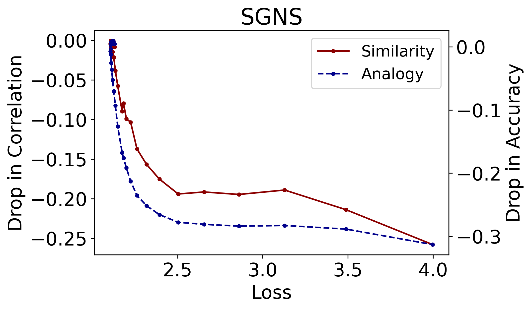
Figure 3: Similarity and analogy results for the SGNS embeddings. For similarities we report the drop in Spearman’s correlation with the human ratings and for analogies in accuracy.

Before proceeding to the results of probing of pruned models, we want to note that the probing scores of the baseline (unpruned) models obtained by us are close to the scores from the original papers (?, ?), and are shown in Table 1.

Model	Task
	NE	POS	Const.	Struct.
CoVe	.921	.936	.808	.726
RoBERTa	.932	.951	.808	.719

Model	Task
	Similarity	Analogy
SGNS	.716	.332

Table 1: Probing scores for the baseline (unpruned) models. We report the micro-averaged F1 score for the POS, NE, and Constituents; undirected unlabeled attachment score (UUAS) for the structural probe; Spearman’s correlation with the human ratings for the similarity task; and accuracy for the analogy task.

Probing results are provided in Fig. 3 and 3, where we scatter-plot validation loss $\ell^{{\omega}}_{i}$ vs drop in probing performance $\Delta s^{{\omega},{T}}_{i}$ for each of the model-probe combinations. First, we note that, in most cases, the probing score correlates with the pretraining loss, which supports the rediscovery hypothesis. We note that the probing score decreases slower for some tasks (e.g., POS tagging), but is much steeper for others (e.g., constituents labeling). This is complementary to the findings of ? (?) who showed that the syntactic learning curve reaches plateau performance with less pretraining data while solving semantic tasks requires more training data. Our results suggest that similar behavior emerges with respect to the model size: simpler tasks (e.g., POS tagging) can be solved with smaller models, while more complex linguistic tasks (e.g., syntactic constituents or dependency parsing) require bigger model size. In addition, we note that in the case of CoVe, and in contrast to RoBERTa, the probing scores for more local (i.e. less context-dependent) tasks such as POS and NER hardly decrease with an increase in the pruning rate. We believe that this is because CoVe representations by default contain unpruned static GloVe embeddings, which by themselves already obtain good performance on the more local tasks.

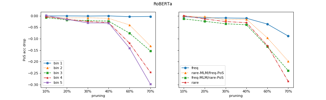
Figure 4: Breakdown of POS tagging accuracy decrease by token frequency. We report the drop in accuracy compared to the baseline (unpruned) model. Left: all bins (1-5) have comparable cumulative counts in the pretraining data. The distribution of tokens over the bins: bin 1 — 5 tokens, bin 2 — 25 tokens, bin 3 — 368 tokens, bin 4 — 2813 tokens, bin 5 — 600K tokens. Right: 4 bins of tokens which are (1) frequent both in pretraining and POS training data (153 tokens), (2) rare in pretraining but frequent in POS training data (66 tokens), (3) frequent in pretraining but rare in POS training data (235 tokens), and (4) rare everywhere (46K tokens).

The reader might have noted that in the case of CoVe in Fig. 3 when the range of $\ell_{i}$’s is restricted to low values, there is a lack of correlation between $\ell_{i}$ and $\Delta s_{i}$. We discuss this further in Appendix B as we argue that this does not contradict our main finding.

Breakdown by token frequency.

The pervasiveness of Zipf’s law in language has the consequence that many conclusions over aggregated scores can be attributed to effects on a small set of tokens. Indeed, when binning tokens by their frequency in the pretraining data and analyzing the POS accuracy drop per bin it becomes obvious that the less frequent a token is the more pruning affects its POS-tag prediction. This is shown in Fig. 4 (left) where tokens are binned in 5 equally-sized groups.

A straightforward interpretation of such behavior would be: (1) pruning degrades the representations for rarer tokens in the first place. It is also possible, that (2) pruning degrades all token representations similarly; however, the probing model has the capacity to recover the POS performance for tokens that are frequent in POS tagging corpus but cannot do that for rare tokens. The first reason would support the claim that pruning removes the memorization for rare tokens, while the second reason would mean that the pruned model redistributes its representation power across all the token groups to preserve good LM performance. The latter behavior would be more aligned with the rediscovery hypothesis.

To better understand which of the two is a better explanation we need to distinguish between tokens which are rare in the pretraining data but are frequent in the downstream POS training data and vice-versa: the behavior on tokens which are rare in POS training data will be more informative of how pruning affects pretrained representations.

For this, we group the first three bins together in a freq-MLM group and the two last bins inside rare-MLM; and do a similar split based on the frequency of the tokens in the POS training corpus (freq-POS and rare-POS).

The impact of pruning on the four possible combinations of groups is shown in Fig. 4 (right). The probing performance on the tokens which are frequent in POS tagging corpus (freq and rare-MLM/freq-POS) keep almost constant up to a pruning rate of 40%. While tokens which are rare in POS tagging corpus (freq-MLM/rare-POS and rare) seem to suffer more with pruning rate growth. This lends support to the possibility that the amount of linguistics contained in the pretrained vectors decreases across all the token groups.

Finally, we note that up to 60% of pruning both freq-MLM/rare-PoS and rare groups behave similarly but at 70% pruning rate the tokens that are rare everywhere (rare) suffer from a higher drop, compared to freq-MLM/rare-PoS meaning that probing model is not able to recover the correct PoS tags for rare tokens. This suggests that memorization gets removed from the pretrained model at a higher pruning rate, but it is exploited by the probing model at lower pruning rates.

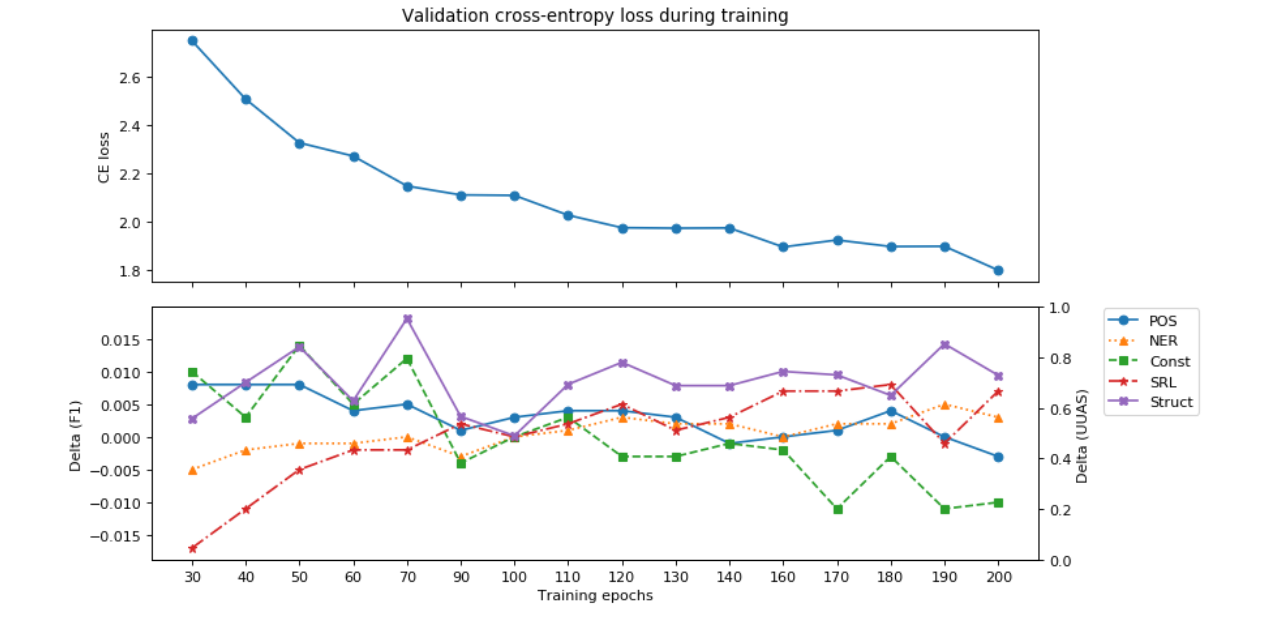
Figure 5: Probing intermediate checkpoints of RoBERTa. Top: RoBERTa validation CE loss during training. Bottom: Difference between the baseline probing score and probing score at each epoch (up to 200). In case of edge probing, we use the SRL, NE, POS, and constituent labeling tasks from the suite of ? (?) and report the micro-averaged F1 score. In case of structural probing, we use the distance probe of ? (?) and report the undirected unlabeled attachment score (UUAS).

2.6 Probing Intermediate Checkpoints

Until now we measured correlated probing accuracy on top of fully-trained models with the amount of pruning those models underwent. Here we use a complementary lens, by analyzing how quickly a pretrained model discovers different types of linguistic knowledge? For this, we save intermediate checkpoints of RoBERTa models and probe those. Similar to pruning, this has the advantage that all models share the same architecture. The results of the probing accuracy over different epochs are provided in Fig. 10.

Similar to ? (?), we find that syntactic tasks (e.g., POS tagging, dependency, and constituency parsing) seem to reach the top probing performance at the beginning of training (30-60 epochs), while semantic tasks (e.g., NER, SRL) keep improving further. While ? (?) argued that “BERT rediscovers NLP pipeline” by looking at intermediate layers of a fully pretrained model, the same seems to apply during the training: linguistic knowledge to solve lexical tasks are learned first while more complex tasks are easier solved with representation obtained later in the learning.

Inter-Section Interlude

We conclude that in general the rediscovery hypothesis seems valid: when language models reach good performance they indeed capture linguistic structures (at least in the case of the English language). So we obtained a negative result when we tried to reject the rediscovery hypothesis. Along with this, positive examples are abundant, including the extensive literature on probing (of which we give an overview in Section 4). This might indicate that the hypothesis is indeed true. The lack of correlation between probing scores and LM performance for one of the considered models only questions the probing methodology but does not reject the very fundamental connection between language modeling and learning linguistic structures. We address this in the next section, where we formalize the connection and show how it holds empirically. The empirical experiments will consist in adversarially removing information that could serve probing accuracy while keeping good LM performance.

3 An Information-Theoretic Framework

Recall that the rediscovery hypothesis asserts that neural language models, in the process of their pretraining, rediscover linguistic knowledge. We will prove this claim by contraposition, which states that without linguistic knowledge, the neural LMs cannot perform at their best. A recent paper of ? (?) has already investigated how linearly removing certain linguistic information from BERT’s layers impacts its accuracy of predicting a masked token. They showed empirically that dependency information, part-of-speech tags, and named entity labels are important for word prediction, while syntactic constituency boundaries (which mark the beginning and the end of a phrase) are not. One of the questions raised by the authors is how to quantify the relative importance of different properties encoded in the representation for the word prediction task. The current section of our work attempts to answer this question—we provide a metric $\rho$ that is a reliable predictor of such importance. This metric occurs naturally when we take an information-theory lens and develop a theoretical framework that ties together linguistic properties, word representations, and language modeling performance. We show that when a linguistic property is removed from word vectors, the decline in the quality of a language model depends on how strongly the removed property is interdependent with the underlying text, which is measured by $\rho$: a greater $\rho$ leads to a greater drop.

The proposed metric has an undeniable advantage: its calculation does not require word representations themselves or a pretrained language model. All that is needed is the text and its linguistic annotation. Thanks to our Theorem 1, we can express the influence of a linguistic property on the word prediction task in terms of the coefficient $\rho$.

3.1 Notation

We will use plain-faced lowercase letters ($x$) to denote scalars and plain-faced uppercase letters ($X$) for random variables. Bold-faced lowercase letters ($\mathbf{x}$) will denote vectors—both random and non-random—in the Euclidean space $\mathbb{R}^{d}$, while bold-faced uppercase letters ($\mathbf{X}$) will be used for matrices.

Assuming there is a finite vocabulary $\mathcal{W}$, members of that vocabulary are called tokens. A sentence $W_{1:n}$ is a sequence of tokens $W_{i}\in\mathcal{W}$, this is $W_{1:n}=[W_{1},W_{2},\ldots,W_{n}]$. A linguistic annotation $T$ of a sentence $W_{1:n}$ may take different forms. For example, it may be a sequence of per-token tags $T=[T_{1},T_{2},\ldots,T_{n}]$, or a parse-tree $T=(\mathcal{V},\mathcal{E})$ with vertices $\mathcal{V}=\{W_{1},\ldots,W_{n}\}$ and edges $\mathcal{E}\subset\mathcal{V}\times\mathcal{V}$. We only require that $T$ is a deterministic function of $W_{1:n}$.

A (masked) language model is formulated as the probability distribution $q_{\boldsymbol{\theta}}(W_{i}\mid\boldsymbol{\xi}_{i})\approx\Pr(W_{i}\mid C_{i})$, where $C_{i}$ is the context of $W_{i}$ (see below for different types of context), and $\boldsymbol{\xi}_{i}$ is the vector representation of $C_{i}$. The cross-entropy loss of such a model is $\ell(W_{i},\boldsymbol{\xi}_{i}):=\operatorname{\mathbb{E}}_{(W_{i},C_{i})\sim\mathcal{D}}[-\log q_{\boldsymbol{\theta}}\left(W_{i}\mid\boldsymbol{\xi}_{i}\right)]$, where $\mathcal{D}$ is the true joint distribution of word-context pairs $(W,C)$.

For a random variable $X$, its entropy is denoted by $\operatorname{H}[X]$. For a pair of random variables $X$ and $Y$, their mutual information is denoted by $\operatorname{I}[X;Y]$. In Appendix D we provide the necessary background on information theory, and we refer the reader to refer to it if needed.

Discreteness of representations.

Depending on the LM, $C_{i}$ is usually either the left context $[W_{1},\ldots,W_{i-1}]$ (for a causal LM) or a subsequence of the bidirectional context $[W_{1},\ldots,W_{i-1},W_{i+1},\ldots,W_{n}]$ (for a masked LM). Although the possible set of all such contexts $\mathcal{C}$ is infinite, it is still countable. Thus the set of all contextual representations $\{\boldsymbol{\xi}:\,\boldsymbol{\xi}\text{ is a vector representation of }C\mid C\in\mathcal{C}\}$ is also countable. Hence, we treat $\boldsymbol{\xi}$ as discrete random vector.

3.2 Main Result

Our main result is the following

Theorem 1.

Let

1. $\mathbf{x}_{i}$ be a (contextualized) embedding of a token $W_{i}$ in a sentence $W_{1:n}$, and denote

   $$\sigma_{i}:=\operatorname{I}[W_{i};\mathbf{x}_{i}]/\operatorname{H}[W_{1:n}],$$ (1)

2. $T$ be a linguistic annotation of $W_{1:n}$, and the dependence between $T$ and $W_{1:n}$ is measured by the coefficient

   $$\rho:={\operatorname{I}[T;W_{1:n}]}/{\operatorname{H}[W_{1:n}]},$$ (2)

3. $\rho>1-\sigma_{i}$,

4. $\tilde{\mathbf{x}}_{i}$ be a (contextualized) embedding of $W_{i}$ that contains no information on $T$.

Then the decline in the language modeling quality when using $\tilde{\mathbf{x}}_{i}$ instead of $\mathbf{x}_{i}$ is approximately supralinear in $\rho$:

$$\ell(W_{i},\tilde{\mathbf{x}}_{i})-\ell(W_{i},\mathbf{x}_{i})\gtrapprox\operatorname{H}[W_{1:n}]\cdot\rho+c$$ (3)

for $\rho>\rho_{0}$, with constants $\rho_{0}>0$, and $c$ depending on $\operatorname{H}[W_{1:n}]$ and $\operatorname{I}[W_{i};\mathbf{x}_{i}]$.

Proof.

The proof is given in Appendix E. Here we provide a less formal argument. Using visualization tricks as in ? (?) we can illustrate the essence of the proof by Figure 6.

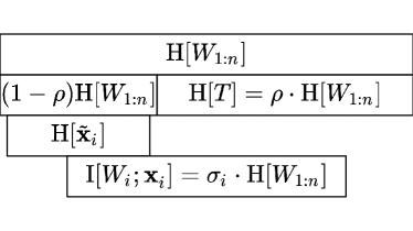
Figure 6: Illustration of Theorem 1.

First of all, look at the entropy $\operatorname{H}[X]$ as the amount of information in the variable $X$. Imagine amounts of information as bars. These bars overlap if there is shared information between the respective variables.

The annotation $T$ and the embedding vector $\tilde{\mathbf{x}}_{i}$ are derived from the underlying text $W_{1:n}$, thus $W_{1:n}$ contains more information than $T$ or $\tilde{\mathbf{x}}_{i}$, hence $\operatorname{H}[W_{1:n}]$ fully covers $\operatorname{H}[T]$ and $\operatorname{H}[\tilde{\mathbf{x}}_{i}]$. Since the mutual information $\operatorname{I}[W_{i};\tilde{\mathbf{x}}_{i}]$ cannot exceed the information in $\tilde{\mathbf{x}}_{i}$, we can write

$$\operatorname{I}[W_{i};\tilde{\mathbf{x}}_{i}]\leq\operatorname{H}[\tilde{\mathbf{x}}_{i}].$$ (4)

Now recall the Eq. (2): it simply means that $\rho$ is the fraction of information that is left in $T$ after it was derived from $W_{1:n}$. This immediately implies that the information which is not in $T$ (but was in $W_{1:n}$ initially) is equal to $(1-\rho)\cdot\operatorname{H}[W_{1:n}]$.

Since the embedding $\tilde{\mathbf{x}}_{i}$ contains no information about the annotation $T$, $\operatorname{H}[\tilde{\mathbf{x}}_{i}]$ and $\operatorname{H}[T]$ do not overlap. But this means that

$$\operatorname{H}[\tilde{\mathbf{x}}_{i}]\leq(1-\rho)\cdot\operatorname{H}[W_{1:n}],$$ (5)

because $\tilde{\mathbf{x}}_{i}$ is in the category of no information about $T$.

Combining (1), (4), (5), and the assumption $\rho>1-\sigma_{i}$, we have

$$\operatorname{I}[W_{i};\tilde{\mathbf{x}}_{i}]\leq(1-\rho)\cdot\operatorname{H}[W_{1:n}]<\sigma_{i}\cdot\operatorname{H}[W_{1:n}]=\operatorname{I}[W_{i};\mathbf{x}_{i}],$$

$$\Rightarrow\quad\operatorname{I}[W_{i};\mathbf{x}_{i}]-\operatorname{I}[W_{i};\tilde{\mathbf{x}}_{i}]>(\rho+\sigma_{i}-1)\cdot\operatorname{H}[W_{1:n}].$$ (6)

The inequality (6) is almost the required (3)—it remains to show that the change in mutual information can be approximated by the change in LM loss; this is done in Lemma E.2. ∎

Role of $\rho$ and $\sigma_{i}$.

Equation (2) quantifies the dependence between $T$ and $W_{1:n}$, and it simply means that the annotation $T$ carries $100\cdot\rho\%$ of information contained in the underlying text $W_{1:n}$ (in the information-theoretic sense). The quantity $\rho$ is well known as the entropy coefficient in the information theory literature (?). It can be thought of as an analog of the correlation coefficient for measuring not only linear or monotonic dependence between numerical variables but any kind of statistical dependence between any kind of variables (numerical and non-numerical). As we see from Equation (3), the coefficient $\rho$ plays a key role in predicting the LM degradation when the linguistic structure $T$ is removed from the embedding $\mathbf{x}_{i}$. In Section 3.3 we give a practical way of its estimation for the case when $T$ is a per-token annotation of $W_{1:n}$.

Similarly, Equation (1) means that both $W_{i}$ and $\mathbf{x}_{i}$ carry at least $100\cdot\sigma_{i}\%$ of information contained in $W_{1:n}$. By Firth’s distributional hypothesis (?), we assume that $\sigma_{i}$ significantly exceeds zero.

Range of $\rho$.

In general, mutual information is non-negative. Mutual information of the annotation $T$ and the underlying text $W_{1:n}$ cannot exceed information contained in either of these variables, i.e. $0\leq\operatorname{I}[T;W_{1:n}]\leq\operatorname{H}[W_{1:n}]$, and therefore $\rho\in[0,1]$.

Absence of information.

When we write “$\tilde{\mathbf{x}}_{i}$ contains no information on $T$”, this means that the mutual information between $\tilde{\mathbf{x}}_{i}$ and $T$ is zero:

$$\operatorname{I}[T;\tilde{\mathbf{x}}_{i}]=0.$$ (7)

In the language of ? (?), Equation (7) assumes that all probes—even the best—perform poorly in extracting $T$ from $\tilde{\mathbf{x}}_{i}$. This essentially means that the information on $T$ has been filtered out of $\tilde{\mathbf{x}}$. In practice, we will approximate this with the techniques of Gradient Reversal Layer (?) and Iterative Nullspace Projection (?).

3.3 Experiments

In this section, we empirically verify the prediction of our theory—the stronger the dependence of a linguistic property with the underlying text the greater the decline in the performance of a language model that does not have access to such property.

Here we will focus on only one contextualized embedding model, BERT because it is the most mainstream model. Along with this, we will keep the SGNS for consideration as a model of static embeddings.

3.3.1 Removal Techniques

We consider two ways of removing linguistic information from the embeddings: Gradient Reversal Layer (GRL) and Iterative Nullspace Projection (INLP).

GRL (?)

is a method of adversarial training that, in our case, can be used to remove linguistic information $T$ from word embeddings $\boldsymbol{\xi}$. For this, the pretraining model is formulated as $\widehat{W}=\omega(\boldsymbol{\xi})$, and an auxiliary model is $\widehat{T}=\tau(\boldsymbol{\xi})$. The training procedure optimizes

$$\min_{\omega,\tau,\boldsymbol{\xi}}\left[\ell(\omega(\boldsymbol{\xi}),W)+\ell(\tau(\gamma_{\lambda}(\boldsymbol{\xi})),T)\right]$$

where $\ell(\cdot,\cdot)$ is the loss function, and $\gamma_{\lambda}$ is a layer inserted between $\boldsymbol{\xi}$ and $\tau$ which acts as the identity during the forward pass, while it scales the gradients passed through it by $-\lambda$ during backpropagation. In theory, the resulting embeddings $\tilde{\mathbf{x}}$ are maximally informative for the pretraining task while at the same time minimally informative for the auxiliary task. However, in practice, GRL not always succeeds to fully remove the auxiliary information from the embeddings as was shown by ? (?) (and confirmed by our experiments in Appendix F).

INLP (?)

is a method of post-hoc removal of some property $T$ from the pretrained embeddings ${\mathbf{x}}$. INLP neutralizes the ability to linearly predict $T$ from $\mathbf{x}$ (here $T$ is a single tag, and $\mathbf{x}$ is a single vector). It does so by training a sequence of auxiliary models $\tau_{1},\ldots,\tau_{k}$ that predict $T$ from $\mathbf{x}$, interpreting each one as conveying information on unique directions in the latent space that correspond to $T$, and iteratively removing each of these directions. In the $i^{\text{th}}$ iteration, $\tau_{i}$ is a linear model parameterized by a matrix $\mathbf{U}_{i}$ and trained to predict $T$ from $\mathbf{x}$. When the embeddings are projected onto $\mathrm{null}(\textbf{U}_{i})$ by a projection matrix $\mathbf{P}_{\mathrm{null}(\mathbf{U}_{i})}$, we have

$$\mathbf{U}_{i}\mathbf{P}_{\mathrm{null}(\mathbf{U}_{i})}\mathbf{x}=\mathbf{0},$$

i.e. $\tau_{i}$ will be unable to predict $T$ from $\mathbf{P}_{\mathrm{null}(\mathbf{U}_{i})}\mathbf{x}$. Figure 7 illustrates the method for the case when the property $T$ has only two types of tags and $\mathbf{x}\in\mathbb{R}^{2}$.

Figure 7: Nullspace projection for a 2-dimensional binary classifier. The decision boundary of $\mathbf{U}_{i}$ is $\mathbf{U}_{i}$’s null-space. Source: ? (?).

The number of iterations $k$ is taken such that no linear classifier achieves above-majority accuracy when predicting $T$ from $\tilde{\mathbf{x}}=\mathbf{P}_{\mathrm{null}(\mathbf{U}_{k})}\mathbf{P}_{\mathrm{null}(\mathbf{U}_{k-1})}\ldots\mathbf{P}_{\mathrm{null}(\mathbf{U}_{1})}\mathbf{x}$. Before measuring the LM loss we allow the model to adapt to the modified embeddings $\tilde{\mathbf{x}}$ by fine-tuning its softmax layer that predicts $W$ from $\tilde{\mathbf{x}}$, while keeping the rest of the model (encoding layers) frozen. This fine-tuning does not bring back information on $T$ as the softmax layer linearly separates classes.

3.3.2 Tasks

We perform experiments on two real tasks and a series of synthetic tasks. In real tasks, we cannot arbitrarily change $\rho$—we can only measure it for some given annotations. Although we have several real annotations that give some variation in the values of $\rho$, we want more control over this metric. Therefore, we come up with synthetic annotations that allow us to smoothly change $\rho$ in a wider range and track the impact on the loss function of a language model.

To remove a property $T$ from embeddings, INLP requires a small annotated dataset, while GRL needs the whole pretraining corpus to be annotated. Therefore for INLP we use gold annotations, while for GRL we tag the pretraining data with the help of the Stanza tagger (?).

Real tasks.

We consider two real tasks with per-token annotations: part-of-speech tagging (POS) and named entity labeling (NER). The choice of per-token annotations is guided by the suggested method of estimating $\rho$ (Section 3.3.3).

POS is the syntactic task of assigning tags such as noun, verb, adjective, etc. to individual tokens. We consider POS tagged datasets that are annotated with different tagsets:

• Universal Dependencies English Web Treebank (UD EWT, ?), which uses two annotation schemas: UPOS corresponding to 17 universal tags across languages, and FPOS which encodes additional lexical and grammatical properties.

• English part of the OntoNotes corpus (?) based on the Penn Treebank annotation schema (?).

NER is the task of predicting the category of an entity referred to by a given token, e.g. does the entity refer to a person, a location, an organization, etc. This task is taken from the English part of the OntoNotes corpus.

Note that the Stanza tagger, used to generate annotations for GRL training, relies on universal tagset from Universal Dependencies (UPOS) for POS tagging, and on OntoNotes NER annotations. Table 2 reports some statistics on the size of different tagsets.

UD UPOS	UD FPOS	ON POS	ON NER
17	50	48	66

Table 2: Size of the tagsets for Universal Dependencies and OntoNotes PoS tagging and NER datasets.

Synthetic tasks

are created as follows. Let $T^{(0)}$ be an annotation of a corpus $W_{1:n}$, which has $m$ unique tags, and let the corresponding $\rho^{(0)}:=\operatorname{I}[T^{(0)};W_{1:n}]/\operatorname{H}[W_{1:n}]$. We select the two least frequent tags from the tagset, and conflate them into one tag. This gives us an annotation $T^{(1)}$ which contains less information about $W_{1:n}$ than the annotation $T^{(0)}$, and thus has $\rho^{(1)}<\rho^{(0)}$. In Table 3 we give an example of such conflation for a POS-tagged sentence from the OntoNotes corpus (?).

$W_{1:9}$	When	a	browser	starts	to	edge	near	to	consuming
$T^{(0)}$	WRB	DT	NN	VBZ	TO	VB	RB	IN	VBG
$T^{(1)}$	X	DT	NN	VBZ	X	VB	RB	IN	VBG
$W_{10:18}$	500	MB	of	RAM	on	a	regular	basis	,
$T^{(0)}$	CD	NNS	IN	NN	IN	DT	JJ	NN	,
$T^{(1)}$	CD	NNS	IN	NN	IN	DT	JJ	NN	,
$W_{19:22}$	something	is	wrong	.
$T^{(0)}$	NN	VBZ	JJ	.
$T^{(1)}$	NN	VBZ	JJ	.

Table 3: Example of conflating two least frequent tags (WRB and TO) into one tag (X).

Next, we select two least frequent tags from the annotation $T^{(1)}$ and conflate them. This will give an annotation $T^{(2)}$ with $\rho^{(2)}<\rho^{(1)}$. Iterating this process $m-1$ times we will end up with the annotation $T^{(m-1)}$ that tags all tokens with a single (most frequent) tag. In this last iteration, the annotation has no mutual information with $W_{1:n}$, i.e. $\rho^{(m-1)}=0$.

3.3.3 Experimental Setup

We remove (pseudo-)linguistic structures (Section 3.3.2) from BERT and SGNS embeddings using the methods from Section 3.3.1, and measure the decline in the language modeling performance. Assuming that $\Delta\ell_{\omega,T,\mu}$ is the validation loss increase of the embedding model $\omega\in\{\textsc{BERT},\textsc{SGNS}\}$ when information on $T\in\{\text{Synthetic},\text{POS},\text{NER}\}$ is removed from $\omega$ using the removal method $\mu\in\{\text{GRL},\text{INLP}\}$, we compare $|\Delta\ell_{\omega,T,\mu}|$ against $\rho$ defined by (2) which is the strength of interdependence between the underlying text $W_{1:n}$ and its annotation $T$. By Theorem 1, $\Delta\ell_{\omega,T,\mu}$ is $\Omega(\rho)$ for any combination of $\omega$, $T$, $\mu$.

Estimating $\rho$.

Recall that $\rho:=\operatorname{I}[T;W_{1:n}]/\operatorname{H}[W_{1:n}]$ (Eq. 2) and that the annotation $T$ is a deterministic function of the underlying text $W_{1:n}$ (Sec. 3.1). In this case, we can write

$$\rho=\frac{\operatorname{H}[T]-\overbrace{\operatorname{H}[T\mid W_{1:n}]}^{0}}{\operatorname{H}[W_{1:n}]}=\frac{\operatorname{H}[T]}{\operatorname{H}[W_{1:n}]}.$$ (8)

and when $T$ is a per-token annotation of $W_{1:n}$, i.e. $T=T_{1:n}$ (which is the case for the annotations that we consider), this becomes $\rho=\operatorname{H}[T_{1:n}]/\operatorname{H}[W_{1:n}]$. Thus to estimate $\rho$, we simply need to be able to estimate the latter two entropies. This can be done by training an autoregressive sequence model, such as LSTM, on $W_{1:n}$ and on $T_{1:n}$. The loss function of such a model—the cross-entropy loss—serves as an estimate of the required entropy. Notice, that we cannot use masked LMs for this estimation as they do not give a proper factorization of the probability $p(w_{1},\ldots,w_{n})$. Thus, we decided to choose the AWD-LSTM-MoS model of ? (?) which is a compact and competitive LM that can be trained in a reasonable time and with moderate computing resources. In addition, we also estimated the entropies through a vanilla LSTM with tied input and output embeddings (?), and a Kneser-Ney 3-gram model (?) to test how strongly our method depends on the underlying sequence model.

Limitations.

The suggested method of estimating $\rho$ through autoregressive sequence models is limited to per-token annotations only. However, according to formula (8), to estimate $\rho$ for deeper annotations, it is sufficient to be able to estimate the entropy $\operatorname{H}[T]$ of such deeper linguistic structures $T$. For example, to estimate the entropy of a parse tree, one can use the cross-entropy produced by a probabilistic parser. The only limitation is the determinism of the annotation process.

Amount of information to remove.

Each of the removal methods has a hyperparameter that controls how much of the linguistic information $T$ is removed from the word vectors $\mathbf{x}$—the number of iterations in INLP and $\lambda$ in GRL. Following ? (?) we keep iterating the INLP procedure or increasing $\lambda$ in GRL until the performance of a linear probe that predicts $T$ from the filtered embeddings $\tilde{\mathbf{x}}$ drops to the majority-class accuracy. When this happens we treat the resulting filtered embeddings $\tilde{\mathbf{x}}$ as containing no information on $T$.

Optimization details.

For the INLP experiments we use pretrained BERT-Base from HuggingFace (?), and an SGNS pretrained in-house (?). For the GRL experiments we pretrain LMs ourselves, details are in Appendix A.

3.3.4 Results

Real tasks.

Table 4 reports the loss drop of pretrained LM when removing linguistic information (POS or NER) from the pretrained model. Plots that illustrate how losses and probing accuracies change with INLP iterations are provided in Appendix G.

First, we compare UPOS tagsets versus FPOS tagset: intuitively FPOS should have a tighter link with underlying text, and therefore result in higher $\rho$ and as a consequence in a higher drop in loss after the removal of this information from words representations. This is confirmed by the numbers reported in Table 4.

We also see a greater LM performance drop when the POS information is removed from the models compared to NE information removal. This is in line with Theorem 1 as POS tags depend stronger on the underlying text than NE labels as measured by $\rho$.

In the case of pretraining SGNS with GRL, we could not reach the majority class accuracy. Reported is the loss increase for the model that had the lowest accuracy ($\text{Acc}=.466$ while the majority accuracy for this task is $.126$). If it were possible to train the SGNS model with GRL removing POS tags and reaching the majority class accuracy, its loss increase would be even higher than the one reported.

Removal method $\mu$	INLP				GRL
Annotation $T$	ON NER	UD UPOS	UD FPOS	ON POS	NER	UPOS
$\rho$ (AWD-LSTM-MoS)	0.18	0.32	0.36	0.42	0.18	0.43
$\rho$ (LSTM)	0.18	0.32	0.37	0.42	0.22	0.34
$\rho$ (KN-3)	0.18	0.36	0.41	0.42	0.17	0.37
$\Delta\ell_{\textsc{BERT},T,\mu}$	0.13	0.54	0.70	0.87	6.16	6.16
$\Delta\ell_{\textsc{SGNS},T,\mu}$	1.33	1.62	1.79	2.04	0.32	$>$1.1†

Table 4: Results on POS tagging and NER tasks. ON stands for OntoNotes, UD for Universal Dependencies. The UD EWT dataset has two types of POS annotation: coarse tags (UPOS) and fine-grained tags (FPOS). ^†GRL for SGNS on UPOS annotation did not reach the majority class accuracy (.126). KN-3 is a Kneser-Ney 3-gram model.

We note larger $\Delta\ell_{\text{\sc BERT},T,\text{GRL}}$ compared to $\Delta\ell_{\text{\sc BERT},T,\text{INLP}}$. We attribute it to the following: INLP works with already pretrained optimal $\omega$ and we fine-tune its softmax layer for modified embeddings $\tilde{\mathbf{x}}$, while GRL with a large $\lambda$ (that is needed to bring the probing accuracy down to a majority class) moves $\omega$’s weights into a bad local minimum when pretraining from scratch. Moreover, the pretrained BERT from HuggingFace and RoBERTa pretrained by us are pretrained over different corpora and are using different vocabularies. Thus increases in the cross-entropies caused by INLP and by GRL are not directly comparable.

We attempted to conduct experiments on GRL in such a way that their results were comparable to the results of the INLP—we tried to fine-tune a pretrained RoBERTa with GRL. However, our attempt was not successful as we did not manage to reach majority class accuracy (more details in Appendix F). This reinforces ?’s (?) argument that GRL has more difficulties removing fully the auxiliary information from the word representations.

Finally, we see that although $\rho$ indeed depends on the underlying sequence model that is used to estimate the entropies $\operatorname{H}[T_{1:n}]$ and $\operatorname{H}[W_{1:n}]$, all models—AWD-LSTM-MoS, LSTM, and KN-3—preserve the relative order for the annotations that we consider. E.g., all models indicate that OntoNotes NER annotation is the least interdependent with the underlying text, while OntoNotes POS annotation is the most interdependent one. In addition, it turns out that for a quick estimate of $\rho$, one can use the KN-3 model, which on a modern laptop calculates the entropy of texts of 100 million tokens in a few minutes, in contrast to the LSTM, which takes several hours on a modern GPU.

Synthetic tasks.

To obtain synthetic data, we apply the procedure described in Sect. 3.3.2 to the OntoNotes POS annotation as it has the highest $\rho$ in Table 4 and thus allows us to vary the metric in a wider range.

The results of evaluation on the synthetic tasks through the INLP are provided in Figure 8.

Figure 8: Synthetic task results for INLP. $\Delta\ell$ is the increase in cross-entropy loss when pseudo-linguistic information is removed from the BERT’s last layer with the INLP procedure. $\rho$ is estimated with the help of AWD-LSTM-MoS model (?) as described in Section 3.3.3.

They validate the predictions of our theory—for the annotations with greater $\rho$ there is a bigger drop in the LM performance (i.e. increase in the LM loss) when the information on such annotations is removed from the embeddings. We notice that $\Delta\ell$ is piecewise-linear in $\rho$ with the slope changing at $\rho\approx 0.4$. We attribute this change to the following: for $\rho<0.4$, the majority class (i.e. the most frequent tag) is the tag that encapsulates several conflated tags (see Subsection 3.3.2 for details), while for $\rho>0.4$, the majority is NN tag. This switch causes a significant drop in the majority class accuracy which in turn causes a significant increase in the number of INLP iterations to reach that accuracy, and hence an increase in the amount of information being removed which implies greater degradation of the LM performance.

4 Related Work

Theoretical analysis.

Since the success of early word embedding algorithms like SGNS and GloVe, there were attempts to analyze theoretically the connection between their pretraining objectives and performance on downstream tasks such as word similarity and word analogy tasks. An incomplete list of such attempts includes those of ? (?, ?, ?, ?, ?, ?, ?). Most of these works represent pretraining as a low-rank approximation of some co-occurrence matrix—such as PMI—and then use an empirical fact that the set of columns (or rows) of such a matrix is already a good solution to the analogy and similarity tasks. Recently, we have seen a growing number of works devoted to the theoretical analysis of contextualized embeddings. ? (?) showed that modern embedding models, as well as the old warrior SGNS, maximize an objective function that is a lower bound on the mutual information between different parts of the text. ? (?) formalized how solving certain pretraining tasks allows learning representations that provably decrease the sample complexity of downstream supervised tasks. Of particular interest is a recent paper by ? (?) that relates a pretraining performance of an autoregressive LM with a downstream performance for downstream tasks that can be reformulated as next word prediction tasks. The authors showed that for such tasks, if the pretraining objective is $\epsilon$-optimal, then the downstream objective of a linear classifier is $\mathcal{O}(\sqrt{\epsilon})$-optimal. In the second part of our work (Section 3) we prove a similar statement, but the difference is that we study how the removal of linguistic information affects the pretraining objective and our approach is not limited to downstream tasks that can be reformulated as next word prediction.

Probing.

Early work on probing tried to analyze LSTM language models (?, ?, ?, ?, ?, ?, ?). Moreover, word similarity (?) and word analogy (?) tasks can be regarded as non-parametric probes of static embeddings such as SGNS (?) and GloVe (?). Recently the probing approach has been used mainly for the analysis of contextualized word embeddings. ? (?) for example showed that entire parse trees can be linearly extracted from ELMo’s (?) and BERT’s (?) hidden layers. ? (?) probed contextualized embeddings for various linguistic phenomena and showed that, in general, contextualized embeddings improve over their non-contextualized counterparts largely on syntactic tasks (e.g., constituent labeling) in comparison to semantic tasks (e.g., coreference). The probing methodology has also shown that BERT learns some reflections of semantics (?) and factual knowledge (?) into the linguistic form which are useful in applications such as word sense disambiguation and question answering respectively. ? (?) analyzed how the quality of representations in a pretrained model evolves with the amount of pretraining data. They performed extensive probing experiments on various NLU tasks and found that pretraining with 10M sentences was already able to solve most of the syntactic tasks, while it required 1B training sentences to be able to solve tasks requiring semantic knowledge (such as Named Entity Labeling, Semantic Role Labeling, and some others as defined by ? (?)).

Closest to our second part (Section 3), ? (?) propose to look at probing from a different angle, proposing amnesic probing which is defined as the drop in performance of a pretrained LM after the relevant linguistic information is removed from one of its layers. The notion of amnesic probing fully relies on the assumption that the amount of the linguistic information contained in the pretrained vectors should correlate with the drop in LM performance after this information is removed. In this work (Section 3) we theoretically prove this assumption. While ? (?) measured LM performance as word prediction accuracy, we focus on the native LM cross-entropy loss. In addition, we answer one of the questions raised by the authors on how to measure the influence of different linguistic properties on the word prediction task—we provide an easy-to-estimate metric that does exactly this.

Criticism of probing.

The probing approach has been criticized from different angles. Our attempt to systematize this line of work is given in Figure 9.

Figure 9: Criticism and improvement of the probing methodology. An arrow $A\to B$ means that $B$ criticizes and/or improves $A$.

The seminal paper of ? (?) raises the issue of separation between extracting linguistic structures from contextualized embeddings and learning such structures by the probes themselves. This dichotomy was challenged by ? (?, ?), but later validated by ? (?) using an information-theoretic view on probing. Meanwhile, methods were proposed that take into account not only the probing performance but also the ease of extracting linguistic information (?) or the complexity of the probing model (?). At the same time, ? (?) and ? (?) suggested avoiding learnability issues by non-parametric probing and weak supervision respectively. The remainder of the criticism is directed at the limitations of probing such as insufficient reliability for low-resourced languages (?), lack of evidence that probes indeed extract linguistic structures but do not learn from the linear context only (?), lack of correlation with fine-tuning scores (?) and with pretraining scores (?, ?). The first part of our work (Section 2) partly falls into this latter group, as we did not find any evidence for a correlation between probing scores and pretraining objectives for better performing CoVe (?).

Pruning language models.

A recent work by ? (?) compressed BERT using conventional pruning and showed a linear correlation between pretraining loss and downstream task accuracy. ? (?) pruned pretrained BERT with LTH and fine-tuned it to downstream tasks, while ? (?) pruned fine-tuned BERT with LTH and then re-fine-tuned it. ? (?) showed that the weights needed for specific tasks are a small subset of the weights needed for masked language modeling, but they prune during fine-tuning which is beyond the scope of our work. ? (?) propose to learn the masks of the pretrained LM as an alternative to finetuning on downstream tasks and shows that it is possible to find a subnetwork of large pretrained model which can reach the performance on the downstream tasks comparable to finetuning on this task. Generally speaking, the findings of the above-mentioned papers are aligned with our findings that the performance of pruned models on downstream tasks is correlated with the pretraining loss. The one difference from Section 2 of our work is that most of the previous work looks at the performance of fine-tuned pruned models. In our work, we probe pruned models, i.e. the remaining weights of language models are not adjusted to the downstream probing task. It is not obvious whether the conclusions from the former should carry over to the latter.

5 Conclusion

In this work, we tried to better understand the phenomenon of the rediscovery hypothesis in pretrained language models. Our main contribution is two-fold: we demonstrate that the rediscovery hypothesis

• holds across various pretrained LMs (SGNS, CoVE, RoBERTa) even when a significant amount of weights get pruned (in English);

• can be formally defined within an information-theoretic framework and proved (assuming that the linguistic annotation is a deterministic function of the underlying text and that the annotation is sufficiently interdependent with the text).

First (Section 2), we performed probing of different pruned instances of the original models. If models are overparametrized, then it could be that the pruned model only keeps the connections that are important for the pretraining task, but not for auxiliary tasks like probing. Our experiments show that there is a correlation between the pretrained model’s cross-entropy loss and probing performance on various linguistic tasks. We believe that such correlation can be interpreted as strong evidence in favor of the rediscovery hypothesis.

While performing the above-mentioned analysis, several additional interesting observations have been made.

• Break-down frequency analysis (Section 2.5) reveals that at moderate pruning rates the POS tag performance drop is quite similar across all the token frequency groups. It indicates that to preserve LM performance, the pruned models were forced to distribute their “linguistic knowledge” across all the token groups, and thus reinforces the rediscovery hypothesis.

  We noted, however, that part of the probing performance could be due to exploitation of spurious memorization in pretraining LM. A question on whether such spurious memorization should be considered as linguistic knowledge learnt by pretrained LM is an ongoing debate in the community (?, ?). We believe that further investigation in this direction could bring more insights into the pretrained model’s behavior.

• We have analyzed how the amount of linguistic knowledge evolves during the pretraining process. Our analysis of intermediate pretraining checkpoints suggests that models follow NLP pipeline discovery during the pretraining process: it reaches good performance on syntactic tasks at the beginning of the training and keeps improving on semantic tasks further in training.

Section 3 proposes an information-theoretic formulation of the rediscovery hypothesis and a measure of the dependence between the text and linguistic annotations. In particular, Theorem 1 states that neural language models do need to discover linguistic information to perform at their best: when the language models are denied access to linguistic information, their performance is not optimal. The metric $\rho$, which naturally appears in the development of our information-theoretic framework proposes a measure of the relationship between a given linguistic property and the underlying text. We show that it is also a reliable predictor of how suboptimal a language model will be if it is denied access to a given linguistic property. Our proposed methods of estimating $\rho$ can be used in further studies to quantify the dependence between text and its per-token annotation.

A number of previous studies (?, ?, ?, ?) have shown some evidence in favour of rediscovery hypothesis, while many others (?, ?, ?, ?) questioned the methodology of those studies. However, none of the above-mentioned works questioned the rediscovery hypothesis per se nor demonstrated any evidence for rejecting it. We believe that our work brings an additional understanding of this phenomenon. In addition, it is the first attempt to formalize the rediscovery hypothesis and provide a theoretical frame for it.

A Optimization

CoVe

Two-layer BiLSTM encoder with size 600. For embedding matrix, we use GloVe embeddings with 840B tokens and fix embedding matrix while training as was done in the original implementation (?). Thus we do not prune the embedding matrix in LTH experiments. For training, we used IWSLT 16 dataset. Scripts for preprocessing the data and training the model were adapted to a newer version of OpenNMT-py (?). We use the default hyperparameters of OpenNMT-py: batch size 64, maximum training steps 100,000. We use the following early stopping criterion: we stop training the model if there is no improvement in 3 consecutive validation perplexity scores (validation is performed every 2,000 steps).

RoBERTa

Optimization is performed on the full Wikitext-103 data. We used the default roberta.base tokenizer (distributed along with roberta.base model) (?). The following training settings were used for training on 2 GPUs for 100 epochs:

• architecture: embedding size 512, 6 layers, 4 heads, hidden size 1024

• batch size: 4096 tokens (with gradient accumulation for 4 steps)

• dropout 0.3

Pruning rates used for LTH experiments are chosen as follows:

• step $0.025$ for pruning up to 20% of model parameters

• step $0.05$ between 20% until 70% of model parameters

SGNS

Embedding size 200, 15 epochs to train, 5 negative samples per training example, batch size 1024, window size 5. For training we use the text8 dataset (?), which is the first 100MB of the English Wikipedia dump on Mar. 3, 2006. For validation we use the next 10MB of the same dump. We were ignoring words that appeared less than 5 times in text8, and subsampling the rest as follows: each word $w$ in training set is discarded with probability $p=\sqrt{t/f(w)}+t/f(w)$, where $t=10^{-4}$, and $f(w)$ is the frequency of word $w$. We use Adam optimizer with its default settings.

B Lack of Correlation for Better Performing Models

In Section 2 we noticed that when restricting the loss values of CoVe to the better performing end (zoomed in regions in Figure 10), drop in probing scores (compared to the scores of the baseline unpruned model) become indistinguishable. Here we treat this claim more rigorously. Assuming that $\ell^{\textsc{CoVe}}_{i}$ is the validation loss of CoVe at iteration $i$, and $\Delta s^{\textsc{CoVe},T}_{i}$ is the corresponding drop in the score on the probing task $T\in\{$NE, POS, Constituents, Structural$\}$, we obtain pairs $(\ell^{{\textsc{CoVe}}}_{i},\Delta s^{{\textsc{CoVe}},{T}}_{i})$ and setup a simple linear regression for the zoomed in regions in Figure 10:

Figure 10: Zooming in on better performing CoVe models. Indication of the region to be zoomed in (left) and the zoomed in region (right).

$$\Delta s^{\textsc{CoVe},T}_{i}=\alpha+\beta\cdot\ell^{\textsc{CoVe}}_{i}+\epsilon_{i}.$$

Below are $p$-values when testing $H_{0}:\,\beta=0$ with a two-sided Student $t$-test.

Task	NE	POS	Constituents	Structural
p-value	0.725	0.306	0.184	0.160

Table 5: Testing $\beta=0$, reported are $p$-values.

In all cases $\beta$ is not significantly different from $0$. Hence, the correlation between model performance and its linguistic knowledge may become very weak for better solutions to the pretraining objectives. We argue that this phenomenon is related to the amount of information remaining in an LM after pruning, and how much of this information is enough for the probe. It turns out that in the best CoVe (with the lowest pretraining loss) such information is redundant for the probe, and in the not-so-good (but still decent) CoVe there is just enough of information for the probe to show its best performance.

MDL Analysis

Recently, ? (?) have addressed a related issue by proposing a minimum description length (MDL) analysis of probes, that takes into account the difficulty of extracting the information. Here, we apply their analysis to CoVe (that is faster to experiment with than RoBERTA), on top of the edge probe for constituents. The resulting online codelengths vs cross-entropy values are provided in Fig. 12.

Figure 11: MDL probing of CoVe for constituents (online code). Unlike F1 score, the codelength takes into account not only the performance but also the amount of efforts to achieve it.

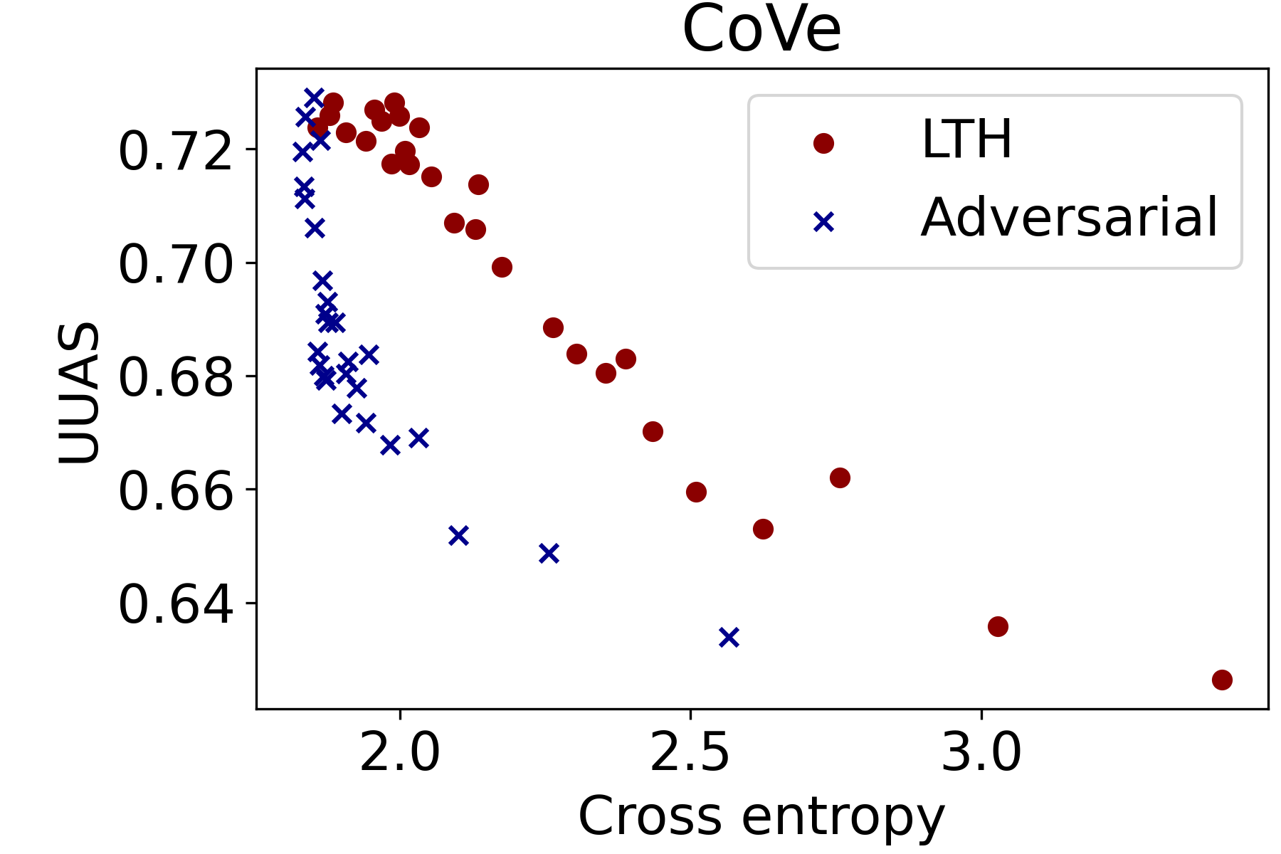
Figure 12: Structural probing of adversarially trained CoVe.

We observe an even wider spectrum of models (with cross-entropies 1.9–2.5) that have indistinguishable codelengths. Nevertheless, the overall pattern does not contradict the rediscovery hypothesis—better models have better probing scores (lower codelengths).

C Adversarial Training

In Sect. 2.3 we have analyzed linguistic knowledge discovered through standard language modeling pretraining. Here we propose a more radical approach, consisting in explicitly adding adversarial noise to the pretraining objective of CoVe that enforces random angles between contextualized representations of nearby words in the source sentence of the translation task. Different to what is done in Sect. 3, this is done on CoVE. For this, we exploit an empirical fact that the cosine similarity between word vectors tends to be a good predictor of their semantic similarity when trained non-adversarially. We vary the amount of noise (through a hyperparameter), train the models, and probe them with the structural probe.

C.1 Training Details

Let $F=[f_{1},f_{2},\ldots,f_{n}]$ be a sentence in the source language, and $E=[e_{1},e_{2},\ldots,e_{m}]$ be a corresponding sentence in the target language. Parallel corpus is the set of sentence pairs $\mathcal{D}=\{(F,E)\}$. Neural machine translation (NMT) model parameterized by $\boldsymbol{\theta}$ solves

$$\min_{\boldsymbol{\theta}}\frac{1}{|\mathcal{D}|}\sum_{(F,E)\in\mathcal{D}}\underbrace{-\log p_{\boldsymbol{\theta}}(E\mid F)}_{\ell^{\text{NMT}}(F,E)}$$ (9)

In case of CoVE, the NMT model is an LSTM-based encoder-decoder architecture with attention (?), and let $\mathbf{h}_{1:n}=[\mathbf{h}_{1},\mathbf{h}_{2},\ldots,\mathbf{h}_{n}]$ be the top-level activations of the encoder that correspond to the sentence $F$.

Recall that for a pair of words $f_{i}$ and $f_{j}$, the cosine similarity between their vector representations $\mathbf{h}_{i}$ and $\mathbf{h}_{j}$ strongly correlates with the human similarity rating $r(f_{i},f_{j})$ (?). Strong correlation means that there is an approximately linear relationship between $r(f_{i},f_{j})$ and $\cos(\mathbf{h}_{i},\mathbf{h}_{j})$. In order to “break” this relationship we fit $\cos(\mathbf{h}_{i},\mathbf{h}_{j})$ to a random $r\sim\mathcal{U}(0,1)$ for nearby source words while training the NMT model (which CoVe model is based on). For a pair $(F,E)$ an individual objective becomes

$$\ell(F,E)=\ell^{\text{NMT}}(F,E)+\alpha\cdot\ell^{\text{Adv}}(F),$$

where

$$\ell^{\text{Adv}}(F)=\frac{1}{n}\sum_{i=1+k}^{n-k}\sum_{\begin{subarray}{c}i-k\leq j\leq i+k\\ j\neq 0\end{subarray}}\mathbb{E}_{r_{ij}\sim\mathcal{U}(0,1)}[w\cdot\cos(\mathbf{h}_{i},\mathbf{h}_{j})+b-r_{ij}]^{2},$$

$w$ and $b$ are regression coefficients, $k$ is the size of a sliding window, in our experiments we use $k=5$. Hyperparameter $\alpha$ regulates the impact of the adversarial loss.

C.2 Results

The probing results are provided in Fig. 12, where cross entropies are CoVe’s validation loss values without the adversarial additive. Although the probing score decreases with an increase of cross-entropy, it does so significantly faster than in the case of LTH—we can have a near-to-best LM with a mediocre probing score. This would suggest that it is possible to find the state of the network that would encode less linguistic information given the same pretraining loss. This is however not the path naturally chosen by the pretraining models, therefore probably more difficult to reach. Note, that several artifacts of CoVE training could also explain these results. First, it can be because the pretrained embedding layer is not updated in these experiments, therefore keeping a good (static) representation of tokens. Moreover, recall that CoVE is an encoder-decoder architecture, and reported cross-entropy loss is computed based on the decoder representations. The adversarial loss however has been defined on the encoder representations. Thus, even if the encoder representations got corrupted, the decoder still has a chance to recover and obtain reasonable cross-entropy loss. More extensive adversarial experiments might be necessary to be able to make any conclusion from this experiment.

D Information Theory Background

For a random variable $X$ with the distribution function $p(x)$, its entropy is defined as

$$\operatorname{H}[X]:=\operatorname{\mathbb{E}}_{X}[-\log p(X)].$$

The quantity inside the expectation, $-\log p(x)$, is usually referred to as information content or surprisal, and can be interpreted as quantifying the level of “surprise” of a particular outcome $x$. As $p(x)\to 0$, the surprise of observing $x$ approaches $+\infty$, and conversely as $p(x)\to 1$, the surprise of observing $x$ approaches $0$. Then the entropy $\operatorname{H}[X]$ can be interpreted as the average level of “information” or “surprise” inherent in the $X$’s possible outcomes. We will use the following

Property D.1.

If $Y=f(X)$, then

$$\operatorname{H}[Y]\leq\operatorname{H}[X],$$ (10)

i.e. the entropy of a variable can only decrease when the latter is passed through a (deterministic) function.

Now let $X$ and $Y$ be a pair of random variables with the joint distribution function $p(x,y)$. The conditional entropy of $Y$ given $X$ is defined as

$$\operatorname{H}[Y\mid X]:=\operatorname{\mathbb{E}}_{X,Y}[-\log p(Y\mid X)],$$

and can be interepreted as the amount of information needed to describe the outcome of $Y$ given that the outcome of $X$ is known. The following property is important for us.

Property D.2.

$\operatorname{H}[Y\mid X]=0\,\,\Leftrightarrow\,\,Y=f(X)$.

The mutual information of $X$ and $Y$ is defined as

$$\operatorname{I}[X;Y]:=\mathbb{E}_{X,Y}\left[\log\frac{p(X,Y)}{p(X)\cdot p(Y)}\right]$$

and is a measure of mutual dependence between $X$ and $Y$. We will need the following properties of the mutual information.

Property D.3.

1. $\operatorname{I}[X;Y]=\operatorname{H}[X]-\operatorname{H}[X\mid Y]=\operatorname{H}[Y]-\operatorname{H}[Y\mid X]$.

2. $\operatorname{I}[X;Y]=0\,\,\Leftrightarrow\,$ $X$ and $Y$ are independent.

3. For a function $f$, $\operatorname{I}[X;Y]\geq\operatorname{I}[X;f(Y)]$.

4. $\operatorname{H}[X,Y]=\operatorname{H}[X]+\operatorname{H}[Y]-\operatorname{I}[X;Y]$,

Property D.3.3 is known as data processing inequality, and it means that post-processing cannot increase information. By post-processing we mean a transformation $f(Y)$ of a random variable $Y$, independent of other random variables. In Property D.3.4, $\operatorname{H}[X,Y]$ is the joint entropy of $X$ and $Y$ which is defined as

$$\operatorname{H}[X,Y]:=\operatorname{\mathbb{E}}_{X,Y}[-\log p(X,Y)]$$

and is a measure of “information” associated with the outcomes of the tuple $(X,Y)$.

E Proof of Theorem 1

The proof is split into two steps: first, in Lemma E.1 we show that the decrease in mutual information $\Delta\operatorname{I}:=\operatorname{I}[W_{i};\mathbf{x}_{i}]-\operatorname{I}[W_{i};\tilde{\mathbf{x}}_{i}]$ is $\Omega(\rho)$, and then in Lemma E.2 we approximate $\Delta\operatorname{I}$ by the increase in cross-entropy loss $\ell(W_{i},\tilde{\mathbf{x}}_{i})-\ell(W_{i},\mathbf{x}_{i})$.

Lemma E.1.

Let $T$ be an annotation of a sentence $W_{1:n}=[W_{1},\ldots,W_{i},\ldots,W_{n}]$ and let $\mathbf{x}_{i}$, $\tilde{\mathbf{x}}_{i}$ be (contextualized) word vectors corresponding to a token $W_{i}$ such that

$$\operatorname{I}[T;\tilde{\mathbf{x}}_{i}]=0.$$ (11)

Denote

$$\rho :=\operatorname{I}[T;W_{1:n}]/\operatorname{H}[W_{1:n}],\quad\rho\in[0,1],$$ (12)

$$\sigma_{i} :=\operatorname{I}[W_{i};\mathbf{x}_{i}]/\operatorname{H}[W_{1:n}],\quad\sigma_{i}\in[0,1].$$ (13)

If $\rho>1-\sigma_{i}$, then

$$\operatorname{I}[W_{i};\tilde{\mathbf{x}}_{i}]<\operatorname{I}[W_{i};\mathbf{x}_{i}].$$ (14)

and the difference $\Delta\operatorname{I}:=\operatorname{I}[W_{i};\mathbf{x}_{i}]-\operatorname{I}[W_{i};\tilde{\mathbf{x}}_{i}]$ is lowerbounded as

$$\Delta\operatorname{I}\geq(\rho+\sigma_{i}-1)\cdot\operatorname{H}[W_{1:n}].$$ (15)

Proof.

From (11) and by Property D.3.4, we have

$$\operatorname{H}[T,\tilde{\mathbf{x}}_{i}] =\operatorname{H}[T]+\operatorname{H}[\tilde{\mathbf{x}}_{i}]-\underbrace{\operatorname{I}[T;\tilde{\mathbf{x}}_{i}]}_{0}$$

$$=\operatorname{H}[T]+\operatorname{H}[\tilde{\mathbf{x}}_{i}].$$ (16)

On the other hand, both the annotation $T$ and the word vectors $\tilde{\mathbf{x}}_{i}$ are obtained from the underlying sentence $W_{1:n}$, and therefore $T=T(W_{1:n})$ and $\tilde{\mathbf{x}}_{i}=\tilde{\mathbf{x}}_{i}(W_{1:n})$, i.e. the tuple $(T,\tilde{\mathbf{x}}_{i})$ is a function of $W_{1:n}$, and by Property D.1,

$$\operatorname{H}[T,\tilde{\mathbf{x}}_{i}]\leq\operatorname{H}[W_{1:n}].$$ (17)

From (16) and (17), we get

$$\operatorname{H}[T]+\operatorname{H}[\tilde{\mathbf{x}}_{i}]\leq\operatorname{H}[W_{1:n}].$$ (18)

Since $T=T(W_{1:n})$ and $\tilde{\mathbf{x}}_{i}=\tilde{\mathbf{x}}_{i}(W_{1:n})$, by Property D.2 we have $\operatorname{H}[T\mid W_{1:n}]=0$ and $\operatorname{H}[\tilde{\mathbf{x}}_{i}\mid W_{1:n}]=0$, and therefore

$$\operatorname{I}[T;W_{1:n}]=\operatorname{H}[T]-\operatorname{H}[T\mid W_{1:n}]=\operatorname{H}[T]$$

Plugging this into (18), rearranging the terms, and taking into account (12), we get

$$\operatorname{H}[\tilde{\mathbf{x}}_{i}]\leq\operatorname{H}[W_{1:n}]-\underbrace{\operatorname{I}[T;W_{1:n}]}_{\rho\cdot\operatorname{H}[W_{1:n}]}=(1-\rho)\cdot\operatorname{H}[W_{1:n}].$$ (19)

Also, by Property D.3.1,

$$\operatorname{I}[W_{i};\tilde{\mathbf{x}}_{i}]=\operatorname{H}[\tilde{\mathbf{x}}_{i}]-\underbrace{\operatorname{H}[\tilde{\mathbf{x}}_{i}\mid W_{i}]}_{\geq 0}\leq\operatorname{H}[\tilde{\mathbf{x}}_{i}]$$ (20)

From (13), (19), (20), and the assumption $\rho>1-\sigma_{i}$, we have

$$\operatorname{I}[W_{i};\tilde{\mathbf{x}}_{i}]\leq\operatorname{H}[\tilde{\mathbf{x}}_{i}]\leq(1-\rho)\cdot\operatorname{H}[W_{1:n}]<\sigma_{i}\cdot\operatorname{H}[W_{1:n}]=\operatorname{I}[W_{i};\mathbf{x}_{i}],$$

which implies (14) and (15).∎

Remark 1.

Equation (12) quantifies the dependence between $T$ and $W_{1:n}$, and it means that $T$ carries $100\cdot\rho\%$ of information contained in $W_{1:n}$. Similarly, Equation (13) means that both $W_{i}$ and $\mathbf{x}_{i}$ carry at least $100\cdot\sigma_{i}\%$ of information contained in $W_{1:n}$. By Firth’s distributional hypothesis (?), $\sigma_{i}$ significantly exceeds zero.

Remark 2.

The mutual information $\operatorname{I}[W_{i};\boldsymbol{\xi}_{i}]$ can be interpreted as the performance of the best language model that tries to predict the token $W_{i}$ given its contextual representation $\boldsymbol{\xi}_{i}$. Therefore, inequalities (14) and (15) mean that removing a linguistic structure from word vectors does harm the performance of a language model based on such word vectors, and the more the linguistic structure is interdependent with the underlying text (that is being predicted by the language model) the bigger is the harm.

We treat $\operatorname{I}[W;\boldsymbol{\xi}]$ as the performance of a language model. However, in practice, this performance is measured by the validation loss $\ell$ of such a model, which is usually the cross-entropy loss. Nevertheless, the change in mutual information can be estimated by the change in the LM objective, as we show below.

Lemma E.2.

Let $\mathbf{x}_{i}$ and $\tilde{\mathbf{x}}_{i}$ be (contextualized) embeddings of a token $W_{i}$ in a sentence $W_{1:n}=[W_{1},\ldots,W_{i},\ldots,W_{n}]$. Let $\ell(W_{i},\boldsymbol{\xi}_{i})$ be the cross-entropy loss of a neural (masked) language model $q_{\boldsymbol{\theta}}(w_{i}\mid\boldsymbol{\xi}_{i})$, parameterized by $\boldsymbol{\theta}$, that provides distribution over the vocabulary $\mathcal{W}$ given vector representation $\boldsymbol{\xi}_{i}$ of the $W_{i}$’s context. Then

$$\operatorname{I}[W_{i};\mathbf{x}_{i}]-\operatorname{I}[W_{i};\tilde{\mathbf{x}}_{i}]\approx\ell(W_{i},\tilde{\mathbf{x}}_{i})-\ell(W_{i},\mathbf{x}_{i}).$$ (21)

Proof.

By Property D.3.1, we have

$$\Delta\operatorname{I}: =\operatorname{I}[W_{i};\mathbf{x}_{i}]-\operatorname{I}[W_{i};\tilde{\mathbf{x}}_{i}]=\operatorname{H}[W_{i}]-\operatorname{H}[W_{i}\mid\mathbf{x}_{i}]-\operatorname{H}[W_{i}]+\operatorname{H}[W_{i}\mid\tilde{\mathbf{x}}_{i}]$$

$$=\operatorname{H}[W_{i}\mid\tilde{\mathbf{x}}_{i}]-\operatorname{H}[W_{i}\mid\mathbf{x}_{i}]\approx\operatorname{H}_{q}[W_{i}\mid\tilde{\mathbf{x}}_{i}]-\operatorname{H}_{q}[W_{i}\mid\mathbf{x}_{i}],$$ (22)

where $\operatorname{H}_{q}[W_{i}\mid\boldsymbol{\xi}_{i}]$—a cross entropy—is an estimate of $\operatorname{H}[W_{i}\mid\boldsymbol{\xi}_{i}]$ when the true distribution $p(w_{i}\mid\boldsymbol{\xi}_{i})$ is replaced by a parametric language model $q_{\boldsymbol{\theta}}(w_{i}\mid\boldsymbol{\xi}_{i})$, which is exactly the cross-entropy loss function of a LM $q$:

$$\operatorname{H}_{q}[W_{i}\mid\boldsymbol{\xi}_{i}]=\operatorname{\mathbb{E}}_{(W_{i},C_{i})\sim\mathcal{D}}[-\log q_{\boldsymbol{\theta}}\left(W_{i}\mid\boldsymbol{\xi}_{i}\right)]=:\ell(W_{i},\boldsymbol{\xi}_{i}).$$ (23)

From (22) and (23), we have (21). ∎

Remark 3.

When we approximate $\operatorname{H}[W_{i}\mid\mathbf{x}_{i}]\approx\mathrm{H}_{q}[W_{i}\mid\mathbf{x}_{i}]$, here the parameters $\boldsymbol{\theta}$ of $q=q_{\boldsymbol{\theta}}(w_{i}\mid\mathbf{x}_{i})$ are only the LM head’s parameters (e.g., the weights and biases of the output softmax layer in BERT), and we assume that $\mathbf{x}_{i}$ can be any representation (e.g., from the last encoding layer of BERT). We assume that $\boldsymbol{\theta}$ are chosen to minimize the KL-divergence between the true distribution $p(w_{i}\mid\mathbf{x}_{i})$ and the model $q_{\boldsymbol{\theta}}(w_{i}\mid\mathbf{x}_{i})$, thus making the approximation reasonable.

Similarly, when we approximate $\operatorname{H}[W_{i}\mid\tilde{\mathbf{x}}_{i}]\approx\operatorname{H}_{q}[W_{i}\mid\tilde{\mathbf{x}}_{i}]$ we again have the LM head $q_{\boldsymbol{\eta}}(w_{i}\mid\tilde{\mathbf{x}}_{i})$, whose parameters $\boldsymbol{\eta}$ should be chosen to minimize the KL-divergence between true $p(w_{i}\mid\tilde{\mathbf{x}}_{i})$ and the model $q_{\boldsymbol{\eta}}(w_{i}\mid\tilde{\mathbf{x}}_{i})$, for the approximation to be reasonable. In the experimental part (Section 3.3), we do exactly this: after applying INLP (or GRL) to a representation, we fine-tune the softmax layer (but keep the encoding layers frozen) so that it can adapt to the modified representation.

F Using GRL in Finetuning Mode

In order to make GRL experiments more comparable to INLP we pretrain BERT (as RoBERTa) on WikiText-103 and finetune it with GRL on the OntoNotes POS annotation The results for different values of the GRL’s $\lambda$ are given in Table 6.

$\lambda$	$\ell_{\text{\sc BERT}}$	Accuracy	$\lambda$	$\ell_{\text{\sc BERT}}$	Accuracy
0	2.062	0.942	10	5.808	0.880
0.1	2.070	0.920	50	6.362	0.844
1	2.647	0.917	100	6.473	0.828
5	3.585	0.913	1000	6.267	0.865

Table 6: Finetuning RoBERTa with GRL on OntoNotes POS annotation.

The majority class accuracy on this dataset is 0.126, and we see that no matter how large the $\lambda$ we take, the GRL still cannot lower the accuracy to this level. This confirms observations of ? (?) that GRL may not always remove all the information from a model it is applied to.

G INLP Dynamics

Figure 13: Loss increase w.r.t. INLP iteration for different tasks. ON stands for OntoNotes, UD for Universal Dependencies. The UD EWT dataset has two types of POS annotation: coarse tags (UPOS) and fine-grained tags (FPOS)

Figure 14: INLP Dynamics for SGNS. ON stands for OntoNotes, UD for Universal Dependencies. The UD EWT dataset has two types of POS annotation: coarse tags (UPOS) and fine-grained tags (FPOS).

Figure 15: INLP Dynamics for BERT.

Figure 13 shows how quickly and how much the pre-training loss grows when applying the INLP procedure for various linguistic tasks. For each task, we show the minimum number of iterations at which the probing accuracy drops to (or below) the level of the majority accuracy.

We illustrate how pre-training loss and probing accuracy change with respect to INLP iteration in Figures 14 and 15. The number of directions being removed at each INLP iteration is equal to the number of tags in the respective task.

References

- Adi et al. Adi, Y., Kermany, E., Belinkov, Y., Lavi, O., and Goldberg, Y. (2017). Fine-grained analysis of sentence embeddings using auxiliary prediction tasks. In 5th International Conference on Learning Representations, ICLR 2017, Toulon, France, April 24-26, 2017, Conference Track Proceedings. OpenReview.net.
- Allen and Hospedales Allen, C., and Hospedales, T. M. (2019). Analogies explained: Towards understanding word embeddings. In Chaudhuri, K., and Salakhutdinov, R. (Eds.), Proceedings of the 36th International Conference on Machine Learning, ICML 2019, 9-15 June 2019, Long Beach, California, USA, Vol. 97 of Proceedings of Machine Learning Research, pp. 223–231. PMLR.
- Antoniak and Mimno Antoniak, M., and Mimno, D. (2018). Evaluating the stability of embedding-based word similarities. Trans. Assoc. Comput. Linguistics, 6, 107–119.
- Arora et al. Arora, S., Li, Y., Liang, Y., Ma, T., and Risteski, A. (2016). A latent variable model approach to pmi-based word embeddings. Trans. Assoc. Comput. Linguistics, 4, 385–399.
- Assylbekov Assylbekov, Z. (2020). Sgns implementation in pytorch. https://github.com/zh3nis/SGNS. Accessed: 2021-11-07.
- Bahdanau et al. Bahdanau, D., Cho, K., and Bengio, Y. (2015). Neural machine translation by jointly learning to align and translate. In Bengio, Y., and LeCun, Y. (Eds.), 3rd International Conference on Learning Representations, ICLR 2015, San Diego, CA, USA, May 7-9, 2015, Conference Track Proceedings.
- Bender and Koller Bender, E. M., and Koller, A. (2020). Climbing towards NLU: On meaning, form, and understanding in the age of data. In Proceedings of the 58th Annual Meeting of the Association for Computational Linguistics, pp. 5185–5198, Online. Association for Computational Linguistics.
- Bengio and Senecal Bengio, Y., and Senecal, J. (2003). Quick training of probabilistic neural nets by importance sampling. In Bishop, C. M., and Frey, B. J. (Eds.), Proceedings of the Ninth International Workshop on Artificial Intelligence and Statistics, AISTATS 2003, Key West, Florida, USA, January 3-6, 2003. Society for Artificial Intelligence and Statistics.
- Cettolo et al. Cettolo, M., Jan, N., Sebastian, S., Bentivogli, L., Cattoni, R., and Federico, M. (2016). The IWSLT 2016 evaluation campaign. In Proceedings of IWSLT.
- Chen et al. Chen, T., Frankle, J., Chang, S., Liu, S., Zhang, Y., Wang, Z., and Carbin, M. (2020). The lottery ticket hypothesis for pre-trained BERT networks. In Larochelle, H., Ranzato, M., Hadsell, R., Balcan, M., and Lin, H. (Eds.), Advances in Neural Information Processing Systems 33: Annual Conference on Neural Information Processing Systems 2020, NeurIPS 2020, December 6-12, 2020, virtual.
- Conneau et al. Conneau, A., Kruszewski, G., Lample, G., Barrault, L., and Baroni, M. (2018). What you can cram into a single \$&!#* vector: Probing sentence embeddings for linguistic properties. In Gurevych, I., and Miyao, Y. (Eds.), Proceedings of the 56th Annual Meeting of the Association for Computational Linguistics, ACL 2018, Melbourne, Australia, July 15-20, 2018, Volume 1: Long Papers, pp. 2126–2136. Association for Computational Linguistics.
- Cortes and Vapnik Cortes, C., and Vapnik, V. (1995). Support-vector networks. Mach. Learn., 20(3), 273–297.
- Devlin et al. Devlin, J., Chang, M., Lee, K., and Toutanova, K. (2019). BERT: pre-training of deep bidirectional transformers for language understanding. In Burstein, J., Doran, C., and Solorio, T. (Eds.), Proceedings of the 2019 Conference of the North American Chapter of the Association for Computational Linguistics: Human Language Technologies, NAACL-HLT 2019, Minneapolis, MN, USA, June 2-7, 2019, Volume 1 (Long and Short Papers), pp. 4171–4186. Association for Computational Linguistics.
- Eger et al. Eger, S., Daxenberger, J., and Gurevych, I. (2020). How to probe sentence embeddings in low-resource languages: On structural design choices for probing task evaluation. In Proceedings of the 24th Conference on Computational Natural Language Learning, pp. 108–118, Online. Association for Computational Linguistics.
- Elazar and Goldberg Elazar, Y., and Goldberg, Y. (2018). Adversarial removal of demographic attributes from text data. In Riloff, E., Chiang, D., Hockenmaier, J., and Tsujii, J. (Eds.), Proceedings of the 2018 Conference on Empirical Methods in Natural Language Processing, Brussels, Belgium, October 31 - November 4, 2018, pp. 11–21. Association for Computational Linguistics.
- Elazar et al. Elazar, Y., Ravfogel, S., Jacovi, A., and Goldberg, Y. (2021). Amnesic probing: Behavioral explanation with amnesic counterfactuals. Trans. Assoc. Comput. Linguistics, 9, 160–175.
- Ethayarajh et al. Ethayarajh, K., Duvenaud, D., and Hirst, G. (2019). Towards understanding linear word analogies. In Korhonen, A., Traum, D. R., and Màrquez, L. (Eds.), Proceedings of the 57th Conference of the Association for Computational Linguistics, ACL 2019, Florence, Italy, July 28- August 2, 2019, Volume 1: Long Papers, pp. 3253–3262. Association for Computational Linguistics.
- Ettinger et al. Ettinger, A., Elgohary, A., and Resnik, P. (2016). Probing for semantic evidence of composition by means of simple classification tasks. In Proceedings of the 1st Workshop on Evaluating Vector-Space Representations for NLP, pp. 134–139, Berlin, Germany. Association for Computational Linguistics.
- Finkelstein et al. Finkelstein, L., Gabrilovich, E., Matias, Y., Rivlin, E., Solan, Z., Wolfman, G., and Ruppin, E. (2002). Placing search in context: the concept revisited. ACM Trans. Inf. Syst., 20(1), 116–131.
- Firth Firth, J. R. (1957). A synopsis of linguistic theory, 1930-1955. Studies in linguistic analysis. Special volume of the Philological Society, 22(1).
- Frankle and Carbin Frankle, J., and Carbin, M. (2019). The lottery ticket hypothesis: Finding sparse, trainable neural networks. In 7th International Conference on Learning Representations, ICLR 2019, New Orleans, LA, USA, May 6-9, 2019. OpenReview.net.
- Ganin and Lempitsky Ganin, Y., and Lempitsky, V. S. (2015). Unsupervised domain adaptation by backpropagation. In Bach, F. R., and Blei, D. M. (Eds.), Proceedings of the 32nd International Conference on Machine Learning, ICML 2015, Lille, France, 6-11 July 2015, Vol. 37 of JMLR Workshop and Conference Proceedings, pp. 1180–1189. JMLR.org.
- Gittens et al. Gittens, A., Achlioptas, D., and Mahoney, M. W. (2017). Skip-gram - zipf + uniform = vector additivity. In Barzilay, R., and Kan, M. (Eds.), Proceedings of the 55th Annual Meeting of the Association for Computational Linguistics, ACL 2017, Vancouver, Canada, July 30 - August 4, Volume 1: Long Papers, pp. 69–76. Association for Computational Linguistics.
- Gordon et al. Gordon, M. A., Duh, K., and Andrews, N. (2020). Compressing BERT: studying the effects of weight pruning on transfer learning. In Gella, S., Welbl, J., Rei, M., Petroni, F., Lewis, P. S. H., Strubell, E., Seo, M. J., and Hajishirzi, H. (Eds.), Proceedings of the 5th Workshop on Representation Learning for NLP, RepL4NLP@ACL 2020, Online, July 9, 2020, pp. 143–155. Association for Computational Linguistics.
- Gulordava et al. Gulordava, K., Bojanowski, P., Grave, E., Linzen, T., and Baroni, M. (2018). Colorless green recurrent networks dream hierarchically. In Walker, M. A., Ji, H., and Stent, A. (Eds.), Proceedings of the 2018 Conference of the North American Chapter of the Association for Computational Linguistics: Human Language Technologies, NAACL-HLT 2018, New Orleans, Louisiana, USA, June 1-6, 2018, Volume 1 (Long Papers), pp. 1195–1205. Association for Computational Linguistics.
- Hashimoto et al. Hashimoto, T. B., Alvarez-Melis, D., and Jaakkola, T. S. (2016). Word embeddings as metric recovery in semantic spaces. Trans. Assoc. Comput. Linguistics, 4, 273–286.
- Hewitt Hewitt, J. (2019). structural-probes. https://github.com/john-hewitt/structural-probes. Accessed: 2021-11-07.
- Hewitt and Liang Hewitt, J., and Liang, P. (2019). Designing and interpreting probes with control tasks. In Inui, K., Jiang, J., Ng, V., and Wan, X. (Eds.), Proceedings of the 2019 Conference on Empirical Methods in Natural Language Processing and the 9th International Joint Conference on Natural Language Processing, EMNLP-IJCNLP 2019, Hong Kong, China, November 3-7, 2019, pp. 2733–2743. Association for Computational Linguistics.
- Hewitt and Manning Hewitt, J., and Manning, C. D. (2019). A structural probe for finding syntax in word representations. In Burstein, J., Doran, C., and Solorio, T. (Eds.), Proceedings of the 2019 Conference of the North American Chapter of the Association for Computational Linguistics: Human Language Technologies, NAACL-HLT 2019, Minneapolis, MN, USA, June 2-7, 2019, Volume 1 (Long and Short Papers), pp. 4129–4138. Association for Computational Linguistics.
- Inan et al. Inan, H., Khosravi, K., and Socher, R. (2017). Tying word vectors and word classifiers: A loss framework for language modeling. In 5th International Conference on Learning Representations, ICLR 2017, Toulon, France, April 24-26, 2017, Conference Track Proceedings. OpenReview.net.
- Klein et al. Klein, G., Kim, Y., Deng, Y., Senellart, J., and Rush, A. M. (2017). OpenNMT: Open-source toolkit for neural machine translation. In Bansal, M., and Ji, H. (Eds.), Proceedings of the 55th Annual Meeting of the Association for Computational Linguistics, ACL 2017, Vancouver, Canada, July 30 - August 4, System Demonstrations, pp. 67–72. Association for Computational Linguistics.
- Kong et al. Kong, L., de Masson d’Autume, C., Yu, L., Ling, W., Dai, Z., and Yogatama, D. (2020). A mutual information maximization perspective of language representation learning. In 8th International Conference on Learning Representations, ICLR 2020, Addis Ababa, Ethiopia, April 26-30, 2020. OpenReview.net.
- Kuncoro et al. Kuncoro, A., Dyer, C., Hale, J., Yogatama, D., Clark, S., and Blunsom, P. (2018). LSTMs can learn syntax-sensitive dependencies well, but modeling structure makes them better. In Gurevych, I., and Miyao, Y. (Eds.), Proceedings of the 56th Annual Meeting of the Association for Computational Linguistics, ACL 2018, Melbourne, Australia, July 15-20, 2018, Volume 1: Long Papers, pp. 1426–1436. Association for Computational Linguistics.
- Kunz and Kuhlmann Kunz, J., and Kuhlmann, M. (2020). Classifier probes may just learn from linear context features. In Scott, D., Bel, N., and Zong, C. (Eds.), Proceedings of the 28th International Conference on Computational Linguistics, COLING 2020, Barcelona, Spain (Online), December 8-13, 2020, pp. 5136–5146. International Committee on Computational Linguistics.
- Lee et al. Lee, J. D., Lei, Q., Saunshi, N., and Zhuo, J. (2020). Predicting what you already know helps: Provable self-supervised learning. CoRR, abs/2008.01064.
- Levy and Goldberg Levy, O., and Goldberg, Y. (2014). Neural word embedding as implicit matrix factorization. In Ghahramani, Z., Welling, M., Cortes, C., Lawrence, N. D., and Weinberger, K. Q. (Eds.), Advances in Neural Information Processing Systems 27: Annual Conference on Neural Information Processing Systems 2014, December 8-13 2014, Montreal, Quebec, Canada, pp. 2177–2185.
- Linzen et al. Linzen, T., Dupoux, E., and Goldberg, Y. (2016). Assessing the ability of LSTMs to learn syntax-sensitive dependencies. Trans. Assoc. Comput. Linguistics, 4, 521–535.
- Liu et al. Liu, Y., Ott, M., Goyal, N., Du, J., Joshi, M., Chen, D., Levy, O., Lewis, M., Zettlemoyer, L., and Stoyanov, V. (2019). RoBERTa: A robustly optimized BERT pretraining approach. CoRR, abs/1907.11692.
- Mahoney Mahoney, M. (2011). About the test data. http://mattmahoney.net/dc/textdata.html. Accessed: 2021-11-07.
- Marcus et al. Marcus, M. P., Santorini, B., and Marcinkiewicz, M. A. (1993). Building a large annotated corpus of english: The penn treebank. Comput. Linguistics, 19(2), 313–330.
- Maudslay et al. Maudslay, R. H., Valvoda, J., Pimentel, T., Williams, A., and Cotterell, R. (2020). A tale of a probe and a parser. In Jurafsky, D., Chai, J., Schluter, N., and Tetreault, J. R. (Eds.), Proceedings of the 58th Annual Meeting of the Association for Computational Linguistics, ACL 2020, Online, July 5-10, 2020, pp. 7389–7395. Association for Computational Linguistics.
- McCann et al. McCann, B., Bradbury, J., Xiong, C., and Socher, R. (2017). Learned in translation: Contextualized word vectors. In Guyon, I., von Luxburg, U., Bengio, S., Wallach, H. M., Fergus, R., Vishwanathan, S. V. N., and Garnett, R. (Eds.), Advances in Neural Information Processing Systems 30: Annual Conference on Neural Information Processing Systems 2017, December 4-9, 2017, Long Beach, CA, USA, pp. 6294–6305.
- Merity et al. Merity, S., Xiong, C., Bradbury, J., and Socher, R. (2017). Pointer sentinel mixture models. In 5th International Conference on Learning Representations, ICLR 2017, Toulon, France, April 24-26, 2017, Conference Track Proceedings. OpenReview.net.
- Michael et al. Michael, J., Botha, J. A., and Tenney, I. (2020). Asking without telling: Exploring latent ontologies in contextual representations. In Webber, B., Cohn, T., He, Y., and Liu, Y. (Eds.), Proceedings of the 2020 Conference on Empirical Methods in Natural Language Processing, EMNLP 2020, Online, November 16-20, 2020, pp. 6792–6812. Association for Computational Linguistics.
- Mikolov et al. Mikolov, T., Chen, K., Corrado, G., and Dean, J. (2013a). Efficient estimation of word representations in vector space. In Bengio, Y., and LeCun, Y. (Eds.), 1st International Conference on Learning Representations, ICLR 2013, Scottsdale, Arizona, USA, May 2-4, 2013, Workshop Track Proceedings.
- Mikolov et al. Mikolov, T., Sutskever, I., Chen, K., Corrado, G. S., and Dean, J. (2013b). Distributed representations of words and phrases and their compositionality. In Burges, C. J. C., Bottou, L., Ghahramani, Z., and Weinberger, K. Q. (Eds.), Advances in Neural Information Processing Systems 26: 27th Annual Conference on Neural Information Processing Systems 2013. Proceedings of a meeting held December 5-8, 2013, Lake Tahoe, Nevada, United States, pp. 3111–3119.
- Mikolov et al. Mikolov, T., Yih, W., and Zweig, G. (2013c). Linguistic regularities in continuous space word representations. In Vanderwende, L., III, H. D., and Kirchhoff, K. (Eds.), Human Language Technologies: Conference of the North American Chapter of the Association of Computational Linguistics, Proceedings, June 9-14, 2013, Westin Peachtree Plaza Hotel, Atlanta, Georgia, USA, pp. 746–751. The Association for Computational Linguistics.
- Mikolov et al. Mikolov, T., Yih, W., and Zweig, G. (2013d). Linguistic regularities in continuous space word representations. In Vanderwende, L., III, H. D., and Kirchhoff, K. (Eds.), Human Language Technologies: Conference of the North American Chapter of the Association of Computational Linguistics, Proceedings, June 9-14, 2013, Westin Peachtree Plaza Hotel, Atlanta, Georgia, USA, pp. 746–751. The Association for Computational Linguistics.
- Ney et al. Ney, H., Essen, U., and Kneser, R. (1994). On structuring probabilistic dependences in stochastic language modelling. Comput. Speech Lang., 8(1), 1–38.
- Olah Olah, C. (2015). Visual information theory. http://colah.github.io/posts/2015-09-Visual-Information/.
- Ott et al. Ott, M., Baevski, A., Martin, L., and Morton, J. (2019a). Pretraining RoBERTa using your own data. https://github.com/pytorch/fairseq/blob/main/examples/roberta/README.pretraining.md. Accessed: 2021-11-07.
- Ott et al. Ott, M., Edunov, S., Baevski, A., Fan, A., Gross, S., Ng, N., Grangier, D., and Auli, M. (2019b). fairseq: A fast, extensible toolkit for sequence modeling. In Ammar, W., Louis, A., and Mostafazadeh, N. (Eds.), Proceedings of the 2019 Conference of the North American Chapter of the Association for Computational Linguistics: Human Language Technologies, NAACL-HLT 2019, Minneapolis, MN, USA, June 2-7, 2019, Demonstrations, pp. 48–53. Association for Computational Linguistics.
- Pennington et al. Pennington, J., Socher, R., and Manning, C. D. (2014). Glove: Global vectors for word representation. In Moschitti, A., Pang, B., and Daelemans, W. (Eds.), Proceedings of the 2014 Conference on Empirical Methods in Natural Language Processing, EMNLP 2014, October 25-29, 2014, Doha, Qatar, A meeting of SIGDAT, a Special Interest Group of the ACL, pp. 1532–1543. ACL.
- Peters et al. Peters, M. E., Neumann, M., Iyyer, M., Gardner, M., Clark, C., Lee, K., and Zettlemoyer, L. (2018). Deep contextualized word representations. In Walker, M. A., Ji, H., and Stent, A. (Eds.), Proceedings of the 2018 Conference of the North American Chapter of the Association for Computational Linguistics: Human Language Technologies, NAACL-HLT 2018, New Orleans, Louisiana, USA, June 1-6, 2018, Volume 1 (Long Papers), pp. 2227–2237. Association for Computational Linguistics.
- Petroni et al. Petroni, F., Rocktäschel, T., Riedel, S., Lewis, P., Bakhtin, A., Wu, Y., and Miller, A. (2019a). Language models as knowledge bases?. In Proceedings of the 2019 Conference on Empirical Methods in Natural Language Processing and the 9th International Joint Conference on Natural Language Processing (EMNLP-IJCNLP), pp. 2463–2473, Hong Kong, China. Association for Computational Linguistics.
- Petroni et al. Petroni, F., Rocktäschel, T., Riedel, S., Lewis, P. S. H., Bakhtin, A., Wu, Y., and Miller, A. H. (2019b). Language models as knowledge bases?. In Inui, K., Jiang, J., Ng, V., and Wan, X. (Eds.), Proceedings of the 2019 Conference on Empirical Methods in Natural Language Processing and the 9th International Joint Conference on Natural Language Processing, EMNLP-IJCNLP 2019, Hong Kong, China, November 3-7, 2019, pp. 2463–2473. Association for Computational Linguistics.
- Pimentel et al. Pimentel, T., Saphra, N., Williams, A., and Cotterell, R. (2020a). Pareto probing: Trading off accuracy for complexity. In Webber, B., Cohn, T., He, Y., and Liu, Y. (Eds.), Proceedings of the 2020 Conference on Empirical Methods in Natural Language Processing, EMNLP 2020, Online, November 16-20, 2020, pp. 3138–3153. Association for Computational Linguistics.
- Pimentel et al. Pimentel, T., Valvoda, J., Maudslay, R. H., Zmigrod, R., Williams, A., and Cotterell, R. (2020b). Information-theoretic probing for linguistic structure. In Jurafsky, D., Chai, J., Schluter, N., and Tetreault, J. R. (Eds.), Proceedings of the 58th Annual Meeting of the Association for Computational Linguistics, ACL 2020, Online, July 5-10, 2020, pp. 4609–4622. Association for Computational Linguistics.
- Prasanna et al. Prasanna, S., Rogers, A., and Rumshisky, A. (2020). When BERT plays the lottery, all tickets are winning. In Webber, B., Cohn, T., He, Y., and Liu, Y. (Eds.), Proceedings of the 2020 Conference on Empirical Methods in Natural Language Processing, EMNLP 2020, Online, November 16-20, 2020, pp. 3208–3229. Association for Computational Linguistics.
- Press et al. Press, W., Teukolsky, S., Vetterling, W., and Flannery, B. (2007). Conditional entropy and mutual information. In Numerical Recipes: The Art of Scientific Computing. Cambridge University Press.
- Pruksachatkun et al. Pruksachatkun, Y., Yeres, P., Liu, H., Phang, J., Htut, P. M., Wang, A., Tenney, I., and Bowman, S. R. (2020). jiant: A software toolkit for research on general-purpose text understanding models. In Çelikyilmaz, A., and Wen, T. (Eds.), Proceedings of the 58th Annual Meeting of the Association for Computational Linguistics: System Demonstrations, ACL 2020, Online, July 5-10, 2020, pp. 109–117. Association for Computational Linguistics.
- Qi et al. Qi, P., Zhang, Y., Zhang, Y., Bolton, J., and Manning, C. D. (2020). Stanza: A python natural language processing toolkit for many human languages. In Çelikyilmaz, A., and Wen, T. (Eds.), Proceedings of the 58th Annual Meeting of the Association for Computational Linguistics: System Demonstrations, ACL 2020, Online, July 5-10, 2020, pp. 101–108. Association for Computational Linguistics.
- Ravfogel et al. Ravfogel, S., Elazar, Y., Gonen, H., Twiton, M., and Goldberg, Y. (2020). Null it out: Guarding protected attributes by iterative nullspace projection. In Jurafsky, D., Chai, J., Schluter, N., and Tetreault, J. R. (Eds.), Proceedings of the 58th Annual Meeting of the Association for Computational Linguistics, ACL 2020, Online, July 5-10, 2020, pp. 7237–7256. Association for Computational Linguistics.
- Ravichander et al. Ravichander, A., Belinkov, Y., and Hovy, E. H. (2020). Probing the probing paradigm: Does probing accuracy entail task relevance?. CoRR, abs/2005.00719.
- Reif et al. Reif, E., Yuan, A., Wattenberg, M., Viégas, F. B., Coenen, A., Pearce, A., and Kim, B. (2019). Visualizing and measuring the geometry of BERT. In Wallach, H. M., Larochelle, H., Beygelzimer, A., d’Alché-Buc, F., Fox, E. B., and Garnett, R. (Eds.), Advances in Neural Information Processing Systems 32: Annual Conference on Neural Information Processing Systems 2019, NeurIPS 2019, December 8-14, 2019, Vancouver, BC, Canada, pp. 8592–8600.
- Rogers et al. Rogers, A., Kovaleva, O., and Rumshisky, A. (2020). A primer in bertology: What we know about how BERT works. CoRR, abs/2002.12327.
- Sahlgren and Carlsson Sahlgren, M., and Carlsson, F. (2021). The singleton fallacy: Why current critiques of language models miss the point. CoRR, abs/2102.04310.
- Sanh et al. Sanh, V., Wolf, T., and Rush, A. M. (2020). Movement pruning: Adaptive sparsity by fine-tuning. CoRR, abs/2005.07683.
- Saunshi et al. Saunshi, N., Malladi, S., and Arora, S. (2021). A mathematical exploration of why language models help solve downstream tasks. In International Conference on Learning Representations.
- Schluter Schluter, N. (2018). The word analogy testing caveat. In Walker, M. A., Ji, H., and Stent, A. (Eds.), Proceedings of the 2018 Conference of the North American Chapter of the Association for Computational Linguistics: Human Language Technologies, NAACL-HLT, New Orleans, Louisiana, USA, June 1-6, 2018, Volume 2 (Short Papers), pp. 242–246. Association for Computational Linguistics.
- Shi et al. Shi, X., Padhi, I., and Knight, K. (2016). Does string-based neural MT learn source syntax?. In Su, J., Carreras, X., and Duh, K. (Eds.), Proceedings of the 2016 Conference on Empirical Methods in Natural Language Processing, EMNLP 2016, Austin, Texas, USA, November 1-4, 2016, pp. 1526–1534. The Association for Computational Linguistics.
- Silveira et al. Silveira, N., Dozat, T., de Marneffe, M., Bowman, S. R., Connor, M., Bauer, J., and Manning, C. D. (2014). A gold standard dependency corpus for english. In Calzolari, N., Choukri, K., Declerck, T., Loftsson, H., Maegaard, B., Mariani, J., Moreno, A., Odijk, J., and Piperidis, S. (Eds.), Proceedings of the Ninth International Conference on Language Resources and Evaluation, LREC 2014, Reykjavik, Iceland, May 26-31, 2014, pp. 2897–2904. European Language Resources Association (ELRA).
- Stolcke Stolcke, A. (2002). SRILM - an extensible language modeling toolkit. In Hansen, J. H. L., and Pellom, B. L. (Eds.), 7th International Conference on Spoken Language Processing, ICSLP2002 - INTERSPEECH 2002, Denver, Colorado, USA, September 16-20, 2002. ISCA.
- Tamkin et al. Tamkin, A., Singh, T., Giovanardi, D., and Goodman, N. D. (2020). Investigating transferability in pretrained language models. In Cohn, T., He, Y., and Liu, Y. (Eds.), Proceedings of the 2020 Conference on Empirical Methods in Natural Language Processing: Findings, EMNLP 2020, Online Event, 16-20 November 2020, pp. 1393–1401. Association for Computational Linguistics.
- Tenney et al. Tenney, I., Das, D., and Pavlick, E. (2019a). BERT rediscovers the classical NLP pipeline. In Korhonen, A., Traum, D. R., and Màrquez, L. (Eds.), Proceedings of the 57th Conference of the Association for Computational Linguistics, ACL 2019, Florence, Italy, July 28- August 2, 2019, Volume 1: Long Papers, pp. 4593–4601. Association for Computational Linguistics.
- Tenney et al. Tenney, I., Xia, P., Chen, B., Wang, A., Poliak, A., McCoy, R. T., Kim, N., Durme, B. V., Bowman, S. R., Das, D., and Pavlick, E. (2019b). What do you learn from context? probing for sentence structure in contextualized word representations. In 7th International Conference on Learning Representations, ICLR 2019, New Orleans, LA, USA, May 6-9, 2019. OpenReview.net.
- Tian et al. Tian, R., Okazaki, N., and Inui, K. (2017). The mechanism of additive composition. Mach. Learn., 106(7), 1083–1130.
- Tissier et al. Tissier, J., Gravier, C., and Habrard, A. (2019). Near-lossless binarization of word embeddings. In The Thirty-Third AAAI Conference on Artificial Intelligence, AAAI 2019, The Thirty-First Innovative Applications of Artificial Intelligence Conference, IAAI 2019, The Ninth AAAI Symposium on Educational Advances in Artificial Intelligence, EAAI 2019, Honolulu, Hawaii, USA, January 27 - February 1, 2019, pp. 7104–7111. AAAI Press.
- Vaswani et al. Vaswani, A., Shazeer, N., Parmar, N., Uszkoreit, J., Jones, L., Gomez, A. N., Kaiser, L., and Polosukhin, I. (2017). Attention is all you need. In Guyon, I., von Luxburg, U., Bengio, S., Wallach, H. M., Fergus, R., Vishwanathan, S. V. N., and Garnett, R. (Eds.), Advances in Neural Information Processing Systems 30: Annual Conference on Neural Information Processing Systems 2017, December 4-9, 2017, Long Beach, CA, USA, pp. 5998–6008.
- Voita and Titov Voita, E., and Titov, I. (2020). Information-theoretic probing with minimum description length. In Webber, B., Cohn, T., He, Y., and Liu, Y. (Eds.), Proceedings of the 2020 Conference on Empirical Methods in Natural Language Processing, EMNLP 2020, Online, November 16-20, 2020, pp. 183–196. Association for Computational Linguistics.
- Weischedel et al. Weischedel, R., Pradhan, S., Ramshaw, L., Palmer, M., Xue, N., Marcus, M., Taylor, A., Greenberg, C., Hovy, E., Belvin, R., et al. (2013). Ontonotes release 5.0. LDC2013T19, Philadelphia, Penn.: Linguistic Data Consortium.
- Wolf et al. Wolf, T., Debut, L., Sanh, V., Chaumond, J., Delangue, C., Moi, A., Cistac, P., Rault, T., Louf, R., Funtowicz, M., Davison, J., Shleifer, S., von Platen, P., Ma, C., Jernite, Y., Plu, J., Xu, C., Scao, T. L., Gugger, S., Drame, M., Lhoest, Q., and Rush, A. M. (2020). Transformers: State-of-the-art natural language processing. In Liu, Q., and Schlangen, D. (Eds.), Proceedings of the 2020 Conference on Empirical Methods in Natural Language Processing: System Demonstrations, EMNLP 2020 - Demos, Online, November 16-20, 2020, pp. 38–45. Association for Computational Linguistics.
- Wu et al. Wu, Z., Chen, Y., Kao, B., and Liu, Q. (2020). Perturbed masking: Parameter-free probing for analyzing and interpreting BERT. In Jurafsky, D., Chai, J., Schluter, N., and Tetreault, J. R. (Eds.), Proceedings of the 58th Annual Meeting of the Association for Computational Linguistics, ACL 2020, Online, July 5-10, 2020, pp. 4166–4176. Association for Computational Linguistics.
- Yang et al. Yang, Z., Dai, Z., Salakhutdinov, R., and Cohen, W. W. (2018). Breaking the softmax bottleneck: A high-rank RNN language model. In 6th International Conference on Learning Representations, ICLR 2018, Vancouver, BC, Canada, April 30 - May 3, 2018, Conference Track Proceedings. OpenReview.net.
- Zhang et al. Zhang, Y., Warstadt, A., Li, H., and Bowman, S. R. (2020). When do you need billions of words of pretraining data?. CoRR, abs/2011.04946.
- Zhao et al. Zhao, M., Lin, T., Mi, F., Jaggi, M., and Schütze, H. (2020). Masking as an efficient alternative to finetuning for pretrained language models. In Proceedings of the 2020 Conference on Empirical Methods in Natural Language Processing (EMNLP), pp. 2226–2241, Online. Association for Computational Linguistics.
- Zhu and Rudzicz Zhu, Z., and Rudzicz, F. (2020). An information theoretic view on selecting linguistic probes. In Webber, B., Cohn, T., He, Y., and Liu, Y. (Eds.), Proceedings of the 2020 Conference on Empirical Methods in Natural Language Processing, EMNLP 2020, Online, November 16-20, 2020, pp. 9251–9262. Association for Computational Linguistics.