Event-based MILP models for ride-hailing applications

Abstract

Ride-hailing services require efficient optimization algorithms to simultaneously plan routes and pool users in shared rides. We consider a static dial-a-ride problem (DARP) where a series of origin-destination requests have to be assigned to routes of a fleet of vehicles. Thereby, all requests have associated time windows for pick-up and delivery, and may be denied if they can not be serviced in reasonable time or at reasonable cost. Rather than using a spatial representation of the transportation network we suggest an event-based formulation of the problem. While the corresponding MILP formulations require more variables than standard models, they have the advantage that capacity, pairing and precedence constraints are handled implicitly. The approach is tested and validated using a standard IP-solver on benchmark data from the literature. Moreover, the impact of, and the trade-off between, different optimization goals is evaluated on a case study in the city of Wuppertal (Germany).

scaletikzpicturetowidth[1]

1 Introduction

Cities are increasingly suffering from particulate pollution and congestion. As a consequence, modern concepts for traffic management and transportation planning have to compromise between customer satisfaction and economical and ecological criteria. One way to address these challenges is the concept of ride-hailing: an ‘on-demand ride-hailing service’ is a taxi-like service, typically operated by mini-buses, where users submit pick-up and drop-off locations via smartphone. Users with similar origin or destination are assigned to the same ride whenever this is economically or ecologically useful. Since rides may be shared, users may have to accept longer ride times. In exchange, they can be offered lower fares.

To encourage people to use ride-hailing services, an efficient and fair route planning is of central importance. From a modelling perspective, the dial-a-ride problem (DARP) consists of scheduling transportation requests with given pick-up and delivery times and assigning them to a set of vehicle routes. Common optimization objectives are to accept as many user requests as possible, to minimize the overall routing costs, and to minimize the maximum and/or the total waiting times and ride times. For an individual user request, the following options can be considered:

• the request may be integrated (optimally) in an already existing tour (which can be modified by the new request),

• the request may initiate a new tour (operated by an additional vehicle), or

• the request may be denied.

The DARP is motivated by a variety of real-life applications. Dial-a-ride systems originated as door-to-door transportation, primarily in rural areas, where public transport is rarely available with buses going only a couple of times a day. Another application occurs in health care transport: Elderly, injured or disabled persons are often not able to drive on their own or to use public transport, and dial-a-ride services are a convenient alternative to expensive taxi services. Recently, several so-called ‘on-demand ride-hailing services’ have emerged. Prominent examples are Uber, DiDi Chuxing, Lyft or moia. Ride-hailing services complement public transport and are usually established in urban areas. They are an alternative to motorized private transport and thus help to reduce the number of vehicles in the cities. This paper is motivated by a particular ride-hailing service that was established in the city of Wuppertal (Germany) in collaboration with the project bergisch.smart. This ride-hailing service is run by the local public transport provider and is designed to complement the bus service.

In this paper, we focus on the static DARP assuming that all user requests are known in advance, i.e. before the DARP is solved. This is in contrast to the dynamic DARP where requests are revealed during the day and vehicle routes are updated whenever a new request arrives. While the static DARP is important on its own right and most research focuses on the static DARP, see e. g. Ho et al. (2018), we note that static DARP models can also be extended to the dynamic scenario by using a rolling-horizon strategy.

2 Literature Review

The following literature review focuses specifically on variants of the static multi-vehicle dial-a-ride problem with time windows. For a broader review the reader is referred to Cordeau and Laporte (2007) who cover research on the DARP up to 2007, and to Molenbruch et al. (2017) or Ho et al. (2018) for more recent surveys.

Early work is carried out by Jaw et al. (1986), who develop one of the first heuristics for the multi-vehicle DARP. Depending on the users’ earliest possible pick-up times, the heuristic determines the cheapest insertion position in an existing route in terms of user satisfaction and operator costs. Desrosiers et al. (1991), Dumas et al. (1989) and Ioachim et al. (1995) first identify groups of users to be served within the same area and time. In a second step, these ‘clusters’ are combined to obtain feasible vehicle routes. This decomposition approach, however, leads in general to suboptimal solutions. Cordeau and Laporte (2003) are the first to apply tabu search to the DARP. In doing so they make use of a simple neighborhood generation technique by moving requests from one route to another. Their reported computational results on real-life data as well as on randomly generated instances validate the efficiency of the heuristic. Recent work on the static multi-vehicle DARP related to tabu search is based on Cordeau and Laporte (2003), see, for example, Detti et al. (2017), Guerriero et al. (2013), Kirchler and Calvo (2013), Paquette et al. (2013). Cordeau (2006) is, to the best of our knowledge, the first to apply a branch-and-cut (B&C) algorithm to the DARP. In addition to valid inequalities derived from the traveling salesman problem, the vehicle routing problem, and the pick-up and delivery problem, new valid inequalities are added as cuts to a mixed-integer linear programming (MILP) formulation of the DARP. While the MILP model of Cordeau (2006) is based on three-index variables, and is a standard formulation of the basic DARP that has been used as well for further problem extensions (see Ho et al. (2018)), Ropke et al. (2007) propose an alternative MILP formulation of the DARP using two-index variables. Furthermore, Ropke et al. (2007) derive three more classes of valid inequalities and combine them with some of the cuts presented by Cordeau (2006) to develop a branch-cut-and-price (BCP) algorithm. Some of these inequalities are employed in more recent works on more complex versions of the DARP, see, for example, Braekers et al. (2014), Parragh (2011). The former work proposes a B&C algorithm to exactly solve small-sized instances as well as a deteministic annealing meta-heuristic for larger problem instances, while Parragh (2011) proposes deterministic annealing and insertion heuristics, respectively. There exist several exact solution approaches that are based on branch-and-bound (B&B) frameworks. For example, Cortés et al. (2010) combine B&C and Bender’s decomposition to solve a DARP that allows users to swap vehicles at specific locations during a trip. Liu et al. (2015) devise a B&C algorithm and formulate two different models for a DARP with multiple trips, heterogeneous vehicles and configurable vehicle capacity. They introduce eight families of valid inequalities to strengthen the models. Qu and Bard (2015) propose an exact method based on BCP with heterogeneous vehicles and configurable vehicle types. Gschwind and Irnich (2015) develop a new exact BCP algorithm for DARP which outperforms the B&C algorithm suggested by Ropke et al. (2007). They show that their algorithm is capable of solving an instance with $8$ vehicles and $96$ users which is, to the best of our knowledge, to date the largest instance of the standard DARP solved by an exact method.

Since exact branching based procedures are usually limited to small to medium-sized instances, there has been some work on hybridizing B&B-like methods with heuristics. For example, Hu and Chang (2014) apply a branch-and-price (B&P) algorithm to a DARP with time-dependent travel times, in which the pricing subproblem is solved by large neighborhood search. As a side result, they observe that the length of time windows can have a significant impact on the size of the fleet, the objective function value, the CPU time, the average ride time or the average pick-up time delay. While exact solution approaches are often based on B&B, at the level of heuristics and meta-heuristics there is a wide set of methods that can be applied. Jorgensen et al. (2007) propose an algorithm which assigns passengers to vehicles using a genetic algorithm. In a second step, routes are constructed sequentially by means of a nearest neighbor procedure. Genetic algorithms are also used by Cubillos et al. (2009), who obtain slightly better results than Jorgensen et al. (2007). Atahran et al. (2014) devise a genetic algorithm within a multi-objective framework. Belhaiza (2017) and Belhaiza (2019) combine genetic crossover operators with variable neighborhood search and adaptive large neighborhood search, respectively. A hybrid genetic algorithm is also developed by Masmoudi et al. (2017), who according to Ho et al. (2018), achieve the second-best results on benchmark instances of the standard DARP. Hosni et al. (2014) present a MILP formulation which is then decomposed into subproblems using Lagrangian relaxation. Feasible solutions are found by modifying the subproblems in a way that generates a minimal incremental cost in terms of the objective function. Gschwind and Drexl (2019) develop a meta-heuristic solution method for the DARP, which is at the moment probably the most efficient heuristic method to solve the standard DARP. They adopt an adaptive large neighborhood method that was developed by Ropke and Pisinger (2006) for the pick-up and delivery problem with time windows. The resulting algorithm integrates a dynamic programming algorithm into large neighborhood search. Souza et al. (2020) present a simple heuristic based on variable neighborhood search combined with a set covering strategy. A heuristic repair method based on a greedy strategy, that reduces the infeasibility of infeasible intital routes is developed by Chen et al. (2020). Their repair method improves about 50% of the fixing ability of a local search operator.

While most of the literature on the DARP focuses on the single-objective DARP, the DARP is examined from a multi-objective optimization perspective as well. As stated by Ho et al. (2018), this line of research can be divided into three main categories: use of a weighted sum objective, a lexicographic approach and determination of (an approximation of) the Pareto front, the set of all non-dominated solutions. Weighted sum objectives have been used e. g. by Jorgensen et al. (2007), Melachrinoudis et al. (2007), Mauri et al. (2009), Kirchler and Calvo (2013) or Bongiovanni et al. (2019). Next to the customers’ total transportation time, which is a common objective in single-objective DARPs, the weighted sum objective introduced by Jorgensen et al. (2007) is composed of the total excess ride time, the customers’ waiting time, the drivers’ work time as well as several penalty functions for the violation of constraints. The weights on these criteria are chosen with respect to the relative importance of the criteria from a user-perspective. While the methods to solve DARP with a weighted sum objective range from a genetic algorithm (Jorgensen et al. (2007)), to tabu search (Melachrinoudis et al. (2007), Kirchler and Calvo (2013)), simulated annealing (Mauri et al. (2009)) or B&C (Bongiovanni et al. (2019)), most of the authors either adapt the weights introduced by Jorgensen et al. (2007) or choose them with respect to individual assessments of their relative importance. Garaix et al. (2010), Schilde et al. (2014) and Luo et al. (2019) consider a lexicographic ordering of the objective functions w.r.t.  their relative importance. In this context, Luo et al. (2019) have proposed a two-phase BCP-algorithm and a strong-trip based model. The model is based on a set of nondominated trips that are enumerated by a label-setting algorithm in the first phase, while in the second phase the model is decomposed by Benders and solved using BCP. The Pareto front is examined e. g. by Parragh et al. (2009), Zidi et al. (2012), Chevrier et al. (2012), Paquette et al. (2013), Atahran et al. (2014), Hu et al. (2019) or Viana et al. (2019). A comparison of six evolutionary algorithms to solve the multi-objevtive DARP is provided by Guerreiro et al. (2020).

Contribution

In this paper we suggest an event-based formulation of ride-hailing problems which is based on an abstract graph model and, in contrast to other approaches, has the advantage of implicitly encoding vehicle capacities as well as pairing and precedence constraints. The event-based graph model is the basis for two alternative mixed-integer linear programming formulations that can be distinguished by the approach towards handling ride time and time window constraints. The model has the potential to be used in a rolling-horizon strategy for the dynamic version of the DARP, as it can serve to solve small-sized benchmark instances in a short amount of time. In particular, we show that both suggested MILP formulations outperform a standard formulation from the literature. Furthermore, conflicting optimization goals reflecting, e.g., economic efficiency and customer satisfaction are combined into weighted sum objectives. In addition, we distinguish between average case and worst case formulations. The impact of these objective functions is tested using artificial request data for the city of Wuppertal, Germany.

This paper is organized as follows. After a formal introduction of the problem in Section 3, the event-based graph and based on that two variants of an MILP formulation of the static DARP are presentend in Section 4. The models are compared and tested using CPLEX, in Section 5. The paper is concluded with a summary and some ideas for future research in Section 6.

3 Problem Description

The DARP considered in this paper is defined as follows: Let $n$ be the number of users submitting a transport request. Each request (submitted by a user) $i\in R\coloneqq\{1,\ldots,n\}$ specifies a pick-up location $i^{+}$ and a drop-off location $i^{-}$. The sets of pick-up and drop-off locations are denoted by $P\coloneqq\{1^{+},\ldots,n^{+}\}$ and $D\coloneqq\{1^{-},\ldots,n^{-}\}$, respectively. A homogeneous fleet of vehicles $K$ with capacity $Q$ is situated at the vehicle depot, which is denoted by $0$. A number of requested seats $q_{i}\geq 1$ and a service duration of $s_{i}\geq 0$ are associated with each request $i\in R$ and we set $q_{i^{+}}=q_{i^{-}}\coloneqq q_{i}$, $s_{i^{+}}=s_{i^{-}}\coloneqq s_{i}$ and $q_{0}\coloneqq 0$ as well as $s_{0}\coloneqq 0$. The earliest and latest time at which service may start at a request location $j\in P\cup D\cup\{0\}$ is given by $e_{j}$ and $\ell_{j}$, respectively, so that each request location has an associated time window $\left[e_{j},\ell_{j}\right]$. At the same time, the time window $\left[e_{0},\ell_{0}\right]$ corresponding to the depot contains information about the overall start of service $e_{0}$ and the maximum duration of service $T\coloneqq\ell_{0}-e_{0}$. The maximum ride time corresponding to request $i\in R$ is denoted by $L_{i}$. A feasible solution to the DARP consists of at most $|K|$ vehicle routes which start and end at the depot. If a user is served by vehicle $k\in K$, the user’s pick-up and drop-off location both have to be contained in this order in vehicle $k$’s route. The vehicle capacity of $Q$ may not be exceeded at any time. The start of service at every location has to be within the time windows. It is possible to reach a location earlier than the start of service and wait. At each location $j$, a service duration of $s_{j}$ minutes is needed for users to enter or leave the vehicle. In addition, the acceptable ride time of each user $i$ is bounded from above by $L_{i}$. Vehicles have to return to the depot at least $T$ minutes after the time of the overall start of service $e_{0}$. We note that this is a common setting for the static DARP, see, e.g., Gschwind and Drexl (2019), Ropke et al. (2007). Moreover, dial-a-ride problems are often characterized by conflicting objectives. In this paper, we focus on

• economic efficiency, e.g., minimization of routing costs, and

• user experience, e.g., minimization of unfulfilled user requests, waiting time and ride time,

and combine these objectives into an overall weighted sum objective. Note that this weighted sum objective can be interpreted as a scalarization of a multi-objective model in which all objective functions are equitably considered. Consequently, by variation of the weights every supported efficient solution can be determined as a solution of the weighted sum scalarization, see e.g. Ehrgott (2005). Other options would be to consider a lexicographic multi-objective model or to treat one objective function, e.g., economic efficiency, as objective and to impose constraints on the other to ensure a satisfactory user experience, which corresponds to the $\varepsilon$-constraint scalarization.

Mixed integer linear programming formulations based on these assumptions are presented in the following section.

4 Mixed Integer Linear Programming Formulations

Classical models for DARP are based on a directed graph that can be constructed in a straight-forward way by identifying all pick-up and drop-off locations and the depot by nodes in a complete directed graph, see e.g. Cordeau (2006) or Ropke et al. (2007). In contrast to this, we suggest an event-based graph $G=(V,A)$ in which the node set $V$ consists of $Q$-tuples representing feasible user allocations together with information on the most recent pickup or drop-off. As will be explained later, this modelling approach has the advantage that many of the complicating routing and pairing constraints can be encoded directly in the network structure: vehicle capacity, pairing (i.e. users’ pick-up and drop-off locations need to be served by the same vehicle) and precedence constraints (i.e. users’ pick-up locations need to be reached before their drop-off locations are reached) are implicitly incorporated in the event-based graph. Moreover, a directed arc $a\in A$ is only introduced between a pair of nodes if the corresponding sequence of events is feasible w.r.t. the corresponding user allocation. Thus, a tour in $G$ is feasible if it does not violate constraints regarding time windows or ride times.

Using the event-based graph, DARP can be modeled as a variant of a minimum cost flow problem with unit flows and with additional constraints. In particular, we consider circulation flows in $G$ and identify the depot with the source and the sink of a minimum cost flow problem. Each dicycle flow in $G$ then represents one vehicle’s tour.

4.1 Event-based graph model

The event-based MILP formulations presented in this paper are motivated by the work of Bertsimas et al. (2019) who propose an optimization framework for taxi routing, where only one passenger is transported at a time. Their algorithm can handle more than $25,000$ users per hour. Bertsimas et al. (2019) propose a graph-based formulation in which an arc $(i,j)$ represents the decision to serve passenger $j$ directly after dropping off passenger $i$.

The allocation of users to a vehicle with capacity $Q$ can be written as a $Q$-tuple. Unassigned user slots (i.e., empty seats) are indicated by zeros. If, for example, $Q=3$ and two requests, request $1$ and request $2$ with $q_{1}=q_{2}=1$, are assigned to the same vehicle, the user allocation may be, for instance, represented by the tuple $\left(2,1,0\right)$. Accordingly, an empty vehicle is represented by $(0,0,0)$. To additionally incorporate information about the most recent pick-up or drop-off location visited, we write

$$(2^{+},1,0)\quad\text{or}\quad(2^{-},1,0),$$

if user $1$ is seated and user $2$ has just been picked-up or dropped-off, respectively. Note that this encoding implicitly specifies the location of the vehicle since, in this example, user $2$ is picked-up at his or her pick-up location $2^{+}$, i.e., the $3$-tuple $(2^{+},1,0)$ can be associated with the location $2^{+}$, and user $2$ is dropped-off at his or her drop-off location $2^{-}$, i.e., the $3$-tuple $(2^{-},1,0)$ can be associated with the location $2^{-}$. The node $\boldsymbol{0}=(0,0,0)$ is associated with the depot.

Since all permutations of such a $Q$-tuple specify the same user allocation, we order the components of the $Q$-tuple such that the first component contains the information regarding the last pick-up or drop-off stop and the remaining $Q-1$ components are sorted in descending order. Users can only be placed together in a vehicle if the total number of requested seats does not exceed the vehicle capacity. This constraint limits the possible combinations of users in the vehicle and hence the set of possible $Q$-tuples representing user allocations.

Now DARP can be represented by a directed graph $G=(V,A)$, where the node set $V$ represents events rather than geographical locations. The set of event nodes corresponds to the set of all feasible user allocations. The set of all nodes that represent an event in which a request (or user) $i\in R$ is picked up is called the set of pick-up nodes and is given by

$$\begin{split}V_{i^{+}}\coloneqq\Biggl{\{}(v_{1},v_{2},&\ldots,v_{Q})\colon v_{1}=i^{+},\;v_{j}\in R\cup\{0\}\setminus\{i\}\;\forall j\in\{2,\ldots,Q\},\\ &\Bigl{(}v_{j}>v_{j+1}\vee v_{j+1}=0\Bigr{)}\;\forall j\in\{2,\ldots,Q-1\},\;\sum_{j=1}^{Q}q_{v_{j}}\leq Q\Biggr{\}}.\end{split}$$

Similarly, the set of drop-off nodes corresponds to events where a request (or user) $i\in R$ is dropped off and is given by

$$\begin{split}V_{i^{-}}\coloneqq\Biggl{\{}(v_{1},v_{2},&\ldots,v_{Q})\colon v_{1}=i^{-},\;v_{j}\in R\cup\{0\}\setminus\{i\}\;\forall j\in\{2,\ldots,Q\},\\ &\Bigl{(}v_{j}>v_{j+1}\vee v_{j+1}=0\Bigr{)}\;\forall j\in\{2,\ldots,Q-1\},\;\sum_{j=1}^{Q}q_{v_{j}}\leq Q\Biggr{\}}.\end{split}$$

Note that for each request $i\in R$ there is only one pick-up and one drop-off location, but more than one potential pick-up node and drop-off node. Hence, there is a unique mapping of nodes to locations, while a location may be associated to many different nodes. For convenience, we write $V_{0}\coloneqq\{\boldsymbol{0}\}$. The overall set of nodes $V$ is then given by

$$V=V_{0}\cup\bigcup_{i=1}^{n}V_{i^{+}}\cup\bigcup_{i=1}^{n}V_{i^{-}}.$$

The arc set $A$ of $G$ is defined by the set of possible transits between pairs of event nodes in $V$. It is composed of six subsets, i.e.,

$$A=\bigcup_{i=1}^{6}A_{i},$$

where the subsets $A_{i}$, $i=1,\dots,6$ are defined as follows:

• Arcs that describe the transit from a pick-up node in a set $V_{i^{+}}$, i.e., from a user $i$’s pick-up location, to a drop-off node in $V_{j^{-}}$, i.e., to the drop-off location of a user $j$, where $j=i$ is possible, but where $j$ may also be another user from the current passengers in the vehicle:

  $$\begin{split}A_{1}\coloneqq\Bigl{\{}&\bigl{(}\bigl{(}i^{+},v_{2},\ldots,v_{Q}\bigr{)},\bigl{(}j^{-},w_{2},\ldots,w_{Q}\bigr{)}\bigr{)}\in V\times V\colon\\ &\{j,w_{2},\ldots,w_{Q}\}=\{i,v_{2},\ldots,v_{Q}\}\Bigr{\}}.\end{split}$$

  Note that such arcs reflect the case that the vehicle travels from a user $i$’s pick-up location to a user $j$’s drop-off location, and all users except user $j$ (if there are any) remain seated.

• Arcs that describe the transit from a pick-up node in a set $V_{i^{+}}$, i.e., from a user $i$’s pick-up location, to another pick-up node from a set $V_{j^{+}}$ with $j\neq i$, i.e., to another user $j$’s pick-up location:

  $$\begin{split}A_{2}\coloneqq\Bigl{\{}&\bigl{(}\bigl{(}i^{+},v_{2},\ldots,v_{Q-1},0\bigr{)},\bigl{(}j^{+},w_{2},\ldots,w_{Q}\bigr{)}\bigr{)}\in V\times V\colon\\ &\{i,v_{2},\ldots,v_{Q-1}\}=\{w_{2},\ldots,w_{Q}\}\Bigr{\}}.\end{split}$$

  Arcs in $A_{2}$ thus represent the trip of the vehicle from a user $i$’s pick-up location to another user $j$’s pick-up location, where user $j$ additionally enters the vehicle.

• Arcs that describe the transit from a drop-off node in a set $V_{i^{-}}$, i.e., from a user $i$’s drop-off location, to a pick-up node in a set $V_{j^{+}}$, $j\neq i$, i.e., to another user $j$’s pick-up location:

  $$A_{3}\coloneqq\Bigl{\{}\bigl{(}\bigl{(}i^{-},v_{2},\ldots,v_{Q}\bigr{)},\bigl{(}j^{+},v_{2},\ldots,v_{Q}\bigr{)}\bigr{)}\in V\times V\colon i\neq j\Bigr{\}}.$$

• Arcs that describe the transit from a drop-off node in a set $V_{i^{-}}$, i.e., from a user $i$’s drop-off location, to a node in $V_{j^{-}}$, $j\neq i$, i.e., to another user $j$’s drop-off location:

  $$\begin{split}A_{4}\coloneqq\Bigl{\{}&\bigl{(}\bigl{(}i^{-},v_{2},\ldots,v_{Q}\bigr{)},\bigl{(}j^{-},w_{2},\ldots,w_{Q-1},0\bigr{)}\bigr{)}\in V\times V\colon\\ &\{v_{2},\ldots,v_{Q}\}=\{j,w_{2},\ldots,w_{Q-1}\}\Bigr{\}}.\end{split}$$

  Thus, the arcs in $A_{4}$ reflect the case that a vehicle travels from a user $i$’s drop-off location to a user $j$’s drop-off location, and all users except user $i$ remain in the vehicle until user $j$ is dropped-off. In particular, user $j$ must already be in the vehicle when user $i$ is dropped-off.

• Arcs that describe the transit from a drop-off node in a set $V_{i^{-}}$, i.e., from a user $i$’s drop-off location, to the depot:

  $$A_{5}\coloneqq\Bigl{\{}\bigl{(}\bigl{(}i^{-},0,\ldots,0\bigr{)},(0,\ldots,0)\bigr{)}\in V\times V\Bigl{\}}.$$

• Arcs that describe the transit from the depot to a pick-up node in a set $V_{i^{+}}$, i.e., to a user $i$’s pick-up location:

  $$A_{6}\coloneqq\Bigl{\{}\bigl{(}(0,\ldots,0),\bigl{(}i^{+},0,\ldots,0\bigr{)}\bigr{)}\in V\times V\Bigr{\}}.$$

Example 1.

We give an example of the event-based graph $G=(V,A)$ with three users and vehicle capacity $Q=3$. Let $R=\{1,2,3\}$, $q_{1}=q_{2}=2$ and $q_{3}=3$. By the above definitions we obtain the graph illustrated in Figure 1. Note that there are no nodes $v\in V$ that simultaneously contain users $1$ (i.e., $1^{+}$ or $1^{-}$) and $3$ (i.e., $3^{+}$ or $3^{-}$) as the total number of requested seats specified by these users exceeds the vehicle capacity. Similary, the seats requested by users $2$ and $3$ together exceed the vehicle capacity of three. Two feasible tours for a vehicle in $G$ are given, for example, by the dicycles

$$\begin{split}C_{1}=\Bigl{\{}&\big{(}\big{(}0,0,0\big{)},\big{(}1^{+},0,0\big{)}\big{)},\ \big{(}\big{(}1^{+},0,0\big{)},\big{(}2^{+},1,0\big{)}\big{)},\ \big{(}\big{(}2^{+},1,0\big{)},\big{(}2^{-},1,0\big{)}\big{)},\\ &\big{(}\big{(}2^{-},1,0\big{)},\big{(}1^{-},0,0\big{)}\big{)},\ \big{(}\big{(}1^{-},0,0\big{)},\big{(}0,0,0\big{)}\big{)}\Bigr{\}}\end{split}$$

and

$$C_{2}=\Bigl{\{}\big{(}\big{(}0,0,0\big{)},\big{(}3^{+},0,0\big{)}\big{)},\ \big{(}\big{(}3^{+},0,0\big{)},\big{(}3^{-},0,0\big{)}\big{)},\ \big{(}\big{(}3^{-},0,0\big{)},\big{(}0,0,0\big{)}\big{)}\Bigr{\}}.$$

Figure 1: Graph representation of an example with three users.

In order to evaluate the complexity of this event-based graph repsentation of DARP, we first evaluate the respective cardinalities of the node set $V$ and of the arc set $A$. Note that the number of nodes and arcs in the event-based graph model depends on the vehicle capacity, the number of users and the number of requested seats per user. Given $Q$ and $n$, the number of nodes and arcs is maximal if all users request only one seat, i.e. if $q_{i}=1$ for all $i\in R$. In this case, it is easy to see that

$$|V|=1+2\,n\sum_{j=0}^{Q-1}\binom{n-1}{j}$$

and

$$\begin{split}|A|=\ &2\,n+n\sum_{j=0}^{Q-1}\binom{n-1}{j}(j+1)+3\,n\,(n-1)\sum_{j=0}^{Q-2}\binom{n-2}{j}\\ &+\frac{n(n-1)\cdot\ldots\cdot(n-Q)}{(Q-1)!},\end{split}$$

where we use the convention that $\binom{m}{k}\coloneqq 0$ when $k>m$.

From the above formulas, we deduce that the number of nodes is bounded by $\mathcal{O}(n^{Q})$ for $n\geq Q$ and the number of arcs is bounded by $\mathcal{O}(n^{Q+1})$ for $n\geq Q+1$. This is in general considerably more than what is obtained when a classical, geometrical DARP model on a complete directed graph is used, which has only $\mathcal{O}(n)$ nodes and $\mathcal{O}(n^{2})$ arcs, see e.g. Cordeau (2006), Ropke et al. (2007). However, in practice, ride-hailing services are usually operated by taxis or mini-busses, so that $Q\in\{3,6\}$. Moreover, the number of nodes and thereby the number of arcs, reduce substantially if we do not consider the “worst-case-scenario” $q_{i}=1$ for all $i\in R$, in which all combinations of requests are possible user allocations in the vehicle. Besides that, the event-based formulation has the clear advantage that important constraints like vehicle capacity constraints, pairing constraints and precedence constraints that have to be formulated in classical models are implicitly handled using the event-based graph model, as will be seen in the next section.

4.2 Event-based MILP models

With the above definitions, DARP can be modeled as a minimum cost integer flow problem with additional constraints, where both the source and the sink are represented by the node $\boldsymbol{0}$. We will formulate corresponding MILP models in the subsequent subsections. Therefore, we need the following additional parameters and variables, which are also summarized in Tables LABEL:tab:paras and LABEL:tab:vars.

Since each node in $V$ can be associated with a unique request location $j\in P\cup D\cup\{0\}$, we can associate a routing cost $c_{a}$ and a travel time $t_{a}$ with each arc $a=(v,w)\in A$. More precisely, both values $c_{a}$ and $t_{a}$ are calculated by evaluating the actual routing cost and travel time from the location associated with $v$ to the location associated with $w$. We assume that all routing costs and all travel times are nonnegative and satisfy the triangle inequality. Finally, let $\delta^{\text{in}}(v)\coloneqq\{(u,w)\in A\colon w=v\}$ and $\delta^{\text{out}}(v)\coloneqq\{(u,w)\in A\colon u=v\}$ denote the set of incoming arcs of $v$ and the set of outgoing arcs of $v$, respectively. Moreover, for $a\in A$ let the variable value $x_{a}=1$ indicate that arc $a$ is used by a vehicle, and let $x_{a}=0$ otherwise. Thus, a vehicle tour is represented by a sequence of events in a dicycle $C$ in $G$ where $x_{a}=1$ for all $a\in C$. A request is matched with a vehicle if the vehicle’s tour, i.e., the sequence of events in the corresponding dicycle, contains the event of picking-up and dropping-off of the corresponding user. Since we allow users’ requests to be denied, let the variable value $p_{i}=1$ indicate that request $i\in R$ is accepted, and let $p_{i}=0$ otherwise. Let the variable $B_{v}$ store the information on the beginning of service time at node $v\in V$, which can be deduced from the variable values $x$ and $p$. Recall that the beginning of service time has to be within the associated time window of the respective location of node $v$.

[width=botcap, caption=List of parameters., label=tab:paras, doinside=]cX Parameter Description
$n$ number of transport requests
$R$ set of transport requests
$i^{+}$, $i^{-}$ pick-up and drop-off location of request $i$
$P$, $D$ set of pick-up locations/requests, set of drop-off locations
$K$ fleet of vehicles
$Q$ vehicle capacity
$q_{j}$ load associated with location $j$
$s_{j}$ service duration associated with location $j$
$\left[e_{j},\ell_{j}\right]$ time window associated with location $j$
$T$ maximum duration of service
$L_{i}$ maximum ride time associated with request $i$
$V$ node set
$V_{i^{+}}$, $V_{i^{-}}$ set of pick-up nodes, set of drop-off nodes corresponding to request $i$
$A$ arc set
$c_{a}$ routing cost on arc $a$
$t_{a}$ travel time on arc $a$
$t_{i}$ travel time along the shortest path for request $i$
$\delta^{\text{in}}(v)$, $\delta^{\text{out}}(v)$ incoming arcs, outgoing arcs of node $v$

[width=botcap, caption=List of variables., label=tab:vars, doinside=]cX Variable Description
$p_{i}$ binary variable indicating if user $i$ is transported or not
$B_{v}$ continuous variable indicating the start of service time at node $v$
$x_{a}$ binary variable indicating if arc $a$ is used or not
$d_{i}$ excess ride time of user $i$ w.r.t. $e_{i^{-}}$
$d_{\max}$ maximum excess ride time

Based on the event-based graph model, we are now ready to formulate our first MILP model for DARP.

4.3 Basic MILP for DARP

In this subsection, we propose an event-based mixed integer linear program for DARP. First, we present a nonlinear mixed integer programming formulation, which is based on the event-based graph model presented in Section 4.1 above. In a second step, this model is transformed into an MILP by a reformulation of time window and ride time constraints, i.e., constraints involving the variables $B_{v}$, $v\in V$, using a big-M method.

The DARP can be formulated as the following nonliner mixed integer program:

$$\min\; \sum_{a\in A}c_{a}\,x_{a}$$ (1a)

s. t. $$\sum_{a\in\delta^{\text{in}}(v)}\!\!\!x_{a}-\sum_{a\in\delta^{\text{out}}(v)}\!\!\!x_{a}=0\quad\forall v\in V,$$ (1b)

$$\sum_{\begin{subarray}{c}a\in\delta^{\text{in}}(v)\\ v\in V_{i^{+}}\end{subarray}}\!\!\!x_{a}=1\quad\forall i\in R,$$ (1c)

$$\sum_{a\in\delta^{\text{out}}(\boldsymbol{0})}\!\!\!\!\!\!x_{a}\leq|K|,$$ (1d)

$$e_{j}\leq B_{v}\leq\ell_{j}\quad\forall j\in P\cup D\cup\{0\},\,v\in V_{j}$$ (1e)

$$(B_{w}-B_{v}-s_{i^{+}})\!\!\sum_{a\in\delta^{\text{in}}(v)}\!\!\!x_{a}\!\!\sum_{a\in\delta^{\text{in}}(w)}\!\!\!x_{a}\leq L_{i}\quad\forall i\in R,\,v\in V_{i^{+}},\,w\in V_{i^{-}},$$ (1f)

$$B_{w}\geq(B_{v}+s_{v_{1}}+t_{(v,w)})\,x_{(v,w)}\quad\forall(v,w)\in A,$$ (1g)

$$x_{a}\in\{0,1\}\quad\forall a\in A,$$ (1h)

$$B_{v}\geq 0\quad\forall v\in V.$$ (1i)

The objective function (1a) minimizes the total routing cost. While constraints (1b) are flow conservation constraints, it is ensured by constraints (1c) that each request $i\in R$ is accepted and that exactly one node of all nodes which contain the request’s pick-up location is reached by exactly one vehicle. Together with constraints (1b) and (1c), the number of feasible dicycles in $G$ is bounded from above by the number of vehicles in constraints (1d). For all nodes in $V$ the start of service has to take place within the time window corresponding to the associated location of the node, which is handled by constraints (1e). An upper bound on the ride time is ensured by constraints (1f). Note that we only impose a bound on the variables $B_{w}$, $B_{v}$, if both $v\in V_{i^{+}}$ and $w\in V_{i^{-}}$ are in fact the pick-up and drop-off nodes that are used to serve request $i$. Finally, constraints (1g) define the difference in time needed to travel from one node to another. Vehicle capacity, pairing and precedence constraints are ensured by the structure of the underlying network.

This formulation is nonlinear due to constraints (1f) and (1g). In the following MILP these constraints are substitued by a linearized reformulation:

Model I.

$$\min\; \sum_{a\in A}c_{a}\,x_{a}$$ (2a)

s. t. $$\text{constraints}\ \eqref{flowconservation1}-\eqref{timewindows}$$

$$B_{w}-B_{v}-s_{i^{+}}\leq L_{i}+M_{i}\,\biggl{(}1-\sum_{a\in\delta^{\text{in}}(v)}x_{a}\!\!+1-\sum_{a\in\delta^{\text{in}}(w)}x_{a}\biggr{)}$$

$$\hskip 142.26378pt\forall i\in R,\,v\in V_{i^{+}}\,w\in V_{i^{-}},$$ (2b)

$$B_{w}\geq B_{v}+s_{v_{1}}+t_{(v,w)}-\tilde{M}_{v,w}\,(1-x_{(v,w)})\quad\forall(v,w)\in A,$$ (2c)

$$x_{a}\in\{0,1\}\quad\forall a\in A,$$ (2d)

$$B_{v}\geq 0\quad\forall v\in V,$$ (2e)

where $M_{i}\geq\ell_{i^{-}}-e_{i^{+}}-L_{i}-s_{i^{+}}$ and $\tilde{M}_{v,w}\geq\ell_{v_{1}}-e_{w_{1}}+s_{v_{1}}+t_{(v,w)}$ are sufficiently large constants.

To include the option to deny requests in DARP, variables $p_{i}\in\{0,1\}$, $i\in R$ have to be added to Model I and constraints (1c) have to be changed to

$$\sum_{\begin{subarray}{c}a\in\delta^{\text{in}}(v)\\ v\in V_{i^{+}}\end{subarray}}\!\!\!x_{a}=p_{i}\qquad\forall i\in R.$$ (3)

Hence, if a user is not picked-up (i.e., if $p_{i}=0$), then none of the nodes which contain his or her pick-up location are traversed by any vehicle. Note that in this case a reasonable objective function (see Section 4.5) has to penalize the denial of user requests since otherwise an optimal solution is given by $p=0$, $x=0$ and $B_{v}=e_{v_{1}}$ for all $v\in V$. In the computational experiments in Section 5 we consider both cases, i.e., the scenario that all users have to be served and the scenario that some requests may be denied.

Assuming $q_{i}=1$ for all requests $i\in R$ and $n\geq Q+1$ the total number of variables in Model I can be bounded by $\mathcal{O}(n^{Q+1})$ with $\mathcal{O}(n^{2Q-1})$ constraints, of which $\mathcal{O}(n^{2Q-1})$ constraints are ride time constraints (2b). If $q_{i}\in\{2,\ldots,Q\}$ for some requests, the number of variables and constraints decreases.

In each of the ride time constraints in Model I, the sums $\sum_{a\in\delta^{\text{in}}(v)}x_{a}$ and $\sum_{a\in\delta^{\text{in}}(w)}x_{a}$ are evaluated. This is computationally expensive, as will be demonstrated in the computational tests carried out in Section 5. By taking advantage of the relationship between the pick-up and drop-off time windows associated with request $i$, we show in the following how constraints (2b) can be reformulated without using big-M constraints, resulting in a second MILP formulation referred to as Model II.

4.4 Reformulation of time-related constraints

The MILP model presented in this subsection differs from the previous model, Model I, in the formulation of time windows and ride time constraints. In Model I, the ride time constraints are modeled as big-M constraints that are used to deactivate the respective constraints for pick-up and drop-off nodes that are not contained in a vehicle’s tour. By reformulating the time window constraints and using the relationship between earliest pick-up and latest drop-off times, the numerically unfavorable big-M constraints can be replaced by simpler constraints in the following model (Model II). This model is faster to solve which is verified by the numerical experiments presented in Section 5.

In this model, the ride time constraints, which ensure that a user does not spend more than $L_{i}$ minutes in the vehicle, are given by

$$B_{w}-B_{v}-s_{i^{+}}\leq L_{i}\qquad\forall i\in R,\,\forall v\in V_{i^{+}},\,\forall w\in V_{i^{-}}.$$ (4)

To show that these constraints, together with a reformulation of constraints (1e), reflect the modeling assumptions, we first observe that in general applications of DARP, as described for example in Cordeau (2006), users often formulate inbound requests and outbound requests. In the first case, users specify a desired departure time from the origin, while in the case of an outbound request, users specify a desired arrival time at the destination. In both cases a time window is constructed around the desired time, so that we end up with a pick-up time window for inbound requests and a drop-off time window for outbound requests. Now the remaining time window is constructed as follows (based on Cordeau (2006)): For an inbound request the drop-off time window is given by the bounds

$$e_{i^{-}}=e_{i^{+}}+s_{i^{+}}+t_{i}\qquad\text{and}\qquad\ell_{i^{-}}=\ell_{i^{+}}+s_{i^{+}}+L_{i},$$ (5)

where $t_{i}$ denotes the direct travel time $t_{(v,w)}$ from a node $v\in V_{i^{+}}$ to a node $w\in V_{i^{-}}$ , i.e. $t_{i}=t_{(v,w)}$ with $v=(i^{+},0,\ldots,0)$ and $w=(i^{-},0,\ldots,0)$. Similarly, for an outbound request the pick-up time window is defined by

$$e_{i^{+}}=e_{i^{-}}-L_{i}-s_{i^{+}}\qquad\text{and}\qquad\ell_{i^{+}}=\ell_{i^{-}}-t_{i}-s_{i^{+}}.$$ (6)

Secondly, we define the notion of an active node $v\in V$: We say that a node $v\in V$ is active if at least one of its incoming arcs is part of a dicycle flow, i.e., if

$$\sum_{a\in\delta^{\text{in}}(v)}x_{a}=1.$$

Otherwise, we call $v$ inactive. Note that due to constraints (1c), for each request $i\in R$ we have exactly one associated active pick-up node and one associated active drop-off node. In case we include the option of denying user requests, i.e. we use constraints (3) instead of constraints (1c) and add variables $p_{i}\in\{0,1\}$, $i\in R$ to the MILP, each request either has exactly one active pick-up and drop-off node (in this case we have $p_{i}=1$), or no associated active node at all (this is the case when $p_{i}=0$).

Now, if both $v$ and $w$ in constraints (4) are active nodes, inequalities (4) and (2b) coincide. In case both $v$ and $w$ are inactive, the values $B_{v}$, $B_{w}$ can be ignored in an interpretation of an optimal solution, as $v$ and $w$ are not contained in any of the vehicle tours. Hence, the critical two cases are the cases where one of the nodes is active and the other node is inactive. Let $v^{\text{off}}$ and $v^{\text{on}}$ denote the inactive and the active node from the set $\{v,w\}$, respectively. Then, we do not want that $B_{v^{\text{off}}}$ influences the value of $B_{v^{\text{on}}}$ in constraints (4):

Case 1: $v$ is active, $w$ is inactive.

Resolving (4) for $B_{v}$ we obtain $B_{v}\geq B_{w}-L_{i}-s_{i^{+}}$. Now, we do not want to impose any additional constraints on $B_{v}$. Thus, we demand $B_{w}-L_{i}-s_{i^{+}}\leq e_{i^{+}}$. Accordingly, it has to hold that $B_{w}\leq e_{i^{+}}+L_{i}+s_{i^{+}}$. Recall that here we assume $w$ to be inactive. If $w$ is active, $B_{w}\leq\ell_{i^{-}}$ needs to hold. Putting these restrictions together for an inbound request, we get

$$B_{w} \leq e_{i^{+}}+L_{i}+s_{i^{+}}+(\ell_{i^{-}}-(e_{i^{+}}+L_{i}+s_{i^{+}}))\sum_{a\in\delta^{\text{in}}(w)}x_{a}$$

$$=e_{i^{+}}+L_{i}+s_{i^{+}}+(\ell_{i^{+}}+L_{i}+s_{i^{+}}-(e_{i^{+}}+L_{i}+s_{i^{+}}))\sum_{a\in\delta^{\text{in}}(w)}x_{a}$$

$$=e_{i^{+}}+L_{i}+s_{i^{+}}+(\ell_{i^{+}}-e_{i^{+}})\sum_{a\in\delta^{\text{in}}(w)}x_{a},$$ (7)

using the reformulation of $\ell_{i^{-}}$ from equations (5) in the second step. In the same manner, we use equations (6) to substitute $e_{i^{+}}=e_{i^{-}}-L_{i}-s_{i^{+}}$ and obtain that

$$B_{w}\leq e_{i^{+}}+L_{i}+s_{i^{+}}+(\ell_{i^{-}}-e_{i^{-}})\sum_{a\in\delta^{\text{in}}(w)}x_{a}$$ (8)

has to hold for an outbound request. Without loss of generality, we may assume that the length of the time window $\left[e_{i^{+}},\ell_{i^{+}}\right]$ constructed around an inbound request has the same length as the time window $\left[e_{i^{-}},\ell_{i^{-}}\right]$ constructed around an outbound request, hence the two formulations (7) and (8) coincide.

Case 2: $\boldmath{v}$ is inactive, $\boldmath{w}$ is active.

Resolving (4) for $w$ we obtain $B_{w}\leq L_{i}+B_{v}+s_{i^{+}}$. In order for the latter inequality to be redundant for $B_{w}$, we demand that $L_{i}+B_{v}+s_{i^{+}}\geq\ell_{i^{-}}$. It follows that $B_{v}\geq\ell_{i^{-}}-L_{i}-s_{i^{+}}$ has to hold. For an inbound request, using the equivalence from (5), this can be resolved to

$$B_{v}\geq(\ell_{i^{+}}+L_{i}+s_{i^{+}})-L_{i}-s_{i^{+}}=\ell_{i^{+}}.$$

Recall that we assumed that $v$ is inactive. In case $v$ is active, the less tighter constraint $B_{v}\geq e_{i^{+}}$ has to hold, so that we arrive at

$$B_{v}\geq e_{i^{+}}+(\ell_{i^{+}}-e_{i^{+}})\,\biggl{(}1-\sum_{a\in\delta^{\text{in}}(v)}x_{a}\biggr{)}.$$

In a similar fashion, we obtain

$$B_{v}\geq e_{i^{+}}+(\ell_{i^{-}}-e_{i^{-}})\,\biggl{(}1-\sum_{a\in\delta^{\text{in}}(v)}x_{a}\biggr{)},$$

for an outbound request. With the same argumentation as above, we conclude that the two lower bounds on $B_{v}$ coincide.

As desired, by reformulating the constraints (1e) on the variables $B_{v}$, $v\in V$, we obtain a simpler version of the ride time constraints (2b). We put these results together in a second MILP formulation of DARP.

Model II.

$$\min\; \sum_{a\in A}c_{a}\,x_{a}$$ (9a)

s. t. $$\sum_{a\in\delta^{\text{in}}(v)}x_{a}-\sum_{a\in\delta^{\text{out}}(v)}x_{a}=0\quad\forall v\in V,$$ (9b)

$$\sum_{\begin{subarray}{c}a\in\delta^{\text{in}}(v)\\ v\in V_{i^{+}}\end{subarray}}x_{a}=1\quad\forall i\in R,$$ (9c)

$$\sum_{a\in\delta^{\text{out}}(\boldsymbol{0})}x_{a}\leq|K|,$$ (9d)

$$e_{0}\leq B_{\boldsymbol{0}}\leq\ell_{0},$$ (9e)

$$e_{i^{+}}+(\ell_{i^{+}}-e_{i^{+}})\,\biggl{(}1-\sum_{a\in\delta^{\text{in}}(v)}\!\!x_{a}\biggr{)}\leq B_{v}\leq\ell_{i^{+}}\quad\forall i\in R,\,v\in V_{i^{+}},$$ (9f)

$$e_{i^{-}}\leq B_{v}\leq e_{i^{+}}+L_{i}+s_{i^{+}}+(\ell_{i^{+}}-e_{i^{+}})\!\sum_{a\in\delta^{\text{in}}(v)}\!\!x_{a}\quad\forall i\in R,\,v\in V_{i^{-}},$$ (9g)

$$B_{w}-B_{v}-s_{i^{+}}\leq L_{i}\quad\forall i\in R,\,v\in V_{i^{+}},\,w\in V_{i^{-}},$$ (9h)

$$B_{w}\geq B_{v}+s_{v_{1}}+t_{(v,w)}-\tilde{M}_{v,w}\,(1-x{(v,w)})\quad\forall(v,w)\in A,$$ (9i)

$$x_{a}\in\{0,1\}\quad\forall a\in A,$$ (9j)

$$B_{v}\geq 0\quad\forall v\in V.$$ (9k)

We substitute ride time constraints (2b) for a simpler version (9h). In return we use a more complex version of the time window constraints (9e) – (9g) instead of the short form (1e).

Similar to Model I, variables $p_{i}\in\{0,1\}$, $i\in R$ may be added to Model II and constraints (9c) may be substituted by constraints (3) to include the option of denying user requests. In this case, the objective function should be modified to contain a term penalizing the denial of requests.

As there are $\mathcal{O}(n^{2Q-1})$ ride time constraints, for each of which two sums $\sum_{a\in\delta^{\text{in}}(v)}x_{a}$ have to be evaluated in the longer version (2b), but only $\mathcal{O}(n^{Q})$ time window constraints, for each of which one sum of the above form has to be evaluated in the longer version (9e) - (9g), we obtain a more efficient new MILP formulation. Similar to Model I, for $n\geq Q+1$ there are at most $\mathcal{O}(n^{Q+1})$ variables and at most $\mathcal{O}(n^{2Q-1})$ constraints, of which $\mathcal{O}(n^{2Q-1})$ constraints are ride time constraints (9h).

4.5 Objective functions

In most of the research on DARP only one objective is used, which is often the minimization of total routing costs. An excellent overview is given by Ho et al. (2018). Other popular objectives are, for example, the minimization of total route duration, number of vehicles used, users’ waiting time, drivers’ working hours, or deviation from the desired pick-up and drop-off times.

In this paper, we focus on three prevalent (and possibly conflicting) criteria, namely the total routing cost, the total number of unanswered requests and the total excess ride time or the maximum excess ride time, and combine these three criteria into weighted sum objective functions. The first and probably most important criterion is the total routing cost, which can be computed as

$$f_{c}(x)\coloneqq\sum_{a\in A}c_{a}\,x_{a}.$$ (10)

We refer to $f_{c}$ as cost-objective. The second objective function,

$$f_{n}(p)\coloneqq n-\sum_{i\in R}p_{i},$$

measures the total number of unsanswered requests. The next optimization criterion relates to customer satisfaction: We measure the response time to a service request by assessing a user’s total excess ride time, which aims at penalizing overly long travel times as well as possibly delayed pick-up times.

Let the variable $d_{i}\geq 0$, $i\in R$ measure the difference in time compared to a user’s earliest possible arrival time. We refer to $d_{i}$ as a user’s excess ride time. Moreover, let the variabe $d_{\max}\geq 0$ measure the maximum excess ride time. By introducing constraints

$$d_{i} \geq B_{v}-e_{i^{-}}\qquad\forall i\in R,\,\forall v\in V_{i^{-}},$$ (11)

$$d_{\max} \geq d_{i}\qquad\forall i\in R,$$ (12)

we can now minimize the total or average excess ride time, or the maximum excess ride time (i.e., the excess ride time in the worst case), respectively. The total excess ride time is thus given by the excess-objective

$$f_{e}(d)\coloneqq\sum_{i\in R}d_{i},$$ (13)

while the maximum-excess-objective is given by

$$f_{e_{\max}}(d_{\max})\coloneqq d_{\max}.$$ (14)

The discussion above highlights the fact that we have to consider different and generally conflicting objective functions that are relevant when solving DARP. While the cost objective $f_{c}$ aims at minimizing total travel cost and thus takes the perspective of the service provider, the quality of service which rather takes a user’s perspective is better captured by objective functions like $f_{n}$, $f_{e}$ and $f_{e_{\max}}$.

We approach this technically bi- or multi-objective problem by using a weighted sum approach with fixed weights, i.e., by combining the relevant objective functions into one weighted sum objective. When using the total excess time as quality criterion, we obtain

$$f_{ce}(x,d)\coloneqq\sum_{a\in A}c_{a}\,x_{a}+\alpha\sum_{i\in R}d_{i}$$ (15)

which will be referred to as cost-excess-objective, and when using the maximum excess time as quality criterion, we get

$$f_{ce_{\max}}(x,d_{\max})\coloneqq\sum_{a\in A}c_{a}\,x_{a}+\beta d_{\max}$$ (16)

which will be referred to as cost-max-excess-objective. The parameters $\alpha>0$ and $\beta>0$ are weighting parameters that can be selected according to the decision maker’s preferences. We refer to Ehrgott (2005) for a general introduction into the field of multi-objective optimization.

Last but not least, we consider a form of DARP in which it is allowed to deny certain user requests. Denying requests can be reasonable if accepting them would mean to make large detours and in turn substantially increase ride times or waiting times of other users. This is accomplished by substituting constraints (1c) in Model I or (9c) in Model II, respectively, by constraints (3) and adding variables $p_{i}\in\{0,1\}$, $i\in R$ to Model I or II. In this case, the number of accepted requests has to be maximized or, equivalently, the number of unanswered requests has to be minimized. At the same time, routing costs and excess ride time should be as small as possible. The optimization of these opposing criteria is reflected by the request-cost-excess-objective given by

$$f_{rce}(x,d,p)\coloneqq\sum_{a\in A}c_{a}\,x_{a}+\alpha\sum_{i\in R}d_{i}+\gamma\left(n-\sum_{i\in R}p_{i}\right),$$ (17)

where $\gamma>0$ is an additional weighting parameter. While the third part of the objective refers to the number of unanswered requests and is equal to $\gamma\,n$ at maximum (i.e., if all requests are accepted), the values of the total routing costs and of the total excess ride time strongly depend on the underlying network and request data. Note that meaningful choices of the weighting parameters have to reflect this in order to avoid situations where one part of the objective overrides the others. This will be discussed in Section 5. We emphasize at this point that the objective functions $f_{ce}$, $f_{ce_{\max}}$ and $f_{rce}$ can be interpreted as weighted sum objectives of bi-objective and tri-objective optimization problems, respectively.

5 Numerical Experiments

This section is divided into two parts. In the first subsection, we compare the MILP formulations Model I and II to a standard formulation of DARP from Cordeau (2006). The computational performance is evaluated on a set of benchmark test instances. In the second part, we substitute the cost objective function in Model II with different objective functions as introduced in Section 4.5 and analyze the effect with respect to economic efficiency and customer satisfaction. For this purpose, a set of $70$ artificial instances from the city of Wuppertal is generated. The computations are carried out on an Intel Core i7-8700 CPU, 3.20 GHz, 32 GB memory using CPLEX 12.10. The MILPs are programmed using JULIA 1.4.2. with the modelling interface JuMP. The time limit for the solution in all tests is set to $7200$ seconds. In the following, the computational results are discussed in detail. We use the abbreviations listed in Table 1.

Inst.	Name of instance
$n$	Number of users in the respective instances.
Gap	Gap obtained by CPLEX solution (in percent).
CPU	Computational time in seconds reported by CPLEX.
$\text{CPU}^{\star}$	Computational time including time needed to set up MILP in JULIA.
Obj.v.	Objective value.
$f_{c}$	Total routing costs.
$f_{e}$	Total excess ride time.
$f_{e_{\max}}$	Maximum excess ride time.
a.r.	Answered requests (in percent).
$\Delta\text{CPU}^{\star}$	Change in computational time including time needed to set up MILP in JULIA (in percent).
$\Delta f_{c}$	Change in total routing costs in percent).
$\Delta f_{e}$	Change in total excess ride time (in percent).
$\Delta f_{e_{\max}}$	Change in maximum excess ride time (in percent).
$\Delta$ a.r.	Change in answered requests (in percent).

Table 1: List of abbreviations.

When computing the average CPU times over several runs, and an instance was not solved to optimality within the time limit, then a CPU (or $\text{CPU}^{\star}$) time of 7200 seconds is assumed.

5.1 Benchmark data

We compare our MILP models to a standard formulation of DARP from the literature. For this purpose, we use the basic mathematical model of DARP introduced by Cordeau (2006). Note that a tighter 2-index formulation is given by Ropke et al. (2007). However, this comes at the price of an exponentially growing number of constraints. It is thus better suited for a solution within a B&C framework and we did not include it in our comparison.

The model introduced by Cordeau (2006), referred to as C-DARP in the following, is based on a complete directed graph. The node set comprises all pick-up and drop-off locations and two additional nodes $0$ and $2n+1$ for the depot. Thus, the node set is equal to the set $P\cup D\cup\{0,2n+1\}$. We use the MILP formulation with a reduced number of variables and constraints, described in Cordeau (2006), which includes aggregated variables $B_{j}$ (modelling the beginning of service time) and $Q_{j}$ (modelling the vehicle load) at every node $j$ except the origin and destination depot. The objective is to minimize the total routing costs. We do not add any additional valid inequalities to either of the MILP formulations in this comparison.

We use the two sets of benchmark instances set $a$ and set $b$ created by the same author to compare C-DARP to Model I and II. The characteristics of the instances are summarized in Table LABEL:tab:charbm. In all test instances we tighten the remaining time windows, i.e. the time windows not given by the pick-up time of inbound requests or by the drop-off time of outbound requests, respectively, as described in Cordeau (2006): The bounds of the missing time windows can be calculated according to equations (5) and (6) stated earlier in Section 4.

[botcap, caption=Characteristics of the benchmark test instances., label =tab:charbm, nosuper, doinside=]ccccccp4excccccc Instance $Q$ $n$ $|K|$ $L_{i}$ $T$ Instance $Q$ $n$ $|K|$ $L_{i}$ $T$
a2-16 3 16 2 30 480 b2-16 6 16 2 45 480
a2-20 3 20 2 30 600 b2-20 6 20 2 45 600
a2-24 3 24 2 30 720 b2-24 6 24 2 45 720
a3-18 3 18 3 30 360 b3-18 6 18 3 45 360
a3-24 3 24 3 30 480 b3-24 6 24 3 45 480
a3-30 3 30 3 30 600 b3-30 6 30 3 45 600
a3-36 3 36 3 30 720 b3-36 6 36 3 45 720
a4-16 3 16 4 30 240 b4-16 6 16 4 45 240
a4-24 3 24 4 30 360 b4-24 6 24 4 45 360
a4-32 3 32 4 30 480 b4-32 6 32 4 45 480
a4-40 3 40 4 30 600 b4-40 6 40 4 45 600

[width=botcap, caption = Solution values and computing times for the benchmark test instances ’a’ using JULIA., label =tab:ainstances, nosuper, doinside=]cXXXXXXXXXc [– ]Set up of MILP not completed within the time limit. [N/A ]Not applicable. No integer solution found within the time limit. C-DARP Model I Model II
Inst. Obj.v. Gap CPU $\text{CPU}^{\star}$ Obj.v. CPU $\text{CPU}^{\star}$ Obj.v. CPU $\text{CPU}^{\star}$
a2-16 294.2 2.11 2.20 294.20.96 8.05 294.20.34 2.81
a2-20 344.8 19.61 19.75 344.83.80 19.60 344.81.14 7.04
a2-24 431.1 108.70 108.92431.112.0755.87 431.12.78 15.28
a3-18 300.5 268.18268.30300.52.23 11.12 300.50.75 4.62
a3-24 346.8 15.67200 7200 344.833.3577.35 344.814.05 26.25
a3-30 498.0 26.07200 7200 494.840.43267.43494.810.89 44.89
a3-36 587.8 19.27200 7200 – – – 583.2103.55196.45
a4-16 282.7 12.37200 7200 282.72.22 7.58 282.70.96 7.68
a4-24 375.0 27.17200 7200 375.012.4756.57 375.03.66 16.46
a4-32 N/A N/A7200 7200 485.573.99426.99 485.522.18 78.28
a4-40 N/A N/A 7200 7200 – – – 557.7279.18469.18

[width=botcap, caption = Solution values and computing times for the benchmark test instances ’b’ using JULIA., label =tab:binstances, nosuper, doinside=]cXXXXXXXXXc [N/A ]Not applicable. No integer solution found within the time limit. C-DARP Model I Model II
Inst. Obj.v. Gap CPU $\text{CPU}^{\star}$ Obj.v. CPU $\text{CPU}^{\star}$ Obj.v. CPU $\text{CPU}^{\star}$
b2-16 309.4 13.97 15.05 309.40.362.29309.40.191.37
b2-20 332.6 8.70 8.84 332.60.030.39332.60.030.31
b2-24 444.7 90.46 90.68 444.70.181.72444.70.101.09
b3-18 301.6 372.63 372.75 301.60.080.36301.60.080.31
b3-24 394.5 1613.311613.52394.51.6211.05394.50.864.82
b3-30 531.935.17200 7200 531.41.067.98531.40.433.62
b3-36 614.522.67200 7200 603.812.2941.09603.83.0212.46
b4-16 297.0 804.32 804.42 297.00.040.10297.00.040.96
b4-24 371.416.87200 7200 371.40.563.53371.40.302.02
b4-32 501.828.27200 7200 494.80.131.39494.80.091.06
b4-40 N/A N/A 7200 7200 656.611.8357.83656.64.0216.72

A summary of the computational results can be found in Tables LABEL:tab:ainstances and LABEL:tab:binstances. For each of the three considered models C-DARP, Model I and II, the objective value (Obj.v.) of the cost objective, the computational time in seconds (CPU) and the computational time in seconds including the time needed to set up the MILP in JULIA before it is handed over to CPLEX ($\text{CPU}^{\star}$) are reported. The last quantity is included because the solve time returned by CPLEX for Model I and II is rather low, but the time needed to set up the MILP is rather high compared to the set up time of C-DARP. This is due to the fact that, as explained in Section 4, in Model I and II the number of variables and constraints is bounded from above by $O(n^{Q+1})$ and $O(n^{2Q-1})$, respectively, while there are at most $O(n^{2})$ variables and constraints in C-DARP. For example, in instance a2-16 the lp-file generated from Model I and II has a size of 180 MB and 24 MB, respectively, while for C-DARP its size is 474 KB. This is reflected by the high difference of the values in columns CPU and $\text{CPU}^{\star}$ for Model I and II. For C-DARP we also report the relative gap (Gap) as some of the instances have not been solved to optimality within the time limit of 7200 seconds. By taking a closer look at Tables LABEL:tab:ainstances and LABEL:tab:binstances, it becomes evident that Model II outperforms Model I in all of the instances with only one exception at instance b4-16. In all of the instances the CPU time needed by CPLEX to solve Model II is smaller than the solution time for Model I. Instances a3-36 and a4-40 are the two largest instances in terms of the number of users and the possible user allocations in the vehicle (note that $q_{i}=1$ for all $i\in R$ in the a-instances). For these instances, the MILP for Model I could not be set up within 7200 seconds, so that we had to interrupt the execution of the program. Modelling the same instances with Model II took about 1.5 minutes (instance a3-36) and about 3 minutes (instance a4-40). Moreover, one can see clearly from the results that Model II yields a more efficient formulation than C-DARP: Starting from instance a3-34, the a-instances could not be solved to optimality within two hours (or even no integer solution was found) with C-DARP. The computational time needed to solve these instances with Model II ranges from 7.68 seconds to less than eight minutes. In general, with Model II the b-instances are easier to solve than the a-instances, as all instances but instances b3-36 and b4-40 have been solved in less than five seconds. This reflects the fact that the size of the MILP decreases tremendously when users request more than one seat, which can be traced back to the fact that the size of the event-based graph decreases in this case. With C-DARP, CPLEX was able to solve more of the b-instances within the time limit than of the a-instances, but C-DARP still performs poorly when compared to Model II.

5.2 Artificial data – City of Wuppertal

Ride-hailing services are usually operated by taxis or mini-buses, whose passenger capacity is often equal to three or six. Thus, in the artificially created instances we consider the case that $Q\in\{3,6\}$. In the case that $Q=3$, we assume that each user requests one seat each, while for $Q=6$ the number of requested seats per user is chosen randomly from $\{1,\ldots,6\}$. Moreover, the service time $s_{j}$ associated with location $j$ is set to be equal to the number of requested seats $q_{j}$. This is in accordance with the benchmark test instances for DARP created in Cordeau (2006). The instance size is determined by the number of users. For both $Q=3$ and $Q=6$ and for each number of users $n\in\{10,15,20,25,30,35,40\}$ we generate a set of $5$ instances with $n$ users each. We denote the instances by $Q3.n.m$ and $Q6.n.m$, indicating the $m$-th instance with $n$ users, $m\in\{1,\ldots,5\}$. Pick-up and drop-off locations are chosen randomly from a list of streets in Wuppertal, Germany. The taxi depot is chosen to be located next to the main train station in Wuppertal. The cost $c_{a}$ for an arc $a$ in the event-based network is computed as the length of a shortest path from its tail to its head in an OpenStreetMap network corresponding to the city of Wuppertal. The shortest path is calculated based on OpenStreetMap data using the shortest path method of the Python package NetworkX. Due to slowly moving traffic within the city center, the average travel speed is set to 15 km/h, so that the travel time in minutes is equal to $t_{a}=4\,c_{a}$. Earliest pick-up times are chosen randomly from five-minute intervals within the next 15–60 minutes (we consider inbound requests only) and the time windows are chosen to be equal to 15 minutes, as we assume that users of ride-hailing services in a city, where public transport operates at high frequencies, want to be picked-up without long waiting times. A user $i$’s maximum ride time $L_{i}$ is set to $1.5$ times the ride time for a direct ride from the pick-up to the drop-off location. The maximum duration of service $T$ is set to $150$ minutes. A summary of the artificial instances’ remaining characteristics can be found in Table LABEL:tab:characteristics.

[botcap, caption=Characteristics of the Wuppertal artificial test instances., label =tab:characteristics, nosuper, doinside=]cccccccc Instances $Q$ $n$ $|K|$ Instances $Q$ $n$ $|K|$
Q3.10.1-5 3 10 6 Q6.10.1-5 6 10 6
Q3.15.1-5 3 15 7 Q6.15.1-5 6 15 9
Q3.20.1-5 3 20 9 Q6.20.1-5 6 20 11
Q3.25.1-5 3 25 9 Q6.25.1-5 6 25 15
Q3.30.1-5 3 30 11 Q6.30.1-5 6 30 16
Q3.35.1-5 3 35 12 Q6.35.1-5 6 35 18
Q3.40.1-5 3 40 15 Q6.40.1-5 6 40 20

It has been shown in the previous subsection that Model II performs better than Model I. Therefore, we restrict the following tests to Model II. We compare the impact of employing different objective functions from Section 4.5 on the economic efficiency and the customer satisfaction of the final routing solution. The respective objective functions are used in Model II in the place of (9a). Moreover, for the objective function $f_{rce}$ we add variables $p_{i}$, $i\in R$ to Model II and replace constraints (9c) by constraints (3). In case of the objective functions $f_{e}$, $f_{ce}$ and $f_{rce}$, we add variables $d_{i}\geq 0$, $i\in R$ and constraints (11) to Model II. In case of the objective functions involving the users’ maximum excess ride time, i.e. $f_{e_{\max}}$ and $f_{ce_{\max}}$, we additionally add the variable $d_{\max}\geq 0$ and constraints (12) to Model II.

The weights in the objective functions involving more than one criterion are chosen from a user perspective and based on extensive numerical tests. In the first part of the computational experiments we consider the single-objective functions $f_{c}$, $f_{e}$ and $f_{e_{\max}}$. The weights in $f_{ce}$ and $f_{ce_{\max}}$ are then chosen so that the values of total and maximum excess ride time, respectively, in $f_{ce}$ and $f_{ce_{\max}}$ deviate not more than 2% from the optimal objective values for $f_{e}$ and $f_{e_{\max}}$. After some preliminary testing the weights are set to $\alpha=3$ and $\beta=\frac{3n}{5}$, which yields

$$f_{ce} =\sum_{a\in A}c_{a}\,x_{a}+3\sum_{i\in R}d_{i}\quad\text{and}$$

$$f_{ce_{\max}} =\sum_{a\in A}c_{a}\,x_{a}+\frac{3n}{5}\,d_{\max}.$$

Note that choosing the weighting parameter $\beta$ as a function of $n$ ensures that not only the first term in $f_{ce_{\max}}$ grows with the number of users.

Some pick-up and drop-off times or locations may force the drivers to make large detours, which may induce significantly increased routing costs or excess ride times. By using the objective function $f_{rce}$ we can measure the impact of denying certain requests on the served users’ excess ride time and the total routing costs. The weighting parameter $\gamma$ in $f_{rce}$ defines the trade-off between the general requirement of answering as many requests as possible on one hand, and the goal of cost and time efficient transport solutions on the other hand. After testing several weights, it turns out that $\gamma=60$ is a reasonable choice, yielding

$$f_{rce}=\sum_{a\in A}c_{a}\,x_{a}+3\sum_{i\in R}d_{i}+60\left(n-\sum_{i\in R}p_{i}\right).$$

In our numerical experiments, on average at most 10% of the requests are rejected when using these weights. Note that several authors using weighted sum objectives base their choice of weights on Jorgensen et al. (2007) (see e.g. Mauri et al. (2009), Kirchler and Calvo (2013)). However, the total routing costs, the total/maximum excess ride time and the number of unanswered requests depend strongly on the test instances and may vary considerably. Since in this section we create a new class of test instances, we refrain from using these predetermined weights.

[ botcap, caption = Average values on the Q3 and Q6 test instances solved with the objective functions $f_{c}$ and $f_{e}$., label =tab:ce, nosuper, doinside=]cccccccccc $f_{c}$ $f_{e}$
$n$ $f_{c}$ $f_{e}$ CPU $\text{CPU}^{\star}$ $f_{c}$ $f_{e}$ Gap CPU $\text{CPU}^{\star}$
Q3
1078.8 128.20.17 1.04 88.1 15.3 0.140.93
15109.1191.30.75 5.20 128.834.2 0.794.85
20129.3240.37.04 22.36 154.555.6 7.3921.17
25156.6288.169.79 111.14 172.7111.6 73.99111.86
30184.7353.3179.01 279.99 202.7141.1 180.42274.20
35199.0403.61191.931403.76231.3131.16 3606.833756.82
40241.2498.02944.483366.15280.3144.6165946.636066.63
Q6
1080.5 92.5 0.02 0.26 86.3 15.2 0.020.25
15119.1122.40.05 0.63 128.720.9 0.050.61
20152.4178.80.20 2.00 164.648.0 0.231.88
25183.6228.00.88 6.56 211.129.9 0.936.14
30222.8256.51.02 7.14 244.646.7 1.066.39
35238.0340.445.5198.10277.544.7 43.8086.40
40296.0360.48.65 31.66324.1127.5 9.2430.51

[width=botcap, caption = Average values on the Q3 and Q6 test instances solved with the objective function $f_{ce}$ and $f_{rce}$., label =tab:cerce, nosuper, doinside=]cccc@ c@ cccccc@ c@ cc $f_{ce}$ $f_{rce}$
$n$ Obj.v. $f_{c}$ $f_{e}$ Gap CPU $\text{CPU}^{\star}$ Obj.v. $f_{c}$ $f_{e}$ a.r. Gap CPU $\text{CPU}^{\star}$
Q3
10133.687.8 15.3 0.10 0.73 129.4 86.2 10.498 0.090.73
15230.9128.234.2 0.40 3.56 226.1 121.722.496 0.353.48
20318.9151.156.0 4.07 14.48 277.9 136.015.392 3.5613.50
25506.0171.1111.7 38.9164.27 409.0 152.933.490 35.9261.36
30624.2199.7141.5 99.38154.37 515.5183.258.891 88.15142.85
35621.8227.9131.333004.613102.21554.6216.156.89212016.912113.72
40712.7277.3145.194945.035123.23638.3260.765.99263611.543823.74
Q6
10131.085.415.2 0.020.26129.781.78.096 0.020.26
15191.0128.220.9 0.050.65189.8125.617.499 0.050.61
20308.4164.248.1 0.222.04281.8154.022.695 0.182.00
25296.9206.330.2 0.936.55283.9202.419.298 0.926.57
30383.7243.646.7 1.046.92359.7231.822.697 0.946.80
35410.3275.345.0 43.8188.24407.2266.530.998 43.2388.14
40704.1318.3128.6 9.1631.96613.6297.453.493 8.1030.94

[ botcap, caption = Average values on the Q3 and Q6 test instances solved with the objective functions $f_{e_{\max}}$ and $f_{ce_{\max}}$., label =tab:emaxcemax, nosuper, doinside=]cccccccccccc $f_{e_{\max}}$ $f_{ce_{\max}}$
$n$ $f_{c}$ $f_{e}$ $f_{e_{\max}}$CPU$\text{CPU}^{\star}$Obj.v.$f_{c}$ $f_{e}$ $f_{e_{\max}}$CPU$\text{CPU}^{\star}$
Q3
1088.540.27.30.080.67130.085.446.07.40.100.76
15130.264.210.00.373.35216.5126.077.810.10.393.63
20157.0110.611.13.7013.51280.0145.5130.711.23.6914.13
25178.1179.512.336.0959.96354.4169.4199.112.336.3462.16
30210.5216.013.387.24137.65442.7201.1223.513.487.90143.22
35237.2222.510.4457.55571.89448.3228.6232.810.5562.73684.52
40291.5258.911.41139.521354.48552.1279.1283.211.41190.241443.64
Q6
10 86.1 27.3 6.1 0.02 0.25121.684.926.96.10.020.26
15 130.158.6 8.6 0.04 0.59203.0125.474.08.60.060.63
20 164.893.7 9.6 0.21 1.90276.0160.3102.29.70.212.03
25 212.570.8 6.9 0.87 6.00309.6206.183.76.90.926.35
30 249.2137.011.11.02 6.25436.2236.4159.611.11.066.79
35 281.4131.59.4 42.7385.14459.6261.5191.99.443.1888.42
40 330.2252.012.68.72 29.82620.0318.2272.712.68.7931.75

In Tables LABEL:tab:ce, LABEL:tab:cerce and LABEL:tab:emaxcemax the results are summarized. All figures reported are average values over five instances $Q3.n.m$, $m\in\{1,\ldots,5\}$ and $Q6.n.m$, $m\in\{1,\ldots,5\}$, respectively. The tables contain information about the total routing costs, the total excess ride time (and where applicable the maximum excess ride time and the percentage of answered requests) for each number of user requests $n\in\{10,15,20,25,30,35,40\}$ of the instance sets $Q3$ and $Q6$. Furthermore, the relative gap, the CPU time returned by CPLEX and the CPU time including the set up time in JULIA is reported. If no relative gap is shown, all instances have been solved to optimality.

The computational times show that the artificial instances are harder to solve than the benchmark instances. This may be explained by a smaller planning horizon (240–720 minutes for the benchmark instances and 150 minutes for the artificial instances) during which the same number of user requests have to be served, i.e. the ratio of user requests per time is higher. This is also reflected by the number of required vehicles. While there are only two to four vehicles in the benchmark test instances to serve between $16$ and $40$ user requests, there are $6$ to $20$ vehicles required in the artificial instances. The computational time needed to solve the Q6-instances deviates strongly from the time needed to solve the Q3-instances. This is in accordance with the results of the benchmark instances, where the $b$-instances are much faster to solve than the $a$-instances. While the scenario that users may request any number of seats between one and six reflects the conditions under which ride-hailing services operate in reality, a uniform distribution of $q_{i}$ in the set $\{1,\ldots,6\}$ is probably not realistic. In future work, this should be tested at real world data. Nevertheless, in the context of a static framework, the results show that Model II can be solved within reasonable time: For up to $30$ users, the average solve time over five Q6 instances is at most seven seconds. The solve time is less than one second for $n\in\{10,15\}$. Thus, Model II can indeed be applied in a rolling horizon approach for medium sized instances.

[ botcap, caption = Comparison of the change in total routing costs, total excess ride time and $\text{CPU}^{\star}$ (all in percent) on the Q3 and Q6 test instances solved with the objective functions $f_{c}$, $f_{e}$, $f_{ce}$, $f_{e_{\max}}$ and $f_{ce_{\max}}$., label =tab:compcecerce, nosuper, doinside=]ccccccccccccc $f_{e}$ vs. $f_{c}$ $f_{ce}$ vs. $f_{c}$ $f_{ce}$ vs. $f_{e}$ $f_{e_{\max}}$ vs. $f_{c}$ $f_{ce_{\max}}$ vs. $f_{c}$ $f_{ce_{\max}}$ vs. $f_{e_{\max}}$
$n$ $\Delta f_{c}$ $\Delta f_{e}$ $\Delta f_{c}$ $\Delta\text{CPU}^{\star}$ $\Delta f_{e}$ $\Delta\text{CPU}^{\star}$ $\Delta f_{c}$ $\Delta f_{e}$ $\Delta f_{c}$ $\Delta\text{CPU}^{\star}$ $\Delta f_{e_{\max}}$ $\Delta\text{CPU}^{\star}$
Q3
$10$ $12$ $-88$ $11$ $-30$ $0$ $-22$ $12$ $-69$ $8$ $-27$ $2$ $14$
$15$ $18$ $-82$ $18$ $-32$ $0$ $-27$ $19$ $-66$ $15$ $-30$ $0$ $8$
$20$ $19$ $-77$ $17$ $-35$ $1$ $-32$ $21$ $-54$ $12$ $-37$ $1$ $5$
$25$ $10$ $-61$ $9$ $-42$ $0$ $-43$ $14$ $-38$ $8$ $-44$ $0$ $4$
$30$ $10$ $-60$ $8$ $-45$ $0$ $-44$ $14$ $-39$ $9$ $-49$ $1$ $4$
$35$ $16$ $-68$ $15$ $121$ $0$ $-17$ $19$ $-45$ $15$ $-51$ $1$ $20$
$40$ $16$ $-71$ $15$ $52$ $0$ $-16$ $21$ $-48$ $16$ $-57$ $0$ $7$
Avg. $15$ $-72$ $13$ $-1$ $0$ $-28$ $17$ $-51$ $12$ $-42$ $1$ $9$
Q6
$10$ $7$ $-84$ $6$ $-1$ $0$ $1$ $7$ $-71$ $6$ $3$ $0$ $8$
$15$ $8$ $-83$ $8$ $3$ $0$ $7$ $9$ $-52$ $5$ $0$ $0$ $7$
$20$ $8$ $-73$ $8$ $2$ $0$ $9$ $8$ $-48$ $5$ $2$ $0$ $7$
$25$ $15$ $-87$ $12$ $0$ $1$ $7$ $16$ $-69$ $12$ $-3$ $0$ $6$
$30$ $10$ $-82$ $9$ $-3$ $0$ $8$ $12$ $-47$ $6$ $-5$ $0$ $9$
$35$ $17$ $-87$ $16$ $-10$ $1$ $2$ $18$ $-61$ $10$ $-10$ $1$ $4$
$40$ $9$ $-65$ $8$ $1$ $1$ $5$ $12$ $-30$ $7$ $0$ $0$ $6$
Avg. $11$ $-80$ $9$ $-1$ $0$ $6$ $12$ $-54$ $7$ $-2$ $0$ $7$

[ botcap, caption = Comparison of the change in total routing costs, total excess ride time, $\text{CPU}^{\star}$ and number of answered requests (all in percent) on the Q3 and Q6 test instances solved with the objective functions $f_{ce}$, $f_{ce_{\max}}$ and $f_{rce}$., label =tab:cecemaxrce, pos=htb, nosuper, doinside=]cccccccc $f_{ce_{\max}}$ vs. $f_{ce}$ $f_{rce}$ vs. $f_{ce}$
$n$ $\Delta f_{c}$ $\Delta f_{e}$ $\Delta\text{CPU}^{\star}$ $\Delta f_{c}$ $\Delta f_{e}$ $\Delta\text{CPU}^{\star}$ $\Delta$ a.r.
Q3
$10$ $-3$ $201$ $4$ $-2$ $-32$ $0$ $-2$
$15$ $-2$ $127$ $2$ $-5$ $-35$ $-2$ $-4$
$20$ $-4$ $133$ $-2$ $-10$ $-73$ $-7$ $-8$
$25$ $-1$ $78$ $-3$ $-11$ $-70$ $-5$ $-10$
$30$ $1$ $58$ $-7$ $-8$ $-58$ $-7$ $-9$
$35$ $0$ $77$ $-78$ $-5$ $-57$ $-32$ $-8$
$40$ $1$ $95$ $-72$ $-6$ $-55$ $-25$ $-8$
Avg. $-1$ $110$ $-22$ $-7$ $-54$ $-11$ $-7$
Q6
$10$ $0$ $77$ $4$ $-4$ $-47$ $2$ $-4$
$15$ $-2$ $254$ $-3$ $-2$ $-17$ $-6$ $-1$
$20$ $-2$ $113$ $-1$ $-6$ $-53$ $-2$ $-5$
$25$ $0$ $177$ $-3$ $-2$ $-36$ $0$ $-2$
$30$ $-3$ $242$ $-2$ $-5$ $-52$ $-2$ $-3$
$35$ $-5$ $326$ $0$ $-3$ $-31$ $0$ $-2$
$40$ $0$ $112$ $-1$ $-7$ $-58$ $-3$ $-7$
Avg. $-2$ $186$ $-1$ $-4$ $-42$ $-2$ $-3$

A comparison of the effects of different objective functions in Model II can be found in Tables LABEL:tab:compcecerce and LABEL:tab:cecemaxrce. In the second and third column of Table LABEL:tab:compcecerce we illustrate the change (in percent) in total routing costs and total excess ride time when replacing $f_{c}$ by $f_{e}$. While the excess ride time decreases by an average of 72% and 80% (Q3- and Q6-instances, respectively), the routing costs only increase by 15% and 11% on average. This shows that by including the criterion of excess ride time in the objective function we can spare users a large amount of unnecessary ride or waiting time. This comes at the cost of higher routing costs. However, even from a service provider’s perspective it might be reasonable to accept a rather small loss in order to improve user convenience and to remain competitive. In column six of the same table we demonstrate that the weights chosen in the cost-excess objective $f_{ce}$ indeed reflect a user perspective: There is an increase of at most 1% in total excess ride time compared to solely optimizing w.r.t. $f_{e}$. Moreover, there is an average increase in routing costs of 13% (Q3-instances) and 9% (Q6-instances) compared to the costs when using routing costs as the only optimization criterion, i.e. when using $f_{c}$ as the objective function. Comparing $f_{ce}$ to $f_{c}$, we observe a decrease in $\text{CPU}^{\star}$ time for $Q=3$ and $n\in\{10,15,20,25,30\}$ ranging from 30% to 45% and resulting in an average decrease of 1% for the Q3-instances. For the Q6-instances the change (in percent) in $\text{CPU}^{\star}$ time ranges from -10% to 3%. In comparison to $f_{e}$ we observe an average decrease in $\text{CPU}^{\star}$ time of 28% for the Q3-instances but an average increase of 6% for the Q6-instances.

Similar results are obtained for the objective functions $f_{c}$, $f_{e_{\max}}$ and $f_{ce_{\max}}$, although the average decrease in excess ride time when comparing $f_{e_{\max}}$ to $f_{c}$ is only 51% (Q3-instances) and 54% (Q6-instances). The meaningful choice of the weighting parameter in $f_{ce_{\max}}$ is demonstrated by the second last column in Table LABEL:tab:compcecerce.

Since both of the weighted sum objectives $f_{ce}$ and $f_{ce_{\max}}$ improve user convenience and increase routing costs compared to $f_{c}$, we evaluate which of the objective functions is more effective in this respect. Columns two to four in Table LABEL:tab:cecemaxrce illustrate that the average computational time over five instances decreases by up to 78% when using $f_{ce_{\max}}$ instead of $f_{ce}$. For the Q3-instances we observe an average decrease of $\text{CPU}^{\star}$ time of 22%, for the Q6-instances there is an average decrease of 1%. Despite its computational superiority and the fact that the objective function $f_{ce_{\max}}$ generally improves the user satisfaction of optimal tours, it has some shortcomings. Indeed, if there is one user with a high excess ride time $d_{i}$, for instance, because he or she is the last user in a tour to be dropped-off, the time loss of all other users $j$ with $d_{j}<d_{i}$ has no impact on the objective function. Therefore, the other users may not be driven to their drop-off points as quickly as possible. This is reflected by the increase in excess ride time using the objective $f_{ce_{\max}}$ as compared to $f_{ce}$, shown in Table LABEL:tab:cecemaxrce: 110% (Q3-instances) and 186% (Q6-instances). The routing costs remain roughly the same; there is an average decrease of 1% (Q3-instances) and 2% (Q6-instances). Due to these shortcomings, we do not consider a tri-criterion weighted sum objective function $f_{rce_{\max}}$, but restrict our attention to $f_{rce}$ in the remaining discussion.

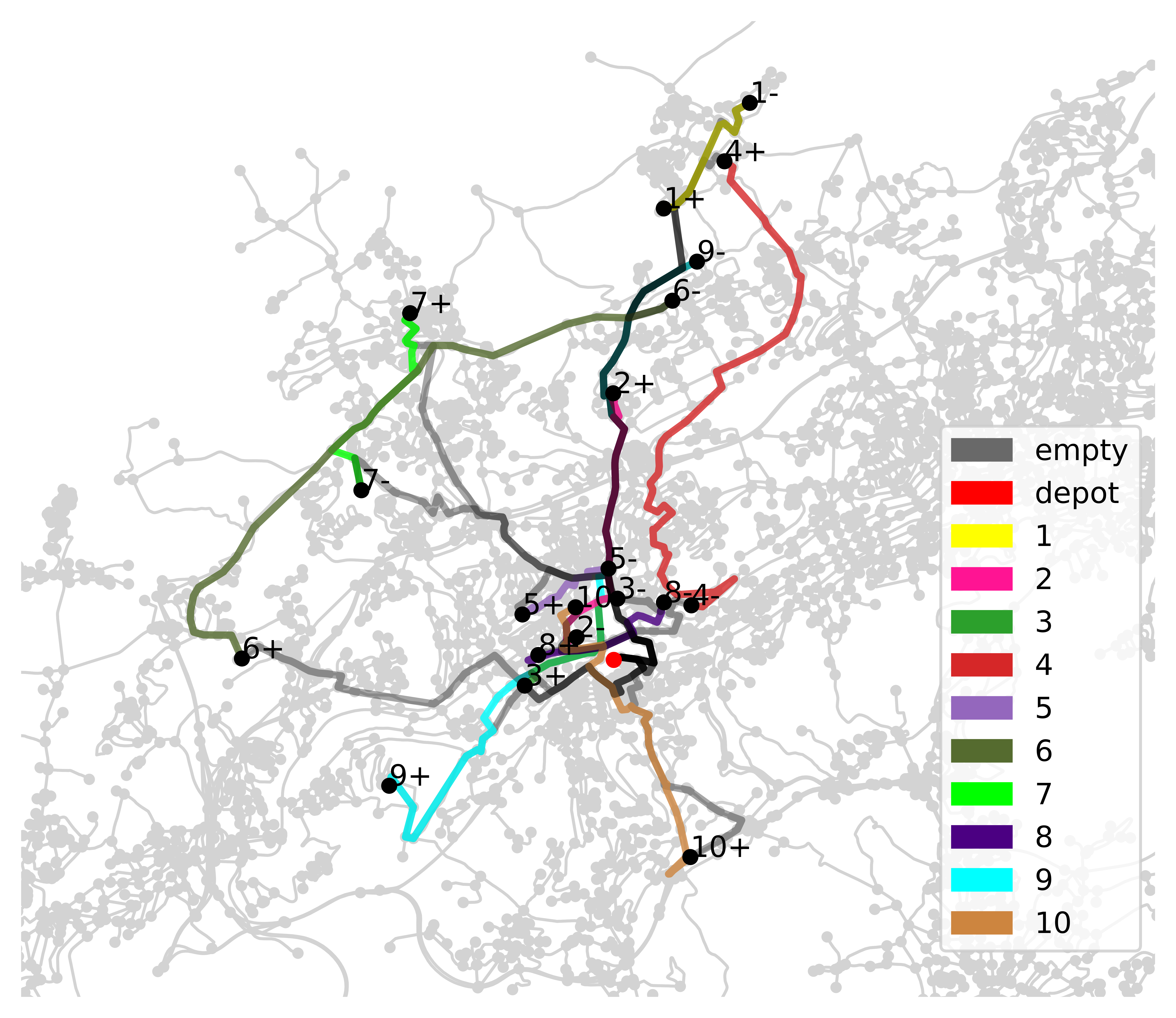
Figure 2: Vehicle routes of instance $Q3n10.3$ solved using the objective function $f_{ce}$.

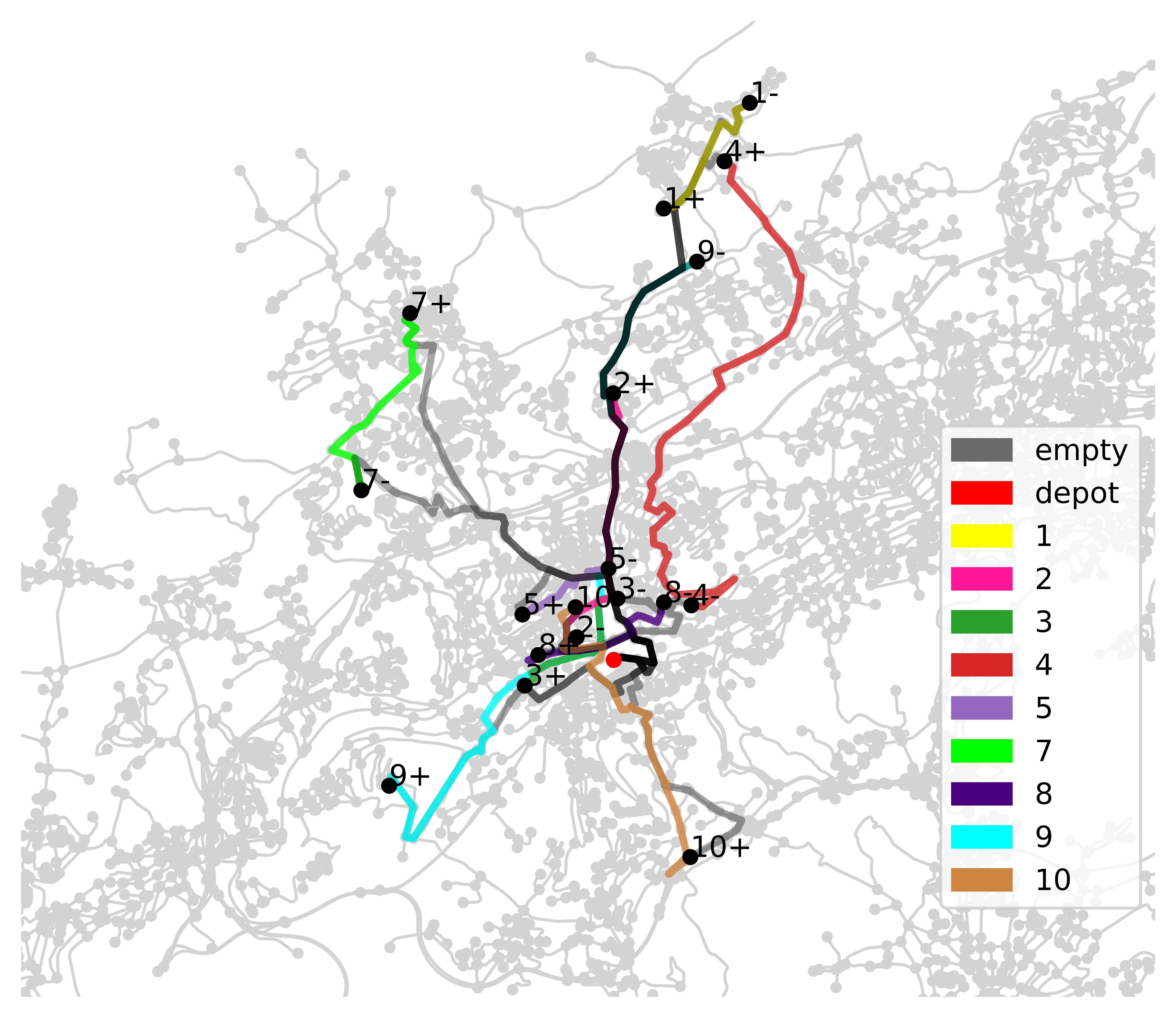
Figure 3: Vehicle routes of instance $Q3n10.3$ solved using the objective function $f_{rce}$.

[ botcap, caption = Vehicle routes (without depot) of instance $Q3n10.3$ solved using the objective functions $f_{ce}$ and $f_{rce}$., label =tab:figce, nosuper, doinside=]@ll@p0.01cmllllp0.1cmllll $f_{ce}$ $f_{rce}$
Tour 1  Location $9^{+}$ $9^{-}$ $9^{+}$ $9^{-}$
Time[m] 20.0 54.0 20.0 54.0
Tour 2 Location $3^{+}$ $3^{-}$ $2^{+}$ $2^{-}$ $3^{+}$ $3^{-}$ $2^{+}$ $2^{-}$
Time[m] 15.0 22.3 32.3 45.1 15.0 22.3 32.3 45.1
Tour 3 Location $5^{+}$ $5^{-}$ $4^{+}$ $4^{-}$ $4^{+}$ $4^{-}$
Time[m] 20.0 25.3 45.8 74. 6 35.0 63.8
Tour 4 Location $8^{+}$ $8^{-}$ $7^{+}$ $7^{-}$ $8^{+}$ $8^{-}$ $7^{+}$ $7^{-}$
Time[m] 20. 0 28.3 48.7 59.9 20. 0 28.3 48.7 59.9
Tour 5 Location $10^{+}$ $10^{-}$ $10^{+}$ $10^{-}$
Time[m] 30.0 47.0 30.0 47.0
Tour 6 Location $6^{+}$ $6^{-}$ $1^{+}$ $1^{-}$ $5^{+}$ $5^{-}$ $1^{+}$ $1^{-}$
Time[m] 20.8 49.1 57.7 65. 0 20.0 25.32 45.0 52.32

The last four columns of Table LABEL:tab:cecemaxrce, $f_{rce}$ vs. $f_{ce}$, illustrate the decrease in the overall routing costs and excess ride time that is obtained when rejecting some of the requests. This is illustrated at the instance $Q3n10.3$ in Figure 2, showing an optimal tour w.r.t. $f_{ce}$, and Figure 3 where an optimal tour w.r.t. $f_{rce}$ is shown. In Figure 2 the driver has to make a large detour to transport request $6$. When we allow to reject unprofitable requests using $f_{rce}$, variables $p_{i}\in\{0,1\}$, $i\in R$ and constraints (3) instead of $f_{ce}$ and constraints (9c) in Model II, it becomes obvious from Figure 3 that the service provider benefits from a large decrease in routing costs. Table LABEL:tab:figce contains the corresponding vehicle routes including pick-up and drop-off times in minutes after the start of service. In the vehicle tours computed using $f_{rce}$, users $1$ and $4$ are transported without any time loss.

For the Q3- and Q6-instances, on average 7% less and 3% less of the requests are answered in comparison to the results obtained with the objective function $f_{ce}$. In turn, we observe an average decrease of the total routing costs and the total excess ride time for all instance sizes. While the decrease in routing costs ranges from 2% to 11%, there are huge savings in excess ride time: There is an average decrease of 54% and 42% (Q3- and Q6-instances, respectively.) Furthermore, computational time decreases by 11% (Q3-intances) and 2% (Q6-instances).

While most real world instances of DARPs are much larger, the proposed approach could still prove useful as a subroutine also for realistically-sized instances. Particularly, the extension to the online version of DARP in which requests arrive over time could be a promising application for our models. Indeed, often only very few new requests arrive simultaneously and re-routing of already scheduled users is only acceptable if it decreases their arrival time. Consequently, the number of simultaneous users in such a rolling-horizon version of a dial-a-ride problem is relatively small and could potentially be solved exactly using one of our models. Note that this does in general not lead to a global optimal solution of the offline problem.

6 Conclusions

In this paper we suggest a new perspective on modeling ride-hailing problems. By using an event-based graph representation rather than a geographical model, we show that capacity, pairing and precedence constraints can be handled implicitly. While the resulting MILP formulations generally have more variables as compared to classical models, extensive numerical experiments show that the implicit constraint formulation leads to considerably improved computational times. Indeed, both for benchmark instances from the literature as well as for artificial instances in the city of Wuppertal, problems with up to $40$ requests can be solved within a few minutes of computational time, while problems with up to $20$ requests can be solved in less than 15 seconds. The new model is thus suitable for an incorporation into dynamic models in a rolling-horizon framework.

Moreover, we analyse the effects of including additional optimization criteria in the model. In addition to the classical cost objective function, we consider the (total or maximum) excess ride time as well as the number of rejected requests as measures for user satisfaction. By combining these criteria into a weighted sum objective function we demonstrate that user satisfaction can be largely improved at only relatively small additional expenses, i.e., overall routing costs.

In the future, we intend to use machine learning techniques to predict requests based on time series data and locate free vehicles accordingly. Furthermore, dynamic vehicle routing algorithms that take into account the traffic volume should be developed such that expected driving times can be computed with high accuracy. The goal is to communicate a reliable estinate of the expected arrival time to the customer when accepting a request.

References

- Atahran et al. (2014) A. Atahran, C. Lenté, and V. T’kindt. A multicriteria dial-a-ride problem with an ecological measure and heterogeneous vehicles. Journal of Multi-Criteria Decision Analysis, 21(5-6):279–298, 2014. doi: 10.1002/mcda.1518.
- Belhaiza (2017) S. Belhaiza. A data driven hybrid heuristic for the dial-a-ride problem with time windows. In 2017 IEEE Symposium Series on Computational Intelligence (SSCI). IEEE, nov 2017. doi: 10.1109/ssci.2017.8285366.
- Belhaiza (2019) S. Belhaiza. A hybrid adaptive large neighborhood heuristic for a real-life dial-a-ride problem. Algorithms, 12(2):39, feb 2019. doi: 10.3390/a12020039.
- Bertsimas et al. (2019) D. Bertsimas, P. Jaillet, and S. Martin. Online vehicle routing: The edge of optimization in large-scale applications. Operations Research, 67(1):143–162, 2019. doi: 10.1287/opre.2018.1763.
- Bongiovanni et al. (2019) C. Bongiovanni, M. Kaspi, and N. Geroliminis. The electric autonomous dial-a-ride problem. Transportation Research Part B: Methodological, 122:436–456, apr 2019. doi: 10.1016/j.trb.2019.03.004.
- Braekers et al. (2014) K. Braekers, A. Caris, and G. K. Janssens. Exact and meta-heuristic approach for a general heterogeneous dial-a-ride problem with multiple depots. Transportation Research Part B: Methodological, 67:166–186, 2014. doi: 10.1016/j.trb.2014.05.007.
- Chen et al. (2020) M. Chen, J. Chen, P. Yang, S. Liu, and K. Tang. A heuristic repair method for dial-a-ride problem in intracity logistic based on neighborhood shrinking. Multimedia Tools and Applications, apr 2020. doi: 10.1007/s11042-020-08894-7.
- Chevrier et al. (2012) R. Chevrier, A. Liefooghe, L. Jourdan, and C. Dhaenens. Solving a dial-a-ride problem with a hybrid evolutionary multi-objective approach: Application to demand responsive transport. Applied Soft Computing, 12(4):1247–1258, apr 2012. doi: 10.1016/j.asoc.2011.12.014.
- Cordeau (2006) J.-F. Cordeau. A branch-and-cut algorithm for the dial-a-ride problem. Operations Research, 54(3):573–586, 2006. doi: 10.1287/opre.1060.0283.
- Cordeau and Laporte (2003) J.-F. Cordeau and G. Laporte. A tabu search heuristic for the static multi-vehicle dial-a-ride problem. Transportation Research Part B: Methodological, 37(6):579–594, 2003. doi: 10.1016/s0191-2615(02)00045-0.
- Cordeau and Laporte (2007) J.-F. Cordeau and G. Laporte. The dial-a-ride problem: models and algorithms. Annals of Operations Research, 153(1):29–46, 2007. doi: 10.1007/s10479-007-0170-8.
- Cortés et al. (2010) C. E. Cortés, M. Matamala, and C. Contardo. The pickup and delivery problem with transfers: Formulation and a branch-and-cut solution method. European Journal of Operational Research, 200(3):711–724, 2010. doi: 10.1016/j.ejor.2009.01.022.
- Cubillos et al. (2009) C. Cubillos, E. Urra, and N. Rodríguez. Application of genetic algorithms for the DARPTW problem. International Journal of Computers Communications & Control, 4(2):127, 2009. doi: 10.15837/ijccc.2009.2.2420.
- Desrosiers et al. (1991) J. Desrosiers, Y. Dumas, F. Soumis, S. Taillefer, and D. Villeneuve. An algorithm for mini-clustering in handicapped transport. Les Cahiers du GERAD, G-91-02, HEC Montréal, 1991.
- Detti et al. (2017) P. Detti, F. Papalini, and G. Z. M. de Lara. A multi-depot dial-a-ride problem with heterogeneous vehicles and compatibility constraints in healthcare. Omega, 70:1–14, 2017. doi: 10.1016/j.omega.2016.08.008.
- Dumas et al. (1989) Y. Dumas, J. Desrosiers, and F. Soumis. Large scale multi-vehicle dial-a-ride problems. Les Cahiers du GERAD, G-89-30, HEC Montréal, 1989.
- Ehrgott (2005) M. Ehrgott. Multicriteria Optimization. Springer, 2005. ISBN 978-3-540-21398-7. doi: 10.1007/3-540-27659-9. URL https://doi.org/10.1007/3-540-27659-9.
- Garaix et al. (2010) T. Garaix, C. Artigues, D. Feillet, and D. Josselin. Vehicle routing problems with alternative paths: An application to on-demand transportation. European Journal of Operational Research, 204(1):62–75, jul 2010. doi: 10.1016/j.ejor.2009.10.002.
- Gschwind and Drexl (2019) T. Gschwind and M. Drexl. Adaptive large neighborhood search with a constant-time feasibility test for the dial-a-ride problem. Transportation Science, 53(2):480–491, 2019. doi: 10.1287/trsc.2018.0837.
- Gschwind and Irnich (2015) T. Gschwind and S. Irnich. Effective handling of dynamic time windows and its application to solving the dial-a-ride problem. Transportation Science, 49(2):335–354, 2015. doi: 10.1287/trsc.2014.0531.
- Guerreiro et al. (2020) P. M. M. Guerreiro, P. J. S. Cardoso, and H. C. L. Fernandes. A comparison of multiple objective algorithms in the context of a dial a ride problem. In Lecture Notes in Computer Science, pages 382–396. Springer International Publishing, 2020. doi: 10.1007/978-3-030-50436-6_28.
- Guerriero et al. (2013) F. Guerriero, M. E. Bruni, and F. Greco. A hybrid greedy randomized adaptive search heuristic to solve the dial-a-ride problem. Asia-Pacific Journal of Operational Research, 30(01):1250046, 2013. doi: 10.1142/s0217595912500467.
- Ho et al. (2018) S. C. Ho, W. Szeto, Y.-H. Kuo, J. M. Leung, M. Petering, and T. W. Tou. A survey of dial-a-ride problems: Literature review and recent developments. Transportation Research Part B: Methodological, 111:395–421, 2018. doi: 10.1016/j.trb.2018.02.001.
- Hosni et al. (2014) H. Hosni, J. Naoum-Sawaya, and H. Artail. The shared-taxi problem: Formulation and solution methods. Transportation Research Part B: Methodological, 70:303–318, 2014. doi: 10.1016/j.trb.2014.09.011.
- Hu and Chang (2014) T.-Y. Hu and C.-P. Chang. A revised branch-and-price algorithm for dial-a-ride problems with the consideration of time-dependent travel cost. Journal of Advanced Transportation, 49(6):700–723, 2014. doi: 10.1002/atr.1296.
- Hu et al. (2019) T.-Y. Hu, G.-C. Zheng, and T.-Y. Liao. Multi-objective model for dial-a-ride problems with vehicle speed considerations. Transportation Research Record: Journal of the Transportation Research Board, 2673(11):161–171, jun 2019. doi: 10.1177/0361198119848417.
- Ioachim et al. (1995) I. Ioachim, J. Desrosiers, Y. Dumas, M. M. Solomon, and D. Villeneuve. A request clustering algorithm for door-to-door handicapped transportation. Transportation Science, 29(1):63–78, 1995. doi: 10.1287/trsc.29.1.63.
- Jaw et al. (1986) J.-J. Jaw, A. R. Odoni, H. N. Psaraftis, and N. H. Wilson. A heuristic algorithm for the multi-vehicle advance request dial-a-ride problem with time windows. Transportation Research Part B: Methodological, 20(3):243–257, 1986. doi: 10.1016/0191-2615(86)90020-2.
- Jorgensen et al. (2007) R. M. Jorgensen, J. Larsen, and K. B. Bergvinsdottir. Solving the dial-a-ride problem using genetic algorithms. Journal of the Operational Research Society, 58(10):1321–1331, 2007. doi: 10.1057/palgrave.jors.2602287.
- Kirchler and Calvo (2013) D. Kirchler and R. W. Calvo. A granular tabu search algorithm for the dial-a-ride problem. Transportation Research Part B: Methodological, 56:120–135, 2013. doi: 10.1016/j.trb.2013.07.014.
- Liu et al. (2015) M. Liu, Z. Luo, and A. Lim. A branch-and-cut algorithm for a realistic dial-a-ride problem. Transportation Research Part B: Methodological, 81:267–288, 2015. doi: 10.1016/j.trb.2015.05.009.
- Luo et al. (2019) Z. Luo, M. Liu, and A. Lim. A two-phase branch-and-price-and-cut for a dial-a-ride problem in patient transportation. Transportation Science, 53(1):113–130, feb 2019. doi: 10.1287/trsc.2017.0772.
- Masmoudi et al. (2017) M. A. Masmoudi, K. Braekers, M. Masmoudi, and A. Dammak. A hybrid genetic algorithm for the heterogeneous dial-a-ride problem. Computers & Operations Res., 81:1–13, 2017. doi: 10.1016/j.cor.2016.12.008.
- Mauri et al. (2009) G. Mauri, L. Antonio, and N. Lorena. Customers' satisfaction in a dial-a-ride problem. IEEE Intelligent Transportation Systems Magazine, 1(3):6–14, 2009. doi: 10.1109/mits.2009.934641.
- Melachrinoudis et al. (2007) E. Melachrinoudis, A. B. Ilhan, and H. Min. A dial-a-ride problem for client transportation in a health-care organization. Computers & Operations Research, 34(3):742–759, mar 2007. doi: 10.1016/j.cor.2005.03.024.
- Molenbruch et al. (2017) Y. Molenbruch, K. Braekers, and A. Caris. Typology and literature review for dial-a-ride problems. Annals of Operations Research, 259(1-2):295–325, 2017. doi: 10.1007/s10479-017-2525-0.
- Paquette et al. (2013) J. Paquette, J.-F. Cordeau, G. Laporte, and M. M. Pascoal. Combining multicriteria analysis and tabu search for dial-a-ride problems. Transportation Research Part B: Methodological, 52:1–16, 2013. doi: 10.1016/j.trb.2013.02.007.
- Parragh (2011) S. N. Parragh. Introducing heterogeneous users and vehicles into models and algorithms for the dial-a-ride problem. Transportation Research Part C: Emerging Technologies, 19(5):912–930, 2011. doi: 10.1016/j.trc.2010.06.002.
- Parragh et al. (2009) S. N. Parragh, K. F. Doerner, R. F. Hartl, and X. Gandibleux. A heuristic two-phase solution approach for the multi-objective dial-a-ride problem. Networks, 54(4):227–242, dec 2009. doi: 10.1002/net.20335.
- Qu and Bard (2015) Y. Qu and J. F. Bard. A branch-and-price-and-cut algorithm for heterogeneous pickup and delivery problems with configurable vehicle capacity. Transportation Science, 49(2):254–270, 2015. doi: 10.1287/trsc.2014.0524.
- Ropke and Pisinger (2006) S. Ropke and D. Pisinger. An adaptive large neighborhood search heuristic for the pickup and delivery problem with time windows. Transportation Science, 40(4):455–472, 2006. doi: 10.1287/trsc.1050.0135.
- Ropke et al. (2007) S. Ropke, J.-F. Cordeau, and G. Laporte. Models and branch-and-cut algorithms for pickup and delivery problems with time windows. Networks, 49(4):258–272, 2007. doi: 10.1002/net.20177.
- Schilde et al. (2014) M. Schilde, K. Doerner, and R. Hartl. Integrating stochastic time-dependent travel speed in solution methods for the dynamic dial-a-ride problem. European Journal of Operational Research, 238(1):18–30, oct 2014. doi: 10.1016/j.ejor.2014.03.005.
- Souza et al. (2020) A. L. S. Souza, J. B. C. Chagas, P. H. V. Penna, and M. J. F. Souza. A hybrid heuristic algorithm for the dial-a-ride problem. In Variable Neighborhood Search, pages 53–66. Springer International Publishing, 2020. doi: 10.1007/978-3-030-44932-2_4.
- Viana et al. (2019) R. J. S. Viana, A. G. Santos, F. V. C. Martins, and E. F. Wanner. Optimization of a demand responsive transport service using multi-objective evolutionary algorithms. In Proceedings of the Genetic and Evolutionary Computation Conference Companion. ACM, jul 2019. doi: 10.1145/3319619.3328528.
- Zidi et al. (2012) I. Zidi, K. Mesghouni, K. Zidi, and K. Ghedira. A multi-objective simulated annealing for the multi-criteria dial a ride problem. Engineering Applications of Artificial Intelligence, 25(6):1121–1131, sep 2012. doi: 10.1016/j.engappai.2012.03.012.