A Variational Integrator for the Discrete Element Method

Abstract

A novel implicit integration scheme for the Discrete Element Method (DEM) based on the variational integrator approach is presented. The numerical solver provides a fully dynamical description that, notably, reduces to an energy minimisation scheme in the quasi-static limit. A detailed derivation of the numerical method is presented for the Hookean contact model and tested against an established open source DEM package that uses the velocity-Verlet integration scheme. These tests compare results for a single collision, long-term stability and statistical quantities of ensembles of particles. Numerically, the proposed integration method demonstrates equivalent accuracy to the velocity-Verlet method.

1 Introduction

Various descriptions of granular materials are compared in Figure 1, where they are classified by the treatment of the temporal and spatial dimensions, which can be either continuous or discrete. In the underlying Newtonian picture (strong form), the discrete spatial degrees of freedom (particle position and orientation) are described by continuous functions of time which are the solutions to Newton’s second law. The Discrete Element Method (DEM) [1] – a widely-adopted particle-level approach for simulating granular materials – calculates the resultant force acting on each particle during distinct time steps resulting from the discretisation of the time domain and solves the governing equation of motion. A continuum description (granular continuum) of spatially discrete systems is achieved via a micro-to-macro transition. For example Babic [2] proposed a coarse-graining method and derived a balance equation that relates continuous functions of position to each other. In practice, the micro-to-macro transitions for granular systems are often performed on discrete-time/discrete-space DEM data [3], but in principle this can be achieved for the Newtonian description too.

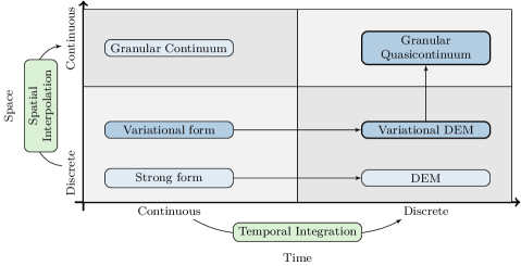
Fig. 1: A classification of descriptions of granular material based on the treatment (continuous or discrete) of the temporal and spatial dimensions. The focus of this work is a variational integrator for the Discrete Element Method which will provide the appropriate mathematical setting for a granular Quasicontinuum Method.

Unlike computational models of fluid dynamics or continuum mechanics, numerical simulation of granular materials have not been able take advantage of developments in spatial continuum modelling. Granular materials display a variety of behaviours which is often compared to the solid, fluid and gaseous phases of matter. The solid-like phase is characterised by static packing and jamming, the energetic gaseous state by pairwise collisions between particles, and the intermediate fluid-like state by dense flows [4]. Given the complexity and diversity of physical phenomena present in granular materials, finding a universal continuum description for granular material remains an open research question. A local continuum description for dense granular flow has been proposed [5, 6, 7] and have shown to be applicable in a range of situations. However, this rheology has limitations and fails to reproduce important non-local phenomena such as shear banding and arching [8, 9]. The former occurs a granular assembly is subjected to shear loading. While there is significant particle rotation and relative motion inside the shear band the remaining part of the assembly typically moves like a rigid body [10].

In the absence of a complete continuum theory, many studies of granular materials rely on discrete, particle level numerical simulations. However, in the static or slow moving phase of granular materials, a large number of particles may remain nearly stationary or behave in a manner that could be described by a continuum model. For instance, Figure 2 shows a draining silo with particles coloured by their initial vertical position. Even at an advanced state of drainage, particles in certain regions still approximately maintain their positions relative to their initial neighbours.

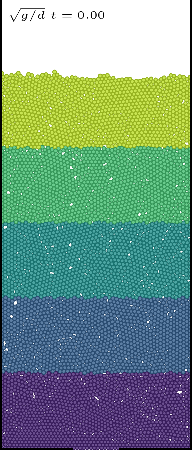
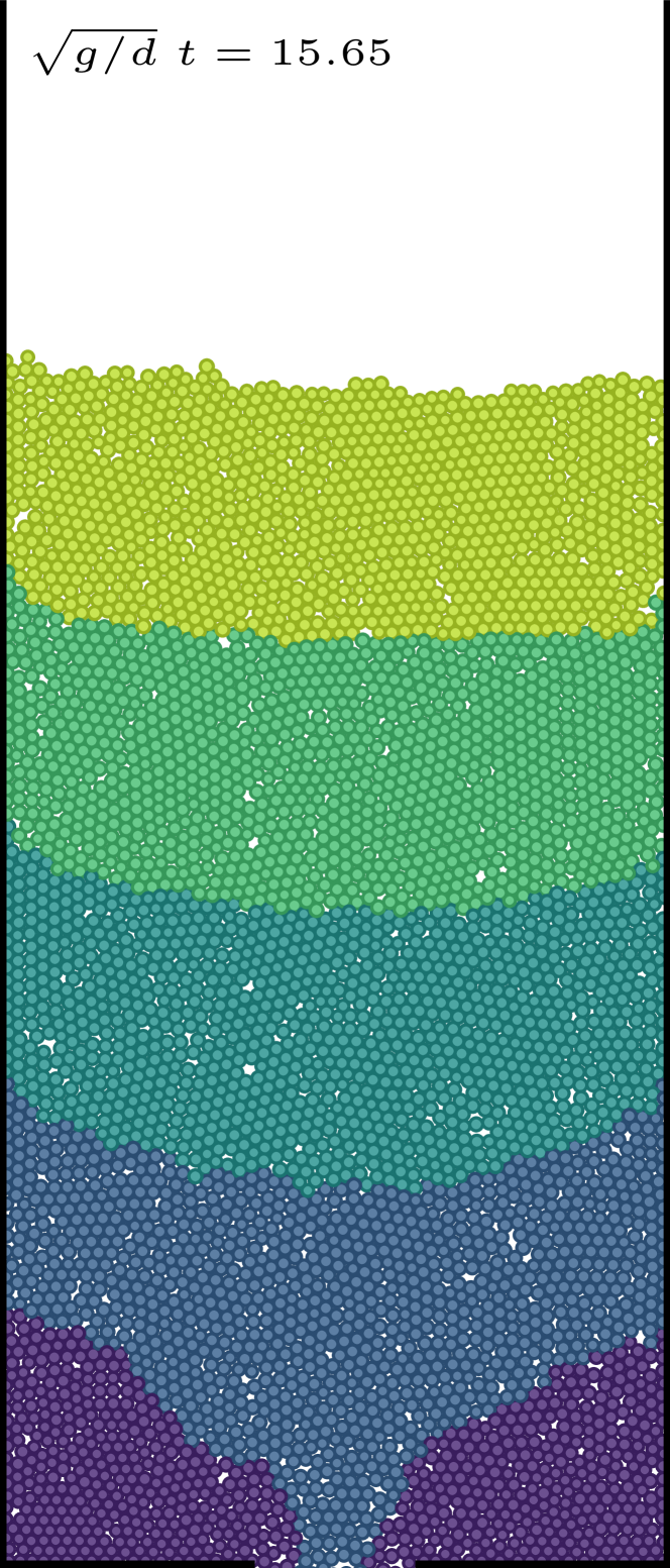
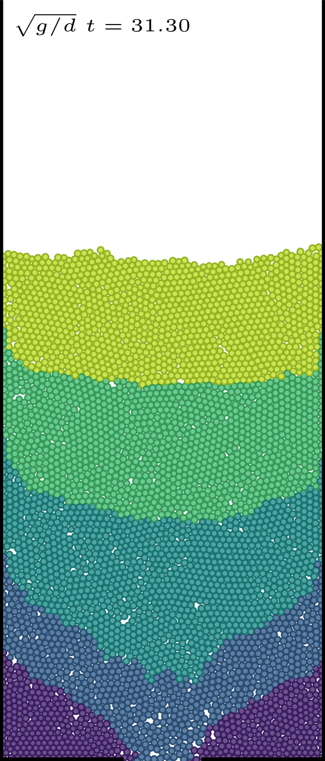
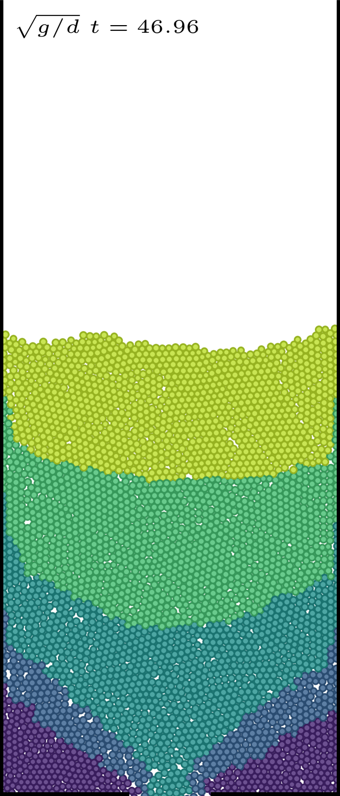
Fig. 2: A DEM simulation of a draining silo. Many particles experience only small relative displacements for the largest part of the simulation, which is common in many DEM applications.

The Quasicontinuum (QC) method is a multiscale discrete-continuum method which allows for a fully-resolved particle simulation where required, and a more efficient continuum description of material behaviour elsewhere. Simulations are carried out in a continuous spatial domain and the method thus fits to the top right quadrant of the diagram in Figure 1. The method was initially developed for crystalline atomistic simulations [11, 12, 13, 14], where the arrangement of atoms is calculated so as to minimise the global potential energy of the system using a suitable numerical technique, such as iterative energy minimisation methods. Atoms exist throughout the domain, but the computational cost is reduced by two key features. First, a series of representative atoms, or rep-atoms, are identified. The density of rep-atoms is highest in regions of specific interest and gradually diffuses toward regions of less interest. Second, the energy density is estimated by so-called summation rules in regions bordered by rep-atoms. The displacement of non rep-atoms are updated by interpolating their positions between rep-atoms. In situations where the majority of atoms fall in regions of low interest, the degrees of freedom of the simulation is greatly reduced which leads to improved simulation run time.

The objective here is to provide a temporal discretisation framework for the application of the QC method to granular systems. However, several challenges exist before a granular QC method can be realised. For the most part, with exceptions, such as [15, 16], only quasi-static configurations are simulated in the QC framework and dynamics are not accounted for. The original QC method was developed for quasi-static crystalline atomistic simulations that minimises the inter-atomic potential energy of the system. In the context of granular materials, a quasi-static simulation would restrict the method’s application to the solid-like state. To recover the dynamics, and to stay consistent with the QC approach, a novel integration method for the Discrete Element Method has been developed. The method follows Hamilton’s principle in seeking the stationary point of the action. The other hallmark of the QC method – an efficient summation rule – will be addressed in future work.

In a time continuous setting, Hamilton’s principle provides a variational scheme where the differential equations governing a dynamical system can be derived by finding the trajectory that is the stationary point of the action. The Lagrange-d’Alembert principle is a generalisation of Hamilton’s principle to non-holonomic systems, and is therefore applicable here due to the dissipative nature of granular materials. The classification in Figure 1, identifies the Hamiltonian approach (variational) to be in the same category as the Newtonian one (strong form). Variational integrators [17, 18, 19, 20, 21] are a class of algorithms where the time continuous variational principles are discretised to obtain time-stepping schemes for dynamical systems. As a result, many of the important properties of Lagrangian mechanics carry over to these algorithms. For instance, variational integrators conserve the generalised momentum of a system as a consequence of a discrete version of Noether’s theorem. Of particular interest is an implicit integration scheme, outlined in [19], that follows directly from Hamilton’s principle in a discrete setting. When the quasi-static approximation is taken, i.e. by neglecting inertia, the method simplifies to minimising the potential energy of the system – precisely what is done in the atomistic simulations that inspired the QC method. A variational integrator for DEM is the time discrete analogue to the variational format, i.e. the time discrete description in the bottom right quadrant of Figure 1, and provides a way to proceed towards the top right quadrant.

While proposing variational integrators per se is not new, the bespoke application to the Discrete Element Method is novel. This is a crucial step towards a granular Quasicontinuum method. To achieve this objective, a benchmark against current DEM solvers is needed before addressing the other challenges mentioned above. The remainder of the paper is structured as follows. Section 2 provides a detailed derivation of the variational integrator for dissipative systems and extends its application to the Hookean contact model in DEM. Section 3 discusses the implementation of the solver, shows results of numerical experiments and comparisons with established DEM codes. Section 4 is dedicated to the final discussion and conclusions.

2 Numerical Integration

The velocity-Verlet method [22] is popular in molecular dynamics and is also widely used in DEM. The same method is also known as the Strömer method and the leapfrog method, depending on the context where it is used [23]. It has been shown that the velocity-Verlet method and many of its variants can be derived using the variational integrator approach [24, 25, 23] and therefore inherits the properties of variational integrators mentioned in the introduction. However, the velocity-Verlet method is explicit and tailored toward solving Netwon’s equations in the strong form (see Figure 1) and, as discussed above, a variational approach is preferred for the Quasicontinuum method.

In practice, DEM simulations are carried out over time periods many orders of magnitude larger than the duration of a single contact which leads to a trade off between the duration and the accuracy or stability of the simulation. To ensure accurate particle trajectories, an integration time step needs to be selected that is much smaller than the duration of a contact. Choosing the optimal integration time step has been the topic of substantial research [26, 27, 28]. Implicit integration schemes have been proposed for DEM (see for instance [29, 30]). However the same limitation on the maximum time step applies, and with the added computational cost of implicit schemes these methods typically results in longer simulation times than explicit schemes. An approach to solve DEM by minimising the potential energy was proposed in [31], however this method was restricted to quasi-static configurations.

2.1 Variational Integrators

The numerical integration scheme presented here follows Kane et al. [18]. The Lagrange-d’Alembert principle (see Figure 3 (a)) is used to derive a second-order accurate integrator for the equations of motion of a general dynamical system. The continuous formulation of this principle states that for a system under the influence of a non-conservative generalised force $\boldsymbol{Q}(\boldsymbol{q},\dot{\boldsymbol{q}})$, the sum of the variation of the action ($S=\int L\ dt$) and the total work performed by the non-conservative forces is zero, that is

$$\underbrace{\delta\int_{t_{i}}^{t_{f}}L(\boldsymbol{q},\dot{\boldsymbol{q}})\ dt}_{\delta S}+\int_{t_{i}}^{t_{f}}\boldsymbol{Q}(\boldsymbol{q},\dot{\boldsymbol{q}})\cdot\delta\boldsymbol{q}\ dt=0.$$ (1)

Here $\boldsymbol{q}$ and $\dot{\boldsymbol{q}}=d\boldsymbol{q}/dt$ are the generalised coordinates and velocities, respectively, and the Lagrangian is given by $L(\boldsymbol{q},\dot{\boldsymbol{q}})=T(\dot{\boldsymbol{q}})-V(\boldsymbol{q})$, where $T(\dot{\boldsymbol{q}})$ and $V(\boldsymbol{q})$ are the kinetic and potential energy of the system, respectively.

A generalised coordinate can be any parameter that specifies the configuration of the system. For discrete particles these are the coordinates and angles that specify their position and orientation. The corresponding generalised forces are forces and torques.

In the absence of non-conservative forces ($\boldsymbol{Q}=\boldsymbol{0}$), the second term in Eq. (1) is zero and the Lagrange-d’Alembert principle is equivalent to Hamilton’s principle of least action. The Lagrange-d’Alembert principle will be required to formulate an integrator for DEM, because of the dissipative terms in the contact model. Since Hamilton’s principle is a special case, we will refer to it in the following discussion, when appropriate.

In order to find the trajectory that a system will follow in the time continuous case, the calculus of variations is used to find the stationary point of the action.

(a)

(b)

Fig. 3: Hamilton’s Principle of least action (a) is a continuous method for solving the trajectory of a dynamical system by finding the path that is the stationary point of the action. Variational integrators (b) are the discrete realisation of this principle.

For a time discrete formulation, the trajectory $\boldsymbol{q}(t)$ is decomposed into $N$ time steps of length $h$ and labelled $\{\boldsymbol{q}_{0},\cdots,\boldsymbol{q}_{N}\}$ as depicted in Figure 3 (b). A discrete Lagrangian is defined as the numerical approximation of the integral over the time step and is given by,

$$L^{\alpha}_{d}(\boldsymbol{q}_{k},\boldsymbol{q}_{k+1},h)=\int_{t}^{t+h}L(\boldsymbol{q},\dot{\boldsymbol{q}})\ dt\approx hL\left(\boldsymbol{q}_{k+\alpha},\frac{\boldsymbol{q}_{k+1}-\boldsymbol{q}_{k}}{h}\right),$$ (2)

where $\boldsymbol{q}_{k+\alpha}=[1-\alpha]\boldsymbol{q}_{k}+\alpha\boldsymbol{q}_{k+1}$. The parameter $\alpha$ is often chosen as $0$ or $1/2$ which correspond to the left hand rule or midpoint rule, respectively. The former leads to a first-order accurate integrator and the latter increases the accuracy to second-order. The discrete action is the sum over the $N$ time steps,

$$S_{d}=\sum_{k=0}^{N-1}L^{\alpha}_{d}(\boldsymbol{q}_{k},\boldsymbol{q}_{k+1},h).$$ (3)

The discrete Lagrange-d’Alembert principle [18] is given by

$$\delta\sum_{k=0}^{N-1}L^{\alpha}_{d}(\boldsymbol{q}_{k},\boldsymbol{q}_{k+1})+\sum_{k=0}^{N-1}\Big{[}\boldsymbol{Q}^{-}(\boldsymbol{q}_{k},\boldsymbol{q}_{k+1})\cdot\delta\boldsymbol{q}_{k}+\boldsymbol{Q}^{+}(\boldsymbol{q}_{k},\boldsymbol{q}_{k+1})\cdot\delta\boldsymbol{q}_{k+1}\Big{]}=0$$ (4)

where,

$$\boldsymbol{Q}^{-}_{d}(\boldsymbol{q}_{k},\boldsymbol{q}_{k+1}) =\frac{h}{2}\boldsymbol{Q}\left(\boldsymbol{q}_{k+\alpha},\frac{\boldsymbol{q}_{k+1}-\boldsymbol{q}_{k}}{h}\right),$$ (5)

$$\boldsymbol{Q}_{d}^{+}(\boldsymbol{q}_{k},\boldsymbol{q}_{k+1}) =\frac{h}{2}\boldsymbol{Q}\left(\boldsymbol{q}_{k+1-\alpha},\frac{\boldsymbol{q}_{k+1}-\boldsymbol{q}_{k}}{h}\right).$$ (6)

The equivalent of the Euler-Lagrange equations can be derived using Hamilton’s principle of stationary action. The dynamics of the system will ensure that the variation in the action, $\delta S_{d}$, remains zero for independent variations in $\delta\boldsymbol{q}_{k}$ and $\delta\boldsymbol{q}_{k+1}$, that is

$$\delta S_{d}=\sum_{k=0}^{N-1}\delta\boldsymbol{q}_{k}\cdot\frac{d}{d\boldsymbol{q}_{k}}L^{\alpha}_{d}(\boldsymbol{q}_{k},\boldsymbol{q}_{k+1},h)\ +\sum_{k=0}^{N-1}\delta\boldsymbol{q}_{k+1}\cdot\frac{d}{d\boldsymbol{q}_{k+1}}L^{\alpha}_{d}(\boldsymbol{q}_{k},\boldsymbol{q}_{k+1},h).$$ (7)

To prevent confusion with derivatives, new notation is introduced such that $D_{1}L^{\alpha}_{d}$ and $D_{2}L^{\alpha}_{d}$ are the derivative of the first and second argument of $L^{\alpha}_{d}$, respectively. Then, the index for the sum in the second term is changed to $k+1\rightarrow k$. The expression for Eq. (7) now becomes,

$$\delta S_{d}=\sum_{k=0}^{N-1}\delta\boldsymbol{q}_{k}\cdot D_{1}L^{\alpha}_{d}(\boldsymbol{q}_{k},\boldsymbol{q}_{k+1},h)\ +\sum_{k=1}^{N}\delta\boldsymbol{q}_{k}\cdot D_{2}L^{\alpha}_{d}(\boldsymbol{q}_{k-1},\boldsymbol{q}_{k},h).$$ (8)

Since $\delta\boldsymbol{q}_{0}=\delta\boldsymbol{q}_{N}=0$, the first sum can start at $k=1$ and the second can be terminated at $N-1$. Now, since both summations are carried out over the same range, the expression can be factorised, as

$$\delta S_{d}=\sum_{k=1}^{N-1}\delta\boldsymbol{q}_{k}\cdot\Big{[}D_{1}L^{\alpha}_{d}(\boldsymbol{q}_{k},\boldsymbol{q}_{k+1},h)+D_{2}L^{\alpha}_{d}(\boldsymbol{q}_{k-1},\boldsymbol{q}_{k},h)\Big{]}.$$ (9)

The condition $\delta S_{d}=0$ can be enforced by requiring that the term in the brackets be zero, that is,

$$D_{1}L^{\alpha}_{d}(\boldsymbol{q}_{k},\boldsymbol{q}_{k+1},h)+D_{2}L^{\alpha}_{d}(\boldsymbol{q}_{k-1},\boldsymbol{q}_{k},h)=\boldsymbol{0},$$ (10)

which is the discrete form of the Euler-Lagrange equation.

In the general case when dissipative forces are present (i.e. $\boldsymbol{Q}\neq\boldsymbol{0}$), the second term in Eq. (4) can be manipulated using the same steps as above to obtain,

$$\sum_{k=0}^{N-1}\Big{[}\boldsymbol{Q}_{d}^{-}(\boldsymbol{q}_{k},\boldsymbol{q}_{k+1},h)\cdot\delta\boldsymbol{q}_{k}+\boldsymbol{Q}_{d}^{+}(\boldsymbol{q}_{k},\boldsymbol{q}_{k+1})\cdot\delta\boldsymbol{q}_{k+1}\Big{]}=\sum_{k=1}^{N-1}\delta\boldsymbol{q}_{k}\cdot\Big{[}\boldsymbol{Q}_{d}^{-}(\boldsymbol{q}_{k},\boldsymbol{q}_{k+1},h)+\boldsymbol{Q}_{d}^{+}(\boldsymbol{q}_{k-1},\boldsymbol{q}_{k})\Big{]}\ .$$ (11)

The sum over $k$ and $\delta\boldsymbol{q}_{k}$ can be factored with the terms in (9), which leads to the discrete Euler-Lagrange equation,

$$D_{1}L^{\alpha}_{d}(\boldsymbol{q}_{k},\boldsymbol{q}_{k+1},h)+D_{2}L^{\alpha}_{d}(\boldsymbol{q}_{k-1},\boldsymbol{q}_{k},h)+\boldsymbol{Q}_{d}^{-}(\boldsymbol{q}_{k},\boldsymbol{q}_{k+1},h)+\boldsymbol{Q}_{d}^{+}(\boldsymbol{q}_{k-1},\boldsymbol{q}_{k},h)=\boldsymbol{0}.$$ (12)

Both Eqs. (10) and (12) are second-order equations, but a system of two first-order equations can be constructed by introducing the generalised momentum. The momentum in the time continuous case is defined by, $\boldsymbol{p}(t)=\partial L/\partial\dot{\boldsymbol{q}}$. Similarly in the time discrete setting, the momentum at step $k$ is given by

$$\boldsymbol{p}_{k}\equiv D_{2}L^{\alpha}_{d}(\boldsymbol{q}_{k-1},\boldsymbol{q}_{k},h).$$ (13)

The momentum can be used to evaluate $\boldsymbol{Q}^{+}$ at time step $k$,

$$\boldsymbol{Q}_{d}^{p}(\boldsymbol{q}_{k},\boldsymbol{p}_{k})=\frac{h}{2}\boldsymbol{Q}\left(\boldsymbol{q}_{k},\frac{\boldsymbol{p}_{k}}{m}\right)=\boldsymbol{Q}^{+}(\boldsymbol{q}_{k-1},\boldsymbol{q}_{k},h).$$ (14)

The first update equation is obtained by substituting the definition for the momentum (13) at step $k$, into the discrete Euler-Lagrange equation (12), and the second is the expression for the momentum at step $k+1$. The pair of first-order update equations is given by,

$$\boldsymbol{R}(\boldsymbol{q}_{k},\boldsymbol{q}_{k+1},\boldsymbol{p}_{k},h) \equiv\boldsymbol{p}_{k}+D_{1}L^{\alpha}_{d}(\boldsymbol{q}_{k},\boldsymbol{q}_{k+1},h)+\boldsymbol{Q}_{d}^{-}(\boldsymbol{q}_{k},\boldsymbol{q}_{k+1},h)+\boldsymbol{Q}_{d}^{p}(\boldsymbol{q}_{k},\boldsymbol{p}_{k})=\boldsymbol{0},$$ (15)

$$\boldsymbol{p}_{k+1} =D_{2}L^{\alpha}_{d}(\boldsymbol{q}_{k},\boldsymbol{q}_{k+1},h).$$ (16)

The update scheme, $(\boldsymbol{q}_{k},\boldsymbol{p}_{k})\mapsto(\boldsymbol{q}_{k+1},\boldsymbol{p}_{k+1})$, requires that the new position, $\boldsymbol{q}_{k+1}$ be calculated using an implicit scheme in Eq. (15) and then explicitly calculating the new momentum $\boldsymbol{p}_{k+1}$ using (16).

The implicit scheme for updating $\boldsymbol{q}$ is obtained by expanding (15) around $\boldsymbol{q}_{k+1}$,

$$\boldsymbol{R}(\boldsymbol{q}_{k},\boldsymbol{q}_{k+1}^{n},\boldsymbol{p}_{k},h)+\mathbf{K}(\boldsymbol{q}_{k},\boldsymbol{q}_{k+1}^{n},\boldsymbol{p}_{k},h)\Delta\boldsymbol{q}_{k+1}^{n}=\boldsymbol{0},$$ (17)

where $\boldsymbol{q}^{n}_{k+1}$ is the previous estimate for $\boldsymbol{q}_{k+1}$ and $\Delta\boldsymbol{q}_{k+1}^{n}=\boldsymbol{q}_{k+1}^{n+1}-\boldsymbol{q}_{k+1}^{n}$ is the change required to improve the estimate. The stiffness is given by,

$$\mathbf{K}(\boldsymbol{q}_{k},\boldsymbol{q}_{k+1},h) =\frac{\partial}{d\boldsymbol{q}_{k+1}}\boldsymbol{R}(\boldsymbol{q}_{k},\boldsymbol{q}_{k+1},h)$$ (18)

$$=\frac{\partial^{2}}{\partial\boldsymbol{q}_{k}\partial\boldsymbol{q}_{k+1}}L^{\alpha}_{d}(\boldsymbol{q}_{k},\boldsymbol{q}_{k+1},h)+\frac{\partial}{\partial\boldsymbol{q}_{k+1}}\boldsymbol{Q}^{-}_{d}(\boldsymbol{q}_{k},\boldsymbol{q}_{k+1},h)$$ (19)

The initial guess for $\boldsymbol{q}_{k+1}$ can be estimated using the momentum at the $k$-th time step, $\boldsymbol{q}^{0}_{k+1}=\boldsymbol{q}_{k}+h\boldsymbol{p}_{k}/m$.

2.2 Integration for DEM

DEM is characterised by treating particles as rigid bodies with ‘soft’ contacts where overlap between particles is allowed and inter-particle forces are expressed as a function of the overlap (denoted by $\delta_{ij}$). Different contact models have been proposed (for instance see [32] for a recent review), but for simplicity and without loss of generality the Hookean contact model [33, 32] is adopted. Specifically, the normal and tangential forces between particles, expressed in the global coordinate system, are calculated using

$$\boldsymbol{F}_{n_{ij}} =k_{n}\delta_{ij}\boldsymbol{n}_{ij}-\gamma_{n}m_{\mathrm{eff}}\boldsymbol{v}_{n_{ij}},$$ (20)

$$\boldsymbol{F}_{t_{ij}} =k_{t}\delta_{ij}\boldsymbol{t}_{ij}-\gamma_{t}m_{\mathrm{eff}}\boldsymbol{v}_{t_{ij}},$$ (21)

where $k_{n}$ and $k_{t}$ are the normal and tangential spring stiffness, $\gamma_{n}$ and $\gamma_{t}$ are the normal and tangential damping coefficients and $m_{\mathrm{eff}}=m_{i}m_{j}/[m_{i}+m_{j}]$ is the effective mass of the contact. The overlap, normal and tangential components of the velocity, are given by,

$$\boldsymbol{v}_{n_{ij}} =\left[\boldsymbol{v}_{ij}\cdot\boldsymbol{n}_{ij}\right]\boldsymbol{n}_{ij},$$ (22)

$$\boldsymbol{v}_{t_{ij}} =\boldsymbol{v}_{ij}-\boldsymbol{v}_{n_{ij}}-\frac{1}{2}\left[\boldsymbol{\omega}_{i}+\boldsymbol{\omega}_{j}\right]\times\boldsymbol{r}_{ij},$$ (23)

respectively, where $\boldsymbol{r}_{ij}=\boldsymbol{r}_{i}-\boldsymbol{r}_{j}$ is the relative position of the particles, $\boldsymbol{n}_{ij}=\boldsymbol{r}_{ij}/|\boldsymbol{r}_{ij}|$ is the unit vector normal to the contact, $\boldsymbol{t}_{ij}$ is unit vector tangential to the contact, $\delta_{ij}=d-|\boldsymbol{r}_{ij}|$ is the overlap between the particles with diameter $d$, $\boldsymbol{v}_{ij}=\boldsymbol{v}_{i}-\boldsymbol{v}_{j}$ is the relative velocity and $\boldsymbol{\omega}$ is the angular velocity.

The dynamics of particle $i$ is governed by the resultant force and torque,

$$\boldsymbol{F}_{i} =\boldsymbol{F}_{i}^{\mathrm{ext}}+\sum_{j}\left[\boldsymbol{F}_{n_{ij}}+\boldsymbol{F}_{t_{ij}}\right],$$ (24)

$$\boldsymbol{\tau}_{i} =-\frac{1}{2}\sum_{j}\left[\boldsymbol{r}_{ij}\times\boldsymbol{F}_{t_{ij}}\right],$$ (25)

where $\boldsymbol{F}_{i}^{\mathrm{ext}}$ are any external forces on particle $i$ and the sum $j$ is carried out over all particles that are in contact with $i$, i.e. for which $\delta_{ij}>0$.

The DEM method can be cast into the Lagrangian formulation where the Lagrangian for a system of $N_{p}$ discrete particles is given by,

$$L(\boldsymbol{q},\dot{\boldsymbol{q}})=\frac{1}{2}\dot{\boldsymbol{q}}^{T}\mathbf{M}\dot{\boldsymbol{q}}-V(\boldsymbol{q}),$$ (26)

where $\boldsymbol{q}$ is a $6N_{p}$ real column vector that represents the degrees of freedom of all $N_{p}$ particles. The integrator needs to account for the position and orientation of each particle, so a reasonable choice is to group the vector in rows of $6$, where the first $3$ entries and last $3$ entries represent the position and angular degrees of freedom, respectively. As before, the generalised velocity is $\dot{\boldsymbol{q}}=d\boldsymbol{q}/dt$ which is therefore composed of the linear and angular velocity. The generalised momentum, $\boldsymbol{p}$, contains both the linear and angular momentum. A component of $\boldsymbol{p}$ is given by $p=\partial L/\partial\dot{q}$, where $\dot{q}$ is the corresponding component of $\dot{\boldsymbol{q}}$. The mass matrix $\mathbf{M}$ is a $6N_{p}\times 6N_{p}$ diagonal matrix with blocks $\mathbf{M}_{i}=\mathrm{diag}([m_{i}\ m_{i}\ m_{i}\ I_{i}\ I_{i}\ I_{i}])$. Here $m_{i}$ and $I_{i}$ are the particle mass and moment of inertia, respectively, of particle $i$.

The first term in Eq. (26) accounts for the total kinetic energy of the system. The potential energy due to a Hookean contact between particles $i$ and $j$ is given by

$$V_{ij}=\begin{cases}\frac{k_{n}}{2}\left[\delta_{ij}\right]^{2},&\text{if }\delta_{ij}>0\\ 0,&\text{otherwise}.\end{cases}$$ (27)

The potential function is illustrated in Figure 4. This formulation can be expanded to other contact models, for instance a Hertz-Mindlin contact model can be implemented by using $V_{ij}\propto 2/5\ [\delta_{ij}]^{5/2}$ for $\delta_{ij}>0$. The potential energy for the entire system is the sum of the potentials over all the particles in contact with each other and, assuming a gravitational acceleration $\boldsymbol{g}\mathrel{\stackon[1.5pt]{=}{\stretchto{\scalerel*[width("=")]{\wedge}{\rule{4.30554pt}{12.91663pt}}}{0.5ex}}}[0,0,-g]$, the gravitational potential energy $V=\sum_{i}\sum_{j<i}V_{ij}+\sum_{i}m_{i}gz_{i}$. The generalised non-conservative forces $\boldsymbol{Q}$ in DEM are friction and velocity dependent damping terms in Eqs. (20-21).

Fig. 4: The Hookean inter-particle potential function as a function of particle overlap.

Following the prescription in Eq. (2), the discrete Lagrangian for DEM is given by,

$$L^{\alpha}_{d}(\boldsymbol{q}_{k},\boldsymbol{q}_{k+1},h)=\frac{1}{2h}\left[\boldsymbol{q}_{k+1}-\boldsymbol{q}_{k}\right]^{T}\mathbf{M}\left[\boldsymbol{q}_{k+1}-\boldsymbol{q}_{k}\right]-hV(\boldsymbol{q}_{k+\alpha}).$$ (28)

This allows one to simplify the update scheme for the integrator. The vector term in Eq. (17) becomes,

$$\boldsymbol{R}(\boldsymbol{q}_{k},\boldsymbol{q}_{k+1}^{n},\boldsymbol{p_{k}},h)=\boldsymbol{p}_{k}-\frac{1}{h}\mathbf{M}\left[\boldsymbol{q}^{n}_{k+1}-\boldsymbol{q}_{k}\right]-h\left[[1-\alpha]\frac{\partial V}{\partial\boldsymbol{q}_{k}}+\frac{1}{2}\boldsymbol{Q}^{-}(\boldsymbol{q}_{k},\boldsymbol{q}_{k+1}^{n})+\frac{1}{2}\boldsymbol{Q}^{p}(\boldsymbol{q}_{k},\boldsymbol{p}_{k})\right],$$ (29)

and the stiffness matrix,

$$\mathbf{K}(\boldsymbol{q}_{k},\boldsymbol{q}^{n}_{k+1},h)=-\frac{1}{h}\mathbf{M}-\frac{\partial}{\partial\boldsymbol{q}_{k+1}}\boldsymbol{Q}^{-}_{d}(\boldsymbol{q}_{k},\boldsymbol{q}_{k+1},h).$$ (30)

The momentum update equation (16) simplifies to

$$\boldsymbol{p}_{k+1}=D_{2}L^{\alpha}_{d}=\frac{1}{h}\mathbf{M}[\boldsymbol{q}_{k+1}-\boldsymbol{q}_{k}]-h\alpha\frac{dV}{dq_{k}}.$$ (31)

For the first-order integrator ($\alpha=0$), this can be interpreted as the product of the discrete velocity and the mass and is therefore consistent with a discrete time increment.

3 Numerical Tests

The integration scheme outlined above is implemented in the Python programming language [34, 35]. The complete algorithm is outlined in Algorithm 1. A Verlet neighbour list [22] efficiently keeps track of potential contacts and assists in constructing the residual vector and stiffness matrix. To simplify the implementation and to focus on key features of the algorithm, the tangential overlap between particles is not calculated which restricts the following numerical tests to frictionless particles ($\mu=0$).

Walls are implemented using the Hookean contact model Eqs. (20-21) by substituting the position $\boldsymbol{r}_{j}$ with the wall’s normal vector and setting $\boldsymbol{v}_{j}=\boldsymbol{0}$.

Read initial state;

Assemble $\mathbf{M}$;

$k\leftarrow 0$;

while $k<K$ do

       Detect Contacts;

      

      $\boldsymbol{q}^{0}_{k+1}\leftarrow\boldsymbol{q}_{k}+h\mathbf{M}^{-1}\boldsymbol{p}_{k}$ ;

        /* The initial guess for the position */

       $n\leftarrow 0$;

       while $E_{n}/E_{n-1}<tol$ do

             $\boldsymbol{F}\leftarrow$ Vector term in (29);

             $\mathbf{K}\leftarrow$ Matrix term in (30);

             $\Delta\boldsymbol{q}^{\Delta n}_{k+1}\leftarrow CG(\mathbf{K},-\boldsymbol{F})$ ;

              /* Solve with the conjugate gradient method */

             $\boldsymbol{q}^{n+1}_{k+1}\leftarrow\boldsymbol{q}^{n}_{k+1}+\Delta\boldsymbol{q}^{\Delta n}_{k+1}$ ;

              /* Update the guess for the next iteration */

             $E_{n-1}\leftarrow E_{n}$;

             $E_{n}\leftarrow|\ \Delta\boldsymbol{q}^{\Delta n}_{k+1}|$;

             $n\leftarrow n+1$;

            

       end while

      $\boldsymbol{q}_{k+1}\leftarrow\boldsymbol{q}^{n}_{k+1}$ ;

        /* Set the coordinates for the next iteration */

       $\boldsymbol{p}_{k+1}\leftarrow\frac{1}{h}\mathbf{M}\left[\boldsymbol{q}_{k+1}-\boldsymbol{q}_{k}\right]$ ;

        /* Update the momentum using Eq. (31) */

       $k\leftarrow k+1$;

      

end while

Algorithm 1 The first-order ($\alpha=0$) variational integrator algorithm for DEM.

A number of numerical experiments are performed to test the integrator and its implementation. Figure 5 shows the various configurations used in the tests: a collision between two particles, a single particle bouncing between two parallel walls, a collision between a bonded pair and a third particle, and an ensemble of particles settling in a box under gravity. Each case is discussed in the following sections. In each test case all particles have the same diameter and mass and the same parameters for the Hookean contact model with no friction ($\mu=0$) and normal and tangential damping is fixed to $\gamma_{t}=\gamma_{n}/2$. A damping parameter is introduced $\gamma=\gamma_{n}/m_{\mathrm{eff}}$, and different values of the parameter $\gamma$ are used to test various aspects of the integrator. In all simulations the value of the contact stiffness is fixed relative to other model parameters such that $kd/mg=$195\,000\text{\,}$$, where $g$ is gravitational acceleration and $m$ and $d$ are the particle mass and diameter, respectively.

The algorithm outlined above provides an integrator for DEM in a variational setting. In order to demonstrate that it indeed recovers the same solution as a conventional DEM simulation, comparisons are made with the results from the open source software package LAMMPS [36], where possible. LAMMPS implements a Hookean contact model [33, 37, 38]. The default velocity-Verlet [22] integrator in LAMMPS is used.

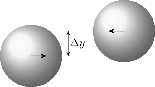
(a) Impact

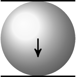
(b) Restitution between walls

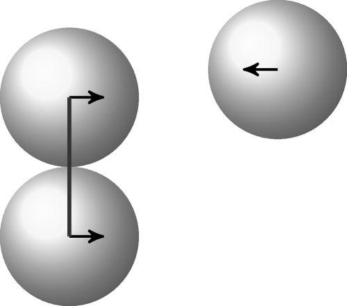
(c) Impact with a bonded pair

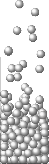
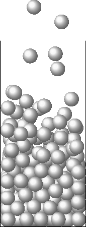
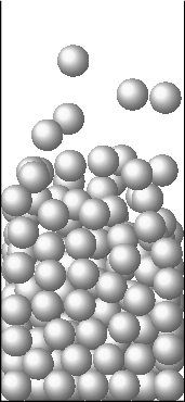
(d) Filling a box

Fig. 5: Particle configurations used for numerical experiments in this section: (a) collision between two particles, (b) a particle bouncing between walls, (c) collision with simplified bonded particles and (d) particles filling a box. Solid lines between particle centres indicate that a simplified ’bond’ was present between particles.

3.1 Two particle impact

The first test shows the numerical integration of the Hookean contact model over one collision between two particles. Simulations for different values of the integration time step $h$, damping $\gamma$ and offset $\Delta y$ (see Fig 5(a)) are performed. The two particles have initial positions $\boldsymbol{r}\mathrel{\stackon[1.5pt]{=}{\stretchto{\scalerel*[width("=")]{\wedge}{\rule{4.30554pt}{12.91663pt}}}{0.5ex}}}[d,\pm\Delta y/2,0]$ and velocities $\boldsymbol{v}\mathrel{\stackon[1.5pt]{=}{\stretchto{\scalerel*[width("=")]{\wedge}{\rule{4.30554pt}{12.91663pt}}}{0.5ex}}}[\mp v,0,0]$.

An analytical solution is available for the special case when $\Delta y=0$, as all contributions from tangential forces remain zero. The time at which the collision starts can be calculated and is given by $t_{A}=d/2v$. After this time, the force between the particles is given by

$$F=k_{n}[d-x]+\frac{1}{2}\gamma mv,$$ (32)

where $[x,0,0]$ and $[-v,0,0]$ is the position and velocity, respectively, of the particle on the right. This is the same force as a damped simple harmonic oscillator for which the position and velocity are given by:

$$x(t) =\frac{d}{2}-vt_{\gamma}\exp\left(-\frac{\gamma\ t}{m}\right)\sin\left(\frac{t}{t_{\gamma}}\right),$$ (33)

$$v(t) =v\exp\left(-\frac{\gamma t}{m}\right)\left[\frac{\gamma^{2}}{m}\sin\left(\frac{t}{t_{\gamma}}\right)-\cos\left(\frac{t}{t_{\gamma}}\right)\right],$$ (34)

where $t_{\gamma}=\left[2k/m-[\gamma/m]^{2}\right]^{-1/2}$. The duration of the collision can also be calculated by solving for $t$ in $x(t)=d/2$, which gives $t_{C}=\pi\sqrt{m/(2k)}$.

Figures 6 to 8 show the translational and rotational kinetic energy of the particle on the right over the course of the collision. The translational kinetic energy was calculated as $K_{T}=1/2\ m[v_{x}^{2}+v_{y}^{2}]$, where $\boldsymbol{v}\mathrel{\stackon[1.5pt]{=}{\stretchto{\scalerel*[width("=")]{\wedge}{\rule{4.30554pt}{12.91663pt}}}{0.5ex}}}[v_{x},v_{y},0]$ is the particle velocity, and rotational kinetic energy $K_{R}=1/2\ I\omega_{z}^{2}$, where $I=2/5\ m[d/2]^{2}$ is the moment of inertia of a sphere and $\omega_{z}$ is the rotational velocity around the $z$ axis. Figures 6(a) and 6(b) shows results of the proposed integrator for a small time step $h\approx t_{c}/160$. For this time step size there is excellent agreement with LAMMPS and results between the two integrators are indistinguishable. Comparisons between the first and second-order integrators and LAMMPS at larger time steps ($h\approx{t_{c}/3.2,t_{c}/16.1}$, $\Delta y/d=0.1$ and $\gamma=30$) are made in Figure 7(a) and 7(b). The second-order integrator compares well with LAMMPS in the case when $h=t_{c}/16.1$, but the amount of energy dissipated is (not surprisingly) incorrectly calculated for large time steps $h=t_{c}/3.2$ by all integrators tested. Finally, Figure 8 compares the second-order integrator (with $h\approx t_{c}/160$ and $\Delta y=0$) to the analytic solution in equation (34) and demonstrates near exact agreement.

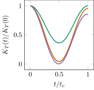
(a)

(b)

Fig. 6: Two particle impact: Kinetic energy of one particle for small integration time steps ($h\approx t_{c}/160$) and various parameters. Results between the proposed integrator and LAMMPS are indistinguishable.

(a)

(b)

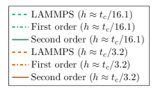
Fig. 7: Two particle impact: Kinetic energy of one particle for large integration time steps ($h\approx{t_{c}/3.2,t_{c}/16.1}$) and $\Delta y/d=0.1$ and $\gamma=30$. There is agreement between LAMMPS and the second-order integrator for $h\approx t_{c}/16.1$, but the energy dissipation over the course of the collision is not correctly calculated for the very large time step $h\approx t_{c}/3.2$.

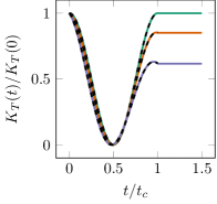
Fig. 8: Two particle impact: Kinetic energy of one particle ($h\approx t_{c}/160$, $\Delta y=0$) compared to the analytic solution in equation (34).

3.2 Particle bouncing between walls

Variational integrators are known to display excellent energy conservation, despite the fact that energy conservation is not guaranteed [18]. To test the energy conservation behaviour of the variational integrator, a simulation is performed where a particle is placed between two parallel walls set $1.01d$ apart. The particle’s initial velocity is perpendicular to them (see Figure 5(b)). In the undamped case ($\gamma_{t}=\gamma_{n}=0$), the particle will bounce between the walls without loss of energy and thereby provide a good test for the energy conserving properties of the integrator. During the brief periods of no contact the total energy in the system will be the particle’s kinetic energy and during a collision some energy will be converted to potential energy $V=1/2\ k_{n}\delta^{2}$, where $\delta$ is the overlap between the particle and wall.

The total energy of the particle is plotted in Figure 9. The total energy is the sum of the kinetic energy and potential energy of the Hookean contact. The simulation is carried out over $250$ collisions, but the graph shows the total energy for the last few collisions. For $h\approx t_{c}/32$, the second-order integrator looses a small fraction ($\sim 0.1\%$) of energy over the course of the simulation. The total energy of the LAMMPS simulation is not exactly conserved, but remains bounded. However, the energy loss of the variational integrator is dependent on the time step and when the time step is reduced to $h\approx t_{c}/160$, the energy loss in the variational integrator is similar to the fluctuations in the energy produced by the velocity-Verlet integrator used in LAMMPS.

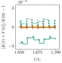
(a)

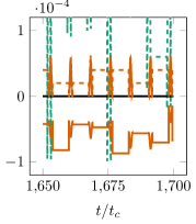
(b)

Fig. 9: The total energy of a particle bouncing between walls after $250$ collisions. A magnified section of (a) is shown in (b). Some energy is lost by the variational integrator, but for small time steps this is equivalent to the bounded fluctuation produced by the velocity-Verlet integrator used in LAMMPS.

3.3 Impact with a bonded pair

A simple bonded particle contact model is implemented by allowing attractive forces between particles. This is implemented by creating a ’bond’ between particles if in the initial configuration they are close together ($|\delta_{ij}|<d/100$). Whenever a bond exists between particles, the potential $V_{ij}=k_{n}[\delta_{ij}]^{2}/2$ was used even when particles were separated.

A simulation is performed of a collision between a pair of bonded particles and a third unbonded particle. The purpose of this is to test the simplified bonded particle model and test the integrator with contact models that have different time scales. Different time scales can be introduced by choosing different spring stiffness constants for regular Hookean interactions ($k$) and bonded contacts ($k_{B}$).

The initial setup is similar to the two particle impact simulation, except that one of the particles is replaced by a bonded pair, see Figure 10. The bonded particles are given the same initial velocity.

The bond between the two particles on the left prevents them from separating after the impact, Figure 10(a) shows the particles and their trajectories after the collision. The magnitudes of two inter-particle forces are shown in Figure 10(b). The collision between particles $1$ and $2$ produces a peak at the impact. After the collision, the bond produces an oscillation in the force between particles $1$ and $3$. The maximum integration time step size is determined by the smallest time scale ($\min\{\sqrt{2k/m},\sqrt{2k_{B}/m}\}$).

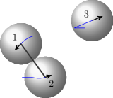
(a)

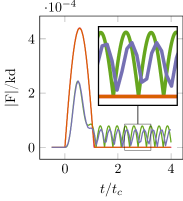
(b)

Fig. 10: Impact with a bonded pair: the configuration of particles (a) before and (b) after the collision. The trajectories of the particles are denoted by blue lines. The inter-particle forces are compared in (c), particles $1\text{\,}$ and $2\text{\,}\mathrm{e}$xperience a force due to the bond between them and a Hookean contact force is present momentarily between $1\text{\,}$ and $3\text{\,}$.

3.4 Filling a box

To investigate a less academic test case, the variational integration scheme is employed to simulate an ensemble of particles. A LAMMPS simulation was run to create an initial condition consisting of $N_{p}=218$ particles in a $L\times L\times 20L$ (with $L=6d$) box. A gravitational force was applied in the $[0,0,-1]$ direction A snapshot of the simulation captured before all the particles had settled in the bottom of the box was used as the starting configuration of further tests. The simulation was continued in LAMMPS and the variational integrator until all the particles settled at the bottom of the box.

When making comparisons between simulations with ensembles of particles, the sensitivity of these systems to initial conditions and small numerical errors must be kept in mind. Instead of focusing on individual particle positions and velocities, macroscopic quantities are compared. Here, the average kinetic energy per particle and velocity fluctuations (which is related to the granular temperature) of the ensemble are shown as the simulation progress. These quantities are calculated as

$$\bar{K} =\frac{1}{2N_{p}}\sum_{i=1}^{N_{P}}\left\{m\left[[v^{i}_{x}]^{2}+[v^{i}_{y}]^{2}+[v^{i}_{z}]^{2}\right]+I\left[\omega^{2}_{x}+\omega^{2}_{y}+\omega^{2}_{z}\right]\right\},$$ (35)

$$\delta v =\frac{1}{3N_{P}}\sum_{i=1}^{N_{P}}\left[[\bar{v}_{x}-v^{i}_{x}]^{2}+[\bar{v}_{y}-v^{i}_{y}]^{2}+[\bar{v}_{z}-v^{i}_{z}]^{2}\right],$$ (36)

where bars denote average velocity components: $\bar{v}_{x}=\sum_{i}^{N_{P}}v^{i}_{x}/N_{P}$.

The results are presented in Figure 11 as a function of the simulation time. A particle system such as this is known to be sensitive to initial conditions and numerical errors, so particle trajectories diverge after a few collisions even for the same integration method with different time steps. However, the physically meaningful values such as the the coarse-grained statistical quantities presented show excellent agreement with LAMMPS.

(a)

(b)

Fig. 11: Macroscopic quantities (a) kinetic energy and (b) kinetic stress of $N_{p}=218$ particles settling in a box under gravity.

4 Conclusion

A variational integrator for DEM has been described and implemented for the Hookean contact model. Our implicit scheme has been compared against the velocity-Verlet method implemented in LAMMPS. Excellent accuracy has been observed at the micro scale (integration over a single collision), macro scale (particles setting in box) as well as good long-term stability (particle bouncing between walls). A simplified bonded particle model has been implemented, thereby demonstrating the method’s versatility and the ability to include other contact models.

Using an implicit numerical method, there is additional computational expense when compared to explicit methods. However, as a variational integrator our approach is attractive since it is a discrete realisation of the Lagrange-d’Alembert principle, an extension of Hamilton’s principle to non-conservative systems, that computes the trajectories of particles by finding the stationary point of the action. Therefore, it represents a dynamical extension of the atomistic simulations based on the quasi-static energy minimisation principle that inspired the Quasicontinuum (QC) method. Thus, in a fully realised granular QC method, as motivated in Figure 1, the computational cost of using an implicit integration scheme will be offset by the reduced degrees of freedom of the simulation. Indeed, in our future work will focus on developing a suitable granular QC method, including appropriate summation rules.

References

- Cundall and Strack [1979] P. A. Cundall, O. D. L. Strack, A discreate numerical model for granular assemblies, Geotechnique 29 (1979) 47–65.
- Babic [1997] M. Babic, Average balance equations for granular materials, Int. J. Eng. Sci. 35 (1997) 523–548.
- Miehe and Dettmar [2004] C. Miehe, J. Dettmar, A framework for micro-macro transitions in periodic particle aggregates of granular materials, Comput. Methods Appl. Mech. Eng. 193 (2004) 225–256.
- Jaeger et al. [1996] H. M. Jaeger, S. R. Nagel, R. P. Behringer, Granular solids, liquids, and gases, Rev. Mod. Phys. 68 (1996) 1259–1273.
- GDR MiDi [2004] GDR MiDi, On dense granular flows., Eur. Phys. J. E. Soft Matter 14 (2004) 341–365.
- Da Cruz et al. [2005] F. Da Cruz, S. Emam, M. Prochnow, J.-N. Roux, F. Chevoir, Rheophysics of dense granular materials : Discrete simulation of plane shear flows, Phys. Rev. E 72 (2005) 021309.
- Jop et al. [2006] P. Jop, Y. Forterre, O. Pouliquen, A constitutive law for dense granular flows, Nature 441 (2006) 727–730.
- Jop [2015] P. Jop, Rheological properties of dense granular flows, Comptes Rendus Phys. 16 (2015) 62–72.
- Kamrin [2019] K. Kamrin, Non-locality in Granular Flow: Phenomenology and Modeling Approaches, Front. Phys. 7 (2019) 1–7.
- Gao and Zhao [2013] Z. Gao, J. Zhao, Strain localization and fabric evolution in sand, Int. J. Solids Struct. 50 (2013) 3634–3648.
- Tadmor et al. [1996] E. B. Tadmor, M. Ortiz, R. Phillips, Quasicontinuum analysis of defects in solids, Philos. Mag. A 73 (1996) 1529–1563.
- Knap and Ortiz [2001] J. Knap, M. Ortiz, An analysis of the quasicontinuum method, J. Mech. Phys. Solids 49 (2001) 1899–1923.
- Miller and Tadmor [2002] R. E. Miller, E. B. Tadmor, The Quasicontinuum Method: Overview, applications and current directions, J. Comput. Mater. Des. 9 (2002) 203–239.
- Tadmor and Miller [2005] E. B. Tadmor, R. E. Miller, The Theory and Implementation of the Quasicontinuum Method, in: S. Yip (Ed.), Handb. Mater. Model., Springer Netherlands, Dordrecht, 2005, pp. 663–682. URL: http://link.springer.com/10.1007/978-1-4020-3286-8_34. doi:10.1007/978-1-4020-3286-8_34.
- Kochmann and Venturini [2014] D. M. Kochmann, G. N. Venturini, A meshless quasicontinuum method based on local maximum-entropy interpolation, Model. Simul. Mater. Sci. Eng. 22 (2014).
- Amelang et al. [2015] J. S. Amelang, G. N. Venturini, D. M. Kochmann, Summation rules for a fully nonlocal energy-based quasicontinuum method, J. Mech. Phys. Solids 82 (2015) 378–413.
- Marsden et al. [1999] J. E. Marsden, S. Pekarsky, S. Shkoller, Discrete Euler-Poincaré and Lie-Poisson equations, Nonlinearity 12 (1999) 1647–1662.
- Kane et al. [2000] C. Kane, J. E. Marsden, M. Ortiz, M. West, Variational integrators and the Newmark algorithm for conservative and dissipative mechanical systems, Int. J. Numer. Methods Eng. 49 (2000) 1295–1325.
- Marsden and West [2001] J. E. Marsden, M. West, Discrete mechanics and variational integrators, Acta Numer. 10 (2001) 357–514.
- Lew et al. [2004a] A. Lew, J. E. Marsden, M. Ortiz, M. West, An Overview of Variational Integrators, in: A. M. L. P. Franca, T. E. Tezduyar (Ed.), Finite Elem. Methods 1970’s Beyond, International Center for Numerical Methods in Engineering (CIMNE), Barcelona, 2004a. URL: https://resolver.caltech.edu/CaltechAUTHORS:20101005-091206576.
- Lew et al. [2004b] A. Lew, J. E. Marsden, M. Ortiz, M. West, Variational time integrators, Int. J. Numer. Methods Eng. 60 (2004b) 153–212.
- Verlet [1967] L. Verlet, Computer "Experiments" on Classical Fluids. I. Thermodynamical Properties of Lennard-Jones Molecules, Phys. Rev. 159 (1967) 98–103.
- Hairer et al. [2003] E. Hairer, C. Lubich, G. Wanner, Geometric numerical integration illustrated by the Störmer–Verlet method, Acta Numer. 12 (2003) 399–450.
- Ruth [1983] R. Ruth, A canonical integration technique, IEEE Trans. Nuc. Sci. 30 (1983) 2669–2671.
- Leimkuhler and Skeel [1994] B. J. Leimkuhler, R. D. Skeel, Symplectic Numerical Integrators in Constrained Hamiltonian Systems, J. Comput. Phys. 112 (1994) 117–125.
- O’Sullivan and Bray [2004] C. O’Sullivan, J. D. Bray, Selecting a suitable time step for discrete element simulations that use the central difference time integration scheme, Eng. Comput. (Swansea, Wales) 21 (2004) 278–303.
- Washino et al. [2016] K. Washino, E. L. Chan, K. Miyazaki, T. Tsuji, T. Tanaka, Time step criteria in DEM simulation of wet particles in viscosity dominant systems, Powder Technol. 302 (2016) 100–107.
- Otsubo et al. [2017] M. Otsubo, C. O’Sullivan, T. Shire, Empirical assessment of the critical time increment in explicit particulate discrete element method simulations, Comput. Geotech. 86 (2017) 67–79.
- Ke and Bray [1995] T. C. Ke, J. Bray, Modeling of particulate media using discontinuous deformation analysis, J. Eng. Mech. 121 (1995) 1234–1243.
- Samiei et al. [2013] K. Samiei, B. Peters, M. Bolten, A. Frommer, Assessment of the potentials of implicit integration method in discrete element modelling of granular matter, Comput. Chem. Eng. 49 (2013) 183–193.
- Krijgsman and Luding [2016] D. Krijgsman, S. Luding, Simulating granular materials by energy minimization, Comput. Part. Mech. 3 (2016) 463–475.
- Rojek [2018] J. Rojek, Contact Modeling in the Discrete Element Method, in: A. Popp, P. Wriggers (Eds.), Contact Model. Solids Part., volume 585, Springer International Publishing, 2018, pp. 177–228. URL: http://link.springer.com/10.1007/978-3-319-90155-8_4. doi:10.1007/978-3-319-90155-8_4.
- Silbert et al. [2001] L. E. Silbert, D. Ertaş, G. S. Grest, T. C. Halsey, D. Levine, S. J. Plimpton, Granular flow down an inclined plane: Bagnold scaling and rheology, Phys. Rev. E 64 (2001) 051302.
- Python Software Foundation [2020] Python Software Foundation, Python Language Reference version 3.8.5, 2020. URL: www.python.org.
- Van Rossum [1994] G. Van Rossum, Python Tutorial, Technical Report, Centrum voor Wiskunde en Informatica (CWI), Amsterdam, 1994.
- Plimpton [1995] S. Plimpton, Fast Parallel Algorithms for Short-Range Molecular Dynamics, J. Comput. Phys. 117 (1995) 1–19.
- Brilliantov et al. [1996] N. V. Brilliantov, F. Spahn, J.-M. Hertzsch, T. Pöschel, Model for collisions in granular gases, Phys. Rev. E 53 (1996) 5382–5392.
- Zhang and Makse [2005] H. P. Zhang, H. A. Makse, Jamming transition in emulsions and granular materials, Phys. Rev. E 72 (2005) 011301.