[2103.01753] 1 Introduction

Accuracy of the recovered flux of extended sources obscured by bad pixels in the central EPIC FOV

XMM-SOC-CAL-TN-0227

J. Nevalainen, I. Valtchahov, R. D. Saxton and S. Molendi

Feb 2 2021

1 Introduction

A fraction of the XMM-Newton EPIC FOV is obscured by the dysfunctional (i.e. bad) pixels, dominated by the CCD gaps, which complicates the analysis of extended X-ray sources. Before SAS version 17.0.0 the only standard option for attempting the recovery of the obscured flux was to scale the measured flux by the fraction of the obscured detector area. This is accurate only in the very limiting case of an extended source with a uniform spatial flux distribution.

Since version 17.0.0 SAS has included an option for recovering the lost fraction of the flux obtained by a primary instrument (e.g. pn) by utilising the information of the spatial distribution of the flux (i.e. an image) of the same source observed with another instrument (e.g. MOS2). Assuming that the supplementary image is minimally obscured at the spatial locations where the primary instrument is obscured, the correction can be accurate.

The procedure is implemented to arfgen whereby the effective area associated with the input spectrum is reduced by the lost flux fraction in the intended full extraction region, as informed by the supplementary image. While it is the flux, rather than the effective area, that is reduced in reality, the above correction works in practice. Namely, when using the effective area, reduced by the above procedure, in the consequent spectral fitting of the data reduced by the bad pixel obscuration by the same factor, the net effect is the increase of the spectral emission model normalisation compared to that obtained with the original effective area. The increased model normalisation corresponds to the full unobscured extraction region, as desired.

Since the fraction of the obscured area may exceed 10% in the EPIC FOV (see below) the knowledge of the accuracy of the recovery procedure is important if one is interested in a high level of accuracy of the recovered flux of an extended source in the full intended extraction region. Our aim in this note is to evaluate the accuracy achieved by the recommended default procedure using a sample of clusters of galaxies. We do not examine here the accuracy of the recovery of the spectral shape since its change is expected to be small in general compared to the flux effect.

2 Data

2.1 The sample

We used a sample of 27 XMM-Newton observations of nearby (z $<$ 0.1) clusters of galaxies for our work (see Table 1). Galaxy clusters are useful because their stable, bright and diffuse X-ray emission fills completely the central regions of the EPIC FOV, providing sufficient numbers of counts within the pixels of our adopted size of 5 arcsec (see Section 3.1). Also, the surface brightness of clusters decreases quite rapidly with the distance from the cluster center (see Section 3.2.2) which is essential for the testing of the recovery of the obscured non-uniform flux. We limit the study within 6 arcmin distance from the cluster center in order to maintain the background below 10% of the cluster emission in the adopted 0.5-7.0 keV energy band.

2.2 Processing

When processing the data and extracting products for generating the effective area files (i.e. event files, spectra and images), we intended to mimic the choices of a general user for wider applicability of our results, i.e. we use default procedures and parameter values. We processed the pn and MOS event files with epchain and emchain procedures, respectively, in SAS18.0.0 with default parameters. Relevant for our analysis, the epchain default setting runbadpixfind=Y will cause the badpixfind routine to be executed. In the default mode 1 (enabled by searchbadpix=Y) hot, dead and flickering pixels in a given observation are identified. In case of emchain, the default setting (badpixfindalgo=EM) activates a more sensitive embadpixfind routine, instead of badpixfind routine used for pn.

The default settings runbadpix=Y for epchain and withbadpix=yes for emchain activate the badpix routine with getnewbadpix=Y whereby the bad pixels identified above will be propagated to the BADPIX extension of the event files. The default settings getuplnkbadpix=Y and getotherbadpix=Y propagate the uplinked and non-uplinked bad pixels to the BADPIX extension.

We then filtered the pn and MOS event files with the recommended expressions

FLAG==0 && PATTERN<=4

and

#XMMEA_EM && PATTERN<=12

We further filtered the event files by removing the data obtained during flare periods. These event files (e.g. pn.fits) will be used as arguments for the badpixlocation parameter when running arfgen in Section 3.1.

We extracted spectra with default parameters within central r = 6 arcmin region (defined in sky coordinates) centered at the X-ray peak (see Table 1). We did not exclude point sources except in the case of A2142, where an exceptionally bright source is partially obscured by a pn CCD gap. These spectra (e.g. pn.pha) will be used as arguments for the spectrumset parameter when running arfgen in Section 3.1.

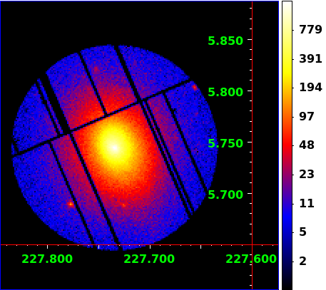
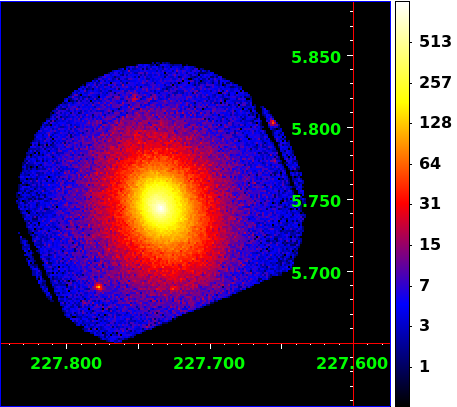
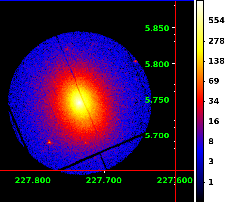
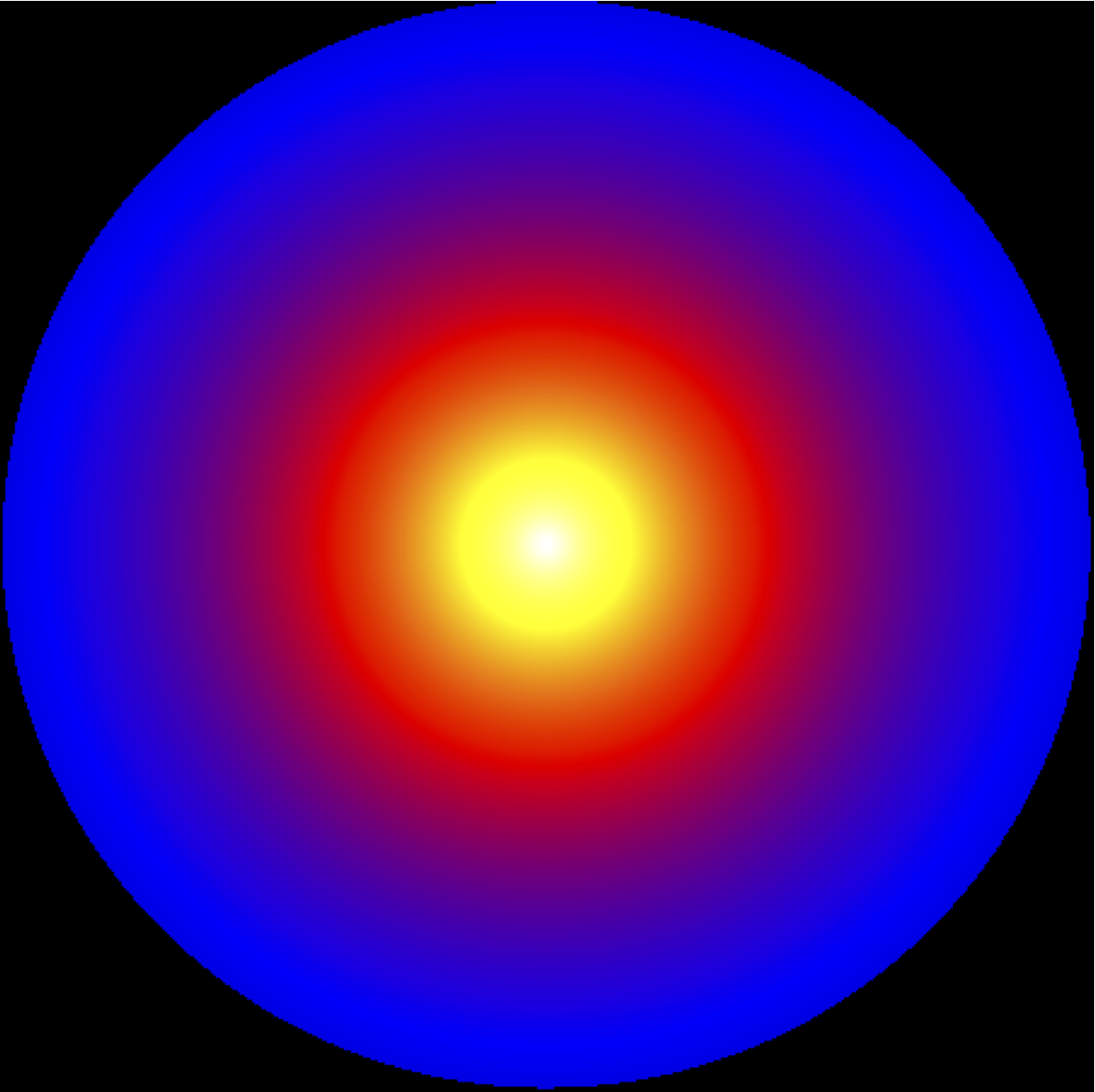
We extracted raw count MOS2 images within central r = 6 arcmin region in the sky coordinate system with a bin size of 5 arcsec in the 0.5-7.0 keV band. These images (e.g. MOS2.im, see Fig. 1) will be used as arguments for the detmaparray parameter when running arfgen in Section 3.1.

In order to obtain estimates of the geometric fraction R_area of the unobscured area to that of the full intended circle with r = 6 arcmin, we utilised the backscale - routine with withbadpixcorr=yes, badpixelresolution=1 (1 arcsec) and badpixlocation set to the event file produced above (e.g. pn.fits). The computations yielded that on average the pure geometric area reduction factor due to bad pixel/CCD gap obscuration (1 - $<$ R ${}_{area}>$ ) is 14% for pn, 5% for MOS1 and 4% for MOS2 for our sample (see Table 1).

Refer to caption — Figure 1: Raw count images of A2029 cluster (OBSID = 0551780301) using pn (left panel), MOS1 (middle panel) and MOS2 (right panel) in sky coordinates in the central r = 6 arcmin region. The color bars indicate the level of counts per pixel.

Table 1: Results

cluster	Obs. ID	RA	DEC	R_area^a			R_image^b	R_model^c
				————————
				pn	M1	M2
A85	0723802101	10.460333	-9.303008	0.866	0.932	0.963	0.8819	0.8851
A85	0723802201	10.460333	-9.303008	0.866	0.933	0.965	0.8807	0.8846
A401	0112260301	44.740833	13.582642	0.862	0.960	0.966	0.8564	0.8496
A478	0109880101	63.354875	10.465269	0.860	0.965	0.972	0.8828	0.8898
A644	0744412201	124.356792	-7.512367	0.867	0.931	0.960	0.8962	0.8837
A754	0136740101	137.333375	-9.679144	0.849	0.969	0.972	0.8607	0.8595
A1650	0093200101	194.673000	-1.761561	0.847	0.958	0.958	0.8327	0.8287
A1651	0203020101	194.843583	-4.196039	0.867	0.960	0.965	0.8758	0.8811
A1795	0097820101	207.220833	26.590278	0.887	0.962	0.965	0.9087	0.9035
A2029	0551780301	227.734167	5.744639	0.871	0.899	0.963	0.9312	0.9278
A2142	0674560201	239.583208	27.233158	0.865	0.945	0.951	0.8659	0.8742
A2244	0740900101	255.676958	34.060236	0.866	0.929	0.961	0.8906	0.8917
A2319	0302150101	290.297333	43.949839	0.863	0.960	0.960	0.8752	0.8779
A2319	0302150201	290.297333	43.949839	0.873	0.859	0.965	0.8901	0.8895
A2319	0600040101	290.297333	43.949839	0.866	0.954	0.962	0.8698	0.8643
A3112	0603050101	49.490417	-44.238417	0.866	0.947	0.960	0.9070	0.9090
A3391	0505210401	96.585067	-53.693201	0.866	0.959	0.967	0.8511	0.8622
A3558	0107260101	201.987125	-31.495583	0.868	0.966	0.966	0.8750	0.8788
A3571	0086950201	206.867667	-32.864533	0.867	0.965	0.968	0.8745	0.8713
A3827	0149670101	330.469708	-59.946483	0.865	0.962	0.969	0.8723	0.8695
Coma	0300530101	194.954625	27.960983	0.858	0.906	0.960	0.8686	0.8590
Coma	0153750101	194.954625	27.960983	0.864	0.968	0.973	0.8661	0.8665
CygA	0302800101	299.868042	40.733919	0.867	0.954	0.962	0.9073	0.9022
PKS0745	0105870101	116.880417	-19.294394	0.865	0.961	0.965	0.9055	0.9146
Ophiuchus	0505150101	258.115500	-23.368714	0.865	0.955	0.961	0.8671	0.8630
Triangulum	0093620101	249.583167	-64.356086	0.854	0.964	0.970	0.8525	0.8469
ZwCl1215	0300211401	184.421333	3.655767	0.866	0.944	0.962	0.8637	0.8696

^a The ratio of the areas of the good unobscured region as reported by backscale - routine in SAS 18.0.0 to the full geometric extraction region (a circle with r = 6 arcmin).
^b The ratio of the effective area related to the pn spectrum reduced by arfgen when using the MOS2 image for correcting for the bad pixels to that obtained when applying no correction for the bad pixels (Eq. 1).
^c The expected value of the effective area re-scaling factor, obtained via modelling the cluster image (Eq. 3, i.e. arfgen is not involved).

3 Testing

Since the obscured fraction of the central r = 6 arcmin area is larger for pn than for MOS (see Table 1 and Fig. 1), the inaccuracy of the total recovered flux is probably largest for pn. We performed our test only for the pn flux recovery to get a single, conservative estimate for the accuracy of the procedure for all EPIC instruments.

3.1 Re-scaling factors (R_image)

The relative accuracy of the recovered total flux is given by the accuracy of the re-scaling factors (R_image). Our goal in this work is to evaluate the accuracy of R_image estimated by arfgen for recovering the obscured pn flux using MOS2 images. For this we first produced the effective area files using syntax:

arfgen spectrumset=pn.pha arfset=pn.arf detmaptype=dataset
detmaparray=MOS2.im withbadpixcorr=yes badpixlocation=pn.fits
badpixmaptype=dataset extendedsource=yes

where pn.pha, pn.fits and MOS2.im are the pn spectrum, pn event file and MOS2 image, respectively, produced as described in Section 2.2. We applied the default bad pixel resolution of 2 arcsec. We used the resulting effective area files (pn.arf) for each observation to obtain the re-scaled effective areas A_eff,image as a function of the photon energy.

In order to evaluate the effective area re-scaling factors estimated and implemented by arfgen in the above run, we also generated the effective areas A_eff,ref by applying no bad pixel correction (badpixcorr=no) for each observation. We then computed the re-scaling factors

R_{image}=A_{eff,image}/A_{eff,ref}

(1)

as a function of photon energy. In our adopted 0.5–7.0 keV band, the ratios are almost constant (the standard deviation $\sim$ 0.1%). We adopted the mean R_image value in this band as the re-scaling factor for a given observation (see Table 1).

On average the pn flux is reduced by $\sim$ 12% due to the bad pixel/CCD gap obscuration in our sample, as estimated by arfgen, using MOS2 image for the correction. This is a bit smaller than the purely geometric area obscuration fraction (14%, see Section 2.2). This is due to the radially decreasing surface brightness of galaxy clusters which renders the loss of the detector area at larger radii less important for the total flux.

3.2 The “true” values (R_model)

We need to compare the effective area ratios R_image obtained above to the ”true” values (R_model) so that we can test the accuracy of the procedure. We obtained these by generating 1) a model pn image of a given cluster so that we know a priori the unobscured count rate at each pixel in the full intended extraction region and 2) the spatial mask of pn bad pixels so that we know which pixels of the model image we should reject, in order to model the bad pixel obscuration effect.

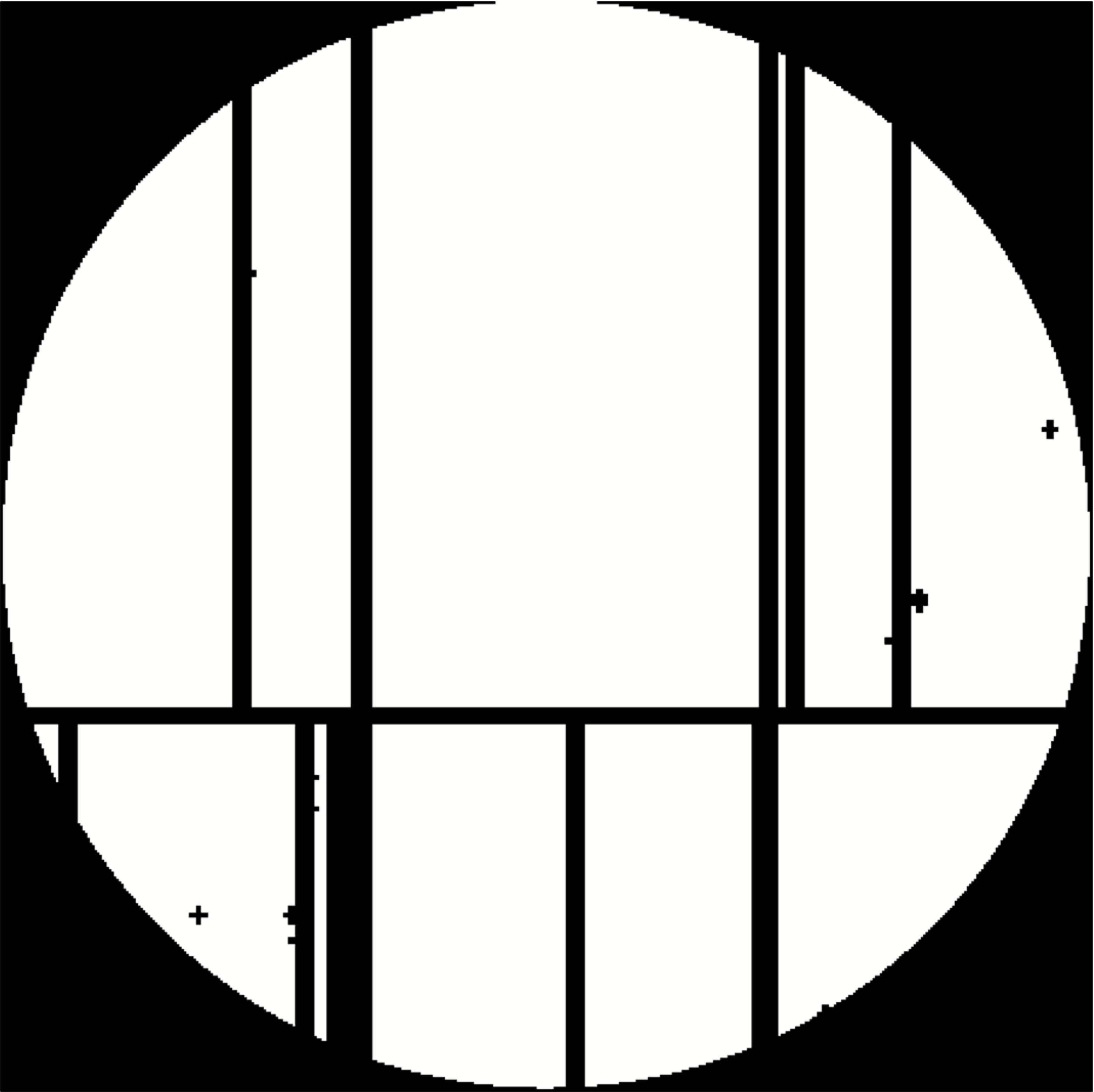
3.2.1 The masks

When modelling the bad pixel obscuration we must make a choice of the pixel size of our masks and model images. In order to accurately 1) map the bad pixels and 2) match the spectrum extraction region (Section 2.2) we adopted the smallest useful pixel size of (0.05 arcsec)², which is the size of a single pixel in the internal XMM-Newton detector focal plane coordinate system. This oversamples the physical EPIC-pn pixel by a factor of 82 $\times$ 82.

We utilised the eexpmap routine of SAS for creating the spatial masks of the bad pixels. While we are not interested in the exposure maps as such (which this tool is designed to produce), this tool anyhow provides a practical way of carrying out our task in hand. The idea is that bad pixels are traced by zero values in the exposure maps. In order to avoid possible complications arising when projecting the data from the detector plane (where the data are observed) to the more convenient sky coordinate system preferred by general users, we produced our bad pixel masks in the detector coordinate system.

We thus produced pn images in detector coordinates with a pixel size of 0.05 arcsec and used those as arguments for the imageset parameter when running eexpmap. We used attrebin=0.021 (arcsec) to make sure that if the attitude shifts by more than half the pixel size of 0.05 arcsec the translation between detector and sky coordinates is recalculated. We turned the resulting exposure maps into bad pixel masks by setting all pixels with zero exposure time as zero, while all other pixel values were set to unity (see Fig. 2).

3.2.2 The model images

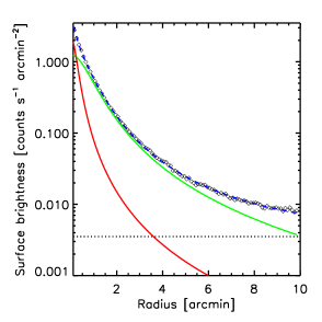
We base the synthetic pn model images on the surface brightness profile models obtained by fitting the MOS2 imaging data of a given cluster. We divided the raw count images by the exposure map to obtain vignetting-corrected count rate maps. Using those we accumulated the total count rate in co-centric annuli centered at the same point (the X-ray peak) as the spectrum extraction region (see Section 2.2) except that we ignored the bad pixels and brightest point sources. We divided the count rates with the area covered by the used pixels in a given annulus to obtain surface brightness profile. The background is defined as the constant surface brightness level at larger radii. We fitted the profiles with a single- $\beta$ or double- $\beta$ model

I(r)=I_{0,1}\times\left[1+{\left(\frac{r}{r_{\mathrm{core,1}}}\right)}^{2}\right]^{(-3\beta+\frac{1}{2})}+I_{0,2}\times\left[1+{\left(\frac{r}{r_{\mathrm{core,2}}}\right)}^{2}\right]^{(-3\beta+\frac{1}{2})}+bkg,

(2)

where r is the projected radius and bkg is the constant background (see Table 2 and Fig. 2)

Table 2: Best-fit surface brightness profile model parameters

cluster	I_0,1	r_core,1	I_0,2	r_core,2	$\beta$
	c s^-1 arcmin^-2	arcmin	c s^-1 arcmin^-2	arcmin
A85	0.32	1.6	1.7	0.31	0.53
A401	0.09	4.4	0.16	2.0	0.89
A478	0.88	1.2	2.3	0.30	0.65
A644	0.11	3.3	0.35	1.4	0.81
A754	0.02	11.2	0.13	2.4	0.64
A1650	0.13	2.9	0.52	0.82	0.91
A1651	0.14	2.9	0.31	1.1	0.90
A1795	0.27	1.7	2.0	0.54	0.59
A2029	1.3	0.95	2.3	0.27	0.58
A2142	0.43	1.2	0.55	0.60	0.53
A2244	0.40	1.2	0.28	0.33	0.66
A2319	0.15	2.7	0.23	1.2	0.49
A3112	0.48	1.1	2.5	0.24	0.65
A3391	0.04	4.4	0.04	1.1	0.74
A3558	0.07	7.3	0.19	1.6	1.1
A3571	0.26	3.1	0.28	0.77	0.60
A3827	0.07	4.0	0.20	1.6	1.0
Coma	0.14	7.5	—	—	0.51
CygA	3.5	0.30	—	—	0.51
Ophiuchus	0.47	4.1	1.0	0.46	0.59
PKS0745	0.49	1.2	3.2	0.39	0.68
Triangulum	0.06	8.4	0.23	2.7	0.77
ZwCl1215	0.07	3.8	0.05	1.5	0.82

The best-fit parameters for the $\beta$ model (Eq. 2) obtained by fitting the MOS2 data.

We then simulated an unobscured image of a given cluster using the surface brightness profile model obtained above (see Fig. 2). As in the case of the bad pixel masks (see Section 3.2.1) we produced the cluster images in the detector coordinate system using a pixel size of 0.05 arcsec. The synthetic image has identical attitude and offset between the cluster and FOV centers to those of the observational pn image and the mask image. The synthetic image yields the model count rate $CR(model,full)$ from the unobscured full central r=6 arcmin region of a given cluster.

The real galaxy clusters have a varying degree of deviations from the azimuthal symmetry we assumed when modelling the clusters. We essentially interpolate the surface brightness model to estimate the lost flux at the locations of the bad pixels. Given the random nature of the deviations from the symmetry we do not expect a significant bias in our modelling. This may cause some scatter between the modelled and arfgen - estimated fluxes which will manifest itself in our results.

3.3 Results

We then multiplied the model images with the masks in order to model the effect of the bad pixel/CCD gap obscuration. Using the mask-filtered images we then obtained the model count rate $CR(model,unobsc)$ in the surviving unobscured region. We then calculated the “true” flux reduction factor, i.e. the “true” effective area re-scaling factor

R_{model}=CR(model,unobsc)/CR(model,full)

(3)

for each observation. We then compared these with the effective area re-scaling factors R_image (Eq. 1) produced with arfgen using the observational data (see Section 3.1). The comparison yielded the following results for the central r = 6 arcmin regions of the EPIC FOV using SAS 18.0.0. (see Fig. 3 and Table 1).

•

On average, the flux reduction fraction as given by 1) the simulations (in detector coordinate system with a pixel size of 0.05 arcsec) and by 2) arfgen on the observational data (in sky coordinates with bad pixel resolution of 2 arcsec) differ by $\approx$ 0.03%
•

In some individual cases the difference exceeds 1% (1.4% at the maximum). The standard deviation of the full sample is $\approx$ 0.7%.
•

The above results do not change significantly when improving the bad pixel resolution from the default 2 arcsec to 0.2 arcsec when running arfgen. Therefore we recommend to use the default value of 2 arcsec when analysing extended sources.

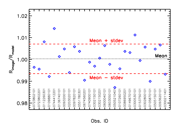
Figure 3: The ratios of the test values (R_image) to the model values (R_model) for each observation (blue diamonds), together with the sample average (denoted with black dotted line). Unity corresponds to a perfect match. The red dashed lines indicate the standard deviation.

4 Conclusions

We examined the accuracy of the recovery method of the EPIC flux obscured by the bad pixels in the central r = 6 arcmin region as implemented in SAS 18.0.0 i.e. using a supplementary raw count image for flux information. We used a sample of galaxy clusters for testing. We found that the accuracy of the recovered total flux is better than 0.1% on average while in individual cases the recovered flux may be uncertain by $\sim$ 1%.

Acknowledgements
The work is supported by the Horizon 2020 Framework Programme of the European Union Grant Agreement No. 871158. We acknowledge the support by the Estonian Research Council grants IUT40-2, PRG1006, and by the European Regional Development Fund (TK133). J.N. acknowledges ESAC Science Faculty support for a short visit when this work was initiated.