VEM and the Mesh

Abstract

In this work we report some results, obtained within the framework of the ERC Project CHANGE, on the impact on the performance of the virtual element method of the shape of the polygonal elements of the underlying mesh. More in detail, after reviewing the state of the art, we present a) an experimental analysis of the convergence of the VEM under condition violating the standard shape regularity assumptions, b) an analysis of the correlation between some mesh quality metrics and a set of different performance indexes, and c) a suitably designed mesh quality indicator, aimed at predicting the quality of the performance of the VEM on a given mesh.

1 Introduction

Geometrically complex domains are frequently encountered in mathematical models of real engineering applications. Their representation in some discrete form is a key aspect in the numerical approximation of the solutions of the partial differential equations (PDEs) describing such models and can be extremely difficult. The finite element method has been proved to be very successful as it allows the computational domains to be discretized by using triangular and quadrilateral meshes in 2D and tetrahedral and hexahedral meshes in 3D. Meshes with more complex elements, even admitting curved edges and faces, can be considered in the finite element formulation through reference elements and suitable remappings onto the problem space. To obtain accurate solutions, stringent constraints must be imposed, for example on the internal angles of the triangles and tetrahedra, thus requiring in extreme situations meshes with very small sized elements. To alleviate meshing issues, we can resort to numerical methods that are designed from the very beginning to provide arbitrary order of accuracy on more generally shaped elements. A class of methods with these features is the class of the so called polytopal element method, or PEM for short, that make it possible to numerically solve PDEs using polygonal and polyhedral grids.

The PEMs allow the user to incorporate complex geometric features at different scales without triggering mesh refinement, thus achieving high flexibility in the treatment of complex geometries. Moreover, nonconformal meshes can be treated in a straightforward way, by automatically including hanging nodes (i.e., T-junctions), and the design of refinement and coarsening algorithms is greatly simplified.

Such polytopal methods normally rely on a special design, as a straightforward generalization of the FEM is not possible because the finite element variational formulation requires an explicit knowledge of the basis functions. This requirement typically implies that such basis functions are elements of a subset of scalar and vector polynomials, and, as a consequence, the FEM is mostly restricted to meshes with elements having a simple geometrical shape, such as triangles or quadrilaterals.

The virtual element method (VEM) is a very successful example of PEM. The VEM formulation and implementation are based on suitable polynomial projections that we can always compute from the degrees of freedom of the basis functions. Since the explicit knowledge of the basis functions for the approximation space is not required, the method is dubbed as virtual. This fundamental property allows the virtual element to be formulated on meshes with elements having a very general geometric shapes.

The VEM was originally formulated in [5] as a conforming FEM for the Poisson problem by rewriting in a variational setting the nodal mimetic finite difference (MFD) method [27, 10, 14, 46] for solving diffusion problems on unstructured polygonal meshes. A survey on the MFD method can be found in the review paper [44] and the research monograph [11]. The VEM scheme inherits the flexibility of the MFD method with respect to the admissible meshes and this feature is well reflected in the many significant applications that have been developed so far, see, for example, [12, 18, 13, 20, 49, 53, 2, 9, 7, 8, 31, 54, 63, 35, 39, 19, 3, 34]. Since the VEM is a reformulation of the MFD method that generalizes the FEM to polytopal meshes as the other PEMs, it is clearly related with many other polytopal schemes. The connection between the VEM and finite elements on polygonal/polyhedral meshes is thoroughly investigated in [47, 33, 40], between VEM and discontinuous skeletal gradient discretizations in [40], and between the VEM and the BEM-based FEM method in [32]. The VEM has been extended to convection-reaction-diffusion problems with variable coefficients in [8]. The issue of preconditioning the VEM has been considered in [4, 22, 23, 30].

If on one hand, the VEM makes it possible to discretize a PDE on computational domains partitioned by a polytopal mesh, on the other hand this flexibility poses the fundamental question of what is a “good” polytopal mesh. All available theoretical and numerical results in the literature strongly support the fact that the quality of the mesh is crucial to determine the accuracy of the method and its effectiveness in solving problems on difficult geometries. This fact is not surprising as such dependence of the behavior of the numerical approximation in terms of accuracy, stability, and overall computational cost on the quality of the underlying mesh has been a very well known fact for decades in the finite element framework and has been formalized in concepts like mesh regularity, shape regularity, etc. However, the concept of shape regularity of triangular/tetrahedral and quadrangular/hexahedral meshes is well understood [38, 24, 57], but the characterization of a good polytopal mesh is still subject to ongoing research. Optimal convergence rates for the virtual element approximations of the Poisson equation were proved in $H^{1}$ and $L^{2}$ norms, see for instance [5, 1, 37, 17, 25, 26, 15]. These theoretical results involve an estimate of the approximation error, which is due to both analytical assumptions (interpolation and polynomial projections of the virtual element functions) and geometrical assumptions (the geometrical shape of the mesh elements).

A major point here is that the polytopal framework provides an enormous freedom to the possible geometric shapes of the mesh elements. This freedom makes it difficult to identify which geometric features may have a negative effect on the performance of the VEM. Various geometrical (or regularity) assumptions have been proposed to ensure that all elements of any mesh of a given mesh family in the refinement process are sufficiently regular. Many papers prove the convergence of the VEM and derive optimal error estimates under the assumption that the polygonal elements are star-shaped with respect to all the points in a disc whose diameter is comparable with the diameter of the elements itself. This assumption is combined with a second scaling assumption on the mesh elements in the sequence of refined meshes that is used in the numerical approximation. For example, we can assume that either the length of all the edges or the distance between any two vertices of a polygonal element scale comparably with the element diameter, or even weaker conditions. These assumptions guarantee the VEM convergence and optimal estimates of the approximation error with respect to different norms. However, as already observed from the very first papers, cf. [1], the VEM seems to maintain its optimal convergence rates also when we use mesh families that do not satisfy the usual geometrical assumptions. Since the VEM was proposed in 2013, many more examples have accumulate in the literature (some also reviewed in this chapter) that show that a virtual element solver on a simple model problem as the Poisson equation may still provide a very good behavior, even if all the theoretical conditions of the analysis are violated. Good behavior means that the VEM is convergent and the loss of accuracy is significant only when the degeneracy of the meshes becomes really extreme. This suggests that more permissive shape-regularity criteria should be devised so that the VEM can be considered as effective, and a lot of work still has to be carried out to identify the specific issues that may negatively affect its accuracy. Clearly, these points are also crucial to support the design of better polygonal meshing algorithm for the tessellation of computational domains.

Understanding the influence of the geometrical characteristics of the elements on the performance of the VEM and, more generally, of the PEM, is one of the goals that the unit based at the Istituto di Matematica Applicata e Tecnologie Informatiche del CNR is pursuing within the Advanced Grant Project New CHallenges in (adaptive) PDE solvers: the interplay of ANalysis and GEometry (CHANGE), whose final goal is the design of tools embracing geometry and analysis within a multi-level, multi-resolution paradigm. Indeed, a deeper understanding of such an interrelation can provide, on the one hand, the geometry processing community with information on the requirements to be incorporated into the meshing tools in order to generate “good” polytopal meshes, and, on the other hand, the mathematical community with possible new directions to pursue in the theoretical analysis of the VEM.

In Section 5 we review the main results of a recent work aimed at identifying the correlation between the performance of the virtual element method and a set of polygonal quality metrics. To this end, a systematic exploration was carried out to correlate the performance of the VEM and the geometric properties of the polygonal elements forming the mesh. In such study, the performance of the VEM is characterized by different “performance indexes”, including (but not limited to) the accuracy of the solution and the conditioning of the associated linear system. The quality “metrics” measuring the “goodness” of a mesh are built by considering several geometric properties of polygons (see subsection 5.1) from the simplest ones such as areas, angles, and edge length, to most complex ones as kernels, inscribed and circumscribed circles. The individual quality metrics of the polygonal elements of a mesh are combined in a single quality metric for the mesh itself by different aggregation strategies, such as minima, maxima, averages, worst case scenario and Euclidean norm. The numerical experiments to collect the results are performed on a family of parametric elements, which is designed to progressively stress one or more of the proposed geometric metrics, enriched with random polygons in order to avoid a bias in the study.

A second critical point developed in Section 6, is the connection between the performance of the method and how the regularity of the mesh refinements impacts on the approximation process. Note indeed that the way the geometric objects forming a mesh as edges and polygons (and faces and polytopal elements in 3D) scale is crucial in all possible geometric assumptions. It is a remarkable example shown in Section 4.1 that even the star-shaped assumption can be violated on a sequence of rectangular meshes (rectangular elements are star-shaped!) if the element aspect ratio scales badly when the mesh is refined. To study how the geometrical conditions that are found in the literature may really impact on the convergence and accuracy of the VEM, we gradually introduce several pathologies in the mesh datasets used in the numerical experiments. These datasets systematically violate all the geometrical assumptions, and enhance a correlation analysis between such assumptions and the VEM performance. As expected from other works in the literature, these numerical experiments confirm the remarkable robustness of the VEM as it fails only in very few and extreme situations and a good convergence rate is still visible in most examples. To quantify this correlation, we build an indicator that measure the violation of the geometrical assumptions. This indicator depends uniquely on the geometry of the mesh elements. A correspondence is visible between this indicator and the performance of the VEM on a given mesh, or mesh family, in terms of approximation error and convergence rate. This correspondence and such an indicator can be used to devise a strategy to evaluate if a given sequence of meshes is suited to the VEM, and possibly to predict the behaviour of the numerical discretization before applying the method.

The chapter is organized as follows. In Section 2, we present the VEM and the convergence results for the Poisson equation with Dirichlet boundary conditions. In Section 3.1, we detail the geometrical assumptions on the mesh elements that are used in the literature to guarantee the convergence of the VEM. In Section 3.2 we review the major theoretical results on the error analysis that are available in the virtual element literature, reporting the geometrical conditions assumed in each result. In Section 4.1, we present a number of datasets which do not satisfy these assumptions, and experimentally investigate the convergence of the VEM over them. In Section 5 we present the statistical analysis of the correlation between some notable mesh quality metrics and a selection of quantities measuring differents aspects of the performance of the VEM. In Section 6, we propose a mesh quality indicator to predict the behaviour of the VEM over a given dataset. In Section 7 we present the open source benchmarking software tools PEMesh [29], developed at IMATI.

2 Model problem

The elliptic model problem that we focus on in this paper is the Poisson equation with Dirichlet boundary conditions. In this section, we briefly review the strong and weak forms of the model equations and recall the formulation of its virtual element discretization.

The Poisson equation and its virtual element discretization. Let $\Omega$ be an open, bounded, connected subset of $\mathbbm{R}^{2}$ with polygonal boundary $\Gamma$. We consider the Poisson equation with homogeneous Dirichlet boundary conditions, whose strong form is:

$$-\Delta u=f \qquad\textrm{in~{}}\Omega,$$ (1)

$$u=0 \qquad\textrm{on~{}}\Gamma.$$ (2)

Remark that, while, for the sake of simplicity, we consider here homogeneous Dirichlet boundary conditions, the method that we are going to present also applies to the non homogeneous case, the extension being straightforward. The variational formulation of problem (1)-(2) takes the form: Find $u\in H^{1}_{0}(\Omega)$ such that

$$a(u,v)=F(v)\qquad\forall v\in H^{1}_{0}(\Omega),$$ (3)

with the bilinear form $a(\cdot,\cdot):H^{1}(\Omega)\times H^{1}(\Omega)\to\mathbbm{R}$ and the right-hand side linear functional $F:L^{2}(\Omega)\to\mathbbm{R}$ respectively defined as

$$a(u,v)=\int_{\Omega}\nabla u\cdot\nabla v\,d\mathbf{x}$$ (4)

and

$$F(v)=\int_{\Omega}fv\,d\mathbf{x},$$ (5)

where we implicitly assumed that $f\in L^{2}(\Omega)$. The well-posedness of the weak formulation (3) can be proven by applying the Lax-Milgram theorem [55, Section 2.7], thanks to the coercivity and continuity of the bilinear form $a(\cdot,\cdot)$, and to the continuity the linear functional $F(v)$.

We consider here the virtual element approximation of equation (3), mainly based on References [1, 5], which provides an optimal approximation on polygonal meshes when the diffusion coefficient is variable in space.

The discrete equation will take the form: Find $u_{h}\in V^{h}_{k}$ such that

$$a_{h}(u_{h},v_{h})=F_{h}(v_{h})\qquad v_{h}\in V^{h}_{k},$$ (6)

where $u_{h}$, $V^{h}_{k}$, $a_{h}(\cdot,\cdot)$, $F_{h}(\cdot)$ are the virtual element approximations of $u$, $H^{1}_{0}(\Omega)$, $a(\cdot,\cdot)$, and $F(\cdot)$. In the rest of this section we recall the construction of these mathematical objects.

Mesh notation. Let $\mathcal{T}=\{\Omega_{h}\}_{h\in\mathcal{H}}$ be a family of decompositions $\Omega_{h}$ of the computational domain $\Omega$ into a finite set of nonoverlapping polygonal elements $E$. Each of the members $\Omega_{h}$ of the family $\mathcal{T}$ will be referred to as the mesh. The mesh size $h$, which also serves as subindex, is the maximum of the diameters of the mesh elements, which is defined by $h_{E}=\sup_{\mathbf{x},\mathbf{y}\in E}\left|\mathbf{x}-\mathbf{y}\right|$. We assume that the mesh sizes of the mesh family $\mathcal{T}$ are in a countable subset $\mathcal{H}$ of the real line $(0,+\infty)$ having $0$ as its unique accumulation point. We let $\partial E$ denote the polygonal boundary of $E$, which we assume to be nonintersecting and formed by straight edges $e$. The center of gravity of $E$ will be denoted by $\mathbf{x}_{E}=(x_{E},y_{E})$ and its area by $\left|E\right|$. We denote the edge mid-point $\mathbf{x}_{e}=(x_{e},y_{e})$ and its lenght $\left|e\right|$, and, with a small abuse of notation, we write $e\in\partial E$ to indicate that edge $e$ is running throughout the set of edges forming the elemental boundary $\partial E$. In the next section we will discuss in detail the different assumptions on the mesh family $\mathcal{T}$, under which he convergence analysis of the VEM and the derivation of the error estimates in the $L^{2}$ and $H^{1}$ are carried out in the literature.

The virtual element spaces. Let $k\geq 1$ integer and $E\in\Omega_{h}$ a generic mesh element. We define the local virtual element space $V^{h}_{k}(E)$, following to the enhancement strategy proposed in [1]:

$$V^{h}_{k}(E)=\bigg{\{}\,v_{h}\in H^{1}(E)\,:\,{v_{h}}_{|{\partial E}}\in C^{0}(\partial E),\,{v_{h}}_{|{e}}\in\mathbbm{P}_{k}(e)\,\forall e\in\partial E,\,\\ \Delta v_{h}\in\mathbbm{P}_{k}(E),\,\textrm{and~{}}\\[2.5pt] \int_{E}(v_{h}-\Pi^{\nabla,E}_{k}v_{h})\,q\,dV=0\,\,\forall q\in\mathbbm{P}_{k}(E)\backslash\mathbbm{P}_{k-2}(E)\,\bigg{\}}.$$ (7)

Here, $\Pi^{\nabla,E}_{k}$ is the elliptic projection that will be discussed in the next section; $\mathbbm{P}_{k}(E)$ and $\mathbbm{P}_{k}(e)$ are the linear spaces of the polynomials of degree at most $k$, which are respectively defined over an element $E$ or an edge $e$ according to our notation; and $\mathbbm{P}_{k}(E)\backslash\mathbbm{P}_{k-2}(E)$ is the space of polynomials of degree equal to $k-1$ and $k$. By definition, the space $V^{h}_{k}(E)$ contains $\mathbbm{P}_{k}(E)$ and the global space $V^{h}_{k}$ is a conforming subspace of $H^{1}(\Omega)$. The global conforming virtual element space $V^{h}_{k}$ of order $k$ built on mesh $\Omega_{h}$ is obtained by gluing together the elemental approximation spaces, that is

$$V^{h}_{k}:=\Big{\{}\,v_{h}\in H^{1}_{0}(\Omega)\,:\,{v_{h}}_{|{E}}\in V^{h}_{k}(E)\,\,\,\forall E\in\Omega_{h}\,\Big{\}}.$$ (8)

On every mesh $\Omega_{h}$, given an integer $k\geq 0$, we also define the space of discontinuous piecewise polynomials of degree at most $k$, $\mathbbm{P}_{k}(\Omega_{h})$, whose elements are the functions $q$ such that ${q}_{|{E}}\in\mathbbm{P}_{k}(E)$ for every $E\in\Omega_{h}$.

The degrees of freedom. For each element $E$ and each virtual element function $v_{h}\in V^{h}_{k}(E)$, we consider the following set of degrees of freedom [5]:

(D1) for $k\geq 1$, the values of $v_{h}$ at the vertices of $E$;

(D2) for $k\geq 2$, the values of $v_{h}$ at the $k-1$ internal points of the $(k+1)$-point Gauss-Lobatto quadrature rule on every edge $e\in\partial E$.

(D3) for $k\geq 2$, the cell moments of $v_{h}$ of order up to $k-2$ on element $E$:

$$\frac{1}{\left|E\right|}\int_{E}v_{h}\,q\,dV\quad\forall q\in\mathbbm{P}_{k-2}(E).$$ (9)

It is possible to prove that this set of values is unisolvent in $V^{h}_{k}(E)$, cf. [5]; hence, every virtual element function is uniquely identified by it. The global degrees of freedom of a virtual element function in the space $V^{h}_{k}$ are given by collecting the elemental degrees of freedom (D1)-(D3) for all vertices, edges and elements. Their unisolvence in $V^{h}_{k}$ is an immediate consequence of their unisolvence in every elemental space $V^{h}_{k}(E)$.

The elliptic projection operators. The elliptic projection operator $\Pi^{\nabla,E}_{k}:H^{1}(E)\to\mathbbm{P}_{k}(E)$, whose definition is required in (7) and which will be instrumental in the definition of the bilinear form $a_{h}$ in the following, is given, for any $v_{h}\in V^{h}_{k}(E)$, by:

$$\int_{E}\nabla\Pi^{\nabla,E}_{k}v_{h}\cdot\nabla q\,dV =\int_{E}\nabla v_{h}\cdot\nabla q\,dV\quad\forall q\in\mathbbm{P}_{k}(E),$$ (10)

$$\int_{\partial E}\big{(}\Pi^{\nabla,E}_{k}v_{h}-v_{h}\big{)}\,dS =0.$$ (11)

Equation (11) allows us to remove the kernel of the gradient operator from the definition of $\Pi^{\nabla,E}_{k}$, so that the $k$-degree polynomial $\Pi^{\nabla,E}_{k}v_{h}$ is uniquely defined for every virtual element function $v_{h}\in V^{h}_{k}(E)$. Furthermore, projector $\Pi^{\nabla,E}_{k}$ is a polynomial-preserving operator, i.e., $\Pi^{\nabla,E}_{k}q=q$ for every $q\in\mathbbm{P}_{k}(E)$. By assembling elementwise contributions we define a global projection operator $\Pi^{\nabla}_{k}:H^{1}(\Omega)\to\mathbbm{P}_{k}(\Omega_{h})$, which is such that ${\Pi^{\nabla}_{k}v_{h}}_{|{E}}=\Pi^{\nabla,E}_{k}({v_{h}}_{|{E}})\ \forall E\in\Omega_{h}$. A key property of the elliptic projection operator is that the projection $\Pi^{\nabla,E}_{k}v_{h}$ of any virtual element function $v_{h}\in V^{h}_{k}(E)$ is computable from the degrees of freedom (D1)-(D3) of $v_{h}$ associated with element $E$.

Orthogonal projections. From the degrees of freedom of a virtual element function $v_{h}\in V^{h}_{k}(E)$ we can also compute the $L^{2}(E)$ orthogonal projections $\Pi^{0,E}_{k}v_{h}\in\mathbbm{P}_{k}(E)$, cf. [1]. In fact, $\Pi^{0,E}_{k}v_{h}$ of a function $v_{h}\in V^{h}_{k}(E)$ is, by definition, the solution of the variational problem:

$$\int_{E}\Pi^{0}_{k}v_{h}\,q\,dV=\int_{E}v_{h}\,q\,dV\qquad\forall q\in\mathbbm{P}_{k}(E).$$ (12)

The right-hand side is the integral of $v_{h}$ against the polynomial $q$, and, when $q$ is a polynomial of degree up to $k-2$, it is computable from the degrees of freedom (D3) of $v_{h}$. When $q$ is a polynomial of degree $k-1$ or $k$, it is computable from the moments of $\Pi^{\nabla,E}_{k}v_{h}$ , cf. (7). Clearly, the orthogonal projection $\Pi^{0,E}_{k-1}v_{h}$ is also computable. Also here we can define a global projection operator $\Pi^{0}_{k}:L^{2}(\Omega)\to\mathbbm{P}_{(}\Omega_{h})$, which projects the virtual element functions on the space of discontinuous polynomials of degree at most $k$ built on mesh $\Omega_{h}$. This operator is obtained by assembling the elemental $L^{2}$-orthogonal projections $\Pi^{0,E}_{k}v_{h}$ for all mesh elements $E$, that is ${\big{(}\Pi^{0}_{k}v_{h}\big{)}}_{|{E}}=\Pi^{0,E}_{k}({v_{h}}_{|{E}})$.

The virtual element bilinear forms. Taking advantage of the elliptic and orthogonal projectors we can now define the virtual element bilinear form $a_{h}(\cdot,\cdot):V^{h}_{k}\times V^{h}_{k}\to\mathbbm{R}$. We start by splitting the discrete bilinear form $a_{h}(\cdot,\cdot)$ as the sum of elemental contributions

$$a_{h}(u_{h},v_{h})=\sum_{E\in\Omega_{h}}a^{E}_{h}(u_{h},v_{h}),\quad$$ (13)

where the contribution of every element is a bilinear form $a^{E}_{h}(\cdot,\cdot):V^{h}_{k}(E)\times V^{h}_{k}(E)\to\mathbbm{R}$, approximating the corresponding elemental bilinear form $a^{E}(\cdot,\cdot):H^{1}(E)\times H^{1}(E)\to\mathbbm{R}$,

$$a^{E}(v,w)=\int_{E}\nabla v\cdot\nabla w\,dV,\quad\forall v,w\in H^{1}(E).$$

The bilinear form $a^{E}_{h}(\cdot,\cdot)$ on each element $E$ is itself split as the sum of two contributions: by

$$a^{E}_{h}(u_{h},v_{h})= \int_{E}\nabla\Pi^{\nabla,E}_{k}u_{h}\cdot\nabla\Pi^{\nabla,E}_{k}v_{h}\,dV+$$ (14)

$$S^{E}_{h}\Big{(}\big{(}I-\Pi^{\nabla,E}_{k}\big{)}u_{h},\big{(}I-\Pi^{\nabla,E}_{k}\big{)}v_{h}\Big{)}.$$

The stabilization term $S^{E}_{h}(\cdot,\cdot)$ in (14) can be any computable, symmetric, positive definite bilinear form defined on $V^{h}_{k}(E)$ such that

$$c_{*}a^{E}(v_{h},v_{h})\leq S^{E}_{h}(v_{h},v_{h})\leq c^{*}a^{E}(v_{h},v_{h})\quad\forall v_{h}\in V^{h}_{k}(E)\cap\textrm{ker}\big{(}\Pi^{\nabla,E}_{k}\big{)},$$ (15)

for two positive constants $c_{*}$ and $c^{*}$. Property (15) states that that $S^{E}_{h}(\cdot,\cdot)$ scales like $a^{E}(\cdot,\cdot)$ with respect to $h_{E}$. As $\Pi^{\nabla,E}_{k}$ is a polynomial preserving operator, the contribution of the stabilization term in the definition of $a^{E}_{h}(\cdot,\cdot)$ is zero one (or both) of the two entries is a polynomial of degree less than or equals to $k$.

Condition (15), is designed so that $a^{E}_{h}(\cdot,\cdot)$ satisfies the two following fundamental properties:

-

$k$-consistency: for all $v_{h}\in V^{h}_{k}(E)$ and for all $q\in\mathbbm{P}_{k}(E)$ it holds that

$$a^{E}_{h}(v_{h},q)=a^{E}(v_{h},q);$$ (16)

-

stability: there exist two positive constants $\alpha_{*},\,\alpha^{*}$, independent of $h$ and $E$, such that

$$\alpha_{*}a^{E}(v_{h},v_{h})\leq a^{E}_{h}(v_{h},v_{h})\leq\alpha^{*}a^{E}(v_{h},v_{h})\quad\forall v_{h}\in V^{h}_{k}(E).$$ (17)

In our implementation of the VEM, we consider the stabilization proposed in [48], that is we set:

$$S^{E}_{h}(v_{h},w_{h})=\sum_{i=1}^{N^{\textrm{dofs}}}\mathcal{A}^{E}_{ii}\textrm{DOF}_{i}(v_{h})\textrm{DOF}_{i}(w_{h}),$$ (18)

where $\mathcal{A}^{E}=\big{(}\mathcal{A}^{E}_{ij}\big{)}$ is the matrix stemming from the implementation of the first term in the bilinear form $a^{E}_{h}(\cdot,\cdot)$. More precisely, let $\phi_{i}$ be the $i$-th “canonical” basis functions generating the virtual element space, which is the function in $V^{h}_{k}(E)$ whose $i$-th degree of freedom for $i=1,\ldots,N^{\textrm{dofs}}$ (according to a suitable renumbering of the degrees of freedom in (D1), (D2), and (D3)), has value equal to $1$ and all other degrees of freedom are zero. The $i,j$-th entry of matrix $\mathcal{A}^{E}$ is given by

$$\mathcal{A}^{E}_{ij}:=a^{E}\big{(}\Pi^{\nabla,E}_{k}\phi_{i},\Pi^{\nabla,E}_{k}\phi_{j}\big{)}.$$ (19)

The stabilization in (18) is sometimes called the “D-recipe stabilization” in the virtual element literature. Observe that, if we instead replace $\mathcal{A}^{P}$ with the identity matrix, we get the the so called “dofi-dofi (dd) stabilization” originally proposed in [5]:

$$S^{E,\textrm{dd}}_{h}(v_{h},w_{h})=\sum_{i=1}^{N^{\textrm{dofs}}}\textrm{DOF}_{i}(v_{h})\textrm{DOF}_{i}(w_{h}).$$ (20)

The stabilization (20) underlies many of the convergence results available from the literature, which we briefly review in Section 3.2.

The virtual element forcing term. We approximate the right-hand side of (6), by splitting it into the sum of elemental contributions and approximating every local linear functional by replacing $v_{h}$ with $\Pi^{0,E}_{k}v_{h}$:

$$F(v_{h})=\sum_{E\in\Omega_{h}}\big{(}f,\Pi^{0,E}_{k}v_{h}\big{)}_{E}.\textrm{~{}~{}where~{}~{}}\big{(}f,\Pi^{0,E}_{k}v_{h}\big{)}_{E}=\int_{E}f\,\Pi^{0,E}_{k}v_{h}\,dV.$$ (21)

Approximation properties in the virtual element space. Under a suitable regularity assumption on the mesh family $\mathcal{T}$ (see assumption G3.1 in the next section), we can prove the following estimates on the projection and interpolation operators:

1. for every $s$ with $1\leq s\leq k+1$ and for every $w\in H^{s}(E)$ there exists a $w_{\pi}\in\mathbbm{P}_{k}(E)$ such that

   $$\left|w-w_{\pi}\right|_{0,E}+h_{E}\left|w-w_{\pi}\right|_{1,E}\leq Ch^{s}_{E}\left|w\right|_{s,E};$$ (22)

2. for every $s$ with $2\leq s\leq k+1$, for every $h$, for all $E\in\Omega_{h}$ and for every $w\in H^{s}(E)$ there exists a $w_{I}\in V^{h}_{k}(E)$ such that

   $$\left|w-w_{I}\right|_{0,E}+h_{E}\left|w-w_{I}\right|_{1,E}\leq Ch_{E}^{s}\left|w\right|_{s,E}.$$ (23)

Here, $C$ is a positive constant depending only on the polynomial degree $k$ and on some mesh regularity constants that we will present and discuss in the next section.

Main convergence properties. Thanks to the coercivity and continuity of the bilinear form $a_{h}(\cdot,\cdot)$, and to the continuity of the right-hand side linear functional $\big{(}f,\Pi^{0}_{k}\cdot\big{)}$, by applying the Lax-Milgram theorem [55, Section 2.7], we obtain the well-posedness of the discrete formulation (6).

Let then $u\in H^{k+1}(\Omega)$ be the solution to the variational problem (3) on a convex domain $\Omega$ with $f\in H^{k}(\Omega)$. Let $u_{h}\in V^{h}_{k}$ be the solution of the virtual element method (6) on every mesh of a mesh family $\mathcal{T}=\{\Omega_{h}\}$ satisfying a suitable set of mesh geometrical assumptions. Under suitable assumptions on the mesh familty $\mathcal{T}$, it is possible to prove that the following error estimates hold:

• the $H^{1}$-error estimate holds:

  $$||u-u_{h}||_{1,\Omega}\leq Ch^{k}\left(||u||_{k+1,\Omega}+|f|_{k,\Omega}\right);$$ (24)

• the $L^{2}$-error estimate holds:

  $$||u-u_{h}||_{0,\Omega}\leq Ch^{k+1}\left(||u||_{k+1,\Omega}+|f|_{k,\Omega}\right).$$ (25)

Constant $C$ in (24) and in (25) may depend on the stability constants $\alpha_{*}$ and $\alpha^{*}$, on mesh regularity constants which we will introduce in the next section, on the size of the computational domain $\left|\Omega\right|$, and on the approximation degree $k$. Constant $C$ is normally independent of $h$, but for the most extreme meshes it may depend on the ratio between the longest and shortest edge lenghts, cf. Section 3.2.

Finally, we note that the approximate solution $u_{h}$ is not explicitly known inside the elements. Consequently, in the numerical experiments of Section 4.2, we approximate the error in the $L^{2}$-norm as follows:

$$||u-u_{h}||_{0,\Omega}\approx||u-\Pi^{0}_{k}u_{h}||_{0,\Omega},$$

where $\Pi^{0}_{k}u_{h}$ is the global $L^{2}$-orthogonal projection of the virtual element approximation $u_{h}$ to $u$. On its turn, we approximate the error in the energy norm as follows:

$$|u-u_{h}|_{1,\Omega}\approx a_{h}(u_{I}-u_{h},u_{I}-u_{h})$$

where $u_{I}$ is the virtual element interpolant of the exact solution $u$.

In this work, we are interested in checking whether optimal convergence rates put forward by these estimates are maintained on different mesh families that may display some pathological situations. From a theoretical viewpoint, the convergence estimates hold under some constraints on the shapes of the elements forming the mesh, called mesh geometrical (or regularity) assumptions. We summarize the major findings from the literature in Section 3.2 and in the next sections we will investigate how breaking such constraints may affect these results.

3 State of the art

Various geometrical (or regularity) assumptions have been proposed in the literature to ensure that all elements of all meshes in a given mesh family in the refinement process are sufficiently regular. These assumptions guarantee the convergence of the VEM and optimal estimates of the approximation error with respect to different norms.
In this section, we overview the geometrical assumptions introduced in the VEM literature to guarantee the convergence of the method, and we provide a list of the main convergence results based on such assumptions.

3.1 Geometrical assumptions

We start by reviewing the geometrical assumptions appeared in the VEM literature since their definition in [5]. Note that these assumptions are defined for a single mesh $\Omega_{h}$, but the conditions contained in them are required to hold independently of the mesh size $h$. As a consequence, when an assumption is imposed to a mesh family $\mathcal{T}=\{\Omega_{h}\}_{h}$, it has to be verified simultaneously by every $\Omega_{h}\in\mathcal{T}$.

It is well-known from the FEM literature that the approximation properties of a method depend on specific assumptions on the geometry of the mesh elements. Classical examples of geometrical assumptions for a family of triangulations $\{\Omega_{h}\}_{h\to 0}$, are the ones introduced in [38] and [64], respectively:

$(a)$

Shape regularity condition: there exists a real number $\gamma\in(0,1)$, independent of $h$, such that for any triangle $E\in\Omega_{h}$ we have

$$r_{E}\geq\gamma h_{E},$$ (26)

being $h_{E}$ the longest edge in $E$ and $r_{E}$ its inradius;

$(b)$

Minimum angle condition: there exists an angle $\alpha_{0}>0$, independent of $h$, such that for any triangle $E\in\Omega_{h}$ we have

$$\alpha_{E}\geq\alpha_{0},$$ (27)

being $\alpha_{E}$ the minimal angle of $E$.

When we turn our focus on polygonal meshes, a preliminar consideration is needed on the definition of the polygonal elements. It is commonly accepted, even if not always explicitly specified, that a mesh $\Omega_{h}$ has to be made of a finite number of simple polygons, i.e. open simply connected sets whose boundary is a non-intersecting line made of a finite number of straight line segments.
The other regularity assumptions proposed in the VEM literature to ensure approximation properties have been deduced in analogy to the similar conditions developed for the FEMs. The main assumption, which systematically recurs in every VEM paper, is the so-called star-shapedness of the mesh elements.

Assumption G​ 3.1

there exists a real number $\rho\in(0,1)$, independent of $h$, such that every polygon $E\in\Omega_{h}$ is star-shaped with respect to a disc with radius

$$r_{E}\geq\rho h_{E}.$$

We denote $r_{E}$ the radius of the greatest possible inscribed disk in $E$ and star center the center of such disk, where it exists. We stress the fact that G1 does not accept polygons star-shaped with respect to a single point, as both $\rho$ and $h_{E}$ are greater than zero, and we conventionally say that $r_{E}=0$ if $E$ is not star-shaped.

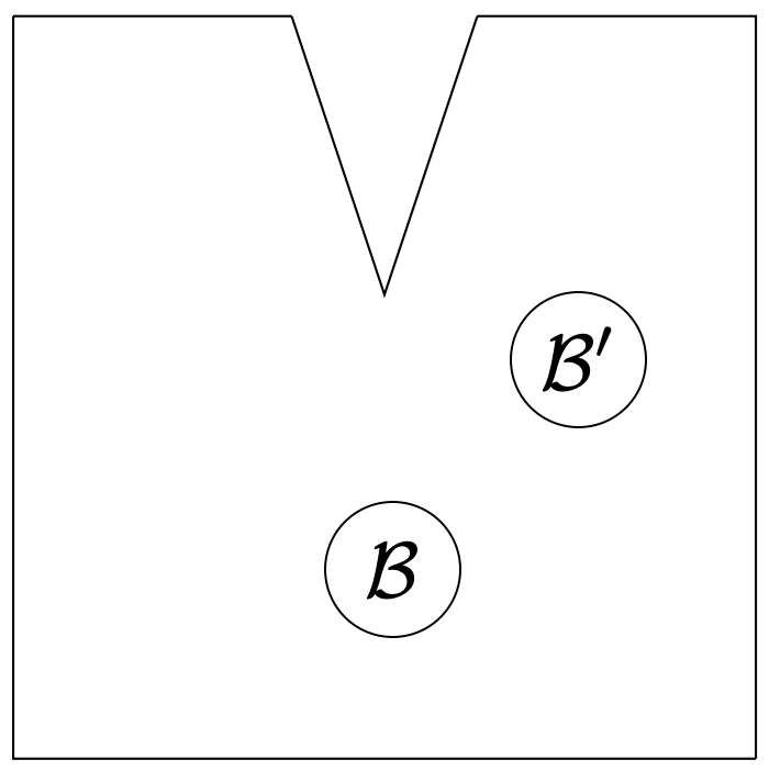
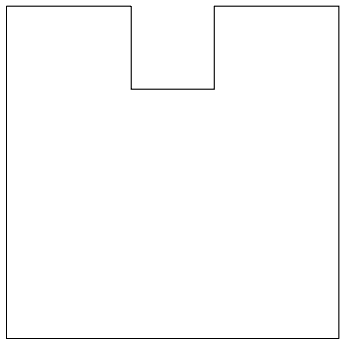
(a)	(b)

Figure 1: The element in (a) is star-shaped with respect to the disk $\mathcal{B}$ but not with respect to the disk $\mathcal{B}^{\prime}$, while the element in (b) is not star-shaped with respect to any disk.

Assumption G3.1 is nothing but the polygonal extension of the classical shape regularity condition for triangular meshes. In fact, any triangular element $E$ is star-shaped with respect to its maximum inscribed disk (the one with radius $r_{E}$) and the diameter $h_{E}$ coincides with its longest edge. Moreover, G3.1 can also be stated in the following weak form, as specified in [5] and more accurately in [25]:

Assumption G1-weak there exists a real number $\rho\in(0,1)$, independent of $h$, such that every polygon $E\in\Omega_{h}$ can be split into a finite number $N$ of disjoint polygonal subcells $E_{1},\dots,E_{N}$ where, for $j=1,\dots,N$,

$(a)$

element $E_{j}$ is star-shaped with respect to a disc with radius $r_{E_{j}}\geq\rho h_{E_{j}}$;

$(b)$

elements $E_{j}$ and $E_{j+1}$ share a common edge.

From a practical point of view, assumptions G3.1 and G1-weak are almost equivalent, and they are treated equivalently in all papers reviewed in Section 3.2.

Assumption G3.1 plays a key role in most of the theoretical results regarding polygonal methods. It is needed by the Bramble-Hilbert lemma [55], an important result on polynomial approximation that is often used for building approximation estimates, and also by the following lemma.

Lemma 3.2

If a mesh $\Omega_{h}$ satisfies Assumption G3.1 then for all polygons $E\in\Omega_{h}$ there exists a mapping $F:\mathcal{B}_{1}\to E$, with the Jacobian $J$ of $F$ satisfying

$$||J||_{2}\lesssim h,\qquad|\det(J)|\lesssim h^{2}\qquad\textit{and}\qquad||J^{-1}||_{2}\lesssim h^{-1},$$ (28)

and, for a sufficiently regular $u$, the following relations hold

$$||u||_{0,E}\simeq h_{E}||u\circ F||_{0,\mathcal{B}_{1}}, ||u||_{0,\partial E}\simeq h_{E}^{1/2}||u\circ F||_{0,\partial\mathcal{B}_{1}},$$

$$|u|_{1,E}\simeq|u\circ F|_{1,\mathcal{B}_{1}}, |u|_{1/2,\partial E}\simeq|u\circ F|_{1/2,\partial\mathcal{B}_{1}},$$

where all the implicit constants only depend on the constant $\rho$ from G3.1.

Thanks to the relations in Lemma 3.2, inequalities that we have on the unit circle $\mathcal{B}_{1}$, such as the Poincaré inequality or the trace inequalities, may be transferred to the polygon $E$ by a “scaling” argument.

In the very first VEM paper [5], where the method was introduced, Assumption G3.1 was followed by another condition on the maximum point-to-point distance.

Assumption G2-strong there exists a real number $\rho\in(0,1)$, independent of $h$, such that for every polygon $E\in\Omega_{h}$, the the distance $d_{i,j}$ between any two vertices $v_{i},v_{j}$ of $E$ satisfies

$$d_{i,j}\geq\rho h_{E}.$$

In fact, Assumption G2-strong was soon replaced in the following works [1], [17] and [25] by a weaker condition on the length of the elemental edges. This new version allows, for example, the existence of four-sided polygons with equal edges but one diagonal much smaller than the other.

Assumption G​ 3.3

there exists a real number $\rho\in(0,1)$, independent of $h$, such that for every polygon $E\in\Omega_{h}$, the length $\left|e\right|$ of every edge $e\in\partial E$ satisfies

$$\left|e\right|\geq\rho h_{E}.$$

The Authors consider a single constant $\rho$ for both Assumption G3.1 and G3.3 and refer to it as the mesh regularity constant or parameter.
Under Assumption G1-weak and G3.3, it can be proved [25] that the simplicial triangulation of $E$ determined by the star-centers of $E_{1},\dots,E_{N}$ satisfies the shape regularity and the minimum angle conditions. The same holds under Assumptions G3.1 and G3.3, as a special case of the previous statement. Moreover, Assumption G3.3 implies that for $1\leq j,k\leq N$ it holds ${h_{E_{j}}}/{h_{E_{k}}}\leq\rho^{-|j-k|}$.
As already mentioned in the very first papers, these assumptions are more restrictive than necessary, but at the same time they allow the VEM to work on very general meshes. For example, Ahmad et al. in [1] state that:

“Actually, we could get away with even more general assumptions, but then it would be long and boring to make precise (among many possible crazy decompositions that nobody will ever use) the ones that are allowed and the ones that are not.”

In the subsequent papers [17] and [26] assumption G3.1 is preserved, but assumption G3.3 is substituted by the alternative version:

Assumption G​ 3.4

There exists a positive integer $N$, independent of $h$, such that the number of edges of every polygon $E\in\Omega_{h}$ is (uniformly) bounded by $N$.

The Authors show how assumption G3.3 implies assumption G3.4, but assumption G3.4 is weaker than assumption G3.3, as it allows for edges arbitrarily small with respect to $h_{E}$. Both combinations G3.1+G3.3 and G3.1+G3.4 imply that the number of vertices of $E$ and the minimum angle of the simplicial triangulation of $E$ obtained by connecting all the vertices of $E$ to its star-center, are controlled by the constant $\rho$.

Another step forward in the refinement of the geometrical assumptions was made by Beirão Da Veiga et al. in [15]. Besides assuming G3.1, the Authors imagine to ”unwrap” the boundary $\partial E$ of each element $E\in\Omega_{h}$ onto an interval of the real line, obtaining a one-dimensional mesh $\mathcal{I}_{E}$. The mesh $\mathcal{I}_{E}$ can be subdivided into a number of disjoint sub-meshes $\mathcal{I}_{E}^{1},\ldots,\mathcal{I}_{E}^{N}$, corresponding to the edges of $E$. Then, the following condition is assumed.

Assumption G​ 3.5

There exists a real number $\delta>0$, independent of $h$, such that for every polygon $E\in\Omega_{h}$:

$(a)$

the one-dimensional mesh $\mathcal{I}_{E}$ can be subdivided into a finite number $N$ of disjoint sub-meshes $\mathcal{I}_{E}^{1},\ldots,\mathcal{I}_{E}^{N}$;

$(b)$

for each sub-mesh $\mathcal{I}_{E}^{i}$, $i=1,\ldots,N$, it holds that

$$\frac{\max_{e\in\mathcal{I}_{E}^{i}}|e|}{\min_{e\in\mathcal{I}_{E}^{i}}|e|}\leq\delta.$$

Each polygon $E$ corresponds to a one-dimensional mesh $\mathcal{I}_{E}$, but a sub-mesh $\mathcal{I}_{E}^{i}\subset\mathcal{I}_{E}$ might contain more than one edge of $E$, cf. Fig. 2. Therefore assumption G3.5 does not require a uniform bound on the number of edges in each element and does not exclude the presence of small edges. Mesh families created by agglomeration, cracking, gluing, etc.. of existing meshes are admissible according to G3.5.

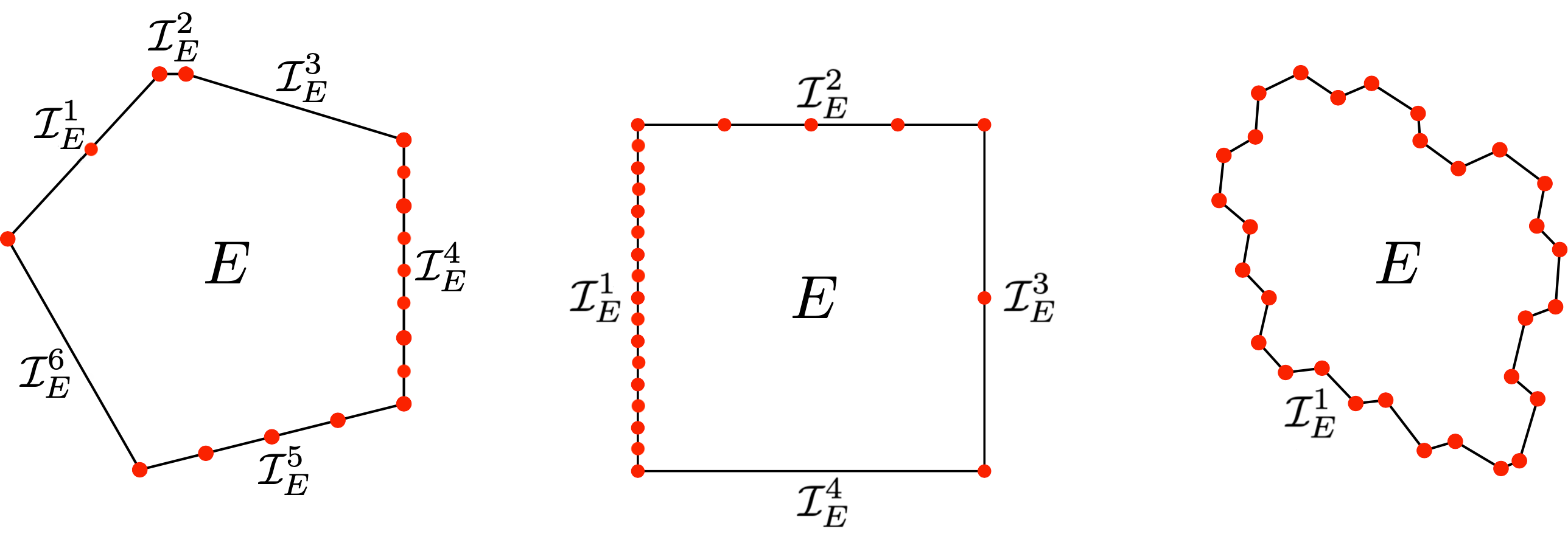
Figure 2: Examples of admissible elements according to assumption G3.5. Red dots indicate the vertices of the element.

As we will see in the next section, possible assumption pairs requested in the literature to guarantee the convergence of the VEM are given by combining G3.1 (or, equivalently, G1-weak) with either G2-strong, G3.3, G3.4 or G3.5.

Last, we report a condition (together with its weaker version) that appears in the literature related to the non-conforming version of the VEM, which we do not cover in this work. It is defined for instance in [21], but it can also be found under the name of local quasi-uniformity.

Assumption G​ 3.6

there exists a real number $\gamma\in(0,1)$, independent of $h$, such that for every polygon $E\in\Omega_{h}$, for all $e,e^{\prime}$ adjacent edges of $E$ it holds that

$$\frac{1}{\gamma}\leq\frac{|e|}{|e^{\prime}|}\leq\gamma.$$

In this case, the polygonal elements of the mesh are allowed to have a very large number of very small edges, provided that every two consecutive edges scale proportionally. This assumption also has a weak version, in which we essentially ask that, for every $E\in\Omega_{h}$, a part of $\partial E$ satisfies G3.6 and the remaining part satisfies G3.4.

Assumption G5-weak there exist a real number $\gamma\in(0,1)$ and a positive integer $N$, both independent of $h$, such that for every polygon $E\in\Omega_{h}$, the set $\mathcal{E}_{E}$ of the edges of $E$ can be split as $\mathcal{E}_{E}=\mathcal{E}_{E}^{1}\cup\mathcal{E}_{E}^{2}$, where $\mathcal{E}_{E}^{1}$ and $\mathcal{E}_{E}^{2}$ are such that

-

for any pair of adjacent edges $e,e^{\prime}\in\mathcal{E}_{E}$ with $e\in\mathcal{E}_{E}^{1}$, the inequality holds

$$\frac{1}{\gamma}\leq\frac{|e|}{|e^{\prime}|}\leq\gamma;$$

-

$\mathcal{E}_{E}^{2}$ contains at most $N$ edges.

Assumption G5-weak allows for situations where a large number of small edges coexists with some large edges. We can think of families of meshes for which such an assumption is not satisfied, but they would be extremely pathological. Assumptions G5 and G5-weak are here reported for the sake of completeness but are not considered in the analysis of the following sections, as they refer to a different context.

3.2 Convergence results in the VEM literature

In this section, we briefly overview the literature on the main results of the convergence analysis of the VEM method. For each article, we explicitly report (if available) the theoretical results and highlight the geometric assumptions used, reporting the abstract energy error, the $H^{1}$ error estimate, and the $L^{2}$ error. For a greater uniformity of the presentation with the rest of the chapter, we have slightly modified some notations and introduced minimal variations to some statements of the theorems.

“Basic Principles of Virtual Elements Methods” [5]
This is the paper in which the VEM method was introduced and defined. In the original formulation, the paper introduced the regular conforming virtual element space. For simplicity and with a small abuse of notation, the regular conforming virtual element space is denoted by $V^{h}_{k}$ as in (8) and (7):

$$V^{h}_{k}:= \{v_{h}\in H^{1}(\Omega):\ {v_{h}}_{|{E}}\in V^{h}_{k}(E)\ \forall E\in\Omega_{h}\},$$ (29a)

where

$$V^{h}_{k}(E):=\{v_{h}\in H^{1}(E):\ {v_{h}}_{|{\partial E}}\in C^{0}(\partial E),\ {v_{h}}_{|{e}}\in\mathbbm{P}_{k}(e)\ \forall e\in\partial E,$$ (29b)

$$\text{and }\ \Delta v_{h}\in\mathbbm{P}_{k-2}(E)\},$$

and the dofi-dofi formulation $S^{E,\textrm{dd}}_{h}$ defined in (20) is used for the stabilization bilinear form.
There, the authors introduced the concept of simple polygon and the geometric regularity assumptions G3.1 and G3.3 - strong. The following statement on the convergence of VEM in the energy norm is general and largely used in the VEM literature, even if not explicitly stated in [5]. To this purpose, for functions $v\in H^{1}(\Omega_{h})$ the broken $H^{1}$-seminorm is defined as follows:

$$|v|_{h,1}:=\left(\sum_{E\in\Omega_{h}}|\nabla v|_{0,E}^{2}\right)^{1/2}.$$ (30)

Theorem 3.1 (abstract energy error)

Under the k-consistency and stability assumptions defined in Subsection 2, cf. (16) and (17), the discrete problem has a unique solution $u_{h}$. Moreover, for every approximation $u_{I}\in V^{h}_{k}$ of $u$ and every approximation $u_{\pi}$ of $u$ that is piecewise in $\mathbbm{P}_{k}(\Omega_{h})$, we have

$$|u-u_{h}|_{1,\Omega}\leq C(|u-u_{I}|_{1,\Omega}+|u-u_{\pi}|_{h,1}+\mathfrak{F}_{h}),$$ (31)

where $C$ is a constant depending only on $\alpha_{*}$ and $\alpha^{*}$ (the constants in (17)), and, for any $h$, $\mathfrak{F}_{h}=|f-f_{h}|_{{V^{h}_{k}}^{\prime}}$ is the smallest constant such that

$$(f,v)-\langle f_{h}-f,v\rangle\leq\mathfrak{F}_{h}|f|_{1}\qquad\forall v\in V^{h}_{k}.$$

In [5] it was claimed that it is possible to estimate the convergence rate in terms of the $L^{2}$ error using duality argument techniques.

“Equivalent projectors for virtual element methods” [1]
In [1], the enhanced VEM space (7) adopted in this chapter replaces $V^{h}_{k}(E)$ (in [1] the enhanced VEM space is named “modified VEM space”). This paper uses the dofi-dofi stabilization. Under the geometrical assumptions G3.1 and G3.3, the paper provides an explicit estimation of $H^{1}$ and $L^{2}$ errors and introduces the Theorem 3.1 for the abstract energy error.

Theorem 3.2 ($H^{1}$ error estimate)

Assuming G3.1, G3.3, let the right-hand side $f$ belong to $H^{k-1}(\Omega)$, and that the exact solution $u$ belong to $H^{k+1}(\Omega)$. Then

$$||u-u_{h}||_{1,\Omega}\leq C|h|^{k}|u|_{k+1,\Omega}$$ (32)

with $C$ a positive constant independent of $h$.

Theorem 3.3 ($L^{2}$ error estimate)

Assuming G3.1, G3.3 and with $\Omega$ convex, let the right-hand side $f$ belong to $H^{k}(\Omega)$, and that the exact solution $u$ belong to $H^{k+1}(\Omega)$. Then

$$||u-u_{h}||_{0,\Omega}+|h|||u-u_{h}||_{1,\Omega}\leq C|h|^{k+1}|u|_{k+1,\Omega},$$ (33)

with $C$ a constant independent of $h$.

“Stability analysis for the virtual element method” [17]
This contribution deals with the regular conforming VEM space (29) defined in [5]. The paper [17] provides a new estimation of the abstract energy error and analyses the $H^{1}$ error with respect to two different stabilization techniques. Moreover, new analytical assumptions on the bilinear form $a_{h}(\cdot,\cdot)$ to replace (17) are introduced:

$$a^{E}_{h}(v_{h},v_{h}) \leq C_{1}(E)|||v_{h}|||_{{E}}^{2},\text{ for all }v_{h}\in V^{h}_{k}(E);$$ (34a)

$$|||q|||_{{E}}^{2} \leq C_{2}(E)a^{E}_{h}(q,q),\text{ for all }q\in\mathbbm{P}_{k}(E),$$ (34b)

being $|||\cdot|||_{{E}}$ a discrete semi-norm induced by the stability term and $C_{1}(E),C_{2}(E)$ positive constants which depend on the shape and possibly on the size of $E$. In this paper, the estimate is necessary for the polynomials $q\in\mathbbm{P}_{k}(E)$ only, while in the standard analysis in [5] a kind of bound (34a)(b) was required for every $v_{h}\in V^{h}_{k}(E)$. Thus, even when $C_{1}(E)$ and $C_{2}(E)$ can be chosen independent of $E$, on $V^{h}_{k}(E)$ the semi-norm induced by the stabilization term may be stronger than the energy $a^{E}_{h}(\cdot,\cdot)^{1/2}$.

Theorem 3.4 (abstract energy error)

Under the stability assumptions (34a), let the continuous solution $u$ of the problem satisfy ${u}_{|{E}}\in\mathcal{V}_{E}$ for all $E\in\Omega_{h}$, where $\mathcal{V}_{E}\subseteq V^{h}_{k}(E)$ is a subspace of sufficiently regular functions. Then, for every $u_{I}\in V^{h}_{k}$ and for every $u_{\pi}$ such that $u_{\pi|E}\in\mathbbm{P}_{k}(E)$, the discrete solution $u_{h}$ satisfies

$$|u-u_{h}|_{1,\Omega}\lesssim C_{\text{err}}(h)\ (\mathfrak{Fs}_{h}+|||u-u_{I}|||+|||u-u_{\pi}|||+|u-u_{I}|_{1,\Omega}+|u-u_{\pi}|_{h,1}),$$ (35)

where the constant $C_{\text{err}}(h)$ is given by

$$C_{\text{err}}(h)=\max\left\{1,\,\tilde{C}(h)C_{1}(h),\tilde{C}(h)^{3/2}\sqrt{C^{*}(h)C_{1}(h)}\right\}.$$

From the previous theorem, the following quantities are derived from the constants in (34a):

$$\tilde{C}(h)=\max_{E\in\Omega_{h}}\{1,\,C_{2}(E)\},\quad C_{1}(h)=\max_{E\in\Omega_{h}}\{C_{1}(E)\},$$

$$C^{*}(h)=\frac{1}{2}\max_{E\in\Omega_{h}}\{\min\{1,C_{2}(E)^{-1}\}\}.$$

In [17] the stability term $S^{E}_{h}(\cdot,\cdot)$ is considered as the combination of two contributions: the first, $S_{h}^{\partial E}$, related to the boundary degrees of freedom; the second, $S_{h}^{oE}$, related to the internal degrees of freedom. In the following statements, we restrict the analysis to $S_{h}^{\partial E}$ without losing generality. In this case,$S_{h}^{\partial E}$ is expressed in the dofi-dofi form $S_{h}^{\partial E,\textrm{dd}}$ defined in (20), or in the trace form introduced in [63]:

$$S_{h}^{\partial E,\textrm{tr}}(v_{h},w_{h})=h_{E}\int_{\partial E}\partial_{s}v_{h}\partial_{s}w_{h}ds,$$ (36)

where $\partial_{s}v_{h}$ denotes the tangential derivative of $v_{h}$ along $\partial E$.

Theorem 3.5 ($H^{1}$ error estimate with dofi-dofi stabilization)

Assuming G3.1, G3.4, let $u\in H^{s}(\Omega)$, $s>1$, be the solution of the problem with $S^{E}_{h}=S_{h}^{\partial E,\textrm{dd}}$. Let $u_{h}$ be the solution of the discrete problem, then it holds

$$||u-u_{h}||_{1,\Omega}\lesssim C(h)h^{s-1}|u|_{s,\Omega}\quad 1<s\leq k+1,$$ (37)

with

$$C(h)=\max_{E\in\Omega_{h}}(\log(1+h_{E}/h_{m}(E))),$$

where $h_{m}(E)$ denotes the length of the smallest edge of $E$.

Corollary 3.7

Assuming G3.1 and G3.3 instead, then $c(h)\lesssim 1$ and therefore

$$||u-u_{h}||_{1,\Omega}\lesssim h^{s-1}|u|_{s,\Omega}\qquad 1<s\leq k+1.$$

Theorem 3.6 ($H^{1}$ error estimate with trace stabilization)

Under Assumption G3.1, let $u\in H^{s}(\Omega)$, $s>3/2$ be the solution of the problem with $S^{E}_{h}=S_{h}^{\partial E,\textrm{tr}}$. Let $u_{h}$ be the solution of the discrete problem, then it holds

$$||u-u_{h}||_{1,\Omega}\lesssim h^{s-1}|u|_{s,\Omega}\quad 3/2<s\leq k+1.$$ (38)

“Some Estimates for Virtual Element Methods” [25]
In [25], the enhanced VEM space is defined as in the following:

$$\begin{split}V^{h}_{k}(E):=\big{\{}v_{h}\in H^{1}(E):\ &{v_{h}}_{|{\partial E}}\in\mathbbm{P}_{k}(\partial E),\\ &\exists\,q_{v_{h}}(=-\Delta v_{h})\in\mathbbm{P}_{k}(E)\text{~{}such~{}that~{}}\\ &\int_{E}\nabla v_{h}\cdot\nabla w_{h}\,d\mathbf{x}=\int_{E}q_{v_{h}}w_{h}\,d\mathbf{x}\quad\forall w_{h}\in H^{1}_{0}(E),\\ &\text{~{}and~{}}\Pi_{k}^{0,E}v_{h}-\Pi_{k}^{\nabla,E}v_{h}\in\mathbbm{P}_{k-2}(E)\big{\}}.\end{split}$$ (39)

i.e., in a slightly different but equivalent way than (7). In this work, the Authors consider different types of stabilization, but the convergence results are independent of $S^{E}_{h}$. The geometrical assumptions used in [25] are G3.1 and G3.3.

Theorem 3.7 (abstract energy error)

Assuming G3.1, G3.3, if $f\in H^{s-1}(\Omega)$ for $1\leq s\leq k$, then there exists a positive constant $C$ depending only on $k$ and $\rho$ from G3.1 such that

$$|u-u_{h}|_{1,\Omega}\leq C(\inf_{v\in V^{h}_{k}}|u-v|_{1,\Omega}+\inf_{w\in\mathbbm{P}_{k}(\Omega_{h})}|u-w|_{h,1}+h^{s}|f|_{s-1,\Omega}).$$ (40)

Theorem 3.8 ($H^{1}$ error estimate)

Assuming G3.1, G3.3, if $u\in H^{s+1}(\Omega)$ for $1\leq s\leq k$, then there exists positive constants $C_{1}$, $C_{2}$ depending only on $k$ and $\rho$ from G3.1 such that

$$|u-u_{h}|_{1,\Omega}+|u-\Pi^{\nabla}_{k}u_{h}|_{h,1}\leq C_{1}h^{s}|u|_{s+1,\Omega}.$$ (41)

Theorem 3.9 ($L^{2}$ error estimate)

Assuming G3.1, G3.3, with $\Omega$ convex, if $u\in H^{s+1}(\Omega)$ for for $1\leq s\leq k$, then there exists a positive constant $C$ depending only on $\Omega$, $k$ and $\rho$ from G3.1 such that

$$||u-u_{h}||_{0,\Omega}\leq Ch^{s+1}|u|_{s+1,\Omega}.$$ (42)

“Virtual element methods on meshes with small edges or faces” [26]
In this paper, error estimates of the VEM are yield for polygonal or polyhedral meshes possibly equipped with small edges $(d=2)$ or faces $(d=3)$. In this case, the VEM space is formulated as (39) (i.e., the so-called enhanced space). The local stabilizing bilinear form is considered in both the dofi-dofi ($S^{E,\textrm{dd}}_{h}$) and in the trace ($S^{E,\textrm{tr}}_{h}$of (36)) formulations. The Authors introduce also the constants:

$$\mathcal{H}:=\sup_{E\in\Omega_{h}}\left(\frac{\max_{e\in\partial E}h_{e}}{\min_{e\in\partial E}h_{e}}\right),\qquad\alpha_{h}:=\begin{cases}\ln\left(1+\mathcal{H}\right)&\mbox{~{}with }S^{E,\textrm{dd}}_{h}\\ 1&\mbox{~{}with }S^{E,\textrm{tr}}_{h}\end{cases}$$ (43)

The geometrical assumptions considered in this work are G3.1 and G3.4. In particular, a mesh-dependent energy norm $||\cdot||_{h}:=\sqrt{a_{h}(\cdot,\cdot)}$ and a functional $\Xi_{h}:V^{h}_{k}\to\mathbbm{P}_{k}(\Omega_{h})$ are introduced. The function $\Xi_{h}$ is defined as:

$$\Xi_{h}=\begin{cases}\Pi^{0}_{1}&\mbox{ if }k=1,2\\ \Pi^{0}_{k-1}&\mbox{ if }k\geq 3.\end{cases}$$ (44)

Theorem 3.10 (abstract energy error)

Assuming G3.1, G3.4, let $u$ and $u_{h}$ be the solutions of the continuous and discrete problems. We have:

$$||u-u_{h}||_{h}\lesssim \inf_{w\in V^{h}_{k}}||u-w||_{h}+||u-\Pi^{\nabla}_{k}u||_{h}+$$ (45)

$$\sqrt{\alpha_{h}}\left(||u-\Pi^{\nabla}_{k}u||_{h,1}+\sup_{w\in V^{h}_{k}}\frac{(f,w-\Xi_{h}w)}{|w|_{1,\Omega}}\right).$$ (46)

Theorem 3.11 ($H^{1}$ error estimate)

Assuming G3.1, G3.4, if the solution $u$ belongs to $H^{s+1}(\Omega)$ for some $1\leq s\leq k$, we have:

$$||u-u_{h}||_{h}\lesssim\sqrt{\alpha_{h}}h^{s}|u|_{s+1,\Omega},\ \textit{and}$$ (47)

$$|u-u_{h}|_{1,\Omega}+\sqrt{\alpha_{h}}\left[|u-\Pi^{\nabla}_{k}u_{h}|_{h,1}+|u-\Pi^{0}_{k}u|_{h,1}\right]\lesssim\alpha_{h}h^{s}|u|_{s+1,\Omega}.$$ (48)

Theorem 3.12 ($L^{2}$ error estimate)

Assuming G3.1, G3.4, if the solution $u$ belongs to
$H^{s+1}(\Omega)$ for some $1\leq s\leq k$, we have:

$$||u-u_{h}||_{0,\Omega}\leq C\ \alpha_{h}h^{s+1}|u|_{s+1,\Omega}.$$ (49)

The notation $A\lesssim B$ denotes that $A\leq CB$, with a positive constant $C$ depending on: i) the mesh regularity parameter $\rho$ of G3.1, ii) the degree $k$ in the case of $S^{E,\textrm{tr}}_{h}$, and iii) the maximum number of edges $N$ of G3.4 in the case of $S^{E,\textrm{dd}}_{h}$.

“Sharper error estimates for Virtual Elements and a bubble-enriched version” [15]
This paper shows that the $H^{1}$ interpolation error $|u-u_{I}|_{1,E}$ on each element $E$ can be split into two parts: a boundary and a bulk contribution. The intuition behind this work is that it is possible to decouple the polynomial order on the boundary and in the bulk of the element. Let $k_{o}$ and $k_{\partial}$ be two positive integers with $k_{o}\geq k_{\partial}$ and let $\mathbf{k}=(k_{o},k_{\partial})$. For any $E\in\Omega_{h}$, the generalized virtual element space is defined as follows:

$$V^{h}_{\mathbf{k}}:= \{v_{h}\in H^{1}_{0}(\Omega):{v_{h}}_{|{E}}\in)V^{h}_{\mathbf{k}}(E),\ \forall E\in\Omega_{h}\},$$ (50a)

where

$$V^{h}_{\mathbf{k}}(E):=\{v_{h}\in H^{1}_{0}(E): {v_{h}}_{|{\partial E}}\in C^{0}(\partial E),\ {v_{h}}_{|{e}}\in\mathbbm{P}_{k_{\partial}}(e)\ \forall e\in\partial E,$$ (50b)

$$\text{and }\ \Delta v_{h}\in\mathbbm{P}_{k_{o}-2}(E)\}.$$

For $k_{o}=k_{\partial}$, the space $V^{h}_{\mathbf{k}}(E)$ coincides with the regular virtual element space in (29). In addition, given a function $v\in H^{1}_{0}\cap H^{s}(\Omega_{h})$, on each element $E\in\Omega_{h}$ the interpolant function $\mathcal{I}_{h}v$ is defined as the solution of an elliptic problem as follows:

$$\begin{cases}\Delta\mathcal{I}_{h}v=\Pi^{0,E}_{k_{o}-2}\Delta v&\mbox{in }E\\ \mathcal{I}_{h}v=v_{b}&\mbox{on }\partial E,\end{cases}$$

where $v_{b}$ is the standard 1D piecewise polynomial interpolation of $v|_{\partial E}$.

Theorem 3.13 (abstract energy error)

Under Assumption G3.1, let $u\in H^{1}_{0}(\Omega_{h})\cap H^{s}(\Omega_{h})$ with $s>1$ be the solution of the continuous problem and $u_{h}\in V^{h}_{\mathbf{k}}$ be the solution of the discrete problem. Consider the functions

$$e_{h}=u_{h}-\mathcal{I}_{h}u,\ e_{\mathcal{I}}=u-\mathcal{I}_{h}u,\ e_{\pi}=u-u_{\pi},\ e_{u}=u_{\pi}-\mathcal{I}_{h}u,$$

where $u_{\pi}\in\mathbbm{P}_{k_{o}}(\Omega_{h})$ is the piecewise polynomial approximation of $u$ defined in Bramble-Hilbert Lemma. Then it holds that

$$|u-u_{h}|_{1,\Omega}^{2}+\alpha\ a_{h}(e_{h},e_{h})\lesssim \alpha^{2}\sum_{E\in\Omega_{h}}h^{2}_{E}||f-f_{h}||_{0,E}^{2}+\alpha^{2}|e_{\pi}|_{1,\Omega_{h}}^{2}+$$ (51)

$$\alpha|e_{\mathcal{I}}|_{1,\Omega}^{2}+\alpha\sum_{E\in\Omega_{h}}\sigma^{E}$$ (52)

where $\alpha$ is the coercivity constant and $\sigma^{E}:=S^{E}_{h}((I-\Pi^{\nabla,E}_{k_{0}})e_{u},(I-\Pi^{\nabla,E}_{k_{0}})e_{u})$.

Theorem 3.14 ($H^{1}$ error estimate with dofi-dofi stabilization)

Assuming G3.1, G3.5, let $u\in H^{1}_{0}(\Omega_{h})$ be the solution of the continuous problem and $u_{h}\in V^{h}_{\mathbf{k}}$ be the solution of the discrete problem obtained with the dofi-dofi stabilization. Assume moreover that $u\in H^{\bar{k}}(\Omega_{h})$ with $\bar{k}=\max\{k_{o}+1,\,k_{\partial}+2\}$ and $f\in H^{k_{o}-1}$. Then it holds that

$$|u-u_{h}|_{1,\Omega}^{2}\lesssim\alpha\sum_{E\in\Omega_{h}}\left((\alpha+\mathcal{N}_{E})^{1/2}h_{E}^{k_{o}}+h_{\partial E}^{k_{\partial}}\right)^{2},$$ (53)

where $h_{\partial E}$ denotes the maximum edge length, $\alpha$ is the constant defined in (43), and $\mathcal{N}_{E}$ is the number of edges in $E$.

Theorem 3.15 ($H^{1}$ error estimate with trace stabilization)

Under Assumption G3.1, let $u\in H^{1}_{0}(\Omega_{h})$ be the solution of the continuous problem and $u_{h}\in V^{h}_{\mathbf{k}}$ be the solution of the discrete problem obtained with the trace stabilization. Assume moreover that $u\in H^{\bar{k}}(\Omega_{h})$ with $\bar{k}=\max\{k_{o}+1,\,k_{\partial}+2\}$ and $f\in H^{k_{o}-1}$. Then it holds that

$$|u-u_{h}|_{1,\Omega}^{2}\lesssim\sum_{E\in\Omega_{h}}\left(h_{E}^{k_{o}}+h_{\partial E}^{k_{\partial}}\right)^{2}.$$ (54)

4 Violating the geometrical assumptions

We are here interested in testing the behaviour of the VEM on a number of mesh “datasets” which systematically stress or violate the geometrical assumptions from Section 3.1. This enhances a correlation analysis between such assumptions and the VEM performance, and we experimentally show how the VEM presents a good convergence rate on most examples and only fails in very few situations.

4.1 Datasets definition

We start with defining the concept of dataset over a domain $\Omega$, that for us will be the unit square $[0,1]^{2}$.

Definition 4.1

We call a dataset a collection $\mathcal{D}:=\{\Omega_{n}\}_{n=0,\ldots,N}$ of discretizations of the domain $\Omega$ such that

1. the mesh size of $\Omega_{n+1}$ is smaller than the mesh size of $\Omega_{n}$ for every $n=0,\ldots,N-1$;

2. meshes from the same dataset follow a common refinement pattern, so that they contain similar polygons organized in similar configurations.

Each mesh $\Omega_{n}$ can be uniquely identified via its size as $\Omega_{h}$, therefore every dataset $\mathcal{D}$ can be considered as a subset of a mesh family: $\mathcal{D}=\{\Omega_{h}\}_{h\in\mathcal{H}^{\prime}}\subset\mathcal{T}$, being $\mathcal{H}^{\prime}$ a finite subset of $\mathcal{H}$.

Together with the violation of the geometrical assumptions, we are also interested in measuring the behaviour of the VEM when the sizes of mesh elements and edges scale in a nonuniform way during the refinement process. To this purpose, for each mesh $\Omega_{n}\in\mathcal{D}$ we define the following scaling indicators and study their trend for $n\to N$:

$$A_{n}=\frac{\max_{E\in\Omega_{n}}|E|}{\min_{E\in\Omega_{n}}|E|}\quad\textrm{and}\quad e_{n}=\frac{\max_{e\in\Omega_{n}}|e|}{\min_{e\in\Omega_{n}}|e|}.$$ (55)

We designed six particular datasets in order to cover a wide range of combinations of geometrical assumptions and scaling indicators, as shown in Table 1. For each of them we describe how it is built, how $A_{n}$ and $e_{n}$ scale in the limit for $n\to N$ and which assumptions it fulfills or violates.
Note that none of the considered datasets (exception made for the reference dataset $\mathcal{D}_{\rm{Triangle}}$) fulfills any of the sets of assumptions required by the convergence analysis found in the literature, c.f. Section 3.2.
Each dataset is built around (and often takes its name from) a particular polygonal element, or elements configurations, contained in it, which is meant to stress one or more assumptions or indicators. The detailed construction algorithms, together with the explicit computations of $A_{n}$ and $e_{n}$ for all datasets, can be found in [59, Appendix B], while the complete collection of the dataset can be downloaded at ().

Reference dataset. The first dataset, $\mathcal{D}_{\rm{Triangle}}$, serves as a reference to evaluate the other datasets by comparing the respective performance of the VEM over each one. It contains only triangular meshes, built by inserting a number of vertices in the domain through the Poisson Disk Sampling algorithm [28], and connecting these vertices in a Delaunay triangulation through the Triangle library [56]. The refinement is obtained by increasing the number of vertices generated by the Poisson algorithm and computing a new Delaunay triangulation. The meshes in this dataset perfectly satisfy all the geometrical assumptions and the indicators $A_{n}$ and $e_{n}$ are almost constant.

Hybrid datasets. Next, we define some hybrid datasets, which owe their name to the presence of both triangular and polygonal elements (meaning elements with more than three edges). A number of identical polygonal elements (called the initial polygons) is inserted in $\Omega$, and the rest of the domain is tessellated by triangles with area smaller than the one of the initial polygons. These triangles are created through the Triangle library, with the possibility to add Steiner points [56] and to split the edges of the initial polygons, when necessary, with the insertion of new vertices. The refinement process is iterative, with parameters regulating the size, the shape and the number of initial polygons.

We defined two hybrid datasets, $\mathcal{D}_{\rm{Maze}}$ and $\mathcal{D}_{\rm{Star}}$ shown in Fig. 3, as they violate different sets of geometrical assumptions. Other choices for the initial polygons are possible, for instance considering the ones in Section 5.3.

Dataset $\mathcal{D}_{\rm{Maze}}$ is named after a $10$-sided polygonal element $E$, called “maze”, spiralling around an external point. Progressively, as $n\to N$, each mesh $\Omega_{n}$ in $\mathcal{D}_{\rm{Maze}}$ contains an increasing number of mazes $E$ with decreasing thickness. Concerning the scaling indicators, we have $A_{n}\sim a^{n}$ for a constant $e<a<3$ and $e_{n}\sim n\log(n)$, and the geometrical assumptions violated by this dataset are:

G1

because every $E$ is obviously not star-shaped;

G1-weak

because of the decreasing thickness of the mazes. Indeed, it would be trivial to split $E$ into a collection of star-shaped elements $E_{i}$ (rectangles, for instance), but as $n\to N$ each radius $r_{E_{i}}$ would decrease faster than the respective diameter $h_{E_{i}}$, unless considering an infinite number of them. Therefore, it would not be possible to bound the ratio $r_{E_{i}}/h_{E_{i}}$ from below with a global $\rho$ independent of $h$;

G2, G2-strong

because the length of the shortest edge $e$ of $E$ decreases faster than the diameter $h_{E}$.

Dataset $\mathcal{D}_{\rm{Star}}$ is built by inserting star-like polygonal elements, still denoted by $E$. As $n\to N$, the number of spikes in each $E$ increases and the inner vertices are moved towards the barycenter of the element. Both indicators $A_{n}$ and $e_{n}$ scale linearly, and the dataset violates the assumptions:

G1

each star $E$ is star-shaped with respect to the maximum circle inscribed in it, but as shown in Fig. 4, the radius $r_{E}$ of such circle decreases faster than the elemental diameter $h_{E}$, therefore it is not possible uniformly bound from below the quantity $r_{E}/h_{E}$ with a global $\rho$;

G1-weak

in order to satisfy it, we should split each $E$ into a number of sub-polygons, each of them fulfilling G3.1. Independently of the way we partition $E$, the number of sub-polygons would always be bigger than or equal to the number of spikes in $E$, which is constantly increasing, hence the number of sub-polygons would tend to infinity;

G2-strong

because the distance between the inner vertices of $E$ decreases faster than $h_{E}$ (but G3.3 holds, because the edges scale proportionally to $h_{E}$);

G3

because the number of spikes in each $E$ increases from mesh to mesh, therefore the total number of vertices and edges in a single element cannot be bounded uniformly.

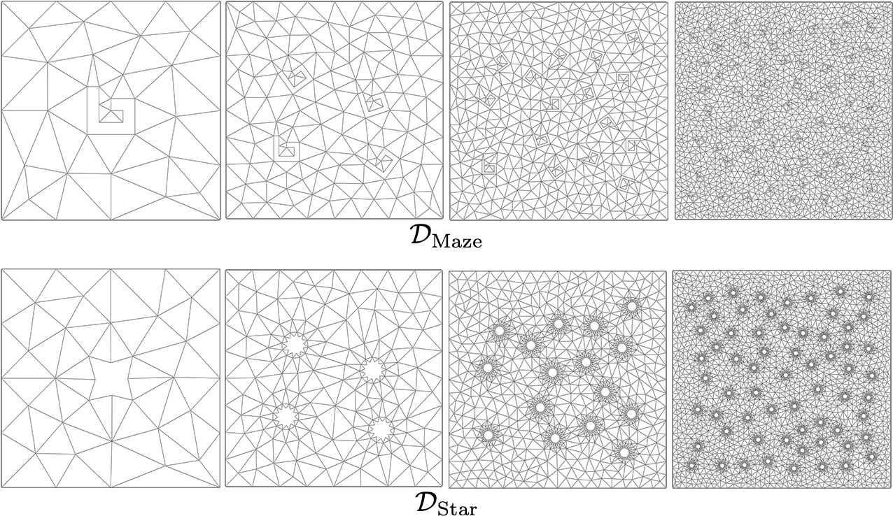
Figure 3: Meshes $\Omega_{0},\Omega_{2},\Omega_{4},\Omega_{6}$ from datasets $\mathcal{D}_{\rm{Maze}}$ and $\mathcal{D}_{\rm{Star}}$.

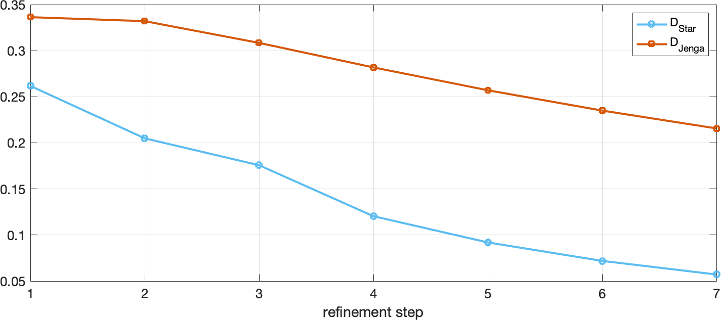
Figure 4: Evolution of the ratio $r_{E}/h_{E}$ for the meshes in datasets $\mathcal{D}_{\rm{Star}}$ and $\mathcal{D}_{\rm{Jenga}}$.

Mirroring datasets. As an alternative strategy to build a sequence of meshes whose elements are progressively smaller, we adopt an iterative mirroring technique: given a mesh $\mathcal{M}$ defined on $\Omega$, we generate a new mesh $\mathcal{M}^{\prime}$ containing four adjacent copies of $\mathcal{M}$, opportunely scaled to fit $\Omega$.
The starting point for the construction of a dataset is the first base mesh $\widehat{\Omega}_{0}$, which coincides with the first computational mesh $\Omega_{0}$. At every step $1\leq n\leq N$, a new base mesh $\widehat{\Omega}_{n}$ is built from the previous base mesh $\widehat{\Omega}_{n-1}$. The computational mesh $\Omega_{n}$ is then obtained by applying the mirroring technique $4^{n}$ times to the base mesh $\widehat{\Omega}_{n}$. This construction allows us to obtain a number of vertices and degrees of freedom in each mesh that is comparable to that of the meshes at the same refinement level in datasets $\mathcal{D}_{\rm{Maze}}$ and $\mathcal{D}_{\rm{Star}}$.

The $n$-th base mesh $\widehat{\Omega}_{n}$ of dataset $\mathcal{D}_{\rm{Jenga}}$ (Fig. 5, top) is built as follows. We start by subdividing the domain $(0,1)^{2}$ into three horizontal rectangles with area equal to $1/4$, $1/2$ and $1/4$ respectively. Then, we split the rectangle with area $1/2$ vertically, into two identical rectangles with area $1/4$. This concludes the construction of the base mesh $\widehat{\Omega}_{0}$, which coincides with mesh $\Omega_{0}$. At each next refinement step $n\geq 1$, we split the left-most rectangle in the middle of the base mesh $\widehat{\Omega}_{n-1}$ by adding a new vertical edge, and apply the mirroring technique to obtain $\Omega_{n}$. Despite being made entirely by simple rectangular elements, this mesh family is the most complex one: both $A_{n}$ and $e_{n}$ scale like $2^{n}$ and it breaks all the assumptions.

G2, G2-strong

because the ratio $|e|/h_{E}$ decreases unboundedly in the left rectangle $E$, as shown in Fig. 4. This implies that a lower bound with a uniform constant $\rho$ independent of $h$ cannot exist;

G1, G1-weak

since the length of the radius $r_{E}$ of the maximum disc inscribed into a rectangle is equal to $1/2$ of its shortest edge $e$, the ratio $r_{E}/h_{E}$ also decreases;

G3

because the number of edges of the top (or the bottom) rectangular element grows unboundedly;

G4

because the one-dimensional mesh built on the boundary of the top rectangular element cannot be subdivided into a finite number of quasi uniform sub-meshes. In fact, either we have infinite sub-meshes or an infinite edge ratio.

For the dataset $\mathcal{D}_{\rm{Slices}}$ (Fig. 5, middle), the $n$-th base mesh $\widehat{\Omega}_{n}$ is built as follows. First, we sample a set of points along the diagonal (the one connecting the vertices $(0,1)$ and $(1,0)$) of the reference square $[0,1]^{2}$, and connect them to the vertices $(0,0)$ and $(1,1)$. In particular, at each step $n\geq 0$, the base mesh $\widehat{\Omega}_{n}$ contains the vertices $(0,0)$ and $(1,1)$, plus the vertices with coordinates $(2^{-i},1-2^{-i})$ and $(1-2^{-i},2^{-i})$ for $i=1,\ldots,n+2$. Then, we apply the mirroring technique. Since no edge is ever split, we find that $e_{n}\sim c$, while $A_{n}\sim 2^{n}$. The dataset $\mathcal{D}_{\rm{Slices}}$ violates assumptions

G1, G1-weak

because, up to a multiplicative scaling factor depending on $h$, the radius $r_{E}$ is decreasing faster than the diameter $h_{E}$, which is constantly equal to $\sqrt{2}$ times the same scaling factor. Moreover, any finite subdivisions of the mesh elements would suffer the same issue;

G2-strong

the vertices sampled along the diagonal have accumulation points at $(0,1)$ and $(1,0)$, therefore the distance between two vertices decreases progressively.

In $\mathcal{D}_{\rm{Ulike}}$ (Fig. 5, bottom), we build the mesh $\widehat{\Omega}_{n}$ at each step $n\geq 0$ by inserting $2^{n}$ equispaced $U$-shaped continuous polylines inside the domain, creating as many $U$-like polygons. Then, we apply the mirroring technique as usual. Edge lengths scale exponentially and areas scale uniformly, i.e., $e_{n}\sim 2^{n}$, $A_{n}\sim c$, and the violated assumptions are:

G1, G1-weak, G2, G2-strong

for arguments similar to the ones seen for $\mathcal{D}_{\rm{Maze}}$;

G3

in order to preserve the connectivity, the lower edge of the more external $U$-shaped polygon in every base mesh must be split into smaller edges before applying the mirroring technique. Hence the number of edges of such elements cannot be bounded from above.

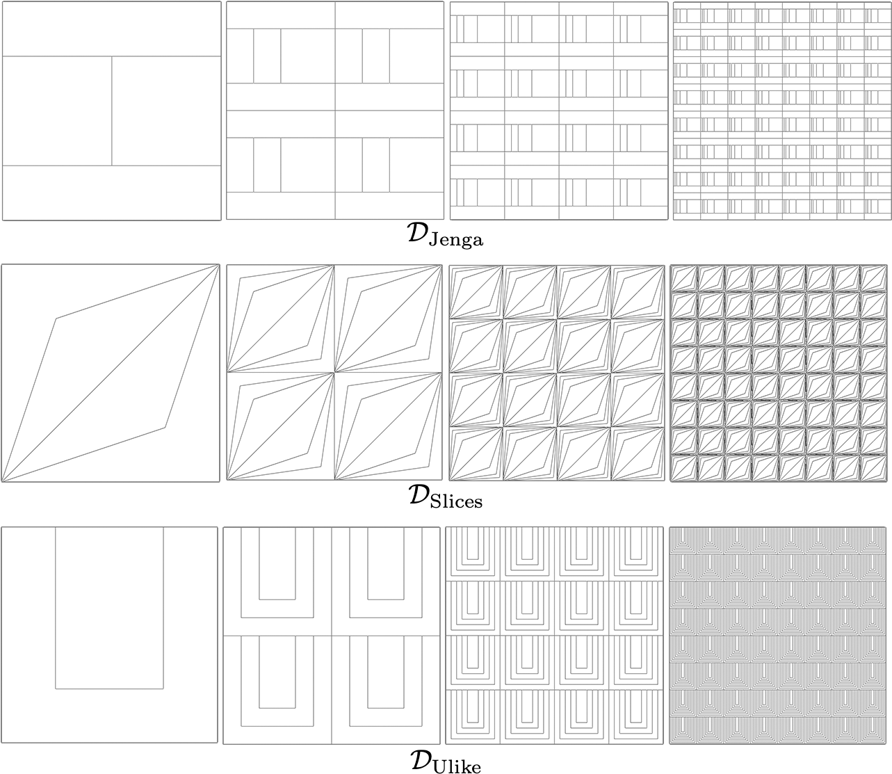
Figure 5: Meshes $\Omega_{0},\Omega_{1},\Omega_{2},\Omega_{3}$ from datasets $\mathcal{D}_{\rm{Jenga}}$, $\mathcal{D}_{\rm{Slices}}$ and $\mathcal{D}_{\rm{Ulike}}$.

Multiple mirroring datasets. As a final test, we modified datasets $\mathcal{D}_{\rm{Jenga}}$, $\mathcal{D}_{\rm{Slices}}$ and $\mathcal{D}_{\rm{Ulike}}$ in order to particularly stress the scaling indicators $A_{n}$ and $e_{n}$.
We obtained this by simply inserting four new elements at each step instead of one. The resulting datasets, $\mathcal{D}_{\rm{Jenga4}}$, $\mathcal{D}_{\rm{Slices4}}$ and $\mathcal{D}_{\rm{Ulike4}}$, are qualitatively similar to the correspondent mirroring datasets above. Each of these datasets respects the same assumptions of its original version, but the number of elements at each refinement step now increases four times faster. Consequently, the indicators $A_{n}$ and $e_{n}$ change from $2^{n}$ to $2^{4n}$, but $A_{n}$ remains constant for $\mathcal{D}_{\rm{Ulike4}}$, and $e_{n}$ remains constant for $\mathcal{D}_{\rm{Slices4}}$.

Table 1: Summary of the geometrical conditions violated and the asymptotic trend of the indicators $A_{n}$ and $e_{n}$ for all datasets. G1w and G2s stand for G1-weak and G2-strong, respectively, and $a$ is a constant such that $e<a<3$).

dataset	$\mathcal{D}_{\rm{Triangle}}$	$\mathcal{D}_{\rm{Maze}}$	$\mathcal{D}_{\rm{Star}}$	$\mathcal{D}_{\rm{Jenga}}$	$\mathcal{D}_{\rm{Slices}}$	$\mathcal{D}_{\rm{Ulike}}$
G1, G1w, G2s		$\times$	$\times$	$\times$	$\times$	$\times$
G2		$\times$		$\times$		$\times$
G3			$\times$	$\times$		$\times$
G4				$\times$
$A_{n}$	$c$	$a^{n}$	$n$	$2^{n}$	$2^{n}$	$c$
$e_{n}$	$c$	$n\log(n)$	$n$	$2^{n}$	$c$	$2^{n}$

4.2 VEM performance over the datasets

We solved the discrete Poisson problem (3) with the VEM (6) described in Section 2 for $k=1,2,3$ over each mesh of each of the datasets defined in Section 4.1, using as groundtruth the function

$$u(x,y)=\frac{\sin(\pi x)\sin(\pi y)}{2\pi^{2}},\hskip 8.5359pt(x,y)\in\Omega=(0,1)^{2}.$$ (56)

This function has homogeneous Dirichlet boundary conditions, and this choice was appositely made to prevent the boundary treatment from having an influence on the approximation error.

Performance indicators After computing the solution of the problem on a particular dataset, we want to measure the performance of the method over that dataset, that is, the accuracy and the convergence rate. We selected, among many possible alternatives, some quantities which can indicate if the error between the continuous solution $u$ and the computed solution $u_{h}$ is small and if the VEM worked properly in the computation of $u_{h}$. A more complete and accurate analysis of the possible performance indicators can be found in Section 5.2.

The approximation error might be measured in different norms: the most widely used in our framework are the relative $H^{1}$-seminorm and the relative $L^{2}$-norm (in the following we use the generic term norms to indicate both of them):

$$\frac{|u-u_{h}|_{1,\Omega}}{|u|_{1,\Omega}}\quad\text{and}\quad\frac{||u-u_{h}||_{0,\Omega}}{||u||_{0,\Omega}}.$$

In Fig. 6 and Fig. 7 we plot the two norms of the error generated by the VEM on each dataset as the number of DOFs increases (that is, as $n\to N$).

Another quantity, not directly related to the error, which can be of interest is the condition number of the matrices G and H (with the notation adopted in [6]):

$$\text{cond}(\textbf{G})=\|\textbf{G}\|\|\textbf{G}^{-1}\|,\qquad\text{cond}(\textbf{H})=\|\textbf{H}\|\|\textbf{H}^{-1}\|$$

Matrix G is involved in the computation of the local stiffness matrix and the projector $\Pi^{\nabla}_{k}$, while matrix H is involved in the computation of the local mass matrix and the projector $\Pi^{0}_{k}$.

Last, as an estimate of the error produced by projectors $\Pi^{\nabla}_{k}$ and $\Pi^{0}_{k}$, represented by matrices $\bm{\Pi}^{\nabla}_{k}$ and $\bm{\Pi}^{0}_{k}$, we check the identities

$$|\bm{\Pi}^{\nabla}_{k}\textbf{D}-\textbf{I}|=0\quad\text{and}\quad|\bm{\Pi}^{0}_{k}\textbf{D}-\textbf{I}|=0,$$ (57)

where for $k<3$ we have $\bm{\Pi}^{0}_{k}:=\bm{\Pi}^{\nabla}_{k}$. The computation of the projectors is obviously affected by the condition numbers of G and H, but the two indicators are not necessarily related.
Condition numbers and identity values for $k=1,2,3$ are reported in Table 2. All of these quantities are computed element-wise and the maximum value among all elements of the mesh is selected.

Performance The VEM performs perfectly over the reference dataset $\mathcal{D}_{\rm{Triangle}}$, and this guarantees for the correctness of the method. The approximation error evolves in accordance to the theoretical results (the slopes being indicated by the triangles) both in $L^{2}$ and in $H^{1}$ norms for all $k$ values, and condition numbers and optimal errors on the projectors $\Pi^{0}_{k}$ and $\Pi^{\nabla}_{k}$ remain optimal.

For the hybrid datasets $\mathcal{D}_{\rm{Star}}$ and $\mathcal{D}_{\rm{Maze}}$, errors decrease at the correct rate for most of the meshes, and only start deflecting for very complicated meshes with very high numbers of DOFs. These deflections are probably due to the extreme geometry of the star and maze polygons and not to numerical problems, as in both datasets we have cond(G) $<10^{6}$ and cond(H) $<10^{9}$, which are still reasonable values. Projectors seem to work properly: $|\bm{\Pi}^{\nabla}_{k}\textbf{D}-\textbf{I}|$ remains below $10^{-8}$ and $|\bm{\Pi}^{0}_{k}\textbf{D}-\textbf{I}|$ below $10^{-7}$. In a preliminary stage of this work, we obtained similar plots (not reported here) using other hybrid datasets built in the same way, with polygons surrounded by triangles. In particular, we did not notice big differences when constructing hybrid datasets as in Section 4.1 with any of the initial polygons of Section 5.3.

On the meshes from mirroring datasets $A_{n}$ or $e_{n}$ may scale exponentially instead of uniformly, as reported in Table 1. This reflects to cond(G) and cond(H), which grow up to, respectively, $10^{10}$ and $10^{14}$ for $\mathcal{D}_{\rm{Jenga}}$ in the case $k=3$. Nonetheless, the discrepancy of the projectors identities (57) remains below $10^{-5}$, which is not far from the results obtained with datasets $\mathcal{D}_{\rm{Maze}}$ and $\mathcal{D}_{\rm{Star}}$. The method exhibits an almost perfect convergence rate on dataset $\mathcal{D}_{\rm{Jenga}}$, even though $L^{2}$ and $H^{1}$ errors are bigger in magnitude than the ones measured for hybrid datasets. $\mathcal{D}_{\rm{Slices}}$ produces even bigger errors and a non-optimal convergence rate, and $\mathcal{D}_{\rm{Ulike}}$ is the dataset with the poorest performance, but the VEM still converges at a decent rate for $k>1$.
This may be due to the fact that for $k=1$ the DOFs correspond to the vertices of the mesh, which are disposed in a particular configuration that generates horizontal bands in the domain completely free of vertices, and therefore of data. For $k>1$ instead, we have DOFs also on the edges and inside the elements, hence the information is more uniformly distributed.

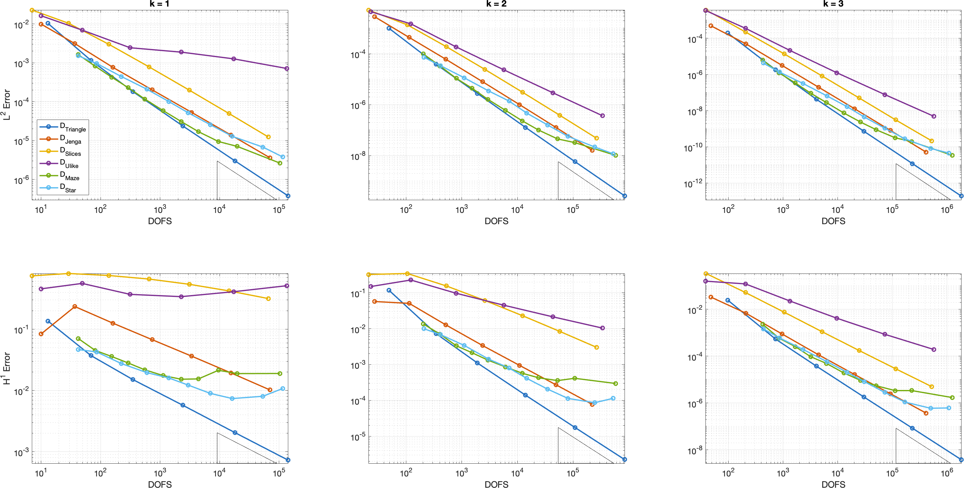
Figure 6: $L^{2}$-norm and $H^{1}$-seminorm of the approximation errors of the reference, hybrid and mirroring datasets for $k=1,2,3$.

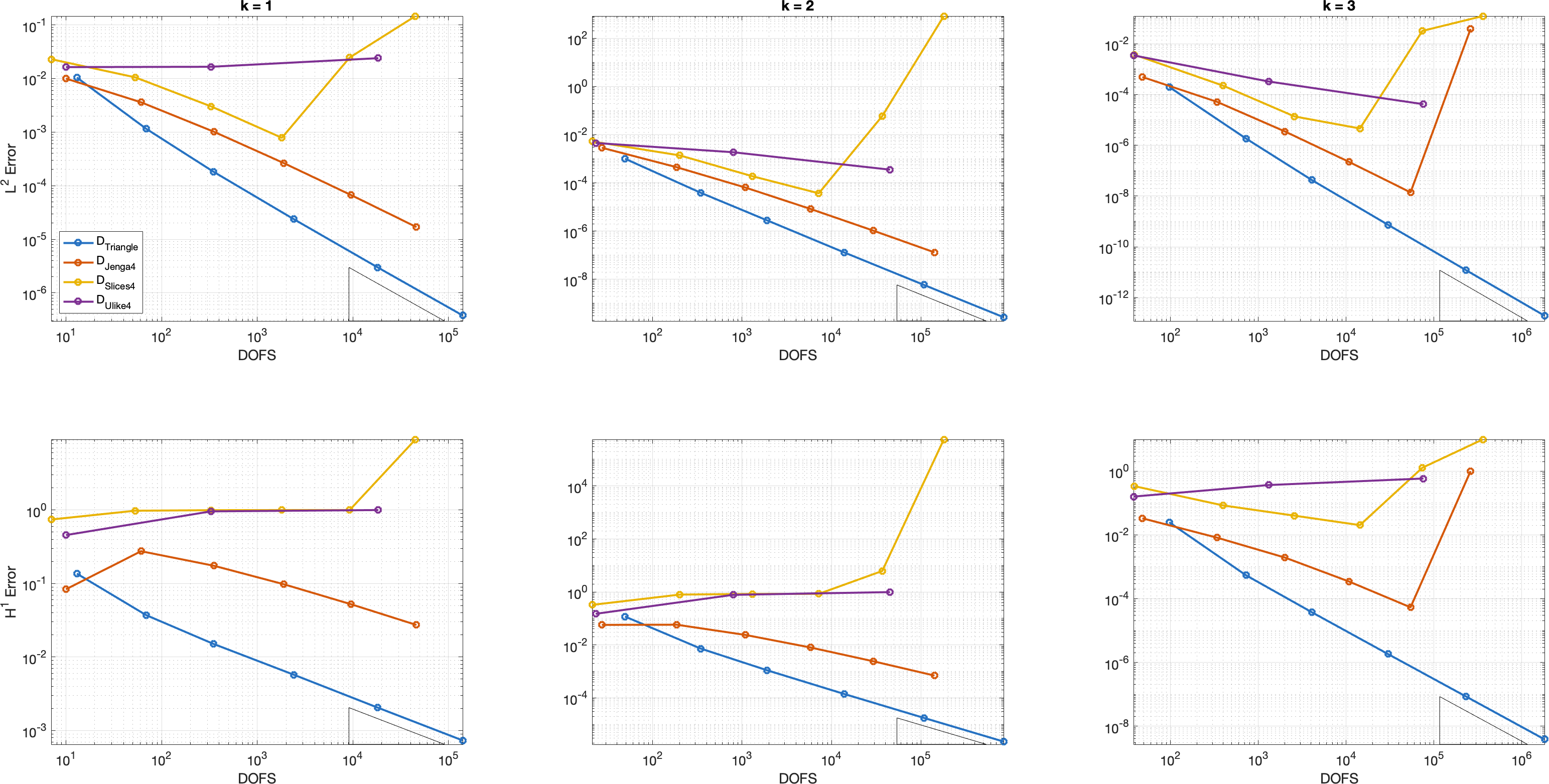
Figure 7: $L^{2}$-norm and $H^{1}$-seminorm of the approximation errors of the reference and multiple mirroring datasets for $k=1,2,3$.

In the case of multiple mirroring datasets the method diverges badly on all datasets (see Fig. 7), and this is principally due to the very poor condition numbers of the matrices involved in the calculations (see Table 2). The plots relative to datasets $\mathcal{D}_{\rm{Jenga4}}$ and $\mathcal{D}_{\rm{Slices4}}$ maintain a similar trend to those of $\mathcal{D}_{\rm{Jenga}}$ and $\mathcal{D}_{\rm{Slices}}$ in Fig. 6, until numerical problems cause cond(G) and cond(H) to explode up to over $10^{30}$ for $\mathcal{D}_{\rm{Jenga4}}$ and $10^{18}$ for $\mathcal{D}_{\rm{Slices4}}$. In such conditions, the projection matrices $\bm{\Pi}^{\nabla}_{k}$ and $\bm{\Pi}^{0}_{k}$ become meaningless and the method diverges. The situation slightly improves for $\mathcal{D}_{\rm{Ulike4}}$: cond(H) is still $10^{16}$, but the discrepancy of $\bm{\Pi}^{\nabla}_{k}$ and $\bm{\Pi}^{0}_{k}$ remain acceptable. As a result, the method on $\mathcal{D}_{\rm{Ulike4}}$ does not properly explode, but the approximation error and the convergence rate are much worse than those seen for $\mathcal{D}_{\rm{Ulike}}$ in Fig. 6.

Table 2: Summary of numerical performance for all datasets. We report the $\log_{10}$ of the original values for the condition number of G and H and the discrepancy of projection matrices $\bm{\Pi}^{\nabla}_{k}$ and $\bm{\Pi}^{0}_{k}$. Note that for $k<3$ we have $\bm{\Pi}^{0}_{k}:=\bm{\Pi}^{\nabla}_{k}$.

dataset	$\mathcal{D}_{\rm{Triangle}}$			$\mathcal{D}_{\rm{Maze}}$			$\mathcal{D}_{\rm{Star}}$			$\mathcal{D}_{\rm{Jenga}}$			$\mathcal{D}_{\rm{Slices}}$			$\mathcal{D}_{\rm{Ulike}}$			$\mathcal{D}_{\rm{Jenga4}}$			$\mathcal{D}_{\rm{Slices4}}$			$\mathcal{D}_{\rm{Ulike4}}$
$k$	1	2	3	1	2	3	1	2	3	1	2	3	1	2	3	1	2	3	1	2	3	1	2	3	1	2	3
cond(G)	0	2	5	2	3	6	1	3	6	1	5	10	2	4	6	1	4	7	6	18	31	6	8	10	2	6	11
cond(H)	2	5	7	2	5	8	3	6	9	4	9	14	2	8	10	3	7	10	13	26	39	2	15	18	5	10	16
$|\bm{\Pi}^{\nabla}_{k}\textbf{D}-\textbf{I}|$	-13	-11	-9	-12	-10	-8	-12	-10	-8	-12	-8	-5	-12	-10	-9	-13	-10	-8	-9	3	13	-8	-6	-5	-13	-8	-5
$|\bm{\Pi}^{0}_{k}\textbf{D}-\textbf{I}|$			-10			-8			-7			-5			-5			-7			20			8			-4

As a preliminary conclusion, by simply looking at the previous plots we observe that the relationship between the geometrical assumptions respected by a certain dataset and the performance of the VEM on it is not particularly strong. In fact, we obtained reasonable errors and convergence results on datasets violating several assumptions (all of them, in the case of $\mathcal{D}_{\rm{Jenga}}$).

5 Mesh quality metrics

The aim of this section is to introduce some geometrical parameters, that we will refer to as quality metrics, which are potentially well suited to measure the shape regularity of a polygon, and study, statistically, the behavior of a VEM solver, as such measures degrade. In the following we present a list of polygon quality metrics and different strategies to combine them to form a quality metric for a polygonal tessellation. We will also introduce a list of parameters providing us with different ways of measuring the performance of the VEM solver at hand.

5.1 Polygon quality metrics

Different parameters provide us with some information on how much an element is far from being “nice”, and the different assumptions presented in Section 3.1 give us a first list of possibilities. In the following we present the list of polygon quality metrics that we singled out for our study.

• Circumscribed circle radius (CC): this is defined as the radius of the smallest circle fully containing $P$. The parameter CC  is computed by treating the vertices of $P$ as a point cloud and running the Welzl’s algorithm to solve the minimum covering circle problem [62]. We point out that this choice does not yield the classical definition of circumscribed circle, requiring that all the vertices of the polygon lie on the circle, that does not necessarily exist for all polygons (Fig. 8).

  

  Figure 8: To be able to scale on general polygons, we define the radius of the circumscribed circle (CC) as the radius of the smallest circle containing the polygon itself. (Left) For a skinny triangle, CC is the radius of the smallest circle that passes through the endpoints of its longest edge (green), and not of the circle passing through all its three vertices (red). (Right) A general polygon and its CC.

• Inscribed circle radius (IC): this is defined as the radius of the biggest circle fully contained in $P$. For the computation of IC, starting from a Voronoi diagram of the edges of $P$, we select the corner in the diagram that is furthest from all edges as center of the circle. The radius of the IC is the minimum distance between such point and any of the edges of $P$. For the computation of the diagram of the set of edges, which, differently from the point case, has curved boundaries between cells, we apply the Boost Polygon Library [58].

• Circle ratio (CR): the ratio between IC  and CC. Differently from the previous two, this measure does not depend on the scale of the polygon, and is always defined in the range $(0,1]$.

• Area (AR): the area of the polygon $P$.

• Kernel area (KE): the area of the kernel of the polygon, defined as the set of points $p\in P$ from which the whole polygon is visible. If the polygon is convex, then the area of the polygon and the area of the kernel are equal. If the polygon is star-shaped, then the area of the kernel is a positive number. If the kernel is not star-shaped, then the kernel of the polygon is empty and KE will be zero.

• Kernel-area/area ratio (KAR): the ratio between the area of the kernel of $P$ and its whole area. For convex polygons, this ratio is always 1. For concave star-shaped polygons, KAR  is strictly defined in between 0 and 1. For non star-shaped polygons, KAR  is always zero.

• Area/perimeter ratio (APR), or compactness: defined as $\frac{2\pi*\textsf{area}(P)}{\textsf{perimeter}(P)^{2}}$. This measure reaches its maximum for the most compact 2D shape (the circle), and becomes smaller for less compact polygons.

• Shortest edge (SE): the length of the shortest edge of $P$.

• Edge ratio (ER): the ratio between the length of the shortest and the longest edge of $P$.

• Minimum vertex to vertex distance (MPD), which is the minimum distance between any two vertexes in $P$. MPD is always less then or equal to SE. In case the two vertexes realizing the minimum distance are also extrema of a common edge, MPD  and SE  are equals.

• Minimum angle (MA): the minimum inner angle of the polygon $P$.

• Maximum angle (MXA): the maximum inner angle of the polygon $P$.

• Number of edges ($N^{\mathcal{S}}$): the number of edges of the polygon.

• Shape regularity (SR): the ratio between the radius of the circle inscribed in the kernel of the element and the radius CC of the circumscribed circle (Fig. 9). This assumes the value $0$ for polygons which are not star shaped.

  Figure 9: Polygon shape regularity expressed in terms of the ratio between the radius maximal ball inscribed in the kernel of the polygon ($d$), and the radius of the maximal ball inscribing the element ($D$).

Remark that, while in triangular elements all the previous metrics are strictly bound to each other, for general polygons this is not the case, and, given a couple of such metrics, it is in general possible to find sequences of polygons for which one of the two degenerates, while the other stays constant. Remark also that some of the metrics, namely CR, KAR, APR, ER, MA, MXA, $N^{\mathcal{S}}$ and SR, are scale invariant, and only depend on the shape of the polygon and not on its size.

Aggregating polygon quality metrics into mesh quality metrics Let now consider a tessellation $\Omega_{h}=\{P_{i},i=1,\cdots,N\}$ with $N$ elements. For ${\mathfrak{m}}$ being any of the above polygon quality metrics we can consider the vector

$$\bm{{\mathfrak{m}}}(\Omega_{h})=({\mathfrak{m}}(P_{1}),\cdots,{\mathfrak{m}}{(P_{N})}).$$

Starting from such a vector we can define a measure of the quality of the whole mesh, by following different strategies. More precisely, we considered the following possibilities.

• Average

  $${\mathfrak{m}}_{\text{av}}(\Omega_{h})=\text{average}(\bm{{\mathfrak{m}}}(\Omega_{h}))=\frac{1}{N}\sum_{i=1}^{N}{\mathfrak{m}}(P_{i}).$$

• Euclidean norm

  $${\mathfrak{m}}_{\text{l}_{2}}(\Omega_{h})=\|\bm{{\mathfrak{m}}}(\Omega_{h})\|_{2}=\left(\sum_{i=1}^{N}{\mathfrak{m}}(P_{i})^{2}\right)^{1/2}$$

• Maximum

  $${\mathfrak{m}}_{\text{max}}(\Omega_{h})=\max\{{\mathfrak{m}}(P_{i}),i=1,\cdot,N\}$$

• Minimum

  $${\mathfrak{m}}_{\text{min}}(\Omega_{h})=\min\{{\mathfrak{m}}(P_{i}),i=1,\cdot,N\}$$

To these four strategies, we add a fifth strategy, namely we define ${\mathfrak{m}}_{\text{worst}}$ as the one, between ${\mathfrak{m}}_{\text{min}}$ and ${\mathfrak{m}}_{\text{max}}$, that singles out the worst polygon. More precisely, for ${\mathfrak{m}}\in\{IC,CR,KE,KAR,APR,SE,ER,MPD,MA,SR\}$ we set

$${\mathfrak{m}}_{\text{worst}}(\Omega_{h})={\mathfrak{m}}_{\text{min}}(\Omega_{h}),$$

while for ${\mathfrak{m}}\in\{CC,MXA,N^{\mathcal{S}}\}$ we set

$${\mathfrak{m}}_{\text{worst}}(\Omega_{h})={\mathfrak{m}}_{\text{max}}(\Omega_{h}).$$

5.2 Performance indicators

Let us now consider how we can measure the performance of a PDE solver. Depending on the context, saying that a solver is “good” can have different meanings. Typically, the first thing that comes to mind, is that a solver is good when the error between the computed and the true solution is small. However the error might be measured in different norms: for instance, while the most natural norm in our framework is the $H^{1}$ norm (which is spectrally equivalent to the energy norm), if one is interested in the point value of the solution, the right information on the accuracy of the method is provided by the $L^{\infty}$ norm of the error. The $L^{2}$ norm of the error is also frequently used to measure the accuracy. On the other hand, other quantities, not directly related to the error, can be of interest. For instance, if the problem considered involves inexact data, in order to limit the effect on the computed solution of the error on the data, the condition number of the stiffness matrix in the linear system of equations stemming from the discrete problem (6) should be kept as small as possible, compatibly with the known fact that such a quantity increases as the mesh size decreases. The condition number of the stiffness matrix is also of interested if one aims at solving a large number of different problems, therefore needing a good computational performance of the numerical method. Here we introduce the different performance indicators that we chose to consider in our statistical analysis of the the Virtual Element Method.

Energy norm error. The first indicator that we consider is the error between the computed solution $u_{h}$ and the continuous solution $u$, measured in the energy norm. We recall that the quantity on the left hand side of inequality (24) is not computable. What is then usually done is to evaluate instead some computable quantity, such as the energy norm relative to the discrete equation, or the broken $H^{1}(\Omega_{h})$ norm of $u-\Pi^{\nabla}u_{h}$. For our statistical analysis we chose, as first performance indicator

$$\mathbf{p}_{1}=\frac{\sqrt{a_{h}(u_{h}-u_{I},u_{h}-u_{I})}}{\sqrt{a_{h}(u_{I},u_{I})}}.$$

Observe that this indicator depends on the data $f$ and $g$ of the model problem considered, so that for different values of such data we have different values of the indicator.

$L^{\infty}$ error. In the finite element framework, under a shape regularity condition for the underlying triangular/quadrangular mesh, it is possible to bound, a priori, the maximum pointwise error. More precisely, under suitable assumptions on the discretization space which are satisfied by the most commonly used finite elements, if $u_{h}$ is the finite element solution to Problem (1)–(2) defined on a quasi uniform triangular/quadrangular grid of mesh size $h$, it is possible to prove (see [55]) that

$$\|u-u_{h}\|_{0,\infty,\Omega}\leq Ch_{\text{max}}^{k}\|u\|_{k,\infty,\Omega}.$$

While to our knowledge the problem of giving an $L^{\infty}$ a priori bound on the error for the virtual element method has not yet been addressed in the literature, measuring the error in such a norm is relevant to many applications. It is then interesting to measure such an error and see how it is affected by the shape of the elements of the tessellation. However, also in this case, as we do not have access to the point values of the discrete function $u_{h}$, we will instead compute, as a performance indicator, the quantity

$$\mathbf{p}_{2}=\frac{\max_{i}|\mathrm{dof}_{i}(u_{h}-u)|}{\max_{i}|\mathrm{dof}_{i}(u)}.$$

Also this indicator depends on the data $f$ and $g$ of the model problem considered.

$L^{2}$ error. The third quantity that we consider, is the $L^{2}$ norm of the error. As usual, the proof of an inequality of the form (25) involves a duality argument and relies on the same a priori interpolation estimates used for proving (24). It requires, therefore, the same shape regularity assumption on the tessellation. As for the $H^{1}$ and the $L^{\infty}$ norm errors, the $L^{2}$ norm of the error is not computable, and we replace it, in our experiments with the quantity

$$\mathbf{p}_{3}=\frac{\|u_{h}-\Pi^{0}_{k}u\|_{0,\Omega}}{\|\Pi^{0}_{k}u\|_{0,\Omega}},$$

Also this indicator depends on the data $f$ and $g$ of the model problem considered.

Condition number. The condition number of the global stiffness matrix has a twofold effect:

• it provides reliable information on the efficiency of iterative solvers for the linear system arising from the discretization, ad on the need (or lack thereof) of resorting to some kind of preconditioning;

• more importantly, it provides a bound on how errors are propagated and, possibly, amplified, in the solution process. We recall, in fact, that the condition number is defined as

  $$\kappa(\mathbf{R})=\|\mathbf{R}\|\,\|\mathbf{R}^{-1}\|,$$

  where $\mathbf{R}$ is the stiffness matrix stemming from equation (6). A large condition number for $\mathbf{R}$ might signify that the norm of $\mathbf{R}^{-1}$ is large. In turn, this implies that possible errors on the evaluation of right hand side of (6), which might derive not only from round off, but also from error on the data, are amplified by the solver resulting in a possibly much larger error in the computed discrete solution.

Estimating, a priori, the condition number of the stiffness matrix $\mathbf{R}$ is not difficult and relies on the use of an inverse inequality of the form

$$\|v_{h}\|_{1,\Omega}\leq C_{\text{inv}}h_{\text{min}}^{-1}\|v_{h}\|_{0,\Omega}.$$ (58)

Under assumptions G1 and G2, such an inequality can be proven to hold with a constant $C_{\text{inv}}$ independent of the polygon. If (58) holds, and if the chosen scaling for degrees of freedom is such that, letting $v_{h}\in V_{h}$ and $\mathbf{v}$ the vector of its degrees of freedom, we have

$$\|v_{h}\|_{0,\Omega}^{2}\simeq\mathbf{v}^{T}\mathbf{v}$$ (59)

(if assumptions G1 and G2 hold, this is always possible [36, 23]), then, for $\lambda$ eigenvalue of $\mathbf{R}$ and $\mathbf{v}$ correponding eigenvector, with $v_{h}$ denoting the corresponding function in $V_{h}$, we can write

$$\mathbf{v}^{T}\mathbf{v}\lesssim\|v_{h}\|^{2}_{0,\Omega}\leq\|v_{h}\|_{1,\Omega}^{2}\lesssim a_{h}(v_{h},v_{h})=\mathbf{v}^{T}\mathbf{R}\mathbf{v}=\lambda\mathbf{v}^{T}\mathbf{v},$$

as well as

$$\lambda\mathbf{v}^{T}\mathbf{v}=\mathbf{v}^{T}\mathbf{R}\mathbf{v}=a_{h}(v_{h},v_{h})\lesssim\|v_{h}\|_{1,\Omega}^{2}\leq C_{\text{inv}}h_{\text{min}}^{-2}\|v_{h}\|_{0,\Omega}\lesssim C_{\text{inv}}h^{-2}\mathbf{v}^{T}\mathbf{v}$$

finally yielding

$$\mathbf{v}^{T}\mathbf{v}\lesssim\lambda\mathbf{v}^{T}\mathbf{v}\lesssim C_{\text{inv}}h_{\text{min}}^{-2}\mathbf{v}^{T}\mathbf{v},$$

which implies

$$\kappa_{2}(\mathbf{R})\lesssim C_{\text{inv}}h_{\text{min}}^{-2}.$$

While the geometry of the elements also affects the implicit constant in the above inequality in different way (in particular through the continuity and coercivity constants and through the constants implicit in the equivalence relation (59)), we underlined here the effect of the constant appearing in the inverse inequality (58). Observe that if Assumption G2 is violated, then $C_{\text{inv}}$ is known to explode as the ratio between the diameter and the length of the smaller edge.

As computing the condition number exactly can be, for large matrices, extremely expensive, we used, as the performance indicator $\mathbf{p}_{4}$, a lower estimate of the $1$-norm condition number, computed by the Lanczos method, according to [42, 43].

Condition number after preconditioning. As already observed, for ill conditioned stiffness matrices, it is customary to resort to some form of preconditioning, and, consequently, a fairer estimation of the efficiency attained by a given solver requires taking into account the effect of preconditioning. Several approaches are available to precondition the stiffness matrix arising from the VEM discretization. We recall, among others, preconditioners based on domain decomposition, such as Schwarz [30], and FETI-DP and BDDC [22, 23], and multigrid [4]. Here we rather consider a simpler algebraic preconditioner, namely, the Incomplete Choleski factorization preconditioner [41]. Also here we use, as the preformance indicator $\mathbf{p}_{5}$, the lower estimate of the $1$-norm condition number of the preconditioned stiffenss marix, computed according to [42, 43].

Constant in the error estimate. While the theoretical error bound (24) puts forward the dependence of the error, measured in the $H^{1}(\Omega)$ norm, on the diameter of the largest element in the tessellation, the correlation analysis which, we will present in Section 5.3, shows a higher correlation of the error with the average diameter size, suggesting that, in practice, an estimate such as

$$\|u-u_{h}\|_{1,\Omega}\leq C(u)h_{\text{av}}^{k}$$ (60)

might hold. Of course, for fixed tessellation $\Omega_{h}$ and solution $u$ an equality will hold in (60), for a suitable constant $C(u)$ depending on the tessellation $\Omega_{h}$. We then use such a constant as a performance indicator $\mathbf{p}_{6}$:

$$\mathbf{p}_{6}=\frac{\mathbf{p}_{1}}{h_{\text{av}}^{k}}.$$

Aubin-Nitsche trick constant. In the finite element framework, the Aubin-Nitsche duality trick allows to bound the $L^{2}$-norm of the error as

$$\|u-u_{h}\|_{0,\Omega}\leq C_{\text{AN}}h_{\text{max}}\|u-u_{h}\|_{1,\Omega},$$

from which a bound of the form (25) immediately results. While an analogous estimate cannot be proven for the VEM method, for which (25) is proven directly, as, once again, the two quantities $\|u-u_{h}\|_{0,\Omega}$ and $h_{\text{max}}\|u-u_{h}\|_{1,\Omega}$ are both positive and finite, the above inequality can be replaced by an equality for a given constant $C_{\text{AN}}$, depending on the data and on the tessellation. Also in this case our correlation suggests to replace, in an estimate of this kind, the diameter $h_{\text{max}}$ of the largest element with the average diameter, and we propose, as a performance indicator, the quantity

$$\mathbf{p}_{7}=\frac{\mathbf{p}_{2}}{h_{\text{av}}\mathbf{p}_{1}}.$$

Effectiveness of the preconditioner. The last performance indicator aims at evaluating if and how the geometry of the tessellation affects the effectiveness of the preconditioner by comparing the condition number of the preconditioned stiffness matrix with the one of the same matrix without any preconditioning. More precisely, the last performance indicator is defined as

$$\mathbf{p}_{8}=\frac{\mathbf{p}_{5}}{\mathbf{p}_{4}}.$$

Remark that we expect $\mathbf{p}_{8}$ to be less than $1$. $\mathbf{p}_{8}$ close to $1$ indicates an ineffective preconditioner, while $\mathbf{p}_{8}\ll 1$ indicates that the preconditioner is performing its role, while $\mathbf{p}_{8}\geq 1$ indicates the failure of the preconditioning algorithm.

5.3 Results

We considered two different test problem corresponding to two different solutions to the Poisson equation (1)–(2), both with $\Omega=(0,1)^{2}$.

Test 1

For the first test problem, the groundtruth is, once again,

$$u_{1}(x,y)=\frac{\sin(\pi x)\sin(\pi y)}{2\pi^{2}}.$$

Test 2

For the second test problem the groundtruth is the Franke function, namely

$$u_{2}(x,y):=\frac{3}{4}e^{-\left((9x-2)^{2}+(9y-2)^{2}\right)/4}+\frac{3}{4}e^{-\left((9x+1)^{2}/49+(9y+1)/10\right)}\\ +\frac{1}{2}e^{-\left((9x-7)^{2}+(9y-3)^{2}\right)/4}+\frac{1}{5}e^{-\left((9x-4)^{2}+(9y-7)^{2}\right)}.$$

We solved each problem with the VEM solver of order $k=1,2,3$ on 260 hybrid tessellations explicitly designed to progressively stress the polygon quality metrics described in Sect. 5.1. Specifically, a family of parametric polygons have been designed: the baseline configuration of each polygon (P(0)) does not present critical geometric features, and 20 versions of the same polygon are generated by progressively deforming the baseline by a parameter t. Each polygon (its baseline version and its deformations) is placed at the center of a canvas representing the squared domain $[0,1]^{2}$. the space of the domain complementary to the polygon is filled with triangles [56] [45]. Figure 10 shows the list of our parametric polygons and how they have been used to generate the dataset. Note that the parametric polygons ”maze” and ”star” are similar to the initial polygons of the hybrid datasets defined in Section 4.1, meaning that they contain the same pathologies even if edges and areas scale differently. The resulting meshes, however, have little in common, as meshes from $\mathcal{D}_{\rm{Maze}}$ and $\mathcal{D}_{\rm{Star}}$ contain several of such polygons with different sizes.

Figure 10: A subset of meshes in our dataset. On the left column, the list of names associated to parametric polygons (in red). On the top row, the values of the deformation parameter.

For each test case we compute the 5 performance indexes $\mathbf{p}_{1}$, $\mathbf{p}_{2}$, $\mathbf{p}_{3}$, $\mathbf{p}_{6}$, $\mathbf{p}_{7}$ corresponding to each tessellation. Moreover, for each tessellation, we computed the three performance indexes $\mathbf{p}_{4}$, $\mathbf{p}_{5}$ and $\mathbf{p}_{8}$, for a grand total of 13 performance indexes for each tessellation. We then computed the Spearman correlation index [60, 50] between the 14 quality metrics, with the five aggregation methods, and the 13 performance indexes. The results are displayed in figure 11. As the Euclidean norm aggregation method gives results that are substantially similar to the average aggregation method and as the worst aggregation method summarized the most significant of the minimum and maximum aggregation methods, we only show the results for average and worst aggregation method.

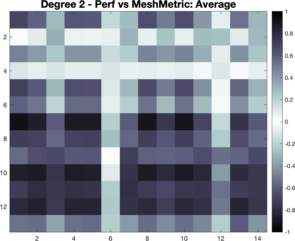
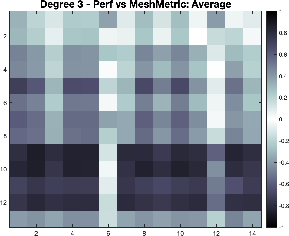
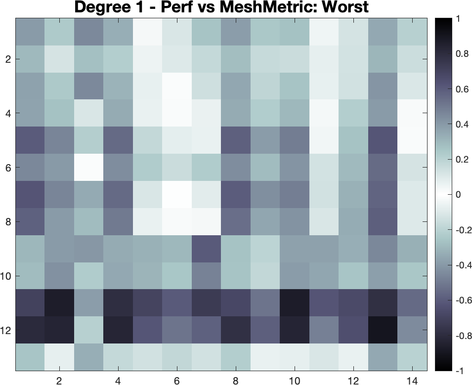
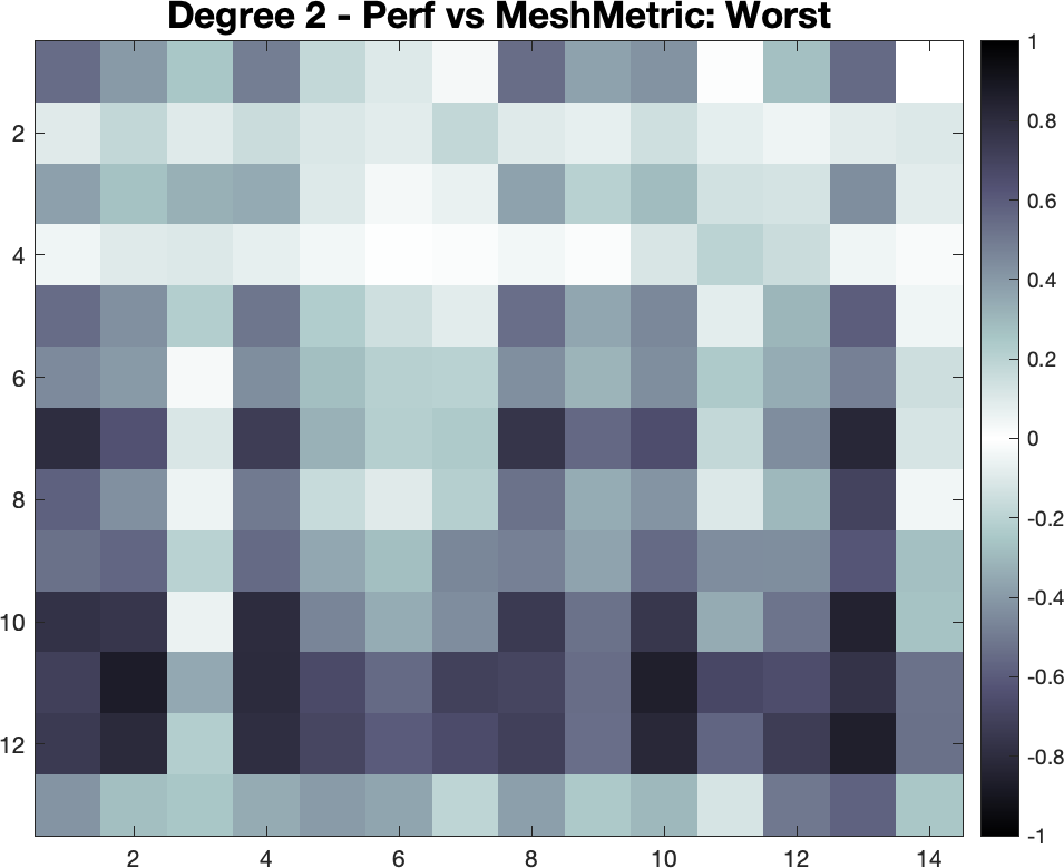
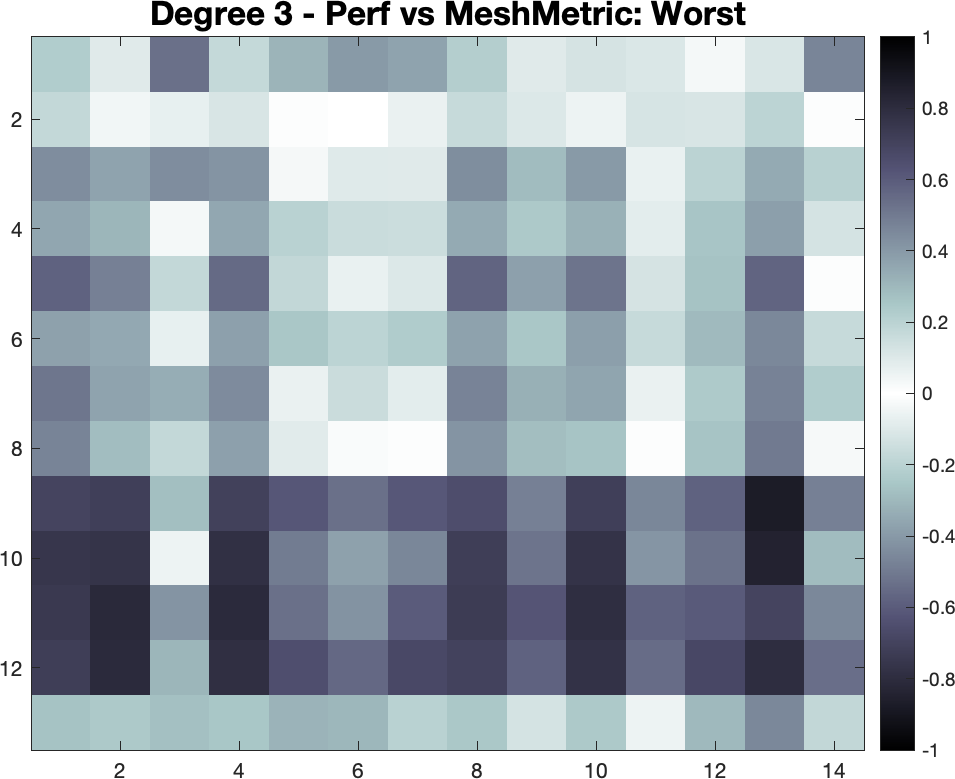
Figure 11: Mesh metrics (average agglomeration method, top and worst agglomeration method, bottom) vs Performance metrics for $k$ equals $1$ through $3$.

We next consider the cases that result in the overall lowest and highest correlation index. For such cases, we present the related scatterplots (displayed either in semi-logarithmic or in logarithmic scale). More precisely the scatterplot corresponding to low correlation are shown in Figure 12, while in Figure 13 we can look at the scatterplots corresponding to the high correlation cases. The first thing that jumps to the eye is that all high correlation case except one correspond to the average aggregation method, while the converse holds for the low correlation (all cases but two correspond to the worst aggregation method). Looking at Figure 12 we also see that the SR metric has low correlation with the error in the energy norm. This confirms the experimental observations, already pointed out in the literature, and is particularly interesting, as it shows that violating Assumption G1, which is the commonly used assumption in the analysis of VEM methods, does not necessarily result in a deterioration of the accuracy of the method. This suggests to try to carry out the convergence analysis in the absence of such a bound (and, in particular, for meshes of non star shaped polygons). The minimum and maximum angle also seem to have little correlation with the error. Conversely, two quantities that are clearly highly correlated with several of the metrics are the constants in the error estimate $\mathbf{p}_{6}^{(1)}$ and $\mathbf{p}_{6}^{(2)}$ and the Aubin Nitsche trick constants $\mathbf{p}_{7}^{(1)}$ and $\mathbf{p}_{7}^{(2)}$. We also observe that the constant in the error bound is highly correlated with the highest number of edges. This is also very interesting, as it suggests that even a single polygon with a high number of edges can affect the performance of the method. It is then worth devoting some effort to the design of variants of the VEM, aimed at attaining robustness with respect to the number of edges.

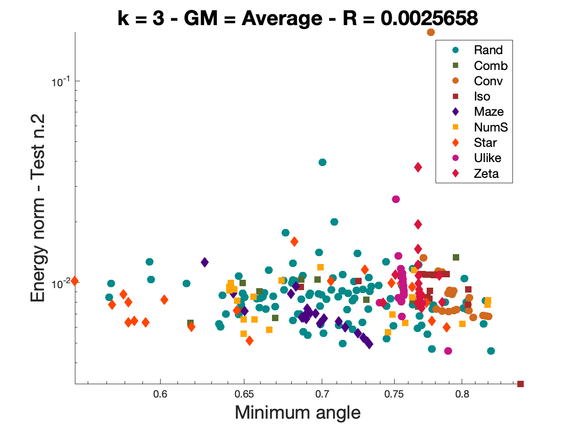
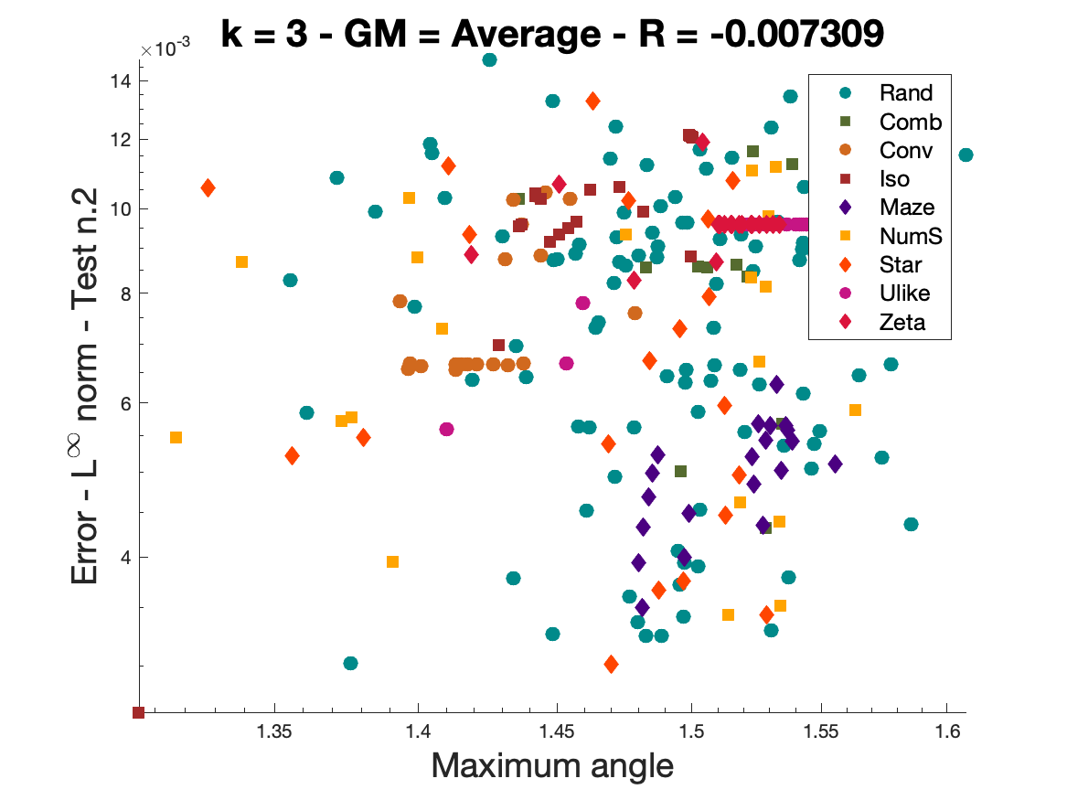
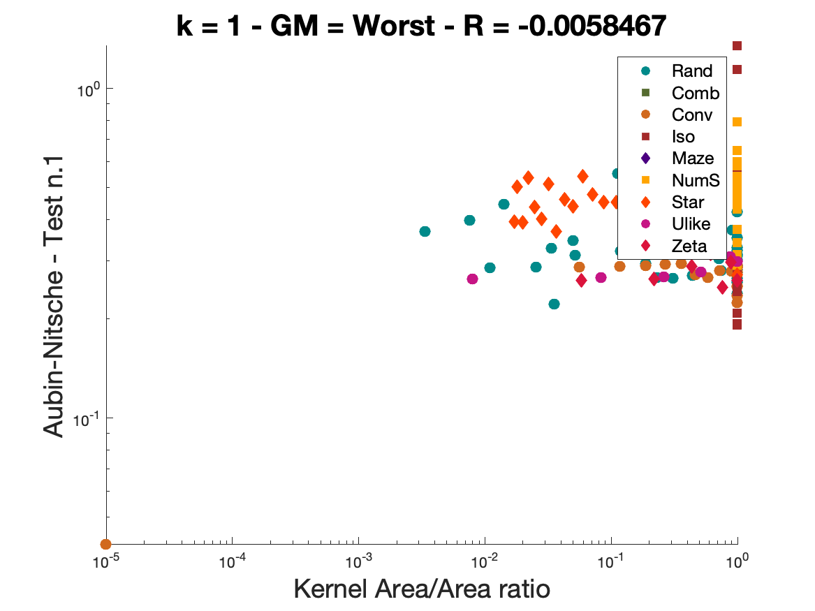
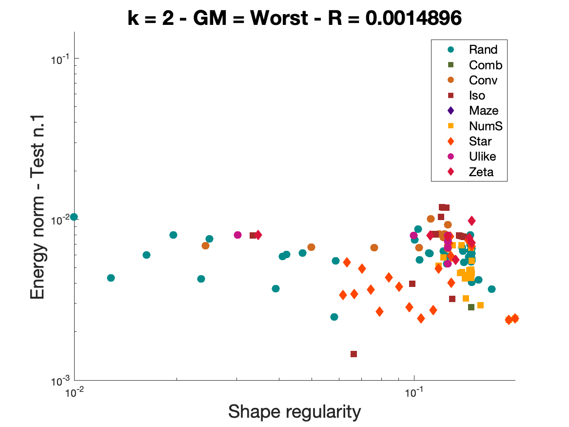
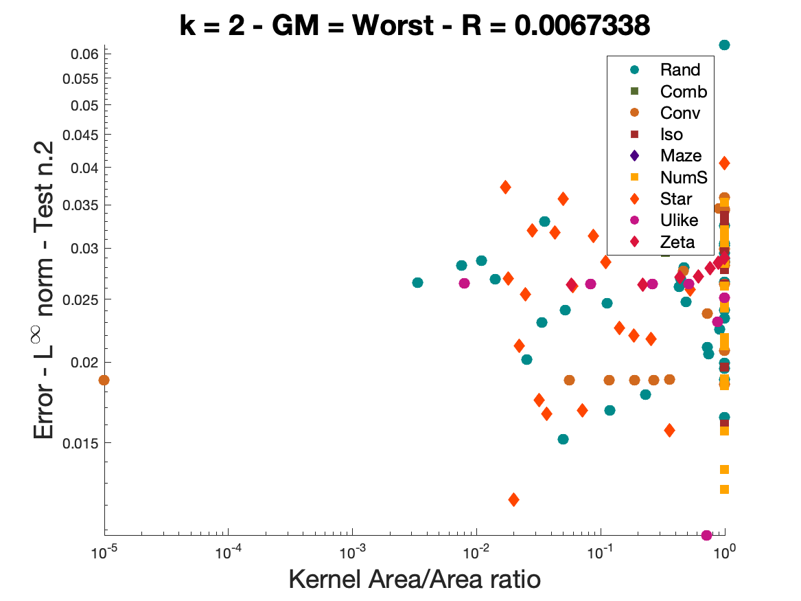
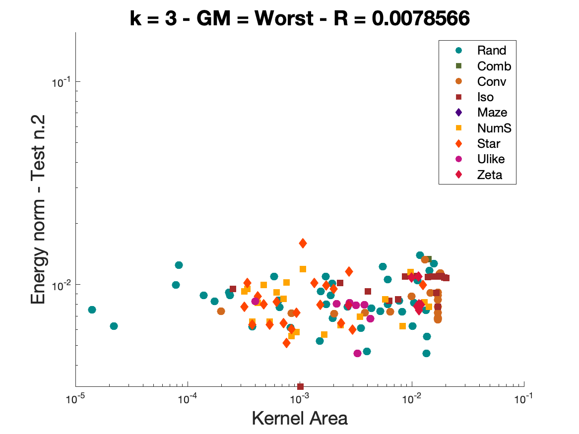
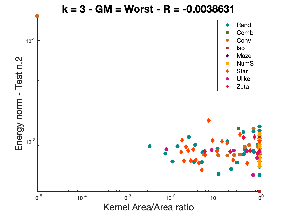
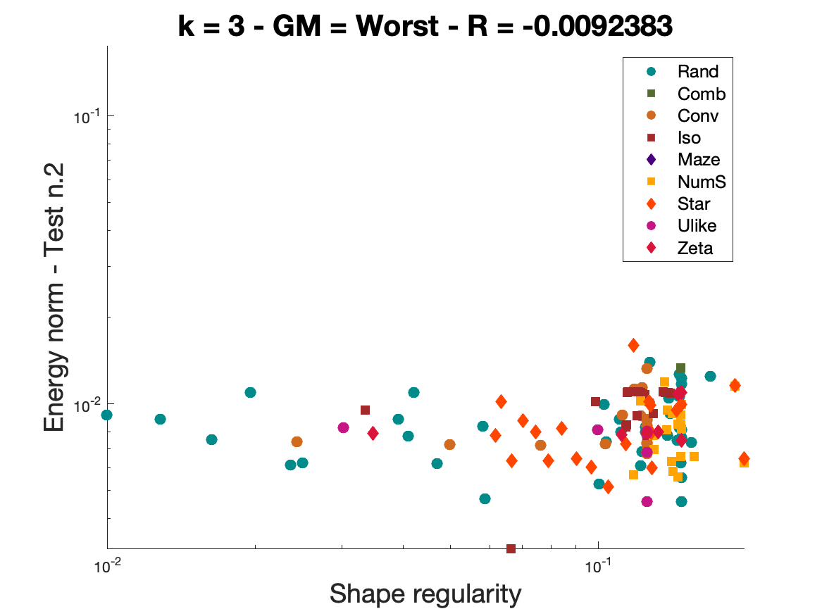
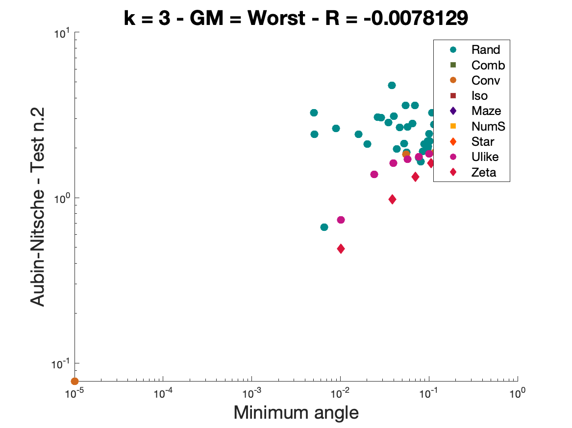
Figure 12: Scatterplots corresponding to an absolute value of the Spearman correlation lower than .03. On the x-axis the geometric metric, on the $y$-axis the performance metric.

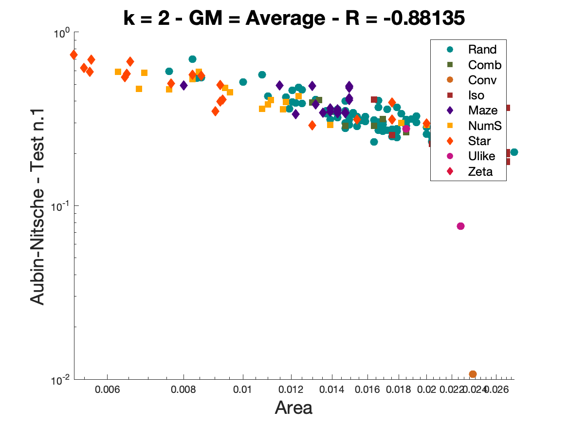
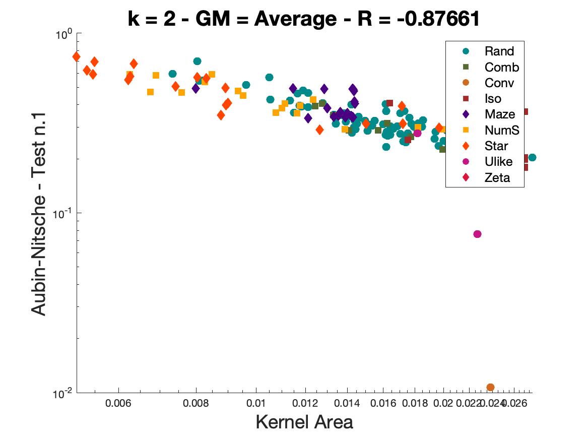
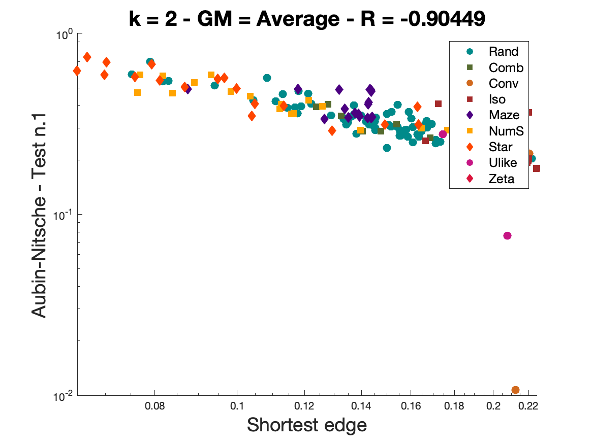
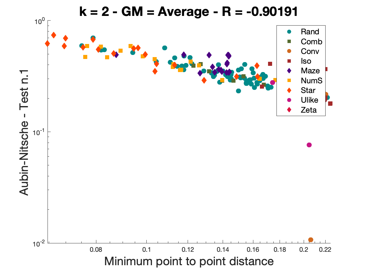
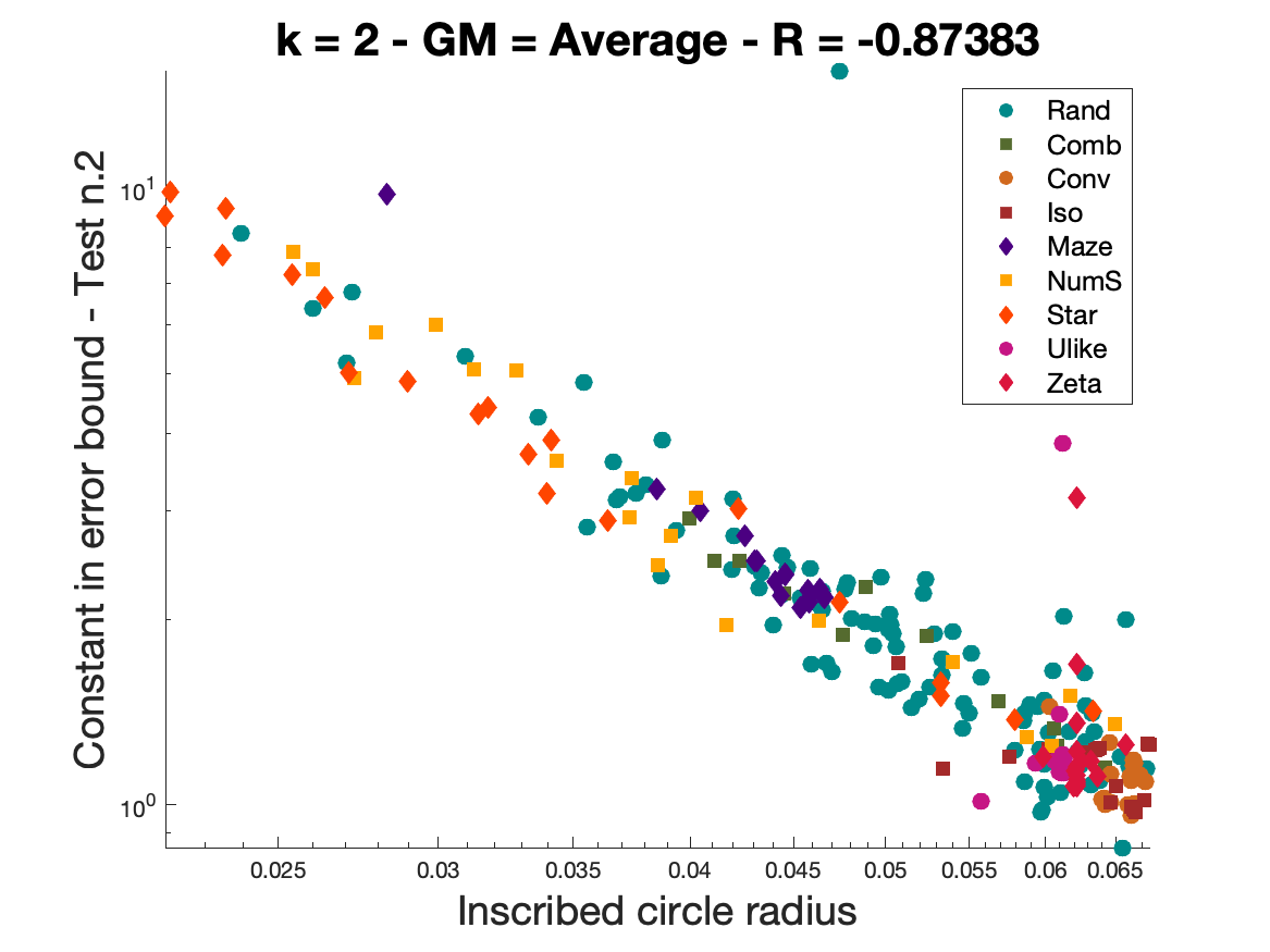
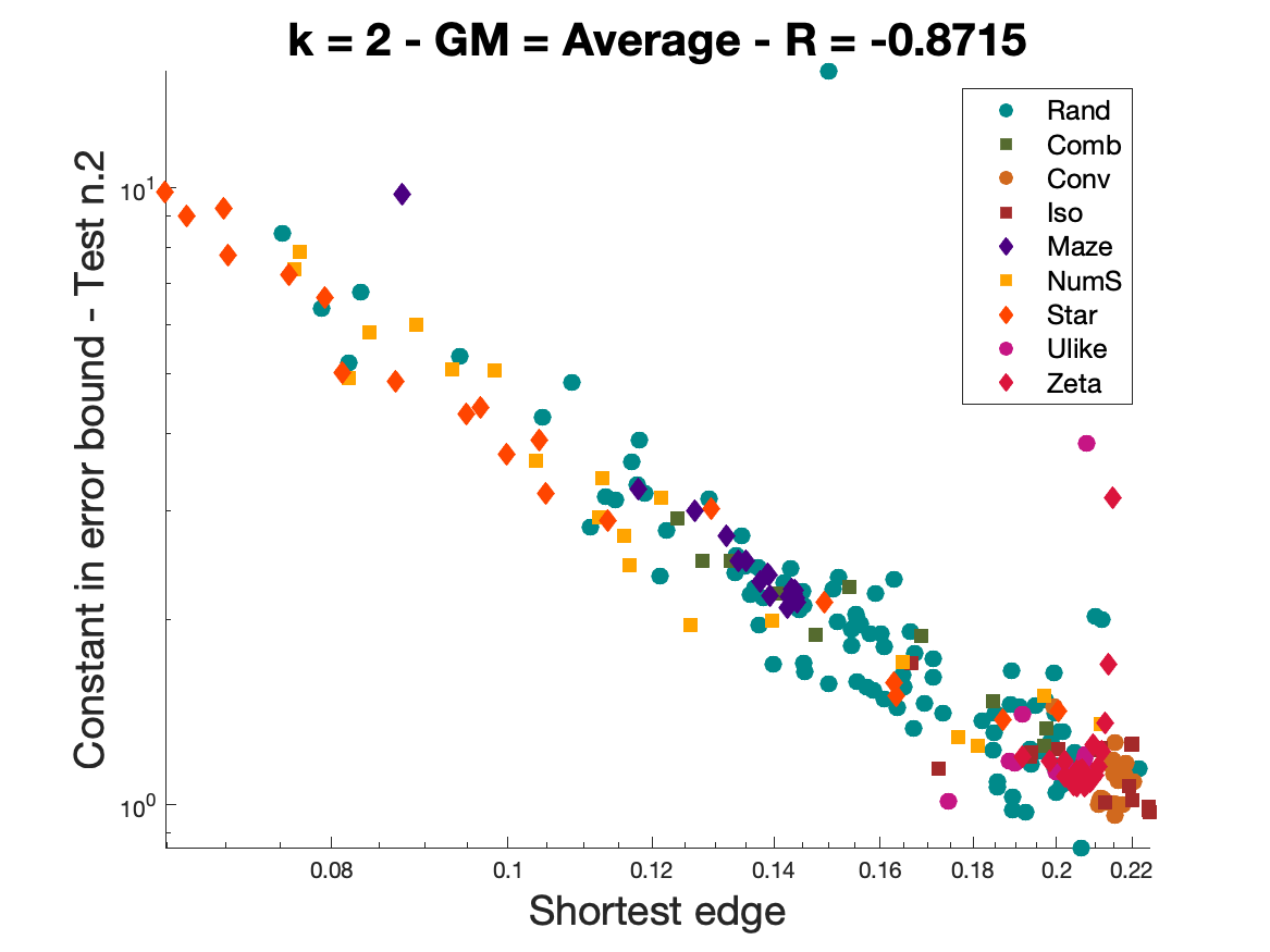
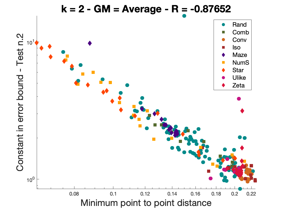
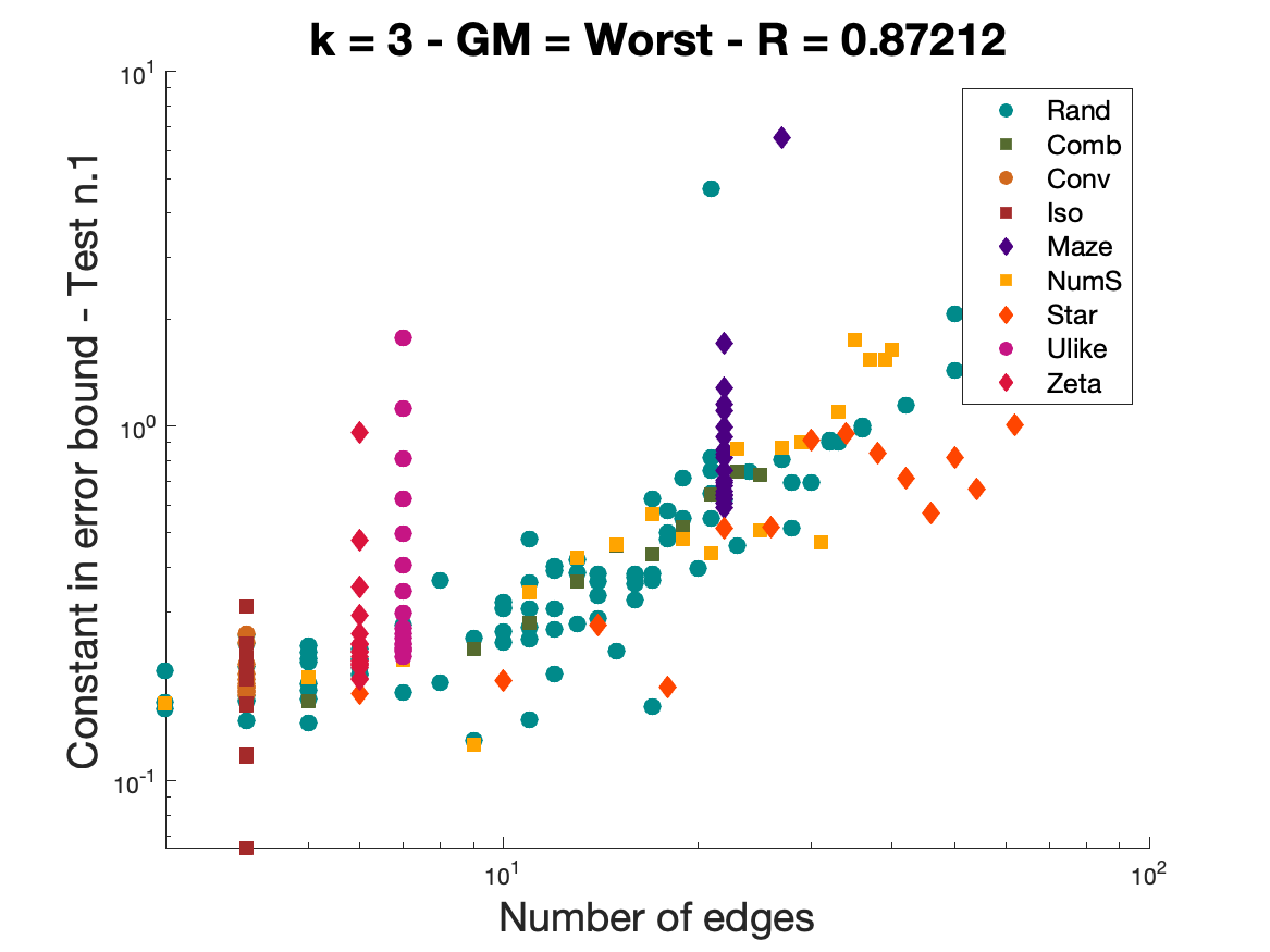
Figure 13: Scatterplots corresponding to an absolute value of the Spearman correlation greater than .9. On the x-axis the geometric metric, on the $y$-axis the performance metric.

Comparison between methods of different orders The previously presented set of tests is also aimed at gaining some insight on the combined influence of geometry and order of the method on the performance of the method itself. Theoretical results on the performance of the VEM rarely track the dependence of the constant in the inequality on the order $k$ of the method. Notable exceptions are [9, 16], that however, in order to give an a priori error bound bound, require the polygonal meshes to satisfy the very restrictive assumptions G1 and G2. Focusing on three of the performance indexes, which we expect to be scale independent, and on the six scale independent geometric quality measures, we present the superposed scatter plots for $k=1$, $2$ and $3$. The resulting comparison yields some interesting observations. In Figure 14(a), we see that the Aubin-Nitsche constant for $k=2$ and $3$ is lower and less spread out than for $k=1$. The opposite happens for the constant in the classical error bound of the form (24). Such constant increases as $k$ increases (as it is to be expected), but it also appear that higher values of $k$ amplify the negative influence of the bad quality of the mesh. Figure 15 is particularly interesting: for $k=2$, the incomplete Choleski preconditioner is less effective than it is for $k=1$ and $3$, and it even appears to be failing in a number of cases, giving an effectiveness index $>1$. This might be the consequence of a difference between odd and even order method, that is sometimes encountered in non conforming discretizations.

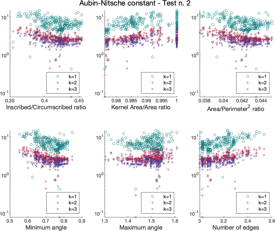
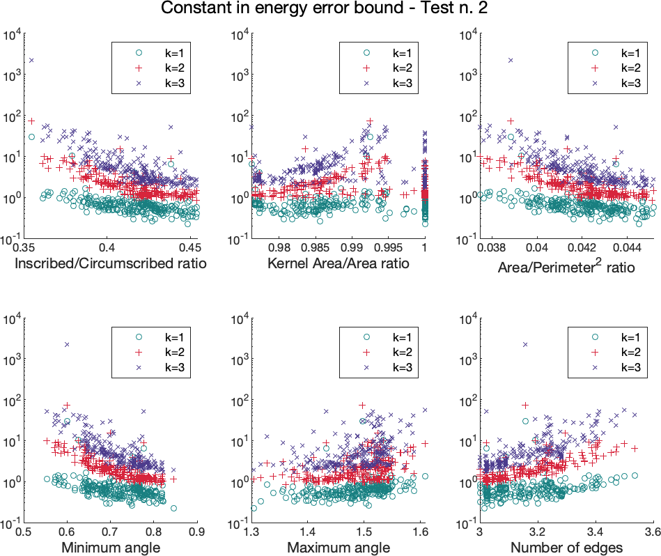
(a)	(b)

Figure 14: Relation between the Aubin-Nitsche constant (a) or the constant in the classical a priori error bound (b) and the scale invariant metrics for $k=1$, $2$ and $3$.

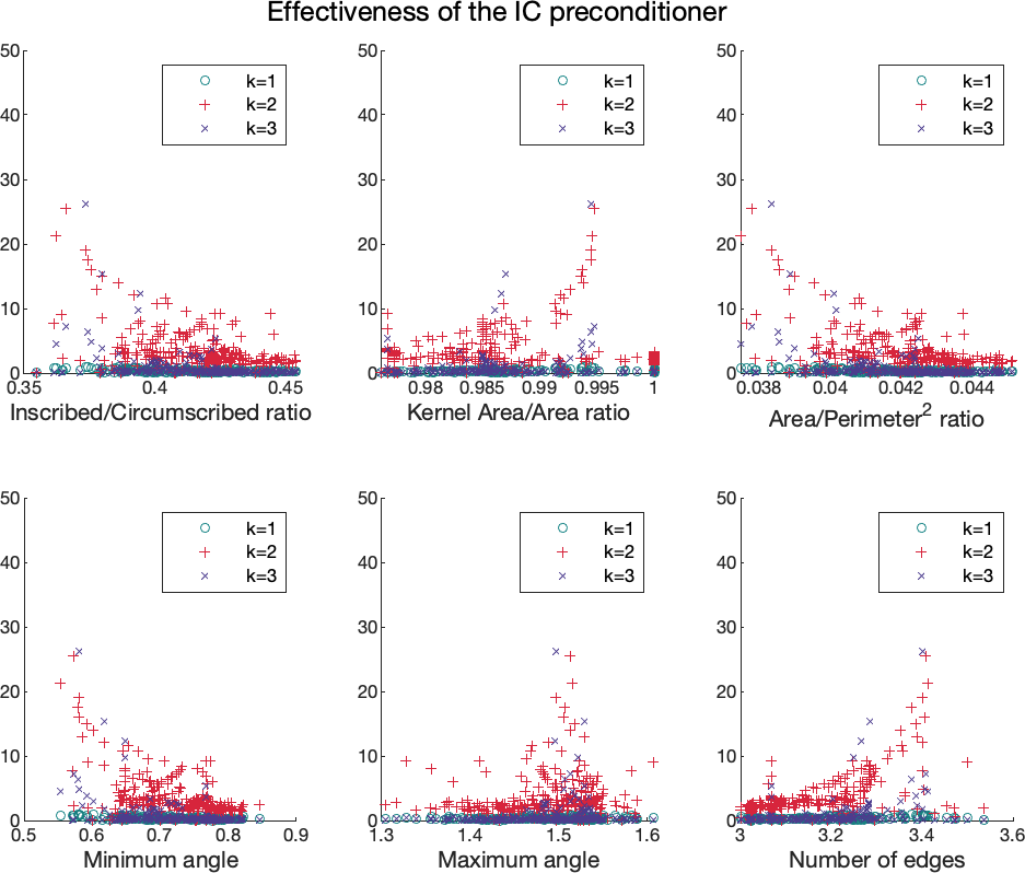
Figure 15: Relation between the effectiveness of the incomplete Choleski preconditioner and the scale invariant metrics for $k=1$, $2$ and $3$.

6 Mesh quality indicators

In this section we define a mesh quality indicator, that is, a scalar function capable of providing insights on the behaviour of the VEM over a particular mesh $\Omega_{h}$, before actually computing the approximated solution $u_{h}$. This indicator depends uniquely on the geometry of the mesh elements, but has interesting correspondences with the performance of the VEM, in terms of approximation error and convergence rate.

6.1 Definition

We start from the geometrical assumptions defined in Section 3.1. The driving idea is that instead of imposing an absolute condition that a mesh can only satisfy or violate, we want to measure how much the mesh satisfies or violate that condition. This approach is more accurate, as it captures small quality differences between meshes, and it does not exclude a priori all the particular cases of meshes only slightly outside the geometrical assumptions.
From each geometrical assumption Gi, i $=1,\ldots,4$, we derive a scalar function $\varrho_{i}:\{E\subset\Omega_{h}\}\to[0,1]$ defined element-wise, which measures how well the element $E\in\Omega_{h}$ meets the requirements of Gi from 0 ($E$ does not respect Gi) to 1 ($E$ fully respects Gi).

From assumption G1 we derive the indicator $\varrho_{1}$, which can be interpreted as an estimate of the value of the constant $\rho$ from G1 on the polygon $E$:

$$\varrho_{1}(E)=\frac{k(E)}{|E|},$$

being $k(E)$ the area of the kernel of a polygon $E$, defined as the set of points in $E$ from which the whole polygon is visible (cf. (KE) of Section 5.1). Therefore, $\varrho_{1}(E)=1$ if $E$ is convex, $\varrho_{1}(E)=0$ if $E$ is not star-shaped and $\varrho_{1}(E)\in(0,1)$ if $E$ is concave but star-shaped.

Similarly, the function $\varrho_{2}$ returns an estimate of the constant $\rho$ introduced in G2, expressed trough the ratio $|e|/h_{E}$:

$$\varrho_{2}(E)=\frac{\min(\sqrt{|E|},\ \min_{e\in\partial E}|e|)}{\max(\sqrt{|E|},\ h_{E})}.$$

The insertion of the quantity $\sqrt{|E|}$ is needed in order to scale the indicator in the range $[0,1]$ and to avoid pathological situations.

Function $\varrho_{3}$ is a simple counter of the number of edges of the polygon, which penalizes elements with numerous edges as required by G3:

$$\varrho_{3}(E)=\frac{3}{\#\left\{e\in\partial E\right\}}.$$

It returns 1 if $E$ is a triangle, and it decreases as the number of edges increases.

Last, we recall from Section 3.1 that the boundary of a polygon $E$ can be considered as a 1-dimensional mesh $\mathcal{I}_{E}$, which can be subdivided into disjoint sub-meshes $\mathcal{I}_{E}^{1},\ldots,\mathcal{I}_{E}^{N}$, each one containing possibly more than one edge of $E$. In practice, we consider as a sub-mesh the collection of all edges whose vertices lie on the same line: an example is shown in Fig. 16.

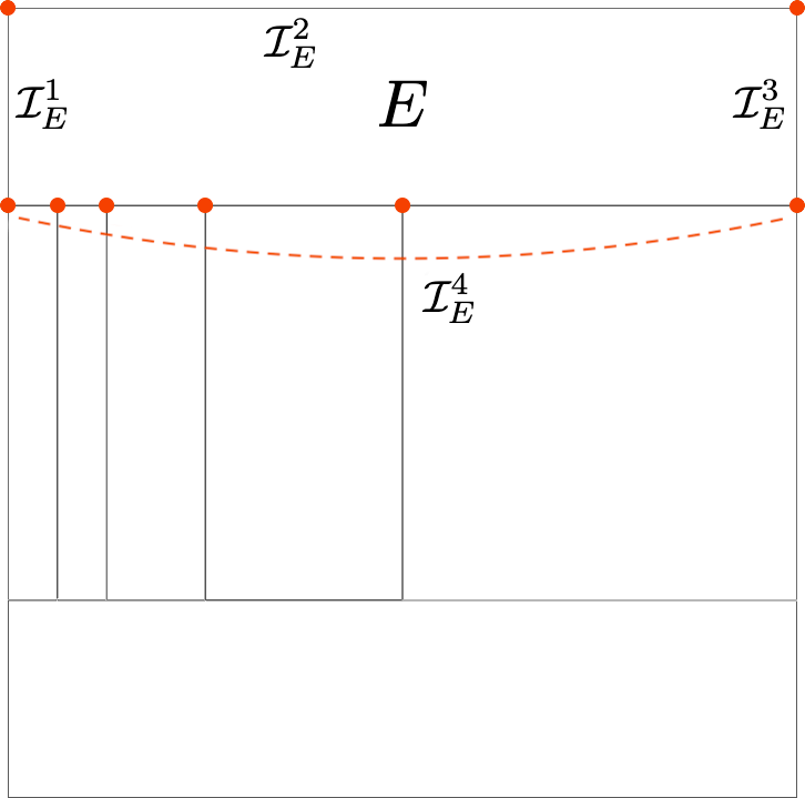
Figure 16: One-dimensional mesh relative to the top bar element $E$ of a $\mathcal{D}_{\rm{Jenga}}$ base mesh. The boundary of $E$ is represented by a mesh $\mathcal{I}_{E}=\{\mathcal{I}_{E}^{1},\mathcal{I}_{E}^{2},\mathcal{I}_{E}^{3},\mathcal{I}_{E}^{4}\}$, where the sub-meshes $\mathcal{I}_{E}^{1},\mathcal{I}_{E}^{2}$ and $\mathcal{I}_{E}^{3}$ contain, respectively, the left, top and right edge of $E$, while $\mathcal{I}_{E}^{4}$ contains all the aligned edges in the bottom of $E$.

The indicator $\varrho_{4}$ returns the minimum ratio between the smallest and the largest element in every $\mathcal{I}_{E}$, that is a measure of the quasi-uniformity of $\mathcal{I}_{E}$ imposed by G4:

$$\varrho_{4}(E)=\min_{i}\frac{\min_{e\in\mathcal{I}_{E}^{i}}|e|}{\max_{e\in\mathcal{I}_{E}^{i}}|e|}.$$

Combining together $\varrho_{1},\varrho_{2}$, $\varrho_{3}$ and $\varrho_{4}$, we define a global function $\varrho:\{\Omega_{h}\}_{h}\to[0,1]$ which measures the overall quality of a mesh $\Omega_{h}$. Given a dataset $\mathcal{D}$, we can study the behaviour of $\varrho(\Omega_{h})$ for $h\to 0$ and determine the quality of the meshes through the refinement process. In particular, we combine the indicators with the formula $\varrho_{1}\varrho_{2}+\varrho_{1}\varrho_{3}+\varrho_{1}\varrho_{4}$ as it reflects the way in which these assumptions are typically imposed: G1 and G2, G1 and G3 or G1 and G4 (but not, for instance, G2 and G3 simultaneously):

$$\varrho(\Omega_{h})=\sqrt{\frac{1}{\#\left\{E\in\Omega_{h}\right\}}\ \sum_{E\in\Omega}\frac{\varrho_{1}(E)\varrho_{2}(E)+\varrho_{1}(E)\varrho_{3}(E)+\varrho_{1}(E)\varrho_{4}(E)}{3}}.$$ (61)

We list some observations on the newly defined mesh quality indicator $\varrho$:

• we have $\varrho(\Omega_{h})=1$ if and only if $\Omega_{h}$ contains only equilateral triangles, $\varrho(\Omega_{h})=0$ if and only if $\Omega_{h}$ contains only non star-shaped polygons, and $0<\varrho(\Omega_{h})<1$ otherwise;

• the indicator $\varrho$ only depends on the geometrical properties of the mesh elements (because the same holds for $\varrho_{1},\varrho_{2}$, $\varrho_{3}$ and $\varrho_{4}$), therefore it can be computed before applying the numerical scheme;

• the construction of $\varrho$ is easily upgradeable to future developments: whenever new assumptions on the features of a mesh should come up, one simply needs to introduce a new function $\varrho_{i}$ that measures the violation of the new assumption and opportunely insert it into equation (61);

• similarly, this indicator is easily extendable to other numerical schemes by substituting the assumptions designed for the VEM with the assumptions on the new scheme, and defining the relative indicators $\varrho_{i}$.

6.2 Results

We evaluated the indicator $\varrho$ over the datasets defined in Section 4.1; results are shown in Fig. 17. We want to investigate if the $\varrho$ values of the meshes of a certain dataset in Fig. 17, computed before solving the problem, are somehow related to the performance of the VEM over the meshes of the same dataset, shown in Fig. 6 and 7, in terms of error approximation and convergence rate.

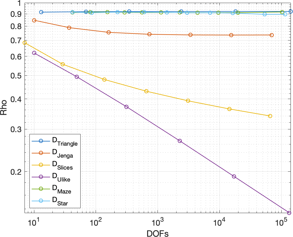
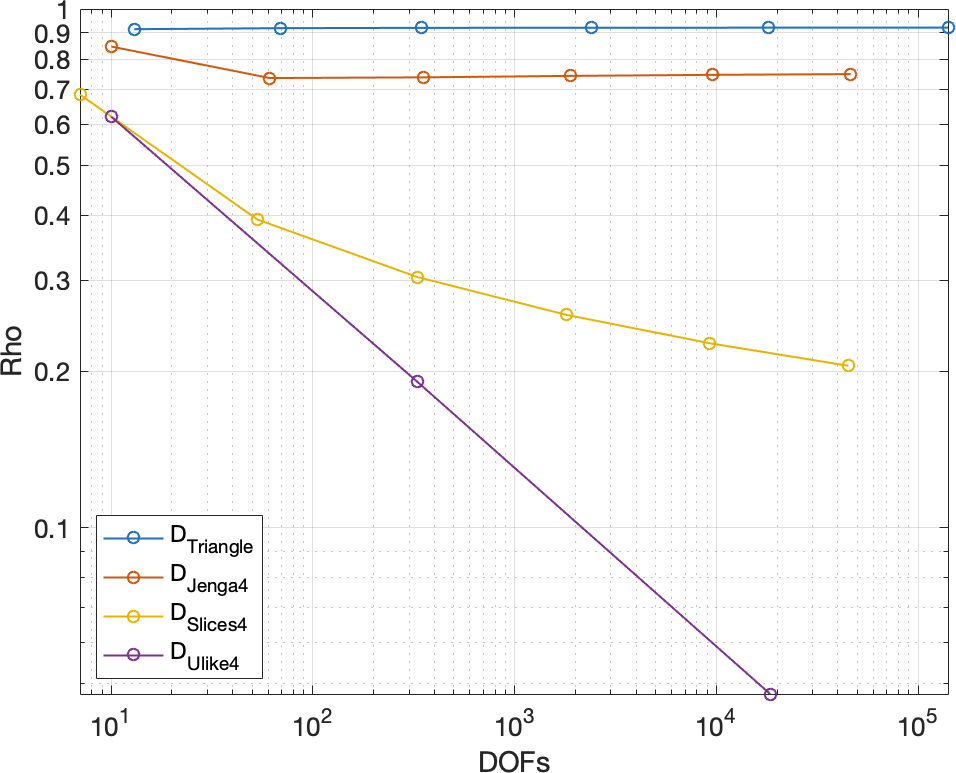
(a)	(b)

Figure 17: Indicator $\varrho$ for all datasets from Section 4.1.

Since $\varrho$ does not depend on the polynomial degree $k$ nor on the type of norm used, we have to consider an hypothetical average of the plots for the different $k$ values and for the different norms ($L^{2}$ and $H^{1}$) from Fig. 6 and 7.
As already seen, for an ideal dataset made by meshes containing only equilateral triangles, $\varrho$ would be constantly equal to 1. We assume this value as a reference for the other datasets: the closer $\varrho$ is on a dataset to the line $y=1$, the smaller is the approximation error that we expect that dataset to produce. Similarly, the more negative is the $\varrho$ slope, the worse is the convergence rate that we expect the method to obtain over that dataset.

For meshes belonging to $\mathcal{D}_{\rm{Triangle}}$, $\varrho$ is almost constant and very close to 1, thus foreseeing the excellent convergence rates and the low errors relative to $\mathcal{D}_{\rm{Triangle}}$ in every sub-figure of Fig. 6.

The plots for $\mathcal{D}_{\rm{Maze}}$ and $\mathcal{D}_{\rm{Star}}$ in Fig. 17(a) are close to the $\mathcal{D}_{\rm{Triangle}}$ one, hence we expect the method to perform similarly over the three of them. This is confirmed by Fig. 6: $\mathcal{D}_{\rm{Maze}}$ and $\mathcal{D}_{\rm{Star}}$ are almost coincident and very close to $\mathcal{D}_{\rm{Triangle}}$ until the very last meshes, especially in the $L^{2}$ plots.

The $\mathcal{D}_{\rm{Jenga}}$ plot in Fig. 17(a) suggests a perfect convergence rate but greater error values with respect to the previous three, and again this behaviour is respected in Fig. 6.
The curve relative to $\mathcal{D}_{\rm{Slices}}$ in Fig. 17(a) is quite distant from the ideal value of 1. Moreover, the curve keeps decreasing from mesh to mesh, even if we may assume that it would flatten within few more meshes. Looking at Fig. 6, we notice that $\mathcal{D}_{\rm{Slices}}$ produces an error significantly higher than the previous ones ($\mathcal{D}_{\rm{Triangle}},\mathcal{D}_{\rm{Maze}},\mathcal{D}_{\rm{Star}},\mathcal{D}_{\rm{Jenga}}$), and in some cases the $H^{1}$ error convergence rate is significantly lower than the theoretical estimate, thus confirming the prediction.
Last, the $\varrho$ values in Fig. 17(a) predict huge errors and a completely wrong convergence rate for $\mathcal{D}_{\rm{Ulike}}$. In fact, this dataset is the one with the worst performance in Fig. 6, where the VEM does not even always converge (for example in the case $k=1$ with the $H^{1}$ seminorm).

As far as multiply refined datasets are concerned, we note that, since $\varrho$ only depends on the geometry of the elements, it is not affected by numerical errors.
The $\varrho$ plot for $\mathcal{D}_{\rm{Jenga4}}$ in Fig. 17(b) is very similar to the one relative to $\mathcal{D}_{\rm{Jenga}}$ in 17(a), therefore we should expect $\mathcal{D}_{\rm{Jenga4}}$ in Fig. 7 to perform similarly to $\mathcal{D}_{\rm{Jenga}}$ in Fig. 6. This is actually the case, at least until the finest mesh for $k=3$ where numerical problems appear which $\varrho$ is not able to predict.
Also $\mathcal{D}_{\rm{Slices4}}$ and $\mathcal{D}_{\rm{Slices}}$ are similar in Fig. 17, but $\varrho$ decreases faster on the first than on the second one, reaching a $\varrho$ value of $\sim 0.2$ instead of $\sim 0.34$ within a smaller number of meshes. Again, this information is correct because the method performs similarly over $\mathcal{D}_{\rm{Slices4}}$ and $\mathcal{D}_{\rm{Slices}}$ until condition numbers explode, in the last two meshes for every value of $k$.
Last, the $\varrho$ plot of $\mathcal{D}_{\rm{Ulike4}}$ is significantly worse than any other (including the one of $\mathcal{D}_{\rm{Ulike}}$), both in terms of distance from $y=1$ and slope. In Fig. 7 we can observe how, even if $\mathcal{D}_{\rm{Ulike4}}$ does not properly explode (as it suffers less from numerical problems, cf. Table 2), the approximation error and the convergence rate are the worst among all the considered datasets.

Summing up these results, we conclude that the indicator $\varrho$ is able, up to a certain accuracy, to predict the behaviour of the VEM over the considered datasets, both in terms of error magnitude and convergence rate. Looking at the $\varrho$ values it is possible to estimate in advance if a mesh or a dataset is going to be more or less critical for the VEM, and it is possible to compare the values relatives to different meshes and datasets to understand which one is going to perform better. The prediction may be less accurate in presence of very similar performance (e.g. the case of $\mathcal{D}_{\rm{Maze}}$ and $\mathcal{D}_{\rm{Star}}$) or in extremely pathological situations, where numerical problems become so significant to overcome any influence that the geometrical features of the mesh may have on the performance (e.g. the last meshes of $\mathcal{D}_{\rm{Jenga4}}$ and $\mathcal{D}_{\rm{Slices4}}$).

7 PEMesh benchmarking tool

Main existing tools for the numerical solution of PDEs include VEMLab [52], which is an open source MATLAB library for the virtual element method and Veamy, which is a free and open source C++ library that implements the virtual element method (C++ version of [52]). This library allows the user to solve 2D linear elasto-static problems and the 2D Poisson problem [51]. Additional tools include the 50-lines MATLAB implementation of the lowest order virtual element method for the two-dimensional Poisson problem on general polygonal meshes [61] and the MATLAB implementation of the lowest order Virtual Element Method (VEM) [48].

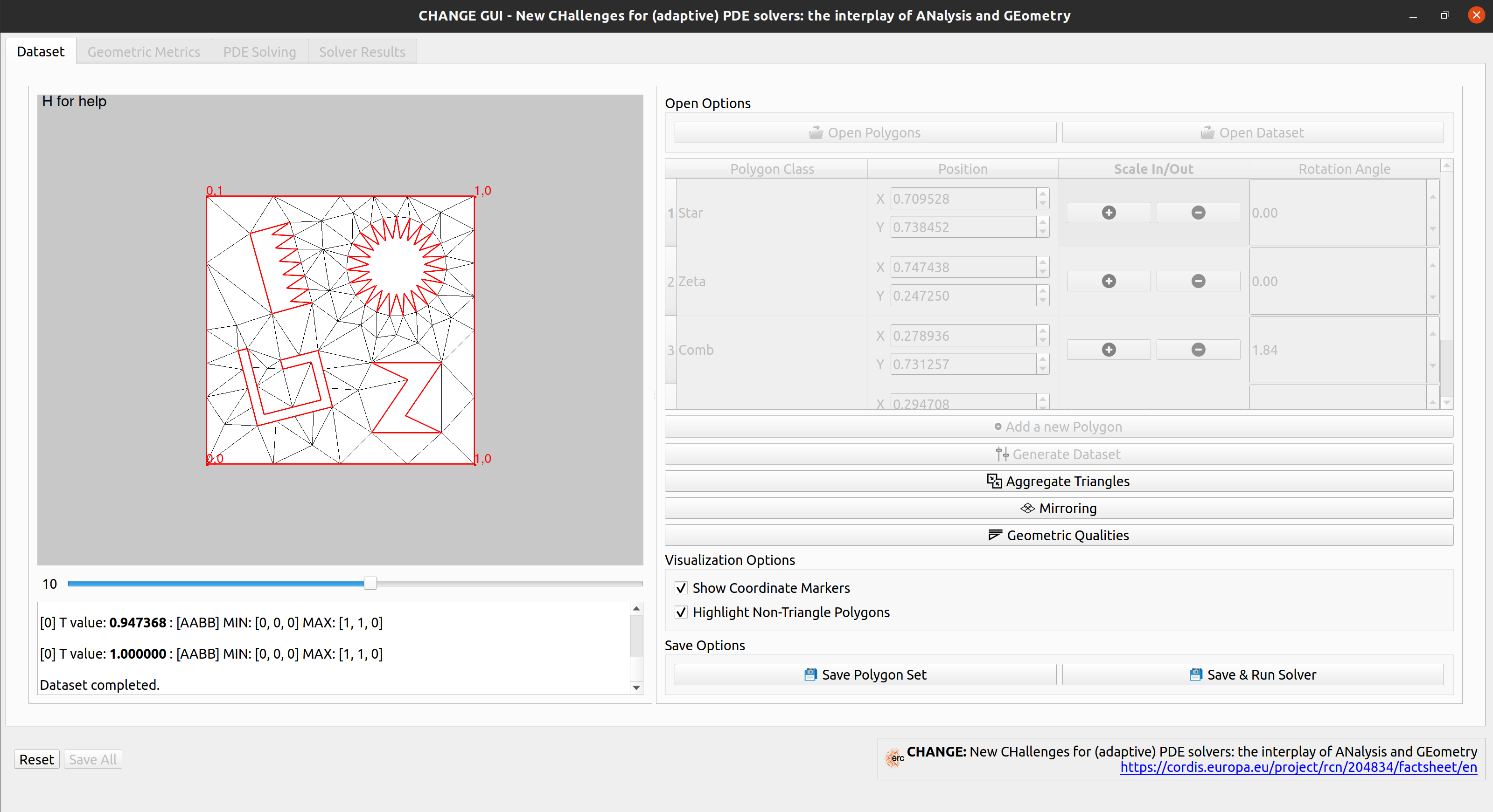
(a)

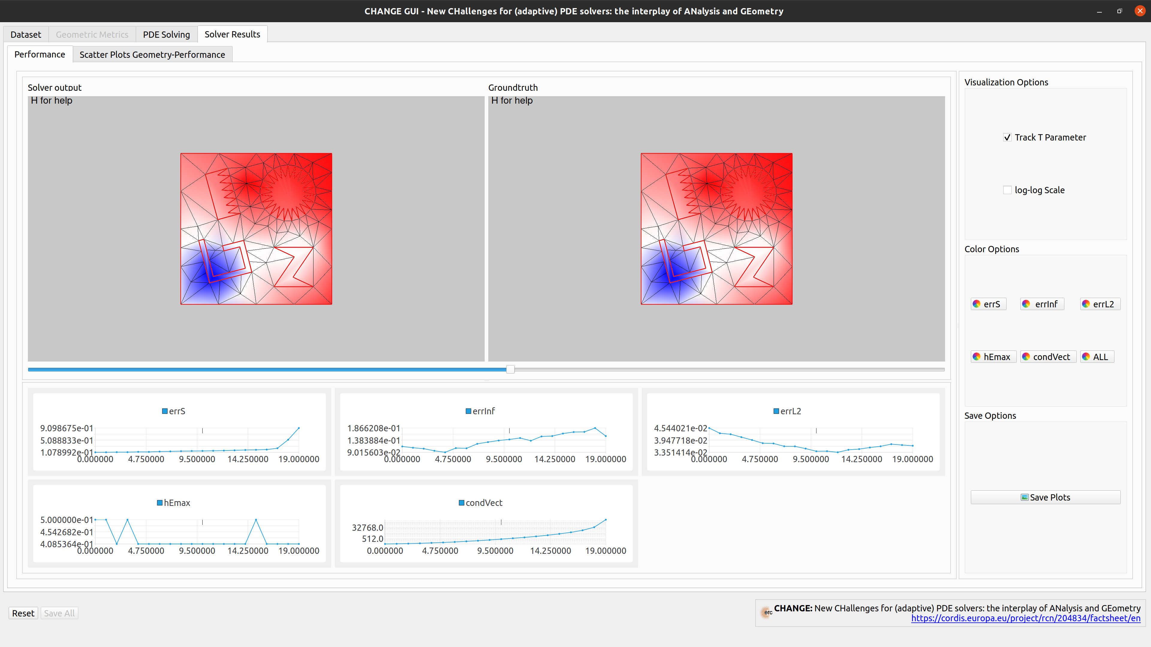
(b)

Figure 18: (a) Main window of PEMesh and (b) examples of PEM solver results. On the top, both solver output and ground truth are color-mapped on the input polygon meshes, while on the bottom a set of linear plots show how solver performances vary in the data set.

In this context, PEMesh [29] (Fig. 18) is an open-source software tool for experiments on the analysis and design of polytopal meshes for PEM solvers. PEMesh is an advanced graphical tool that seamless integrates the geometric design of 2D domains and PEM simulations. It supports the design and generation of complex input polygonal meshes by stressing geometric properties and provides the possibility to solve PEMs on the generated meshes. Furthermore, PEMesh allows us to correlate several geometric properties of the input polytopal mesh with the performances of PEM solvers, and to visualise the results though customisable and interactive plots. PEMesh also supports to evaluate the dependence of the performances of a PEM solver on geometrical properties of the input polygonal mesh. PEMesh includes four main modules, which are briefly described in the following.

Polygon mesh generation $\&$ loading allow us to load one or more existing meshes or to generate new ones from scratch by either exploiting a set of polytopal elements available in the module or providing an external polytopal element. In this way, the user can easily generate a large set of options and parameters.
We used this module for the generation of most of the datasets considered in this work: $\mathcal{D}_{\rm{Triangle}},\mathcal{D}_{\rm{Star}},\mathcal{D}_{\rm{Maze}}$ and all datasets from Section 5.3. The mirroring and multiple mirroring datasets defined in Section 4.1 have been generated separately and then loaded into the software to be used in the subsequent modules.

Geometric analysis allows the user to perform a deep analysis of geometric properties of the input polygonal meshes, to correlate each of them with the others, and to visualise the results of this analysis though scatter plots (see Fig. 19(a)).

PEM solver allows the user to run a PEM solver and to analyse its performances on input polygonal meshes. Any PEM solver, which is run from command line, can be integrated in the software together with its output. The PEM and ground-through (if any) solutions of the PEM are shown directly on the meshes, while the performances of the solver are visualized through linear plots.
This module has been used for solving the problem and analyzing the performance of the VEM over all datasets in this work.

Correlation visualization allows the user to analyse the correlation between geometric properties of the polygonal meshes and numerical performances of the PEM solver. Then, the results are visualised as customizable scatter plots, as shown in Fig. 19(b).

PEMesh provides the possibility to solve PEMs on a polygonal mesh and to visualize the performances of any PEM solver. To this end, the PEM solver is not part of the tool, but is handled as an external resource that is called by PEMesh graphical interface. Through a general approach, PEMesh assumes that the selected PEM solver takes an input mesh and returns both the solution and the ground-truth (if any) of a PDE, together with statistics (e.g., approximation accuracy, condition number of the mass and stiffness matrices) of the PEM solver. Then, the results of the PEM solver are visualised in a specialized window, and the numerical and geometric metrics are shown as linear plots (Fig. 18b). Finally, a set of visualization options are available for the customisation of color-maps and linear plots. Through a modular and customisable system, PEMesh allows us to run any PEM solver, thus providing an easy way to generate complex discrete polytopal meshes and to study the correlation between geometric properties of the input mesh and numerical PEMs solvers.

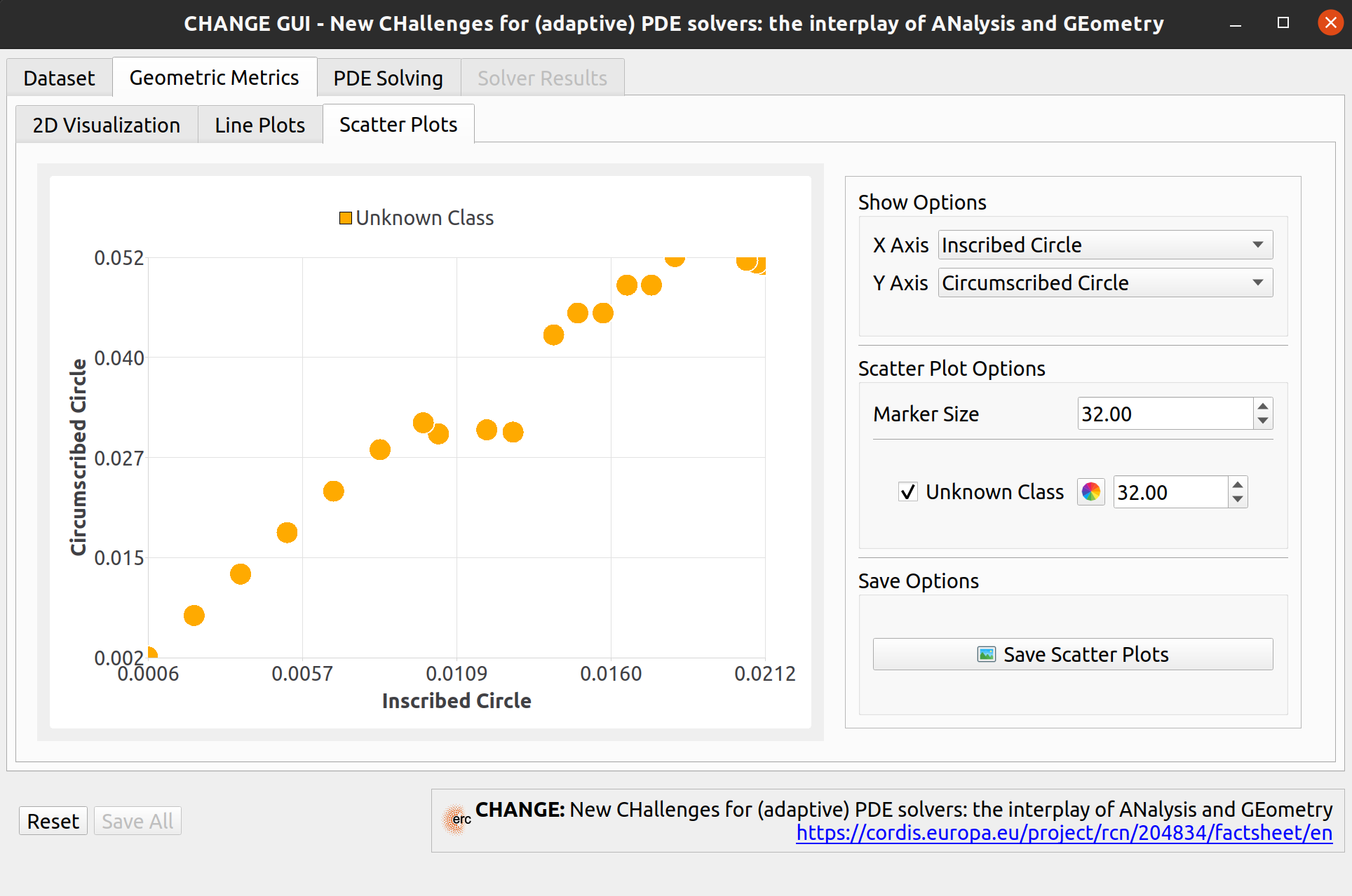
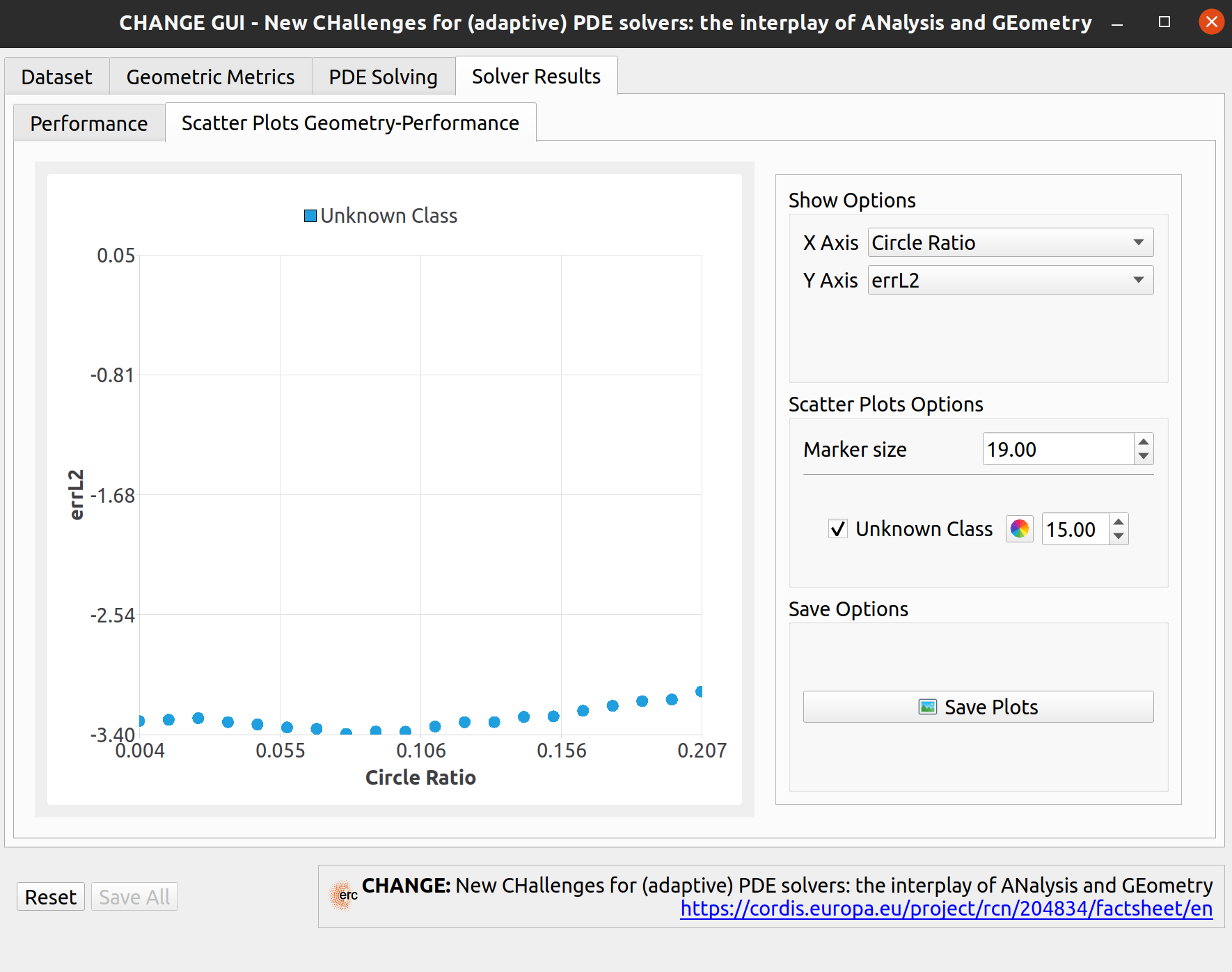
(a)	(b)

Figure 19: PEMesh window specialized on the visualization of the correlation between geometric metrics (a) and the correlation of geometric metrics and PEM performances (b). The right side of the window provides some visualization options to enable the possibility to select which metrics to be visualized and how (i.e. size, color, …).

References

- [1] B. Ahmad, A. Alsaedi, F. Brezzi, L. D. Marini, and A. Russo. Equivalent projectors for virtual element methods. Computers & Mathematics with Applications, 66:376–391, September 2013.
- [2] P. F. Antonietti, L. Beirão da Veiga, S. Scacchi, and M. Verani. A virtual element method for the Cahn-Hilliard equation with polygonal meshes. SIAM Journal on Numerical Analysis, 54(1):34–56, 2016.
- [3] P. F. Antonietti, G. Manzini, and M. Verani. The conforming virtual element method for polyharmonic problems. Computers & Mathematics with Applications, 2019. published online: 4 October 2019.
- [4] P. F. Antonietti, L. Mascotto, and M. Verani. A multigrid algorithm for the -version of the virtual element method. ESAIM: Math. Model. Numer. Anal., 52(1):337–364, 2018.
- [5] L. Beirão da Veiga, F. Brezzi, A. Cangiani, G. Manzini, L. D. Marini, and A. Russo. Basic principles of virtual element methods. Mathematical Models & Methods in Applied Sciences, 23:119–214, 2013.
- [6] L. Beirão da Veiga, F. Brezzi, L. D. Marini, and A. Russo. The Hitchhiker’s guide to the virtual element method. Mathematical Models and Methods in Applied Sciences, 24(8):1541–1573, 2014.
- [7] L. Beirão da Veiga, F. Brezzi, L. D. Marini, and A. Russo. H(div) and H(curl)-conforming VEM. Numerische Mathematik, 133(2):303–332, 2016.
- [8] L. Beirão da Veiga, F. Brezzi, L. D. Marini, and A. Russo. Virtual element methods for general second order elliptic problems on polygonal meshes. Mathematical Models & Methods in Applied Sciences, 26(4):729–750, 2016.
- [9] L. Beirão da Veiga, A. Chernov, L. Mascotto, and A. Russo. Basic principles of hp virtual elements on quasiuniform meshes. Mathematical Models & Methods in Applied Sciences, 26(8):1567–1598, 2016.
- [10] L. Beirão da Veiga, K. Lipnikov, and G. Manzini. Arbitrary order nodal mimetic discretizations of elliptic problems on polygonal meshes. SIAM Journal on Numerical Analysis, 49(5):1737–1760, 2011.
- [11] L. Beirão da Veiga, K. Lipnikov, and G. Manzini. The Mimetic Finite Difference Method, volume 11 of MS&A. Modeling, Simulations and Applications. Springer, I edition, 2014.
- [12] L. Beirão da Veiga and G. Manzini. A virtual element method with arbitrary regularity. IMA Journal on Numerical Analysis, 34(2):782–799, 2014. DOI: 10.1093/imanum/drt018, (first published online 2013).
- [13] L. Beirão da Veiga and G. Manzini. Residual a posteriori error estimation for the virtual element method for elliptic problems. ESAIM: Mathematical Modelling and Numerical Analysis, 49:577–599, 2015.
- [14] L. Beirão da Veiga, G. Manzini, and M. Putti. Post-processing of solution and flux for the nodal mimetic finite difference method. Numerical Methods for Partial Differential Equations, 31(1):336–363, 2015.
- [15] L. Beirão da Veiga and G. Vacca. Sharper error estimates for virtual elements and a bubble-enriched version. arXiv preprint arXiv:2005.12009, 2020.
- [16] L. Beirão da Veiga, A. Chernov, L. Mascotto, and A. Russo. Exponential convergence of the virtual element method in presence of corner singularities. Numerische Mathematik, 138(3):581–613, 2018.
- [17] L. Beirão da Veiga, C. Lovadina, and A. Russo. Stability analysis for the virtual element method. Mathematical Models and Methods in Applied Sciences, 27(13):2557–2594, 2017.
- [18] M. F. Benedetto, S. Berrone, S. Pieraccini, and S. Scialò. The virtual element method for discrete fracture network simulations. Computer Methods in Applied Mechanics and Engineering, 280(0):135 – 156, 2014.
- [19] E. Benvenuti, A. Chiozzi, G. Manzini, and N. Sukumar. Extended virtual element method for the Laplace problem with singularities and discontinuities. Computer Methods in Applied Mechanics and Engineering, 356:571 – 597, 2019.
- [20] S. Berrone, S. Pieraccini, S. Scialò, and F. Vicini. A parallel solver for large scale DFN flow simulations. SIAM Journal on Scientific Computing, 37(3):C285–C306, 2015.
- [21] S. Bertoluzza, G. Manzini, M. Pennacchio, and D. Prada. Stabilization of the nonconforming virtual element method. arXiv.XXX.XXXXXXX, 2021. (submitted).
- [22] S. Bertoluzza, M. Pennacchio, and D. Prada. BDDC and FETI-DP for the virtual element method. Calcolo, 54(4):1565–1593, Dec 2017.
- [23] S. Bertoluzza, M. Pennacchio, and D. Prada. FETI-DP for the three dimensional virtual element method. SIAM Journal Numerical Analysis, 58, 2020.
- [24] J. Brandts, S. Korotov, and M Krizek. On the equivalence of regularity criteria for triangular and tetrahedral finite element partitions. Computers & Mathematics with Applications, 55, 2008.
- [25] S. C. Brenner, Q. Guan, and L.-Y. Sung. Some estimates for virtual element methods. Computational Methods in Applied Mathematics, 17(4):553–574, 2017.
- [26] S. C. Brenner and L.-Y. Sung. Virtual element methods on meshes with small edges or faces. Mathematical Models and Methods in Applied Sciences, 28(07):1291–1336, 2018.
- [27] F. Brezzi, A. Buffa, and K. Lipnikov. Mimetic finite differences for elliptic problems. M2AN Math. Model. Numer. Anal., 43:277–295, 2009.
- [28] R. Bridson. Fast Poisson disk sampling in arbitrary dimensions. SIGGRAPH sketches, 10:1, 2007.
- [29] D. Cabiddu, G. Patanè, and M. Spagnuolo. PEMesh: Graphical framework for the analysis of the interplay between geometry and PEM solvers. Arxiv https://arxiv.org/abs/2102.11578, 2021.
- [30] J. G. Calvo. An overlapping Schwarz method for virtual element discretizations in two dimensions. Comput. Math. Appl., 77(4):1163–1177, 2019.
- [31] A. Cangiani, E. H. Georgoulis, T. Pryer, and O. J. Sutton. A posteriori error estimates for the virtual element method. Numerische Mathematik, pages 1–37, 2017.
- [32] A. Cangiani, V. Gyya, G. Manzini, and Sutton. O. Chapter 14: Virtual element methods for elliptic problems on polygonal meshes. In K. Hormann and N. Sukumar, editors, Generalized Barycentric Coordinates in Computer Graphics and Computational Mechanics, pages 1–20. CRC Press, Taylor & Francis Group, 2017.
- [33] A. Cangiani, G. Manzini, A. Russo, and N. Sukumar. Hourglass stabilization of the virtual element method. International Journal on Numerical Methods in Engineering, 102(3-4):404–436, 2015.
- [34] O. Certik, F. Gardini, G. Manzini, L. Mascotto, and G. Vacca. The p- and hp-versions of the virtual element method for elliptic eigenvalue problems, 2020.
- [35] O. Certik, F. Gardini, G. Manzini, and G. Vacca. The virtual element method for eigenvalue problems with potential terms on polytopic meshes. Applications of Mathematics, 63(3):333–365, 2018.
- [36] L. Chen and J. Huang. Some error analysis on virtual element methods. Calcolo, 55, 2018.
- [37] C. Chinosi and L. D. Marini. Virtual element method for fourth order problems: L2-estimates. Computers & Mathematics with Applications, 72(8):1959 – 1967, 2016. Finite Elements in Flow Problems 2015.
- [38] P. G. Ciarlet. The finite element method for elliptic problems. SIAM, 2002.
- [39] F. Dassi and L. Mascotto. Exploring high-order three dimensional virtual elements: bases and stabilizations. Comput. Math. Appl., 75(9):3379–3401, 2018.
- [40] D. A. Di Pietro, J. Droniou, and G. Manzini. Discontinuous skeletal gradient discretisation methods on polytopal meshes. Journal of Computational Physics, 355:397–425, 2018.
- [41] G.H. Golub and C.F. Van Loan. Matrix Computations (3rd ed.). Johns Hopkins, 1996.
- [42] W.W. Hager. Condition estimates. SIAM Journal Scientific Statistical Computing, 5, 1984.
- [43] N.J. Higham and F. Tisseur. A block algorithm for matrix 1-norm estimation with an application to 1-norm pseudospectra. SIAM Journal Matrix Analysis Applications, 21, 2000.
- [44] K. Lipnikov, G. Manzini, and M. Shashkov. Mimetic finite difference method. Journal of Computational Physics, 257 – Part B:1163–1227, 2014. Review paper.
- [45] M. Livesu. cinolib: a generic programming header only C++ library for processing polygonal and polyhedral meshes. In Transactions on Computational Science XXXIV, pages 64–76. Springer, 2019.
- [46] G. Manzini, K. Lipnikov, J. D. Moulton, and M. Shashkov. Convergence analysis of the mimetic finite difference method for elliptic problems with staggered discretizations of diffusion coefficients. SIAM Journal on Numerical Analysis, 55(6):2956–2981, 2017.
- [47] G. Manzini, A. Russo, and N. Sukumar. New perspectives on polygonal and polyhedral finite element methods. Mathematical Models & Methods in Applied Sciences, 24(8):1621–1663, 2014.
- [48] L. Mascotto. Ill-conditioning in the virtual element method: stabilizations and bases. Numer. Methods Partial Differential Equations, 34(4):1258–1281, 2018.
- [49] D. Mora, G. Rivera, and R. Rodríguez. A virtual element method for the Steklov eigenvalue problem. Mathematical Models and Methods in Applied Sciences, 25(08):1421–1445, 2015.
- [50] J.L. Myers and A.D. Well. Research Design and Statistical Analysis (2nd ed.). Lawrence Erlbaum., 2003.
- [51] A. Ortiz-Bernardin, C. Alvarez, N. Hitschfeld-Kahler, A. Russo, R. Silva-Valenzuela, and E. Olate-Sanzana. Veamy: an extensible object-oriented C++ library for the virtual element method. Numerical Algorithms, 82(4):1189–1220, 2019.
- [52] A. Ortiz-Bernardin, C. Alvarez, N. Hitschfeld-Kahler, A. Russo, R. Silva-Valenzuela, and E. Olate-Sanzana. VEMLab: a MATLAB library for the virtual element method. https://github.com/cemcen/vemlab, 2020.
- [53] G. H. Paulino and A. L. Gain. Bridging art and engineering using Escher-based virtual elements. Structures and Multidisciplinary Optimization, 51(4):867–883, 2015.
- [54] I. Perugia, P. Pietra, and A. Russo. A plane wave virtual element method for the Helmholtz problem. ESAIM: Mathematical Modelling and Numerical Analysis, 50(3):783–808, 2016.
- [55] L. Ridgway Scott and S. C. Brenner. The mathematical theory of finite element methods. Texts in applied mathematics 15. Springer-Verlag New York, 3 edition, 2008.
- [56] J. R. Shewchuk. Triangle: Engineering a 2d quality mesh generator and delaunay triangulator. In Selected Papers from the Workshop on Applied Computational Geormetry, Towards Geometric Engineering, FCRC ’96/WACG ’96, page 203–222, Berlin, Heidelberg, 1996. Springer-Verlag.
- [57] J. R. Shewchuk. What is a good linear finite element? - interpolation, conditioning, anisotropy, and quality measures. Technical report, In Proc. of the 11th International Meshing Roundtable, 2002.
- [58] L. Simonson and G. Suto. Geometry template library for stl-like 2d operations. Colorado: GTL Boostcon, 2009.
- [59] T. Sorgente, S. Biasotti, G. Manzini, and M. Spagnuolo. The role of mesh quality and mesh quality indicators in the virtual element method, 2021.
- [60] C. Spearman. The proof and measurement of association between two things. Journal of Psychology, 15, 1904.
- [61] O. J. Sutton. The Virtual Element Method in 50 Lines of MATLAB. Numer. Algorithms, 75(4):1141–1159, August 2017.
- [62] E. Welzl. Smallest enclosing disks (balls and ellipsoids). In New results and new trends in computer science, pages 359–370. Springer, 1991.
- [63] P. Wriggers, W. T. Rust, and B. D. Reddy. A virtual element method for contact. Computational Mechanics, 58(6):1039–1050, 2016.
- [64] M. Zlámal. On the finite element method. Numerische Mathematik, 12(5):394–409, 1968.