Continuous Record Asymptotic Framework for Inference in Strucutral Change Models

Theory of Low Frequency Contamination from Nonstationarity and Misspecification: Consequences for HAR Inference

Abstract

We establish theoretical results about the low frequency contamination (i.e., long memory effects) induced by general nonstationarity for estimates such as the sample autocovariance and the periodogram, and deduce consequences for heteroskedasticity and autocorrelation robust (HAR) inference. We present explicit expressions for the asymptotic bias of these estimates. We distinguish cases where this contamination only occurs as a small-sample problem and cases where the contamination continues to hold asymptotically. We show theoretically that nonparametric smoothing over time is robust to low frequency contamination. Our results provide new insights on the debate between consistent versus inconsistent long-run variance (LRV) estimation. Existing LRV estimators tend to be inflated when the data are nonstationary. This results in HAR tests that can be undersized and exhibit dramatic power losses. Our theory indicates that long bandwidths or fixed-$b$ HAR tests suffer more from low frequency contamination relative to HAR tests based on HAC estimators, whereas recently introduced double kernel HAC estimators do not suffer from this problem. Finally, we present second-order Edgeworth expansions under nonstationarity about the distribution of HAC and DK-HAC estimators and about the corresponding $t$-test in the linear regression model.

Abstract

This supplemental material is for online publication only. It introduces the notion of long memory segmented locally stationary processes in Section S.A. Section S.B contains the proofs of the results in the paper and Section S.C contains additional figures.

JEL Classification: C12, C13, C18, C22, C32, C51
Keywords: Edgeworth expansions, Fixed-$b$, HAC standard errors, HAR, Long memory, Long-run variance, Low frequency contamination, Nonstationarity, Outliers, Segmented locally stationary.

1 Introduction

Economic and financial time series are highly nonstationary [see, e.g., Perron (1989), Stock and Watson (1996), Ng and Wright (2013), and Giacomini and Rossi (2015)]. We develop theoretical results about the behavior of the sample autocovariance ($\widehat{\Gamma}\left(k\right),\,k\in\mathbb{Z}$) and the periodogram ($I_{T}\left(\omega\right),\,\omega\in\left[-\pi,\,\pi\right]$) for a short memory nonstationary process. We show that nonstationarity (e.g., time-variation in the mean or autocovariances) induces low frequency contamination, meaning that the sample autocovariance and the periodogram share features that are similar to those of a long memory series. We present explicit expressions for the asymptotic bias of these estimates, showing that it is always positive and increases with the degree of heterogeneity in the data.

The low frequency contamination can be explained as follows. For a short memory series, the autocorrelation function (ACF) displays exponential decay and vanishes as the lag length $k\rightarrow\infty$, and the periodogram is finite at the origin. Under general forms of nonstationarity, we show theoretically that $\widehat{\Gamma}\left(k\right)=\lim_{T\rightarrow\infty}\Gamma_{T}\left(k\right)+d^{*},$ where $\Gamma_{T}\left(k\right)=T^{-1}\sum_{t=k+1}^{T}\mathbb{E}\left(V_{t}V_{t-k}\right)$, $k\geq 0$ and $d^{*}>0$ is independent of $k$. Assuming positive dependence for simplicity (i.e., $\lim_{T\rightarrow\infty}\Gamma_{T}\left(k\right)>0$), this means that each sample autocovariance overestimates the true dependence in the data. The bias factor $d^{*}>0$ depends on the type of nonstationarity and in general does not vanish as $T\rightarrow\infty$. In addition, since short memory implies $\Gamma_{T}\left(k\right)\rightarrow 0$ as $k\rightarrow\infty$, it follows that $d^{*}$ generates long memory effects since $\widehat{\Gamma}\left(k\right)\thickapprox d^{*}>0$ as $k\rightarrow\infty$. As for the periodogram, $I_{T}\left(\omega\right)$, we show that under nonstationarity $\mathbb{E}\left(I_{T}\left(\omega\right)\right)\rightarrow\infty$ as $\omega\rightarrow 0$, a feature also shared by long memory processes.

This low frequency contamination holds as an asymptotic approximation. We verify analytically the quality of the approximation to finite-sample situations. We distinguish cases where this contamination only occurs as a small-sample problem and cases where it continues to hold asymptotically. The former involves $d^{*}\thickapprox 0$ asymptotically but a consistent estimate of $d^{*}$ satisfies $\widehat{d}^{*}>0$ in finite-sample. We show analytically that using $\widehat{d}^{*}$ in place of $d^{*}$ provides a good approximation in this context. This helps us to explain the long memory effects in situations where asymptotically no low frequency contamination should occur. An example is a $t$-test on a regression coefficient in a correctly specified model with nonstationary errors that are serially correlated. Other examples include $t$-tests in the linear model with mild forms of misspecification that do not undermine the conditions for consistency of the least-squares estimator. Further, similar issues arise if one applies some prior de-trending techniques where the fitted model is not correctly specified (e.g., the data follow a nonlinear trend but one removes a linear trend). Yet another example for which our results are relevant is the case of outliers. In all these examples, $d^{*}\thickapprox 0$ asymptotically but one observes enhanced persistence in finite-samples that can affect the properties of heteroskedasticity and autocorrelation robust (HAR) inference. Most of the HAR inference in applied work (besides the $t$- and $F$-test in regression models) are characterized by nonstationary alternative hypotheses for which $d^{*}>0$ even asymptotically. This class of tests is very large. Tests for forecast evaluation [e.g., Casini (2018), Diebold and Mariano (1995), Giacomini and Rossi (2009, 2010), Giacomini and White (2006), Perron and Yamamoto (2021) and West (1996)], tests and inference for structural change models [e.g., Andrews (1993), Bai and Perron (1998), Casini and Perron (2021c, 2020, 2021b), Elliott and Müller (2007), and Qu and Perron (2007)], tests and inference in time-varying parameters models [e.g., Cai (2007) and Chen and Hong (2012)], tests and inference for regime switching models [e.g., Hamilton (1989) and Qu and Zhuo (2020)] and others are part of this class.

Recently, Casini (2021c) proposed a new HAC estimator that applies nonparametric smoothing over time in order to account flexibly for nonstationarity. We show theoretically that nonparametric smoothing over time is robust to low frequency contamination and prove that the resulting sample local autocovariance and the local periodogram do not exhibit long memory features. Nonparametric smoothing avoids mixing highly heterogeneous data coming from distinct nonstationary regimes as opposed to what the sample autocovariance and the periodogram do.

Our work is different from the literature on spurious persistence caused by the presence of level shifts or other deterministic trends. Perron (1990) showed that the presence of breaks in mean often induces spurious non-rejection of the unit root hypothesis, and that the presence of a level shift asymptotically biases the estimate of the AR coefficient towards one. Bhattacharya et al. (1983) demonstrated that certain deterministic trends can induce the spurious presence of long memory. In other contexts, similar issues were discussed by Christensen and Varneskov (2017), Diebold and Inoue (2001), Demetrescu and Salish (2020), Lamoureux and Lastrapes (1990), Hillebrand (2005), Granger and Hyung (2004), McCloskey and Hill (2017), Mikosch and Stărica (2004) and Perron and Qu (2010). Our results are different from theirs in that we consider a more general problem and we allow for more general forms of nonstationarity using the segmented locally stationary framework of Casini (2021c). Importantly, we provide a general solution to these problems and show theoretically its robustness to low frequency contamination. Moreover, we discuss in detail the implications of our theory for HAR inference.

HAR inference relies on estimation of the long-run variance (LRV). The latter, from a time domain perspective, is equivalent to the sum of all autocovariances while from a frequency domain perspective, is equal to $2\pi$ times an integrated time-varying spectral density at the zero frequency. From a time domain perspective, estimation involves a weighted sum of the sample autocovariances, while from a frequency domain perspective estimation is based on a weighted sum of the periodogram ordinates near the zero frequency. Therefore, our results on low frequency contamination for the sample autocovariances and the periodogram can have important implications.

There are two main approaches in HAR inference which relies on whether the LRV estimator is consistent or not. The classical approach relies on consistency which results in HAC standard errors [cf. Newey and West (1987, 1994) and Andrews (1991)]. Inference is standard because HAR test statistics follow asymptotically standard distributions. It was shown early that HAC standard errors can result in oversized tests when there is substantial temporal dependence. This stimulated a second approach based on inconsistent LRV estimators that keep the bandwidth at a fixed fraction of the sample size [cf. Kiefer et al. (2000)]. Inference becomes nonstandard and it is shown that fixed-$b$ achieves high-order refinements [e.g., Sun et al. (2008)] and reduces the oversize problem of HAR tests. However, unlike the classical approach, current fixed-$b$ HAR inference is only valid under stationarity [cf. Casini (2021b)].

Recent work by Casini (2021c) questioned the performance of HAR inference tests under nonstationarity from a theoretical standpoint. Simulation evidence of serious (e.g., non-monotonic) power or related issues in specific HAR inference contexts were documented by Altissimo and Corradi (2003), Casini (2018), Casini and Perron (2019, 2021c, 2020), Chan (2020), Chang and Perron (2018), Crainiceanu and Vogelsang (2007), Deng and Perron (2006), Juhl and Xiao (2009), Kim and Perron (2009), Martins and Perron (2016), Otto and Breitung (2021), Perron and Yamamoto (2021), Shao and Zhang (2010), Vogelsang (1999) and Zhang and Lavitas (2018) among others]. Our theoretical results show that these issues occur because the unaccounted nonstationarity alters the spectrum at low frequencies. Each sample autocovariance is upward biased ($d^{*}>0$) and the resulting LRV estimators tend to be inflated. When these estimators are used to normalize test statistics, the latter lose power. Interestingly, $d^{*}$ is independent of $k$ so that the more lags are included the more severe is the problem. Further, by virtue of weak dependence, we have that $\Gamma_{T}\left(k\right)\rightarrow 0$ as $k\rightarrow\infty$ but $d^{*}>0$ across $k$. For these reasons, long bandwidths/fixed-$b$ LRV estimators are expected to suffer most because they use many/all lagged autocovariances.

To precisely analyze the theoretical properties of the HAR tests under the null hypothesis, we present second-order Edgeworth expansions under nonstationarity for the distribution of the HAC and DK-HAC estimator and for the distribution of the corresponding $t$-test in the linear regression model. Under stationarity the results concerning the HAC estimator were provided by Velasco and Robinson (2001). We show that the order of the approximation error of the expansion is the same as under stationarity from which it follows that the error in rejection probability (ERP) is also the same. The ERP of the $t$-test based on the DK-HAC estimator is slightly larger than that of the $t$-test based on the HAC estimator due to the double smoothing. High-order asymptotic expansions for spectral and other estimates were studied by Bhattacharya and Ghosh (1978), Bentkus and Rudzkis (1982), Janas (1994), Phillips (1977; 1980) and Taniguchi and Puri (1996). The asymptotic expansions of the fixed-$b$ HAR tests under stationarity were developed by Jansson (2004) and Sun et al. (2008). Casini (2021b) showed that under nonstationarity the ERP of the fixed-$b$ HAR tests can be larger than that of HAR tests based on HAC and DK-HAC estimators thereby controverting the mainstream conclusion in the literature that fixed-$b$ HAR tests are theoretically superior to HAR tests based on consistent LRV estimators.

The paper is organized as follows. Section 2 presents the statistical setting and Section 3 establishes the theoretical results on low frequency contamination. Section 4 presents the Edgeworth expansions of HAR tests based on the HAC and DK-HAC estimators. The implications of our results for HAR inference are analyzed analytically and computationally through simulations in Section 5. Section 6 concludes. The supplemental materials [cf. Casini et al. (2021)] contain some additional examples and all mathematical proofs. The code to implement our method is provided in $\mathrm{\mathsf{Matlab}}$, $\mathrm{\mathrm{\mathsf{R}}}$ and $\mathrm{\mathrm{\mathsf{Stata}}}$ languages through a $\mathrm{\mathrm{\mathsf{Github}}}$ repository.

2 Statistical Framework for Nonstationarity

Suppose $\{V_{t,T}\}_{t=1}^{T}$ is defined on a probability space $\left(\Omega,\,\mathscr{F},\,\mathbb{P}\right)$, where $\Omega$ is the sample space, $\mathscr{F}$ is the $\sigma$-algebra and $\mathbb{P}$ is a probability measure. In order to analyze time series models that have a time-varying spectrum it is useful to introduce an infill asymptotic setting whereby we rescale the original discrete time horizon $\left[1,\,T\right]$ by dividing each $t$ by $T.$ Letting $u=t/T$ we define a new time scale $u\in\left[0,\,1\right]$ on which as $T\rightarrow\infty$ we observe more and more realizations of $V_{t,T}$ close to time $t$. As a notion of nonstationarity, we use the concept of segmented local stationarity (SLS) introduced in Casini (2021c). This extends the locally stationary processes [cf. Dahlhaus (1997)] to allow for structural change and regime switching-type models. SLS processes allow for a finite number of discontinuities in the spectrum over time. We collect the break dates in the set $\mathcal{T}\triangleq\left\{T_{1}^{0},\,\ldots,\,T_{m}^{0}\right\}$. Let $i\triangleq\sqrt{-1}.$ A function $G\left(\cdot,\,\cdot\right):\,\left[0,\,1\right]\times\mathbb{R}\rightarrow\mathbb{C}$ is said to be left-differentiable at $u_{0}$ if $\partial G\left(u_{0},\omega\right)/\partial_{-}u\triangleq\lim_{u\rightarrow u_{0}^{-}}\left(G\left(u_{0},\,\omega\right)-G\left(u,\,\omega\right)\right)/\left(u_{0}-u\right)$ exists for any $\omega\in\mathbb{R}$. Let $m_{0}\geq 0$ be a finite integer.

Definition 2.1.

A sequence of stochastic processes $\{V_{t,T}\}_{t=1}^{T}$ is called segmented locally stationary (SLS) with $m_{0}+1$ regimes, transfer function $A^{0}$ and trend $\mu$ if there exists a representation

$$V_{t,T} =\mu_{j}\left(t/T\right)+\int_{-\pi}^{\pi}\exp\left(i\omega t\right)A_{j,t,T}^{0}\left(\omega\right)d\xi\left(\omega\right),\qquad\qquad\left(t=T_{j-1}^{0}+1,\ldots,\,T_{j}^{0}\right),$$ (2.1)

for $j=1,\ldots,\,m_{0}+1$, where by convention $T_{0}^{0}=0$ and $T_{m_{0}+1}^{0}=T$. The following technical conditions are also assumed to hold: (i) $\xi\left(\lambda\right)$ is a process on $\left[-\pi,\,\pi\right]$ with $\overline{\xi\left(\omega\right)}=\xi\left(-\omega\right)$ and

$$\mathrm{cum}\left\{d\xi\left(\omega_{1}\right),\ldots,\,d\xi\left(\omega_{r}\right)\right\} =\zeta\left(\sum_{j=1}^{r}\omega_{j}\right)g_{r}\left(\omega_{1},\ldots,\,\omega_{r-1}\right)d\omega_{1}\ldots d\omega_{r},$$

where $\mathrm{cum}\left\{\cdots\right\}$ denotes the cumulant spectra of $r$-th order, $g_{1}=0,\,g_{2}\left(\omega\right)=1$, $\left|g_{r}\left(\omega_{1},\ldots,\,\omega_{r-1}\right)\right|\leq M_{r}$ for all $r$ with $M_{r}<\infty$ that may depend on $r$, and $\zeta\left(\omega\right)=\sum_{j=-\infty}^{\infty}\delta\left(\omega+2\pi j\right)$ is the period $2\pi$ extension of the Dirac delta function $\delta\left(\cdot\right)$; (ii) There exists a $K<\infty$ and a piecewise continuous function $A:\,\left[0,\,1\right]\times\mathbb{R}\rightarrow\mathbb{C}$ such that, for each $j=1,\ldots,\,m_{0}+1$, there exists a $2\pi$-periodic function $A_{j}:\,(\lambda_{j-1}^{0},\,\lambda_{j}^{0}]\times\mathbb{R}\rightarrow\mathbb{C}$ with $A_{j}\left(u,\,-\omega\right)=\overline{A_{j}\left(u,\,\omega\right)}$, $\lambda_{j}^{0}\triangleq T_{j}^{0}/T$ and for all $T,$

$$A\left(u,\,\omega\right) =A_{j}\left(u,\,\omega\right)\,\mathrm{\,for\,}\,\lambda_{j-1}^{0}<u\leq\lambda_{j}^{0},$$ (2.2)

$$\sup_{1\leq j\leq m_{0}+1} \sup_{T_{j-1}^{0}<t\leq T_{j}^{0},\,\omega}\left|A_{j,t,T}^{0}\left(\omega\right)-A_{j}\left(t/T,\,\omega\right)\right|\leq KT^{-1};$$ (2.3)

(iii) $\mu_{j}\left(t/T\right)$ is piecewise Lipschitz continuous.

Assumption 2.1.

(i) $\left\{V_{t,T}\right\}$ is a mean-zero SLS process with $m_{0}+1$ regimes; (ii) $A\left(u,\,\omega\right)$ is twice continuously differentiable in $u$ at all $u\neq\lambda_{j}^{0}$, $j=1,\ldots,\,m_{0}+1,$ with uniformly bounded derivatives $\left(\partial/\partial u\right)A\left(u,\,\cdot\right)$ and $\left(\partial^{2}/\partial u^{2}\right)A\left(u,\,\cdot\right)$; (iii) $\left(\partial^{2}/\partial u^{2}\right)A\left(u,\,\cdot\right)$ is Lipschitz continuous at all $u\neq\lambda_{j}^{0}$ $(j=1,\ldots,\,m_{0}+1)$; (iv) $A\left(u,\,\omega\right)$ is twice left-differentiable in $u$ at $u=\lambda_{j}^{0}$ $(j=1,\ldots,\,m_{0}+1)$ with uniformly bounded derivatives $\left(\partial/\partial_{-}u\right)A\left(u,\,\cdot\right)$ and $\left(\partial^{2}/\partial_{-}u^{2}\right)A\left(u,\,\cdot\right)$ and has piecewise Lipschitz continuous derivative $\left(\partial^{2}/\partial_{-}u^{2}\right)A\left(u,\,\cdot\right)$; (v) $A\left(u,\,\omega\right)$ is Lipschitz continuous in $\omega.$

We define the time-varying spectral density as $f_{j}\left(u,\,\omega\right)\triangleq|A_{j}\left(u,\,\omega\right)|^{2}$ for $T_{j-1}^{0}/T<u=t/T\leq T_{j}^{0}/T$. Then we can define the local covariance of $V_{t,T}$ at the rescaled time $u$ with $Tu\notin\mathcal{T}$ and lag $k\in\mathbb{Z}$ as $c\left(u,\,k\right)\triangleq\int_{-\pi}^{\pi}e^{i\omega k}f\left(u,\,\omega\right)d\omega$. The same definition is also used when $Tu\in\mathcal{T}$ and $k\geq 0$. For $Tu\in\mathcal{T}$ and $k<0$ it is defined as $c\left(u,\,k\right)\triangleq\lim_{T\rightarrow\infty}\int_{-\pi}^{\pi}e^{i\omega k}A\left(u,\,\omega\right)A\left(u-k/T,\,-\omega\right)d\omega$.

Next, we impose conditions on the temporal dependence (we omit the second subscript $T$ when it is clear from the context). Let

$$\kappa_{V,t}^{\left(a_{1},a_{2},a_{3},a_{4}\right)} \left(u,\,v,\,w\right)$$

$$\triangleq\kappa^{\left(a_{1},a_{2},a_{3},a_{4}\right)}\left(t,\,t+u,\,t+v,\,t+w\right)-\kappa_{\mathscr{N}}^{\left(a_{1},a_{2},a_{3},a_{4}\right)}\left(t,\,t+u,\,t+v,\,t+w\right)$$

$$\triangleq\mathbb{E}\left(V_{t}^{\left(a_{1}\right)}-\mathbb{E}V_{t}^{\left(a_{1}\right)}\right)\left(V_{t+u}^{\left(a_{2}\right)}-\mathbb{E}V_{t+u}^{\left(a_{2}\right)}\right)\left(V_{t+v}^{\left(a_{3}\right)}-\mathbb{E}V_{t+v}^{\left(a_{3}\right)}\right)\left(V_{t+w}^{\left(a_{4}\right)}-\mathbb{E}V_{t+w}^{\left(a_{4}\right)}\right)$$

$$\quad-\mathbb{E}\left(V_{\mathscr{N},t}^{\left(a_{1}\right)}-\mathbb{E}V_{\mathscr{N},t}^{\left(a_{1}\right)}\right)\left(V_{\mathscr{N},t+u}^{\left(a_{2}\right)}-\mathbb{E}V_{\mathscr{N},t+u}^{\left(a_{2}\right)}\right)\left(V_{\mathscr{N},t+v}^{\left(a_{3}\right)}-\mathbb{E}V_{\mathscr{N},t+v}^{\left(a_{3}\right)}\right)\left(V_{\mathscr{N},t+w}^{\left(a_{4}\right)}-\mathbb{E}V_{\mathscr{N},t+w}^{\left(a_{4}\right)}\right),$$

where $\left\{V_{\mathscr{N},t}\right\}$ is a Gaussian sequence with the same mean and covariance structure as $\left\{V_{t}\right\}$, $\kappa_{V,t}^{\left(a_{1},a_{2},a_{3},a_{4}\right)}\left(u,\,v,\,w\right)$ is the time-$t$ fourth-order cumulant of $(V_{t}^{\left(a_{1}\right)},\,V_{t+u}^{\left(a_{2}\right)},\,V_{t+v}^{\left(a_{3}\right)},$ $\,V_{t+w}^{\left(a_{4}\right)})$ while $\kappa_{\mathscr{N}}^{\left(a_{1},a_{2},a_{3},a_{4}\right)}$ $(t,\,t+u,\,t+v,\,t+w)$ is the time-$t$ centered fourth moment of $V_{t}$ if $V_{t}$ were Gaussian.

Assumption 2.2.

(i) $\sum_{k=-\infty}^{\infty}\sup_{u\in\left[0,\,1\right]}$ $\left\|c\left(u,\,k\right)\right\|<\infty$ and $\sum_{k=-\infty}^{\infty}\sum_{j=-\infty}^{\infty}\sum_{l=-\infty}^{\infty}\sup_{u\in\left[0,\,1\right]}|\kappa_{V,\left\lfloor Tu\right\rfloor}^{\left(a_{1},a_{2},a_{3},a_{4}\right)}$ $\left(k,\,j,\,l\right)|<\infty$ for all $a_{1},a_{2},a_{3},a_{4}\leq p$. (ii) For all $a_{1},a_{2},a_{3},a_{4}\leq p$ there exists a function $\widetilde{\kappa}_{a_{1},a_{2},a_{3},a_{4}}:\,\left[0,\,1\right]\times\mathbb{Z}\times\mathbb{Z}\times\mathbb{Z}\rightarrow\mathbb{R}$ such that $\sup_{1\leq j\leq m_{0}+1}\sup_{\lambda_{j-1}^{0}<u\leq\lambda_{j}^{0}}|\kappa_{V,\left\lfloor Tu\right\rfloor}^{\left(a_{1},a_{2},a_{3},a_{4}\right)}\left(k,\,s,\,l\right)-\widetilde{\kappa}_{a_{1},a_{2},a_{3},a_{4}}$ $\left(u,\,k,\,s,\,l\right)|\leq LT^{-1}$ for some constant $L$; the function $\widetilde{\kappa}_{a_{1},a_{2},a_{3},a_{4}}\left(u,\,k,\,s,\,l\right)$ is twice differentiable in $u$ at all $u\neq\lambda_{j}^{0}$ $(j=1,\ldots,\,m_{0}+1)$ with uniformly bounded derivatives $\left(\partial/\partial u\right)\widetilde{\kappa}_{a_{1},a_{2},a_{3},a_{4}}$ $\left(u,\cdot,\cdot,\cdot\right)$ and $\left(\partial^{2}/\partial u^{2}\right)\widetilde{\kappa}_{a_{1},a_{2},a_{3},a_{4}}\left(u,\cdot,\cdot,\cdot\right)$, and twice left-differentiable in $u$ with uniformly bounded derivatives $\left(\partial/\partial_{-}u\right)\widetilde{\kappa}_{a_{1},a_{2},a_{3},a_{4}}\left(u,\cdot,\cdot,\cdot\right)$ and $\left(\partial^{2}/\partial_{-}u^{2}\right)\widetilde{\kappa}_{a_{1},a_{2},a_{3},a_{4}}\left(u,\cdot,\cdot,\cdot\right)$, and piecewise Lipschitz continuous derivative $\left(\partial^{2}/\partial_{-}u^{2}\right)\widetilde{\kappa}_{a_{1},a_{2},a_{3},a_{4}}\left(u,\cdot,\cdot,\cdot\right)$.

If $\left\{V_{t}\right\}$ is stationary then the cumulant condition of Assumption 2.2-(i) reduces to the standard one used in the time series literature [see Andrews (1991)]. Note that $\alpha$-mixing and some moment conditions imply that the cumulant condition of Assumption 2.2 holds.

3 Theoretical Results on Low Frequency Contamination

In this section we establish theoretical results about the low frequency contamination induced by nonstationarity, misspecification and outliers. We first consider the asymptotic proprieties of two key quantities for inference in time series contexts, i.e., the sample autocovariance and the periodogram. These are defined, respectively, by

$$\widehat{\Gamma}\left(k\right) =T^{-1}\sum_{t=|k|+1}^{T}\left(V_{t}-\overline{V}\right)\left(V_{t-|k|}-\overline{V}\right),$$ (3.1)

where $\overline{V}$ is the sample mean and

$$I_{T}\left(\omega\right) =\left|\frac{1}{\sqrt{T}}\sum_{t=1}^{T}\exp\left(-i\omega t\right)V_{t}\right|^{2},\qquad\qquad\omega\in\left[0,\,\pi\right],$$

which is evaluated at the Fourier frequencies $\omega_{j}=\left(2\pi j\right)/T\in[0,\,\pi]$. In the context of autocorrelated data, hypotheses testing and construction of confidence intervals require estimation of the so-called long-run variance. Traditional HAC estimators are weighted sums of sample autocovariances while frequency domain estimators are weighted sums of the periodograms. Casini (2021c) considered an alternative estimate for the sample autocovariance to be used in the DK-HAC estimators, namely,

$$\widehat{\Gamma}_{\mathrm{DK}}\left(k\right) \triangleq\frac{n_{T}}{T}\sum_{r=1}^{\left\lfloor T/n_{T}\right\rfloor}\widehat{c}_{T}\left(rn_{T}/T,\,k\right),$$

where $k\in\mathbb{Z},$ $n_{T}\rightarrow\infty$ satisfying the conditions given below, and

$$\widehat{c}_{T}\left(rn_{T}/T,\,k\right) =n_{2,T}^{-1}\sum_{s=0}^{n_{2,T}-1}\left(V_{rn_{T}+\left\lfloor|k/2|\right\rfloor-n_{2,T}/2+s+1}-\overline{V}{}_{rn_{T},T}\right)\left(V_{rn_{T}-\left\lfloor|k/2|\right\rfloor-n_{2,T}/2+s+1}-\overline{V}{}_{rn_{T},T}\right),$$ (3.2)

with $\overline{V}{}_{rn_{T},T}=n_{2,T}^{-1}\sum_{s=0}^{n_{2,T}-1}V_{rn_{T}-n_{2,T}/2+s+1}$ and $n_{2,T}\rightarrow\infty$ such that $n_{2,T}/T\rightarrow 0$. For notational simplicity we assume that $n_{T}$ and $n_{2,T}$ are even. $\widehat{c}_{T}\left(rn_{T}/T,\,k\right)$ is an estimate of the autocovariance at time $rn_{T}$ and lag $k$, i.e., $\mathrm{cov}(V_{rn_{T}},\,V_{rn_{T}-k})$. One could use a smoothed or tapered version; the estimate $\widehat{\Gamma}_{\mathrm{DK}}\left(k\right)$ is an integrated local sample autocovariance. It extends $\widehat{\Gamma}\left(k\right)$ to better account for nonstationarity. Similarly, the DK-HAC estimator does not relate to the periodogram but to the local periodogram defined by

$$I_{\mathrm{L},T}\left(u,\,\omega\right) \triangleq\left|\frac{1}{\sqrt{n_{T}}}\sum_{s=0}^{n_{T}-1}V_{\left\lfloor Tu\right\rfloor-n_{T}/2+s+1,T}\exp\left(-i\omega s\right)\right|^{2},$$

where $I_{\mathrm{L},T}\left(u,\,\omega\right)$ is the (untapered) periodogram over a segment of length $n_{T}$ with midpoint $\left\lfloor Tu\right\rfloor$. We also consider the statistical properties of both $\widehat{\Gamma}_{\mathrm{DK}}\left(k\right)$ and $I_{\mathrm{L},T}\left(u,\,\omega\right)$ under nonstationarity. Define $r_{j}=(\lambda_{j}^{0}-\lambda_{j-1}^{0})$ for $j=1,\ldots,\,m_{0}+1$ with $\lambda_{0}^{0}=0$ and $\lambda_{m_{0}+1}^{0}=1$. Note that $\lambda_{j}^{0}=\sum_{s=0}^{j}r_{s}.$

3.1 The Sample Autocovariance Under Nonstationarity

We now establish some asymptotic properties of the sample autocovariance under nonstationarity. We consider the case $k\geq 0$ only; the case $k<0$ is similar. Let

$$\overline{\mu}_{j} =r_{j}^{-1}\int_{\lambda_{j-1}^{0}}^{\lambda_{j}^{0}}\mu_{j}\left(u\right)du,\qquad\mathrm{for}\,j=1,\ldots,\,m_{0}+1,$$

where $\mu_{j}\left(\cdot\right)$ is defined in (2.1). We use $\sum_{j_{1}\neq j_{2}}$ as a shorthand for $\sum_{\left\{j_{1},\,j_{2}=1,\ldots,\,m_{0}+1,\,j_{1}\neq j_{2}\right\}}.$

Theorem 3.1.

Assume that $\left\{V_{t,T}\right\}$ satisfies Definition 2.1. Under Assumption 2.1-2.2,

$$\widehat{\Gamma}\left(k\right)\geq \int_{0}^{1}c\left(u,\,k\right)du+d^{*}+o_{\mathrm{a.s}.}\left(1\right),$$ (3.3)

where $d^{*}=2^{-1}\sum_{j_{1}\neq j_{2}}r_{j_{1}}r_{j_{2}}(\overline{\mu}_{j_{2}}-\overline{\mu}_{j_{1}})^{2}$. Further, as $k\rightarrow\infty,$ $\widehat{\Gamma}\left(k\right)\geq d^{*}$ $\mathbb{P}$-a.s. If in addition it holds that $\mu_{j}\left(t/T\right)=\mu_{j}$ for $j=1,\ldots,\,m_{0}+1$, then

$$\widehat{\Gamma}\left(k\right)= \int_{0}^{1}c\left(u,\,k\right)du+d_{\mathrm{Sta}}^{*}+o_{\mathrm{a.s}.}\left(1\right),$$

where $d_{\mathrm{Sta}}^{*}=2^{-1}\sum_{j_{1}\neq j_{2}}r_{j_{1}}r_{j_{2}}\left(\mu_{j_{2}}-\mu_{j_{1}}\right)^{2}$ and, as $k\rightarrow\infty$, $\widehat{\Gamma}\left(k\right)=d_{\mathrm{Sta}}^{*}+o_{\mathrm{a.s.}}\left(1\right)$.

Theorem 3.1 reveals interesting features. It is easier to discuss the case $\mu_{j}\left(t/T\right)=\mu_{j}$ for $j=1,\ldots,\,m_{0}+1$ for which the mean of $V_{t}$ in each regime is constant. The theorem states that $\widehat{\Gamma}\left(k\right)$ is asymptotically the sum of two terms. The first is the true autocovariance of $\left\{V_{t}\right\}$ at lag $k$. The second, $d_{\mathrm{Sta}}^{*}$, is always positive and increases with the difference in the mean across regimes. Thus, nonstationarity (here in the form of breaks in the mean) induces a positive bias. In the next section, we shall discuss cases in which this bias arises as a finite-sample problem and cases where the bias remains even asymptotically. The result that $\widehat{\Gamma}\left(k\right)=d^{*}+o_{\mathrm{a.s.}}\left(1\right)$ as $k\rightarrow\infty$ implies that unaccounted nonstationarity generates long memory effects. The intuition is straightforward. A long memory SLS process satisfies $\sum_{k=-\infty}^{\infty}\Gamma\left(u,\,k\right)\rightarrow\infty$ for some $u\in\left(0,\,1\right)$, similar to a stationary long memory process. The theorem shows that $\widehat{\Gamma}\left(k\right)$ exhibits a similar property and $\widehat{\Gamma}\left(k\right)$ decays more slowly than for a short memory stationary process for small lags and approaches a positive constant $d^{*}$ for large lags. A similar result for $\mu_{j}\left(t/T\right)=\mu_{j}$ was discussed under stationarity in Mikosch and Stărica (2004) to explain long memory in the volatility of financial returns.

Theorem 3.1 suggests that certain deviations from stationarity can generate a long memory component that leads to overestimation of the true autocovariance. It follows that the LRV is also overestimated. Since the LRV is used to normalize test statistics, this has important consequences for many HAR inference tests characterized by deviations from stationarity under the alternative hypothesis. These include tests for forecast evaluation, tests and inference for structural change models, time-varying parameters models and regime-switching models. In the linear regression model, $V_{t}$ corresponds to the regressors multiplied by the fitted residuals. Unaccounted nonlinearities and outliers can contaminate the mean of $V_{t}$ and therefore contribute to $d^{*}$.

3.2 The Periodogram Under Nonstationarity

Classical LRV estimators are weighted averages of periodogram ordinates around the zero frequency. Thus, it is useful to study the behavior of the periodogram as the frequency $\omega$ approaches zero. We now establish some properties of the asymptotic bias of the periodogram under nonstationarity. We consider the Fourier frequencies $\omega_{l}=2\pi l/T\in(-\pi,\,\pi)$ for an integer $l\neq 0$ (mod $T$) and exclude $\omega_{l}=0$ for mathematical convenience.

Assumption 3.1.

(i) For each $j=1,\ldots,\,m_{0}+1$ there exists a $B_{j}\in\mathbb{R}$ such that

$$\left|\sum_{j=1}^{m_{0}+1}\sum_{t=\left\lfloor T\lambda_{j-1}^{0}\right\rfloor+1}^{\left\lfloor T\lambda_{j}^{0}\right\rfloor}\mu_{j}\left(t/T\right)\exp\left(-i\omega_{l}t\right)\right|^{2} \geq\left|\sum_{j=1}^{m_{0}+1}B_{j}\sum_{t=\left\lfloor T\lambda_{j-1}^{0}\right\rfloor+1}^{\left\lfloor T\lambda_{j}^{0}\right\rfloor}\exp\left(-i\omega_{l}t\right)\right|^{2},\qquad\omega_{l}\in\left(-\pi,\,\pi\right),$$

where $B_{j_{1}}\neq B_{j_{2}}$ for $j_{1}\neq j_{2}$; (ii) $\left|\Gamma\left(u,\,k\right)\right|=C_{u,k}k^{-m}$ for all $u\in\left[0,\,1\right]$ and all $k\geq C_{3}T^{\kappa}$ for some $C_{3}<\infty$ , $C_{u,k}<\infty$ (which depends on $u$ and $k$), $0<\kappa<1/2$, and $m>2$.

Part (i) is easily satisfied (e.g., the special case with $\mu_{j}\left(t/T\right)=\mu_{j}$). Part (ii) is satisfied if $\left\{V_{t}\right\}$ is strong mixing with mixing parameters of size $-2\nu/\left(\nu-1/2\right)$ for some $\nu>1$ such that $\sup_{t\geq 1}\mathbb{E}\left|V_{t}\right|^{4\nu}<\infty.$ This is less stringent than the size condition $-3\nu/\left(\nu-1\right)$ for some $\nu>1$ sufficient for Assumption 2.2-(i).

Theorem 3.2.

Assume that $\left\{V_{t,T}\right\}$ satisfies Definition 2.1. Under Assumption 2.1-2.2 and 3.1,

$$\mathbb{E}\left(I_{T}\left(\omega_{l}\right)\right) =2\pi\int_{0}^{1}f\left(u,\,\omega_{l}\right)du$$ (3.4)

$$\quad+\frac{1}{T\omega_{l}^{2}}\left|\left[B_{1}-B_{m_{0}+1}-\sum_{j=1}^{m_{0}}\left(B_{j}-B_{j+1}\right)\exp\left(-2\pi il\lambda_{l}^{0}\right)\right]\right|^{2}+o\left(1\right).$$

Under Assumption 2.1-2.2 and 3.1-(ii), if $\mu_{j}\left(t/T\right)=\mu_{j}$ for each $j=1,\ldots,\,m_{0}+1$, then

$$\mathbb{E}\left(I_{T}\left(\omega_{l}\right)\right) =2\pi\int_{0}^{1}f\left(u,\,\omega_{l}\right)du$$

$$\quad+\frac{1}{T\omega_{l}^{2}}\left|\left[\mu_{j}-\mu_{m_{0}+1}-\sum_{j=1}^{m_{0}}\left(\mu_{j}-\mu_{j+1}\right)\exp\left(-2\pi il\lambda_{j}^{0}\right)\right]\right|^{2}+o\left(1\right).$$

In either case, if $T\omega_{l}^{2}\rightarrow 0$ as $T\rightarrow\infty$ then $\mathbb{E}\left(I_{T}\left(\omega_{l}\right)\right)\rightarrow\infty$ for many values in $\left\{\omega_{l}\right\}$ as $\omega_{l}\rightarrow 0.$

The theorem suggests that for small frequencies $\omega_{l}$ close to $0,$ the periodogram attains very large values. This follows because the first term of (3.4) is bounded for all $\omega_{j}$. Since $B_{1},\ldots,\,B_{m_{0}+1}$ are fixed, the order of the second term of (3.4) is $O((T\omega_{j}^{2})^{-1})$. Note that as $\omega_{l}\rightarrow 0$ there are some values $l$ for which the corresponding term involving $\left|\cdot\right|^{2}$ on the right-hand side of (3.4) is equal to zero. In such cases, $\mathbb{E}\left(I_{T}\left(\omega_{l}\right)\right)\geq 2\pi\int_{0}^{1}f\left(u,\,\omega_{l}\right)du>0.$ For other values of $\left\{l\right\}$ as $\omega_{l}\rightarrow 0$, the second term of (3.4) diverges to infinity. Thus, considering the behavior of $\left\{\mathbb{E}\left(I_{T}\left(\omega_{l}\right)\right)\right\}$ as $\omega_{l}\rightarrow 0$, it generally takes unbounded values except for some $\omega_{l}$ for which $\mathbb{E}\left(I_{T}\left(\omega_{l}\right)\right)$ is bounded below by $2\pi\int_{0}^{1}f\left(u,\,\omega_{l}\right)du>0.$ A SLS process with long memory has an unbounded local spectral density $f\left(u,\,\omega\right)$ as $\omega\rightarrow 0$ for some $u\in\left[0,\,1\right]$. Since $f\left(\cdot,\,\cdot\right)$ cannot be negative, it follows that $\int_{0}^{1}f\left(u,\,\omega\right)du$ is also unbounded as $\omega\rightarrow 0$. Theorem 3.2 suggests that nonstationarity consisting of time-varying first moment results in a periodogram sharing features of a long memory series.

3.3 The Sample Local Autocovariance Under Nonstationarity

We now consider the behavior of $\widehat{c}_{T}\left(rn_{T}/T,\,k\right)$ as defined in (3.2) for fixed $k$ as well as for $k\rightarrow\infty$. For notational simplicity we assume that $k$ is even.

Theorem 3.3.

Assume that $\left\{V_{t,T}\right\}$ satisfies Definition 2.1, $n_{T},\,n_{2,T}\rightarrow\infty$ with $n_{T}/T\rightarrow 0$ and $n_{T}/n_{2,T}\rightarrow 0.$ Under Assumption 2.1-2.2,

(i) for any $u\in\left(0,\,1\right)$ such that $T_{j}^{0}\notin\left[\left\lfloor Tu\right\rfloor+k/2-n_{2,T}/2+1,\ldots,\,\left\lfloor Tu\right\rfloor+k/2+n_{2,T}/2\right]$ for all $j=1,\ldots,\,m_{0}$, $\widehat{c}_{T}\left(u,\,k\right)=c\left(u,\,k\right)+o_{\mathbb{P}}\left(1\right)$;

(ii) for any $u\in\left(0,\,1\right)$ such that $T_{j}^{0}\in\left[\left\lfloor Tu\right\rfloor+k/2-n_{2,T}/2+1,\ldots,\,\left\lfloor Tu\right\rfloor+k/2+n_{2,T}/2\right]$ for some $j=1,\ldots,\,m_{0}$, we have two sub-cases: (a) if $(T_{j}^{0}-(\left\lfloor Tu\right\rfloor+k/2-n_{2,T}/2+1))/n_{2,T}\rightarrow\gamma$ or $((\left\lfloor Tu\right\rfloor+k/2+n_{2,T}/2+1)-T_{j}^{0})/n_{2,T}\rightarrow\gamma$ with $\gamma\in\left(0,\,1\right)$, then

$$\widehat{c}_{T}\left(u,\,k\right) \geq\gamma c\left(\lambda_{j}^{0},\,k\right)+\left(1-\gamma\right)c\left(u,\,k\right)+\gamma\left(1-\gamma\right)\left(\mu_{j}\left(\lambda_{j}^{0}\right)-\mu_{j+1}\left(u\right)\right)^{2}+o_{\mathbb{P}}\left(1\right).$$

(b) if $(T_{j}^{0}-\left(\left\lfloor Tu\right\rfloor+k/2-n_{2,T}/2+1\right))/n_{2,T}\rightarrow 0$ or $(\left(\left\lfloor Tu\right\rfloor+k/2+n_{2,T}/2+1\right)-T_{j}^{0})/n_{2,T}\rightarrow 0$, then $\widehat{c}_{T}\left(u,\,k\right)=c\left(u,\,k\right)+o\left(1\right)$.

Further, if there exists an $r=1,\ldots,\,\left\lfloor T/n_{T}\right\rfloor$ such that there exists a $j=1,\ldots,\,m_{0}$ with $T_{j}^{0}\in\left[rn_{T}+k/2-n_{2,T}/2+1,\ldots,\,rn_{T}+k/2+n_{2,T}/2\right]$ satisfying (ii-a), then, as $k\rightarrow\infty$, $\widehat{\Gamma}_{\mathrm{DK}}\left(k\right)\geq d_{T}^{*}$ $\mathbb{P}$-a.s., where $d_{T}^{*}=\left(n_{T}/T\right)\gamma\left(1-\gamma\right)(\mu_{j}(\lambda_{j}^{0})-\mu_{j+1}\left(u\right))^{2}>0$ and $d_{T}^{*}\rightarrow 0$ as $T\rightarrow\infty$.

The theorem shows that the behavior of $\widehat{c}_{T}\left(u,\,k\right)$ depends on whether a change in mean is present or not, and if so whether it is close enough to $\left\lfloor Tu\right\rfloor$ or not. For a given $u\in\left(0,\,1\right)$ and $k\in\mathbb{Z}$, if the condition of part (i) of the theorem holds, then $\widehat{c}_{T}\left(u,\,k\right)$ is consistent for $\mathrm{cov}(V_{\left\lfloor Tu\right\rfloor}V_{\left\lfloor Tu\right\rfloor-k})=c\left(u,\,k\right)+O\left(T^{-1}\right)$ [see Casini (2021c)]. If a change-point falls close to either boundary of the window $[\left\lfloor Tu\right\rfloor+k/2-n_{2,T}/2+1,\ldots,\,\left\lfloor Tu\right\rfloor+k/2$ $+n_{2,T}/2]$, as specified in case (ii-b), then $\widehat{c}_{T}\left(u,\,k\right)$ remains consistent. The only case in which a non-negligible bias arises is when the change-point falls in a neighborhood around $\left\lfloor Tu\right\rfloor$ sufficiently far from either boundary. This represents case (ii-a), for which a biased estimate results. However, the bias vanishes asymptotically. Since $\widehat{\Gamma}_{\mathrm{DK}}\left(k\right)$ is an average of $\widehat{c}_{T}\left(rn_{T},\,k\right)$ over blocks $r=1,\ldots,\,\left\lfloor T/n_{T}\right\rfloor$, if case (ii-a) holds then $\widehat{\Gamma}_{\mathrm{DK}}\left(k\right)\geq d_{T}^{*}$ as $k\rightarrow\infty$ but $d_{T}^{*}\rightarrow 0$ as $T\rightarrow\infty$. Thus, comparing this result with Theorem 3.1, in practice the long memory effects are unlikely to occur when using $\widehat{\Gamma}_{\mathrm{DK}}\left(k\right)$. Furthermore, one can altogether avoid this problem by appropriately choosing the blocks $r=1,\ldots,\,\left\lfloor T/n_{T}\right\rfloor$. A procedure was proposed in Casini (2021c) using the methods developed in Casini and Perron (2021a).

3.4 The Local Periodogram Under Nonstationarity

We study the asymptotic properties of $I_{\mathrm{L},T}\left(u,\,\omega\right)$ as $\omega\rightarrow 0$ for $u\in\left[0,\,1\right]$. We consider the Fourier frequencies $\omega_{l}=2\pi l/n_{T}\in(-\pi,\,\pi)$ for an integer $l\neq 0$ (mod $n_{T}$). We need the following high-level conditions. Part (i) corresponds to Assumption 3.1 while part (ii) requires additional smoothness.

Assumption 3.2.

(i) For each $u\in\left[0,\,1\right]$ with $T_{j}^{0}\in\left[\left\lfloor Tu\right\rfloor-n_{T}/2+1,\ldots,\,\left\lfloor Tu\right\rfloor+n_{T}/2\right]$ there exist $B_{j}\in\mathbb{R}$, $j=1,\ldots,\,m_{0}$ with $B_{j_{1}}\neq B_{j_{2}}$ for $j_{1}\neq j_{2}$ such that

$$\left|\sum_{s=0}^{n_{T}-1}\mu\left(\left(\left\lfloor Tu\right\rfloor-n_{T}/2+s+1\right)/T\right)\exp\left(-i\omega_{l}s\right)\right|^{2}\geq$$

$$\quad\left|B_{j}\sum_{s=0}^{T_{j}^{0}-\left(\left\lfloor Tu\right\rfloor-n_{T}/2+1\right)}\exp\left(-i\omega_{l}s\right)+B_{j+1}\sum_{s=T_{j}^{0}-\left(\left\lfloor Tu\right\rfloor-n_{T}/2\right)}^{n_{T}-1}\exp\left(-i\omega_{l}s\right)\right|^{2}.$$

(ii) $\sup_{u\in\left[0,\,1\right],\,u\neq\lambda_{0}^{j},\,j=1,\ldots,\,m_{0}}\left(\partial^{2}/\partial u^{2}\right)f\left(u,\,\omega\right)$ is continuous in $\omega.$

Theorem 3.4.

Assume that $\left\{V_{t,T}\right\}$ satisfies Definition 2.1 and that $n_{T}\rightarrow\infty$ with $n_{T}/T\rightarrow 0$. Under Assumption 2.1-2.2, 3.1-(ii) and 3.2,

(i) for any $u\in\left(0,\,1\right)$ such that $T_{j}^{0}\notin\left[\left\lfloor Tu\right\rfloor-n_{T}/2+1,\ldots,\,\left\lfloor Tu\right\rfloor+n_{T}/2\right]$ for all $j=1,\ldots,\,m_{0}$, $\mathbb{E}\left(I_{\mathrm{L},T}\left(u,\,\omega_{l}\right)\right)\geq f\left(u,\,\omega_{l}\right)$ as $\omega_{l}\rightarrow 0$;

(ii) for any $u\in\left(0,\,1\right)$ such that $T_{j}^{0}\in\left[\left\lfloor Tu\right\rfloor-n_{T}/2+1,\ldots,\,\left\lfloor Tu\right\rfloor+n_{T}/2\right]$ for some $j=1,\ldots,\,m_{0}$ we have two sub-cases: (a) if $(T_{j}^{0}-(\left\lfloor Tu\right\rfloor-n_{T}/2+1))/n_{T}\rightarrow\gamma$ or $(T_{j}^{0}-\left(\left\lfloor Tu\right\rfloor+n_{T}/2+1\right))$ $/n_{T}\rightarrow\gamma$ with $\gamma\in\left(0,\,1\right),$ and $n_{T}\omega_{l}^{2}\rightarrow 0$ as $T\rightarrow\infty$, then $\mathbb{E}\left(I_{\mathrm{L},T}\left(u,\,\omega\right)\right)\rightarrow\infty$ for many values in the sequence $\left\{\omega_{l}\right\}$ as $\omega_{l}\rightarrow 0$; (b) if $(T_{j}^{0}-(\left\lfloor Tu\right\rfloor-n_{T}/2+1))/n_{T}\rightarrow 0$ or $(T_{j}^{0}-(\left\lfloor Tu\right\rfloor+n_{T}/2+1))/n_{T}\rightarrow 0$, then $\mathbb{E}\left(I_{\mathrm{L},T}\left(u,\,\omega_{l}\right)\right)\geq f\left(u,\,\omega_{l}\right)$ as $\omega_{l}\rightarrow 0$.

It is useful to compare Theorem 3.4 with Theorem 3.2. Unlike the periodogram, the asymptotic behavior of the local periodogram as $\omega_{l}\rightarrow 0$ depends on the vicinity of $u$ to $\lambda_{j}^{0}$ $\left(j=1,\ldots,\,m_{0}\right)$. Since $I_{\mathrm{L},T}\left(u,\,\omega_{l}\right)$ uses observations in the window $[\left\lfloor Tu\right\rfloor-n_{T}/2+1,\ldots,\,\left\lfloor Tu\right\rfloor+n_{T}/2]$, if no discontinuity in the mean occurs in this window then $I_{\mathrm{L},T}\left(u,\,\omega_{l}\right)$ is asymptotically unbiased for the spectral density $f\left(u,\,\omega_{l}\right)$. More complex is its behavior if some $T_{j}^{0}$ falls in $[\left\lfloor Tu\right\rfloor-n_{T}/2+1,\ldots,\,\left\lfloor Tu\right\rfloor+n_{T}/2]$. The theorem shows that if $T_{j}^{0}$ is close to the boundary, as indicated in case (ii-b), then $I_{\mathrm{L},T}\left(u,\,\omega_{l}\right)$ is bounded below by $f\left(u,\,\omega_{l}\right)$, similarly to case (i). If instead $T_{j}^{0}$ falls sufficiently close to the mid-point $\left\lfloor Tu\right\rfloor,$ as indicated in case (ii-a), then $\mathbb{E}\left(I_{\mathrm{L},T}\left(u,\,\omega\right)\right)\rightarrow\infty$ for many values in the sequence $\left\{\omega_{l}\right\}$ as $\omega_{l}\rightarrow 0$ provided it satisfies $n_{T}\omega_{l}^{2}\rightarrow 0$ as $T\rightarrow\infty$. Hence, unless $T\lambda_{j}^{0}$ is close to $\left\lfloor Tu\right\rfloor,$ the local periodogram $I_{\mathrm{L},T}\left(u,\,\omega_{l}\right)$ behaves very differently from the periodogram $I_{T}\left(\omega_{l}\right)$. Accordingly, nonstationarity is unlikely to generate long memory effects if one uses the local periodogram. As for $\widehat{c}_{T}\left(u,\,k\right)$, if one uses preliminary inference procedures [cf. Casini and Perron (2021a)] for the detection and estimation of the discontinuities in the spectrum and for the estimation of their locations, then one can construct the window efficiently and avoid $T_{j}^{0}$ being too close to $\left\lfloor Tu\right\rfloor.$

4 Edgeworth Expansions for HAR Tests Under Nonstationarity

We now consider Edgeworth expansions under nonstationarity for the distribution of the $t$-statistic in the location model based on the HAC and DK-HAC estimator. This is useful for analyzing the theoretical properties of the null rejection probabilities of the HAR tests. As in the literature, we make use of the Gaussianity assumption for mathematical convenience. We relax the stationarity assumption which has been always used in the literature [cf. Jansson (2004), Sun et al. (2008) and Velasco and Robinson (2001)] which has important consequences for the nature of the results. The results concerning the $t$-test based on the HAC estimator are presented in Section 4.1 while those based on the DK-HAC estimator are presented in Section 4.2.

Let $\left\{V_{t}\right\}$ be a zero-mean Gaussian SLS process satisfying Assumption 2.1-(i-iv). Let

$$h_{1} \triangleq\frac{\sqrt{T}\,\overline{V}}{\sqrt{J_{T}}}\sim\mathscr{N}\left(0,\,1\right),$$ (4.1)

which is valid for all $T$ such that $J_{T}>0$ where $J_{T}=T^{-1}\sum_{s=1}^{T}\sum_{t=1}^{T}\mathbb{E}(V_{s}V_{t})$. From Casini (2021c) it follows that $\lim_{T\rightarrow\infty}J_{T}=2\pi\int_{0}^{1}f\left(u,\,0\right)du$.

4.1 HAC-based HAR Tests

The classical HAC estimator is defined as

$$\widehat{J}_{\mathrm{HAC,}T}\triangleq\sum_{k=-T+1}^{T-1}K_{1}\left(b_{1,T}k\right)\widehat{\Gamma}\left(k\right), \qquad\widehat{\Gamma}\left(k\right)=T^{-1}\sum_{t=|k|+1}^{T}V_{t}V_{t-|k|},$$

where $K_{1}\left(\cdot\right)$ is a kernel and $b_{1,T}$ a bandwidth parameter. Under appropriate conditions on $b_{1,T},$ we have $\widehat{J}_{\mathrm{\mathrm{HAC},}T}-J_{T}\overset{\mathbb{P}}{\rightarrow}0$ from which it follows that

$$Z_{T} \triangleq\frac{\sqrt{T}\,\overline{V}}{\sqrt{\widehat{J}_{\mathrm{HAC,}T}}}\overset{d}{\rightarrow}\mathscr{N}\left(0,\,1\right).$$

Let $\mathbf{V}=(V_{1},\ldots,\,V_{T})^{\prime}$. Note that $\widehat{J}_{\mathrm{HAC,}T}=\mathbf{V}^{\prime}W_{b_{1}}\mathbf{V}/T$ where $W_{b_{1}}$ has $\left(r,\,s\right)$th element

$$W_{b_{1}}^{(r,s)} =w\left(b_{1,T}(r-s)\right)=\int_{\Pi}\widetilde{K}_{b_{1}}\left(\omega\right)e^{i\left(r-s\right)\omega}d\omega,$$ (4.2)

such that $\widetilde{K}_{b_{1}}\left(\omega\right)$ is a kernel with smoothing number $b_{1,T}^{-1}$ and $\Pi=(-\pi,\,\pi]$. For an even function $K$ that integrates to one, we define

$$\widetilde{K}_{b_{1}}\left(\omega\right) =b_{1,T}^{-1}\sum_{j=-\infty}^{\infty}K\left(b_{1,T}^{-1}(\omega+2\pi j)\right).$$

Note that $\widetilde{K}_{b_{1}}\left(\omega\right)$ is periodic of period $2\pi$, even and satisfies $\smallint_{-\pi}^{\pi}\widetilde{K}_{b_{1}}\left(\omega\right)d\omega=1$. It follows that $w\left(r\right)=\int_{-\infty}^{\infty}e^{irx}K\left(x\right)dx$ and $\widehat{J}_{\mathrm{HAC,}T}=2\pi\int_{\Pi}\widetilde{K}_{b_{1}}\left(\omega\right)I_{T}\left(\omega\right)d\omega$. $\widetilde{K}_{b_{1}}\left(\omega\right)$ is the so-called spectral window generator. We refer to Brillinger (1975) for a review of these introductory concepts.

We now analyze the joint distribution of $\overline{V}$ and $\widehat{J}_{\mathrm{HAC,}T}$. Let $\mathsf{B}_{T}=\mathbb{E}(\widehat{J}_{\mathrm{HAC,}T})/J_{T}-1$ and $\mathsf{V}_{T}^{2}=\mathrm{Var}(\sqrt{Tb_{1,T}}\widehat{J}_{\mathrm{HAC,}T}/J_{T})$ denote the relative bias and variance, respectively, of $\widehat{J}_{\mathrm{HAC,}T}$. It is convenient to work with standardized statistics with zero mean and unit variance. Write

$$Z_{T} =Z_{T}\left(\mathbf{h}\right)=h_{1}\left(1+\mathrm{\mathsf{B}}_{T}+\mathsf{V}_{T}h_{2}\left(Tb_{1,T}\right)^{-1/2}\right)^{-1/2},\qquad h_{2}=\sqrt{Tb_{1,T}}\left(\frac{\widehat{J}_{\mathrm{HAC,}T}-\mathbb{E}\left(\widehat{J}_{\mathrm{HAC,}T}\right)}{J_{T}\mathsf{V}_{T}}\right),$$

where $\mathbf{h}=\left(h_{1},\,h_{2}\right)^{\prime}$. Note that $h_{2}=\mathbf{V}^{\prime}Q_{T}\mathbf{V}-$$\mathbb{E}\left(\mathbf{V}^{\prime}Q_{T}\mathbf{V}\right)$ is a centered quadratic form in a Gaussian vector where $Q_{T}=W_{b_{1}}(\sqrt{T/b_{1,T}}\mathsf{V}_{T}J_{T})^{-1}$. The joint characteristic function of $\mathbf{h}$ is

$$\psi_{T}\left(\mathbf{t}\right)=\psi_{T}\left(t_{1},\,t_{2}\right) =\left|I-2it_{2}\Sigma_{V}Q_{T}\right|^{-1/2}\exp\left(-2^{-1}t_{1}^{2}\xi^{\prime}_{T}\left(I-2it_{2}\Sigma_{V}Q_{T}\right)^{-1}\Sigma_{V}\xi_{T}-it_{2}\Upsilon_{T}\right),$$

where $\Upsilon_{T}=\mathbb{E}\left(\mathbf{V}^{\prime}Q_{T}\mathbf{V}\right)=\mathrm{Tr}\left(\Sigma_{V}Q_{T}\right),$ $\Sigma_{V}=\mathbb{E}\left(\mathbf{VV}^{\prime}\right)$, and $\xi_{T}=\mathbf{1}/\sqrt{TJ_{T}}$ with $\mathbf{1}$ being the $T\times 1$ vector $\left(1,1,\ldots,\,1\right)^{\prime}$. The cumulant generating function of $\mathbf{h}$ is

$$\mathrm{K}_{T}\left(t_{1},\,t_{2}\right) =\log\psi_{T}\left(t_{1},\,t_{2}\right)=\sum_{r=0}^{\infty}\sum_{s=0}^{\infty}\kappa_{T}\left(r,\,s\right)\frac{\left(it_{1}\right)^{r}}{r!}\frac{\left(it_{2}\right)^{r}}{s!},$$

where $\kappa_{T}\left(r,\,s\right)$ is the cumulant of $\mathbf{h}.$ Phillips (1980) considered the distribution of linear and quadratic forms under Gaussianity. From his derivations, the nonzero bivariate cumulants are

$$\kappa_{T}\left(0,\,s\right) =2^{s-1}\left(s-1\right)!\mathrm{Tr}\left(\left(\Sigma_{V}Q_{T}\right)^{s}\right),\qquad s>1,$$

$$\kappa_{T}\left(2,\,s\right) =2^{s}s!\xi_{T}^{\prime}\left(\Sigma_{V}Q_{T}\right)^{s}\Sigma_{V}\xi_{T},\qquad\qquad s>0.$$

We introduce the following assumptions about $\left\{V_{t}\right\}$ and $f\left(u,\,0\right)$.

Assumption 4.1.

For all $u\in\left[0,\,1\right]$, $0<f\left(u,\,0\right)<\infty$ and $f\left(u,\,\omega\right)$ has $d_{f}$ continuous derivatives $\left(d_{f}\geq 2\right)$ $f^{\left(d_{f}\right)}\left(u,\,\omega\right)$ in a neighborhood of $\omega=0$ and the $d_{f}$th derivative satisfies a Lipschitz condition of order $\varrho$ with $\varrho\in(0,\,1]$.

Assumption 4.2.

For all $u$, $f\left(u,\,\omega\right)\in L_{p}$ for some $p>1$, i.e., $\left\|f\left(u,\cdot\right)\right\|_{p}^{p}=\int_{\Pi}f^{p}\left(u,\,\omega\right)d\omega<\infty.$

Assumption 4.3.

$|K\left(x\right)|<\infty$, $K\left(x\right)=K\left(-x\right)$, $K\left(x\right)=0$ for $x\notin\Pi$ and $\int_{\Pi}K\left(x\right)dx=1$.

Assumption 4.4.

$K\left(x\right)$ satisfies a uniform Lipschitz condition of order 1 in $\left[-\pi,\,\pi\right]$.

Assumption 4.5.

For $j=0,\,1,\ldots,\,d_{f}$, $d_{f}\geq 2$ and $r=1,\,2,\ldots$

$$\mu_{j}\left(K^{r}\right) \triangleq\int_{\Pi}x^{j}\left(K\left(x\right)\right)^{r}dx=\begin{cases}=0,&j<d_{f},\,r=1;\\ \neq 0,&j=d_{f},\,r=1.\end{cases}$$

Assumption 4.6.

$b_{1,T}+(Tb_{1,T})^{-1}\rightarrow 0$ as $T\rightarrow\infty$.

Assumption 4.7.

$b_{1,T}=CT^{-q}$ where $0<q<1$ and $0<C<\infty$.

Assumption 4.3-4.7 about the kernel and bandwidth are the same as in Velasco and Robinson (2001) in which a discussion can be found. They are satisfied by most kernels used in practice. The bandwidth condition in Assumption 4.6 is sufficient for the consistency of $\widehat{J}_{\mathrm{HAC,}T}$ and is strengthened in Assumption 4.7, for some parts of the proofs, which is satisfied by popular MSE-optimal bandwidths [cf. Andrews (1991), Belotti et al. (2021) Whilelm (2015)].

Assumption 4.1-4.2 impose conditions on the smoothness and boundedness of the spectral density. Assumption 4.1 is implied by $\sum_{k=-\infty}^{\infty}\left|k\right|^{d_{f}+\varrho}\sup_{t}|\mathbb{E}V_{t}V_{t-k}|<\infty$ but it is stronger than necessary because it extends the smoothness restriction to all frequencies. Assumption 4.2 does impose some restrictions on $f\left(u,\,\cdot\right)$ beyond the origin, though it is not particularly restrictive since any $p>1$ arbitrarily close to 1 will suffice.

We now analyze the asymptotic distribution of $\widehat{J}_{\mathrm{HAC,}T}$. Under stationarity this was discussed by Bentkus and Rudzkis (1982) and Velasco and Robinson (2001). We first present a result about the limit of $J_{T}$ and a result about the bias of $\widehat{J}_{\mathrm{HAC,}T}$.

Lemma 4.1.

Let Assumption 4.1 with $d_{f}=1$ and $\varrho=0$ hold. Then, $J_{T}-2\pi\int_{0}^{1}f\left(u,\,0\right)du=O\left(T^{-1}\log T\right)$. If in addition Assumption 2.2-(i) holds, then the order is $O(T^{-1})$.

Lemma 4.2.

Let Assumption 4.1, 4.3, 4.5, and 4.6 hold. Then,

$$\mathbb{E}\left(\widehat{J}_{\mathrm{HAC,}T}\right)-2\pi\int_{0}^{1}f\left(u,\,0\right)du-2\pi\frac{\int_{0}^{1}f^{\left(d_{f}\right)}\left(u,\,0\right)du}{d_{f}!}\mu_{d_{f}}\left(K\right)b_{1,T}^{d_{f}} =O\left(T^{-1}\log T+b_{1,T}^{d_{f}+\varrho}\right).$$

From Lemma 4.1-4.2 we have

$$\mathsf{B}_{T}=\overline{c}_{1}b_{1,T}^{d_{f}}+O\left(b_{1,T}^{d_{f}+\varrho}+T^{-1}\log T\right), \qquad\overline{c}_{1}=\frac{\mu_{d_{f}}\left(K\right)\int_{0}^{1}f^{\left(d_{f}\right)}\left(u,\,0\right)du}{d_{f}!\int_{0}^{1}f\left(u,\,0\right)du}.$$

We now study the cumulants of the normalized spectral estimate $h_{2}$.

Lemma 4.3.

Let Assumption 4.1, 4.3-4.4 hold. For $s>2$ with $\epsilon_{T}\left(s\right)=b_{1,T}^{d_{f}+\varrho}+T^{-1}b_{1,T}\log^{2s-1}T\rightarrow 0$, we have

$$\overline{\kappa}_{T}\left(0,\,s\right) \triangleq\kappa_{T}\left(0,\,s\right)\left(\frac{T}{b_{1,T}}\right)^{\left(s-2\right)/2}=\sum_{j=0}^{d_{f}}\Xi_{j}\left(0,\,s\right)b_{1,T}^{j}+O\left(\epsilon_{T}\left(s\right)\right),$$

where $\Xi_{j}\left(0,\,s\right)$ is bounded and depends on $K$ and $f^{\left(j\right)}\left(u,\,0\right)$ $(j=0,\ldots,\,d_{f})$.

A few examples of $\Xi_{j}\left(0,\,s\right)$ are $\Xi_{0}\left(0,\,s\right)=\left(4\pi\right)^{(s-2)/2}s!\int_{\Pi}K^{s}\left(\omega\right)d\omega\left\|K\right\|_{2}^{-s}$ and $\Xi_{1}(2,\,s)=0.$ If $(\partial/\partial\omega)(\int_{0}^{1}f\left(u,\,\omega\right)du)|_{\omega=0}=0$ then $\Xi_{j}(0,\,s)=0$ for $j\geq 1$. In order to develop an Edgeworth expansion to approximate the distribution of $\mathbf{h}$, we need to study the cross-cumulants of $\mathbf{h}.$

Lemma 4.4.

Let Assumption 4.1 and 4.3-4.4 hold. For $s>0$ with $\epsilon_{T}\left(s+2\right)\rightarrow 0$, we have

$$\overline{\kappa}_{T}(2,\,s) \triangleq\kappa_{T}(2,\,s)\left(Tb_{1,T}\right)^{s/2}=\sum_{j=0}^{d_{f}}\Xi_{j}(2,\,s)b_{1,T}^{j}+O\left(\epsilon_{T}\left(s+2\right)\right),$$

where $\Xi_{j}(2,\,s)$ is bounded and depends on $K$ and $f^{\left(j\right)}\left(u,\,0\right)$ $(j=0,\ldots,\,d_{f})$.

For example, we have $\Xi_{0}(2,\,s)=\left(4\pi\right)^{s/2}s!K^{s}\left(0\right)\left\|K\right\|_{2}^{-s}$ and $\Xi_{1}(2,\,s)=0$. We now present a second-order Edgeworth expansion to approximate the distribution of $\mathbf{h}$, with error $o((Tb_{1,T})^{-1/2})$ and including terms up to order $(Tb_{1,T})^{-1/2}$ to correct the asymptotic normal distribution. This will imply the validity of that expansion for the distribution of $\widehat{J}_{\mathrm{HAC},T}$. For $\mathbf{B}\in\mathscr{B}^{2}$, where $\mathscr{B}^{2}$ is any class of Borel sets in $\mathbb{R}^{2}$, let $\mathbb{Q}_{T}^{\left(2\right)}\left(\mathbf{B}\right)=\int_{\mathbf{B}}\varphi_{2}\left(\mathbf{h}\right)q_{T}^{\left(2\right)}\left(\mathbf{h}\right)d\mathbf{h},$ where $\varphi_{2}\left(\mathbf{h}\right)=\left(2\pi\right)^{-1}\exp\{-\left(1/2\right)\left\|\mathbf{h}\right\|^{2}\}$ is the density of the bivariate standard normal distribution,

$$q_{T}^{\left(2\right)}\left(\mathbf{h}\right) =1+(1/3!)\left(Tb_{1,T}\right)^{-1/2}\left(\Xi_{0}(0,\,3)\mathcal{H}_{3}\left(h_{2}\right)+\Xi_{0}(2,\,1)\mathcal{H}_{2}\left(h_{1}\right)\mathcal{H}_{1}\left(h_{2}\right)\right),$$

and $\mathcal{H}_{j}\left(\cdot\right)$ are the univariate Hermite polynomials of order $j$. Let $\left(\partial\mathbf{B}\right)^{\phi}$denote a neighborhood of radius $\phi$ of the boundary of a set $\mathrm{\mathbf{B}}.$ Let $\mathbb{P}_{T}$ denote the probability measure of $\mathbf{h}.$

Theorem 4.1.

Let Assumption 4.1, 4.2 $\left(p>1\right)$, 4.3-4.4 and 4.7 $\left(0<q<1\right)$ hold. For $\phi_{T}=(Tb_{1,T})^{-\varpi}$ with $1/2<\varpi<1$, we have

$$\sup_{\mathbf{B}\in\mathscr{B}^{2}}\left|\mathbb{P}_{T}\left(\mathbf{B}\right)-\mathbb{Q}_{T}^{\left(2\right)}\left(\mathbf{B}\right)\right| =o\left(\left(Tb_{1,T}\right)^{-1/2}\right)+(4/3)\sup_{\mathbf{B}\in\mathscr{B}^{2}}\mathbb{Q}_{T}^{\left(2\right)}\left(\left(\partial\mathbf{B}\right)^{2\phi_{T}}\right).$$ (4.3)

Theorem 4.1 shows that $\mathbb{Q}_{T}^{\left(2\right)}$ is a valid second-order Edgeworth expansion for the measure $\mathbb{P}_{T}$. The method of proof is the same as in Velasco and Robinson (2001). We first approximate the true characteristic function and then apply a smoothing lemma [cf. Lemma S.B.2 in the supplement which is from Bhattacharya and Rao (1975)]. The leading term of the approximation error is of order $o((Tb_{1,T})^{-1/2})$ as the second term on the right hand side of (4.3) is negligible if $\mathbf{B}$ is convex because $\phi_{T}$ decreases as a power of $T$. This is the same order obtained for the corresponding leading term under stationarity. Since the higher-order correction terms in $q_{T}^{\left(2\right)}$ depend only on $K\left(\cdot\right)$ but not on $f\left(\cdot,\,\cdot\right)$, they are equal to the one obtained under stationarity.

Next, we focus on $Z_{T}$, i.e., a $t$-statistic for the mean. Proceeding as in Velasco and Robinson (2001), we first derive a linear stochastic approximation to $Z_{T}\left(\mathbf{h}\right)$ and show that its distribution is the same as that of $Z_{T}$ up to order $o((Tb_{1,T}){}^{-1/2})$. Then, we show that the asymptotic approximation for the distribution of the linear stochastic approximation is valid also for $Z_{T}$ with the same error $o((Tb_{1,T}){}^{-1/2})$. Using Lemma 4.2-4.3 we can substitute out $\mathsf{B}_{T}$ and $\mathsf{V}_{T}$ in $Z_{T}$ and, by only focusing on the leading terms, we define the following linear stochastic approximation,

$$\widetilde{Z}_{T} \triangleq h_{1}\left(1-2^{-1}\overline{c}_{1}b_{1,T}^{d_{f}}-2^{-1}\sqrt{4\pi}\left\|K_{2}\right\|h_{2}\left(Tb_{1,T}\right)^{-1/2}\right).$$

Lemma 4.5.

Let Assumption 4.1, 4.2 $\left(p>1\right)$, 4.3-4.5 and 4.7 $(q=1/(1+2d_{f}))$ hold. Then, $Z_{T}$ has the same Edgeworth expansion as $\widetilde{Z}_{T}$ uniformly for convex Borel sets up to order $O((Tb_{1,T})^{-1/2})$.

Note that the condition $q=1/(1+2d_{f})$ is sufficient for the consistency of $\widehat{J}_{\mathrm{HAC},T}$. Indeed, for $d_{f}=2$ it implies that $b_{1,T}=T^{-1/5}$ which coincides with the MSE-optimal bandwidth choice for the quadratic spectral kernel [cf. Andrews (1991)]. The next theorem presents a valid Edgeworth expansion for the distribution of $\widetilde{Z}_{T}$ from that of $\mathbf{h}.$

Theorem 4.2.

Let Assumption 4.1, 4.2 $\left(p>1\right)$, 4.3-4.5 and 4.7 $(q=1/\left(1+2d_{f}\right))$ hold. For a convex Borel set $\mathbf{C}$, we have, for $r_{2}\left(x\right)=-\overline{c}_{1}\left(x^{2}-1\right)/2$,

$$\sup_{\mathbf{C}}\left|\mathbb{P}\left(Z_{T}\in\mathbf{C}\right)-\int_{\mathbf{C}}\varphi\left(x\right)\left(1+r_{2}\left(x\right)b_{1,T}^{d_{f}}\right)dx\right| =o\left(\left(Tb_{1,T}\right)^{-1/2}\right).$$ (4.4)

Lemma 4.5 and Theorem 4.2 show the form of the correction term to the standard normal distribution, i.e., $b_{1,T}^{d_{f}}\int_{\mathbf{C}}\varphi\left(x\right)r_{2}\left(x\right)dx$. The error of the approximation is of order $o((Tb_{1,T})^{-1/2})$ which is the same as the one obtained under stationarity by Velasco and Robinson (2001).

Let $\Phi\left(\cdot\right)$ denote the distribution function of the standard normal. Setting $\mathbf{C}=(-\infty,\,z]$, and integrating and Taylor expanding $\Phi\left(\cdot\right)$, we obtain, uniformly in $z$,

$$\mathbb{P}\left(Z_{T}\leq z\right) =\Phi\left(z\right)+\frac{1}{2}\overline{c}_{1}z\varphi\left(z\right)b_{1,T}^{d_{f}}+o\left(\left(Tb_{1,T}\right)^{-1/2}\right)$$ (4.5)

$$=\Phi\left(z\left(1+\frac{1}{2}\overline{c}_{1}b_{1,T}^{d_{f}}\right)\right)+o\left(\left(Tb_{1,T}\right)^{-1/2}\right)=\Phi\left(z\right)+O\left(\left(Tb_{1,T}\right)^{-1/2}\right).$$

This shows that under the conditions of Theorem 4.2, the standard normal approximation is correct up to order $O((Tb_{1,T})^{-1/2})$. Consider the location model $y_{t}=\beta+V_{t}$ $\left(t=1,\ldots,\,T\right).$ For the null hypothesis $\mathbb{H}_{0}:\,\beta=\beta_{0}$, consider the following $t$-test,

$$t_{\mathrm{HAC}} =\frac{\sqrt{T}\left(\widehat{\beta}-\beta_{0}\right)}{\sqrt{\widehat{J}_{\mathrm{HAC},T}}},$$

where $\widehat{\beta}$ is the least-squares estimator of $\beta$. Theorem 4.2 and (4.5) imply that

$$\mathbb{P}\left(t_{\mathrm{HAC}}\leq z\right) =\Phi\left(z\right)+p\left(z\right)\left(Tb_{1,T}\right)^{-1/2}+o\left(\left(Tb_{1,T}\right)^{-1/2}\right),$$ (4.6)

for any $z\in\mathbb{R},$ where $p\left(z\right)$ is an odd function. Thus, the error in rejection probability (ERP) of $t_{\mathrm{HAC}}$ is of order $O((Tb_{1,T})^{-1/2})$. If $\left\{V_{t}\right\}$ is second-order stationary, the results in Velasco and Robinson (2001) imply that the ERP of $t_{\mathrm{HAC}}$ is also of order $O((Tb_{1,T})^{-1/2})$. Below we establish the corresponding ERP when the $t$-statistic is instead normalized by $\widehat{J}_{\mathrm{DK},T}$ and also discuss the ERP of the $t$-test under fixed-$b$ asymptotics.

4.2 DK-HAC-based HAR Tests

We now consider the Edgeworth expansion for tests based on the DK-HAC estimator. In order to simplify some parts of the proof here we consider an asymptotically equivalent version of the DK-HAC estimator discussed in Section 5. Let

$$\widehat{J}_{\mathrm{DK},T}^{*}=\sum_{k=-T+1}^{T-1}K_{1}\left(b_{1,T}k\right)\widehat{\Gamma}_{\mathrm{DK}}^{*}\left(k\right), \qquad\widehat{\Gamma}_{\mathrm{DK}}^{*}\left(k\right)\triangleq\int_{0}^{1}\widehat{c}_{\mathrm{DK,}T}\left(r,\,k\right)dr,$$

where $b_{1,T}$ is a bandwidth sequence and

$$\widehat{c}_{\mathrm{DK,}T}\left(r,\,k\right) =\left(Tb_{2,T}\right)^{-1}\sum_{s=|k|+1}^{T}K_{2}\left(\frac{\left(Tr-\left(s-|k|/2\right)\right)/T}{b_{2,T}}\right)V_{s}V{}_{s-|k|},$$

with $K_{2}$ a kernel and $b_{2,T}$ a bandwidth. Note that $\widehat{\Gamma}_{\mathrm{DK}}\left(k\right)$ and $\widehat{\Gamma}_{\mathrm{DK}}^{*}\left(k\right)$ are asymptotically equivalent and $\widehat{c}_{T}$ is a special case of $\widehat{c}_{\mathrm{DK,}T}$ with $K_{2}$ being a rectangular kernel and $n_{2,T}=Tb_{2,T}$.

Assumption 4.8.

$K_{2}\left(\cdot\right):\,\mathbb{R}\rightarrow\left[0,\,\infty\right]$, $K_{2}\left(x\right)=K_{2}\left(1-x\right)$, ${\textstyle\int_{0}^{1}}K_{2}\left(x\right)dx=1$, $K_{2}\left(x\right)=0$ for $x\notin\left[0,\,1\right]$ and $K_{2}\left(\cdot\right)$ is continuous. The bandwidth sequence $\{b_{2,T}\}$ satisfies $b_{2,T}\rightarrow 0$, $b_{2,T}^{2}/b_{1,T}^{q_{2}}\rightarrow\overline{b}\in[0,\,\infty)$ and $1/Tb_{1,T}b_{2,T}\rightarrow 0$ where $q_{2}$ is the index of smoothness of $K_{1}\left(\cdot\right)$ at 0.

Under Assumption 4.3-4.4, 4.6 and 4.8 it holds that $\widehat{J}_{\mathrm{DK},T}^{*}-J_{T}\overset{\mathbb{P}}{\rightarrow}0$ [cf. Casini (2021c)] and

$$U_{T} \triangleq\frac{\sqrt{T}\,\overline{V}}{\sqrt{\widehat{J}_{\mathrm{DK},T}^{*}}}\overset{d}{\rightarrow}\mathscr{N}\left(0,\,1\right).$$ (4.7)

Note that $\widehat{J}_{\mathrm{DK},T}^{*}=\int_{0}^{1}\mathbf{\widetilde{V}}\left(r\right)^{\prime}W_{b_{1}}\mathbf{\widetilde{V}}\left(r\right)dr/(Tb_{2,T})$ where $\mathbf{\widetilde{V}}\left(r\right)=(\widetilde{V}_{1}\left(r\right),\,\widetilde{V}_{2}\left(r\right),\ldots,\,\widetilde{V}_{T}\left(r\right))^{\prime}$ with $\widetilde{V}_{j}\left(r\right)=\sqrt{K_{2}\left(\left(r-j\right)/Tb_{2,T}\right)}V_{j}$ and $W_{b_{1}}$ defined in (4.2). Let

$$\widetilde{I}_{T}\left(r,\,\omega\right) =\frac{1}{2\pi Tb_{2,T}}\left|\sum_{t=1}^{T}\exp\left(-i\omega t\right)\widetilde{V}_{t}\left(r\right)\right|^{2}.$$

$\widetilde{I}_{T}\left(r,\,\omega\right)$ is the local periodogram of $\{\mathbf{\widetilde{V}}\left(r\right)\}$. Then, $\widehat{J}_{\mathrm{DK},T}^{*}=2\pi\int_{0}^{1}\int_{\Pi}\widetilde{K}_{b_{1}}\left(\omega\right)\widetilde{I}_{T}\left(r,\,\omega\right)d\omega dr$.

We begin by analyzing the joint distribution of $\overline{V}$ and $\widehat{J}_{\mathrm{DK},T}^{*}$. Let $\mathsf{B}_{\mathrm{2},T}=\mathbb{E}(\widehat{J}_{\mathrm{DK},T}^{*})/J_{T}-1$ and $\mathsf{V}_{2,T}^{2}=\mathrm{Var}(\sqrt{Tb_{1,T}b_{2,T}}\widehat{J}_{\mathrm{DK},T}^{*}/J_{T})$ denote the relative bias and variance of $\widehat{J}_{\mathrm{DK},T}^{*}$, respectively. It is convenient to work with standardized statistics with zero mean and unit variance. Write

$$U_{T} =U_{T}\left(\mathbf{v}\right)=v_{1}\left(1+\mathrm{\mathsf{B}}_{2,T}+\mathsf{V}_{2,T}v_{2}\left(Tb_{1,T}b_{2,T}\right)^{-1/2}\right)^{-1/2},\quad v_{2}=\sqrt{Tb_{1,T}b_{2,T}}\left(\frac{\widehat{J}_{\mathrm{DK},T}^{*}-\mathbb{E}\left(\widehat{J}_{\mathrm{DK},T}^{*}\right)}{J_{T}\mathsf{V}_{2,T}}\right),$$

where $\mathbf{v}=\left(v_{1},\,v_{2}\right)^{\prime}$ with $v_{1}=h_{1}.$ Note that $v_{2}=\int_{0}^{1}(\mathbf{\widetilde{V}}\left(r\right)^{\prime}Q_{2,T}\mathbf{\widetilde{V}}\left(r\right)-$$\mathbb{E}(\mathbf{\widetilde{V}}\left(r\right)^{\prime}Q_{2,T}\mathbf{\widetilde{V}}\left(r\right)))dr$ is a centered quadratic form in a Gaussian vector where $Q_{2,T}=W_{b_{1}}(\sqrt{Tb_{2,T}/b_{1,T}}\mathsf{V}_{2,T}J_{T})^{-1}$. The joint characteristic function of $\mathbf{v}$ is

$$\psi_{2,T}\left(t_{1},\,t_{2}\right) =\left|I-2it_{2}\Sigma_{\widetilde{V}}Q_{2,T}\right|^{-1/2}\exp\left\{-2^{-1}t_{1}^{2}\xi^{\prime}_{2,T}\left(I-2it_{2}\Sigma_{\widetilde{V}}Q_{2,T}\right)^{-1}\Sigma_{\widetilde{V}}\xi_{2,T}-it_{2}\Upsilon_{2,T}\right\},$$

where $\Upsilon_{2,T}=\mathbb{E}(\int_{0}^{1}(\mathbf{\widetilde{V}}\left(r\right)^{\prime}Q_{2,T}\mathbf{\widetilde{V}}\left(r\right))dr)=\mathrm{Tr}(\Sigma_{\widetilde{V}}Q_{2,T}),$ $\Sigma_{\widetilde{V}}=\mathbb{E}(\int_{0}^{1}(\mathbf{\widetilde{V}}\left(r\right)\mathbf{\widetilde{V}}\left(r\right)^{\prime})dr)$ and $\xi_{2,T}=\mathbf{1}/\sqrt{Tb_{2,T}J_{T}}$. The cumulant generating function of $\mathbf{v}$ is

$$\mathrm{K}_{2,T}\left(t_{1},\,t_{2}\right) =\log\psi_{2,T}\left(t_{1},\,t_{2}\right)=\sum_{r=0}^{\infty}\sum_{s=0}^{\infty}\kappa_{2,T}\left(r,\,s\right)\frac{\left(it_{1}\right)^{r}}{r!}\frac{\left(it_{2}\right)^{r}}{s!},$$

where $\kappa_{2,T}\left(r,\,s\right)$ is the cumulant of $\mathbf{v}.$ To obtain more precise bounds in some parts of the proofs we use the following assumption on the cross-partial derivatives of $f\left(u,\,\omega\right)$. Let $\widetilde{\mathbf{C}}$ denote the set of continuity points of $f\left(u,\,\omega\right)$ in $u$, i.e., $\widetilde{\mathbf{C}}=\{\left[0,\,1\right]/\{\lambda_{j}^{0},\,j=1,\ldots,\,m_{0}\}\}$.

Assumption 4.9.

For $u\in\widetilde{\mathbf{C}},$ $\left(\partial^{2}/\partial u^{2}\right)f\left(u,\,\omega\right)$ has $d_{f}$ continuous derivatives in $\omega$ in a neighborhood of $\omega=0,$ the $d_{f}$ derivative satisfying a Lipschitz condition of order $\varrho_{2}\in(0,\,1]$.

Lemma 4.6.

Let Assumption 4.1, 4.3, 4.5-4.6 and 4.8-4.9 hold. Then,

$$\mathbb{E}\left(\widehat{J}_{\mathrm{DK},T}^{*}\right) -2\pi\int_{0}^{1}f\left(u,\,0\right)du-2\pi\frac{\int_{0}^{1}f^{\left(d_{f}\right)}\left(u,\,0\right)du}{d_{f}!}\mu_{d_{f}}\left(K\right)b_{1,T}^{d_{f}}$$

$$\quad-\pi b_{2,T}^{2}\int_{0}^{1}x^{2}K_{2}\left(x\right)dx\int_{\widetilde{\mathbf{C}}}\frac{\partial^{2}}{\partial u^{2}}f\left(u,\,0\right)du$$

$$=O\left(T^{-1}\log T+b_{1,T}^{d_{f}+\varrho}+\left(Tb_{2,T}\right)^{-1}\log\left(Tb_{2,T}\right)\right)+o\left(b_{2,T}^{2}\right).$$

From Lemma 4.1 and 4.6 the relative bias of $\widehat{J}_{\mathrm{DK},T}^{*}$ is

$$\mathsf{B}_{2,T}=\overline{c}_{1}b_{1,T}^{d_{f}}+\overline{c}_{2}b_{2,T}^{2}+O\left(b_{1,T}^{d_{f}+\varrho}+T^{-1}\log T+\left(Tb_{2,T}\right)^{-1}\right)+o\left(b_{2,T}^{2}\right)$$ ,

where

$$\overline{c}_{1}=\frac{f^{\left(d_{f}\right)}\left(u,\,0\right)\mu_{d_{f}}\left(K\right)}{d_{f}!\int_{0}^{1}f\left(u,\,0\right)du}, \qquad\overline{c}_{2}=\frac{\int_{0}^{1}x^{2}K_{2}\left(x\right)dx\int_{\widetilde{\mathbf{C}}}\frac{\partial^{2}}{\partial u^{2}}f\left(u,\,0\right)du}{2\int_{0}^{1}f\left(u,\,0\right)du}.$$

We now consider the cumulants of the normalized spectral estimate $v_{2}$.

Lemma 4.7.

Let Assumption 4.1, 4.3-4.4 and 4.8-4.9 hold. For $s>2$ with $\epsilon_{Tb_{2,T}}\left(s\right)=b_{1,T}^{d_{f}+\varrho}+(Tb_{2,T}b_{1,T})^{-1}$ $\log^{2s-1}(Tb_{2,T})\rightarrow 0$, we have

$$\overline{\kappa}_{2,T}\left(0,\,s\right) \triangleq\kappa_{2,T}\left(0,\,s\right)\left(Tb_{1,T}b_{2,T}\right)^{\left(s-2\right)/2}=\sum_{j=0}^{d_{f}}\Xi_{2,j}\left(0,\,s\right)b_{1,T}^{j}+O\left(\epsilon_{Tb_{2,T}}\left(s\right)\right),$$

where $\Xi_{2,j}\left(0,\,s\right)$ is bounded and depends on $K$ and on $f^{\left(j\right)}\left(u,\,0\right)$ $(j=0,\ldots,\,d_{f})$.

Note that $\epsilon_{Tb_{2,T}}\left(s\right)$ includes the error due to the smoothing over time. This error is of smaller order than $O(b_{1,T}^{d_{f}+\varrho})$. We now consider the cross-cumulants of $\mathbf{v}.$

Lemma 4.8.

Let Assumption 4.1, 4.3-4.4 and 4.8-4.9 hold. For $s>0$ with $\epsilon_{Tb_{2,T}}\left(s+2\right)\rightarrow 0$,

$$\overline{\kappa}_{2,T}(2,\,s) \triangleq\kappa_{2,T}(2,\,s)\left(Tb_{2,T}b_{1,T}\right)^{s/2}=\sum_{j=0}^{d_{f}}\Xi_{2,j}(2,\,s)b_{1,T}^{j}+O\left(\epsilon_{Tb_{2,T}}\left(s+2\right)\right),$$

where $\Xi_{2,j}(2,\,s)$ is bounded and depends on $K$ and $f^{\left(j\right)}\left(u,\,0\right)$ $(j=0,\ldots,\,d_{f})$.

We now present a second-order Edgeworth expansion to approximate the distribution of $\mathbf{v}$ with error $o((Tb_{1,T}b_{2,T})^{-1/2})$. The expansion includes terms up to order $(Tb_{1,T}b_{2,T})^{-1/2}$ to correct the asymptotic normal distribution. This implies the validity of that expansion for the distribution of $\widehat{J}_{\mathrm{DK},T}^{*}$. For $\mathbf{B}\in\mathscr{B}^{2}$, let $\mathbb{Q}_{2,T}^{\left(2\right)}(\mathbf{B})=\int_{\mathbf{B}}\varphi_{2}\left(\mathbf{v}\right)q_{2,T}^{\left(2\right)}\left(\mathbf{v}\right)d\mathbf{v},$ where

$$q_{2,T}^{\left(2\right)}\left(\mathbf{v}\right) =1+(1/3!)\left(Tb_{1,T}b_{2,T}\right)^{-1/2}\left\{\Xi_{2,0}(0,\,3)\mathcal{H}_{2,3}\left(v_{2}\right)+\Xi_{2,0}(2,\,1)\mathcal{H}_{2,2}\left(v_{1}\right)\mathcal{H}_{2,1}\left(v_{1}\right)\right\},$$

and $\mathcal{H}_{2,j}\left(\cdot\right)$ are the univariate Hermite polynomials of order $j$.

Theorem 4.3.

Let Assumption 4.1, 4.2 $\left(p>1\right)$, 4.3-4.4, 4.7 $\left(0<q<1\right)$, 4.8-4.9 hold. For $\phi_{T}=(Tb_{1,T}b_{2,T})^{-\varpi}$ with $1/2<\varpi<1$, and every class $\mathscr{B}^{2}$ of Borel sets in $\mathbb{R}^{2}$, we have

$$\sup_{\mathbf{B}\in\mathscr{B}^{2}}\left|\mathbb{P}_{T}\left(\mathbf{B}\right)-\mathbb{Q}_{2,T}^{\left(2\right)}\left(\mathbf{B}\right)\right| =o\left(\left(Tb_{1,T}b_{2,T}\right)^{-1/2}\right)+(4/3)\sup_{\mathbf{B}\in\mathscr{B}^{2}}\mathbb{Q}_{2,T}^{\left(2\right)}\left(\left(\partial\mathbf{B}\right)^{2\phi_{T}}\right).$$ (4.8)

Theorem 4.3 shows that $\mathbb{Q}_{2,T}^{\left(2\right)}$ is a valid second-order Edgeworth expansion for the probability measure $\mathbb{P}_{T}$ of $\mathbf{v}.$ The correction $q_{2,T}^{\left(2\right)}\left(\mathbf{v}\right)$ differs from $q_{T}^{\left(2\right)}\left(\mathbf{h}\right)$ in Theorem 4.1. This difference depends on the smoothing over time, i.e., on $b_{2,T}$ and $K_{2}\left(\cdot\right)$. The theorem also suggests that the leading term of the error of the approximation is order of $o((Tb_{1,T}b_{2,T})^{-1/2})$.

Next, we focus on $U_{T}$ defined in (4.7), i.e., a $t$-statistic based on $\widehat{J}_{\mathrm{DK},T}^{*}$, and present the Edgeworth expansion. We need the following assumption, replacing Assumption 4.6-4.7, that controls the rate of smoothing over lagged autocovariances and time implied by the bandwidths $b_{1,T}$ and $b_{2,T}$, respectively. The assumption is satisfied by, for example, the MSE-optimal DK-HAC estimators proposed by Belotti et al. (2021) and Casini (2021c).

Assumption 4.10.

The bandwidths $b_{1,T}$ and $b_{2,T}$ satisfy

$$b_{1,T}+\left(Tb_{1,T}b_{2,T}\right)^{-1}\left(b_{1,T}b_{2,T}\right)^{-1/2}\log T+\left(Tb_{1,T}b_{2,T}\right)^{1/2}b_{1,T}^{d_{f}+\varrho}+T^{1/2}b_{2,T}^{5/2}b_{1,T}^{1/2}\rightarrow 0.$$

Theorem 4.4.

Let Assumption 4.1, 4.2 $\left(p>1\right)$, 4.3-4.5, and 4.8-4.10 hold. For convex Borel sets $\mathbf{C}$, we have, for $r_{2}\left(x\right)=-\overline{c}_{1}\left(x^{2}-1\right)/2$ and $r_{3}\left(x\right)=-\overline{c}_{2}\left(x^{2}-1\right)/2$,

$$\sup_{\mathbf{C}}\left|\mathbb{P}\left(U_{T}\in\mathbf{C}\right)-\int_{\mathbf{C}}\varphi\left(x\right)\left(1+r_{2}\left(x\right)b_{1,T}^{d_{f}}+r_{3}\left(x\right)b_{2,T}^{2}\right)dx\right| =o\left(\left(Tb_{1,T}b_{2,T}\right)^{-1/2}\right).$$ (4.9)

Theorem 4.4 shows that the correction term to the standard normal distribution, i.e., $\int_{\mathbf{C}}\varphi\left(x\right)$ $(b_{1,T}^{d_{f}}c_{2}\left(x\right)+c_{3}\left(x\right)b_{2,T}^{2})dx$, depends on both smoothing directions. The error of the approximation is of order $o((Tb_{1,T}$ $b_{2,T})^{-1/2})$ which can be larger than that obtained in Theorem 4.2 for the HAC estimators. Similarly to (4.5), we obtain uniformly in $z$,

$$\mathbb{P}\left(U_{T}\leq z\right) =\Phi\left(z\right)+O\left(\left(Tb_{1,T}b_{2,T}\right)^{-1/2}\right),$$ (4.10)

where $\mathbf{C}=(-\infty,\,z]$, which suggests that the standard normal approximation is correct up to order $O((Tb_{1,T}b_{2,T})^{-1/2})$. Returning to the location model, consider the $t$-statistic based on $\widehat{J}_{\mathrm{DK},T}^{*}$,

$$t_{\mathrm{DK}} =\frac{\sqrt{T}\left(\widehat{\beta}-\beta_{0}\right)}{\sqrt{\widehat{J}_{\mathrm{DK},T}^{*}}}.$$

Theorem 4.4 and (4.10) imply that

$$\mathbb{P}\left(t_{\mathrm{DK}}\leq z\right) =\Phi\left(z\right)+p_{2}\left(z\right)\left(Tb_{1,T}b_{2,T}\right)^{-1/2}+o\left(\left(Tb_{1,T}b_{2,T}\right)^{-1/2}\right),$$ (4.11)

for any $z\in\mathbb{R},$ where $p_{2}\left(z\right)$ is an odd function different from $p\left(z\right)$ in (4.6). Thus, the ERP of $t_{\mathrm{DK}}$ can be larger than that of $t_{\mathrm{HAC}}$. This follows from the fact that $\widehat{J}_{\mathrm{DK},T}^{*}$ applies smoothing over two directions. The smoothing over time is useful to more flexibly account for nonstationarity. Its benefits appear explicitly under the alternative hypothesis as we show in the next section whereas the ERP refers to the null hypothesis. One can also show that the ERP of $t_{\mathrm{DK}}$ and $t_{\mathrm{HAC}}$ remain unchanged if prewhitening is applied, though the proofs are omitted since they are similar.

We can further compare the ERP of $t_{\mathrm{HAC}}$ and $t_{\mathrm{DK}}$ to that of the corresponding $t$-test under the fixed-$b$ asymptotics. Casini (2021b) showed that the limiting distribution of the fixed-$b$ HAR test statistics under nonstationarity is not pivotal as it depends on the true data-generating process of the errors and regressors. This contrasts to the stationarity case for which the fixed-$b$ limiting distribution is pivotal and the ERP is of order $O(T^{-1})$ [see Jansson (2004) and Sun et al. (2008)]. Based on an ERP of smaller magnitude relative to that of HAR tests based on HAC estimators [cf. $O(T^{-1})<O((Tb_{1,T})^{-1/2})$], the literature has long suggested that fixed-$b$ HAR tests are superior to HAR tests based on HAC estimators. However, this break downs under nonstationarity as shown by Casini (2021b) who established that the ERP of fixed-$b$ HAR tests increases by an order of magnitude relative to the stationary case [i.e., from $O(T^{-1})$ to $O(T^{-\eta})$ with $\eta\in(0,\,1/2)$]. Therefore, fixed-$b$ HAR tests can have an ERP larger than that of $t_{\mathrm{HAC}}$ and $t_{\mathrm{DK}}$. Finally, the ERP of the fixed-$b$ HAR tests that use the critical value from the distribution valid under stationarity is $O\left(1\right)$ since the latter is different from the relevant distribution if the data are nonstationarity.

5 Consequences for HAR Inference

In this section we discuss the implications of the theoretical results from Section 3-4. In Section 5.1, we first present a review of HAR inference methods and their connection to the estimates considered in Section 3. We separate the discussion into two parts. In Section 5.2, we discuss HAR inference tests for which the issues of low frequency contamination induce a finite-sample problem, and in Section 5.3 when they persist even asymptotically. For the latter case, in Section 5.4 we provide theoretical results about the power of the tests. Section 5.5 presents a discussion.

5.1 HAR Inference Methods

There are two main approaches for HAR inference which differ on whether the long-run variance (LRV) estimator is consistent or not. The classical approach relies on consistency which results in HAC standard errors [cf. Newey and West (1987, 1994), Andrews (1991) and Casini (2021a)]. Classical HAC standard errors require estimation of the LRV defined as $J\triangleq\mathrm{lim}_{T\rightarrow\infty}J_{T}$ where $J_{T}$ is defined after (4.1). The form of $\left\{V_{t}\right\}$ depends on the specific problem under study. For example, for a $t$-test on a regression coefficient in the linear model $y_{t}=x{}_{t}\beta_{0}+e_{t}$ $\left(t=1,\ldots,\,T\right)$ we have $V_{t}=x_{t}e_{t}$. Classical HAC estimators take the following form,

$$\widehat{J}_{\mathrm{HAC,}T}=\sum_{k=-T+1}^{T-1}K_{1}\left(b_{1,T}k\right)\widehat{\Gamma}\left(k\right)$$ ,

where $\widehat{\Gamma}\left(k\right)$ is given in (3.1) with $\widehat{V}_{t}=x_{t}\widehat{e}_{t}$ where $\left\{\widehat{e}_{t}\right\}$ are the least-squares residuals, $K_{1}\left(\cdot\right)$ is a kernel and $b_{1,T}$ is bandwidth. One can use the the Bartlett kernel, advocated by Newey and West (1987), or the quadratic spectral kernel as suggested by Andrews (1991), or any other kernel suggested in the literature, see e.g. de Jong and Davidson (2000) and Ng and Perron (1996). Under $b_{1,T}\rightarrow 0$ at an appropriate rate, we have $\widehat{J}_{\mathrm{HAC,}T}\overset{\mathbb{P}}{\rightarrow}J.$ Hence, equipped with $\widehat{J}_{\mathrm{HAC,}T}$, HAR inference is standard and simple because HAR test statistics follow asymptotically standard distributions.

HAC standard errors can result in oversized tests when there is substantial temporal dependence [e.g., Andrews (1991)]. This stimulated a second approach based on inconsistent LRV estimators that keep the bandwidth at some fixed fraction of $T$ [cf. Kiefer et al. (2000)], e.g., using all autocovariances, so that $\widehat{J}_{\mathrm{\mathrm{KVB},}T}\triangleq T^{-1}\sum_{t=1}^{T}\sum_{s=1}^{T}\left(1-\left|t-s\right|/T\right)$ $V_{t}V_{s}$ which is equivalent to the Newey-West estimator with $b_{1,T}=T^{-1}$, in which case $\widehat{J}_{\mathrm{\mathrm{KVB},}T}$ is an inconsistent estimate of $J$. Because of the inconsistency, inference is nonstandard and HAR test statistics do not have asymptotically standard distributions. The validity of fixed-$b$ inference rests on stationarity [cf. Casini (2021b)]. Many authors have considered various versions of $\widehat{J}_{\mathrm{\mathrm{KVB},}T}$. However, the one that leads to HAR inference tests that are least oversized is the original $\widehat{J}_{\mathrm{\mathrm{KVB},}T}$ [see Casini and Perron (2021d) for simulation results]. For comparison we also report the equally weighted cosine (EWC) estimator of Lazarus et al. (2020). It is an orthogonal series estimators that use long bandwidths,

$$\widehat{J}_{\mathrm{\mathrm{EWC},}T} \triangleq B^{-1}\sum_{j=1}^{B}\Lambda_{j}^{2},\qquad\mathrm{where}\quad\Lambda_{j}=\sqrt{\frac{2}{T}}\sum_{t=1}^{T}V_{t}\cos\left(\pi j\left(\frac{t-1/2}{T}\right)\right)$$

with $B$ some fixed integer. Assuming $B$ satisfies some conditions, under fixed-$b$ asymptotics a $t$-statistic normalized by $\widehat{J}_{\mathrm{\mathrm{EWC},}T}$ follows a $t_{B}$ distribution where $B$ is the degree of freedom.

Recently, a new HAC estimator was proposed in Casini (2021c). Motivated by the power impact of low frequency contamination of existing LRV estimators, he proposed a double kernel HAC (DK-HAC) estimator, defined by

$$\widehat{J}_{\mathrm{DK},T}\triangleq\sum_{k=-T+1}^{T-1}K_{1}\left(b_{1,T}k\right)\widehat{\Gamma}_{\mathrm{DK}}\left(k\right)$$ ,

where $b_{1,T}$ is a bandwidth sequence and $\widehat{\Gamma}_{\mathrm{DK}}\left(k\right)$ defined in Section 3 with $\widehat{c}_{T}\left(\cdot,\,k\right)$ replaced by

$$\widehat{c}_{\mathrm{DK,}T}\left(rn_{T}/T,\,k\right) =\left(Tb_{2,T}\right)^{-1}\sum_{s=|k|+1}^{T}K_{2}\left(\frac{\left(rn_{T}-\left(s-|k|/2\right)\right)/T}{b_{2,T}}\right)V_{s}V{}_{s-|k|},$$

with $K_{2}$ a kernel and $b_{2,T}$ a bandwidth. Note that $\widehat{c}_{\mathrm{DK,}T}$ and $\widehat{c}_{T}$ are asymptotically equivalent and the results of Section 3 continue to hold for $\widehat{c}_{\mathrm{DK,}T}$. More precisely, $\widehat{c}_{T}$ is a special case of $\widehat{c}_{\mathrm{DK,}T}$ with $K_{2}$ being a rectangular kernel and $n_{2,T}=Tb_{2,T}$. This approach falls in the first category of standard inference $\widehat{J}_{\mathrm{DK},T}\overset{\mathbb{P}}{\rightarrow}J$ and HAR test statistics normalized by $\widehat{J}_{\mathrm{DK},T}$ follows standard distribution asymptotically. Additionally, Casini and Perron (2021d) proposed prewhitened DK-HAC $(\widehat{J}_{\mathrm{\mathrm{pw},DK},T})$ estimator that improves the size control of HAR tests. The estimator $\widehat{J}_{\mathrm{\mathrm{pw},DK},T}$ applies a prewhitening transformation to the data before constructing $\widehat{J}_{\mathrm{DK},T}$ and enjoys the same asymptotic properties. Due to their ability to more flexibly account for nonstationarity, Casini (2021c) and Casini and Perron (2021d) demonstrated via simulations that tests based on $\widehat{J}_{\mathrm{DK},T}$ and $\widehat{J}_{\mathrm{pw,DK},T}$ have superior power properties relative to tests based on the other estimators. In terms of size, the simulation results showed that tests based on $\widehat{J}_{\mathrm{pw,DK},T}$ performs better than those based on $\widehat{J}_{\mathrm{HAC,}T}$ and $\widehat{J}_{\mathrm{DK},T}$, and is competitive with $\widehat{J}_{\mathrm{\mathrm{KVB},}T}$ when the latter works well. We include $\widehat{J}_{\mathrm{DK},T}$ and $\widehat{J}_{\mathrm{pw,DK},T}$ in our simulations below. We report the results only for the DK-HAC estimators that do not use the pre-test for discontinuities in the spectrum [cf. Casini and Perron (2021a)] because we do not want the results to be affected by such pre-test. Since the pre-test improves the results, what we report here are the worst-case results for the DK-HAC estimators.

5.2 Small-Sample Low Frequency Contamination

We now discuss situations in which the low frequency contamination arises as a small-sample problem. These comprise situations where $d^{*}\thickapprox 0$ asymptotically but a consistent estimate of $d^{*}$ satisfies $\widehat{d}^{*}>0$ in finite-sample. In these situations, one can expect the low frequency contamination to have an effect in small samples.

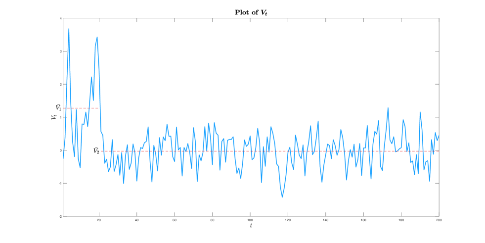
Figure 1: Plot of $V_{t}$ for model M1. The sample size is $T=200.$ $T_{1}^{0}=20$. Also reported in red dashed lines are the sample averages in the two regimes with $\overline{V}_{1}=1.27$ and $\overline{V}_{2}=-0.03$.

We begin with a simple model involving a zero-mean SLS process with changes in persistence. The combination of nonstationarity and serial dependence generates long memory effects because $\widehat{d}^{*}>0$. We specify $\left\{V_{t}\right\}$ as a SLS process given by a two-regimes zero-mean time-varying AR(1), labeled model M1. That is, $V_{t}=0.9V_{t-1}+u_{t}$, $u_{t}\sim\mathrm{i.i.d.}\,\mathscr{N}\left(0,\,1\right)$ for $t=1,\ldots,\,T_{1}^{0}$ with $T_{1}^{0}=T\lambda_{1}^{0}$, and $V_{t}=\rho\left(t/T\right)V_{t-1}+u_{t}$, $\rho\left(t/T\right)=0.3\left(\cos\left(1.5-\cos\left(t/T\right)\right)\right)$, $u_{t}\sim\mathscr{\mathrm{i.i.d.}\,\mathscr{N}}\left(0,\,0.5\right)$ for $t=T_{1}^{0}+1,\ldots,\,T$. Note that $\rho\left(\cdot\right)$ varies between 0.172 and 0.263. We set $\lambda_{1}^{0}=0.1$ and $T=200.$ A plot of $\left\{V_{t}\right\}$ is reported in Figure 1. Note that $\mathbb{E}\left(V_{t}\right)=0$ for all $t$ and so $d^{*}=d_{\mathrm{Sta}}^{*}=0$. However, if we replace $\overline{\mu}_{1}$ and $\overline{\mu}_{2}$ in $d^{*}$ by $\overline{V}_{1}$ and $\overline{V}_{2},$ respectively, where $\overline{V}_{1}=\left(T_{1}^{0}\right)^{-1}\sum_{t=1}^{T_{1}^{0}}V_{t}=1.27$ and $\overline{V}_{2}=\left(T-T_{1}^{0}\right)^{-1}\sum_{t=T_{1}^{0}+1}^{T}V_{t}=-0.03$, then the estimate $\widehat{d}^{*}$ of $d^{*}$ is different from zero and generates a finite-sample bias which can give rise to effects akin to long memory.

We first look at the behavior of the sample autocovariance $\widehat{\Gamma}\left(k\right)$. We compare it with the theoretical autocovariance $\Gamma_{T}\left(k\right)=T^{-1}\sum_{t=k+1}^{T}\mathbb{E}\left(V_{t}V_{t-k}\right)$. The latter is equal to $\Gamma_{T}\left(k\right)\thickapprox\lambda_{1}^{0}0.9^{k}/\left(1-0.81\right)+\int_{\lambda_{1}^{0}}^{1}c\left(u,\,k\right)du.$ We can compute $\Gamma_{T}\left(k\right)$ numerically using,

$$c\left(u,\,k\right) =\int_{-\pi}^{\pi}e^{ik\omega}f\left(u,\,\omega\right)d\omega=\int_{-\pi}^{\pi}e^{ik\omega}\frac{0.5}{2\pi}\left(1+\rho\left(u\right)^{2}-2\rho\left(u\right)\cos\left(\omega\right)\right)^{-1}d\omega.$$

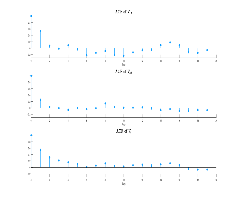
Figure 2: ACF of $V_{1,t}$ (top panel), ACF of $V_{2,t}$ (mid panel) and ACF of $V_{t}$ (bottom panel) for model M1.

Table 1 reports $\Gamma_{T}\left(k\right),$ $\widehat{\Gamma}\left(k\right)$, $\widehat{\Gamma}\left(k\right)-\widehat{d}^{*}$ and $\widehat{\Gamma}_{\mathrm{DK}}\left(k\right)$ for several values of $k$. Despite noisy autocovariance estimates, it is still possible to discern some patterns. For all $k$, $\widehat{\Gamma}\left(k\right)$ largely overestimates $\Gamma_{T}\left(k\right)$. This is consistent with Theorem 3.1 which suggests that this is due to the bias $d^{*}>0$. This is also supported by the bias-corrected estimate $\widehat{\Gamma}\left(k\right)-\widehat{d}^{*}$ which is accurate in approximating $\Gamma_{T}\left(k\right).$ This is especially so for small $k.$ In general, Theorem 3.1 provides good approximations confirming that $\widehat{\Gamma}\left(k\right)$ suffers from low frequency contaminations. Theorem 3.3 suggests that this issue should not occur for $\widehat{\Gamma}_{\mathrm{DK}}\left(k\right)$. In fact, $\widehat{\Gamma}_{\mathrm{DK}}\left(k\right)$ is more accurate than $\widehat{\Gamma}\left(k\right)$ (except for $k=0$). For $k\geq 20$ the form of $\Gamma_{T}\left(k\right)$ is different, because $T_{1}^{0}=20$, and is simply given by the autocovariance of $V_{t}$ for $t\geq 21$ (i.e., the second regime). Thus, $\Gamma_{T}\left(k\right)$$\thickapprox 0$ for $k\geq 20$ whereas $\widehat{\Gamma}\left(k\right)$ is often small but positive. In contrast, $\widehat{\Gamma}_{\mathrm{DK}}\left(k\right)\thickapprox 0$ for $k\geq 20$ thereby confirming that $\widehat{\Gamma}_{\mathrm{DK}}\left(k\right)$ does not suffer from low frequency contamination. These results are confirmed in Figure 2 which plots the autocorrelation function (ACF) of $V_{1,t}=V_{t}$ ($t=1,\ldots,\,20$), $V_{2,t}=V_{t}$ ($t=21,\ldots,\,200$) and $V_{t}$ ($t=1,\ldots,\,200$). Although the ACF of $V_{t}$ should be a weighted average of the ACF of $V_{1,t}$ and of $V_{2,t},$ the ACF of $V_{t}$ in the bottom panel shows much higher persistence than either ACF in the top $(V_{1,t})$ and mid $(V_{2,t})$ panels. This is odd since $V_{1,t}$ is a highly persistent series. Further, it shows that the dependence is essentially always positive. This is also odd. These features are consistent with our theory which suggests that nonstationarity makes $V_{t}$ appear more persistent and that the bias is positive. Other examples with similar features involve $V_{t}$ given by the least-squares regression residuals under mild forms of misspecification that do not undermine the conditions for consistency of the least-squares estimator, e.g., exclusion of a relevant regressor uncorrelated with the included reggressors, or inclusion of an irrelevant regressor. Another example involves $V_{t}$ obtained after applying some de-trending techniques where the fitted model is not correctly specified (e.g., the data follow a nonlinear trend but one removes a linear trend). A final example is the case of outliers because they influence the mean of $V_{t}$ and therefore $d^{*}$.

What is especially relevant is whether this evidence of long memory feature has any consequence for HAR inference. We obtain the empirical size and power for a $t$-test on the intercept normalized by several LRV estimators for the model $y_{t}=\delta+V_{t}$ with $\delta=0$ under the null and $\delta>0$ under the alternative hypothesis. In addition to M1, we consider other models: M2 involves a locally stationary process $V_{t}=\rho\left(t/T\right)V_{t-1}+u_{t}$, $\rho\left(t/T\right)=0.7(\cos\left(1.5t/T\right))$, $u_{t}\sim\mathscr{\mathrm{i.i.d.}\,\mathscr{N}}\left(0,\,0.5\right)$; M3 is the same as M2 with outliers $V_{t}\sim\mathrm{Uniform}\left(\underline{c},\,10\underline{c}\right)$ for $t=T/4,\,T/2,\,3T/4$ where $\underline{c}=-1/(\sqrt{2}\mathrm{erfc^{-1}\left(3/2\right))}\mathrm{med}\left(\left|V-\mathrm{med}\left(V\right)\right|\right)$ where $\mathrm{erfc}^{-1}$ is the inverse complementary error function, $\mathrm{med}\left(\cdot\right)$ is the median and $V=\left(V_{t}\right)_{t=1}^{T}$; M4 involves a locally stationary model with periods of strong persistence where $V_{t}=\rho\left(t/T\right)V_{t-1}+u_{t}$, $\rho\left(t/T\right)=0.95(\cos\left(1.5t/T\right))$, $u_{t}\sim\mathscr{\mathrm{i.i.d.}\,\mathscr{N}}\left(0,\,0.4\right)$. $\rho\left(\cdot\right)$ varies between 0.7 and 0.05 in M2-M3 and between 0.95 and 0.07 in M4.

We consider the DK-HAC estimators with and without prewhitening ($\widehat{J}_{\mathrm{DK},T}$, $\widehat{J}_{\mathrm{DK,pw},\mathrm{SLS},T}$, $\widehat{J}_{\mathrm{DK,pw},\mathrm{SLS},\mu,T}$) of Casini (2021c) and Casini and Perron (2021d), respectively; Andrews’ (1991) HAC estimator with and without the prewhitening procedure of Andrews and Monahan (1992); Newey and West’s (1987) HAC estimator with the usual rule to select the number of lags (i.e., $b_{1,T}=1/(0.75T^{1/3})$; Newey-West with the fixed-$b$ method of Kiefer et al. (2000) (labeled KVB); and the Empirical Weighted Cosine (EWC) of Lazarus et al. (2018). For the DK-HAC estimators we use the data-dependent methods for the bandwidths, kernels and choice of $n_{T}$ as proposed in Casini (2021c) and Casini and Perron (2021d), which are optimal under mean-squared error (MSE). Let $\widehat{V}_{t}$ denote the least-squares residual based on $\widehat{\delta}$ where the latter is the least-squares estimate of $\delta$. We set $\widehat{b}_{1,T}=0.6828(\widehat{\phi}\left(2\right)T\widehat{\overline{b}}_{2,T})^{-1/5}$ where

$$\widehat{\phi}\left(2\right) =\left(18\left(\frac{n_{T}}{T}\sum_{j=0}^{\left\lfloor T/n_{3,T}\right\rfloor-1}\frac{\left(\widehat{\sigma}\left(\left(jn_{T}+1\right)/T\right)\widehat{a}_{1}\left(\left(jn_{T}+1\right)/T\right)\right)^{2}}{\left(1-\widehat{a}_{1}\left(\left(jn_{T}+1\right)/T\right)\right)^{4}}\right)^{2}\right)/$$

$$\quad\left(\frac{n_{T}}{T}\sum_{j=0}^{\left\lfloor T/n_{3,T}\right\rfloor-1}\frac{\left(\widehat{\sigma}\left(\left(jn_{T}+1\right)/T\right)\right)^{2}}{\left(1-\widehat{a}_{1}\left(\left(jn_{T}+1\right)/T\right)\right)^{2}}\right)^{2},$$

with $\widehat{a}_{1}\left(u\right)=\frac{\sum_{j=t-n_{T}+1}^{t}\widehat{V}_{j}\widehat{V}_{j-1}}{\sum_{j=t-n_{T}+1}^{t}(\widehat{V}_{j-1})^{2}}$ and $\widehat{\sigma}\left(u\right)=(\sum_{j=t-n_{T}+1}^{t}(\widehat{V}_{j}-\widehat{a}_{1}\left(u\right)\widehat{V}_{j-1})^{2})^{1/2}$ and $\widehat{\overline{b}}_{2,T}=\left(n_{T}/T\right)\sum_{r=1}^{\left\lfloor T/n_{T}\right\rfloor-1}$ $\widehat{b}_{2,T}\left(rn_{T}/T\right)$, $\widehat{b}_{2,T}\left(u\right)=1.6786(\widehat{D}_{1}\left(u\right)){}^{-1/5}(\widehat{D}_{2}\left(u\right))^{1/5}T^{-1/5}$ where $\widehat{D}_{2}\left(u\right)\triangleq 2\sum_{l=-\left\lfloor T^{4/25}\right\rfloor}^{\left\lfloor T^{4/25}\right\rfloor}\widehat{c}_{\mathrm{DK,}T}\left(u,\,l\right)^{2}$ and

$$\widehat{D}_{1}\left(u\right) \triangleq(\left[S_{\omega}\right]^{-1}\sum_{s\in S_{\omega}}[3\pi^{-1}(1+0.8(\cos 1.5+\cos 4\pi u)\exp(-i\omega_{s}))^{-4}(0.8(-4\pi\sin(4\pi u)))\exp(-i\omega_{s})$$

$$\quad-\pi^{-1}\left|1+0.8(\cos 1.5+\cos 4\pi u)\exp(-i\omega_{s})\right|^{-3}(0.8(-16\pi^{2}\cos(4\pi u)))\exp(-i\omega_{s})])^{2},$$

with $\left[S_{\omega}\right]$ being the cardinality of $S_{\omega}$ and $\omega_{s+1}>\omega_{s}$, $\omega_{1}=-\pi,\,\omega_{\left[S_{\omega}\right]}=\pi.$ We set $n_{T}=T^{0.6}$, $S_{\omega}=\{-\pi,\,-3,\,-2,\,-1,\,0,\,1,\,2,\,3,\,\pi\}.$ $K_{1}\left(\cdot\right)$ is the QS kernel and $K_{2}\left(x\right)=6x\left(1-x\right)$ for $x\in\left[0,\,1\right].$

Table 2-5 report the results. The $t$-test normalized by Newey and West’s (1987) and Andrews’ (1991) prewhitened HAC estimators are excessively oversized. Andrews’ (1991) HAC-based test is slightly undersized while KVB’s fixed-$b$ and EWC-based tests are severely undersized. These outcomes arise from nonstationarity and are consistent with our theoretical analysis of $\widehat{\Gamma}\left(k\right)$. Since $\widehat{\Gamma}\left(k\right)>0$ for many large lags $k$, the KVB’s fixed-$b$ and EWC’s estimators that include many lags are inflated and reduce the magnitude of the test statistic even under the null hypotheses. The fact that KVB’s fixed-$b$ and EWC-based tests have larger size distortions than other tests is consistent with the results in Section 4 which suggest that they have a larger ERP. For the $t$-test on the intercept, $\widehat{J}_{\mathrm{DK},T}$ can lead to tests that are oversized when there is strong dependence, as shown in Table 2. However, the prewhitened DK-HAC estimators $\widehat{J}_{\mathrm{DK,pw},\mathrm{SLS},T}$ and $\widehat{J}_{\mathrm{DK,pw},\mathrm{SLS},\mu,T}$ lead to tests that show very accurate rejection rates. Overall, inspection of the size properties suggests that the DK-HAC-based tests do not suffer from low frequency contamination which, in contrast, affects the tests based on LRV estimators that rely on the full sample estimates $\widehat{\Gamma}\left(k\right)$ or equivalently on $I_{T}\left(\omega\right)$ (e.g., the EWC). The same issue also affects the power properties of the tests. The KVB’s fixed-$b$ and EWC-based estimators suffer from relatively large power losses. The power of tests normalized by Newey and West’s (1987) and Andrews’ (1991) prewhitened HAC are not comparable because they are significantly oversized. The DK-HAC-based tests have the best power, the second best being Andrews’ (1991) HAC-based test.

Turning to M2, Table 3 shows even larger size distortions and power losses for KVB’s fixed-$b$ and EWC-based tests. All the DK-HAC-based tests display accurate size control and good power. Newey and West’s (1987) and Andrews’ (1991) prewhitened HAC-based tests are again excessively oversized. Andrews’ (1991) HAC-based test sacrifices some power relative to the DK-HAC-based test even though the margin is not high. For model M3-M4, Table 4-5 show that Andrews’ (1991) HAC-based test also suffers from strong size distortions and power losses, thus sharing the same issues as KVB’s fixed-$b$ and EWC-based tests. In model M4, even Newey and West’s (1987) and Andrews’ (1991) prewhitened HAC-based tests are undersized and have relatively low power. The DK-HAC-based tests perform best both in terms of size and power. Table 2-5 suggest that the low frequency contamination can equally arise from different forms of nonstationarity. Overall, the evidence for quite substantial underejection and power losses in model M1-M4 for the existing HAR tests is consistent with our theoretical results. These represent situations where the contamination occurs as a small-sample problem and the ERP is larger for fixed-$b$-based HAR tests. In the next section, we show that when the contamination holds asymptotically then the size distortions and power problems can be even more severe.

5.3 General Low Frequency Contamination

We now discuss HAR inference tests for which the low frequency contamination results of Section 3 hold even asymptotically. This means that $d^{*}>0$ for all $T$ and as $T\rightarrow\infty$. This comprises the class of HAR tests that admit a nonstationary alternative hypotheses. This class is very large and include most HAR tests as discussed in the Introduction. Here we consider the Diebold-Mariano test for the sake of illustration and remark that similar issues apply to other HAR tests.

The Diebold-Mariano test statistic is defined as $t_{\mathrm{DM}}\triangleq T_{n}^{1/2}\overline{d}_{L}/\sqrt{\widehat{J}_{d_{L},T}}$, where $\overline{d}_{L}$ is the average of the loss differentials between two competing forecast models, $\widehat{J}_{d_{L},T}$ is an estimate of the LRV of the the loss differential series and $T_{n}$ is the number of observations in the out-of-sample. We use the quadratic loss. We consider an out-of-sample forecasting exercise with a fixed forecasting scheme where, given a sample of $T$ observations, $0.5T$ observations are used for the in-sample and the remaining half is used for prediction [see Perron and Yamamoto (2021) for recommendations on using a fixed scheme in the presence of breaks]. The DGP under the null hypotheses is given by $y_{t}=1+\beta_{0}x_{t-1}^{(0)}+e_{t}$ where $x_{t-1}^{(0)}\sim\mathrm{i.i.d.}\,\mathscr{N}\left(1,\,1\right)$, $e_{t}=0.3e_{t-1}+u_{t}$ with $u_{t}\sim\mathrm{i.i.d.\,}\mathscr{N}\left(0,\,1\right)$, and we set $\beta_{0}=1$ and $T=400.$ The two competing models both involve an intercept but differ on the predictor used in place of $x_{t}^{(0)}$. The first forecast model uses $x_{t}^{(1)}$ while the second uses $x_{t}^{(2)}$ where $x_{t}^{(1)}$ and $x_{t}^{(2)}$ are independent $\mathrm{i.i.d.}\,\mathscr{N}\left(1,\,1\right)$ sequences, both independent from $x_{t}^{(0)}$. Each forecast model generates a sequence of $\tau\left(=1\right)$-step ahead out-of-sample losses $L_{t}^{(j)}$ $\left(j=1,\,2\right)$ for $t=T/2+1,\ldots,\,T-\tau.$ Then $d_{t}\triangleq L_{t}^{(2)}-L_{t}^{(1)}$ denotes the loss differential at time $t$. The Diebold-Mariano test rejects the null hypotheses of equal predictive ability when $\overline{d}_{L}$ is sufficiently far from zero. Under the alternative hypothesis, the two competing forecast models are as follows: the first uses $x_{t}^{(1)}=x_{t}^{(0)}+u_{X_{1},t}$ where $u_{X_{1},t}\sim\mathrm{i.i.d.\,}\mathscr{N}\left(0,\,1\right)$ while the second uses $x_{t}^{(2)}=x_{t}^{(0)}+0.2z_{t}+2u_{X_{2},t}$ for $t\in\left[1,\ldots,\,3T/4-1,\,3T/4+21,\ldots T\right]$ and $x_{t}^{(2)}=\delta\left(t/T\right)+0.2z_{t}+2u_{X_{2},t}$ for $t=3T/4,\ldots,\,3T/4+20$ with $u_{X_{2},t}\sim\mathrm{i.i.d.\,}\mathscr{N}\left(0,\,1\right)$, where $z_{t}$ has the same distribution as $x_{t}^{(0)}.$

We consider four specifications for $\delta\left(\cdot\right).$ In the first $x_{t}^{(2)}$ is subject to an abrupt break in the mean $\delta\left(t/T\right)=\delta>0$; in the second $x_{t}^{(2)}$ is locally stationary with time-varying mean $\delta\left(t/T\right)=\delta\left(\sin\left(t/T-3/4\right)\right)$; in the third specification $x_{t}^{(2)}=x_{t}^{(0)}+0.2z_{t}+2u_{X_{2},t}$ for $t\in[1,\ldots,\,T/2-30,\,T/2$ $+21,\ldots T]$ and $x_{t}^{(2)}=\delta\left(t/T\right)+0.2z_{t}+2u_{X_{2},t}$ for $t=T/2-30,\ldots,\,T/2+20$ with $\delta\left(t/T\right)=\delta(\sin(t/T-1/2$ $-30/T))$; in the fourth $x_{t}^{(2)}$ is the same as in the second with in addition two outliers $x_{t}^{(2)}\sim\mathrm{Uniform}\left(\left|\underline{c}\right|,\,5\left|\underline{c}\right|\right)$ for $t=6T/10,\,8T/10$ where $\underline{c}=-1/(\sqrt{2}\mathrm{erfc^{-1}\left(3/2\right))}\mathrm{med}(|x^{(2)}-\mathrm{med}$ $(x^{(2)})|)$ where $x^{(2)}=(x_{t}^{(2)})_{t=1}^{T}$. That is, in the second model $x_{t}^{(2)}$ is locally stationary only in the out-of-sample, in the third it is locally stationary in both the in-sample and out-of sample and in the fourth model $x_{t}^{(2)}$ has two outliers in the out-of-sample. The location of the outliers is irrelevant for the results; they can also occur in the in-sample.

Table 6 reports the size and the power of the various tests for all models. We begin with the case $\delta\left(t/T\right)=\delta>0$ (top panel). The size of the test using the DK-HAC estimators is accurate while the test using other LRV estimators are oversized with the exception of the KVB’s fixed-$b$ method for which the rejection rate is equal to zero. The HAR tests using existing LRV estimators have lower power relative to that obtained with the DK-HAC estimators for small values of $\delta$. When $\delta$ increases the tests standardized by the HAC estimators of Andrews (1991) and Newey and West (1987), and by the KVB’s fixed-$b$ and EWC LRV estimators display non-monotonic power gradually converging to zero as the alternative gets further away from the null value. In contrast, when using the DK-HAC estimators the test has monotonic power that reaches and maintains unit power. The results for the other models are even stronger. In general, except when using the DK-HAC estimators, all tests display serious power problems. Thus, either form of nonstationarity or outliers leads to similar implications, consistent with our theoretical results.

In order to further assess the theoretical results from Section 3, Figure 3 reports the plots of $d_{t}$, its sample autocovariances and its periodogram, for $\delta=1$. Figure S.1-S.2 in the supplement report the corresponding plots for $\delta=2,\,5$, respectively. We only consider the case $\delta_{t}=\delta>0$. The other cases lead to the same conclusions. For $\delta=1$, Figure 3 (mid panel) shows that $\widehat{\Gamma}\left(k\right)$ decays slowly. As $\delta$ increases, Figure S.1 and S.2 (mid panels), $\widehat{\Gamma}\left(k\right)$ decays even more slowly at a rate far from the typical exponential decay of short memory processes. This suggests evidence of long memory. However, the data are short memory with small temporal dependence. What is generating the spurious long memory effect is the nonstationarity present under the alternative hypotheses. This is visible in the top panels which present plots of $d_{t}$ for the first specification. The shift in the mean of $d_{t}$ for $t=3T/4,\ldots,\,3T/4+20$ is responsible for the long memory effect. This corresponds to the second term of (3.3) in Theorem 3.1. The overall behavior of the sample autocovariance is as predicted by Theorem 3.1. For small lags, $\widehat{\Gamma}\left(k\right)$ shows a power-like decay and it is positive. As $k$ increases to medium lags, the autocovariances turn negative because the sum of all sample autocovariances has to be equal to zero [cf. Percival (1992)]. Next, we move to the bottom panels which plot the periodogram of $\{d_{t}\}$. It is unbounded at frequencies close to $\omega=0$ as predicted by Theorem 3.2 and as would occur if long memory was present. It also explains why the Diebold-Mariano test normalized by Newey-West’s, Andrews’, KVB’s fixed-$b$ and EWC’s LRV estimators have serious power problems. These LRV estimators are inflated and consequently the tests lose power. The figures show that as we raise $\delta$ the more severe these issues and the power losses so that the power eventually reaches zero. This is consistent with our theory since $d^{*}$ is increasing in $\delta$ (cf. $d^{*}\thickapprox 0.1\cdot 0.9\delta^{2}$).

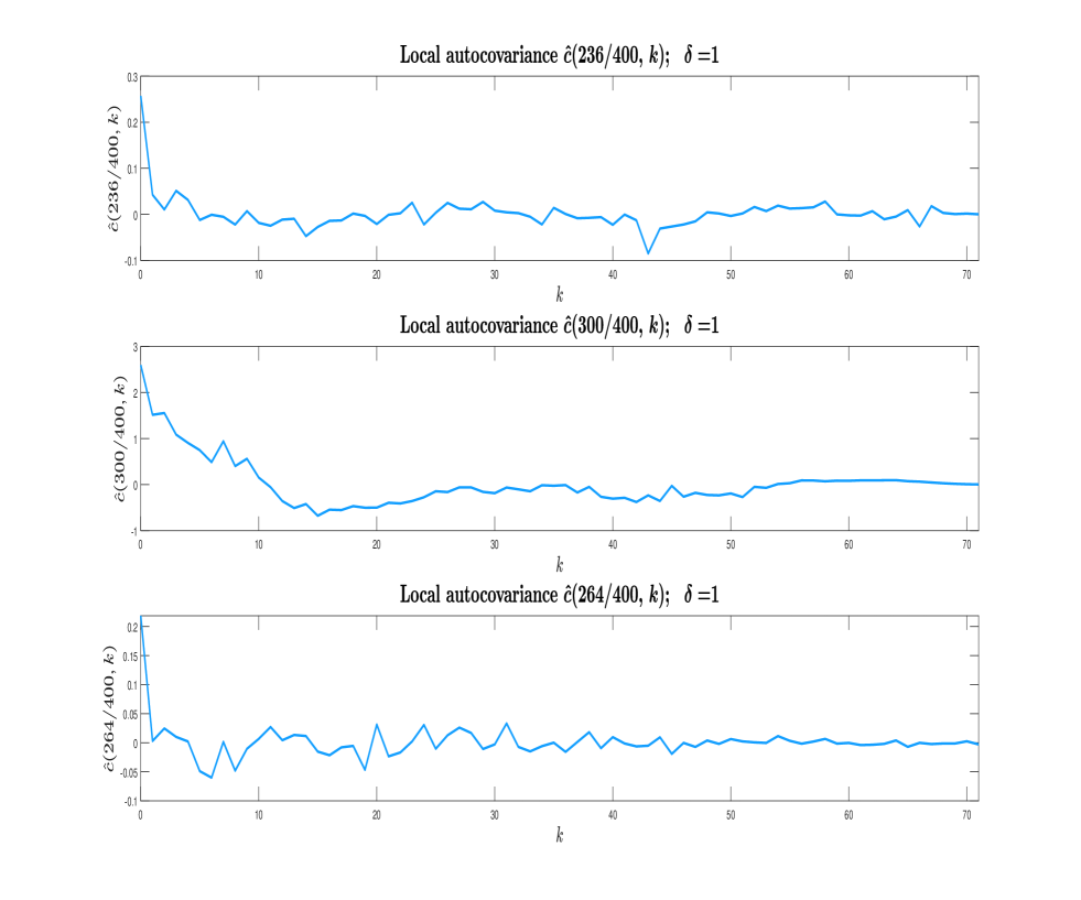
Figure 4: The figure plots $\widehat{c}_{T}\left(u,\,k\right)$ for $u=236/400,\,\lambda_{1}^{0},\,264/400$ in the top, mid and bottom panel, respectively. In all panels $\delta=1.$

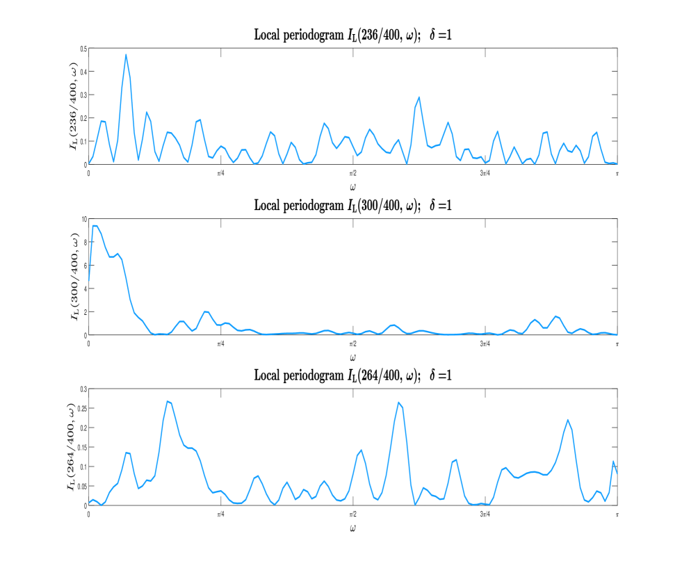
Figure 5: The figure plots $I_{\mathrm{L}}\left(u,\,\omega\right)$ for $u=236/400,\,\lambda_{1}^{0},\,264/400$ in the top, mid and bottom panel, respectively. In all panels $\delta=1.$

We now verify the results about the local sample autocovariance $\widehat{c}_{T}\left(u,\,k\right)$ and the local periodogram from Theorem 3.3-3.4. We set $n_{2,T}=T^{0.6}=36$ following the MSE criterion of Casini (2021c). We consider (i) $u=236/T$, (ii-a) $u=T_{1}^{0}/T=3/4$ and (ii-b) $u=264/T$. Note that cases (i)-(ii-b) correspond to parts (i)-(ii-b) in Theorem 3.3-3.4. We consider $\delta=1,\,2$ and $5$. According to Thereon 3.3-3.4, we should expect long memory features only for case (ii-a). Figure 4-5 and S.3-S.6 in the supplement confirm this. The results pertaining to case (ii-a) are plotted in the middle panels. Figures 4, S.3 and S.5 show that the local autocovariance displays slow decay similar to the pattern discussed above for $\widehat{\Gamma}\left(k\right)$ and that this problem becomes more severe as $\delta$ increases. Such long memory features also appear for $I_{\mathrm{L}}\left(3/4,\,\omega\right)$. The middle panels in Figure 5, S.4 and S.6 show that the local periodogram at $u=3/4$ and at a frequency close to $\omega=0$ are extremely large. The latter result is consistent with Theorem 3.4-(ii-a) which suggests that $I_{\mathrm{L,}T}\left(3/4,\,\omega\right)\rightarrow\infty$ as $\omega\rightarrow 0$. For case (i) and (ii-b) both figures show that the local autocovariance and the local periodogram do not display long memory features. Indeed, they have forms similar to those of a short memory process, a result consistent with Theorem 3.3-3.4 also for cases (i) and (ii-b).

It is interesting to explain why HAR inference based on the DK-HAC estimators does not suffer from the low frequency contamination even if case (ii-a) occurs. The DK-HAC estimator computes an average of the local spectral density over time blocks. If one of these blocks contains a discontinuity in the spectrum, then as in case (ii-a) some bias would arise for the local spectral density estimate corresponding to that block. However, by virtue of the time-averaging over blocks that bias becomes negligible. Hence, nonparametric smoothing over time asymptotically cancels the bias, so that inference based on the DK-HAC estimators is robust to nonstationarity.

5.4 Theoretical Results about the Power

We present theoretical results about the power of $t_{\mathrm{DM}}$ for the case of general low frequency contamination discussed in Section 5.3. In particular, we focus on specification (1) (i.e., $\delta>0$). The same intuition and qualitative theoretical results apply to the other specifications of $\delta\left(\cdot\right)$.

Let $t_{\mathrm{DM},i}=T_{n}^{1/2}\overline{d}_{L}/\sqrt{\widehat{J}_{d_{L},i,T}}$ denote the DM test statistic where $i=\mathrm{DK},\,\mathrm{pwDK},\,\mathrm{KVB},\,\mathrm{EWC},$ $\mathrm{A91},\,\mathrm{pwA}91$, $\mathrm{NW87}$ and $\mathrm{pwNW87}$ with $\widehat{J}_{\mathrm{A91},T}$ and $\widehat{J}_{\mathrm{NW87},T}$ being $\widehat{J}_{\mathrm{HAC},T}$ using the quadratic spectral and Bartlett kernel, respectively. Define the power of $t_{\mathrm{DM},i}$ as $\mathbb{P}_{\delta}(|t_{\mathrm{DM},i}|>z_{\alpha})$ where $z_{\alpha}$ is the two-sided standard normal critical value and $\alpha\in\left(0,\,1\right)$ is the significance level. To avoid repetitions we present the results only for $i=\mathrm{DK},\,\mathrm{KVB}$ and $\mathrm{NW87}$. The results concerning the prewhitening DK-HAC estimator are the same as those corresponding to the DK-HAC estimator while the results concerning the EWC estimator are the same as those corresponding to the KVB’s fixed-$b$ estimator. The results pertaining to Andrews’ (1991) HAC estimator (with and without prewhitening) are the same as those corresponding to Newey and West’s (1987) estimator. Let $n_{\delta}$ denote the length of the regime in which $x_{t}^{(2)}$ exhibits a shift $\delta$ in the mean and let $T^{*}\left(n_{\delta}\right)$ be an integer function of $n_{\delta}$ with $T^{*}\left(n_{\delta}\right)>0$ that may depend on $T$.

Theorem 5.1.

Let $\left\{d_{t}\right\}_{t=1}^{T_{n}}$ be a SLS process satisfying Assumption 2.1-(i-iv) and 2.2. Let Assumption 4.3-4.4 hold. Then, we have:

(i) Under Assumption 4.6, $\mathbb{P}_{\delta}(|t_{\mathrm{DM},\mathrm{NW87}}|>z_{\alpha})\rightarrow 0$. If Assumption 4.6 is replaced by Assumption 4.7 with $q=1/3$, then $|t_{\mathrm{DM},\mathrm{NW87}}|=7.06O_{\mathbb{P}}(T_{n}^{-1/6})$ and $\mathbb{P}_{\delta}(|t_{\mathrm{DM},\mathrm{NW87}}|>z_{\alpha})$$\rightarrow 0.$

(ii) If $b_{1,T}=T^{-1}$, then $|t_{\mathrm{DM},\mathrm{KVB}}|=7.06O_{\mathbb{P}}(T_{n}^{-1/2})$ and $\mathbb{P}_{\delta}(|t_{\mathrm{DM},\mathrm{KVB}}|>z_{\alpha})$$\rightarrow 0.$

(iii) Under Assumption 4.8, $|t_{\mathrm{DM},\mathrm{DK}}|=\delta^{2}O_{\mathbb{P}}(T^{*}(n_{\delta}))$ and $\mathbb{P}_{\delta}(|t_{\mathrm{DM},\mathrm{DK}}|>z_{\alpha})$$\rightarrow 1,$ where $\{T^{*}(n_{\delta})\}$ is such that $T^{*}\left(n_{\delta}\right)\rightarrow\infty$ as $T\rightarrow\infty$ with $T^{*}\left(n_{\delta}\right)=T_{n}^{\zeta}$ and $\zeta\in(0,\,1/2]$.

Note that Assumption 4.7 with $q=1/3$ refers to the MSE-optimal bandwidth for the Newey and West’s (1987) estimator. The sequence $\{T^{*}(n_{\delta})\}$ in part (iii) depends on the form of the alternative hypothesis. Theorem 5.1 implies that when the classical HAC estimators or the fixed-$b$ LRV estimators are used, the DM test is not consistent and its power converges to zero. The theorem also implies that the power functions corresponding to tests based on HAC estimators lie above the power functions corresponding to those based on fixed-$b$/EWC LRV estimators. This follows from $|t_{\mathrm{DM},\mathrm{KVB}}|\ll|t_{\mathrm{DM},\mathrm{NW87}}|.$ Another interesting feature is that $|t_{\mathrm{DM},\mathrm{NW87}}|$ and $|t_{\mathrm{DM},\mathrm{KVB}}|$ do not increase in magnitude with $\delta$ because $\delta$ appears in both the numerator and denominator [$\delta$ enters the denominator through the low frequency contamination term $d^{*}$ that accounts for the bias in the HAC and fixed-$b$ estimators [cf. Theorem 3.1]]. Part (iii) of the theorem suggests that these issues do not occur when DK-HAC estimator is used since the test is consistent and its power increases with $\delta$ and with the sample size as it should be. These results match the empirical results in Table 6 discussed above, thereby confirming the relevance of Theorem 5.1.

5.5 Discussion

In summary, the sample autocovariance and the periodogram are sensitive to nonstationarity in that they may display characteristics typical of long memory when the data are short memory subject to low frequency contamination. In some cases these issues only imply a small-sample problem [cf. Section 5.2]. In others, they have an effect even asymptotically. In either case, the theory in Section 3 provides useful guidance about the properties of the sample autocovariance and the periodogram in finite-samples. It also provides accurate approximations for misspecified models or models with outliers. Since LRV estimates are direct inputs for inference in the context of autocorrelated data, our theory offers new insights for the properties of HAR inference tests. The use of HAC standard errors has become the standard practice, and recent theoretical developments in HAR inference advocated the use of fixed-$b$ or long bandwidth LRV estimators on the basis that they offer better size control when there is strong dependence in the data. Our results suggest that care is needed before applying such methods because they are highly sensitive to effects akin to long memory arising from nonstationarity. The concern is then that the use of long bandwidths leads to overestimation of the true LRV due to low frequency contamination. Consequently, HAR tests can dramatically lose power, a problem that occurs also for the classical HAC estimators, though to a lesser extent since they use a smaller number of sample autocovariances.

Our theory also suggests a solution to this problem. This entails the use of nonparametric smoothing over time which avoids combining observations that belong to different regimes. This accounts for nonstationarity and prevents spurious long memory effects.

6 Conclusions

Economic time series are highly nonstationary and models might be misspecified. If nonstationary is not accounted for properly, parameter estimates and, in particular, asymptotic LRV estimates can be largely biased. We establish results on the low frequency contamination induced by nonstationarity and misspecification for the sample autocovariance and the periodogram under general conditions. These estimates can exhibit features akin to long memory when the data are nonstationary short memory. We distinguish cases where this contamination only implies a small-sample problem and cases where the problem remains asymptotically. We show, using theoretical arguments, that nonparametric smoothing is robust. Since the autocovariances and the periodogram are basic elements for HAR inference, our results provide insights on the important debate between consistent versus inconsistent LRV estimation. Our results show that existing LRV estimators tend to be inflated when the data are nonstationarity. This results in HAR tests that can be undersized and exhibit dramatic power losses or even no power. Long bandwidths/fixed-$b$ HAR tests suffer more from low frequency contamination relative to HAR tests based on HAC estimators, whereas the DK-HAC estimators do not suffer from this problem.

Supplemental Materials

supplement for online publication [cf. Casini et al. (2021)] introduces the notion of long memory segmented locally stationary processes and contains the proofs of the results in the paper and additional figures.

Appendix A Appendix

Figure 3: a) top panel: plot of $\{d_{t}\};$ b) mid-panel: plot of the sample autocovariances $\widehat{\Gamma}\left(k\right)$ of $\{d_{t}\}$; c) bottom panel: plot the periodogram $I\left(\omega\right)$ of $\{d_{t}\}$. In all panels $\delta=1.$

Table 1: Comparison between the theoretical autocovariance and the sample estimates

	$\Gamma_{T}\left(k\right)$	$\widehat{\Gamma}\left(k\right)$	$\widehat{\Gamma}\left(k\right)-\widehat{d}^{*}$	$\widehat{\Gamma}_{\mathrm{DK}}\left(k\right)$
$k=0$	0.37	0.54	0.37	0.63
$k=1$	0.13	0.29	0.13	0.25
$k=2$	0.01	0.16	0.01	0.03
$k=5$	0.00	0.05	-0.03	0.00
$k=10$	-0.03	0.02	-0.07	0.00

The table reports the values of a) the theoretical autocovariance $\Gamma_{T}\left(k\right)$; b) the sample autocovariance $\widehat{\Gamma}\left(k\right)$; c) the corrected sample autocovariance $\widehat{\Gamma}\left(k\right)-\widehat{d}$; d) the double kernel sample autocovariance $\widehat{\Gamma}_{\mathrm{DK}}\left(k\right)$, for $k=0,\,1,\,2,\,5$ and 10, with the process $\left\{V_{t}\right\}$ as in model M1 with $T=200$.

Table 2: Empirical small-sample size and power of $t$-test for model M1

$\alpha=0.05,\,T=200$	$\delta=0$ (size)	$\delta=0.05$	$\delta=0.1$	$\delta=0.15$	$\delta=0.25$	$\delta=1$	$\delta=1.5$
$\widehat{J}_{\mathrm{DK,}T}$	0.068	0.189	0.286	0.460	0.661	0.992	1.000
$\widehat{J}_{\mathrm{DK,pw},\mathrm{SLS},T}$	0.045	0.085	0.199	0.332	0.612	0.976	1.000
$\widehat{J}_{\mathrm{DK,pw},\mathrm{SLS},\mu,T}$	0.046	0.090	0.202	0.333	0.613	0.977	1.000
Andrews (1991)	0.039	0.095	0.185	0.383	0.623	0.968	0.999
Andrews (1991), prewhite	0.115	0.168	0.304	0.447	0.650	0.988	0.999
Newey-West (1987)	0.209	0.272	0.398	0.516	0.689	0.997	1.000
Newey-West (1987), fixed-$b$ (KVB)	0.004	0.018	0.063	0.139	0.301	0.870	0.969
EWC	0.011	0.038	0.137	0.273	0.539	0.978	0.999

Table 3: Empirical small-sample size and power of the of $t$-test for model M2

$\alpha=0.05,\,T=200$	$\delta=0$ (size)	$\delta=0.15$	$\delta=0.2$	$\delta=0.25$	$\delta=0.3$	$\delta=0.5$
$\widehat{J}_{\mathrm{DK,}T}$	0.059	0.415	0.815	0.974	0.974	1.000
$\widehat{J}_{\mathrm{DK,pw},\mathrm{SLS},T}$	0.058	0.262	0.632	0.899	0.899	1.000
$\widehat{J}_{\mathrm{DK,pw},\mathrm{SLS},\mu,T}$	0.053	0.246	0.616	0.894	0.894	1.000
Andrews (1991)	0.064	0.228	0.564	0.892	0.830	1.000
Andrews (1991), prewhite	0.252	0.564	0.904	0.992	0.991	1.000
Newey-West (1987)	0.133	0.388	0.821	0.981	0.971	1.000
Newey-West (1987), fixed-$b$ (KVB)	0.000	0.077	0.018	0.356	0.356	0.971
EWC	0.004	0.045	0.255	0.632	0.637	1.000

Table 4: Empirical small-sample size and power of the of $t$-test for model M3

$\alpha=0.05,\,T=200$	$\delta=0$ (size)	$\delta=0.1$	$\delta=0.15$	$\delta=0.2$	$\delta=0.25$
$\widehat{J}_{\mathrm{DK,}T}$	0.086	0.552	0.930	0.992	1.000
$\widehat{J}_{\mathrm{DK,pw},\mathrm{SLS},T}$	0.065	0.436	0.887	0.971	1.000
$\widehat{J}_{\mathrm{DK,pw},\mathrm{SLS},\mu,T}$	0.063	0.415	0.875	0.981	1.000
Andrews (1991)	0.017	0.257	0.696	0.950	0996
Andrews (1991), prewhite	0.036	0.456	0.864	0.952	0.998
Newey-West (1987)	0.031	0.344	0.795	0.976	0.994
Newey-West (1987), fixed-$b$ (KVB)	0.000	0.084	0.245	0.442	0.627
EWC	0.000	0.051	0.299	0.699	0.937

Table 5: Empirical small-sample size and power of the of $t$-test for model M4

$\alpha=0.05,\,T=200$	$\delta=0$ (size)	$\delta=0.1$	$\delta=0.15$	$\delta=0.2$	$\delta=0.25$	$\delta=0.5$
$\widehat{J}_{\mathrm{DK,}T}$	0.067	0.558	0.748	0.870	0.945	1.000
$\widehat{J}_{\mathrm{DK,pw},\mathrm{SLS},T}$	0.065	0.301	0.495	0.618	0.736	1.000
$\widehat{J}_{\mathrm{DK,pw},\mathrm{SLS},\mu,T}$	0.037	0.351	0.508	0.656	0.766	1.000
Andrews (1991)	0.016	0.253	0.448	0.564	0.675	0.999
Andrews (1991), prewhite	0.456	0.804	0.916	0.904	0.992	1.000
Newey-West (1987)	0.346	0.954	0.981	0.821	0.981	1.000
Newey-West (1987), fixed-$b$ (KVB)	0.000	0.000	0.000	0.005	0.015	0.333
EWC	0.024	0.240	0.486	0.596	0.681	0.999

Table 6: Empirical small-sample size and power of the DM (1995) test

		(1) $\delta>0$
$\alpha=0.05,\,T=200$	size	$\delta=0.2$	$\delta=0.5$	$\delta=2$	$\delta=5$	$\delta=10$
$\widehat{J}_{\mathrm{DK,}T}$	0.033	0.312	0.551	0.997	1.000	1.000
$\widehat{J}_{\mathrm{DK,pw},\mathrm{SLS},T}$	0.042	0.322	0.563	0.999	1.000	1.000
$\widehat{J}_{\mathrm{DK,pw},\mathrm{SLS},\mu,T}$	0.046	0.348	0.573	0.998	1.000	1.000
Andrews (1991)	0.085	0.254	0.305	0.114	0.000	0.000
Andrews (1991), prewhite	0.085	0.246	0.293	0.401	0.045	0.000
Newey-West (1987)	0.083	0.246	0.299	0.612	0.817	0.782
Newey-West (1987), fixed-$b$ (KVB)	0.002	0.212	0.185	0.000	0.000	0.000
EWC	0.083	0.252	0.268	0.045	0.000	0.000
		(2) $\delta\left(t/T\right)$ locally stationary
$\alpha=0.05,\,T=200$		$\delta=0.2$	$\delta=0.5$	$\delta=2$	$\delta=5$	$\delta=10$
$\widehat{J}_{\mathrm{DK,}T}$		0.278	0.297	0.592	0.889	1.000
$\widehat{J}_{\mathrm{DK,pw},\mathrm{SLS},T}$		0.301	0.363	0.634	0969	1.000
$\widehat{J}_{\mathrm{DK,pw},\mathrm{SLS},\mu,T}$		0.327	0.368	0.642	0.969	1.000
Andrews (1991)		0.255	0.259	0.255	0.110	0.005
Andrews (1991), prewhite		0.249	0.243	0.268	0.188	0.031
Newey-West (1987)		0.281	0.282	0.313	0.268	0.078
Newey-West (1987), fixed-$b$ (KVB)		0.203	0.202	0.178	0.025	0.000
EWC		0.244	0.252	0.219	0.045	0.000
		(3) $\delta\left(t/T\right)$ locally stationary
$\alpha=0.05,\,T=200$		$\delta=0.2$	$\delta=1$	$\delta=2$	$\delta=5$	$\delta=10$
$\widehat{J}_{\mathrm{DK,}T}$		0.540	0.862	0.992	1.000	1.000
$\widehat{J}_{\mathrm{DK,pw},\mathrm{SLS},T}$		0.396	0.664	0.988	1.000	1.000
$\widehat{J}_{\mathrm{DK,pw},\mathrm{SLS},\mu,T}$		0.412	0.724	0.987	1.000	1.000
Andrews (1991)		0.328	0.234	0.235	0.241	0.777
Andrews (1991), prewhite		0.342	0.315	0.512	0.296	0.882
Newey-West (1987)		0.381	0.384	0.720	0.972	0.999
Newey-West (1987), fixed-$b$ (KVB)		0.100	0.032	0.000	0.002	0.040
EWC		0.312	0.152	0.142	0.296	0.852
		(4) case (2) with outliers
$\alpha=0.05$, $T=400$		$\delta=0.5$	$\delta=1$	$\delta=2$	$\delta=5$	$\delta=10$
$\widehat{J}_{\mathrm{DK,}T}$		0.694	0.733	0.822	0.981	1.000
$\widehat{J}_{\mathrm{DK,pw},\mathrm{SLS},T}$		0.724	0.777	0.846	0.982	1.000
$\widehat{J}_{\mathrm{DK,pw},\mathrm{SLS},\mu,T}$		0.727	0.771	0.847	0.981	1.000
Andrews (1991)		0.192	0.242	0.245	0.203	0.022
Andrews (1991), prewhite		0.182	0.233	0.243	0.288	0.114
Newey-West (1987)		0.222	0.271	0.245	0.345	0.225
Newey-West (1987), fixed-$b$ (KVB)		0.203	0.222	0.212	0.075	0.000
EWC		0.186	0.221	0.174	0.062	0.000

Supplement to “Theory of Low Frequency Contamination from Nonstationarity and Misspecication: Consequences for HAR Inference"

Alessandro Casini      Taosong Deng     Pierre Perron

University of Rome Tor Vergata     Hunan University       Boston University
March 9, 2024

Appendix S.A Long Memory Segmented Locally Stationary Processes

In this section we define long memory SLS processes. Define the backward difference operator $\Delta V_{t}=\Delta^{1}V_{t}=V_{t}-V_{t-1}$ and $\Delta^{l}V_{t}$ recursively. Long memory features can be expressed as a “pole” in the spectral density at frequency zero. That is, for a stationary process, long memory implies that $f\left(\omega\right)\thicksim\omega^{-2\vartheta}$ as $\omega\rightarrow 0$ where $\vartheta\in\left(0,\,1/2\right)$ is the long memory parameter. In what follows, $l$ is some non-negative integer.

Definition S.A.1.

A sequence of stochastic processes $\left\{V_{t,T}\right\}$ is called long memory segmented locally stationary with $m_{0}+1$ regimes, transfer function $A^{0}$ and trend $\mu_{\cdot}$ if there exists a representation

$$\Delta^{l}V_{t} =\mu_{j}\left(t/T\right)+\int_{-\pi}^{\pi}\exp\left(i\omega t\right)A_{j,t,T}^{0}\left(\omega\right)d\xi\left(\omega\right),\qquad\qquad\left(t=T_{j-1}^{0}+1,\ldots,\,T_{j}^{0}\right),$$ (S.1)

for $j=1,\ldots,\,m_{0}+1$, where by convention $T_{0}^{0}=0$ and $T_{m_{0}+1}^{0}=T$, (i) and (iii) of Definition 2.1 hold, and (ii) of Definition 2.1 is replaced by

(ii) There exists two constants $L_{2}>0$ and $D<1/2$ (which depend on $j$) and a piecewise continuous function $A:\,\left[0,\,1\right]\times\mathbb{R}\rightarrow\mathbb{C}$ such that, for each $j=1,\ldots,\,m_{0}+1$, there exists a $2\pi$-periodic function $A_{j}:\,(\lambda_{j-1}^{0},\,\lambda_{j}^{0}]\times\mathbb{R}\rightarrow\mathbb{C}$ with $A_{j}\left(u,\,-\omega\right)=\overline{A_{j}\left(u,\,\omega\right)}$,

$$A\left(u,\,\omega\right) =A_{j}\left(u,\,\omega\right)\,\mathrm{\,for\,}\,\lambda_{j-1}^{0}<u\leq\lambda_{j}^{0},$$ (S.2)

$$\sup_{1\leq j\leq m_{0}+1} \sup_{T_{j-1}^{0}<t\leq T_{j}^{0},\,\omega}\left|A_{j,t,T}^{0}\left(\omega\right)-A_{j}\left(t/T,\,\omega\right)\right|\leq L_{2}T^{-1}\left|\omega\right|^{-D},$$ (S.3)

and

$$\sup_{0\leq v\leq u\leq 1,\,u\neq\lambda_{j}^{0}\,\left(j=1,\ldots,\,m_{0}+1,\right),\,\omega}\left|A\left(u,\,\omega\right)-A\left(u^{\prime},\,\omega\right)\right| \leq L_{2}\left|u-u^{\prime}\right|\left|\omega\right|^{-D}.$$ (S.4)

The spectral density of $\{V_{t,T}\}$ is given by $f_{j}\left(u,\,\omega\right)=|1-\exp\left(-i\omega\right)|^{-2l}|A_{j}\left(u,\,\omega\right)|^{-2}$ for $j=1,\ldots,\,m_{0}+1$. We say that the process $\left\{V_{t,T}\right\}$ has local memory parameter $\vartheta\left(u\right)\in\left(-\infty,\,l+1/2\right)$ at time $u\in\left[0,\,1\right]$ if it satisfies (S.1)-(S.4), and its generalized spectral density $f_{j}\left(u,\,\omega\right)$ $(j=1,\ldots,$ $m_{0}+1)$ satisfies the following condition,

$$f_{j}\left(u,\,\omega\right) =\left|1-e^{-i\omega}\right|^{-2\vartheta_{j}\left(u\right)}f_{j}^{*}\left(u,\,\omega\right),$$ (S.5)

with $f_{j}^{*}\left(u,\,\omega\right)>0$ and

$$\left|f_{j}^{*}\left(u,\,\omega\right)-f_{j}^{*}\left(u,\,0\right)\right| \leq L_{4}f_{j}^{*}\left(u,\,\omega\right)\left|\omega\right|^{\nu},\qquad\omega\in\left[-\pi,\,\pi\right],$$ (S.6)

where $L_{4}>0$ and $\nu\in(0,\,2]$.

Definition S.A.1 extends Definition 2.1 and Assumption 2.1 by requiring the bound on the smoothness of $A\left(\cdot,\,\omega\right)$ to depend also on $\left|\omega\right|^{-D}$ thereby allowing a singularity at $\omega=0.$ Casini (2021c) showed that $f_{j}\left(u,\,\omega\right)=\left|A_{j}\left(u,\,\omega\right)\right|^{2}$ for $j=1,\ldots,\,m_{0}+1$. Using similar arguments, we obtain the form $f_{j}\left(u,\,\omega\right)$ given in (S.5). See roueff/vonsachs:2011 for a definition of long memory local stationarity. Definition S.A.1 extends their definition to allow for $m_{0}$ discontinuities. We have assumed that breaks in the long memory parameter occur at the same locations as the breaks in the spectrum. This can be relaxed but would provide no added value in this paper.

Example S.A.1.

A time-varying AR fractionally integrated moving average $(p,\,\vartheta,\,q)$ process with $m_{0}$ structural breaks satisfies Definition S.A.1 with $\vartheta_{j}:\,\left[0,\,1\right]\rightarrow\left(-\infty,\,l+1/2\right)$, $\sigma_{j}:\,\left[0,\,1\right]\rightarrow\mathbb{R}_{+}$, $\phi_{j}=\left[\phi_{1},\ldots,\,\phi_{p}\right]^{\prime}:\,\left[0,\,1\right]\rightarrow\mathbb{R}^{q}$ and $\theta_{j}=\left[\theta_{1},\ldots,\,\theta_{q}\right]^{\prime}\,:\,\left[0,\,1\right]\rightarrow\mathbb{R}^{p}$ are left-Lipschitz functions for each $j=1,\ldots,\,m_{0}+1$ such that $1-\sum_{k=1}^{p}\phi_{j,k}\left(u\right)z^{k}$ does not vanish for all $u\in\left[0,\,1\right]$ and $z\in\mathbb{C}$ such that $\left|z\right|\leq 1$. Using the latter condition, the local transfer function $A_{j}\left(u;\,\cdot\right)$ defines for each $j$ a causal autoregressive fractionally integrated moving average (ARFIMA$\left(p,\,\vartheta\left(u\right)-l,\,q\right)$ process whose spectral density satisfies the conditions (S.5) and (S.6) with $\nu=2$. Using Lemma 3 in roueff/vonsachs:2011, condition (S.4) holds with with $D>\sup_{1\leq j\leq m_{0}+1}\sup_{\lambda_{j-1}^{0}<u\leq\lambda_{j}^{0},\,\omega}\vartheta_{j}\left(u\right)-l$.

Definition S.A.1 implies that $\rho_{V}\left(u,\,k\right)\triangleq\mathrm{Corr}(V_{\left\lfloor Tu\right\rfloor},\,V_{\left\lfloor Tu\right\rfloor+k})\sim Ck^{2\vartheta_{j}\left(u\right)-1}$ for $\lambda_{j-1}^{0}<u<\lambda_{j}^{0}$ and large $k$ where $C>0.$ This means that the rescaled time-$u$ autocorrelation function (ACF$\left(u\right)$) has a power law decay which implies $\sum_{k=-\infty}^{\infty}\left|\rho_{V}\left(u,\,k\right)\right|=\infty$ if $\vartheta_{j}\left(u\right)\in\left(0,\,1/2\right)$.

Appendix S.B Mathematical Appendix

S.B.1 Proofs of the Results in Section 3

S.B.1.1 Theorem 3.1

Let $\overline{V}_{j}=\left(Tr_{j}\right)^{-1}\sum_{t=\left\lfloor T\lambda_{j-1}^{0}\right\rfloor+1}^{\left\lfloor T\lambda_{j}^{0}\right\rfloor}V_{t}$, $\mu_{2,j}\left(u\right)=\mathbb{E}(V_{\left\lfloor Tu\right\rfloor})^{2}$ for $T_{j-1}^{0}\leq Tu\leq T_{j}^{0}$ and $\overline{\mu}_{2,j}=r_{j}^{-1}\int_{\lambda_{j-1}^{0}}^{\lambda_{j}^{0}}\mu_{2,j}\left(u\right)du$. By Assumption 2.1-2.2-(i), the latter implying ergodicity, it follows for fixed $k\geq 0$ that

$$\widehat{\Gamma}\left(k\right) =\sum_{j=1}^{m_{0}+1}r_{j}\frac{1}{Tr_{j}}\sum_{t=\left\lfloor T\lambda_{j-1}^{0}\right\rfloor+1+k}^{\left\lfloor T\lambda_{j}^{0}\right\rfloor}V_{t}V_{t-k}-\left(\sum_{j=1}^{m_{0}+1}r_{j}\frac{1}{Tr_{j}}\sum_{t=\left\lfloor T\lambda_{j-1}^{0}\right\rfloor+1}^{\left\lfloor T\lambda_{j}^{0}\right\rfloor}V_{t}\right)^{2}+o_{\mathrm{a.s.}}\left(1\right)$$

$$=\sum_{j=1}^{m_{0}+1}\int_{\lambda_{j-1}^{0}}^{\lambda_{j}^{0}}c\left(u,\,k\right)du+\sum_{j=1}^{m_{0}+1}r_{j}\frac{1}{Tr_{j}}\sum_{t=\left\lfloor T\lambda_{j-1}^{0}\right\rfloor+1+k}^{\left\lfloor T\lambda_{j}^{0}\right\rfloor}\mathbb{E}\left(V_{t}\right)\mathbb{E}\left(V_{t-k}\right)$$

$$\quad-\left(\sum_{j=1}^{m_{0}+1}r_{j}\frac{1}{Tr_{j}}\sum_{t=\left\lfloor T\lambda_{j-1}^{0}\right\rfloor+1}^{\left\lfloor T\lambda_{j}^{0}\right\rfloor}V_{t}\right)^{2}+O\left(T^{-1}\right)+o_{\mathrm{a.s.}}\left(1\right)$$

$$=\int_{0}^{1}c\left(u,\,k\right)du+\sum_{j=1}^{m_{0}+1}r_{j}\frac{1}{Tr_{j}}\sum_{t=\left\lfloor T\lambda_{j-1}^{0}\right\rfloor+1+k}^{\left\lfloor T\lambda_{j}^{0}\right\rfloor}\mathbb{E}\left(V_{t}\right)\mathbb{E}\left(V_{t-k}\right)$$

$$\quad-\left(\sum_{j=1}^{m_{0}+1}r_{j}\overline{V}_{j}\right)^{2}+O\left(T^{-1}\right)+o_{\mathrm{a.s.}}\left(1\right)$$

$$=\int_{0}^{1}c\left(u,\,k\right)du+\sum_{j=1}^{m_{0}+1}r_{j}\frac{1}{Tr_{j}}\sum_{t=\left\lfloor T\lambda_{j-1}^{0}\right\rfloor+1+k}^{\left\lfloor T\lambda_{j}^{0}\right\rfloor}\mu^{2}\left(t/T\right)-\left(\sum_{j=1}^{m_{0}+1}r_{j}\overline{V}_{j}\right)^{2}+O\left(T^{-1}\right)+o_{\mathrm{a.s.}}\left(1\right),$$

where we have used $\mathbb{E}\left(V_{t-k}\right)-\mathbb{E}\left(V_{t}\right)=O\left(k/T\right)$ by local stationarity in the third equality. Note that by ergodicity and an approximation to Riemann sums, we have

$$\sum_{j=1}^{m_{0}+1}r_{j}\overline{V}_{j}-\sum_{j=1}^{m_{0}+1}r_{j}\overline{\mu}_{j} =\sum_{j=1}^{m_{0}+1}r_{j}\overline{V}_{j}-\sum_{j=1}^{m_{0}+1}r_{j}\mathbb{E}\left(\overline{V}_{j}\right)+\sum_{j=1}^{m_{0}+1}r_{j}\mathbb{E}\left(\overline{V}_{j}\right)-\sum_{j=1}^{m_{0}+1}r_{j}\overline{\mu}_{j}$$

$$=o_{\mathrm{a.s.}}\left(1\right)+O\left(T^{-1}\right).$$ (S.1)

Basic manipulations show that

$$\sum_{j_{2}\neq j_{1}} r_{j_{1}}r_{j_{2}}\left(\overline{\mu}_{j_{2}}-\overline{\mu}_{j_{1}}\right)^{2}$$

$$=\sum_{j_{2}\neq j_{1}}r_{j_{1}}r_{j_{2}}\left(\overline{\mu}_{j_{2}}^{2}+\overline{\mu}_{j_{1}}^{2}-2\overline{\mu}_{j_{2}}\overline{\mu}_{j_{1}}\right)$$

$$=\sum_{1\leq j_{2}\leq m_{0}+1}r_{j_{2}}\overline{\mu}_{j_{2}}^{2}\left(1-r_{j_{2}}\right)+\sum_{1\leq j_{1}\leq m_{0}+1}r_{j_{1}}\overline{\mu}_{j_{1}}^{2}\left(1-r_{j_{1}}\right)-2\sum_{j_{1}\neq j_{2}}r_{j_{1}}r_{j_{2}}\overline{\mu}_{j_{2}}\overline{\mu}_{j_{1}}$$

$$=2\sum_{1\leq j\leq m_{0}+1}r_{j}\overline{\mu}_{j}^{2}-2\sum_{1\leq j\leq m_{0}+1}r_{j}^{2}\overline{\mu}_{j}^{2}-2\sum_{j_{1}\neq j_{2}}r_{j_{1}}r_{j_{2}}\overline{\mu}_{j_{2}}\overline{\mu}_{j_{1}}.$$ (S.2)

Note that by Cauchy–Schwarz inequality,

$$\left(Tr_{j}-k\right)\sum_{t=\left\lfloor T\lambda_{j-1}^{0}\right\rfloor+1+k}^{\left\lfloor T\lambda_{j}^{0}\right\rfloor}\mu^{2}\left(t/T\right)\geq\left(\sum_{t=\left\lfloor T\lambda_{j-1}^{0}\right\rfloor+1+k}^{\left\lfloor T\lambda_{j}^{0}\right\rfloor}\mu\left(t/T\right)\right)^{2}$$ . (S.3)

Thus,

$$\sum_{j=1}^{m_{0}+1}r_{j}\frac{1}{Tr_{j}}\sum_{t=\left\lfloor T\lambda_{j-1}^{0}\right\rfloor+1+k}^{\left\lfloor T\lambda_{j}^{0}\right\rfloor}\mu^{2}\left(t/T\right) =\sum_{j=1}^{m_{0}+1}r_{j}\frac{1}{Tr_{j}\left(Tr_{j}-k\right)}\left(Tr_{j}-k\right)\sum_{t=\left\lfloor T\lambda_{j-1}^{0}\right\rfloor+1+k}^{\left\lfloor T\lambda_{j}^{0}\right\rfloor}\mu^{2}\left(t/T\right)$$

$$\geq\sum_{j=1}^{m_{0}+1}r_{j}\frac{1}{Tr_{j}\left(Tr_{j}-k\right)}\left(\sum_{t=\left\lfloor T\lambda_{j-1}^{0}\right\rfloor+1+k}^{\left\lfloor T\lambda_{j}^{0}\right\rfloor}\mu\left(t/T\right)\right)^{2}$$

$$=\sum_{1\leq j\leq m_{0}+1}r_{j}\overline{\mu}_{j}^{2}+o\left(1\right).$$ (S.4)

Using (S.1)-(S.4) we have,

$$\widehat{\Gamma}\left(k\right) =\int_{0}^{1}c\left(u,\,k\right)du+\sum_{j=1}^{m_{0}+1}r_{j}\frac{1}{Tr_{j}}\sum_{t=\left\lfloor T\lambda_{j-1}^{0}\right\rfloor+1+k}^{\left\lfloor T\lambda_{j}^{0}\right\rfloor}\mu^{2}\left(t/T\right)-\left(\sum_{j=1}^{m_{0}+1}r_{j}\overline{V}_{j}\right)^{2}+o_{\mathrm{a.s.}}\left(1\right)$$

$$\geq\int_{0}^{1}c\left(u,\,k\right)du+\sum_{j=1}^{m_{0}+1}r_{j}\overline{\mu}_{2,j}-\left(\sum_{j=1}^{m_{0}+1}r_{j}\overline{V}_{j}\right)^{2}+O\left(T^{-1}\right)+o_{\mathrm{a.s.}}\left(1\right)$$

$$=\int_{0}^{1}c\left(u,\,k\right)du+2^{-1}\sum_{j_{1}\neq j_{2}}r_{j_{1}}r_{j_{2}}\left(\overline{\mu}_{j_{2}}-\overline{\mu}_{j_{1}}\right)^{2}+O\left(T^{-1}\right)+o_{\mathrm{a.s.}}\left(1\right).$$ (S.5)

The claim that $\widehat{\Gamma}\left(k\right)\geq d$ $\mathbb{P}$-a.s. as $k\rightarrow\infty$ follows from Assumption 2.2-(i) since this implies that $c\left(u,\,k\right)\rightarrow 0$ as $k\rightarrow\infty$ and from the fact that the second term on the right-hand side of (S.5) does not depend on $k.$ If in addition it holds that $\mu_{j}\left(t/T\right)=\mu_{j}$ for $j=1,\ldots,\,m_{0}+1$, then (S.3) holds with equality and the result follows as a special case of (S.5). $\square$

S.B.1.2 Proof of Theorem 3.2

Lemma S.B.1.

Assume that $\left\{V_{t,T}\right\}$ satisfies Definition 2.1. Under Assumption 2.1-2.2 and 3.1-(ii),

$$\sum_{j_{1}\neq j_{2}}\frac{1}{T}\sum_{t=\left\lfloor T\lambda_{j_{1}-1}^{0}\right\rfloor+1}^{\left\lfloor T\lambda_{j_{1}}^{0}\right\rfloor}\sum_{s=\left\lfloor T\lambda_{j_{2}-1}^{0}\right\rfloor+1}^{\left\lfloor T\lambda_{j_{2}}^{0}\right\rfloor}\mathbb{E}\left(\left(V_{t}-\mu\left(t/T\right)\right)\left(V_{s}-\mu\left(s/T\right)\right)\right)\exp\left(-i\omega_{l}\left(t-s\right)\right) =o\left(1\right).$$

Proof. Let $\overline{r}_{j_{1},j_{2}}=\max\left\{r_{j_{1}},\,r_{j_{2}}\right\}$ and $\underline{r}_{j_{1},j_{2}}=\min\left\{r_{j_{1}},\,r_{j_{2}}\right\}.$ We consider the case of adjacent regimes (i.e., $j_{2}=j_{1}+1$) which also provides an upper bound for non-adjacent regimes due to the short memory property. For any $k=s-t=1,\ldots,\,\bigl{\lfloor}T\underline{r}_{j_{1},j_{2}}\bigr{\rfloor}$ there are $k$ pairs in the above sum. The double sum above (over $t$ and $s$) can be split into

$$T^{-1} \sum_{k=1}^{\left\lfloor CT^{\kappa}\right\rfloor}\left|\Gamma_{\left\{1:\left\lfloor CT^{\kappa}\right\rfloor\right\}}\left(\cdot,\,k\right)\right|+T^{-1}\sum_{k=\left\lfloor CT^{\kappa}\right\rfloor+1}^{\left\lfloor hT\right\rfloor}\left|\Gamma_{\left\{\left\lfloor CT^{\kappa}\right\rfloor+1:\left\lfloor hT\right\rfloor\right\}}\left(\cdot,\,k\right)\right|$$ (S.6)

$$\quad+T^{-1}\sum_{k=\left\lfloor hT\right\rfloor+1}^{\left\lfloor T\underline{r}_{j_{1},j_{2}}\right\rfloor-1}\left|\Gamma_{\left\{\left\lfloor hT\right\rfloor+1:\left\lfloor T\underline{r}_{j_{1},j_{2}}\right\rfloor-1\right\}}\left(\cdot,\,k\right)\right|+T^{-1}\sum_{k=\left\lfloor T\underline{r}_{j_{1},j_{2}}\right\rfloor}^{\left\lfloor T\overline{r}_{j_{1},j_{2}}\right\rfloor}\left|\Gamma_{\left\{\underline{r}_{j_{1},j_{2}}:\underline{r}_{j_{1},j_{2}}\right\}}\left(\cdot,\,k\right)\right|$$

where $C>0$, $0<h<1$ with $\left\lfloor hT\right\rfloor<\bigl{\lfloor}T\underline{r}_{j_{1},j_{2}}\bigr{\rfloor}-1$, and $\Gamma_{S}\left(\cdot,\,k\right)$ is the sum of the autocovariances at lag $k$ computed at the time points corresponding to $k\in S$. Note that the term $\left|\exp\left(-i\omega_{l}\left(\pm k\right)\right)\right|$ can be bounded by some constant. The sums run over only $k>0$ because by symmetry $\Gamma_{u}\left(k\right)=\Gamma_{u-k/T}\left(-k\right)$. Consider the first sum in (S.6). This is of order $O\left(T^{-1}T^{2\kappa}\right)$ which goes to zero given $\kappa<1/2.$ The second sum is also negligible  using the following arguments. By Assumption 3.1-(ii), $\left|\Gamma\left(u,\,k\right)\right|=C_{u,k}k^{-m}$ with $m>2$ and choosing $C$ large enough yields that the second sum of (S.6) converges to zero. In the third sum, the number of summands grows at rate $O\left(T\right)$ and for each lag $k$ there are $O\left(T\right)$ autocovariances. However, by Assumption 3.1-(ii) each autocovariance is $O\left(T^{-m}\right).$ Thus, the bound is $O\left(T^{-1}T^{2-m}\right)$ which goes to zero as $T\rightarrow\infty$. The difference between the arguments used for the third sum and fourth sums is that now we do not have $O\left(T\right)$ autocovariances for each lag $k$. Thus, the bound for the fourth sum cannot be greater than the bound for the third sum. Thus, the fourth sum also converges to zero. $\square$

Proof of Theorem 3.2. We have,

$$I_{T}\left(\omega_{l}\right) =\left|\frac{1}{\sqrt{T}}\sum_{j=1}^{m_{0}+1}\sum_{t=\left\lfloor T\lambda_{j-1}^{0}\right\rfloor+1}^{\left\lfloor T\lambda_{j}^{0}\right\rfloor}\exp\left(-i\omega_{l}t\right)V_{t}\right|^{2}$$

$$=\left|\frac{1}{\sqrt{T}}\sum_{j=1}^{m_{0}+1}\sum_{t=\left\lfloor T\lambda_{j-1}^{0}\right\rfloor+1}^{\left\lfloor T\lambda_{j}^{0}\right\rfloor}\left(X_{t}-\mu\left(t/T\right)\right)\exp\left(-i\omega_{l}t\right)+\frac{1}{\sqrt{T}}\sum_{j=1}^{m_{0}+1}\sum_{t=\left\lfloor T\lambda_{j-1}^{0}\right\rfloor+1}^{\left\lfloor T\lambda_{j}^{0}\right\rfloor}\mu\left(t/T\right)\exp\left(-i\omega_{l}t\right)\right|^{2}.$$

From Assumption 3.1,

$$\Biggl{|}\sum_{j=1}^{m_{0}+1} \sum_{t=\left\lfloor T\lambda_{j-1}^{0}\right\rfloor+1}^{\left\lfloor T\lambda_{j}^{0}\right\rfloor}\mu\left(t/T\right)\exp\left(-i\omega_{l}t\right)\Biggr{|}^{2}$$

$$\geq\left|\sum_{j=1}^{m_{0}+1}B_{j}\sum_{t=\left\lfloor T\lambda_{j-1}^{0}\right\rfloor+1}^{\left\lfloor T\lambda_{j}^{0}\right\rfloor}\exp\left(-i\omega_{l}t\right)\right|^{2}$$

$$=\left|\sum_{j=1}^{m_{0}+1}B_{j}\exp\left(-i\omega_{l}\left(\left\lfloor T\lambda_{j-1}^{0}\right\rfloor+1\right)\right)\sum_{t=0}^{\left\lfloor T\lambda_{j}^{0}\right\rfloor-\left\lfloor T\lambda_{j-1}^{0}\right\rfloor-1}\exp\left(-i\omega_{l}t\right)\right|^{2}$$

$$=\left|\frac{\exp\left(-i\omega_{l}\right)}{1-\exp\left(-i\omega_{l}\right)}\sum_{j=1}^{m_{0}+1}B_{j}\exp\left(-i\omega_{l}\left(\left\lfloor T\lambda_{j-1}^{0}\right\rfloor\right)\right)\left(1-\exp\left(-i\omega_{l}\left(\left\lfloor T\lambda_{j}^{0}\right\rfloor-\left\lfloor T\lambda_{j-1}^{0}\right\rfloor\right)\right)\right)\right|^{2}$$

$$=\left|\frac{\exp\left(-i\omega_{l}\right)}{1-\exp\left(-i\omega_{l}\right)}\sum_{j=1}^{m_{0}+1}B_{j}\left(\exp\left(-i\omega_{l}\left(\left\lfloor T\lambda_{j-1}^{0}\right\rfloor\right)\right)-\exp\left(-i\omega_{l}\left\lfloor T\lambda_{j}^{0}\right\rfloor\right)\right)\right|^{2},$$

using the formula for the first $n$-th terms of a geometric series $\sum_{k=0}^{n-1}ar^{k}=a\sum_{k=0}^{n-1}r^{k}=a\left(1-r^{n}\right)/\left(1-r\right).$ Then, using summation by parts,

$$\frac{\exp\left(-i\omega_{j}\right)}{1-\exp\left(-i\omega_{j}\right)} \sum_{j=1}^{m_{0}+1}B_{j}\left(\exp\left(-i\omega_{l}\left(\left\lfloor T\lambda_{j-1}^{0}\right\rfloor\right)\right)-\exp\left(-i\omega_{l}\left\lfloor T\lambda_{j}^{0}\right\rfloor\right)\right)$$

$$=\frac{\exp\left(-i\omega_{j}\right)}{1-\exp\left(-i\omega_{j}\right)}\left[B_{1}-B_{m_{0}+1}-\sum_{j=1}^{m_{0}}\left(B_{j}-B_{j+1}\right)\exp\left(-i\omega_{l}\left\lfloor T\lambda_{j}^{0}\right\rfloor\right)\right].$$

By Lemma S.B.1, it is sufficient to consider the cross-products within each regime $j$,

$$\mathbb{E}\left(I_{T}\left(\omega_{l}\right)\right) \geq\sum_{j=1}^{m_{0}+1}r_{j}\frac{1}{Tr_{j}}\mathbb{E}\sum_{t=\left\lfloor T\lambda_{j-1}^{0}\right\rfloor+1}^{\left\lfloor T\lambda_{j}^{0}\right\rfloor}\sum_{s=\left\lfloor T\lambda_{j-1}^{0}\right\rfloor+1}^{\left\lfloor T\lambda_{j}^{0}\right\rfloor}\left(V_{t}-\mu\left(t/T\right)\right)\left(V_{s}-\mu\left(s/T\right)\right)\exp\left(-i\omega_{l}\left(t-s\right)\right)$$

$$\quad+\underset{j_{1}\neq j_{2}}{\sum\sum}\frac{1}{T}\mathbb{E}\sum_{t=\left\lfloor T\lambda_{j_{1}-1}^{0}\right\rfloor+1}^{\left\lfloor T\lambda_{j_{1}}^{0}\right\rfloor}\sum_{s=\left\lfloor T\lambda_{j_{2}-1}^{0}\right\rfloor+1}^{\left\lfloor T\lambda_{j_{2}}^{0}\right\rfloor}\left(V_{t}-\mu\left(t/T\right)\right)\left(V_{s}-\mu\left(s/T\right)\right)\exp\left(-i\omega_{l}\left(t-s\right)\right)$$

$$\quad+\left|\frac{1}{\sqrt{T}}\frac{\exp\left(-i\omega_{l}\right)}{1-\exp\left(-i\omega_{l}\right)}\sum_{j=1}^{m_{0}+1}B_{j}\left(\exp\left(-i\omega_{l}\left(\left\lfloor T\lambda_{j-1}^{0}\right\rfloor\right)\right)-\exp\left(-i\omega_{l}\left\lfloor T\lambda_{j}^{0}\right\rfloor\right)\right)\right|^{2}+o\left(1\right)$$

$$=\sum_{j=1}^{m_{0}+1}\left(\mathbb{E}\frac{1}{T}\sum_{t=\left\lfloor T\lambda_{j-1}^{0}\right\rfloor+1}^{\left\lfloor T\lambda_{j}^{0}\right\rfloor}\left(V_{t}-\mu\left(t/T\right)\right)^{2}+\frac{2}{Tr_{j}}\sum_{k=1}^{\left\lfloor Tr_{j}\right\rfloor-1}\sum_{t=\left\lfloor T\lambda_{j-1}^{0}\right\rfloor+k+1}^{\left\lfloor T\lambda_{j}^{0}\right\rfloor}\Gamma_{t/T}\left(k\right)\exp\left(-i\omega_{l}k\right)\right)$$

$$\quad+\left|\frac{1}{\sqrt{T}}\frac{\exp\left(-i\omega_{l}\right)}{1-\exp\left(-i\omega_{l}\right)}\sum_{j=1}^{m_{0}+1}B_{j}\left(\exp\left(-i\omega_{l}\left(\left\lfloor T\lambda_{j-1}^{0}\right\rfloor\right)\right)-\exp\left(-i\omega_{l}\left\lfloor T\lambda_{j}^{0}\right\rfloor\right)\right)\right|^{2}+o\left(1\right).$$

Next, using the definition of $f\left(u,\,\omega_{l}\right),$ $e^{-2i\omega_{l}}=1$ by Euler’s formula and letting $\omega_{l}\rightarrow 0$ we have,

$$\mathbb{E}\left(I_{T}\left(\omega_{l}\right)\right) \geq\sum_{j=1}^{m_{0}+1}\left(\int_{\lambda_{j-1}^{0}}^{\lambda_{j}^{0}}c\left(u,\,0\right)du+2\sum_{k=1}^{\infty}\int_{\lambda_{j-1}^{0}}^{\lambda_{j}^{0}}c\left(u,\,k\right)\exp\left(-i\omega_{l}k\right)du\right)$$

$$\quad+\frac{1}{T}\frac{1}{\left|1-\exp\left(-i\omega_{l}\right)\right|^{2}}\left|\left[B_{1}-B_{m_{0}+1}-\left(1+o\left(1\right)\right)\sum_{j=1}^{m_{0}}\left(B_{j}-B_{j+1}\right)\exp\left(-2\pi il\lambda_{j}^{0}\right)\right]\right|^{2}+o\left(1\right)$$

$$=2\pi\sum_{j=1}^{m_{0}+1}\int_{\lambda_{j-1}^{0}}^{\lambda_{j}^{0}}f\left(u,\,\omega_{l}\right)du$$

$$\quad+\frac{1}{T}\frac{1}{\left|1-\exp\left(-i\omega_{l}\right)\right|^{2}}\left|\left[B_{1}-B_{m_{0}+1}-\left(1+o\left(1\right)\right)\sum_{j=1}^{m_{0}}\left(B_{j}-B_{j+1}\right)\exp\left(-2\pi il\lambda_{j}^{0}\right)\right]\right|^{2}+o\left(1\right)$$

$$=2\pi\int_{0}^{1}f\left(u,\,\omega_{l}\right)du+\frac{1}{T\omega_{l}^{2}}\left|\left[B_{1}-B_{m_{0}+1}-\sum_{j=1}^{m_{0}}\left(B_{j}-B_{j+1}\right)\exp\left(-2\pi il\lambda_{j}^{0}\right)\right]\right|^{2}+o\left(1\right).$$ (S.7)

By Assumption 2.1-(ii), the first term of (S.7) is bounded for all frequencies $\omega_{j}$. Since $B_{1},\ldots,\,B_{m_{0}+1}$ are fixed, if $T\omega_{l}^{2}\rightarrow 0$ then the order of the second term of (S.7) is $O((T\omega_{l}^{2})^{-1})$. Note that as $\omega_{l}\rightarrow 0$ there are some values of $l$ for which the corresponding term involving $\left|\cdot\right|^{2}$ on the right-hand side of (S.7) is equal to zero [see the argument in mikosh/starica:04]. In such a case, $\mathbb{E}\left(I_{T}\left(\omega_{l}\right)\right)\geq 2\pi\int_{0}^{1}f\left(u,\,\omega_{l}\right)du>0.$ For the other values of $\left\{l\right\}$ as $\omega_{l}\rightarrow 0$, the second term of (S.7) diverges to infinity. The outcome is that there are frequencies close to $\omega_{l}=0$ for which $\mathbb{E}\left(I_{T}\left(\omega_{l}\right)\right)\rightarrow\infty.$ $\square$

S.B.1.3 Proof of Theorem 3.3

We consider the case $k\geq 0$. The case $k<0$ follows similarly. Consider any $u\in\left(0,\,1\right)$ such that $T_{j}^{0}\notin\left[Tu+k/2-n_{2,T}/2+1,\ldots,\,Tu+k/2+n_{2,T}/2\right]$ for all $j=1,\ldots,\,m_{0}$. Theorem S.B.3 in casini_hac showed that

$$\mathbb{E}\left[\widehat{c}_{T}\left(u,\,k\right)\right] =c\left(u_{0},\,k\right)+\frac{1}{2}\left(n_{2,T}/T\right)^{2}\left[\frac{\partial^{2}}{\partial^{2}u}c\left(u,\,k\right)\right]+o\left(\left(n_{2,T}/T\right)^{2}\right)+O\left(1/n_{2,T}\right).$$ (S.8)

Since $n_{2,T}\rightarrow\infty$ and $n_{2,T}/T\rightarrow 0,$ $\mathbb{E}\left[\widehat{c}_{T}\left(u,\,k\right)\right]=c\left(u_{0},\,k\right)+o\left(1\right).$ The same aforementioned theorem shows that $n_{2,T}\mathrm{Var}\left[\widehat{c}_{T}\left(u,\,k\right)\right]=O_{\mathbb{P}}\left(1\right)$. This combined with (S.8) yields part (i) of the theorem.

Next, we consider case (ii-a) with $(T_{j}^{0}-\left(Tu+k/2-n_{2,T}/2+1\right))/n_{2,T}\rightarrow\gamma\in\left(0,\,1\right)$. We have,

$$\widehat{c}_{T}\left(u,\,k\right) =n_{2,T}^{-1}\sum_{s=0}^{n_{2,T}}V_{\left\lfloor Tu\right\rfloor+k/2-n_{2,T}/2+s+1}V_{\left\lfloor Tu\right\rfloor+k/2-n_{2,T}/2+s+1-k}-\left(n_{2,T}^{-1}\sum_{s=0}^{n_{2,T}}V_{\left\lfloor Tu\right\rfloor-n_{2,T}/2+s+1}\right)^{2}$$

$$=n_{2,T}^{-1}\sum_{s=0}^{T_{j}^{0}-\left(\left\lfloor Tu\right\rfloor+k/2-n_{2,T}/2+1\right)}V_{\left\lfloor Tu\right\rfloor+k/2-n_{2,T}/2+s+1}V_{\left\lfloor Tu\right\rfloor+k/2-n_{2,T}/2+s+1-k}$$

$$\quad+n_{2,T}^{-1}\sum_{s=T_{j}^{0}-\left(\left\lfloor Tu\right\rfloor+k/2-n_{2,T}/2\right)}^{n_{2,T}}V_{\left\lfloor Tu\right\rfloor+k/2-n_{2,T}/2+s+1}V_{\left\lfloor Tu\right\rfloor+k/2-n_{2,T}/2+s+1-k}$$

$$\quad-\biggl{(}n_{2,T}^{-1}\sum_{s=0}^{T_{j}^{0}-\left(\left\lfloor Tu\right\rfloor+k/2-n_{2,T}/2+1\right)}V_{\left\lfloor Tu\right\rfloor+k/2-n_{2,T}/2+s+1}$$

$$\quad+n_{2,T}^{-1}\sum_{s=T_{j}^{0}-\left(\left\lfloor Tu\right\rfloor+k/2-n_{2,T}/2\right)}^{n_{2,T}}V_{\left\lfloor Tu\right\rfloor-n_{2,T}/2+s+1}\biggr{)}^{2}$$

$$=n_{2,T}^{-1}\sum_{s=0}^{T_{j}^{0}-\left(\left\lfloor Tu\right\rfloor+k/2-n_{2,T}/2+1\right)}\biggl{(}V_{\left\lfloor Tu\right\rfloor+k/2-n_{2,T}/2+s+1}V_{\left\lfloor Tu\right\rfloor+k/2-n_{2,T}/2+s+1-k}$$

$$\quad-\mathbb{E}\left(V_{\left\lfloor Tu\right\rfloor+k/2-n_{2,T}/2+s+1}\right)\mathbb{E}\left(V_{\left\lfloor Tu\right\rfloor+k/2-n_{2,T}/2+s+1-k}\right)\biggr{)}$$

$$\quad+n_{2,T}^{-1}\sum_{s=T_{j}^{0}-\left(\left\lfloor Tu\right\rfloor+k/2-n_{2,T}/2\right)}^{n_{2,T}}\biggl{(}V_{\left\lfloor Tu\right\rfloor+k/2-n_{2,T}/2+s+1}V_{\left\lfloor Tu\right\rfloor+k/2-n_{2,T}/2+s+1-k}$$

$$\quad-\mathbb{E}\left(V_{\left\lfloor Tu\right\rfloor+k/2-n_{2,T}/2+s+1}\right)\mathbb{E}\left(V_{\left\lfloor Tu\right\rfloor+k/2-n_{2,T}/2+s+1-k}\right)\biggr{)}$$

$$\quad+n_{2,T}^{-1}\sum_{s=0}^{T_{j}^{0}-\left(\left\lfloor Tu\right\rfloor+k/2-n_{2,T}/2+1\right)}\mathbb{E}\left(V_{\left\lfloor Tu\right\rfloor+k/2-n_{2,T}/2+s+1}\right)\mathbb{E}\left(V_{\left\lfloor Tu\right\rfloor+k/2-n_{2,T}/2+s+1-k}\right)$$

$$\quad+n_{2,T}^{-1}\sum_{s=T_{j}^{0}-\left(\left\lfloor Tu\right\rfloor+k/2-n_{2,T}/2\right)}^{n_{2,T}}\mathbb{E}\left(V_{\left\lfloor Tu\right\rfloor+k/2-n_{2,T}/2+s+1}\right)\mathbb{E}\left(V_{\left\lfloor Tu\right\rfloor+k/2-n_{2,T}/2+s+1-k}\right)$$

$$\quad-\biggl{(}n_{2,T}^{-1}\sum_{s=0}^{T_{j}^{0}-\left(\left\lfloor Tu\right\rfloor+k/2-n_{2,T}/2+1\right)}V_{\left\lfloor Tu\right\rfloor-n_{2,T}/2+s+1}$$ (S.9)

$$\quad+n_{2,T}^{-1}\sum_{s=T_{j}^{0}-\left(\left\lfloor Tu\right\rfloor+k/2-n_{2,T}/2\right)}^{n_{2,T}}V_{\left\lfloor Tu\right\rfloor-n_{2,T}/2+s+1}\biggr{)}^{2}+o_{\mathbb{P}}\left(1\right)$$

$$\geq\gamma c\left(\lambda_{j}^{0},\,k\right)+\left(1-\gamma\right)c\left(u,\,k\right)+\gamma\mu_{j}\left(\lambda_{j}^{0}\right)^{2}+\left(1-\gamma\right)\mu_{j+1}\left(u\right)^{2}$$

$$\quad-\left(\gamma\mu_{j}\left(\lambda_{j}^{0}\right)+\left(1-\gamma\right)\mu_{j+1}\left(u\right)\right)^{2}+o_{\mathbb{P}}\left(1\right)$$

$$=\gamma c\left(\lambda_{j}^{0},\,k\right)+\left(1-\gamma\right)c\left(u,\,k\right)+\gamma\left(1-\gamma\right)\left(\mu_{j}\left(\lambda_{j}^{0}\right)-\mu_{j+1}\left(u\right)\right)^{2}+o_{\mathbb{P}}\left(1\right).$$ (S.10)

Consider the case (ii-b) with $(T_{j}^{0}-(\left\lfloor Tu\right\rfloor+k/2-n_{2,T}/2+1))/n_{2,T}\rightarrow 0$. The other sub-case follows by symmetry. Eq. (S.9) continues to hold. The first term, third term and the first summation of the last term on the right-hand side of (S.9) are negligible. Thus, using ergodicity, implied by Assumption 2.1-2.2-(i),

$$\widehat{c}_{T}\left(u,\,k\right) =c\left(u,\,k\right)+n_{2,T}^{-1}\sum_{s=T_{j}^{0}-\left(\left\lfloor Tu\right\rfloor+k/2-n_{2,T}/2\right)}^{n_{2,T}}\mathbb{E}\left(V_{\left\lfloor Tu\right\rfloor+k/2-n_{2,T}/2+s+1}\right)\mathbb{E}\left(V_{\left\lfloor Tu\right\rfloor+k/2-n_{2,T}/2+s+1}\right)$$

$$\quad-\mu\left(u\right)^{2}+o_{\mathbb{P}}\left(1\right)$$

$$=c\left(u,\,k\right)+\mu_{j+1}\left(u\right)^{2}-\mu_{j+1}\left(u\right)^{2}+o_{\mathbb{P}}\left(1\right)=c\left(u,\,k\right)+o_{\mathbb{P}}\left(1\right),$$

where we have used the smoothness of $\mathbb{E}(V_{t})$ implied by local stationarity. The second claim of the lemma follows from Assumption 2.2-(i) since this implies that $\sup_{u\in\left[0,\,1\right]}c\left(u,\,k\right)\rightarrow 0$ as $k\rightarrow\infty$ and the fact that the third term on the right-hand side of (S.10) does not depend on $k.$ Thus, $\widehat{\Gamma}_{\mathrm{DK}}\left(k\right)\geq d_{T}^{*}+o_{\mathbb{P}}\left(1\right)$ where $d_{T}^{*}=\left(n_{T}/T\right)\gamma\left(1-\gamma\right)(\mu_{j}\left(\lambda_{j}^{0}\right)-\mu_{j+1}\left(u\right))^{2}>0$ and $d_{T}^{*}\rightarrow 0$ since $n_{T}/T\rightarrow 0$. $\square$

S.B.1.4 Proof of Theorem 3.4

Consider first any $u\in\left(0,\,1\right)$ such that $T_{j}^{0}\notin\left[\left\lfloor Tu\right\rfloor-n_{T}/2+1,\ldots,\,\left\lfloor Tu\right\rfloor+n_{T}/2\right]$ for all $j=1,\ldots,\,m_{0}$. Theorem 3.3 in casini:change-point-spectra shows that

$$\mathbb{E}\left(I_{\mathrm{L},T}\left(u,\,\omega_{l}\right)\right) =\left|\frac{1}{\sqrt{n_{T}}}\sum_{s=0}^{n_{T}-1}V_{\left\lfloor Tu\right\rfloor-n_{T}/2+s+1,T}\exp\left(-i\omega_{l}s\right)\right|^{2}$$

$$=f\left(u,\,\omega_{l}\right)+\frac{1}{6}\left(\frac{n_{T}}{T}\right)^{2}\frac{\partial^{2}}{\partial u^{2}}f\left(u,\,\omega_{l}\right)+o\left(\left(\frac{n_{T}}{T}\right)^{2}\right)+O\left(\frac{\log\left(n_{T}\right)}{n_{T}}\right).$$ (S.11)

By Assumption 2.1 the absolute value of the first term on the right-hand side is bounded for all frequencies $\omega_{l}.$ By Assumption 3.2-(iii) $\left|\left(\partial^{2}/\partial u^{2}\right)f\left(u,\,\omega_{l}\right)\right|$ is bounded and, since $n_{T}/T\rightarrow 0$, the second term converges to zero. Similarly, the third and fourth terms are negligible. Thus, $\mathbb{E}\left(I_{\mathrm{L},T}\left(u,\,\omega_{l}\right)\right)$ is bounded below by $f\left(u,\,\omega_{l}\right)>0$ as $\omega_{l}\rightarrow 0$ which establishes part (i). Now we consider to part (ii). We begin with case (a). We only focus on the sub-case $(T_{j}^{0}-\left(\left\lfloor Tu\right\rfloor-n_{T}/2+1\right))/n_{T}$ $\rightarrow\gamma$ with $\gamma\in\left(0,\,1\right)$. We have

$$I_{\mathrm{L,}T} \left(\omega_{l}\right)=$$

$$\Biggl{|}\frac{1}{\sqrt{n_{T}}}\left(\sum_{s=0}^{T_{j}^{0}-\left(\left\lfloor Tu\right\rfloor-n_{T}/2+1\right)}V_{\left\lfloor Tu\right\rfloor-n_{T}/2+s+1,T}\exp\left(-i\omega_{l}s\right)+\sum_{s=T_{j}^{0}-\left(\left\lfloor Tu\right\rfloor-n_{T}/2\right)}^{n_{T}-1}V_{\left\lfloor Tu\right\rfloor-n_{T}/2+s+1,T}\exp\left(-i\omega_{l}s\right)\Biggr{|}^{2}\right.$$

$$=\frac{1}{n_{T}}\biggl{|}\sum_{s=0}^{T_{j}^{0}-\left(\left\lfloor Tu\right\rfloor-n_{T}/2+1\right)}\left(V_{\left\lfloor Tu\right\rfloor-n_{T}/2+s+1,T}-\mu\left(\left(\left\lfloor Tu\right\rfloor-n_{T}/2+s+1\right)/T\right)\right)\exp\left(-i\omega_{l}s\right)$$

$$\quad+\sum_{s=T_{j}^{0}-\left(\left\lfloor Tu\right\rfloor-n_{T}/2\right)}^{n_{T}-1}\left(V_{\left\lfloor Tu\right\rfloor-n_{T}/2+s+1,T}-\mu\left(\left(\left\lfloor Tu\right\rfloor-n_{T}/2+s+1\right)/T\right)\right)\exp\left(-i\omega_{l}s\right)$$

$$\quad+\sum_{s=0}^{n_{T}-1}\mu\left(\left(\left\lfloor Tu\right\rfloor-n_{T}/2+s+1\right)/T\right)\exp\left(-i\omega_{l}s\right)\biggr{|}^{2}.$$ (S.12)

Using Assumption 3.2, we have

$$\left|\sum_{s=0}^{n_{T}-1}\mu\left(\left(\left\lfloor Tu\right\rfloor-n_{T}/2+s+1\right)/T\right)\exp\left(-i\omega_{l}s\right)\right|^{2}\geq$$

$$\quad\left|B_{j}\sum_{s=0}^{T_{j}^{0}-\left(\left\lfloor Tu\right\rfloor-n_{T}/2+1\right)}\exp\left(-i\omega_{l}s\right)+B_{j+1}\sum_{s=T_{j}^{0}-\left(\left\lfloor Tu\right\rfloor-n_{T}/2\right)}^{n_{T}-1}\exp\left(-i\omega_{l}s\right)\right|^{2}.$$ (S.13)

Note that

$$B_{j} \sum_{s=0}^{T_{j}^{0}-\left(\left\lfloor Tu\right\rfloor-n_{T}/2+1\right)}\exp\left(-i\omega_{l}s\right)+B_{j+1}\sum_{s=T_{j}^{0}-\left(\left\lfloor Tu\right\rfloor-n_{T}/2\right)}^{n_{T}-1}\exp\left(-i\omega_{l}s\right)$$

$$=B_{j}\sum_{s=0}^{T_{j}^{0}-\left(\left\lfloor Tu\right\rfloor-n_{T}/2+1\right)}\exp\left(-i\omega_{l}s\right)$$ (S.14)

$$\quad+B_{j+1}\exp\left(-i\omega_{l}\left(T_{j}^{0}-\left(\left\lfloor Tu\right\rfloor-n_{T}/2\right)\right)\right)\sum_{s=0}^{n_{T}-1-\left(T_{j}^{0}-\left(\left\lfloor Tu\right\rfloor-n_{T}/2\right)\right)}\exp\left(-i\omega_{l}s\right).$$

Focusing on the second term on the right-hand side above,

$$n_{T}^{-1} \left|B_{j+1}\sum_{s=T_{j}^{0}-\left(\left\lfloor Tu\right\rfloor-n_{T}/2\right)}^{n_{T}-1}\exp\left(-i\omega_{l}s\right)\right|^{2}$$

$$=n_{T}^{-1}\left|B_{j+1}\exp\left(-i\omega_{l}\left(T_{j}^{0}-\left(\left\lfloor Tu\right\rfloor-n_{T}/2\right)\right)\right)\sum_{s=0}^{n_{T}-1-\left(T_{j}^{0}-\left(\left\lfloor Tu\right\rfloor-n_{T}/2\right)\right)}\exp\left(-i\omega_{l}s\right)\right|^{2}$$

$$=n_{T}^{-1}\left|B_{j+1}\exp\left(-i\omega_{l}\left(T_{j}^{0}-\left(\left\lfloor Tu\right\rfloor-n_{T}/2\right)\right)\right)\frac{1-\exp\left(-i\omega_{l}\left(n_{T}-\left(T_{j}^{0}-\left(\left\lfloor Tu\right\rfloor-n_{T}/2\right)\right)\right)\right)}{1-\exp\left(-i\omega_{l}\right)}\right|^{2}$$

$$=n_{T}^{-1}\left|B_{j+1}\frac{\exp\left(-i\omega_{l}\left(T_{j}^{0}-\left(\left\lfloor Tu\right\rfloor-n_{T}/2\right)\right)\right)-\exp\left(-i\omega_{l}n_{T}\right)}{1-\exp\left(-i\omega_{l}\right)}\right|^{2}.$$ (S.15)

We show that the above equation diverges to infinity as $\omega_{l}\rightarrow 0$ with $n_{T}\omega_{l}^{2}\rightarrow 0$. If $n_{T}\omega_{l}\rightarrow a\in(0,\,\infty)$ then $\mathrm{Re}\left(\exp\left(-i\omega_{l}n_{T}\right)\right)\neq 1$ and the order is determined by the denominator. As in the proof of Theorem 3.2, $|1-\exp(-i\omega_{l})|^{2}=\omega_{l}^{2}.$ Since $n_{T}\omega_{l}^{2}\rightarrow 0$, the right-hand side above diverges. If $n_{T}\omega_{l}\rightarrow 0,$ we apply L’Hôpital’s rule to obtain

$$n_{T}^{-1} \left|B_{j+1}\frac{-i\left(T_{j}^{0}-\left(\left\lfloor Tu\right\rfloor-n_{T}/2\right)\right)+in_{T}}{i}\right|^{2}$$

$$=n_{T}^{-1}B_{j+1}^{2}\left(-\left(T_{j}^{0}-\left(\left\lfloor Tu\right\rfloor-n_{T}/2\right)\right)^{2}+n_{T}^{2}-\left(T_{j}^{0}-\left(\left\lfloor Tu\right\rfloor-n_{T}/2\right)\right)n_{T}\right)$$

$$=O\left(n_{T}^{2}/n_{T}\right)=O\left(n_{T}\right),$$

which shows that the right-hand side of (S.15) diverges. A similar argument can be applied to the first term on the right-hand side of (S.14) and to the product of the latter term and the complex conjugate of the second term on the right-hand side of (S.15).

It remains to consider case (b) and the sub-case $T_{j}^{0}-(\left\lfloor Tu\right\rfloor-n_{T}/2+1)/n_{T}\rightarrow 0$. The other sub-case follows by symmetry. We have (S.12) and (S.13). Note that,

$$\Biggl{|} \frac{1}{\sqrt{n_{T}}}B_{j+1}\sum_{s=T_{j}^{0}-\left(\left\lfloor Tu\right\rfloor-n_{T}/2\right)}^{n_{T}-1}\exp\left(-i\omega_{l}s\right)\Biggr{|}^{2}$$

$$=\left|\frac{1}{\sqrt{n_{T}}}B_{j+1}\sum_{s=0}^{n_{T}-1}\exp\left(-i\omega_{l}s\right)-\frac{1}{\sqrt{n_{T}}}B_{j+1}\sum_{s=0}^{T_{j}^{0}-\left(\left\lfloor Tu\right\rfloor-n_{T}/2\right)-1}\exp\left(-i\omega_{l}s\right)\right|^{2}$$

$$=\left|-\frac{1}{\sqrt{n_{T}}}B_{j+1}\sum_{s=0}^{T_{j}^{0}-\left(\left\lfloor Tu\right\rfloor-n_{T}/2\right)-1}\exp\left(-i\omega_{l}s\right)\right|^{2}\rightarrow 0.$$

Thus, we have

$$\mathbb{E}\left(I_{\mathrm{L}T}\left(\omega_{l}\right)\right) =\frac{1}{n_{T}}\Biggl{|}\left(\sum_{s=0}^{T_{j}^{0}-\left(\left\lfloor Tu\right\rfloor-n_{T}/2+1\right)}\left(V_{\left\lfloor Tu\right\rfloor-n_{T}/2+s+1,T}-\mu\left(\left(\left\lfloor Tu\right\rfloor-n_{T}/2+s+1\right)/T\right)\right)\exp\left(-i\omega_{l}s\right)\right)$$

$$\quad+\sum_{s=T_{j}^{0}-\left(\left\lfloor Tu\right\rfloor-n_{T}/2\right)}^{n_{T}-1}\left(V_{\left\lfloor Tu\right\rfloor-n_{T}/2+s+1,T}-\mu\left(\left(\left\lfloor Tu\right\rfloor-n_{T}/2+s+1\right)/T\right)\right)\exp\left(-i\omega_{l}s\right)\Biggr{|}^{2}+o\left(1\right).$$

Note that the first sum above involves at most $C<\infty$ summands. So the first term is negligible. The expectation of the product of the first term and the conjugate of the second term is negligible by using arguments similar to the proof in Lemma S.B.1 with $n_{T}$ in place of $T$. Thus, the limit of $\mathbb{E}\left(I_{T}\left(\omega_{l}\right)\right)$ is equal to the right-hand side of (S.11) plus additional $o\left(1\right)$ terms. $\square$

S.B.2 Proofs of the Results in Section 4

We first introduce the multiple Fejér kernel as in velasco/robinson:01,

$$\Psi_{T}^{\left(n\right)}\left(x_{1},\ldots,\,x_{n}\right) =\frac{1}{\left(2\pi\right)^{n-1}T}\sum_{t_{1}\cdots t_{n}=1}^{T}\exp\left\{i\sum_{j=1}^{n}t_{j}x_{j}\right\},$$

with $x_{n}=-\sum_{j=1}^{n-1}x_{j}$. velasco/robinson:01 discussed the following properties. $\Psi_{T}^{\left(n\right)}\left(x_{1},\ldots,\,x_{n}\right)$ is integrable in $\Pi^{n-1}$ and integrates to one for all $T$. For $\delta>0$ and $T\geq 1$, we have

$$\int_{\mathbf{D}^{c}}\left|\Psi_{T}^{\left(n\right)}\left(x_{1},\ldots,\,x_{n}\right)\right|dx_{1}\ldots dx_{n-1} =O\left(\frac{\log^{n-1}T}{T\sin\delta/2}\right),$$ (S.16)

where $\mathbf{D}^{c}$ is the complement in $\Pi^{n-1}$ of the set $\mathbf{D}=\{x\in\Pi^{n-1}:\,|x_{j}|\leq\delta,\,j=1,\ldots,\,n-1\}$. For $j=1,\ldots,\,n-1$,

$$\int_{\Pi}\cdots\int_{\Pi}|x_{j}||\Psi_{T}^{\left(n\right)}\left(x_{1},\ldots,\,x_{n}\right)|dx_{1}\cdots dx_{n} =O\left(T^{-1}\log^{n-1}T\right).$$ (S.17)

Recall that the Dirichlet kernel is defined as $D_{T}\left(x\right)=\sum_{t=1}^{T}\exp\left(itx\right)$. It satisfies the following two relations,

$$\left|D_{T}\left(x\right)\right| \leq\min\left\{T,\,2\left|x\right|^{-1}\right\};\qquad\int_{\Pi}\left|D_{T}\left(x\right)\right|dx=O\left(\log T\right).$$ (S.18)

Eq. (S.16)-(S.17) follow from

$$\left|\Psi_{T}^{\left(n\right)}\left(x_{1},\ldots,\,x_{n}\right)\right|\leq\frac{1}{\left(2\pi\right)^{n-1}T}\left|D_{T}\left(x_{1}\right)\right|\left|D_{T}\left(x_{2}\right)\right|\cdots\left|D_{T}\left(x_{n}\right)\right| dx_{1}\cdots dx_{n}.$$ (S.19)

S.B.2.1 Preliminary Lemmas

Lemma S.B.2.

(Bhattacharya and Rao, 1975, pp. 97-98, 113). Let $\mathbb{Q}_{1}$ and $\mathbb{Q}_{2}$ be probability measures on $\mathbb{R}^{2}$ and $\mathscr{B}^{2}$ the class of all Borel subsets of $\mathbb{R}^{2}$. Let $\phi$ be a positive number. Then there exists a kernel probability measure $\mathbb{G}_{\phi}$ such that

$$\sup_{\mathbf{B}\in\mathscr{B}^{2}} \left|\mathbb{Q}_{1}\left(\mathbf{B}\right)-\mathbb{Q}_{2}\left(\mathbf{B}\right)\right|\leq\frac{2}{3}\left\|\left(\mathbb{Q}_{1}-\mathbb{Q}_{2}\right)\bullet\mathbb{G}_{\phi}\right\|+\frac{4}{3}\sup_{\mathbf{B}\in\mathscr{B}^{2}}\mathbb{Q}_{2}\left(\left(\partial\mathbf{B}\right)^{2\phi}\right),$$

where $\mathbb{G}_{\phi}$ satisfies

$$\mathbb{G}_{\phi}\left(\mathbf{B}\left(0,\,r\right)^{c}\right) =O\left(\left(\frac{\phi}{r}\right)^{3}\right),$$ (S.20)

and its Fourier transform $\widehat{\mathbb{G}}_{\phi}$ satisfies

$$\widehat{\mathbb{G}}_{\phi}\left(\mathbf{t}\right) =0\qquad\mathrm{for}\quad\left\|\mathbf{t}\right\|\geq 8\times 2^{4/3}/\pi^{1/3}\phi.$$ (S.21)

Here $\left(\partial\mathbf{B}\right)^{2\phi}$ is a neighborhood of radius $2\phi$ of the boundary of $\mathbf{B}$, $\left\|\cdot\right\|$ is the variation norm, and $\bullet$ means convolution.

Lemma S.B.3.

Let Assumption 4.1, 4.3-4.4 hold. For $s\geq 2$ with $\epsilon_{T}\left(2s\right)\rightarrow 0$, we have

$$\mathrm{Tr}\left(\left(\Sigma_{V}W_{b_{1}}\right)^{s}\right) =T\left(2\pi\right)^{2s-1}\sum_{j=0}^{d_{f}}L_{j}\left(s\right)b_{1,T}^{1+j-s}+O\left(Tb_{1,T}^{1-s}\epsilon_{T}\left(2s\right)\right),$$

where $\epsilon_{T}\left(2s\right)=(Tb_{2,T})^{-1}\log^{2s-1}T$, $L_{j}\left(s\right)=\left(1/j\right)!\mu_{j}\left(K^{s}\right)\left(d^{j}/d\omega^{j}\right)\left(f\left(u,\,0\right)du\right)^{s}$ with $|L_{j}\left(s\right)|<\infty$ and $L_{j}\left(s\right)$ differs from zero only for $j$ even $\left(j=0,\ldots,\,d_{f}\right)$.

Proof of Lemma S.B.3. Let $r_{2s+1}=r_{1}$ and note that

$$\mathrm{Tr} \left(\left(\Sigma_{V}W_{b_{1}}\right)^{s}\right)$$

$$=\sum_{1\leq r_{1},\ldots,r_{2s}\leq T}\prod_{j=1}^{s}\mathbb{E}\left(V_{r_{2j-1}}V_{r_{2j}}\right)w\left(b_{1,T}\left(r_{2j}-r_{2j+1}\right)\right)$$

$$=\sum_{1\leq r_{1},\ldots,r_{2s}\leq T}\prod_{j=1}^{s}\int_{\Pi}f\left(r_{2j-1}/T,\,\omega\right)e^{i\left(r_{2j-1}-r_{2j}\right)\omega}d\omega\int_{\Pi}\widetilde{K}_{b_{1}}\left(\lambda_{2j}\right)e^{i\left(r_{2j}-r_{2j+1}\right)\lambda_{2j}}d\lambda$$

$$=\sum_{k_{2},\,k_{4},\ldots,\,k_{2s}=-T+1}^{T-1}\sum_{r_{1}=|k_{2}|+1}^{T}\sum_{r_{3}=|k_{4}|+1}^{T}\cdots\sum_{r_{2s-1}=|k_{2s}|+1}^{T}\int_{\Pi}\prod_{j=1}^{s}f\left(r_{2j-1}/T,\,\lambda_{2j-1}\right)\widetilde{K}_{b_{1}}\left(\lambda_{2j}\right)e^{i\left(r_{2j-1}-r_{2j+1}\right)\lambda_{2j}}d\lambda$$

$$=T\left(2\pi\right)^{2s-1}\int_{\Pi^{2s}}H_{b_{1}}\left(\omega,\,\mu\right)\Psi_{T}^{\left(2s\right)}\left(\mu\right)d\omega d\mu+O\left(T^{-1}\right),$$ (S.22)

where $\Psi_{T}^{\left(2s\right)}\left(\mu\right)=\Psi_{T}^{\left(2s\right)}\left(\mu_{1},\ldots,\,\mu_{2s}\right),$

$$H_{b_{1}}\left(\omega,\,\mu\right) =\int_{0}^{1}\cdots\int_{0}^{1}f\left(u_{1},\,\omega-\mu_{2}-\ldots-\mu_{2s}\right)\widetilde{K}_{b_{1}}\left(\omega-\mu_{3}-\ldots-\mu_{2s}\right)$$

$$\quad\times f\left(u_{3},\,\omega-\ldots-\mu_{2s}\right)\widetilde{K}_{b_{1}}\left(\omega-\mu_{4}-\ldots-\mu_{2s}\right)\ldots f\left(u_{2s-1},\,\omega-\mu_{2s}\right)du,$$

$d\mu=d\mu_{2},\ldots,\,d\mu_{2s},$ $d\omega=d\omega_{1},\ldots,\,\omega_{2s}$, $du=du_{1},\,du_{3},\ldots,\,du_{2s-1}$, and we have made the change in variables

$$\begin{cases}\mu_{1}=\omega_{1}-\omega_{2}\\ \mu_{2}=\omega_{2}-\omega_{1}\\ \cdots\\ \mu_{2s}=\omega_{2s}-\omega_{2s-1}\end{cases} \begin{cases}\omega_{2s-1}=\omega-\mu_{2s}\\ \omega_{2s-2}=\omega-\mu_{2s}-\mu_{2s-1}\\ \cdots\\ \omega_{1}=\omega-\mu_{2s}-\ldots-\mu_{s}=\omega-\mu_{1}\end{cases}$$

with $\sum_{j=1}^{2s}\mu_{j}=0$, setting $\omega=\omega_{2s}$, and expressing all the $\omega_{j}$ in terms of $\omega$ and $\mu_{j}$, $j=2,\ldots,\,2s$.

Let

$$B=\left|\mathrm{Tr}\left(\left(\Sigma_{V}W_{b_{1}}\right)^{s}\right)-T\left(2\pi\right)^{2s-1}\int_{\Pi}\left(\int_{0}^{1}f\left(u,\,\omega\right)du\right)^{s}\widetilde{K}_{b_{1}}^{s-1}\left(\omega\right)d\omega\right|.$$

Using (S.22) we have

$$B \leq T\left(2\pi\right)^{2s-1}\int_{\Pi^{2s}}\left|H_{b_{1}}\left(\omega,\,\mu\right)-\left(\int_{0}^{1}f\left(u,\,\omega\right)du\right)^{s}\widetilde{K}_{b_{1}}^{s-1}\left(\omega\right)\right|\left|\widetilde{K}_{b_{1}}\left(\omega\right)\Psi_{T}^{\left(2s\right)}\left(\mu\right)\right|d\omega d\mu+O\left(T^{-1}\right).$$ (S.23)

We split the integral in (S.23) into two sets, for small and for large $\mu_{j}$. Define the set $\mathbf{M}=\{\mu\in\Pi^{2s-1}:$ $\sup_{j}|\mu_{j}|\leq b_{1,T}/\left(2s\right)\}$. Since $K\left(\omega\right)$ takes small values for $\left|\omega\right|>\pi b_{1,T}$, for all $u$ all functions $f\left(u,\,\omega\right)$ are boundedly differentiable in $\omega$ in the set $\mathbf{M}$. We use the following inequality,

$$\left|A_{1}\cdots A_{r}-B_{1}\cdots B_{r}\right| \leq\sum_{q=0}^{r-1}\left|B_{1}\cdots B_{q}\right|\left|B_{q+1}-A_{q+1}\right|\left|A_{q+2}\cdots A_{r}\right|,$$ (S.24)

and $\sup_{\omega}|\widetilde{K}_{b_{1}}\left(\omega\right)|=O(b_{1,T}^{-1})$ to bound the integral in (S.23) over $\mathbf{M}$ by

$$O \left(Tb_{1,T}^{-s+1}\right)\sum_{q=0}^{s-1}\int_{\Pi}\int_{\mathbf{M}}\int_{0}^{1}\left|f\left(u_{2q+1},\,\omega-\mu_{2+2q}-\ldots-\mu_{2s}\right)-f\left(u_{2q+1},\,\omega\right)\right|\left|\widetilde{K}_{b_{1}}\left(\omega\right)\Psi_{T}^{\left(2s\right)}\left(\mu\right)\right|du_{2q+1}d\mu d\omega$$ (S.25)

$$+ O\left(Tb_{1,T}^{-s+1}\right)\sum_{q=0}^{s-2}\int_{\Pi}\int_{\mathbf{M}}\left|\widetilde{K}_{b_{1}}\left(\omega-\mu_{3+2q}-\ldots-\mu_{2s}\right)-\widetilde{K}_{b_{1}}\left(\omega\right)\right|\left|\Psi_{T}^{\left(2s\right)}\left(\mu\right)\right|d\mu d\omega.$$ (S.26)

We apply the mean value theorem in (S.25) to yield,

$$O\left(Tb_{1,T}^{1-s}\right) \int_{\Pi}\left|\widetilde{K}_{b_{1}}\left(\omega\right)\right|d\omega\sum_{q=0}^{2s}\int_{\mathbf{M}}|\mu_{q}||\Psi_{T}^{\left(2s\right)}\left(\mu\right)|d\mu$$

$$\leq O\left(Tb_{1,T}^{1-s}\right)\int_{\Pi}\left|\widetilde{K}_{b_{1}}\left(\omega\right)\right|d\omega\sum_{q=0}^{2s}\int_{\Pi^{2s-1}}|\mu_{q}||\Psi_{T}^{\left(2s\right)}\left(\mu\right)|d\mu$$

$$=O\left(b_{1,T}^{1-s}\log^{2s-1}T\right),$$

where the equality follows from (S.17). Using the Lipschitz property of $K$ (cf. Assumption 4.4), the expression in (S.26) is of order $O(b_{1,T}^{-s}\log^{2s-1}T)$.

Let $\mathbf{M}^{c}$ denote the complement of $\mathbf{M}$ in $\Pi^{2s-1}.$ We now study the contribution to $B$ corresponding to the set $\mathbf{M}^{c}$. This is bounded by

$$T\left(2\pi\right)^{2s-1} \int_{\Pi}\int_{\mathbf{M}^{c}}\left|H_{b_{1}}\left(\omega,\,\mu\right)\widetilde{K}_{b_{1}}\left(\omega\right)\right|\left|\Psi_{T}^{\left(2s\right)}\left(\mu\right)\right|d\omega d\mu$$ (S.27)

$$\quad+T\left(2\pi\right)^{2s-1}\int_{\Pi}\left|\left(\int_{0}^{1}f\left(u,\,\omega\right)du\right)^{s}\widetilde{K}_{b_{1}}^{s}\left(\omega\right)\right|d\omega\int_{\mathbf{M}^{c}}\left|\Psi_{T}^{\left(2s\right)}\left(\mu\right)\right|d\mu.$$ (S.28)

The expression in (S.28) is $O(b_{1,T}^{-s}\log^{2s-1}T)$ using (S.16) and

$$\int_{\Pi}\left|\left(\int_{0}^{1}f(u,\,\omega)du\right){}^{s}\widetilde{K}_{b_{1}}^{s}\left(\omega\right)\right|d\omega=O\left(b_{1,T}^{-s}\right).$$

Applying (S.19) the expression in (S.27) is bounded by

$$\int_{\mathbf{M}^{\prime}}\prod_{j=1}^{s}\int_{0}^{1} \left|f\left(u_{2j-1},\,\omega_{2j-1}\right)\widetilde{K}_{b_{1}}\left(\omega_{2j}\right)D_{T}\left(\omega_{2j}-\omega_{2j-1}\right)D_{T}\left(\omega_{2j+1}-\omega_{2j}\right)\right|du_{2j-1}d\omega_{2j}d\omega_{2j-1},$$ (S.29)

where $\mathbf{M}^{\prime}=\{\left|\omega_{2}-\omega_{1}\right|>\nu_{T}\}\cup\{\left|\omega_{3}-\omega_{2}\right|>\nu_{T}\}\cup\ldots\cup\{\left|\omega_{2s}-\omega_{2s-1}\right|>\nu_{T}\}$ with $\nu_{T}=b_{1,T}/\left(2s\right)$ and $2s+1$ is to be interpreted as 1. Note that the integral in (S.29) differs from zero only if $\left|\omega_{2}\right|,\,\left|\omega_{4}\right|,\ldots,\,\left|\omega_{2s}\right|\leq b_{1,T}\pi$. Without loss of generality, we consider only the case where just one of the events in $\mathbf{M}^{\prime}$ is satisfied, $|\omega_{2j}-\omega_{2j-1}|>\nu_{T}$ $\left(1\leq j\leq s\right)$, say, the other cases can be handled similarly.

From (S.18) it follows that $|D_{T}(\omega_{2j}-\omega_{2j-1})|=O(b_{1,T}^{-1})$ since $|\omega_{2s}-\omega_{2s-1}|>\nu_{T}=b_{1,T}/\left(2s\right)$, and $\int_{\Pi}|D_{T}(\omega_{2j}-\omega_{2j-1})\widetilde{K}_{b_{1}}(\omega_{2j})|d\omega_{2j}=O(b_{1,T}^{-1}\log T)$. For $\epsilon>0,$ consider the following decomposition

$$\int_{\Pi} \int_{0}^{1}\left|f\left(u_{2j-1},\,\omega_{2j-1}\right)D_{T}\left(\omega_{2j-1}-\omega_{2j-2}\right)\right|du_{2j-1}d\omega_{2j-1}$$ (S.30)

$$=\int_{\left|\omega_{2j-1}\right|\leq\epsilon}\int_{0}^{1}\left|f\left(u_{2j-1},\,\omega_{2j-1}\right)D_{T}\left(\omega_{2j-1}-\omega_{2j-2}\right)\right|du_{2j-1}d\omega_{2j-1}$$

$$\quad+\int_{\left|\omega_{2j-1}\right|>\epsilon}\int_{0}^{1}\left|f\left(u_{2j-1},\,\omega_{2j-1}\right)D_{T}\left(\omega_{2j-1}-\omega_{2j-2}\right)\right|du_{2j-1}d\omega_{2j-1}.$$

By Assumption 4.1 $f(u_{2j-1},\,\omega_{2j-1})$ is bounded if $|\omega_{2j-1}|\leq\epsilon$. Then, the integral over $|\omega_{2j-1}|\leq\epsilon$ above is of order $O\left(\log T\right)$. On the other hand, if $\left|\omega_{2j-1}\right|>\epsilon$ (and recall that $|\omega_{2j-1}|\leq b_{1,T}\pi$), we yield as $T\rightarrow\infty$ $|\omega_{2j-1}-\omega_{2j-2}|>\epsilon/2$, say. Then, $|D_{T}(\omega_{2j-1}-\omega_{2j-2})|=O\left(1\right)$ by (S.18) and the second summand of (S.30) is finite in view of the integrability of $f\left(u,\,\omega\right)$ by Assumption 4.2. It follows that (S.30) is $O\left(\log T\right)$. There are other $s-1$ integrals of this type that can be handled in the same way. The remaining integral is of the form

$$\int_{\Pi}\int_{\Pi}\int_{0}^{1}\left|\widetilde{K}_{b_{1}}\left(\omega_{2s}\right)f\left(u_{2s-1},\,\omega_{1}\right)D_{T}\left(\omega_{1}-\omega_{2s}\right)\right|du_{2s-1}d\omega_{1}d\omega_{2s} =O\left(\log T\right),$$

where $\omega_{1}=\omega_{2s+1}$ and we have used the same argument as in (S.30) to show that the integral in $\omega_{1}$ is $O\left(\log T\right)$ for all $\omega_{2s}$ and that $\int_{\Pi}|\widetilde{K}_{b_{1}}(\omega_{2s})|d\omega_{2s}=O\left(1\right)$. Thus, (S.29) is $O(b_{1,T}^{-s}\log^{2s-1}T)$ and $B=O(b_{1,T}^{1-s}\log^{2s-1}T+b_{1,T}^{-s}\log^{2s-1}T+T^{-1})=O(Tb_{1,T}^{1-s}\epsilon_{T}\left(2s\right))$.

Define $R_{b_{1}}\left(s\right)=\sum_{j=0}^{d_{f}}L_{j}\left(s\right)b_{1,T}^{1+j-s}$. Using the Lipschitz property of $f^{\left(d_{f}\right)}\left(u,\,\omega\right)$ for all $u,$

$$\biggl{|}\int_{\Pi} \widetilde{K}_{b_{1}}^{s}\left(\omega\right)\left(\int_{0}^{1}f\left(u,\,\omega\right)du\right)^{s}d\omega-R_{b_{1}}\left(s\right)\biggr{|}$$

$$\leq\int_{\Pi}\left|\widetilde{K}_{b_{1}}\left(\omega\right)\right|^{s-1}\left|\left(\int_{0}^{1}f\left(u,\,\omega\right)du\right)^{s}-\sum_{j=0}^{d_{f}}\frac{1}{j!}\left(\frac{d}{d\omega}\right)^{j}\left(\int_{0}^{1}f\left(u,\,0\right)du\right)^{s}\omega^{j}\right|\left|\widetilde{K}_{b_{1}}\left(\omega\right)\right|d\omega$$

$$=O\left(\sup_{\omega\in\Pi}\left|\widetilde{K}_{b_{1}}\left(\omega\right)\right|^{s-1}\left|\int_{\Pi}\left|\omega\right|^{d_{f}+\varrho}\right|\left|\widetilde{K}_{b_{1}}\left(\omega\right)\right|d\omega\right)=O\left(b_{1,T}^{d_{f}+\varrho-s+1}\right),$$

where we have used $\sup_{\omega\in\Pi}|\widetilde{K}_{b_{1}}\left(\omega\right)|=O(b_{1,T}^{-1})$.

Note that $L_{j}\left(s\right)$ differs from zero for $j$ even $(j=0,\ldots,\,d_{f})$ because $L_{j}\left(s\right)$ depends on $\mu_{j}(K^{s})$. $\square$

Lemma S.B.4.

Let Assumption 4.1 and 4.3-4.4 hold. For $s\geq 1$ with $\epsilon_{T}\left(2s+2\right)\rightarrow 0$, we have

$$\mathbf{1}^{\prime}\left(\Sigma_{V}W_{b_{1}}\right)^{s}\Sigma_{V}\mathbf{1}=T\left(2\pi\right)^{2s+1}\left(\int_{0}^{1}f\left(u,\,0\right)du\right)^{s+1}\left(\widetilde{K}_{b_{1}}\left(0\right)\right)^{s}+O\left(b_{1,T}^{-1-s}\log^{2s+1}T+T^{-1}\right).$$

Proof of Lemma S.B.4. We first write $\mathbf{1}^{\prime}(\Sigma_{V}W_{b_{1}})^{s}\Sigma_{V}\mathbf{1}$ using an argument similar to the one used to derive (S.22), the only difference being that we also have the summation over two additional indexes. We write

$$\sum_{0\leq r_{1},\ldots,\,r_{2s+2}\leq T} \mathbb{E}\left(V_{r_{2s+1}}V_{r_{2s+2}}\right)\Pi_{j=1}^{s}\left\{\mathbb{E}\left(V_{r_{2j-1}}V_{r_{2j}}\right)w\left(b_{1,T}\left(r_{2j}-r_{2j+1}\right)\right)\right\}$$

$$=\sum_{r}\int_{\Pi}f\left(r_{2s+1}/T,\,\omega_{2s+1}\right)e^{i\left(r_{2s+1}-r_{2s+2}\right)\omega_{2s+1}}\Pi_{j=1}^{s}$$

$$\quad\times\left\{f\left(r_{2j-1}/T,\,\omega_{2j-1}\right)e^{i\left(r_{2j-1}-r_{2j}\right)\omega_{2j-1}}\int_{\Pi}\widetilde{K}_{b_{1}}\left(\lambda_{2j}\right)e^{i\left(r_{2j}-r_{2j+1}\right)\lambda_{2j}}\right\}d\lambda d\omega$$

$$=T\left(2\pi\right)^{2s+1}\int_{\Pi^{2s+1}}S_{b_{1}}\left(\mu\right)\Psi_{T}^{\left(2s+2\right)}\left(\mu\right)d\mu+O\left(T^{-1}\right),$$ (S.31)

using a change of variable, where $\Psi_{T}^{\left(2s+2\right)}\left(\mu\right)=\Psi_{T}^{\left(2s+2\right)}(\mu_{1},\ldots,\,\mu_{2s+1},\,-\sum_{j=1}^{2s+1}\mu_{j}),$

$$S_{b_{1}}\left(\mu\right) =\int_{0}^{1}\cdots\int_{0}^{1}f\left(u_{1},\,\mu_{1}\right)\widetilde{K}_{b_{1}}\left(\mu_{1}+\mu_{2}\right)\ldots\widetilde{K}_{b_{1}}\left(\mu_{1}+\ldots+\mu_{2s}\right)f\left(u_{2s+1}\,,\mu_{1}+\ldots+\mu_{2s+1}\right)du,$$

and $d\mu=d\mu_{1}\ldots d\mu_{2s+1},\,du=du_{1}\ldots du_{2s+1}$ and $d\omega=d\omega_{1}\ldots d\omega_{2s+1}$. Proceeding as in the proof of Lemma S.B.3, we divide the range of integration in (S.31), $\Pi^{2s+1}$, into two sets, $\mathbf{M}$ and its complement $\mathbf{M}^{c}$, where $\mathbf{M}=\{|\mu_{j}|\leq\pi b_{1,T}/\left(2s+2\right),\,j=1,\ldots,\,2s+1\}$. We have

$$\biggl{|}\int_{\mathbf{M}} S_{b_{1}}\left(\mu\right)\Psi_{T}^{\left(2s+2\right)}\left(\mu\right)d\mu-\int_{\mathbf{M}}\left(\int_{0}^{1}f\left(u,\,0\right)du\right)^{s+1}\widetilde{K}_{b_{1}}^{s}\left(0\right)\Psi_{T}^{\left(2s+2\right)}\left(\mu\right)d\mu\biggr{|}$$

$$=O\left(b_{1,T}^{-s-1}\right)\int_{\Pi^{2s+1}}\sum_{j=2}^{2s}\left|\mu_{j}\right|\left|\Psi_{T}^{\left(2s+2\right)}\left(\mu\right)\right|d\mu$$

$$=O\left(b_{1,T}^{-s-1}T^{-1}\log^{2s+1}T\right),$$ (S.32)

using (S.17), (S.24), Assumption 4.1 and 4.4. On the other hand, the contribution from $\mathbf{M}^{c}$ is less than or equal to

$$\int_{\mathbf{M}^{c}}\left|S_{b_{1}}\left(\mu\right)\right|\left|\Psi_{T}^{\left(2s+2\right)}\left(\mu\right)\right|d\mu +O\left(b_{1,T}^{-s-1}T^{-1}\log^{2s+1}T\right),$$ (S.33)

where we have used (S.16). Using the same argument used for (S.29), the integral in (S.33) is less than or equal to

$$\frac{1}{T\left(2\pi\right)^{2s+1}} \int_{\mathbf{M}^{\prime}}\prod_{j=1}^{s}\int_{0}^{1}\int_{0}^{1}\left[f\left(u_{2j-1},\,\omega_{2j-1}\right)\right.\widetilde{K}_{b_{1}}\left(\omega_{2j}\right)D_{T}\left(\omega_{2j}-\omega_{2j-1}\right)$$ (S.34)

$$\times D_{T}\left(\omega_{2j+1}-\omega_{2j}\right)\left.f\left(u_{2s+1},\,\omega_{2s+1}\right)D_{T}\left(\omega_{1}\right)D_{T}\left(-\omega_{2s-1}\right)\right]dud\omega,$$

where

$$\mathbf{M}^{\prime}=\left\{\left|\omega_{1}\right|>\pi b_{1,T}/\left(2s+2\right)\right\}\cup\left\{\left|\omega_{2}-\omega_{1}\right|>\pi b_{1,T}/\left(2s+2\right)\right\}\cup\ldots\cup\left\{\left|\omega_{2s-1}-\omega_{2s}\right|>\pi b_{1,T}/\left(2s+2\right)\right\},$$

and (S.34) is nonzero only if $\left|\omega_{2}\right|,\,\left|\omega_{4}\right|,\ldots,\,\left|\omega_{2s}\right|\leq\pi b_{1,T}$.

If $\left|\omega_{j+1}-\omega_{j}\right|>\pi b_{1,T}/\left(2s+2\right)$ for at least one index $j\in\left\{1,\ldots,\,2s\right\}$ we can obtain a bound of order $(T^{-1}b_{1,T}^{-s-1}\log^{2s+1}T)$ for (S.34) as in Lemma S.B.3. The same bound is obtained for the case $\left|\omega_{1}\right|>\pi b_{1,T}/\left(2s+2\right)$ with a similar argument. Combining these results with (S.31)-(S.33) concludes the proof. $\square$

Lemma S.B.5.

Let Assumption 4.1, 4.3-4.4 and 4.8-4.9 hold. For $s\geq 2$ with $\epsilon_{Tb_{2,T}}\left(2s\right)\rightarrow 0$, we have

$$\mathrm{Tr} \left(\left(\Sigma_{\widetilde{V}}W_{b_{1}}\right)^{s}\right)=Tb_{2,T}\left(2\pi\right)^{2s-1}\sum_{j=0}^{d_{f}}L_{j}\left(s\right)b_{1,T}^{1+j-s}$$

$$\quad+O\left(Tb_{2,T}b_{1,T}^{1-s}\epsilon_{Tb_{2,T}}\left(2s\right)+Tb_{2,T}^{3}b_{1,T}^{1-s}\epsilon_{Tb_{2,T}}\left(2s\right)+b_{1,T}^{-s}\frac{\log^{2s}\left(Tb_{2,T}\right)}{Tb_{2,T}}\right),$$

where $\epsilon_{Tb_{2,T}}\left(2s\right)=(Tb_{2,T})^{-1}\log^{2s-1}\left(Tb_{2,T}\right)$, $L_{j}\left(s\right)=\left(1/j\right)!\mu_{j}(K^{s})\left(d^{j}/d\omega^{j}\right)(\int_{0}^{1}f\left(u,\,0\right)du)^{s}$ with $|L_{j}\left(s\right)|<\infty$ and $L_{j}\left(s\right)$ differs from zero only for $j$ even $(j=0,\ldots,\,d_{f})$.

Proof of Lemma S.B.5. Let $r_{2s+1}=r_{1}$ and note that

$$\mathrm{Tr}\left(\left(\Sigma_{\widetilde{V}}W_{b_{1}}\right)^{s}\right) =\int_{0}^{1}\cdots\int_{0}^{1}\sum_{1\leq r_{1},\ldots,r_{2s}\leq T}\prod_{j=1}^{s}\mathbb{E}\left(\widetilde{V}_{r_{2j-1}}\left(u_{j}\right)\widetilde{V}_{r_{2j}}\left(u_{j}\right)\right)w\left(b_{1,T}\left(r_{2j}-r_{2j+1}\right)\right)du_{1}\cdots du_{s}$$

$$=\int_{0}^{1}\cdots\int_{0}^{1}\sum_{1\leq r_{1},\ldots,r_{2s}\leq T}\prod_{j=1}^{s}K_{2}\left(\frac{\left(Tu_{j}-\left(r_{2j-1}-\left(r_{2j}-r_{2j-1}\right)/2\right)\right)/T}{b_{2,T}}\right)$$

$$\quad\times\int_{\Pi}f\left(r_{2j-1}/T,\,\omega\right)e^{i\left(r_{2j-1}-r_{2j}\right)\omega}d\omega\int_{\Pi}\widetilde{K}_{b_{1}}\left(\lambda_{2j}\right)e^{i\left(r_{2j}-r_{2j+1}\right)\lambda_{2j-1}}d\lambda du_{1}\cdots du_{s}$$

$$=Tb_{2,T}\int_{0}^{1}\cdots\int_{0}^{1}\int_{\Pi^{2}}\prod_{j=1}^{s}f\left(u_{j},\,\lambda_{2j-1}\right)\widetilde{K}_{b_{1}}\left(\lambda_{2j}\right)\sum_{k_{2},\,k_{4},\ldots,\,k_{2s}=-\left\lfloor Tb_{2,T}\right\rfloor+1}^{\left\lfloor Tb_{2,T}\right\rfloor-1}\frac{Tb_{2,T}-|k_{2j}|}{Tb_{2,T}}$$

$$\quad\times e^{i\left(-k_{2j}+k_{2j+1}\right)\lambda_{2j}}d\lambda du_{1}\cdots du_{s}+O\left(b_{2,T}^{2}\right)+O\left(\frac{\log\left(Tb_{2,T}\right)}{Tb_{2,T}}\right)$$

$$=Tb_{2,T}\left(2\pi\right)^{2s-1}\int_{\Pi^{2s}}\left(H_{b_{1}}\left(\omega,\,\mu\right)+H_{2,b_{1}}\left(\omega,\,\mu\right)\right)\Psi_{Tb_{2,T}}^{\left(2s\right)}\left(\mu\right)d\omega d\mu$$ (S.35)

$$\quad+O\left(b_{2,T}^{2}b_{1,T}^{-s}\log^{2s-1}\left(Tb_{2,T}\right)\right)+O\left(b_{1,T}^{-s}\frac{\log^{2s}\left(Tb_{2,T}\right)}{Tb_{2,T}}\right),$$

where

$$H_{2,b_{1}}\left(\omega,\,\mu\right) =b_{2,T}^{2}\left(\int_{0}^{1}x^{2}K_{2}\left(x\right)dx\right)\sum_{j\in\mathbf{J}}\frac{\partial^{2}}{\partial u_{j}^{2}}\int_{\widetilde{\mathbf{C}}}\cdots\int_{\widetilde{\mathbf{C}}}f\left(u_{1},\,\omega-\mu_{2}-\ldots-\mu_{2s}\right)\widetilde{K}_{b_{1}}\left(\omega-\mu_{3}-\ldots-\mu_{2s}\right)$$

$$\quad\times f\left(u_{3},\,\omega-\ldots-\mu_{2s}\right)\widetilde{K}_{b_{1}}\left(\omega-\mu_{4}-\ldots-\mu_{2s}\right)\ldots f\left(u_{2s-1},\,\omega-\mu_{2s}\right)du_{1}\cdots du_{2s-1},$$

with $\mathbf{J}=\left\{1,\,3,\ldots,\,2s-1\right\}$, $\Psi_{Tb_{2,T}}^{\left(2s\right)}\left(\mu\right)=\Psi_{Tb_{2,T}}^{\left(2s\right)}\left(\mu_{1},\ldots,\,\mu_{2s}\right),$ and $H_{b_{1}}\left(\omega,\,\mu\right),$ $d\omega$ and $d\mu$ are defined as in (S.22).

Let

$$B=\left|\mathrm{Tr}\left(\left(\Sigma_{\widetilde{V}}W_{b_{1}}\right)^{s}\right)-Tb_{2,T}\left(2\pi\right)^{2s-1}\int_{\Pi}\left(\int_{0}^{1}f\left(u,\,\omega\right)du\right)^{s}\widetilde{K}_{b_{1}}^{s}\left(\omega\right)d\omega\right|.$$

Using (S.35) we have

$$B \leq Tb_{2,T}\left(2\pi\right)^{2s-1}\int_{\Pi^{2s}}\left|H_{b_{1}}\left(\omega,\,\mu\right)-\left(\int_{0}^{1}f\left(u,\,\omega\right)du\right)^{s}\widetilde{K}_{b_{1}}^{s-1}\left(\omega\right)\right|\left|\widetilde{K}_{b_{1}}\left(\omega\right)\Psi_{Tb_{2,T}}^{\left(2s\right)}\left(\mu\right)\right|d\omega d\mu.$$ (S.36)

We split the integral in (S.36) into two sets, for small and for large $\mu_{j}$. Define the set $\mathbf{M}=\{\mu\in\Pi^{2s-1}:$ $\thinspace\sup_{j}|\mu_{j}|\leq b_{1,T}/\left(2s\right)\}$. Proceeding as in (S.25)-(S.26), we have

$$O\left(Tb_{2,T}b_{1,T}^{-s+1}\right) \sum_{q=0}^{s-1}\int_{\Pi}\int_{\mathbf{M}}\int_{0}^{1}\left|f\left(u,\,\omega-\mu_{2+2q}-\ldots-\mu_{2s}\right)-f\left(u,\,\omega\right)\right|\left|\widetilde{K}_{b_{1}}\left(\omega\right)\Psi_{Tb_{2,T}}^{\left(2s\right)}\left(\mu\right)\right|dud\omega d\mu$$ (S.37)

$$+ O\left(Tb_{2,T}b_{1,T}^{-s+1}\right)\sum_{q=0}^{s-2}\int_{\Pi}\int_{\mathbf{M}}\left|\widetilde{K}_{b_{1}}\left(\omega-\mu_{2+2q}-\ldots-\mu_{2s}\right)-\widetilde{K}_{b_{1}}\left(\omega\right)\right|\left|\Psi_{Tb_{2,T}}^{\left(2s\right)}\left(\mu\right)\right|d\omega d\mu.$$ (S.38)

We apply the mean value theorem in (S.37) and use (S.17) to yield,

$$O\left(Tb_{2,T}b_{1,T}^{-s+1}\right) \int_{\Pi}\left|\widetilde{K}_{b_{1}}\left(\omega\right)\right|d\omega\sum_{q=0}^{2s}\int_{\mathbf{M}}\left|\mu_{q}\right|\left|\Psi_{Tb_{2,T}}^{\left(2s\right)}\left(\mu\right)\right|d\mu$$

$$\leq O\left(Tb_{2,T}b_{1,T}^{-s+1}\right)\int_{\Pi}\left|\widetilde{K}_{b_{1}}\left(\omega\right)\right|d\omega\sum_{q=0}^{2s}\int_{\Pi^{2s-1}}\left|\mu_{q}\right|\left|\Psi_{Tb_{2,T}}^{\left(2s\right)}\left(\mu\right)\right|d\mu$$

$$=O\left(b_{1,T}^{-s+1}\log^{2s-1}\left(Tb_{2,T}\right)\right).$$

On the other hand, using the Lipschitz property of $K$ (cf. Assumption 4.4), the expression in (S.38) is of order $O(b_{1,T}^{-s}\log^{2s-1}(Tb_{2,T}))$.

Let $\mathbf{M}^{c}$ denote the complement of $\mathbf{M}$ in $\Pi^{2s-1}.$ The contribution to $B$ corresponding to the set $\mathbf{M}^{c}$ is bounded by

$$Tb_{2,T}\left(2\pi\right)^{2s-1} \int_{\Pi}\int_{\mathbf{M}^{c}}\left|H_{b_{1}}\left(\omega,\,\mu\right)\widetilde{K}_{b_{1}}\left(\omega\right)\right|\left|\Psi_{Tb_{2,T}}^{\left(2s\right)}\left(\mu\right)\right|d\omega d\mu$$ (S.39)

$$\quad+Tb_{2,T}\left(2\pi\right)^{2s-1}\int_{\Pi}\left|\left(\int_{0}^{1}f\left(u,\,\omega\right)du\right)^{s}\widetilde{K}_{b_{1}}^{s}\left(\omega\right)\right|d\omega\int_{\mathbf{M}^{c}}\left|\Psi_{Tb_{2,T}}^{\left(2s\right)}\left(\mu\right)\right|d\mu.$$ (S.40)

The expression in (S.40) is $O(b_{1,T}^{-s}\log^{2s-1}(Tb_{2,T}))$ using (S.16) and

$$\int_{\Pi}\left|\left(\int_{0}^{1}f\left(u,\,\omega\right)\right)^{s}\widetilde{K}_{b_{1}}^{s}\left(\omega\right)\right|d\omega=O\left(b_{1,T}^{-s}\right).$$

The expression in (S.39) is bounded by

$$\int_{\mathbf{M}^{\prime}}\prod_{j=1}^{s}\int_{0}^{1} \left|f\left(u_{2j-1},\,\omega_{2j-1}\right)\widetilde{K}_{b_{1}}\left(\omega_{2j}\right)D_{Tb_{2,T}}\left(\omega_{2j}-\omega_{2j-1}\right)D_{Tb_{2,T}}\left(\omega_{2j+1}-\omega_{2j}\right)\right|du_{2j-1}d\omega_{2j}d\omega_{2j-1},$$ (S.41)

where $\mathbf{M}^{\prime}$ is defined after (S.29).

From (S.18) it follows that $|D_{Tb_{2,T}}\left(\omega_{2j}-\omega_{2j-1}\right)|=O(b_{1,T}^{-1})$ since $|\omega_{2j}-\omega_{2j-1}|>\nu_{T}=b_{1,T}/\left(2s\right)$, and $\int_{\Pi}|D_{Tb_{2,T}}\left(\omega_{2j}-\omega_{2j+1}\right)\widetilde{K}_{b_{1}}\left(\omega_{2j}\right)|d\omega_{2j}=O(b_{1,T}^{-1}\log(Tb_{2,T}))$. For $\epsilon>0,$ consider the following decomposition

$$\int_{\Pi} \int_{0}^{1}\left|f\left(u_{2j-1},\,\omega_{2j-1}\right)D_{Tb_{2,T}}\left(\omega_{2j-1}-\omega_{2j-2}\right)\right|du_{2j-1}d\omega_{2j-1}$$ (S.42)

$$=\int_{\left|\omega_{2j-1}\right|\leq\epsilon}\int_{0}^{1}\left|f\left(u_{2j-1},\,\omega_{2j-1}\right)D_{Tb_{2,T}}\left(\omega_{2j-1}-\omega_{2j-2}\right)\right|du_{2j-1}d\omega_{2j-1}$$

$$\quad+\int_{\left|\omega_{2j-1}\right|>\epsilon}\int_{0}^{1}\left|f\left(u_{2j-1},\,\omega_{2j-1}\right)D_{Tb_{2,T}}\left(\omega_{2j-1}-\omega_{2j-2}\right)\right|du_{2j-1}d\omega_{2j-1}.$$

By Assumption 4.1 $f(u_{2j-1},\,\omega_{2j-1})$ is bounded if $\left|\omega_{2j-1}\right|\leq\epsilon$. Then the integral over $|\omega_{2j-1}|\leq\epsilon$ above is of order $O(\log(Tb_{2,T}))$. On the other hand, if $|\omega_{2j-1}|>\epsilon$ we have $|D_{Tb_{2,T}}(\omega_{2j-1}-\omega_{2j-2})|=O\left(1\right)$ by (S.18) and the second summand of (S.42) is finite in view of the integrability of $f\left(u,\,\omega\right)$ by Assumption 4.2. It follows that (S.42) is $O(\log(Tb_{2,T}))$. There are other $s-1$ integrals of this type that can be handled in the same way. The remaining integral is of the form

$$\int_{\Pi}\int_{\Pi}\int_{0}^{1}\left|\widetilde{K}_{b_{1}}\left(\omega_{2s}\right)f\left(u_{2s-1},\,\omega_{1}\right)D_{Tb_{2,T}}\left(\omega_{1}-\omega_{2s}\right)\right|du_{2s-1}d\omega_{1}d\omega_{2s} =O\left(\log\left(Tb_{2,T}\right)\right),$$

where $\omega_{1}=\omega_{2s+1}$ and we have used the same argument as in (S.42) to show that the integral in $\omega_{1}$ is $O(\log(Tb_{2,T}))$ for all $\omega_{2s}$ and that $\int_{\Pi}|\widetilde{K}_{b_{1}}\left(\omega_{2s}\right)|d\omega_{2s}=O\left(1\right)$. Thus, (S.41) is $O(b_{1,T}^{-s}\log^{2s-1}Tb_{2,T})$ and $B=O(b_{1,T}^{1-s}\log^{2s-1}(Tb_{2,T})+b_{1,T}^{-s}\log^{2s-1}(Tb_{2,T}))=O(Tb_{2,T}b_{1,T}^{1-s}\epsilon_{Tb_{2,T}}\left(2s\right))$.

Next, let

$$B_{2} =Tb_{2,T}\left(2\pi\right)^{2s-1}\int_{\Pi^{2s}}H_{2,b_{1}}\left(\omega,\,\mu\right)\Psi_{Tb_{2,T}}^{\left(2s\right)}\left(\mu\right)d\omega d\mu.$$

By Assumption 4.9, $(\partial^{2}/\partial u_{j}^{2})f\left(u_{j},\,\omega_{j}\right)$ for $j\in\mathbf{J}$ and $u_{j}\in\widetilde{\mathbf{C}}$ has similar properties to $f\left(u_{j},\,\omega_{j}\right)$. Thus, the proof used above to bound $B$ can be repeated which then results in $B_{2}=O(Tb_{2,T}^{3}b_{1,T}^{1-s}\epsilon_{Tb_{2,T}}\left(2s\right))$.

The rest of the proof follows from the same arguments used in the last part of the proof of Proposition S.B.3. $\square$

Lemma S.B.6.

Let Assumption 4.1, 4.3-4.4 and 4.8-4.9 hold. For $s\geq 1$ with $\epsilon_{T}\left(2s+2\right)\rightarrow 0$, we have

$$\mathbf{1}^{\prime}\left(\Sigma_{\widetilde{V}}W_{b_{1}}\right)^{s}\Sigma_{\widetilde{V}}\mathbf{1} =Tb_{2,T}\left(2\pi\right)^{2s+1}\left(\int_{0}^{1}f\left(u,\,0\right)du\right){}^{s+1}\left(\widetilde{K}_{b_{1}}\left(0\right)\right)^{s}$$

$$\quad+O\left(b_{1,T}^{1-s}\log^{2s+1}\left(Tb_{2,T}\right)+b_{2,T}^{2}b_{1,T}^{1-s}\log^{2s+1}\left(Tb_{2,T}\right)+b_{1,T}^{-s}\frac{\log^{2s+1}\left(Tb_{2,T}\right)}{Tb_{2,T}}\right).$$

Proof of Lemma S.B.6. We first write $\mathbf{1}^{\prime}(\Sigma_{\widetilde{V}}W_{b_{1}})^{s}\Sigma_{\widetilde{V}}\mathbf{1}$ using an argument similar to the one used to derive (S.31),

$$\int_{0}^{1} \sum_{1\leq r_{1},\ldots,\,r_{2s+2}\leq T}\mathbb{E}\left(\widetilde{V}_{r_{2s+1}}\left(u_{s+1}\right)\widetilde{V}_{r_{2s+2}}\left(u_{s+1}\right)\right)\int_{0}^{1}\cdots\int_{0}^{1}\Pi_{j=1}^{s}$$

$$\quad\times\left\{\mathbb{E}\left(\widetilde{V}_{r_{2j-1}}\left(u_{j}\right)\widetilde{V}_{r_{2j}}\left(u_{j}\right)\right)w\left(b_{1,T}\left(r_{2j}-r_{2j+1}\right)\right)\right\}du$$

$$=Tb_{2,T}\sum_{k_{2s+2}=-\left\lfloor Tb_{2,T}\right\rfloor+1}^{\left\lfloor Tb_{2,T}\right\rfloor-1}\int_{0}^{1}\int_{\Pi}f\left(u_{s+1}/T,\,\lambda_{2s+1}\right)e^{-ik_{2s+2}\lambda_{2s+1}}\Pi_{j=1}^{s}\int_{0}^{1}\cdots\int_{0}^{1}$$

$$\quad\times\left\{f\left(u_{2j-1}/T,\,\lambda_{2j-1}\right)\sum_{k_{2},\,k_{4},\ldots,\,k_{2s}=-\left\lfloor Tb_{2,T}\right\rfloor+1}^{\left\lfloor Tb_{2,T}\right\rfloor-1}\frac{Tb_{2,T}-|k_{2j}|}{Tb_{2,T}}\int_{\Pi}\widetilde{K}_{b_{1}}\left(\lambda_{2j}\right)e^{i\left(k_{2j}+k_{2j+1}\right)\lambda_{2j}}\right\}d\lambda du$$

$$=Tb_{2,T}\left(2\pi\right)^{2s+1}\int_{\Pi^{2s+1}}\left(S_{b_{1}}\left(\mu\right)+S_{2,b_{1}}\left(\mu\right)\right)\Psi_{Tb_{2,T}}^{\left(2s+2\right)}\left(\mu\right)d\mu$$ (S.43)

$$\quad+O\left(b_{2,T}^{2}b_{1,T}^{-s}\log^{2s-1}\left(Tb_{2,T}\right)\right)+O\left(b_{1,T}^{-s}\frac{\log^{2s}\left(Tb_{2,T}\right)}{Tb_{2,T}}\right),$$

where

$$S_{2,b_{1}}\left(\mu\right) =b_{2,T}^{2}\left(\int_{0}^{1}x^{2}K_{2}\left(x\right)dx\right)\sum_{j\in\mathbf{J}}\frac{\partial^{2}}{\partial u_{j}^{2}}\int_{\widetilde{\mathbf{C}}}\cdots\int_{\widetilde{\mathbf{C}}}f\left(u_{1},\,\mu_{1}\right)\widetilde{K}_{b_{1}}\left(\mu_{1}+\mu_{2}\right)\ldots$$

$$\quad\times\widetilde{K}_{b_{1}}\left(\mu_{1}+\ldots+\mu_{2s}\right)f\left(u_{2s+1}\,,\mu_{1}+\ldots+\mu_{2s+1}\right)du,$$

with $\mathbf{J}=\left\{1,\,3,\ldots,\,2s+1\right\}$, and $\Psi_{Tb_{2,T}}^{\left(2s+2\right)}\left(\mu\right)$, $S_{b_{1}}\left(\mu\right)$ and $d\mu=d\mu_{1}\ldots d\mu_{2s+1}$ are defined as in (S.31). Proceeding as in the proof of Lemma S.B.4, we divide the range of integration of the integral involving $S_{b_{1}}\left(\mu\right)$ in (S.43), $\Pi^{2s+1}$, into two sets, $\mathbf{M}$ and its complement $\mathbf{M}^{c}$, where $\mathbf{M}=\{|\mu_{j}|\leq\pi b_{1,T}/\left(2s+2\right),\,j=1,\ldots,\,2s+1\}$. We have

$$\biggl{|}\int_{\mathbf{M}} S_{b_{1}}\left(\mu\right)\Psi_{Tb_{2,T}}^{\left(2s+2\right)}\left(\mu\right)d\mu-\int_{\mathbf{M}}\left(\int_{0}^{1}f\left(u,\,0\right)du\right)^{s+1}\widetilde{K}_{b_{1}}^{s}\left(0\right)\Psi_{Tb_{2,T}}^{\left(2s+2\right)}\left(\mu\right)d\mu\biggr{|}$$

$$=O\left(b_{1,T}^{-s-1}\right)\int_{\Pi^{2s+1}}\sum_{j=2}^{2s}\left|\mu_{j}\right|\left|\Psi_{Tb_{2,T}}^{\left(2s+2\right)}\left(\mu\right)\right|d\mu$$

$$=O\left(b_{1,T}^{-s-1}\left(Tb_{2,T}\right)^{-1}\log^{2s+1}\left(Tb_{2,T}\right)\right),$$ (S.44)

using (S.17), (S.24), Assumption 4.1 and 4.4. On the other hand, the contribution from $\mathbf{M}^{c}$ is less than or equal to

$$Tb_{2,T}\left(2\pi\right)^{2s+1}\int_{\mathbf{M}^{c}}\left|S_{b_{1}}\left(\mu\right)\right|\left|\Psi_{Tb_{2,T}}^{\left(2s+2\right)}\left(\mu\right)\right|d\mu +O\left(b_{1,T}^{-s}\log^{2s+1}\left(Tb_{2,T}\right)\right),$$ (S.45)

where we have used (S.16). Using the same argument used for (S.41), the expression in (S.45) is less than or equal to

$$\int_{\mathbf{M}^{\prime}} \prod_{j=1}^{s}\int_{0}^{1}\int_{0}^{1}\left|f\left(u_{2j-1},\,\lambda_{2j-1}\right)\widetilde{K}_{b_{1}}\left(\lambda_{2j}\right)D_{Tb_{2,T}}\left(\lambda_{2j}-\lambda_{2j-1}\right)\right.$$ (S.46)

$$\quad\times D_{Tb_{2,T}}\left(\lambda_{2j+1}-\lambda_{2j}\right)f\left(u_{2s+1},\,\lambda_{2s+1}\right)\left.D_{Tb_{2,T}}\left(\lambda_{1}\right)D_{Tb_{2,T}}\left(-\lambda_{2s-1}\right)\right|du_{2s+1}du_{2j-1}d\lambda,$$

where $\mathbf{M}^{\prime}=\left\{\left|\lambda_{1}\right|>\pi b_{1,T}/\left(2s+2\right)\right\}\cup\left\{\left|\lambda_{2}-\lambda_{1}\right|>\pi b_{1,T}/\left(2s+2\right)\right\}\cup\ldots\cup\left\{\left|\lambda_{2s-1}-\lambda_{2s}\right|>\pi b_{1,T}/\left(2s+2\right)\right\}$ and (S.46) is nonzero only if $\left|\lambda_{2}\right|,\,\left|\lambda_{4}\right|,\ldots,\,\left|\lambda_{2s}\right|\leq\pi b_{1,T}$.

If $\left|\lambda_{j+1}-\lambda_{j}\right|>\pi b_{1,T}/\left(2s+2\right)$ for at least one index $j\in\left\{1,\ldots,\,2s\right\}$ we can obtain a bound of order $((Tb_{2,T})^{-1}b_{1,T}^{-s-1}\log^{2s+1}(Tb_{2,T}))$ for (S.46) as in Lemma S.B.5. Combining this result with (S.43)-(S.45) concludes the proof. $\square$

Lemma S.B.7.

Let Assumption 4.1, 4.2 $\left(p>1\right)$, 4.3-4.4 and 4.7 $\left(0<q<1\right)$ hold. Then, $||\Sigma_{V}W_{b_{1}}||\leq C_{1}\nu_{2,T}$ where $C_{1}$ depends on $f\left(\cdot,\,\cdot\right)$ and $K$, $0<C_{1}<\infty$ and $\nu_{2,T}=\max\{b_{1,T}^{-1}\log^{2}T,\,T{}^{\left(2-p\right)/2p}b_{1,T}^{-1/2}\log^{2}T)\}$ $\rightarrow\infty.$

Proof of Lemma S.B.7. We have

$$\left\|\Sigma_{V}W_{b_{1}}\right\| =\sup_{\left\|x\right\|=1}\left|\sum_{j,h=1}^{T}x_{j}x_{h}\sum_{t=1}^{T}\sum_{s=1}^{T}\int_{\Pi^{2}}f\left(t/T,\,\lambda\right)\widetilde{K}_{b_{1}}\left(\omega\right)e^{it\lambda}e^{-is\omega}e^{i\left(h\omega-j\lambda\right)}d\lambda d\omega\right|+O\left(T^{-1}\right)$$

$$=\sup_{\left\|x\right\|=1}\left|\sum_{t=1}^{T}f\left(t/T,\,\lambda\right)e^{it\lambda}\sum_{j,h}x_{j}x_{h}\int_{\Pi^{2}}\widetilde{K}_{b_{1}}\left(\omega\right)D_{T}\left(-\omega\right)e^{i\left(h\omega-j\lambda\right)}d\lambda d\omega\right|+O\left(T^{-1}\right)$$

$$\leq\sup_{\left\|x\right\|=1}\left|\int_{\omega\leq\epsilon}\int_{\lambda}\sum_{t=1}^{T}f\left(t/T,\,\lambda\right)e^{it\lambda}D_{T}\left(-\omega\right)\sum_{j,h}x_{j}x_{h}\widetilde{K}_{b_{1}}\left(\omega\right)e^{i\left(h\omega-j\lambda\right)}d\lambda d\omega\right|$$

$$\quad+\sup_{\left\|x\right\|=1}\left|\int_{\omega>\epsilon}\int_{\lambda}\sum_{t=1}^{T}f\left(t/T,\,\lambda\right)e^{it\lambda}D_{T}\left(-\omega\right)\sum_{j,h}x_{j}x_{h}\widetilde{K}_{b_{1}}\left(\omega\right)e^{i\left(h\omega-j\lambda\right)}d\lambda d\omega\right|+O\left(T^{-1}\right)$$

$$\triangleq A_{1}+o\left(1\right)+O\left(T^{-1}\right).$$ (S.47)

Let $L_{2,T}:\,\mathbb{R}\rightarrow\mathbb{R}$ be the periodic extension with period $2\pi$ of

$$L_{2,T}\left(\omega\right) =\begin{cases}T,&\left|\omega\right|\leq 1/T,\\ 1/|\omega|,&1/T\leq\left|\omega\right|\leq|\pi|.\end{cases}$$

Lemma S.A.1-2 in casini:change-point-spectra showed that

$$\left|\sum_{t=1}^{T}f\left(t/T,\,\lambda\right)e^{-it\lambda}\right| \leq L_{2,T}\left(\lambda\right),$$ (S.48)

and $\int_{\Pi}L_{2,T}\left(\lambda\right)d\lambda\leq C_{L}\log T$ for $T>1$ and $C_{L}>0$ being a constant independent of $T$. Let $X_{T}\left(\omega\right)=\sum_{j=1}^{T}x_{j}e^{ij\omega}$. Then, the contribution to $A_{1}$ from $\left|\lambda\right|\leq\epsilon$ is bounded by

$$\sup_{\left\|x\right\|=1} \int_{\omega\leq\epsilon}\int_{\lambda}\left|\sum_{t=1}^{T}f\left(t/T,\,\lambda\right)e^{it\lambda}\right|\left|D_{T}\left(-\omega\right)\right|\left|X_{T}\left(\omega\right)\right|\left|X_{T}\left(\lambda\right)\right|\left|\widetilde{K}_{b_{1}}\left(\omega\right)\right|d\lambda d\omega$$

$$\leq\sup_{\left\|x\right\|=1}b_{1,T}^{-1}\sup_{\omega\in\Pi}|K\left(\omega\right)|\int_{\Pi}L_{2,T}\left(\lambda\right)\left(\int_{\Pi}\left|D_{T}\left(-\omega\right)\right|\left|X_{T}\left(\omega\right)\right|\left|X_{T}\left(\lambda\right)\right|\right)d\lambda d\omega$$

$$\leq\sup_{\left\|x\right\|=1}b_{1,T}^{-1}\sup_{\omega\in\Pi}|K\left(\omega\right)|\left(\int_{\Pi}L_{2,T}\left(\lambda\right)^{2}d\lambda\right)^{1/2}\left(\int_{\Pi}\left|X_{T}\left(\lambda\right)\right|^{2}d\lambda\right)^{1/2}$$

$$\quad\times\left(\int_{\Pi}\left|D_{T}\left(-\omega\right)\right|^{2}d\omega\right)^{1/2}\left(\int_{\Pi}\left|X_{T}\left(\omega\right)\right|^{2}d\omega\right)^{1/2}$$

$$\leq 2\pi C_{2}b_{1,T}^{-1}\sup_{\omega\in\Pi}|K\left(\omega\right)|\log^{2}T,$$ (S.49)

where $0<C_{2}<\infty$ and we have used $\sup_{\omega\in\Pi}|K\left(\omega\right)|=O(b_{1,T}^{-1})$, $(\int_{\omega}|X_{T}\left(\omega\right)|^{2}d\omega)=2\pi$ and (S.48). For $\left|\lambda\right|>\epsilon$ the contribution to $A_{1}$ is bounded by

$$\sup_{\left\|x\right\|=1} \int_{\omega\leq\epsilon}\sum_{t=1}^{T}\left(\int_{\Pi}\left(f\left(t/T,\,\lambda\right)\right)^{p}d\lambda\right)^{1/p}\left(\int_{\Pi}|e^{it\lambda}X_{T}\left(\lambda\right)|^{\frac{p}{p-1}}d\lambda\right)^{\left(p-1\right)/p}\left|D_{T}\left(-\omega\right)X_{T}\left(\omega\right)\widetilde{K}_{b_{1}}\left(\omega\right)\right|d\omega d\omega$$

$$\leq C_{2}\sup_{\left\|x\right\|=1}\sum_{t=1}^{T}\left(\int_{\Pi}|e^{it\lambda}X_{T}\left(\lambda\right)|^{\frac{p}{p-1}}d\lambda\right)^{\left(p-1\right)/p}\int_{\omega\leq\epsilon}\left|D_{T}\left(-\omega\right)X_{T}\left(\omega\right)\widetilde{K}_{b_{1}}\left(\omega\right)\right|d\omega$$

$$\leq C_{2}\sup_{\left\|x\right\|=1}\sum_{t=1}^{T}\left(\int_{\Pi}|e^{it\lambda}|^{\frac{p}{p-1}}d\lambda\right)^{\left(p-1\right)/p}\int_{\omega\leq\epsilon}\left(\int_{\Pi}|X_{T}\left(\lambda\right)|^{\frac{p}{p-1}}d\lambda\right)^{\left(p-1\right)/p}$$

$$\quad\times\left(\int_{\Pi}\left|D_{T}\left(-\omega\right)\right|d\omega\right)\left(\int_{\Pi}\left|X_{T}\left(\omega\right)\right|^{2}d\omega\right)^{1/2}\left(\int_{\Pi}\left|\widetilde{K}_{b_{1}}\left(\omega\right)\right|^{2}d\omega\right)^{1/2}$$

$$\leq\sqrt{2\pi}C_{2}\left(\sup_{\omega}|K\left(\omega\right)|\right)^{1/2}\left\|K\right\|_{1}\left(2\pi\right)^{\left(p-1\right)/p}T^{\frac{2-p}{2p}}b_{1,T}^{-1}\log^{2}T,$$ (S.50)

where $0<C_{2}<\infty$ and we have used $\sup_{x,\lambda}\left|X_{T}\left(\lambda\right)\right|\leq\sqrt{T}$ and

$$\left(\int_{\Pi}|X_{T}\left(\lambda\right)|^{\frac{p}{p-1}}d\lambda\right)^{\left(p-1\right)/p} =\left(\int_{\Pi}|X_{T}\left(\lambda\right)|^{2+\frac{2-p}{p-1}}d\lambda\right)^{\left(p-1\right)/p}$$

$$=\left(\int_{\Pi}|X_{T}\left(\lambda\right)|^{2}|X_{T}\left(\lambda\right)|^{\frac{2-p}{p-1}}d\lambda\right)^{\left(p-1\right)/p}$$

$$\leq\left(\int_{\Pi}|X_{T}\left(\lambda\right)|^{2}T^{\frac{1}{2}\left(\frac{2-p}{p-1}\right)}d\lambda\right)^{\left(p-1\right)/p}$$

$$\leq\left(2\pi\right)^{\left(p-1\right)/p}T^{\frac{2-p}{2p}}.$$

From (S.49)-(S.50) we have $A_{1}\leq C_{1}\nu_{2,T}$ for some $C_{1}$ such that $0<C_{1}<\infty$. $\square$

Lemma S.B.8.

Let Assumption 4.1, 4.2 (for some $p>1)$, 4.3, 4.4 and $b_{1,T}+T^{-1}b_{1,T}^{-1}\log^{3}T\rightarrow 0$ hold. Then, there exists $c_{2}>0$ such for $\left\|\mathbf{t}\right\|>c_{1}m_{T}$ with $c_{1}>0$ we have $\left|\psi\left(\mathbf{t}\right)\right|\leq\exp\left\{-c_{2}m_{T}^{2}\right\},$ where $m_{T}=\min\{(Tb_{1,T})^{-1/2}\log T,\,T{}^{\left(p-1\right)/p}\}\rightarrow\infty$.

Proof of Lemma S.B.8. The proof is similar to the proof of Lemma 15 in velasco/robinson:01 with the difference that reference to Lemma 16 there is changed to reference to Lemma S.B.7. $\square$

Lemma S.B.9.

Let Assumption 4.1, 4.2 $\left(p>1\right)$, 4.3-4.4, 4.7 $\left(0<q<1\right)$ and 4.8-4.9 hold. Then, $||\Sigma_{\widetilde{V}}W_{b_{1}}||\leq C_{1}\nu_{2,T}$ where $C_{1}$ depends on $f\left(u,\,\omega\right)$ and $K$, $0<C_{1}<\infty$ and $\nu_{2,T}=\max\{b_{1,T}^{-1}\log\left(Tb_{2T}\right),\,(Tb_{2,T}){}^{\left(2-p\right)/2p}$ $b_{1,T}^{-1/2})\}\rightarrow\infty$.

Proof of Lemma S.B.9. The proof is similar to the proof of Lemma S.B.7. $\square$

Lemma S.B.10.

Let Assumption 4.1, 4.2 $(p>1)$, 4.3-4.4, 4.8-4.9 and $b_{1,T}+(Tb_{1,T}b_{2,T})^{-1}\log^{3}T\rightarrow 0$ hold. Then, there exists a $c_{4}>0$ such for $\left\|\mathbf{t}\right\|>c_{3}m_{2,T}$ with $c_{3}>0$ we have $\left|\psi\left(t_{1},\,t_{2}\right)\right|\leq\exp(-c_{4}m_{2,T}^{2}),$ where $m_{2,T}=\min\{(Tb_{2,T}b_{1,T})^{1/2}/\log(Tb_{2,T}),\,(Tb_{2,T}){}^{\left(p-1\right)/p}\}\rightarrow\infty$.

Proof of Lemma S.B.10. Following bentkus/rudzkis:1982 and velasco/robinson:01 we first study the characteristic function of $\widehat{J}_{\mathrm{DK},T}$. Define $\tau\left(t_{2}\right)=\mathbb{E}(\exp(it_{2}v_{2}))=\tau^{\prime}\left(t_{2}\right)\exp(-it_{2}\Upsilon_{2,T})$, where

$$\tau^{\prime}\left(t_{2}\right) =\left|I-\frac{2it_{2}}{\sqrt{Tb_{2,T}/b_{1,T}}\mathsf{V}_{2,T}J_{T}}\Sigma_{\widetilde{V}}W_{b_{1}}\right|^{-1/2}=\prod_{j=1}^{T}\left(1-2it_{2}\frac{\widetilde{\lambda}_{j}}{\sqrt{Tb_{2,T}/b_{1,T}}\mathsf{V}_{2,T}J_{T}}\right)^{-1/2},$$

and $\widetilde{\lambda}_{j}$ are the eigenvalues of $\Sigma_{\widetilde{V}}W_{b_{1}}$. Note that

$$1= \mathrm{Var}\left(v_{2}\right)=\frac{b_{1,T}}{Tb_{2,T}}\frac{1}{\mathsf{V}_{2,T}^{2}J_{T}^{2}}2\mathrm{Tr}\left[(\Sigma_{\widetilde{V}}W_{b_{1}})^{2}\right]=\frac{b_{1,T}}{Tb_{2,T}}\frac{2}{\mathsf{V}_{2,T}^{2}J_{T}^{2}}\sum_{j=1}^{T}\widetilde{\lambda}_{j}^{2},$$

where we have used the normality of $\left\{V_{t}\right\}$ and the relationship between the trace and the eigenvalues. Rearranging yields $\sum_{j=1}^{T}\widetilde{\lambda}_{j}^{2}=2^{-1}b_{1,T}^{-1}Tb_{2,T}\mathsf{V}_{2,T}^{2}J_{T}^{2}=O(b_{1,T}^{-1}Tb_{2,T}).$ Further, we have $\max_{j}|\widetilde{\lambda}_{j}|=\sup_{\left\|x\right\|=1}|\Sigma_{\widetilde{V}}W_{b_{1}}x,\,x|=||\Sigma_{\widetilde{V}}W_{b_{1}}||.$ We can apply Lemma S.B.9 to yield

$$\max_{j}\left|\widetilde{\lambda}_{j}\right| \leq C_{1}\nu_{2,T},\qquad\nu_{2,T}=\max\left\{b_{1,T}^{-1}\log\left(Tb_{2T}\right),\,(Tb_{2,T}){}^{\left(2-p\right)/2p}b_{1,T}^{-1/2}\right\}\rightarrow\infty,$$

where $C_{1}>0$ is such that $C_{1}<\infty$. Let $g_{j}=\widetilde{\lambda}_{j}(C_{1}\nu_{2,T})^{-1}$ and note that for $T$ large enough we have $\left|g_{j}\right|\leq 1.$ Using $\sum_{j=1}^{T}g_{j}^{2}=(2C_{1}^{2}\nu_{2,T}^{2})\mathsf{V}_{2,T}^{2}J_{T}^{2}b_{1,T}^{-1}Tb_{2,T}$ we yield

$$\left|\tau\left(t_{2}\right)\right| \leq\prod_{j=1}^{T}\left(1+4t^{2}\frac{C_{1}^{2}\nu_{2,T}^{2}}{b_{1,T}^{-1}Tb_{2,T}\mathsf{V}_{2,T}^{2}J_{T}^{2}}\right)^{-(1/4)g_{j}^{2}}$$

$$=\left(1+t_{2}^{2}\frac{\nu_{2,T}^{2}}{b_{1,T}^{-1}Tb_{2,T}}\frac{4C_{1}^{2}}{\mathsf{V}_{2,T}^{2}J_{T}^{2}}\right)^{-(1/8)C_{1}^{-2}\mathsf{V}_{2,T}^{2}J_{T}^{2}b_{1,T}^{-1}Tb_{2,T}\nu_{2,T}^{-2}}$$

$$=\left(1+t_{2}^{2}\frac{\nu_{2,T}^{2}}{b_{1,T}^{-1}Tb_{2,T}}\left[C_{2}+O\left(b_{1,T}^{2}+\epsilon_{Tb_{2,T}}\left(2\right)\right)\right]\right)^{-(1/2)\left(C_{2}^{-1}+O\left(b_{1,T}^{2}+\epsilon_{Tb_{2,T}}\left(2\right)\right)\right)Tb_{2,T}b_{1,T}^{-1}\nu_{2,T}^{-2}},$$

where $C_{2}=C_{1}^{2}/(\pi^{3}4(\int_{0}^{1}f\left(u,\,0\right)du)^{2}\left\|K\right\|_{2}^{2}\left\|K_{2}\right\|_{2}^{2})$ and we have applied $\left(1+at\right)\geq\left(1+t\right)^{a}$ which is valid for $t\geq 0$ and $0\leq a\leq 1$. Thus, for all $\eta>0$, we have

$$\left|\tau\left(t_{2}\right)\right| \leq\left(1+\eta_{1}^{2}\right)^{-\eta_{2}\left(Tb_{2,T}b_{1,T}^{-1}\nu_{2,T}^{-2}\right)},$$ (S.51)

for $\left|t_{2}\right|>\eta\sqrt{Tb_{2,T}b_{1,T}^{-1}}\nu_{2,T}^{-1}$ and for $\eta_{1}>0$ and $\eta_{2}>0$ depending on $\eta$.

Next, we consider the joint characteristic function $\psi_{T}\left(t_{1},\,t_{2}\right)$. Its modulus is equal to

$$\left|\psi_{T}\left(t_{1},\,t_{2}\right)\right| =\left|\tau\left(t_{2}\right)\right|\exp\left(-\frac{1}{2}t_{1}^{2}\xi^{\prime}_{2,T}\mathscr{R}\left(I-2it_{2}\Sigma_{\widetilde{V}}Q_{2,T}\right)^{-1}\Sigma_{\widetilde{V}}\xi_{2,T}\right),$$ (S.52)

where $\mathscr{R}\left(A\right)$ stands for the real part of $A$. From anderson:1958Anderson (1958, p. 161) $\mathscr{R}(\Sigma_{\widetilde{V}}^{-1}-2it_{2}Q_{2,T})^{-1}=\mathscr{R}(I-2it_{2}Q_{2,T})^{-1}\Sigma_{\widetilde{V}}$ is positive definite since $t_{2}Q_{2,T}$ is real. Then $\xi^{\prime}_{2,T}\mathscr{R}(I-2it_{2}\Sigma_{\widetilde{V}}Q_{2,T})^{-1}\Sigma_{\widetilde{V}}\xi_{2,T}>0$ for all $t_{2}\in\mathbb{R}$. Thus, $|t_{2}|\leq d\sqrt{Tb_{2,T}b_{1,T}^{-1}}/\nu_{2,T}$ for all $d>0$ and $\xi^{\prime}_{2,T}\mathscr{R}(I-2it_{2}\Sigma_{\widetilde{V}}Q_{2,T})^{-1}\Sigma_{\widetilde{V}}\xi_{2,T}>\epsilon$ for some $\epsilon>0$ depending on $d$ because $||\Sigma_{\widetilde{V}}Q_{2,T}||=O(Tb_{2,T}b_{1,T}^{-1})^{-1/2}||\Sigma_{\widetilde{V}}W_{b_{1}}||=(O(Tb_{2,T}b_{1,T}^{-1})^{-1/2}\nu_{2,T})$, and $||\xi_{2,T}||=(\sqrt{Tb_{2,T}J_{T}})^{-1}\sqrt{1^{2}+1^{2}+\ldots+1^{2}}=1/\sqrt{b_{2,T}J_{T}}$, with $J_{T}\rightarrow 2\pi\int_{0}^{1}f\left(u,\,0\right)du,$ $0<f\left(u,\,0\right)<\infty$ for all $u$ by Assumption 4.1. Then, for $\left|t_{1}\right|\sqrt{2}>d_{1}\sqrt{Tb_{2,T}b_{1,T}^{-1}}/\nu_{2,T}$ and $\left|t_{2}\right|\sqrt{2}\leq d_{1}\sqrt{Tb_{2,T}b_{1,T}^{-1}}/\nu_{2,T}$ and some $\epsilon_{1}>0$ depending on $d_{1}$,

$$\exp\left(-\frac{1}{2}t_{1}^{2}\xi^{\prime}_{2,T}\mathscr{R}\left(I-2it_{2}\Sigma_{\widetilde{V}}Q_{2,T}\right)^{-1}\Sigma_{\widetilde{V}}\xi_{2,T}\right) \leq\exp\left(-\frac{1}{2}t_{1}^{2}\epsilon_{1}\right)\leq\exp\left(-\frac{1}{4}d_{1}^{2}\epsilon_{1}\frac{Tb_{2,T}b_{1,T}^{-1}}{\nu_{2,T}^{2}}\right).$$ (S.53)

From (S.51)-(S.53), there exists a $d_{2}>0$ such that $|\psi_{T}\left(\mathbf{t}\right)|\leq\exp(-d_{2}(Tb_{2,T}b_{1,T}^{-1}/\nu_{2,T}^{2}))$ for $\{\mathbf{t}:\,||\mathbf{t}||>d_{1}\sqrt{Tb_{2,T}b_{1,T}^{-1}}/\nu_{2,T}\}\subset\mathbf{B}_{1}\cup\mathbf{B}_{2}$ where $\mathbf{B}_{1}=\{\mathbf{t}\in\mathbb{R}^{2}:\,\left|t_{2}\right|>(d_{1}/\sqrt{2})\sqrt{Tb_{2,T}b_{1,T}^{-1}}/\nu_{2,T}\}$ and $\mathbf{B}_{2}=\{\mathbf{t}\in\mathbb{R}^{2}:\,\left|t_{2}\right|\leq(d_{1}/\sqrt{2})\sqrt{Tb_{2,T}b_{1,T}^{-1}}/\nu_{2,T}$ and $\left|t_{1}\right|>(d_{1}/\sqrt{2})\sqrt{Tb_{2,T}b_{1,T}^{-1}}/\nu_{2,T}\}$, and the lemma follows because $Tb_{2,T}b_{1,T}^{-1}/\nu_{2,T}^{2}=m_{2,T}^{2}\rightarrow\infty$. $\square$

S.B.2.2 Proof of Lemma 4.1

Note that $J_{T}=\sum_{k=-T+1}^{T-1}\Gamma_{T}\left(k\right)$ where $\Gamma_{T}\left(k\right)=T^{-1}\sum_{t=|k|+1}^{T}\mathbb{E}(V_{t}V_{t-|k|})$. We have

$$J_{T} =\sum_{k=-T+1}^{T-1}\frac{1}{T}\sum_{t=|k|+1}^{T}\int_{\Pi}f\left(t/T,\,\omega\right)e^{ik\omega}d\omega$$

$$=\sum_{k=-T+1}^{T-1}\frac{T-|k|}{T}\int_{0}^{1}\int_{\Pi}f\left(u,\,\omega\right)e^{ik\omega}d\omega du+O\left(T^{-1}\right)$$

$$=2\pi\int_{0}^{1}\int_{\Pi}f\left(u,\,\omega\right)\Psi_{T}^{\left(2\right)}\left(\omega\right)d\omega du+O\left(T^{-1}\right).$$

Since $\int_{\Pi}\Psi_{T}^{\left(2\right)}\left(\omega\right)d\omega=1$, we can apply the mean value theorem for $f\left(u,\,\omega\right)$ in a small interval $\left[-\epsilon,\,\epsilon\right],\,\epsilon>0$, for some $|\eta|\leq 1$ depending on $\omega$,

$$\left|J_{T}-\int_{0}^{1}f\left(u,\,0\right)du\right| \leq\left(\int_{\left|\omega\right|\leq\epsilon}+\int_{\left|\omega\right|>\epsilon}\right)\int_{0}^{1}\int_{\Pi}\left|f\left(u,\,\omega\right)-f\left(u,\,0\right)\right|\left|\Psi_{T}^{\left(2\right)}\left(\omega\right)\right|d\omega du+O\left(T^{-1}\right)$$

$$=O\left(\int_{\left|\omega\right|\leq\epsilon}\int_{0}^{1}\left|\omega\right||f^{\left(1\right)}\left(u,\,\omega\eta\right)|\left|\Psi_{T}^{\left(2\right)}\left(\omega\right)\right|dud\omega\right.$$

$$\quad\left.+\left(\int_{0}^{1}\left(||f\left(u,\,\omega\right)||_{1}+f\left(u,\,0\right)\right)du\right)T^{-1}\right)+O\left(T^{-1}\right)$$

$$=O\left(T^{-1}\log T\right)+O\left(T^{-1}\right),$$

where we have used Assumption 4.1,

$$\left|\Psi_{T}^{\left(2\right)}\left(\omega\right)\right| \leq\frac{1}{2\pi T}\left|D_{T}\left(\omega\right)\right|\left|D_{T}\left(-\omega\right)\right|\leq\frac{1}{\pi T}\left|\omega^{-2}\right|,$$

from (S.18)-(S.19) and $|\Psi_{T}^{\left(2\right)}\left(\omega\right)|\leq O\left(T^{-1}\right)$ if $\left|\omega\right|>\epsilon$.

For the second result in the lemma, note that

$$J_{T}=\sum_{k=-T+1}^{T-1}T^{-1}\sum_{t=|k|+1}^{T}\mathbb{E}\left(V_{t}V_{t-|k|}\right) =-\sum_{k=-T+1}^{T-1}T^{-1}\sum_{t=1}^{|k|}\mathbb{E}\left(V_{t}V_{t-|k|}\right)+\sum_{k=-T+1}^{T-1}T^{-1}\sum_{t=1}^{T}\mathbb{E}\left(V_{t}V_{t-|k|}\right).$$

Then,

$$\left|J_{T}-\int_{0}^{1}f\left(u,\,0\right)du\right| \leq\left|\sum_{k=-T+1}^{T-1}T^{-1}\sum_{t=1}^{T}\mathbb{E}\left(V_{t}V_{t-|k|}\right)-\int_{0}^{1}f\left(u,\,0\right)du\right|+\left|\sum_{k=-T+1}^{T-1}T^{-1}\sum_{t=1}^{k}\mathbb{E}\left(V_{t}V_{t-|k|}\right)\right|,$$

$$=O\left(T^{-1}\right),$$

using Assumption 2.2-(i). $\square$

S.B.2.3 Proof of Lemma 4.2

We can write $\widehat{J}_{\mathrm{HAC},T}=2\pi\int_{\Pi}\widetilde{K}_{b_{1}}\left(\omega\right)I_{T}\left(\omega\right)d\omega.$ Note that

$$\mathbb{E}\left(I_{T}\left(\omega\right)\right) =\int_{0}^{1}\int_{\Pi}f\left(u,\,\lambda\right)\Psi_{T}^{\left(2\right)}\left(\omega-\lambda\right)d\lambda du+O\left(T^{-1}\right).$$

Thus, we obtain

$$\mathbb{E}\left(\widehat{J}_{\mathrm{HAC},T}\right) =2\pi\int_{\Pi}\widetilde{K}_{b_{1}}\left(\omega\right)\int_{0}^{1}\int_{\Pi}f\left(u,\,\alpha+\omega\right)\Psi_{T}^{\left(2\right)}\left(\alpha\right)d\alpha dud\omega+O\left(T^{-1}\right).$$

Then, using $\int_{\Pi}\Psi_{T}^{\left(2\right)}\left(\omega\right)d\omega=1$ and $\int_{\Pi}\widetilde{K}_{b_{1}}\left(\omega\right)d\omega=1$ we have

$$\mathbb{E}\left(\widehat{J}_{\mathrm{HAC},T}\right) -2\pi\int_{0}^{1}f\left(u,\,0\right)du-2\pi b_{1,T}^{d_{f}}\mu_{d_{f}}\left(K\right)\int_{0}^{1}\frac{f^{\left(d_{f}\right)}\left(u,\,0\right)}{d_{f}!}du$$

$$=2\pi\int_{\Pi}\widetilde{K}_{b_{1}}\left(\omega\right)\int_{0}^{1}\int_{\Pi}\Psi_{T}^{\left(2\right)}\left(\alpha\right)\left(f\left(u,\,\omega+\alpha\right)-f\left(u,\,\omega\right)\right)d\alpha dud\omega$$

$$\quad+\int_{\Pi}\widetilde{K}_{b_{1}}\left(\omega\right)\int_{0}^{1}\left[f\left(u,\,\omega\right)-f\left(u,\,0\right)-b_{1,T}^{d_{f}}\mu_{d_{f}}\left(K\right)\frac{f^{\left(d_{f}\right)}\left(u,\,0\right)}{d_{f}!}\right]dud\omega+O\left(T^{-1}\right)$$

$$\triangleq A_{1}+A_{2}+O\left(T^{-1}\right).$$

For $\epsilon>0,$ we introduce the sets $\mathbf{A}=\left\{\left|\alpha\right|,\,\left|\omega\right|\leq\epsilon/2\right\}$ and its complement $\mathbf{A}^{c}$, both defined in $\Pi^{2}$. Let $A_{11}$ and $A_{12}$ be the contributions to $A_{1}$ corresponding to $\mathbf{A}$ and $\mathbf{A}^{c}$, respectively. Then, applying the mean value theorem we have

$$|A_{11}| =2\pi\int_{\left|\omega\right|\leq\epsilon/2}\left|\widetilde{K}_{b_{1}}\left(\omega\right)d\omega\right|d\omega\int_{\left|\alpha\right|\leq\epsilon/2}\left|\Psi_{T}^{\left(2\right)}\left(\alpha\right)\right|\left|\alpha\right|d\alpha\int_{0}^{1}\sup_{\left|\omega\right|\leq\epsilon}\left|f^{\left(1\right)}\left(u,\,\omega\right)\right|du$$

$$=O\left(T^{-1}\log T\right),$$

where we have used (S.18)-(S.19) and Assumption 4.1. Let $\mathbf{B}_{1}=\left\{\left|\alpha\right|>\epsilon/2\right\}$ and $\mathbf{B}_{2}=\left\{\left|\omega\right|>\epsilon/2,\,\left|\alpha\right|\leq\epsilon/2\right\}$ and note that $\mathbf{A}^{c}\in\{\mathbf{B}_{1}\cup\mathbf{B}_{2}\}$. The contribution to $A_{12}$ from $\mathbf{B}_{1}$ is

$$\left|\int_{\left|\alpha\right|>\epsilon/2}\right. \left.\Psi_{T}^{\left(2\right)}\left(\alpha\right)\int_{\Pi}\widetilde{K}_{b_{1}}\left(\omega\right)\int_{0}^{1}\left(f\left(u,\,\omega+\alpha\right)-f\left(u,\,\omega\right)\right)dud\omega d\alpha\right|$$

$$=O\left(T^{-1}\int_{\Pi^{2}}\int_{0}^{1}\left|\widetilde{K}_{b_{1}}\left(\omega\right)\left(f\left(u,\,\omega+\alpha\right)-f\left(u,\,\omega\right)\right)\right|dud\omega d\alpha\right)$$

$$=O\left(T^{-1}\left(1+\int_{\left|\omega\right|\leq\epsilon}\int_{0}^{1}\left|\widetilde{K}_{b_{1}}\left(\omega\right)f\left(u,\,\omega\right)\right|dud\omega\right)\right)$$

$$=O\left(T^{-1}\int_{\Pi}\left|\widetilde{K}_{b_{1}}\left(\omega\right)\right|d\omega\right),$$ (S.54)

using (S.18)-(S.19) and Assumption 4.1. Since $\widetilde{K}_{b_{1}}\left(\omega\right)$ is of reduced magnitude for $\omega>\epsilon/2$, the contribution to $A_{12}$ from $\mathbf{B}_{2}$ is

$$\left|\int_{\left|\omega\right|>\epsilon/2}\int_{\left|\alpha\right|\leq\epsilon/2}\widetilde{K}_{b_{1}}\left(\omega\right)\Psi_{T}^{\left(2\right)}\left(\alpha\right)\int_{0}^{1}\left(f\left(u,\,\omega+\alpha\right)-f\left(u,\,\omega\right)\right)dud\alpha d\omega\right| =0,$$ (S.55)

This implies that $A_{12}=O\left(T^{-1}\right).$

As for $A_{2}$ we apply a Taylor’s expansion of $f\left(u,\,\omega\right)$ around $\omega=0$ and we split the integral into two parts for $\left|\omega\right|\leq\epsilon$ and $\left|\omega\right|>\epsilon$, denoted as $A_{21}$ and $A_{22}$, respectively. We have for $\left|\eta\right|\leq 1$ depending on $\omega$,

$$A_{21} =\int_{\left|\omega\right|\leq\epsilon}\widetilde{K}_{b_{1}}\left(\omega\right)\int_{0}^{1}\left(\sum_{j=1}^{d_{f}-1}f^{\left(j\right)}\left(u,\,0\right)\frac{\omega^{j}}{j!}+f^{\left(d_{f}\right)}\left(u,\,\eta\omega\right)\frac{\omega^{d_{f}}}{d_{f}!}-\frac{f^{\left(d_{f}\right)}\left(u,\,0\right)}{d_{f}!}\mu_{d_{f}}\left(K\right)b_{1,T}^{d_{f}}\right)dud\omega$$

$$=\sum_{j=1}^{d_{f}-1}\int_{\Pi}\omega^{j}\widetilde{K}_{b_{1}}\left(\omega\right)d\omega\int_{0}^{1}f^{\left(j\right)}\left(u,\,0\right)\frac{1}{j!}du$$

$$\quad+\int_{\left|\omega\right|\leq b_{1,T}\pi}\omega^{d_{f}}\widetilde{K}_{b_{1}}\left(\omega\right)\int_{0}^{1}\left(f^{\left(d_{f}\right)}\left(u,\,\eta\omega\right)-f^{\left(d_{f}\right)}\left(u,\,0\right)\right)dud\omega$$

$$=O\left(\int_{\left|\omega\right|\leq b_{1,T}\pi}\left|\widetilde{K}_{b_{1}}\left(\omega\right)\right|\left|\omega\right|^{d_{f}+\varrho}d\omega\right)=O\left(b_{1,T}^{d_{f}+\varrho}\right),$$

where we have used Assumption 4.5 and the fact that as $b_{1,T}\rightarrow 0$ the integration is within $\left[-\epsilon,\,\epsilon\right]$ and that by Assumption 4.1 $f^{\left(d_{f}\right)}\left(u,\,0\right)$ is Lipschitz continuous of order $\varrho$ for all $u\in\left[0,\,1\right]$. We can use the same argument used for $A_{12}$ to show that $A_{22}=0$. $\square$

S.B.2.4 Proof of Lemma 4.3

From the definition of $Q_{T}$, we have

$$\kappa_{T}(0,\,s)=2^{s-1}\left(s-1\right)!\left(\mathsf{V}_{T}J_{T}\right)^{-s}\left(T/b_{1,T}\right)^{-s/2}\mathrm{Tr}((\Sigma_{V}W_{b_{1}})^{s}),$$

for $s>1$. By Lemma S.B.3,

$$\overline{\kappa}_{T}(0,\,s) =\kappa_{T}(0,\,s)\left(b_{1,T}T\right)^{\left(s-2\right)/2}=\frac{2^{s-1}\left(s-1\right)!\left(2\pi\right)^{2s-1}}{\left(\mathsf{V}_{T}J_{T}\right)^{s}}\left(\sum_{j=0}^{d_{f}}L_{j}\left(s\right)b_{1,T}^{j}+O\left(\epsilon_{T}\left(2s\right)\right)\right).$$ (S.56)

Using again Lemma S.B.3 with $s=2$ to evaluate $\mathsf{V}_{T}^{2}$ yields

$$\mathsf{V}_{T}^{2}\frac{J_{T}^{2}}{4\pi^{2}} =\frac{1}{4\pi^{2}}Tb_{1,T}\mathrm{Var}\left(\widehat{J}_{\mathrm{HAC},T}\right)=\frac{1}{4\pi^{2}}Tb_{1,T}\mathrm{Var}\left(\mathbf{V}^{\prime}\frac{W_{b_{1}}}{T}\mathbf{V}\right)$$

$$=\frac{2b_{1,T}}{4\pi^{2}T}\mathrm{Tr}\left(W_{b_{1}}^{2}\Sigma_{V}^{2}\right)=\frac{2b_{1,T}}{4\pi^{2}T}\left(T\left(2\pi\right)^{3}\sum_{j=0}^{d_{f}}L_{j}\left(2\right)b_{1,T}^{j-1}+Tb_{1,T}^{-1}\epsilon_{T}\left(2\right)\right)$$

$$=4\pi\sum_{j=0}^{d_{f}}L_{j}\left(2\right)b_{1,T}^{j}+\epsilon_{T}\left(2\right),$$

where we have use the normality of $V_{t}$. Lemma S.B.3 implies that $0<L_{0}\left(2\right)<\infty$ and $L_{j}\left(2\right)$ are fixed constants independent of $T$. Then

$$\left(\mathsf{V}_{T}\frac{J_{T}}{2\pi}\right)^{-s} =(4\pi)^{-s/2}\sum_{j=0}^{d_{f}}H_{j}\left(s\right)b_{1,T}^{j}+O\left(\epsilon_{T}\left(s\right)\right),$$ (S.57)

where $H_{0}\left(s\right)=L_{0}\left(2\right)^{-s/2}$ and so on. Denoting $c\left(0,\,s\right)=\left(4\pi\right)^{\left(s-2\right)/2}(s-1)!$ and using (S.56)-(S.57) we yield the following expression for the cumulants, $\overline{\kappa}_{T}(0,\,s)=c\left(0,\,s\right)\sum_{j=0}^{d_{f}}P_{j}\left(s\right)b_{1,T}^{j}+O\left(\epsilon_{T}\left(s\right)\right)$, where $P_{j}\left(s\right)=\sum_{t=0}^{j}H_{t}\left(s\right)L_{j-t}\left(s\right)$ are constants not depending on $T$ with $P_{1}\left(s\right)=0$, $P_{2}\left(s\right)=H_{0}\left(s\right)L_{2}\left(s\right)+J_{2}\left(s\right)L_{0}\left(s\right)$, and so on. Setting $\Xi_{j}\left(0,\,s\right)=c\left(0,\,s\right)P_{j}\left(s\right)$ the lemma follows. $\square$

S.B.2.5 Proof of Lemma 4.4

Note that for $s>0$ we have

$$\kappa_{T}(2,\,s)=2^{s}s!\xi^{\prime}_{T}\left(\Sigma_{V}Q_{T}\right)^{s}\Sigma_{V}\xi_{T} =2^{s}s!\frac{1}{TJ_{T}}\frac{b_{1,T}^{s/2}}{T^{s/2}\mathsf{V}_{T}^{s}J_{T}^{s}}\mathbf{1}^{\prime}\left(W_{b_{1}}\Sigma_{V}\right)^{s}\Sigma_{V}\mathbf{1}.$$

From Lemma S.B.4,

$$\overline{\kappa}_{T}(2,\,s) =\left(Tb_{1,T}\right)^{s/2}2^{s}s!\frac{1}{TJ_{T}}\frac{b_{1,T}^{s/2}}{T^{s/2}\mathsf{V}_{T}^{s}J_{T}^{s}}\mathbf{1}^{\prime}\left(W_{b_{1}}\Sigma_{V}\right)^{s}\Sigma_{V}\mathbf{1}$$

$$=\left(Tb_{1,T}\right)^{s/2}2^{s}s!\frac{1}{TJ_{T}}\frac{b_{1,T}^{s/2}}{T^{s/2}\mathsf{V}_{T}^{s}J_{T}^{s}}\left(T\left(2\pi\right)^{2s+1}\right.\left(\int_{0}^{1}f\left(u,\,0\right)du\right){}^{s+1}\left(\widetilde{K}_{b_{1}}\left(0\right)\right)^{s}$$

$$\quad+\left.O\left(b_{1,T}^{-1-s}\log^{2s+1}T\right)\right)$$

$$=\left(\frac{2\pi}{J_{T}\mathsf{V}_{T}}\right)^{s}\frac{2\pi\int_{0}^{1}f\left(u,\,0\right)du}{J_{T}}\left(4\pi\right)^{s}s!\left(\int_{0}^{1}f\left(u,\,0\right)du\right){}^{s}K\left(0\right)^{s}+O\left(\epsilon_{T}\left(s+2\right)\right),$$

where we have used the fact that $\widetilde{K}_{b_{1}}\left(0\right)=b_{1,T}^{-1}K\left(0\right)$. Using Lemma 4.1 and eq. (S.57), we yield

$$\overline{\kappa}_{T}(2,\,s) =\left(\frac{2\pi}{J_{T}\mathsf{V}_{T}}\right)^{s}\left(1+O\left(T^{-1}\log T\right)\right)\left(4\pi\right)^{s}s!\left(\int_{0}^{1}f\left(u,\,0\right)du\right){}^{s}K\left(0\right)^{s}+O\left(\epsilon_{T}\left(s+2\right)\right)$$

$$=\left(4\pi\right)^{-s/2}\left(4\pi\right)^{s}s!\left(\int_{0}^{1}f\left(u,\,0\right)du\right){}^{s}K\left(0\right)^{s}\sum_{j=0}^{d_{f}}H_{j}\left(s\right)b_{1,T}^{j}+O\left(\epsilon_{T}\left(s+2\right)\right),$$

where the $H_{s}\left(j\right)$ are as in the proof of Lemma 4.3. The lemma follows by setting $\Xi_{j}(2,\,s)=\left(4\pi\right)^{-s/2}\left(4\pi\right)^{s}s!$ $(\int_{0}^{1}f\left(u,\,0\right)du)^{s}K\left(0\right)^{s}H_{j}\left(s\right)$. $\square$

S.B.2.6 Proof of Theorem 4.1

We first construct the approximation for $\psi_{T}\left(\mathbf{t}\right)$. It follows from velasco/robinson:01 and taniguchi/puri:1996 that only the cumulants $\kappa_{T}(0,\,s)$ and $\kappa_{T}(2,\,s)$ are nonzero, and that the cumulant generating function is given by

$$\log\psi_{T}\left(\mathbf{t}\right) =\frac{1}{2}\left\|i\mathbf{t}\right\|^{2}+\sum_{s=3}^{\tau+1}\frac{\left(Tb_{1,T}\right)^{\left(2-s\right)/2}}{s!}\sum_{|\mathbf{r}|=s}\frac{s!}{r_{1}!r_{2}!}\overline{\kappa}_{T}(r_{1},\,r_{2})\left(it_{1}\right)^{r_{1}}\left(it_{2}\right)^{r_{2}}+R_{T}\left(\tau\right),$$ (S.58)

where $\mathbf{r}=\left(r_{1},\,r_{2}\right)^{\prime}$ with $r_{1}\in\left\{0,\,2\right\}$ and $|\mathbf{r}|=r_{1}+r_{2}$, and

$$R_{T}\left(\tau\right) =\left(Tb_{1,T}\right)^{-\tau/2}\left(R_{0,\tau+2}\left(it_{2}\right)^{\tau+2}+R_{2,\tau}\left(it_{1}\right)^{2}\left(it_{2}\right)^{\tau}\right),\qquad\qquad\qquad\tau\,\mathrm{even},$$

$$R_{T}\left(\tau\right) =\left(Tb_{1,T}\right)^{-\tau/2}\frac{1}{\left(\tau+2\right)!}\left(\overline{\kappa}_{T}(0,\,\tau+2)\left(it_{2}\right)^{\tau+2}+\frac{\left(\tau+2\right)\left(\tau+1\right)}{2}\overline{\kappa}_{T}(2,\,\tau)\left(it_{1}\right)^{2}\left(it_{2}\right)^{\tau}\right)$$

$$\qquad+\left(Tb_{1,T}\right)^{-\tau/2}\left(R_{0,\tau+3}\left(it_{2}\right)^{\tau+3}+R_{2,\tau+1}\left(it_{1}\right)^{2}\left(it_{2}\right)^{\tau+1}\right),\qquad\tau\,\mathrm{odd},$$

where the $R_{0,j}$ and $R_{2,j}$ are bounded. Using Lemma 4.3-4.4, we have

$$\log\psi_{T}\left(\mathbf{t}\right) =\frac{1}{2}\left\|i\mathbf{t}\right\|^{2}+\sum_{s=3}^{\tau+1}\frac{\left(Tb_{1,T}\right)^{\left(2-s\right)/2}}{s!}\left(\overline{\kappa}_{T}(0,\,s)\left(it_{2}\right)^{s}+\frac{s\left(s-1\right)}{2}\overline{\kappa}_{T}(2,\,s-2)\left(it_{1}\right)^{2}\left(it_{2}\right)^{s-2}\right)+R_{T}\left(\tau\right)$$

$$=\frac{1}{2}\left\|i\mathbf{t}\right\|^{2}+\sum_{s=3}^{\tau+1}\left(Tb_{1,T}\right)^{\left(2-s\right)/2}\left(B_{T}\left(s,\,\mathbf{t}\right)+\left\{\left(it_{2}\right)^{s}+\left(it_{1}\right)^{2}\left(it_{2}\right)^{s-2}\right\}O\left(\epsilon_{T}\left(s\right)\right)\right)+R_{T}\left(\tau\right),$$

where

$$B_{T}\left(s,\,\mathbf{t}\right) =\frac{1}{s!}\sum_{j=0}^{d_{f}}b_{1,T}^{j}\left\{\Xi_{j}(0,\,s)\left(it_{2}\right)^{s}+\frac{s\left(s-1\right)}{2}\Xi_{j}(2,\,s-2)\left(it_{1}\right)^{2}\left(it_{2}\right)^{s-2}\right\}.$$

The approximation of the characteristic function of $\mathbf{u}$ using its cumulant generating function is

$$\mathcal{A}_{T}\left(\mathbf{t},\,\tau\right) =\exp\left\{\frac{1}{2}\left\|i\mathbf{t}\right\|^{2}\right\}\left[1+\sum_{j=3}^{\tau+1}\left(Tb_{1,T}\right)^{\left(2-j\right)/2}\sum_{\mathbf{r}}\prod_{n=3}^{\tau+1}\left[B_{T}\left(n,\,\mathbf{t}\right)\right]^{r_{n}}\frac{1}{r_{3}!\cdots r_{\tau+1}!}\right],$$

where $\mathbf{r}=\left(r_{3},\ldots,\,r_{\tau+1}\right)^{\prime}$, $r_{n}\in\left\{0,\,1,\ldots\right\}$, and the summation is over all $\mathbf{r}$ satisfying $\sum_{n=3}^{\tau+1}\left(n-2\right)r_{n}=j-2$. To obtain a second-order Edgeworth expansion we set $\tau=2$ and we include in $\mathcal{A}_{T}\left(\mathbf{t},\,2\right)$ terms up to order $(Tb_{1,T})^{-1/2}$,

$$\mathcal{A}_{T}\left(\mathbf{t},\,2\right) =\exp\left\{\frac{1}{2}\left\|i\mathbf{t}\right\|^{2}\right\}\left(1+\overline{B}_{T}\left(3,\,\mathbf{t}\right)\left(Tb_{1,T}\right)^{-1/2}\right),$$ (S.59)

where in $\overline{B}_{T}\left(3,\,\mathbf{t}\right)$ includes only the leading term in $b_{1,T}^{j}$ $\left(j=0\right)$ in the expansion for the culumant of order three. Note that the characteristic function of $\mathbb{Q}_{T}^{\left(2\right)}(\cdot)$ is $\mathcal{A}_{T}\left(\mathbf{t},\,2\right)$.

The rest of the proof consists of studying the distance between the true distribution and its Edgeworth approximation. Lemma S.B.11 studies the Edgeworth approximation for the characteristic function for $\left\|\mathbf{t}\right\|\leq c_{1}\sqrt{Tb_{1,T}}$, whereas Lemma S.B.8 analyzes its tail behavior. The desired result follows from the same steps as in Theorem 1 of velasco/robinson:01 which relies on Lemma S.B.2. $\square$

Lemma S.B.11.

Let Assumption 4.1, 4.3, 4.4, $b_{1,T}+\left(Tb_{1,T}\right)^{-1}\log^{5}T\rightarrow 0,$ there exists $\delta_{1}>0$ such that, for $\left\|\mathbf{t}\right\|\leq\delta_{1}\sqrt{Tb_{1,T}}$ and a number $d_{1}>0$,

$$\left|\psi_{T}\left(\mathbf{t}\right)-A_{T}\left(\mathbf{t},\,2\right)\right| \leq\exp\left\{-d_{1}\left\|\mathbf{t}\right\|^{2}\right\}\widetilde{F}\left(\left\|\mathbf{t}\right\|\right)O\left(\left(Tb_{1,T}\right)^{-1/2}\left(b_{1,T}^{2}+\epsilon_{T}\left(3\right)\right)+\frac{1}{Tb_{1,T}}\right),$$

where $\widetilde{F}\left(\left\|\mathbf{t}\right\|\right)$ is a polynomial in $\mathbf{t}$ with bounded coefficients and $\mathcal{A}_{T}\left(\mathbf{t},\,2\right)$ is defined as in (S.59).

Proof of Lemma S.B.11. It is similar to the proof of Lemma 14 in velasco/robinson:01. $\square$

S.B.2.7 Proof of Lemma 4.5

It is similar to the proof of Lemma 5 in velasco/robinson:01. $\square$

S.B.2.8 Proof of Theorem 4.2

Consider the transformation $\mathbf{s}=\left(s_{1},\,s_{2}\right)^{\prime}=(\widetilde{Z}_{T}(h_{1},\,h_{2}),\,h_{2})^{\prime}=\Delta_{T}\left(\mathbf{h}\right)$ say, and its inverse $\mathbf{h}=\Delta_{T}^{-1}\left(\mathbf{s}\right)=(h_{1}^{\dagger}(s_{1},\,s_{2}),\,s_{2})^{\prime}$. Let $\mathbf{L}_{T}=\{\mathbf{h}:\,\left|h_{i}\right|<l_{1}T^{\gamma},\,0<\gamma<d_{f}/(3(1+2d_{f})),\,i=1,\,2\}$, where $l_{i}$ are some fixed constants. Using $(1+x)^{-1}=1-x+x^{2}-x^{3}+\ldots$ for $\left|x\right|<1$, we have uniformly in the set $\mathbf{L}_{T}$,

$$h_{1}^{\dagger}\left(\mathbf{s}\right) =s_{1}\left[1+\frac{1}{2}\overline{c}_{1}b_{1,T}^{d_{f}}+\frac{1}{2}\sqrt{4\pi}\left\|K_{2}\right\|s_{2}\left(Tb_{1,T}\right)^{-1/2}\right]+o\left(\left(Tb_{1,T}\right)^{-1/2}\right).$$

We have $\mathbb{P}(Z_{T}\in\mathbf{C})=\mathbb{P}(\mathbf{h}\in\Delta_{T}^{-1}\left(\mathbf{C}\times\mathbb{R}\right))$ and from Theorem 4.1,

$$\sup_{\mathbf{C}}\left|\mathrm{\mathbb{P}\left(\mathbf{h}\in\Delta_{\mathit{T}}^{-1}\left(\mathbf{C}\times\mathbb{R}\right)\right)-}\mathbb{Q}_{T}^{\left(2\right)}\left(Z_{T}^{-1}\left(\mathbf{C}\times\mathbb{R}\right)\right)\right|=o\left(\left(Tb_{1,T}\right)^{-1/2}\right)+\mathrm{cost}\,\sup_{\mathbf{C}}\mathbb{Q}_{T}^{\left(2\right)}\left(\left(\partial\Delta_{T}^{-1}\left(\mathbf{C}\times\mathbb{R}\right)\right)^{2\phi_{T}}\right),$$

where $\phi_{T}=(Tb_{1,T})^{-\varpi}$ with $1/2<\varpi<1$. The rest of the proof is similar to the proof of Theorem 2 in velasco/robinson:01. $\square$

S.B.2.9 Proof of Lemma 4.6

For $r\in\widetilde{\mathbf{C}},$ using a second-order Taylor’s expansion as in the proof of Theorem 7.3 in casini:change-point-spectra, we yield

$$\mathbb{E}\left(\widetilde{I}_{T}\left(r,\,\omega\right)\right) =\mathbb{E}\left(\frac{1}{2\pi Tb_{2,T}}\left|\sum_{t=1}^{T}\exp\left(-i\omega t\right)\widetilde{V}_{t}\left(r\right)\right|^{2}\right)$$

$$=\frac{1}{2\pi}\frac{1}{Tb_{2,T}}\sum_{k=-\left\lfloor Tb_{2,T}\right\rfloor+1}^{\left\lfloor Tb_{2,T}\right\rfloor-1}\sum_{t=|k|+1}^{T}\int_{\Pi}K_{2}\left(\frac{\left(Tr-\left(t-k/2\right)\right)/T}{b_{2,T}}\right)f\left(t+k/2,\,\lambda\right)e^{ik\left(\omega-\lambda\right)}d\lambda$$

$$\quad+O\left(\log\left(Tb_{2,T}\right)\right)$$

$$=\int_{\Pi}f\left(r,\,\lambda\right)\Psi_{Tb_{2,T}}^{\left(2\right)}\left(\omega-\lambda\right)d\lambda$$

$$\quad+\frac{b_{2,T}^{2}}{2}\int_{0}^{1}x^{2}K_{2}\left(x\right)dx\frac{\partial^{2}}{\partial u^{2}}f\left(u,\,\omega\right)|_{u=r}+o\left(b_{2,T}^{2}\right)+O\left(\left(Tb_{2,T}\right)^{-1}\log\left(Tb_{2,T}\right)\right).$$

Thus, we obtain

$$\mathbb{E}\left(\widehat{J}_{\mathrm{DK},T}^{*}\right) =2\pi\int_{\Pi}\widetilde{K}_{b_{1}}\left(\omega\right)\int_{0}^{1}\int_{\Pi}f\left(u,\,\alpha+\omega\right)\Psi_{T}^{\left(2\right)}\left(\alpha\right)d\lambda dud\omega$$

$$\quad+\pi b_{2,T}^{2}\int_{0}^{1}x^{2}K_{2}\left(x\right)dx\int_{\Pi}\widetilde{K}_{b_{1}}\left(\omega\right)\int_{\widetilde{\mathbf{C}}}\frac{\partial^{2}}{\partial u^{2}}f\left(u,\,\omega\right)dud\omega$$

$$\quad+o\left(b_{2,T}^{2}\right)+O\left(\left(Tb_{2,T}\right)^{-1}\log\left(Tb_{2,T}\right)\right).$$

Then, using $\int_{\Pi}\Psi_{T}^{\left(2\right)}\left(\omega\right)d\omega=1$, $\int_{\Pi}\widetilde{K}_{b_{1}}\left(\omega\right)d\omega=1$ and Assumption 4.9 we have

$$\mathbb{E}\left(\widehat{J}_{\mathrm{DK},T}^{*}\right) -2\pi\int_{0}^{1}f\left(u,\,0\right)du-2\pi b_{1,T}^{d_{f}}\mu_{d_{f}}\left(K\right)\int_{0}^{1}\frac{f^{\left(d_{f}\right)}\left(u,\,0\right)}{d_{f}!}du$$

$$\quad-\pi b_{2,T}^{2}\int_{0}^{1}x^{2}K_{2}\left(x\right)dx\int_{\widetilde{\mathbf{C}}}\frac{\partial^{2}}{\partial u^{2}}f\left(u,\,0\right)du$$

$$=2\pi\int_{\Pi}\widetilde{K}_{b_{1}}\left(\omega\right)\int_{0}^{1}\int_{\Pi}\Psi_{T}^{\left(2\right)}\left(\alpha\right)\left(f\left(u,\,\omega+\alpha\right)-f\left(u,\,\omega\right)\right)d\alpha dud\omega$$

$$\quad+2\pi\int_{\Pi}\widetilde{K}_{b_{1}}\left(\omega\right)\int_{0}^{1}\left[f\left(u,\,\omega\right)-f\left(u,\,0\right)-b_{1,T}^{d_{f}}\mu_{d}\left(K\right)\frac{f^{\left(d_{f}\right)}\left(u,\,0\right)}{d_{f}!}\right]dud\omega$$

$$\quad+o\left(b_{2,T}^{2}\right)+O\left(\left(Tb_{2,T}\right)^{-1}\log\left(Tb_{2,T}\right)\right)+o\left(b_{2,T}^{2}b_{1,T}^{q_{2}}\right)$$

$$\triangleq A_{1}+A_{2}+o\left(b_{2,T}^{2}\right)+O\left(\left(Tb_{2,T}\right)^{-1}\log\left(Tb_{2,T}\right)\right),$$

To conclude the proof, note that by Lemma 4.2 we have $|A_{1}|+|A_{2}|=O\left(T^{-1}\log T\right)+O(b_{1,T}^{d_{f}+\varrho})$. $\square$

S.B.2.10 Proof of Lemma 4.7

We have

$$\kappa_{2,T}(0,\,s)=2^{s-1}\left(s-1\right)!\left(\mathsf{V}_{2,T}J_{T}\right)^{-s}\left(Tb_{2,T}/b_{1,T}\right)^{-s/2}\mathrm{Tr}((\Sigma_{\widetilde{V}}W_{b_{1}})^{s}),$$

for $s>1$. By Lemma S.B.5,

$$\overline{\kappa}_{2,T}(0,\,s) =\kappa_{2,T}(0,\,s)\left(Tb_{1,T}b_{2,T}\right)^{\left(s-2\right)/2}=\frac{2^{s-1}\left(s-1\right)!\left(2\pi\right)^{2s-1}}{\left(\mathsf{V}_{2,T}J_{T}\right)^{s}}\left(\sum_{j=0}^{d_{f}}L_{j}\left(s\right)b_{1,T}^{j}+O\left(\epsilon_{Tb_{2,T}}\left(s\right)\right)\right).$$ (S.60)

Using Lemma S.B.5 to evaluate $\mathsf{V}_{2,T}^{2}$ yields

$$\mathsf{V}_{2,T}^{2}\frac{J_{T}^{2}}{4\pi^{2}} =\frac{1}{4\pi^{2}}Tb_{1,T}b_{2,T}\mathrm{Var}\left(\widehat{J}_{\mathrm{DK},T}^{*}\right)=Tb_{1,T}b_{2,T}\mathrm{Var}\left(\int_{0}^{1}\mathbf{\widetilde{V}}\left(r\right)^{\prime}\frac{W_{b_{1}}}{Tb_{2,T}}\mathbf{\widetilde{V}}\left(r\right)dr\right)$$

$$=\frac{2b_{1,T}}{4\pi^{2}Tb_{2,T}}\mathrm{Tr}\left(W_{b_{1}}^{2}\Sigma_{\widetilde{V}}^{2}\right)=\frac{2b_{1,T}}{4\pi^{2}Tb_{2,T}}\left(Tb_{2,T}\left(2\pi\right)^{3}\sum_{j=0}^{d_{f}}L_{j}\left(2\right)b_{1,T}^{j-1}+Tb_{2,T}b_{1,T}^{-1}O\left(\epsilon_{Tb_{2,T}}\left(2\right)\right)\right)$$

$$=4\pi\sum_{j=0}^{d_{f}}L_{j}\left(2\right)b_{1,T}^{j}+O\left(\epsilon_{Tb_{2,T}}\left(2\right)\right),$$

where we have use the normality of $\{V_{t}\}$. Since Lemma S.B.5 implies that $0<L_{0}\left(2\right)<\infty$ and $L_{j}\left(2\right)$ are fixed constants independent of $T$, we then have

$$\left(\mathsf{V}_{2,T}\frac{J_{T}}{2\pi}\right)^{-s} =(4\pi)^{-s/2}\sum_{j=0}^{d_{f}}H_{j}\left(2\right)b_{1,T}^{j}+O\left(\epsilon_{Tb_{2,T}}\left(2\right)\right),$$ (S.61)

where $H_{0}\left(s\right)=L_{0}\left(2\right)^{-s/2}$ and so on. Using (S.60)-(S.61) we yield

$$\overline{\kappa}_{2,T}(0,\,s)=c\left(0,\,s\right)\sum_{j=0}^{d_{f}}P_{2,j}\left(s\right)b_{1,T}^{j}+O\left(\epsilon_{Tb_{2,T}}\left(2\right)\right),$$

where $c\left(0,\,s\right)=\left(4\pi\right)^{\left(s-2\right)/2}(s-1)!$ and $P_{2,j}\left(s\right)=\sum_{t=0}^{j}H_{t}\left(s\right)L_{j-t}\left(s\right)$ are constants not depending on $T$ with $P_{2,1}\left(s\right)=0$, $P_{2,2}\left(s\right)=H_{0}\left(s\right)L_{2}\left(s\right)+H_{2}\left(s\right)L_{0}\left(s\right)$, and so on. The lemma follows from setting $\Xi_{2,j}(0,\,s)=c\left(0,\,s\right)P_{2,j}\left(s\right)$. $\square$

S.B.2.11 Proof of Lemma 4.8

For $s>0$ we have

$$\kappa_{2,T}(2,\,s)=2^{s}s!\xi^{\prime}_{T}\left(\Sigma_{\widetilde{V}}Q_{2,T}\right)^{s}\Sigma_{\widetilde{V}}\xi_{T} =2^{s}s!\frac{1}{Tb_{2,T}J_{T}}\frac{b_{1,T}^{s/2}}{\left(Tb_{2,T}\right){}^{s/2}\mathsf{V}_{2,T}^{s}J_{T}^{s}}\mathbf{1}^{\prime}\left(W_{b_{1}}\Sigma_{\widetilde{V}}\right)^{s}\Sigma_{\widetilde{V}}\mathbf{1}.$$

From Lemma S.B.6, we have

$$\overline{\kappa}_{2,T}(2,\,s) =\left(Tb_{1,T}b_{2,T}\right)^{s/2}2^{s}s!\frac{1}{Tb_{2,T}J_{T}}\frac{b_{1,T}^{s/2}}{\left(Tb_{2,T}\right){}^{s/2}\mathsf{V}_{2,T}^{s}J_{T}^{s}}\mathbf{1}^{\prime}\left(W_{b_{1}}\Sigma_{\widetilde{V}}\right)^{s}\Sigma_{\widetilde{V}}\mathbf{1}$$

$$=\left(Tb_{1,T}b_{2,T}\right)^{s/2}2^{s}s!\frac{1}{Tb_{2,T}J_{T}}\frac{b_{1,T}^{s/2}}{\left(Tb_{2,T}\right){}^{s/2}\mathsf{V}_{2,T}^{s}J_{T}^{s}}$$

$$\quad\times\Biggl{(}(Tb_{2,T}\left(2\pi\right)^{2s+1}\left(\int_{0}^{1}f\left(u,\,0\right)du\right){}^{s+1}\left(\widetilde{K}_{b_{1}}\left(0\right)\right)^{s}$$

$$\quad+O\left(b_{1,T}^{1-s}\log^{2s+1}\left(Tb_{2,T}\right)+b_{1,T}^{-s}\frac{\log^{2s+1}\left(Tb_{2,T}\right)}{Tb_{2,T}}\right)\Biggr{)}$$

$$=\left(\frac{2\pi}{J_{T}\mathsf{V}_{2,T}}\right)^{s}\frac{2\pi\int_{0}^{1}f\left(u,\,0\right)du}{J_{T}}\left(4\pi\right)^{s}s!\left(\int_{0}^{1}f\left(u,\,0\right)du\right){}^{s}K\left(0\right)^{s}+O\left(\epsilon_{Tb_{2,T}}\left(s+2\right)\right),$$

where we have used $\widetilde{K}_{b_{1}}\left(0\right)=b_{1,T}^{-1}K\left(0\right)$. Using Lemma 4.1 and (S.61), we yield

$$\overline{\kappa}_{2,T}(2,\,s) =\left(\frac{J_{T}\mathsf{V}_{2,T}}{2\pi}\right)^{-s}\left(1+O\left(\left(Tb_{2,T}\right)^{-1}\log(Tb_{2,T})\right)\right)$$

$$\quad\times\left(4\pi\right)^{s}s!\left(\int_{0}^{1}f\left(u,\,0\right)du\right)^{s}K\left(0\right)^{s}+O\left(\epsilon_{Tb_{2,T}}\left(s+2\right)\right)$$

$$=\left(4\pi\right)^{-s/2}\left(4\pi\right)^{s}s!\left(\int_{0}^{1}f\left(u,\,0\right)du\right){}^{s}K\left(0\right)^{s}\sum_{j=0}^{d_{f}}H_{j}\left(s\right)b_{1,T}^{j}+O\left(\epsilon_{Tb_{2,T}}\left(s+2\right)\right),$$

where the $H_{j}\left(s\right)$ are as in (S.61). The lemma follows by setting $\Xi_{2,j}(2,\,s)=\left(4\pi\right)^{-s/2}\left(4\pi\right)^{s}s!(\int_{0}^{1}f\left(u,\,0\right)du)^{s}$ $K\left(0\right)^{s}H_{j}\left(s\right)$. $\square$

S.B.2.12 Proof of Theorem 4.3

It follows from velasco/robinson:01 and taniguchi:1987 that only the cumulants $\kappa_{2,T}(0,\,s)$ and $\kappa_{2,T}(2,\,s)$ are nonzero, and that the cumulant generating function is given by

$$\log\psi_{T}\left(\mathbf{t}\right) =\frac{1}{2}\left\|i\mathbf{t}\right\|^{2}+\sum_{s=3}^{\tau+1}\frac{\left(Tb_{1,T}b_{2,T}\right)^{\left(2-s\right)/2}}{s!}\sum_{|\mathbf{r}|=s}\frac{s!}{r_{1}!r_{2}!}\overline{\kappa}_{2,T}(r_{1},\,r_{2})\left(it_{1}\right)^{r_{1}}\left(it_{2}\right)^{r_{2}}+R_{T}^{*}\left(\tau\right),$$ (S.62)

where $\mathbf{r}=\left(r_{1},\,r_{2}\right)^{\prime}$, with $r_{1}\in\left\{0,\,2\right\}$ and $|\mathbf{r}|=r_{1}+r_{2}$, and

$$R_{T}^{*}\left(\tau\right) =\left(Tb_{1,T}b_{2,T}\right)^{-\tau/2}\left[R^{\prime}_{0,\tau+2}\left(it_{2}\right)^{\tau+2}+R^{\prime}_{2,\tau}\left(it_{1}\right)^{2}\left(it_{2}\right)^{\tau}\right],\qquad\qquad\qquad\tau\,\,\mathrm{even},$$

$$R_{T}^{*}\left(\tau\right) =\left(Tb_{1,T}b_{2,T}\right)^{-\tau/2}\frac{1}{\left(\tau+2\right)!}\left[\overline{\kappa}_{2,T}(0,\,\tau+2)\left(it_{2}\right)^{\tau+2}+\frac{\left(\tau+2\right)\left(\tau+1\right)}{2}\overline{\kappa}_{2,T}(2,\,\tau)\left(it_{1}\right)^{2}\left(it_{2}\right)^{\tau}\right]$$

$$\qquad+\left(Tb_{1,T}b_{2,T}\right)^{-\tau/2}\left[R^{\prime}_{0,\tau+3}\left(it_{2}\right)^{\tau+3}+R^{\prime}_{2,\tau+1}\left(it_{1}\right)^{2}\left(it_{2}\right)^{\tau+1}\right],\qquad\quad\tau\,\mathrm{odd},$$

where the $R^{\prime}_{0,j}$ and $R_{2,j}$ are bounded. Using Lemma 4.7-4.8, we have

$$\log\psi_{T}\left(\mathbf{t}\right) =\frac{1}{2}\left\|i\mathbf{t}\right\|^{2}+\sum_{s=3}^{\tau+1}\frac{\left(Tb_{1,T}b_{2,T}\right)^{\left(2-s\right)/2}}{s!}\left(\overline{\kappa}_{2,T}(0,\,s)\left(it_{2}\right)^{s}+\frac{s\left(s-1\right)}{2}\overline{\kappa}_{2,T}(2,\,s-2)\left(it_{1}\right)^{2}\left(it_{2}\right)^{s-2}\right)$$

$$\quad+R_{T}^{*}\left(\tau\right)$$

$$=\frac{1}{2}\left\|i\mathbf{t}\right\|^{2}+\sum_{s=3}^{\tau+1}\left(Tb_{1,T}b_{2,T}\right)^{\left(2-s\right)/2}\left[B_{2,T}\left(s,\,\mathbf{t}\right)+\left\{\left(it_{2}\right)^{s}+\left(it_{1}\right)^{2}\left(it_{2}\right)^{s-2}\right\}O\left(\epsilon_{T}\left(s\right)\right)\right]+R_{T}^{*}\left(\tau\right),$$

where

$$B_{2,T}\left(s,\,\mathbf{t}\right) =\frac{1}{s!}\sum_{j=0}^{d_{f}}b_{1,T}^{j}\left\{\Xi_{2,j}(0,\,s)\left(it_{2}\right)^{s}+\frac{s\left(s-1\right)}{2}\Xi_{2,j}(2,\,s-2)\left(it_{1}\right)^{2}\left(it_{2}\right)^{s-2}\right\}.$$

The approximation of the characteristic function of $\mathbf{v}$ using its cumulant generating function is

$$\mathcal{A}_{2,T}\left(\mathbf{t},\,\tau\right) =\exp\left(\frac{1}{2}\left\|i\mathbf{t}\right\|^{2}\right)\left[1+\sum_{j=3}^{\tau+1}\left(Tb_{1,T}b_{2,T}\right)^{\left(2-j\right)/2}\sum_{\mathbf{r}}\prod_{n=3}^{\tau+1}\left(B_{2,T}\left(n,\,\mathbf{t}\right)\right)^{r_{n}}\frac{1}{r_{3}!\ldots r_{\tau+1}!}\right],$$

where $\mathbf{r}=\left(r_{3},\ldots,\,r_{\tau+1}\right)^{\prime}$, $r_{n}\in\left\{0,\,1,\ldots\right\}$, and the summation is over all $\mathbf{r}$ satisfying $\sum_{n=3}^{\tau+1}\left(n-2\right)r_{n}=j-2$. To obtain a second-order Edgeworth expansion we set $\tau=2$ and we include in $\mathcal{A}_{2,T}\left(\mathbf{t},\,2\right)$ the terms up to order $(Tb_{1,T}b_{2,T})^{-1/2}$,

$$\mathcal{A}_{2,T}\left(\mathbf{t},\,2\right) =\exp\left(\frac{1}{2}\left\|i\mathbf{t}\right\|^{2}\right)\left[1+\overline{B}_{2,T}\left(3,\,\mathbf{t}\right)\left(Tb_{1,T}b_{2,T}\right)^{-1/2}\right],$$ (S.63)

where $\overline{B}_{2,T}\left(3,\,\mathbf{t}\right)$ includes only the leading term in $b_{1,T}^{j}$ $\left(j=0\right)$ in the expansion for the culumant of order three. Note that the characteristic function of $\mathbb{Q}_{2,T}^{\left(2\right)}(\cdot)$ is $\mathcal{A}_{2,T}\left(\mathbf{t},\,2\right)$. We use Lemma S.B.2 with kernel $\mathbb{G}$ to bound the distance between $\mathbb{P}_{T}$ and $\mathbb{Q}_{2,T}^{\left(2\right)}$. First,

$$\left\|\left(\mathbb{P}_{T}-\mathbb{Q}_{2,T}^{\left(2\right)}\right)\bullet\mathbb{G}_{\phi_{T}}\right\|_{\mathrm{TV}} \leq 2\sup_{\mathbf{B}\subset\mathbf{B}\left(0,\,r_{T}\right)}\left|\left(\mathbb{P}_{T}-\mathbb{Q}_{2,T}^{\left(2\right)}\right)\bullet\mathbb{G}_{\phi_{T}}\right|+2\sup_{\mathbf{B}\subset\mathbf{B}\left(0,\,r_{T}\right)^{c}}\left|\left(\mathbb{P}_{T}-\mathbb{Q}_{2,T}^{\left(2\right)}\right)\bullet\mathbb{G}_{\phi_{T}}\right|,$$

where $\mathbf{B}\left(0,\,r_{T}\right)$ is a neighborhood around 0 with radius $r_{T}$, $r_{T}=\left(Tb_{1,T}b_{2,T}\right)^{a}$ with $a>0$, and $\left\|\cdot\right\|_{\mathrm{TV}}$ denotes the total variation norm. For $\mathbf{B}\subset\mathbf{B}\left(0,\,r_{T}\right)^{c}$ we have uniformly

$$\left|\left(\mathbb{P}_{T}-\mathbb{Q}_{2,T}^{\left(2\right)}\right)\bullet\mathbb{G}_{\phi_{T}}\right| \leq\left|\mathbb{P}_{T}\bullet\mathbb{G}_{\phi_{T}}\right|+\left|\mathbb{Q}_{2,T}^{\left(2\right)}\bullet\mathbb{G}_{\phi_{T}}\right|$$

$$\leq\mathbb{P}\left(\left\|\mathbf{v}\right\|\geq r_{T}/2\right)+2\mathbb{G}_{\phi_{T}}\left(\mathbf{B}\left(0,\,r_{T}/2\right)^{c}\right)+2\mathbb{Q}_{2,T}^{\left(2\right)}\left(\mathbf{B}\left(0,\,r_{T}/2\right)^{c}\right).$$

By definition of $q_{2,T}^{\left(2\right)}\left(\mathbf{v}\right)$ it follows that $\mathbb{Q}_{2,T}^{\left(2\right)}(\mathbf{B}\left(0,\,r_{T}/2\right)^{c})=o((Tb_{1,T}b_{2,T})^{-1/2})$. In view of the definition of $v_{2}$, we have $\mathbb{P}\{\left\|\mathbf{v}\right\|\geq r_{T}/2\}=o((Tb_{1,T}b_{2,T})^{-1/2})$. By Lemma S.B.2,

$$\mathbb{G}_{\phi_{T}}\left(\mathbf{B}\left(0,\,r_{T}/2\right)^{c}\right) =O\left(\left(\phi_{T}/r_{T}\right)^{3}\right)=O\left(\left(Tb_{1,T}b_{2,T}\right)^{-3\left(\varpi+a\right)}\right)=o\left(\left(Tb_{1,T}b_{2,T}\right)^{-1/2}\right).$$

For $\mathbf{B}\subset\mathbf{B}\left(0,\,r_{T}\right)$ we have by Fourier inversion

$$\left|\left(\mathbb{P}_{T}-\mathbb{Q}_{2,T}^{\left(2\right)}\right)\bullet\mathbb{G}_{\phi_{T}}\right| \leq\left(2\pi\right)^{-1}\pi r_{T}^{2}\int\left|\left(\widehat{\mathbb{P}}_{T}-\mathbb{\widehat{Q}}_{2,T}^{\left(2\right)}\right)\left(\mathbf{t}\right)\widehat{\mathbb{G}}_{\phi_{T}}\left(\mathbf{t}\right)\right|d\mathbf{t},$$ (S.64)

where $\widehat{\mathbb{P}}_{T}$ denotes the characteristic function of $\mathbb{P}_{T}$ (i.e., $\widehat{\mathbb{P}}_{T}=\psi_{T}\left(\mathbf{t}\right)$) and $\mathbb{\widehat{Q}}_{2,T}^{\left(2\right)}=\mathcal{A}_{2,T}\left(\mathbf{t},\,2\right)$. Let $a^{\prime}=8\times 2^{4/3}\pi^{-1/3}$. Using Lemma S.B.12, a bound for (S.64) is given by

$$O\left(\left(Tb_{1,T}b_{2,T}\right)^{2a-1/2}\right) \left[b_{1,T}^{2}+\epsilon_{Tb_{2,T}}\left(3\right)\right]\int_{\left\|\mathbf{t}\right\|\leq c_{2}\sqrt{Tb_{1,T}b_{2,T}}}\left|e^{-d_{2}\left\|\mathbf{t}\right\|^{2}}F\left(\left\|\mathbf{t}\right\|\right)\right|\left|\widehat{\mathbb{G}}_{\phi_{T}}\left(\left\|\mathbf{t}\right\|\right)\right|d\mathbf{t}$$ (S.65)

$$+O\left(Tb_{1,T}b_{2,T}\right)^{2a}\int_{c_{2}\sqrt{Tb_{1,T}b_{2,T}}<\left\|\mathbf{t}\right\|\leq a^{\prime}\left(Tb_{1,T}b_{2,T}\right)^{\varpi}}\int\left|\left(\widehat{\mathbb{P}}_{T}-\mathbb{\widehat{Q}}_{2,T}^{\left(2\right)}\right)\left(\mathbf{t}\right)\widehat{\mathbb{G}}_{\phi_{T}}\left(\mathbf{t}\right)\right|d\mathbf{t}.$$ (S.66)

The integral over $\left\|\mathbf{t}\right\|>a^{\prime}\left(Tb_{1,T}b_{2,T}\right)^{\varpi}$ is equal to zero from (S.21). Choosing $a\leq 1/4$ (S.65) is $o(\left((Tb_{1,T}b_{2,T})\right)^{-1/2})$.

By Lemma S.B.10, for $c_{2}m_{2,T}<\left\|\mathbf{t}\right\|$ the expression in (S.66) is bounded by

$$O\left(\left(Tb_{1,T}b_{2,T}\right)^{2a}\right) \int_{c_{2}\sqrt{Tb_{1,T}b_{2,T}}<\left\|\mathbf{t}\right\|\leq a^{\prime}\left(Tb_{1,T}b_{2,T}\right)^{\varpi}}e^{-d_{3}m_{2,T}^{2}}d\mathbf{t}+o\left(\left(Tb_{1,T}b_{2,T}\right)^{-1/2}\right),$$

for some $d_{3}>0$. This implies that (S.66) is bounded by $O(((Tb_{1,T}b_{2,T})^{2\left(\varpi+a\right)})e^{-d_{3}m_{2,T}^{2}})+o((Tb_{1,T}b_{2,T})^{-1/2})$ since by Assumption 4.7-4.8 it holds $m_{2,T}\geq\epsilon(Tb_{2,T})^{\epsilon}$ for some $\epsilon>0$ depending on $q$ and $p$. $\square$

Lemma S.B.12.

Let Assumption 4.1, 4.3-4.4, 4.8-4.9 and $b_{1,T}+\left(Tb_{1,T}b_{2,T}\right)^{-1}\log^{5}(Tb_{2,T})\rightarrow 0$ hold. Then there exists a $c_{2}>0$ such that, for $\left\|\mathbf{t}\right\|\leq c_{2}\sqrt{Tb_{1,T}b_{2,T}}$ and a $d_{2}>0$,

$$\left|\psi_{T}\left(\mathbf{t}\right)-\mathcal{A}_{2,T}\left(\mathbf{t},\,2\right)\right| \leq\exp\left(-d_{2}\left\|\mathbf{t}\right\|^{2}\right)\widetilde{F}\left(\left\|\mathbf{t}\right\|\right)O\left(\left(Tb_{1,T}b_{2,T}\right)^{-1/2}\left(b_{1,T}^{2}+\epsilon_{Tb_{2,T}}\left(3\right)\right)+\frac{1}{Tb_{1,T}b_{2,T}}\right),$$

where $\widetilde{F}\left(\left\|\mathbf{t}\right\|\right)$ is a polynomial in $\mathbf{t}$ with bounded coefficients and $\mathcal{A}_{2,T}\left(\mathbf{t},\,2\right)$ is defined in (S.63).

Proof of Lemma S.B.12. From feller:1971Feller (1971, p. 535) for complex $\alpha$ and $\beta$ it holds that $|e^{a}-1-b|\leq e^{\gamma}(\left|a-b\right|+\left|b\right|^{2}/2)$, where $\gamma=\max\{\left|a\right|,\,\left|b\right|\}.$ We set

$$a =\log\psi\left(\mathbf{t}\right)-\frac{1}{2}\left\|i\mathbf{t}\right\|^{2}=\left(Tb_{1,T}b_{1,T}\right)^{-1/2}\sum_{|\mathbf{r}|=3}\frac{s!}{r_{1}!r_{2}!}\overline{\kappa}_{2,T}(r_{1},\,r_{2})\left(it_{1}\right)^{r_{1}}\left(it_{2}\right)^{r_{2}}+R_{T}^{*}\left(2\right),$$

where the right-hand side follows from (S.62). Let $b=(Tb_{1,T}b_{1,T})^{-1/2}\overline{B}_{2,T}\left(3,\,\mathbf{t}\right)$ where $\overline{B}_{2,T}\left(3,\,\mathbf{t}\right)$ is defined after (S.63). Using Lemma 4.7-4.8 for $s=3$ we have

$$\left|a-b\right| \leq\Biggl{|}\left(Tb_{1,T}b_{1,T}\right)^{-1/2}O\left(b_{1,T}^{2}+\epsilon_{Tb_{2,T}}\left(3\right)\right)\left(\left(it_{2}\right)^{3}+\left(it_{1}\right)^{2}\left(it_{2}\right)\right)$$ (S.67)

$$\quad+\frac{1}{Tb_{1,T}b_{2,T}}\left(R^{\prime}_{0,4}\left(it_{2}\right)^{4}+R^{\prime}_{2,2}\left(it_{1}\right)^{2}\left(it_{1}\right)^{2}\right)\Biggr{|}$$

$$\leq P_{1}\left(\left\|\mathbf{t}\right\|\right)O\left(\left(Tb_{1,T}b_{1,T}\right)^{-1/2}\left(b_{1,T}^{2}+\epsilon_{Tb_{2,T}}\left(3\right)\right)+\frac{1}{Tb_{1,T}b_{2,T}}\right),$$

where $P_{1}$ is a polynomial of degree of $4$. Note that $\left|b\right|^{2}/2\leq P_{2}\left(\left\|\mathbf{t}\right\|\right)O(Tb_{1,T}b_{1,T})^{-1})$ where $P_{2}$ is a polynomial of degree 6. Then, for some polynomial $P$

$$\left|a-b\right|+\frac{\left|b\right|^{2}}{2} \leq P\left(\left\|\mathbf{t}\right\|\right)O\left(\left(Tb_{1,T}b_{1,T}\right)^{-1/2}\left(b_{1,T}^{2}+\epsilon_{Tb_{2,T}}\left(3\right)\right)+\frac{1}{Tb_{1,T}b_{2,T}}\right).$$

Next, we need to find a bound for $\gamma=\max\left\{\left|a\right|,\,\left|b\right|\right\}$. For $\left\|\mathbf{t}\right\|\leq c_{b}\sqrt{Tb_{1,T}b_{2,T}}$ with $c_{b}>0$ we have

$$\left|b\right| =\left|\left(Tb_{1,T}b_{1,T}\right)^{-1/2}\overline{B}_{2,T}\left(3,\,\mathbf{t}\right)\right|\leq\left\|\mathbf{t}\right\|^{2}\left\{\frac{1}{3!}\left(Tb_{1,T}b_{1,T}\right)^{-1/2}\left[\left|\Xi_{2,0}(0,\,3)\right|+3\left|\Xi_{2,0}(2,\,1)\right|\left\|\mathbf{t}\right\|\right]\right\}$$ (S.68)

$$\leq\left\|\mathbf{t}\right\|^{2}\left\{\frac{c_{b}}{3!}\left(\left|\Xi_{2,0}(0,\,3)\right|+3\left|\Xi_{2,0}(2,\,1)\right|\right)\right\}\leq\left\|\mathbf{t}\right\|^{2}T_{b},$$

where $0<T_{b}<1/4$ by choosing $c_{b}$ sufficiently small. For a given $a$ we can choose a $c_{a}>0$ sufficiently small such that, for $\left\|\mathbf{t}\right\|\leq c_{a}\sqrt{Tb_{1,T}b_{1,T}}$,

$$\left|a\right| \leq\left\|\mathbf{t}\right\|^{2}\Biggl{\{}\frac{1}{3!}\left(Tb_{1,T}b_{1,T}\right)^{-1/2}\left[\left|\Xi_{2,0}(0,\,3)\right|+3\left|\Xi_{2,1}(2,\,1)\right|+O\left(b_{1,T}^{2}+\epsilon_{Tb_{2,T}}\left(3\right)\right)\right]$$ (S.69)

$$\quad\times\left\|\mathbf{t}\right\|+\left(Tb_{1,T}b_{1,T}\right)^{-1}\left[\left|R^{\prime}_{0,4}\right|+\left|R^{\prime}_{2,2}\right|\right]\left\|\mathbf{t}\right\|^{2}\Biggr{\}}$$

$$\leq\left\|\mathbf{t}\right\|^{2}\left\{\frac{c_{a}}{3!}\left[\left|\Xi_{2,0}(0,\,3)\right|+3\left|\Xi_{2,0}(2,\,1)\right|+O\left(b_{1,T}^{2}+\epsilon_{Tb_{2,T}}\left(3\right)\right)\right]+c_{a}^{2}\left[\left|R^{\prime}_{0,4}\right|+\left|R^{\prime}_{2,2}\right|\right]\right\}$$

$$\leq\left\|\mathbf{t}\right\|^{2}\left\{\frac{1}{4}+O\left(b_{1,T}^{2}+\epsilon_{Tb_{2,T}}\left(3\right)\right)\right\}.$$

From (S.68)-(S.69) we have for $\left\|\mathbf{t}\right\|\leq c_{2}\sqrt{Tb_{1,T}b_{1,T}}$ with $c_{2}=\min\left\{c_{a},\,c_{b}\right\}$,

$$\exp\left(\gamma\right)\leq\exp\left\{\left\|\mathbf{t}\right\|^{2}\left[\frac{1}{4}+O\left(b_{1,T}^{2}+\epsilon_{Tb_{2,T}}\left(3\right)\right)\right]\right\},$$

or

$$\exp\left\{-\frac{1}{2}\mathbf{t}^{2}+\gamma\right\} \leq\exp\left\{\left\|\mathbf{t}\right\|^{2}\left[-\frac{1}{4}+O\left(b_{1,T}^{2}+\epsilon_{Tb_{2,T}}\left(3\right)\right)\right]\right\}\leq\exp\left\{-d_{2}\left\|\mathbf{t}\right\|^{2}\right\},$$ (S.70)

for some $d_{2}>0$. Note that $\psi\left(\mathbf{t}\right)=\exp\{\frac{1}{2}\left\|i\mathbf{t}\right\|^{2}+a\}$ and $\mathcal{A}_{2,T}\left(\mathbf{t},\,2\right)=\exp\{\frac{1}{2}\left\|i\mathbf{t}\right\|^{2}\}(1+b)$. Using (S.67)-(S.70) the result of the lemma follows. $\square$

S.B.2.13 Proof of Theorem 4.4

Consider the following linear stochastic approximation to $U_{T}$,

$$\widetilde{U}_{T} \triangleq v_{1}\left(1-\frac{1}{2}\overline{c}_{1}b_{1,T}^{d_{f}}-\frac{1}{2}\sqrt{4\pi}\left\|K\right\|_{2}\left\|K_{2}\right\|_{2}v_{2}\left(Tb_{1,T}b_{2,T}\right)^{-1/2}-\frac{1}{2}\overline{c}_{2}b_{2,T}^{2}\right).$$ (S.71)

Consider the transformation $\mathbf{s}=\left(s_{1},\,s_{2}\right)^{\prime}=(\widetilde{U}_{T}\left(h_{1},\,v_{2}\right),\,v_{2})^{\prime}=\Delta_{T}\left(\mathbf{v}\right)$ say, and its inverse $\mathbf{v}=\Delta_{T}^{-1}\left(\mathbf{s}\right)=(h_{1}^{\dagger}\left(s_{1},\,s_{2}\right),\,s_{2})^{\prime}$. Let $\gamma>0$ be such that

$$\frac{T^{3\gamma}}{\left(Tb_{1,T}b_{2,T}\right)^{3/2}} \rightarrow 0,$$

and define $\mathbf{L}_{T}=\{\mathbf{v}:\,\left|v_{i}\right|<l_{i}T^{\gamma},\,i=1,\,2\}$, where $l_{i}$ are some fixed constants. Using $\left(1+x\right)^{-1}=1-x+x^{2}-x^{3}+\ldots$ for $\left|x\right|<1$, we have uniformly in the set $\mathbf{L}_{T}$,

$$h_{1}^{\dagger}\left(\mathbf{s}\right) =s_{1}\left[1+\frac{1}{2}\overline{c}_{1}b_{1,T}^{d_{f}}+\frac{1}{2}\sqrt{4\pi}\left\|K_{2}\right\|\left\|K_{2}\right\|_{2}s_{2}\left(Tb_{1,T}b_{2,T}\right)^{-1/2}+\frac{1}{2}\overline{c}_{2}b_{2,T}^{2}\right]+o\left(\left(Tb_{1,T}b_{2,T}\right)^{-1/2}\right).$$

We have $\mathbb{P}(U_{T}\in\mathbf{C})=\mathbb{P}(\mathbf{v}\in\Delta_{T}^{-1}\left(\mathbf{C}\times\mathbb{R}\right))$ and from Theorem 4.1,

$$\sup_{\mathbf{C}} \left|\mathrm{\mathbb{P}\left(\mathbf{v}\in\Delta_{\mathit{T}}^{-1}\left(\mathbf{C}\times\mathbb{R}\right)\right)-}\mathbb{Q}_{2,T}^{\left(2\right)}\left(\Delta_{T}^{-1}\left(\mathbf{C}\times\mathbb{R}\right)\right)\right|$$

$$\quad=o\left(\left(Tb_{1,T}b_{2,T}\right)^{-1/2}\right)+\mathrm{cost}\,\sup_{\mathbf{C}}\mathbb{Q}_{2,T}^{\left(2\right)}\left(\left(\partial\Delta_{T}^{-1}\left(\mathbf{C}\times\mathbb{R}\right)\right)^{2\phi_{T}}\right),$$ (S.72)

where $\phi_{T}=(Tb_{1,T}b_{2,T})^{-\rho},$ $1/2<\rho<1$. From the continuity of $\Delta_{T}$, we can obtain, for some $c>0$,

$$Q_{2,T}^{\left(2\right)}\left(\left(\partial\Delta_{T}^{-1}\left(\mathbf{C}\times\mathbb{R}\right)\right)^{2\phi_{T}}\right) \leq Q_{2,T}^{\left(2\right)}\left(\Delta_{T}^{-1}\left(\partial\mathbf{C}\right)^{c\phi_{T}}\times\mathbb{R}\right),$$ (S.73)

and

$$Q_{2,T}^{\left(2\right)}\left(\Delta_{T}^{-1}\left(\mathbf{C}\times\mathbb{R}\right)\right) =\int_{\mathbf{L}_{T}\cap\Delta_{T}^{-1}\left(\mathbf{C}\times\mathbb{R}\right)}\varphi_{2}\left(\mathbf{x}\right)q_{2,T}^{\left(2\right)}\left(\mathbf{x}\right)d\mathbf{x}+o\left(\left(Tb_{1,T}b_{2,T}\right)^{-1/2}\right)$$

$$=\int_{\mathbf{L}_{T}^{*}\cap\{\mathbf{C}\times\mathbb{R}\}}\varphi_{2}\left(\Delta_{T}^{-1}\left(\mathbf{s}\right)\right)q_{2,T}^{\left(2\right)}\left(\Delta_{T}^{-1}\left(\mathbf{s}\right)\right)\left|\mathcal{J}\right|d\mathbf{s}+o\left(\left(Tb_{1,T}b_{2,T}\right)^{-1/2}\right),$$

where $\varphi_{2}\left(\cdot\right)$ is the bivariate standard normal density, $\mathbf{L}_{T}^{*}=\Delta_{T}\left(\mathbf{L}_{T}\right)$, and $\left|\mathcal{J}\right|$ is the Jacobian of the transformation. Neglecting the terms that contribute $o((Tb_{1,T}b_{2,T})^{-1/2})$ to the integrals, we yield

$$\varphi_{2}\left(\Delta_{T}^{-1}\left(\mathbf{s}\right)\right) =\varphi\left(s_{1}\right)\varphi\left(s_{2}\right)\left(1-\frac{1}{2}s_{1}^{2}\left[\overline{c}_{1}b_{1,T}^{d_{f}}+\frac{1}{2}\sqrt{4\pi}\left\|K\right\|_{2}\left\|K_{2}\right\|_{2}s_{2}\left(Tb_{1,T}b_{2,T}\right)^{-1/2}+\frac{1}{2}\overline{c}_{2}b_{2,T}^{2}\right]\right),$$ (S.74)

and

$$q_{2,T}^{\left(2\right)}\left(\mathbf{v}\right) =1+\frac{1}{3!}\left(Tb_{1,T}b_{2,T}\right)^{-1/2}\left(\Xi_{2,0}\left(0,\,3\right)\mathcal{H}_{3}\left(v_{2}\right)+\Xi_{2,0}\left(2,\,1\right)\mathcal{H}_{2}\left(h_{1}\right)\mathcal{H}_{1}\left(v_{2}\right)\right),$$ (S.75)

where

$$\left|\mathcal{J}\right|=1+\frac{1}{2}\overline{c}_{1}b_{1,T}^{d_{f}}+\frac{1}{2}\sqrt{4\pi}\left\|K_{2}\right\|\left\|K_{2}\right\|_{2}s_{2}\left(Tb_{1,T}b_{2,T}\right)^{-1/2}+\frac{1}{2}\overline{c}_{2}b_{2,T}^{2}.$$

For $j=1,\,2,\,3$ let $p_{j}\left(\mathbf{s}\right)$ denote polynomials not depending on $T$. We have

$$Q_{2,T}^{\left(2\right)}\left(\Delta_{T}^{-1}\left(\mathbf{C}\times\mathbb{R}\right)\right) =\int_{\mathbf{C}}\varphi\left(s_{1}\right)\left\{\int_{\mathbb{R}}\left[1+p_{1}\left(\mathbf{s}\right)\left(Tb_{1,T}b_{2,T}\right)^{-1/2}+p_{2}\left(\mathbf{s}\right)b_{1,T}^{d_{f}}+p_{3}\left(\mathbf{s}\right)b_{2,T}^{2}\right]\varphi\left(s_{2}\right)ds_{2}\right\}ds_{1}$$ (S.76)

$$\quad+o\left(\left(Tb_{1,T}b_{2,T}\right)^{-1/2}\right)$$

$$=\int_{\mathbf{C}}\varphi\left(s_{1}\right)\left[1+r_{1}\left(s_{1}\right)\left(Tb_{1,T}b_{2,T}\right)^{-1/2}+r_{2}\left(s_{1}\right)b_{1,T}^{d_{f}}+r_{3}\left(s_{1}\right)b_{2,T}^{2}\right]ds_{1}$$

$$\quad+o\left(\left(Tb_{1,T}b_{2,T}\right)^{-1/2}\right),$$

where $r_{j}\left(s_{1}\right)$ are polynomials in $s_{1}$ for $j=1,\,2,\,3$ with bounded coefficients. Integration with respect to $s_{2}$ in $\mathbb{R}$ yields $r_{1}\left(x\right)=0$, $r_{2}\left(x\right)=-2^{-1}\overline{c}_{1}\left(x^{2}-1\right)$ and $r_{3}\left(x\right)=-2^{-1}\overline{c}_{2}\left(x^{2}-1\right)$. Using (S.72)-(S.76) provides the second-order Edgeworth expansion for the linear stochastic approximation $\widetilde{U}_{T}$. Since Lemma S.B.13 below shows that $\widetilde{U}_{T}$ and $U_{T}$ have the same Edgeworth expansion, the proof is concluded. $\square$

Lemma S.B.13.

Let Assumption 4.1, 4.2 $\left(p>1\right)$ and 4.3-4.5, 4.8-4.10 hold. Then, $U_{T}$ has the same Edgeworth expansion as $\widetilde{U}_{T}$ uniformly for convex Borel sets up to the order $O((Tb_{1,T}b_{2,T})^{-1/2})$.

Proof of Lemma S.B.13. We first expand $U_{T}\left(\mathbf{v}\right)$ around $\mathbf{0}$ in $\mathbf{L}_{T}$ with $|\eta_{2}|\leq 1$,

$$U_{T} =d_{T}h_{1}-\frac{1}{2}d_{T}^{3}\mathsf{V}_{2,T}h_{1}v_{2}\left(Tb_{1,T}b_{2,T}\right)^{-1/2}+U_{1,T}^{*}\left(Tb_{1,T}b_{2,T}\right)^{-1},$$ (S.77)

where $d_{T}=(1+\mathrm{\mathsf{B}}_{2,T})^{-1/2}$ and

$$U_{1,T}^{*} =\frac{3}{8}\left(1+\mathrm{\mathsf{B}}_{2,T}+\eta_{2}\mathsf{V}_{2,T}v_{2}\left(Tb_{1,T}b_{2,T}\right)^{-1/2}\right)^{-5/2}\mathsf{V}_{2,T}^{2}h_{1}v_{2}^{2}.$$

We now express $U_{T}$ in terms of $\widetilde{U}_{T}$ where the latter is defined in (S.71). Substituting for $\mathrm{\mathsf{B}}_{2,T}$ and $\mathsf{V}_{2,T}$ in (S.77), we yield $U_{T}=\widetilde{U}_{T}+U_{T}^{*}\left(Tb_{1,T}b_{2,T}\right)^{-1}$ where $U_{T}^{*}=\sum_{i=1}^{3}U_{i,T}^{*}$,

$$U_{2,T}^{*}=h_{1}\left(O\left(\left(b_{1,T}b_{2,T}\right){}^{-1}\log T+Tb_{2,T}b_{1,T}^{1+d_{f}+\varrho}\right)+o\left(Tb_{2,T}^{3}b_{1,T}\right)\right)$$

and

$$U_{3,T}^{*}=h_{1}v_{2}O\left(\left(Tb_{1,T}b_{2,T}\right)^{1/2}\left(b_{1,T}^{2}+\epsilon_{T}\left(2\right)\right)\right).$$

We now show that $U_{T}^{*}(Tb_{1,T}b_{2,T})^{-1}$ can be neglected with error $o((Tb_{1,T}b_{2,T})^{1/2})$. This follows from Theorem 2 in chibisov:1972 provided that the following condition holds,

$$\mathbb{P}\left(|U_{T}^{*}|>\gamma_{T}\sqrt{Tb_{1,T}b_{2,T}}\right) \leq\sum_{i=1}^{3}\mathbb{P}\left(\left|U_{i,T}^{*}\right|>\frac{1}{3}\gamma_{T}\sqrt{Tb_{1,T}b_{2,T}}\right)=o\left(\left(Tb_{1,T}b_{2,T}\right)^{-1/2}\right),$$ (S.78)

for some positive sequence $\left\{\gamma_{T}\right\}$ such that $\gamma_{T}\rightarrow 0$ and $\gamma_{T}\sqrt{Tb_{1,T}b_{2,T}}\rightarrow\infty$. Note that

$$\left(Tb_{1,T}b_{2,T}\right)^{-1/2}U_{2,T}^{*} =h_{1}O\left(\left(Tb_{2,T}\right)^{1/2}b_{1,T}^{-3/2}\left(Tb_{2,T}\right)^{-1}\log T+\left(Tb_{2,T}b_{1,T}\right)^{1/2}b_{1,T}^{d_{f}+\varrho}\right).$$

By Assumption 4.10 the right-hand side above is $O((Tb_{2,T}b_{1,T})^{-\upsilon})$ for some $\upsilon>0$. Further,

$$\left(Tb_{1,T}b_{2,T}\right)^{-1/2}U_{3,T}^{*} =h_{1}v_{2}O\left(b_{1,T}^{2}+\epsilon_{T}\left(2\right)\right)=O((Tb_{2,T}b_{1,T})^{-\upsilon}),$$

for some $\upsilon>0.$ Since $h_{1}$ and $v_{2}$ have finite moments of all orders, we can take $\gamma_{T}=1/\log T$ and apply Chebyshev’s inequality to establish $\mathbb{P}(|U_{i,T}^{*}|>3^{-1}\gamma_{T}\sqrt{Tb_{1,T}b_{2,T}})=o((Tb_{1,T}b_{2,T})^{-1/2})$ for $i=2,\,3$.

It remains to show $\mathbb{P}(|U_{1,T}^{*}|>3^{-1}\gamma_{T}\sqrt{Tb_{1,T}b_{2,T}})=o((Tb_{1,T}b_{2,T})^{-1/2})$. We have

$$\mathbb{P} \left(\left|U_{1,T}^{*}\right|>\frac{1}{3}\gamma_{T}\sqrt{Tb_{1,T}b_{2,T}}\right)$$

$$<\mathbb{P}\left(\left|\frac{3}{8}\mathsf{V}_{2,T}^{2}h_{1}v_{2}^{2}\right|\left(Tb_{1,T}b_{2,T}\right)^{-1/4}>\gamma_{T}^{1/2}\right)$$

$$\quad+\mathbb{P}\left(\left|1+\mathsf{B}_{2,T}+\eta_{2}\mathsf{V}_{2,T}v_{2}\left(Tb_{1,T}b_{2,T}\right)^{-1/2}\right|\left(Tb_{1,T}b_{2,T}\right)^{-1/4}>\gamma_{T}^{1/2}\right).$$

$$\triangleq A_{1}+A_{2}.$$

Using Chebyshev’s inequality $A_{1}=o((Tb_{1,T}b_{2,T})^{-1/2})$. Using $\left(Tb_{1,T}b_{2,T}\right)^{-1/10}\gamma_{T}^{-1/5}\rightarrow 0$ we yield

$$A_{2} <C_{2}\mathbb{P}\left(\left|v_{2}\left(Tb_{1,T}b_{2,T}\right)^{-1/2}\right|>c_{2}\right)=o\left(\left(Tb_{1,T}b_{2,T}\right)^{-1/2}\right),$$

where $C_{2}$ and $c_{2}$ are some positive constants and we have used Chebyshev’s inequality. $\square$

S.B.3 Proof of the Results of Section 5

S.B.3.1 Proof of Theorem 5.1

Consider first the numerator of $t_{\mathrm{DM},i}$. We have

$$T_{n}^{1/2}\overline{d}_{L} =\delta^{2}O_{\mathbb{P}}\left(T_{n}^{1/2}T_{n}^{-1}n_{\delta}\right)+O_{\mathbb{P}}\left(T_{n}^{1/2}T_{n}^{-1}\left(T_{n}-n_{\delta}\right)^{1/2}\right)\mathscr{N}\left(0,\,J_{\mathrm{DM}}\right)$$

$$=\delta^{2}O_{\mathbb{P}}\left(T_{n}^{-1/2}n_{\delta}\right)+O_{\mathbb{P}}\left(1\right)$$

for some $J_{\mathrm{DM}}\in\left(0,\,\infty\right)$ where $n_{\delta}$ depends on the length of the segment where the mean of $x_{t}^{(2)}$ shifts by $\delta$. The factor $\delta^{2}$ follows from the quadratic loss.

Next, we focus on the expansion of the denominator of $t_{\mathrm{DM},i}$ which hinges on which LRV estimator is used. We begin with part (i). Under Assumption 4.6 $b_{1,T}\rightarrow 0$ as $T\rightarrow\infty$. Using Theorem 3.1,

$$\widehat{J}_{d_{L},\mathrm{NW87},T} =\sum_{k=-\left\lfloor b_{1,T}^{-1}\right\rfloor}^{\left\lfloor b_{1,T}^{-1}\right\rfloor}\left(1-\left|\left\lfloor b_{1,T}\right\rfloor k\right|\right)\widehat{\Gamma}\left(k\right)$$

$$=\sum_{k=-\left\lfloor b_{1,T}^{-1}\right\rfloor}^{\left\lfloor b_{1,T}^{-1}\right\rfloor}\left(1-\left|\left\lfloor b_{1,T}\right\rfloor k\right|\right)\left(\int_{0}^{1}c\left(u,\,k\right)du+d^{*}+o_{\mathbb{P}}\left(1\right)\right)$$

$$=\sum_{k=-\left\lfloor b_{1,T}^{-1}\right\rfloor}^{\left\lfloor b_{1,T}^{-1}\right\rfloor}\left(1-\left|\left\lfloor b_{1,T}\right\rfloor k\right|\right)\int_{0}^{1}c\left(u,\,k\right)du+\sum_{k=-\left\lfloor b_{1,T}^{-1}\right\rfloor}^{\left\lfloor b_{1,T}^{-1}\right\rfloor}\left(1-\left|\left\lfloor b_{1,T}\right\rfloor k\right|\right)\left(2^{-1}\cdot 0.2\cdot 0.8\cdot\delta^{4}+o_{\mathbb{P}}\left(1\right)\right)$$

$$=CJ_{\mathrm{DM}}+\sum_{k=-\left\lfloor b_{1,T}^{-1}\right\rfloor}^{\left\lfloor b_{1,T}^{-1}\right\rfloor}\left(1-\left|\left\lfloor b_{1,T}\right\rfloor k\right|\right)\left(0.08\cdot\delta^{4}+o_{\mathbb{P}}\left(1\right)\right),$$

for some $C>0$ such that $C<\infty$. By Exercise 1.7.12 in Brillinger (1975),

$$\sum_{k=-\left\lfloor b_{1,T}^{-1}\right\rfloor}^{\left\lfloor b_{1,T}^{-1}\right\rfloor}\left(1-\left|\left\lfloor b_{1,T}\right\rfloor k\right|\right)\exp\left(-i\omega k\right) =\left\lfloor b_{1,T}\right\rfloor\left(\frac{\sin\frac{\left\lfloor b_{1,T}\right\rfloor^{-1}\omega}{2}}{\sin\frac{\omega}{2}}\right)^{2}.$$

Evaluating the expression above at $\omega=0$ and applying L’Hôpital’s rule we yield,

$$\sum_{k=-\left\lfloor b_{1,T}^{-1}\right\rfloor}^{\left\lfloor b_{1,T}^{-1}\right\rfloor}\left(1-\left|\left\lfloor b_{1,T}\right\rfloor k\right|\right) =\left\lfloor b_{1,T}\right\rfloor\left(\frac{\frac{\left\lfloor b_{1,T}\right\rfloor^{-1}}{2}}{\frac{1}{2}}\right)^{2}=\left\lfloor b_{1,T}^{-1}\right\rfloor.$$

Therefore, $\widehat{J}_{d_{L},\mathrm{NW87},T}=CJ_{\mathrm{DM}}+0.08\cdot\delta^{4}O_{\mathbb{P}}\left(b_{1,T}^{-1}\right)$ and

$$\left|t_{\mathrm{DM},\mathrm{NW87}}\right| \leq\frac{\delta^{2}O_{\mathbb{P}}\left(T_{n}^{-1/2}n_{\delta}\right)+O_{\mathbb{P}}\left(1\right)}{\left(0.08\cdot\delta^{4}O\left(b_{1,T}^{-1}\right)\right)^{1/2}}$$ (S.79)

$$=\frac{2\delta^{2}}{0.283\cdot\delta^{2}O\left(b_{1,T}^{-1/2}\right)}=7.06\cdot O\left(b_{1,T}^{1/2}\right),$$

which implies $\mathbb{P}_{\delta}(|t_{\mathrm{DM},\mathrm{NW87}}|>z_{\alpha})\rightarrow 0$.

Under Assumption 4.7 with $q=1/3$, similar derivations yield $|t_{\mathrm{DM},\mathrm{NW87}}|=7.06\cdot O(T_{n}^{-1/6})$ and $\mathbb{P}_{\delta}(|t_{\mathrm{DM},\mathrm{NW87}}|>z_{\alpha})\rightarrow 0$.

In part (ii), $b_{1,T}=T^{-1}$. Proceeding as in (S.79) we have $|t_{\mathrm{DM},\mathrm{KVB}}|=7.06\cdot O\left(T_{n}^{-1/2}\right)$ and $\mathbb{P}_{\delta}(|t_{\mathrm{DM},\mathrm{KVB}}|>z_{\alpha})\rightarrow 0$.

Finally, we consider part (iii). Using Theorem 3.3, we have

$$\widehat{J}_{d_{L},\mathrm{DK},T} =\sum_{k=-T_{n}+1}^{T_{n}-1}K_{1}\left(b_{1,T}k\right)\frac{n_{T}}{T_{n}}\sum_{r=1}^{\left\lfloor T_{n}/n_{T}\right\rfloor}\widehat{c}_{T}\left(rn_{T}/T,\,k\right)$$

$$=\sum_{k=-T_{n}+1}^{T_{n}-1}K_{1}\left(b_{1,T}k\right)\frac{n_{T}}{T_{n}}\sum_{r=1}^{\left\lfloor T_{n}/n_{T}\right\rfloor}\biggl{(}c\left(rn_{T}/T,\,k\right)$$

$$\quad+\delta^{2}\mathbf{1}\left\{\left(|rn_{T}+k/2+n_{2,T}/2+1)-T_{j}^{0}|/n_{2,T}\right)\in\left(0,\,1\right)\right\}\biggr{)}+o_{\mathbb{P}}\left(1\right)$$

$$=J_{\mathrm{DM}}+\delta^{2}O_{\mathbb{P}}\left(b_{1,T}^{-1}\frac{n_{T}}{T_{n}}\right)+o_{\mathbb{P}}\left(1\right).$$

It follows that

$$\left|t_{\mathrm{DM},\mathrm{DK}}\right| =\frac{\delta^{2}O_{\mathbb{P}}\left(T_{n}^{-1/2}n_{\delta}\right)+O_{\mathbb{P}}\left(1\right)}{\left(J_{\mathrm{DM}}+\delta^{2}O_{\mathbb{P}}\left(b_{1,T}^{-1}\frac{n_{T}}{T_{n}}\right)\right)^{1/2}}$$

$$=\delta^{2}O\left(T^{*}\left(n_{\delta}\right)\right),$$

where $T^{*}\left(n_{\delta}\right)\rightarrow\infty$ as $T\rightarrow\infty$ with $T^{*}\left(n_{\delta}\right)=O\left(T_{n}^{\zeta}\right)$ and $\zeta\in(0,\,1/2]$. $\square$

Appendix S.C Figures

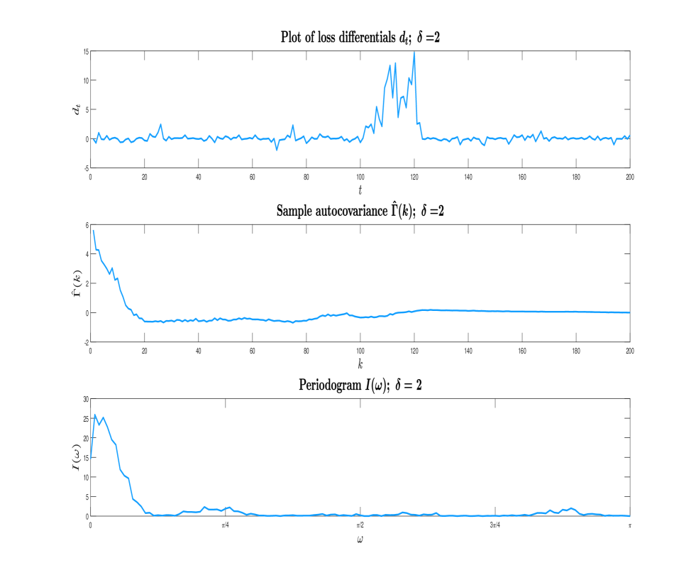
Figure S.1: a) top panel: plot of $\{d_{t}\};$ b) mid-panel: plot of the sample autocovariances $\widehat{\Gamma}\left(k\right)$ of $\{d_{t}\}$; c) bottom panel: plot the periodogram $I\left(\omega\right)$ of $\{d_{t}\}$. In all panels $\delta=2.$

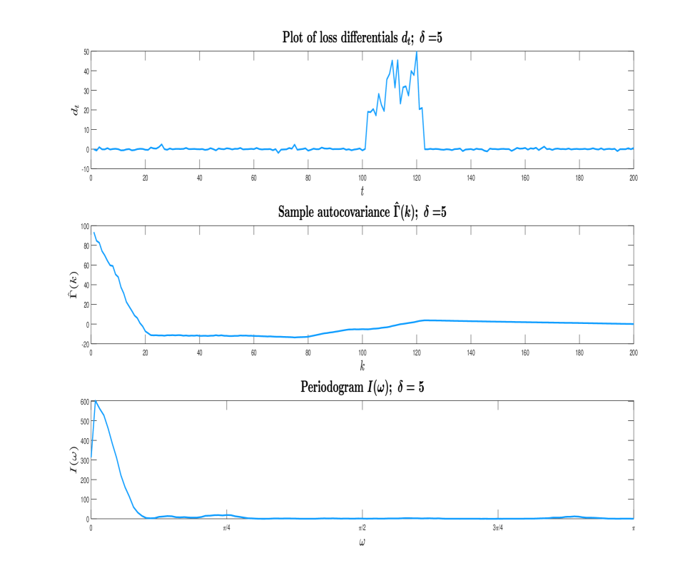
Figure S.2: a) top panel: plot of $\{d_{t}\};$ b) mid-panel: plot of the sample autocovariances $\widehat{\Gamma}\left(k\right)$ of $\{d_{t}\}$; c) bottom panel: plot the periodogram $I\left(\omega\right)$ of $\{d_{t}\}$. In all panels $\delta=5.$

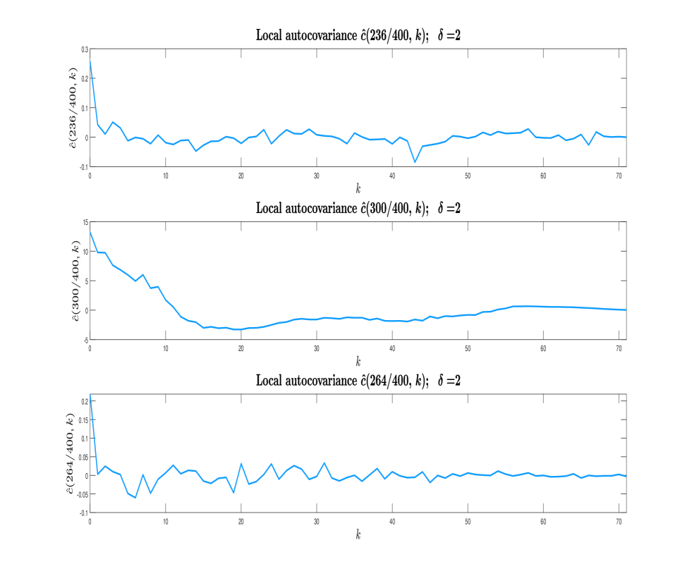
Figure S.3: The figure plots $\widehat{c}_{T}\left(u,\,k\right)$ for $u=236/400,\,\lambda_{1}^{0},\,264/400$ in the top, mid and bottom panel, respectively. In all panels $\delta=2.$

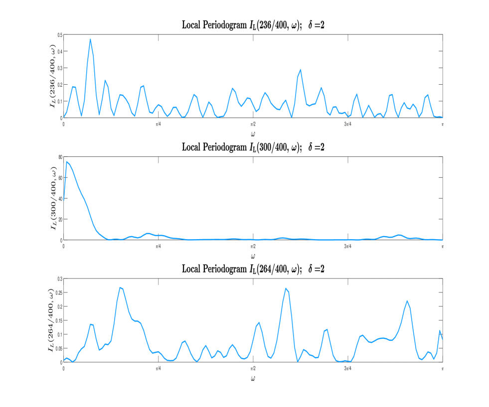
Figure S.4: The figure plots $I_{\mathrm{L}}\left(u,\,\omega\right)$ for $u=236/400,\,\lambda_{1}^{0},\,264/400$ in the top, mid and bottom panel, respectively. In all panels $\delta=2.$

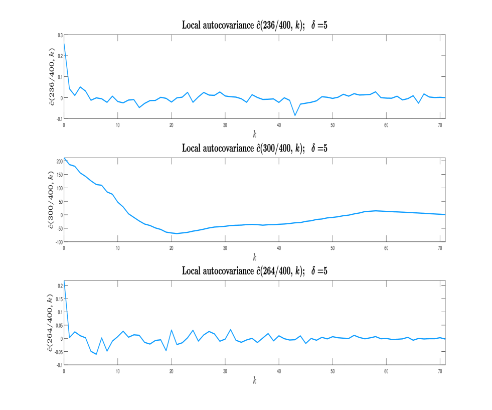
Figure S.5: The figure plots $\widehat{c}_{T}\left(u,\,k\right)$ for $u=236/400,\,\lambda_{1}^{0},\,264/400$ in the top, mid and bottom panel, respectively. In all panels $\delta=5.$

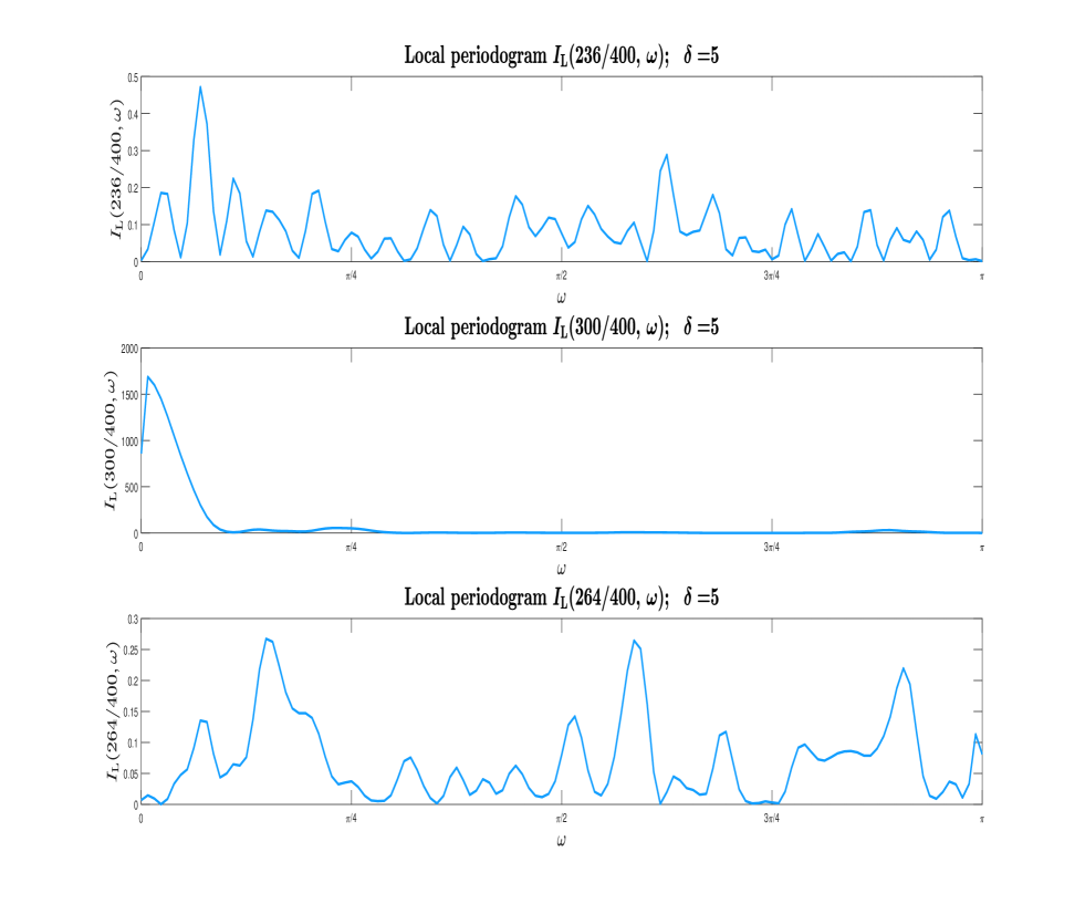
Figure S.6: The figure plots $I_{\mathrm{L}}\left(u,\,\omega\right)$ for $u=236/400,\,\lambda_{1}^{0},\,264/400$ in the top, mid and bottom panel, respectively. In all panels $\delta=5.$

elsarticle-harv References_Supp

References

- Altissimo and Corradi (2003) Altissimo, F., Corradi, V., 2003. Strong rules for detecting the number of breaks in a time series. Journal of Econometrics 117, 207–244.
- Andrews (1991) Andrews, D.W.K., 1991. Heteroskedasticity and autocorrelation consistent covariance matrix estimation. Econometrica 59, 817–858.
- Andrews (1993) Andrews, D.W.K., 1993. Tests for parameter instability and structural change with unknown change-point. Econometrica 61, 821–56.
- Andrews and Monahan (1992) Andrews, D.W.K., Monahan, J.C., 1992. An improved heteroskedasticity and autocorrelation consistent covariance matrix estimator. Econometrica 60, 953–966.
- Bai and Perron (1998) Bai, J., Perron, P., 1998. Estimating and testing linear models with multiple structural changes. Econometrica 66, 47–78.
- Belotti et al. (2021) Belotti, F., Casini, A., Catania, L., Grassi, S., Perron, P., 2021. Simultaneous bandwidths determination for double-kernel HAC estimators and long-run variance estimation in nonparametric settings. arXiv preprint arXiv:2103.00060.
- Bentkus and Rudzkis (1982) Bentkus, R.Y., Rudzkis, R.A., 1982. On the distribution of some statistical estimates of spectral density. Theory of Probability and Its Applications 27, 795–814.
- Bhattacharya et al. (1983) Bhattacharya, R., Gupta, V., Waymire, E., 1983. The Hurst effect under trends. Journal of Applied Probability 20, 649–662.
- Bhattacharya and Ghosh (1978) Bhattacharya, R.N., Ghosh, J.K., 1978. On the validity of the formal Edgeworth expansion. Annals of Statistics 6, 434–451.