Deep Learning strategies for ProtoDUNE raw data denoising

Abstract

In this work, we investigate different machine learning-based strategies for denoising raw simulation data from the ProtoDUNE experiment. The ProtoDUNE detector is hosted by CERN and it aims to test and calibrate the technologies for DUNE, a forthcoming experiment in neutrino physics. The reconstruction workchain consists of converting digital detector signals into physical high-level quantities. We address the first step in reconstruction, namely raw data denoising, leveraging deep learning algorithms. We design two architectures based on graph neural networks, aiming to enhance the receptive field of basic convolutional neural networks. We benchmark this approach against traditional algorithms implemented by the DUNE collaboration. We test the capabilities of graph neural network hardware accelerator setups to speed up training and inference processes.

1 Introduction

Deep learning algorithms achieved outstanding results in many research fields in the last few years. The neutrino high energy physics community domine2020 ; abi2020cnn ; aurisano2016 ; kronmueller2019 , and in general the particle physics one albertsson2019 ; bourilkov2019 , is making an effort to apply such technologies to create a new generation of automated tools. In general capable of processing efficiently huge amounts of information, these algorithms work with increased performance to mine deeper in collected data and discover hidden patterns responsible for potential new physics scenarios. Event reconstruction algorithms, i.e. reconstruction, the process of extraction of useful quantities from detector or simulated data, are especially suited to the application of this approach.

DUNE abi2020tdrI is a next-generation experiment in the neutrino oscillation research field. The DUNE Far Detector (FD) abi2020tdrII ; abi2020tdrIII ; abi2020tdrIV , based at the Sanford Underground Research Facility (SURF) in South Dakota, will be the largest monolithic Liquid Argon Time Projecting Chamber (LArTPC) detector ever built. In order to test and validate technologies for the construction of such detector, a prototype, ProtoDUNE Single Phase (SP) abi2017pdunetdr , has been built at the CERN Neutrino Platform.

Particle interactions with the liquid Argon produce ionization electrons that are drifted, thanks to an electric field, towards Anode Plane Assemblies (APAs) made of three readout planes that collect the deposited charge through time. Each readout plane is a bundle of wires, oriented in a specific direction and continuously monitored by the detector: two planes are called induction planes, while the last one is named the collection plane. In particular, the ProtoDUNE SP cage envelope is surrounded by 6 different APAs, each with two induction planes of 800 wires and a collection one, holding together 960 wires. Overall, a total of 15360 wires on the sides of the detector provide a comprehensive and detailed picture of events from different points of view.

ProtoDUNE SP measures a digitized value of the induced current on each wire (ADC value). Since the detector maximum sampling rate is $2\text{\,}\mathrm{MHz}$ and the common readout time windows at ProtoDUNE SP last $500\text{\,}\mathrm{ns}$, raw data (or raw digits) form a sequence of $6000$ current measurements per wire. In this paper we focus on event reconstruction of ProtoDUNE SP simulated data. We simulate interactions with the help of the LArSoft church2014larsoft framework and its dunetpc package. Figure 4, shows an example of the simulated data from a single collection plane: raw digits are cast into a $6000\times 960$ resolution image plotting the ADC values heat map over time versus wire number axes.

Raw digits recorded by detector electronics intrinsically contain noise that must be filtered out. The traditional approach abi2020tdrII , developed by the MicroBooNE experiment acciarri2017 ; adams2018 , is based on a 2-dimensional deconvolution and consists of two steps: first, a mask is produced to identify the Regions Of Interest (ROI) in the raw data containing signals; then, in those regions Gaussian shape peaks are fitted to match the inputs, filtering them in Fourier space and deconvolving back the results.

The goal of this work is to tackle the denoising problem, implementing automatic tools at the readout plane view level. The nature of the inputs, above all sparsity and size, represents a challenging benchmark for Deep Learning models. Images indeed contain signals, mainly organized in long monodimensional tracks and clusters, divided by almost empty extended regions. Then, trying to train classic deep feed-forward models on sparse inputs might lead to sub-optimal results, since gradients would receive a large contribution from pixels in those noise-dominated empty regions. Moreover, the high image resolution might result in a pixel receptive field limited to just local neighborhoods, which are small compared to the extension of the meaningful spatial features included in the plane views. Finally, handling the size of the inputs requires careful RAM and GPU memory management while dealing with complex model architectures.

The paper is organized as follows. First, in section 2 we describe the models and operations used to tackle the problem. Then, section 3 illustrates the dataset we generated and the methods employed to train the networks. Section 4 is devoted to the presentation of experimental results. Finally, in section 5 we present our conclusion and future development directions.

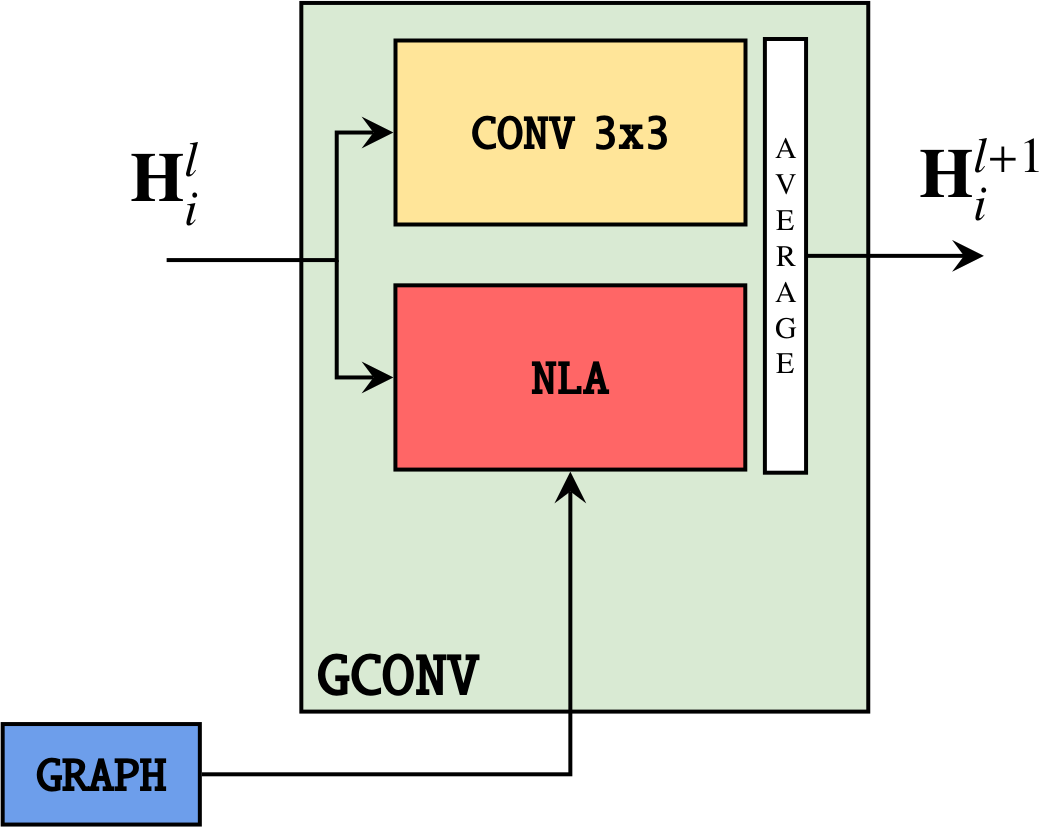
Figure 1: GCONV layer. The inner representation vector $\mathbf{H}^{l}_{i}$ is updated to $\mathbf{H}^{l+1}_{i}$ by means of NLA and 2D convolution operations. NLA relies on a previously computed KNN graph.

2 Proposed Models

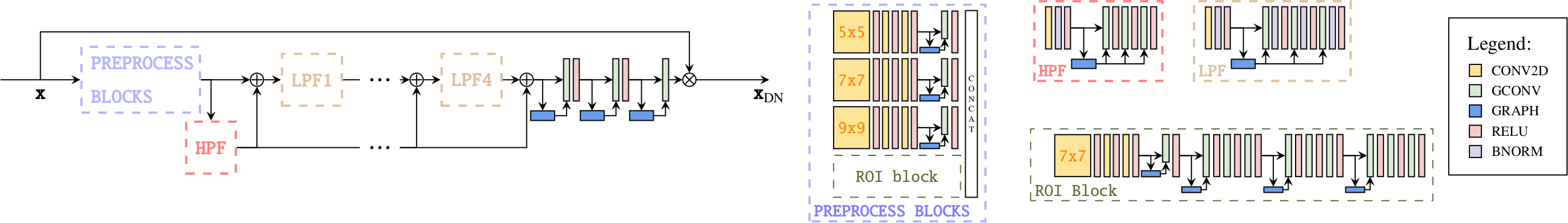
Figure 2: GCNN architecture. The model takes noisy input images x and outputs denoised ones x_DN. The design is organized with Low and High Pass Filters (LPF, HPF) as in valsesia2019deep . As explained in section 3.2, we concatenate a pretrained ROI block with preprocessing layers to make the network distinguish between signal and background. The ROI block, indeed, performs the binary segmentation.

Convolutional neural networks (CNN) are based on a stack of sliding kernels comprised of multiple filters, that are trained according to some optimization method to output a feature map. The convolutional kernel generates each feature map pixel as a function of a small neighboring portion of the input image. Hence, the receptive field of the pixels in each layer is constrained by the kernel size, which could be enlarged by increasing the depth of the network. The scope of the present section is to describe an alternative approach to the issue: by enriching the network with alternative operations we hope to increase the expressiveness of the internal representation by exploiting non-local correlations between pixel values, alongside the already discussed local neighborhood pixel intensities.

2.1 Graph Convolutional Neural Network

We implement a Graph Convolutional Neural Network (GraphCNN) inspired by valsesia2019image ; valsesia2019deep and based on the Edge Conditioned Convolution (ECC) operation, first presented in simonovsky2017dynamic . We employ a simplified version of the ECC layer: it builds the output representation as a pixel-wise average of a common convolution with a $3\times 3$ kernel and a Non-Local Aggregation (NLA) operation. We wrap such operations into a network layer called Graph Convolution (GCONV). Figure 1 sketches the GCONV layer mechanism.

The NLA connects each pixel to its $k$ closest ones in feature space, according to the Euclidean distance, and mixes the information through a feed-forward layer. If at layer $l$, the $i$-th of an $n$-pixel input image is described by the vector $\mathbf{H}^{l}_{i}\in\mathbb{R}^{d_{l}}$, then the NLA output $\mathbf{H}^{l+1}_{i}$ has the following form:

$$\scriptsize\mathbf{H}^{l+1}_{i}=\sigma\Biggl{(}\frac{1}{|\mathcal{N}_{i}^{l}|}\sum_{j\in\mathcal{N}_{i}^{l}}\mathrm{\Theta}^{l}\bigl{(}\mathbf{H}^{l}_{i}-\mathbf{H}^{l}_{j}\bigr{)}+\mathrm{W}^{l}\mathbf{H}^{l}_{i}+\mathbf{b}^{l}\Biggr{)}\hfill\in\mathbb{R}^{d_{l+1}}$$ (1)

With $\mathcal{N}_{i}^{l}$ being the neighborhood of pixel $i$ in the $H_{i}^{l}$ representation at layer $l$; $\{\mathrm{\Theta}^{l},W^{l}\}\in\mathbb{R}^{d_{l+1}\times d_{l}}$ and $\mathbf{b}^{l}\in\mathbb{R}^{d_{l}+1}$ are trainable weights and biases shared throughout pixels; $\sigma$ is the element-wise sigmoid function.

Note that the operation in equation 1 requires building a k-NN graph which requires an amount of memory proportional to the area of the input image times the number of neighbors per pixel $k$. Assuming we fix $k=8$, with an input image of $960\times 6000$ pixels and employing single precision floating point numbers, the graph construction operation burden is of order $\mathcal{O($200\text{\,}\mathrm{MB}$)}$. If the architecture involves multiple graph building operations, the GPU memory is easily saturated. Therefore, we have to limit the model inputs to just crops of the actual image as explained in section 3.2.

Figure 2 shows our GCNN network architecture. Note the final residual connection in the top branch: the usual sum has been replaced by a multiplication. This choice is tailor made on the input data themselves, which are mainly comprised of long tracks separated by empty space. In those regions it could be easier to learn how to remove the noise multiplicatively rather than additively. The network, in principle, doesn’t have to learn to perfectly profile the noise and then subtract it from the input itself, whereas it can employ a mask to cut down such uninteresting regions with multiplications by small numbers.

2.2 U-shaped Self Constructing Graph Network

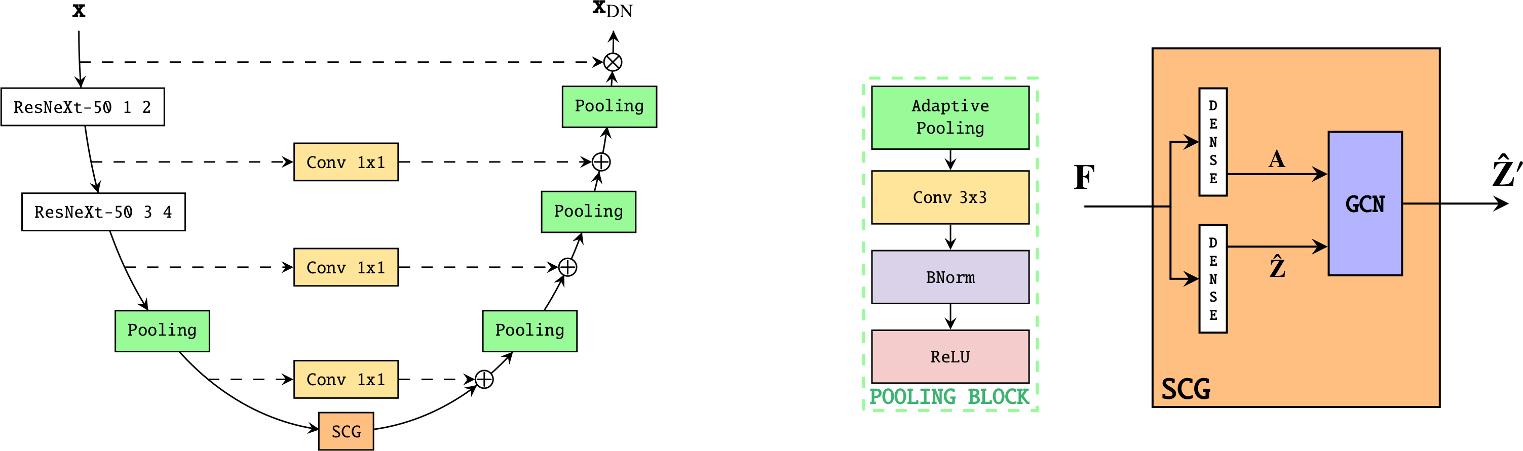
Figure 3: USCG-Net architecture. The Pooling block has a two folded aim thanks to its adaptive pooling layer: on the left branch it downscales the input, while on the right one it provides upsampling. According to xie2017aggregated , ResNeXt-50 with $32\times 4$ template is arranged in 4 main blocks, containing 9, 12, 18 and 9 convolutional layers respectively. In the chart we refer to such blocks as ResNeXt-50<block number> and we insert a residual connection between the second and the third block. The $1\times 1$ convolutions in the horizontal links are needed to adapt the number of filters in the image to perform the residual recombination operation.

As stated in the previous section, the main limitation of the GCNN model is the memory consuption burden due to the graph operation: graph building scales linearly with the size of the inputs, therefore, the model accepts crops rather than the full APA image. The cropping workaround prevents very long range correlations between pixels being taken into account and leads to inference time performance issues. If the user does not have access to a high GPU memory bandwidth, only batches of crops can be processed in parallel and processing big datasets is not time efficient.

As an alternative approach to the GCNN, we follow the idea introduced in liu2020scgnet with the Self Constructing Graph Network (SCG-Net): a graph neural network that outputs results from a low dimensional representation of the high resolution image created by a full CNN; the original shape of the image is then retrieved interpolating between pixels. In the original work, a bilinear interpolation is employed for the upsampling. In this way the authors were able to process big images containing up to $6000\times 6000$ pixels. This seems a more natural approach to the problem when the input images contain dense features, rather than sparse and localized ones as in our case. We believe that the entire pipeline potentially washes out the fine grained information contained in the input during downscaling, which cannot be recovered by means of a simple interpolation.

Therefore we introduce the U-shaped Self Constructing Graph Network (USCG-Net), where a U-Net ronneberger2015unet like network structure with residual connections carries the information from the input node all the way to the outputs. Figure 3 shows the USCG-Net architecture, with pooling blocks, comprised of convolutional and pooling layers, that take care of stepwise scaling the inputs. A pretrained ResNeXt-50 with a $32\times 4$ template xie2017aggregated is used to build an initial feature map to be fed into the SCG layer. The early-layer representation of the pretrained network should be generic enough to catch the spatial features of the inputs, driving the training process during the initial phases of the optimization. Note the residual recombination operations in the right branch: the sum in the residual connections has been replaced by a convolution with a $1\times 1$ kernel in order to increase the complexity of the network. Finally, for the final residual link, we employ again the multiplication trick, as explained in section 2.

The SGC layer is the core of the network: the input image is turned into a graph, allowing connections between distant pixels. The SCG layer liu2020scgnet takes in an image $\mathbf{F}\in\mathbb{R}^{h\times w\times d}$ and through an encoding functions, represented by dense layers, maps it into two outputs: an adjacency matrix $\mathbf{A}\in\mathbb{R}^{n\times n}$, describing the graph edges, and a node feature vector $\mathbf{\hat{Z}}\in\mathbb{R}^{n\times c}$. In the above formulas, $d$ and $c$ are the input and output channel dimensions respectively and $n$, which is equal to the input image resolution $h\times w$, is the number of extracted nodes. The predicted graph is then analyzed by a 1-layer graph neural network, such as GCN scarselli:2009 or GIN xu2019powerful , to further mix the node features, yielding a final node feature vector $\mathbf{\hat{Z}^{\prime}}\in\mathbb{R}^{n\times c^{\prime}}$. In our experiments we exploited the GCN layer as default; architecture variants with other kinds of graph layers can be addressed in a future work. $\mathbf{\hat{Z}^{\prime}}$ can be finally projected back into $\mathbb{R}^{h\times w\times c^{\prime}}$ and upsampled by pooling blocks in the right branch of the USCG-Net to the original image resolution.

3 Dataset and Training

3.1 Datsets

Table 1: Datasets for training and testing. The two differ in the producer package version, the size and the event beam energies. The second dataset contains $10$ events for each proton energy specified.

dunetpc	$n$ events	$p$ energy
v08_24_00	10	$2\text{\,}\mathrm{GeV}$
v09_10_00	70	$0.3\text{\,}\mathrm{GeV}$, $0.5\text{\,}\mathrm{GeV}$, $1\text{\,}\mathrm{GeV}$, $2\text{\,}\mathrm{GeV}$,
		$3\text{\,}\mathrm{GeV}$, $6\text{\,}\mathrm{GeV}$, $7\text{\,}\mathrm{GeV}$

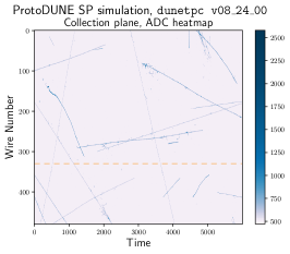
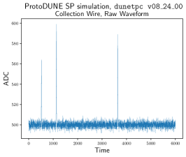
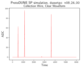
Figure 4: Example taken from dunetpc v08_24_00 dataset. Collection plane view with noisy and clear waveforms extracted from the channel marked by the horizontal orange dashed line.

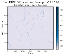
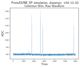
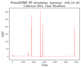
Figure 5: Example taken from dunetpc v09_10_00 dataset. Collection plane view with noisy and clear waveforms extracted from the channel marked by the horizontal orange dashed line.

In this section we present the datasets used to train and test our models. We underline that we present results for simulated data only, testing on detector data is out of the scope of the present work. We simulate interactions within the ProtoDUNE SP chamber through the LArSoft church2014larsoft framework and its dunetpc package. We consider events originating from a proton beam of various energies, plus cosmic rays, interacting with the Argon targets. Our supervised training approach is based on simulated raw digits. The simulation provides also the associated noise free charge depositions: we employ this information as target outputs for the denoising models.

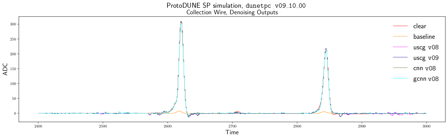
Figure 7: Detail of a raw waveform from dunetpc v09_10_00 dataset: label, traditional algorithm and neural networks outputs. The version, v08 or v09, next to the model name in the legend refers to which dataset the correspondent model was trained on.

Table 1 describes the considered datasets. In figures 4 and 5 we show visual examples from v08_24_00 and v09_10_00 datasets. We plot raw digit images and horizontal slices, namely single channel waveforms, either with (raw waveform) and without noise (clear waveform). Noise is mainly comprised of a pedestal value that changes across different datasets and a background noise that overwhelms small energy depositions and modifies spikes amplitudes. We consider the v08_24_00 dataset a simplified dataset since it is smaller and contains easier features to denoise and segment than the v09_10_00 one. v09_10_00 is more complex due to the detector data driven approach upon which the generator software is based. Clear waveforms are not simply zero in the empty regions, but rather contain small steps. Moreover, low frequency negative tails after big spikes in clear waveforms are clearly visible in figure 7.

We hold out from our datasets $10\%$ of images for validation and $10\%$ for testing. The validation set is used to choose the best model, while the test set is employed to present the final results given in section 4. The criterion chosen to present results is to aggregate each performance quantity, over the test or validation set, then report it as a symmetric interval with the central value and its uncertainty being the arithmetic mean and the standard deviation on the mean respectively. This choice also influences the best model selection during training, namely, the network checkpoint at epoch end that achieves the lowest upper bound of the loss function interval.

We remark that, as described in section 1, a single event at ProtoDUNE SP is recorded by 6 different APAs, that in turn provide 3 plane views. So one event does not count as one training point for our neural networks. In section 2, we anticipated that the GCNN network acts indipendently on small crops: if $32\times 32$ crops are employed, each event in the dataset becomes $9\times 10^{4}$ crops. The USCG-Net, instead, processes entire plane views. The two datasets provide $18$ and $126$ plane views to assess the model performance and its associated uncertainty. Note that the output image has a dimensionality of the order of millions of pixels and each pixel value provides a contribution in the computation of the final performance metric.

3.2 Network Training

All networks that we train share the same pre-processing procedure, where we take the plane views in a dataset and apply a median subtraction to each of them. This step is fundamental to estimate and subtract the pedestal value. We introduce this operation mimicking the traditional approach because it contributes to improve the final performance. Furthermore, for network training stability, the inputs are rescaled in the unit range according to the min-max normalization technique.

The GCNN network suffers from the memory issue discussed in section 2. To address this problem, we employ a data parallel approach, cropping the inputs into $32\times 32$ pixels images and processing every tile independently. However, this solution requires some subtleties in the training process due to the nature of the inputs.

Since the inputs contain sparse features, it is likely that the most of the crops contain little to no signal. It is meaningless to feed the the network with multiple empty crops. In order to speed up the training, we decide to train on just a subset of the available crops. This choice, in turn, triggers a second issue: sampling randomly the subset of crops provides an extremely unbalanced dataset, where we are very likely to miss crops containing interesting charge depositions. Hence, we fix the percentage of crops containing signal to balance the signal to background pixel ratio: in our experiments, we keep this quantity at $99\%$. The cropping procedure works as follows: we mark as signal all the pixels in clear waveforms that have non-zero ADC value count in a plane view; we sample randomly the desired number of crop centers, complying with the exact ratio of signal to background percentage; we finally crop the plane views around the drawn centers.

We train the GCNN network in figure 2 for both the image segmentation task and denoising, managed by the ROI Block and the network final outputs respectively. Image segmentation is a classification task at the pixel level, where the labels usually correspond to a finite set of exhaustive and mutually exclusive classes: the ROI block, indeed, is trained to distinguish between pixels that contain or not electron induced current signals. Image denoising, instead, aims at subtracting the noise contribution from each pixel intensity and is a regression task.

In order to optimize the two parts of the network, we design an ad-hoc training strategy as follows. First, we train the ROI Block alone on image segmentation for $100$ epochs and save the best configuration: in this step the network branch learns to distinguish between signal and background, i.e. empty pixels. We employ binary cross-entropy as the loss function, along with the AMSGrad variant j.2018on of the Adam algorithm kingma2017adam as the optimizer with a learning rate of $10^{-3}$. Second, we freeze and attach the trained ROI block weights to the remaining part of the network. Then, we train the GCNN on image denoising for a further $50$ epochs and save the network’s best configuration.

The GCNN denoising model is trained using the AMSGrad optimizer with a learning rate of $9\cdot 10^{-3}$, while optimizing a custom loss function made of two contributions: the mean squared error (MSE) $\mathcal{L}_{MSE}$ between labels and outputs and a loss function $\mathcal{L}_{ssim}$ derived from the statistical structural similarity index measure (stat-SSIM) chann:2008 . stat-SSIM for two images $\mathbf{x}$ and $\mathbf{y}$, is given by the following equation:

$$\mathrm{stat{\text{-}}SSIM}(\mathbf{x},\mathbf{y}) =\frac{1}{n_{p}n_{c}}\sum_{pc}\bigg{(}\frac{2\mu_{x}\mu_{y}+\epsilon_{\mu}}{\mu_{x}^{2}+\mu_{y}^{2}+\epsilon_{\mu}}\bigg{)}_{pc}$$ (2)

$$\times \bigg{(}\frac{2\mathrm{E}[(\mathbf{x}-\mu_{x})(\mathbf{y}-\mu_{y})]+\epsilon_{\sigma}}{\mathrm{E}[(\mathbf{x}-\mu_{x})^{2}]+\mathrm{E}[(\mathbf{y}-\mu_{y})^{2}]+\epsilon_{\sigma}}\bigg{)}_{pc}$$

where $\mu_{i}$ is a shorthand for the image $\mathbf{i}$ expected value $E[\mathbf{i}]$, which is computed through a convolution with a $11\times 11$ Gaussian kernel of standard deviation $3$. All the other expectation values in the equation are calculated convoluting the argument quantity with the same Gaussian filter. $\epsilon_{\mu}$ and $\epsilon_{\sigma}$ are two regulators that limit the maximum resolution at which the fractions in the equations are computed, respectively imposing a cut-off on the mean and variance expected values. In particular, when both the numerator and the denominator of a fraction reach much smaller values than the corresponding $\epsilon$, the output gets close to one. In the experiments, $\epsilon_{\mu}$ and $\epsilon_{\sigma}$ are fixed to the square of 0.5. This choice implies that for the stat-SSIM computation, we estimate the means and standard deviations of the distributions at scales larger than half of one ADC value, namely the granularity of the recorded detector hits. The result is finally averaged over the entire image containing $n_{p}$ pixels and $n_{c}$ channel dimensions. The quantity in equation 2 takes values in the range $[-1,1]$ and approaches $1$ only if $\mathbf{x}=\mathbf{y}$. The associated loss function is then given by $\mathcal{L}_{ssim}=1-\mathrm{stat{\text{-}}SSIM}$: it is a perceptual loss, in the sense that tries to assess the fidelity of the image focusing on structural information. It relies on the idea that pixels may have strong correlations, especially when they are spatially close. In contrast, MSE evaluates pixels’ absolute differences, without taking into account any dependence amongst them. More details on the interpretation of these quantities can be found in wang:2009mse . The two contributions in the loss function are weighted as follows: $\mathcal{L}=\alpha\cdot\mathcal{L}_{MSE}+(1-\alpha)\cdot w\cdot\mathcal{L}_{ssim}$. We fine tune the multiplicative parameter $w=10^{-3}$, to balance the gradients w.r.t. the model’s trainable parameters provided by the two terms in the sum. The parameter $\alpha$ is fixed to $0.84$ as in zhao2018loss .

In the following we will refer, with slight abuse of notation, to a CNN as a GCNN network with Graph Convolutional layers replaced by plain Convolutional ones.

The USCG-Net is relatively simple to train: since no crops are employed, no sampling method is required. Although no cropping is needed, since the model fits in a single $16\text{\,}\mathrm{GB}$ GPU even with an entire plane view as input, we prefer to employ a sliding window mechanism as in the original SCG-Net paper. We split the raw digits array along the time axis with a 2000 pixel wide window and 1000 pixel stride and feed each slice to the network. The results are then combined by averaging predictions on overlapping regions. The USCG-Net is trained minimizing the MSE function between model outputs and clear waveforms, with AMSGrad optimizer and learning rate of $10^{-3}$. In this case, we drop the stat-SSIM contribution from the loss function, since we experienced training convergence problems when including that term during our experiments.

4 Experiments results

We employ four different metrics to assess the goodness of our models and benchmark them against the state-of-the-art approach. Three of them are the stat-SSIM, peak signal to noise ratio (PSNR) and MSE on the two dimensional raw digits, while the last one is a custom metric called integrated mean absolute error (iMAE) and will be defined in the following.

PSNR between a noise-free image $\mathbf{x}$ and a denoised $\mathbf{y}$ one is given by the following equation:

$$\mathrm{PSNR}(\mathbf{x},\mathbf{y})=10\cdot\log_{10}\bigg{(}\frac{\max(\mathbf{x})^{2}}{\mathrm{MSE}(\mathbf{x},\mathbf{y})}\bigg{)}$$ (3)

Note that PSNR and stat-SSIM increase with the reconstruction quality, while MSE decreases. We observe that these three quantites are really suited to compare the deep learning models between themselves, however they are not really informative when the baseline approach is considered. Indeed, the baseline approach aims at fitting gaussian peaks in regions marked as interesting, rather than reconstructing the precise shape of the spike contained in the raw digits. Hence the baseline tool performs inevitably poorly on the considered metrics and up to our knowledge, there is no default metric to assess its performance. Nonetheless, we define a custom quantity that tries to compare the different approaches, observing that the deconvolution process does not preserve waveform amplitudes, but their integrals. For such reason we decide to evaluate the mean absolute error on wires integrated charge (iMAE):

$$\mathrm{iMAE}(\mathbf{x},\mathbf{y})=\frac{1}{n_{w}}\sum_{w=1}^{n_{w}}\Big{|}\sum_{t}(\mathbf{x}-\mathbf{y})_{wt}\Big{|}$$ (4)

where the sum inside the absolute values runs over time for the whole readout window, while the outer sum averages the result over the wire dimension. Note that the deconvolution approach does not preserve waveform amplitudes, because a filtering function is applied to the signal in Fourier space, then results are deconvolved back to the time domain. Furthermore, the deconvolution outputs are known up to an overall normalization constant, that we fit on the datasets in order to minimize the iMAE quantity. We show that, although we perform this operation on the state-of-the-art tool outputs for a fair comparison against our models, they nonetheless achieve a worse iMAE score. Table 2 collects the metrics values evaluated on v08_24_00 dataset. We gather v09_10_00 dataset results in table 3. Note that we present only evaluations for $2\text{\,}\mathrm{GeV}$ beam energy events, since we find metrics distributions to be flat in the energy parameter. Figures 6 and 7 show samples of labels and denoised waveforms.

USCG-Net like networks exceed GCNN-like ones in all the collected metrics. In order to have a first assessment of the quality of the neural network generalization power, we train two versions of the USCG-Net: one on the v08_24_00 dataset and the other on the v09_10_00 dataset. We decide not to train the GCNN-like networks on the v09_10_00 dataset after we observed difficulties in training convergence as well as long training times on such a big dataset. We evaluate these networks on both datasets.

Following expectations, the networks trained and applied on the same dataset lead to better performance. The only exceptions are given by the iMAE columns, where the USCG-Net trained on the dataset opposite to the testing one, achieve the best iMAE score. The stat-SSIM index score drops significantly for GCNN-like networks. All the networks, nonetheless, show hints of overall good generalization power when they are applied on datasets not used for training. This fact is well supported by the PSNR columns, which show that even the worst model achieves competitive results. We underline that the USCG-Net is not trained according to the stat-SSIM quantity: adding an extra term in the loss function containing such term could be considered a point of further development of the present research.

Table 2: Test metrics for denoising on v08_24_00 dataset. Results are shown for collection plane and $2\text{\,}\mathrm{GeV}$ beam energy only. The version, v08 or v09, next to the model name in the first column refers to which dataset the correspondent model was trained on.

Model	stat-SSIM	PSNR	MSE	iMAE
Baseline	-	-	-	$5391\pm 1622$
CNN v08	$0.471\pm 0.008$	$67.3\pm 1.2$	$0.57\pm 0.03$	$287\pm 12$
GCNN v08	$0.512\pm 0.011$	$70.12\pm 1.4$	$0.30\pm 0.01$	$191.4\pm 2.6$
USCG v08	$\bf 0.988\pm 0.005$	$\bf 72.66\pm 1.54$	$\bf 0.17\pm 0.02$	$95.5\pm 8.5$
USCG v09	$0.926\pm 0.007$	$72.3\pm 1.5$	$0.18\pm 0.02$	$\bf 76.3\pm 8.2$

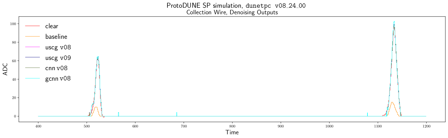
Figure 6: Detail of a raw waveform from dunetpc v08_24_00 dataset: label, traditional algorithm and neural networks outputs. The version, v08 or v09, next to the model name in the legend refers to which dataset the correspondent model was trained on.

Table 3: Test metrics for denoising on v09_10_00 dataset. Results are shown for collection plane and $2\text{\,}\mathrm{GeV}$ beam energy only. The version, v08 or v09, next to the model name in the first column refers to which dataset the correspondent model was trained on.

Model	stat-SSIM	PSNR	MSE	iMAE $[\times 10^{3}]$
Baseline	-	-	-	$5.86\pm 0.52$
CNN v08	$0.37\pm 0.02$	$57.3\pm 1.4$	$5.79\pm 0.88$	$4.16\pm 0.36$
GCNN v08	$0.40\pm 0.02$	$57.7\pm 1.5$	$5.27\pm 0.69$	$4.51\pm 0.39$
USCG v08	$0.65\pm 0.05$	$61.1\pm 1.6$	$2.3\pm 0.2$	$\bf 2.18\pm 0.29$
USCG v09	$\bf 0.81\pm 0.07$	$\bf 61.8\pm 1.7$	$\bf 1.99\pm 0.19$	$2.25\pm 0.23$

5 Conclusions

In this paper we presented Deep Learning strategies for denoising raw digits simulated data at ProtoDUNE SP. Our approach leads to an automated tool that cleans raw inputs and in the future could be adapted to work on real data. We investigated the capabilities of Graph Neural Networks, testing approaches alternative to classical Convolutional Neural Networks on a novel use case. Graph Neural Networks aimed to exploit long distance correlations between pixels, in particular the USCG-Net exemplified this approach, processing big sized inputs while still fitting GPU memory constraints. Our trained neural networks were able to outperform the state-of-the-art traditional reconstruction algorithm on the custom iMAE metric. All the networks gave hints of interesting generalization power, especially in the PSNR quality assessment, achieving high performances even on datasets different to the one they had been trained on. Further work directions will aim to fully assess the models on larger, more complete testing datasets.

Conflict of interest

The authors declare that they have no conflict of interest.

Data Availability Statement

This manuscript has associated data in a data repository. [Authors’ comment: No associated data except for code. The associated code to replicate the studies in this paper can be found at: this URL.

References

- (1) L. Dominé, K. Terao, Phys. Rev. D 102, 012005 (2020). DOI 10.1103/PhysRevD.102.012005. URL https://link.aps.org/doi/10.1103/PhysRevD.102.012005
- (2) B. Abi, R. Acciarri, et al., Phys. Rev. D 102, 092003 (2020). DOI 10.1103/PhysRevD.102.092003. URL https://link.aps.org/doi/10.1103/PhysRevD.102.092003
- (3) A. Aurisano, A. Radovic, et al., Journal of Instrumentation 11(09), P09001–P09001 (2016). DOI 10.1088/1748-0221/11/09/p09001. URL http://dx.doi.org/10.1088/1748-0221/11/09/P09001
- (4) M. Kronmueller, T. Glauch. Application of deep neural networks to event type classification in icecube. https://arxiv.org/abs/1908.08763 (2019)
- (5) K. Albertsson, P. Altoe, et al. Machine learning in high energy physics community white paper. https://arxiv.org/abs/1807.02876 (2019)
- (6) D. Bourilkov, International Journal of Modern Physics A 34(35), 1930019 (2019). DOI 10.1142/s0217751x19300199. URL http://dx.doi.org/10.1142/S0217751X19300199
- (7) B. Abi, R. Acciarri, et al., JINST 15(08), T08008 (2020). DOI 10.1088/1748-0221/15/08/T08008. URL https://doi.org/10.1088/1748-0221/15/08/T08008
- (8) B. Abi, R. Acciarri, et al. Deep underground neutrino experiment (dune), far detector technical design report, volume ii: Dune physics. https://arxiv.org/abs/2002.03005 (2020)
- (9) B. Abi, R. Acciarri, et al., JINST 15(08), T08009 (2020). DOI 10.1088/1748-0221/15/08/T08009. URL https://doi.org/10.1088/1748-0221/15/08/T08009
- (10) B. Abi, R. Acciarri, et al., JINST 15(08), T08010 (2020). DOI 10.1088/1748-0221/15/08/T08010. URL https://doi.org/10.1088/1748-0221/15/08/T08010
- (11) B. Abi, R. Acciarri, et al. The Single-Phase ProtoDUNE Technical Design Report. https://arxiv.org/abs/1706.07081 (2017)
- (12) E.D. Church. Larsoft: A software package for liquid argon time projection drift chambers. https://arxiv.org/abs/1311.6774 (2014)
- (13) R. Acciarri, C. Adams, et al., Journal of Instrumentation 12(08), P08003 (2017). DOI 10.1088/1748-0221/12/08/p08003. URL http://dx.doi.org/10.1088/1748-0221/12/08/P08003
- (14) C. Adams, R. An, et al., Journal of Instrumentation 13(07), P07006 (2018). DOI 10.1088/1748-0221/13/07/p07006. URL https://doi.org/10.1088/1748-0221/13/07/p07006
- (15) D. Valsesia, G. Fracastoro, et al. Deep graph-convolutional image denoising. https://arxiv.org/abs/1907.08448 (2019)
- (16) D. Valsesia, G. Fracastoro, et al. Image denoising with graph-convolutional neural networks. https://arxiv.org/abs/1905.12281 (2019)
- (17) M. Simonovsky, N. Komodakis. Dynamic edge-conditioned filters in convolutional neural networks on graphs. https://arxiv.org/abs/1704.02901 (2017)
- (18) S. Xie, R. Girshick, others, P. Dollár, Z. Tu, K. He. Aggregated residual transformations for deep neural networks. https://arxiv.org/abs/1611.05431 (2017)
- (19) Q. Liu, M. Kampffmeyer, et al. Scg-net: Self-constructing graph neural networks for semantic segmentation. https://arxiv.org/abs/2009.01599 (2020)
- (20) O. Ronneberger, P. Fischer, et al. U-net: Convolutional networks for biomedical image segmentation. https://arxiv.org/abs/1505.04597 (2015)
- (21) F. Scarselli, M. Gori, et al., IEEE Transactions on Neural Networks 20(1), 61 (2009). DOI 10.1109/TNN.2008.2005605. URL https://doi.org/10.1109/TNN.2008.2005605
- (22) K. Xu, W. Hu, et al. How powerful are graph neural networks? https://arxiv.org/abs/1810.00826 (2019)
- (23) S.J. Reddi, S. Kale, et al., in International Conference on Learning Representations (2018). URL https://openreview.net/forum?id=ryQu7f-RZ
- (24) D.P. Kingma, J. Ba. Adam: A method for stochastic optimization. https://arxiv.org/abs/1412.6980 (2017)
- (25) S.S. Channappayya, A.C. Bovik, et al., IEEE Transactions on Image Processing 17(6), 857 (2008). DOI 10.1109/TIP.2008.921328. URL https://doi.org/10.1109/TIP.2008.921328
- (26) Z. Wang, A.C. Bovik, IEEE Signal Processing Magazine 26(1), 98 (2009). DOI 10.1109/MSP.2008.930649. URL https://doi.org/10.1109/MSP.2008.930649
- (27) H. Zhao, O. Gallo, et al. Loss functions for neural networks for image processing. https://arxiv.org/abs/1511.08861 (2018)