Quantum entanglement in the anisotropic Heisenberg model with multicomponent DM and KSEA interactions

Abstract

Using group-theoretical approach we found a family of four nine-parameter quantum states for the two-spin-1/2 Heisenberg system in an external magnetic field and with multiple components of Dzyaloshinsky-Moriya (DM) and Kaplan-Shekhtman-Entin-Wohlman-Aharony (KSEA) interactions. Exact analytical formulas are derived for the entanglement of formation for the quantum states found. The influence of DM and KSEA interactions on the behavior of entanglement and on the shape of disentangled region is studied. A connection between the two-qubit quantum states and the reduced density matrices of many-particle systems is discussed.

1 Introduction

Quantum entanglement plays an important role in modern physics. It is not only used to test some fundamental questions of the quantum mechanics and quantum information processing but also widely employed in quantum computing NC00 ; VK02 ; V05 ; KM06 , communication E91 ; W98a ; GRTZ02 ; Pan20 , metrology PSOST18 , sensing DRC17 ; PBGWL18 , imaging LGB02 ; ZS20 , simulation of many-body systems F82 ; L96 ; JCJ14 ; ABC19 . All of these applications are largely dependent on how to produce entanglement.

Entanglement also affects the thermodynamic behavior of the system VA16 ; BCGAA18 ; DC19 ; OSMMN20 . According to classical thermodynamics, heat engines cyclically operating at a single temperature are not possible, the maximum efficiency of any heat engine is limited by the Carnot bound, etc. In contrast, in quantum thermodynamics, engines that operate at a single temperature are proposed SZAW03 ; G07 ; YTK17 , entangled thermal systems that can be more efficient in extracting work than the systems without quantum correlations are considered BACRR17 ; AMVSSOA19 ; CCA20 , emergence of the second law of thermodynamics is discussed LY99 ; CSHO15 ; KLSVBL18 ; BLB19 .

Quantitative measures for the quantum entanglement of bipartite systems were introduced by Bennett et al. in 1996, first for pure states BBPS96 and then for mixed ones BDSW96 . These measures are based on entropy and, for mixed states, involve the extremization procedure to find the optimal ensemble. Unfortunately, the problems of extemization are known to be very difficult to handle analytically, and apparently therefore the authors BDSW96 were able to obtain an exact expression for the entanglement of formation only in the case of Bell-diagonal states. The next important step was taken by Wootters who proved a conjecture of Hill and Wootters HW97 , which gives an explicit prescription for evaluating the entanglement of any two-qubit system. However, the Wootters formula (see Sect. 2) requires a solution of fourth degree algebraic equation, that is, the use of extremely cumbersome Ferrari’s formulas. Therefore, for practical purposes, it is important to derive compact expressions for different particular types of quantum states. For instance, in Ref. CW01 , a formula for the two-qubit block-diagonal (XXZ) state was presented and used. Then this formula was generalized to the arbitrary X quantum state YE07 . In Ref. FKY12 , an explicit expression was also obtained for the entanglement of a centrosymmetric (CS) quantum state.

Recently, a family of fifteen quantum states was found, for which the problem of calculating quantum correlations is reduced to solving quadratic equations Y20 . This family contains three different types of anisotropic Heisenberg spin systems with one-component Dzyaloshinsky-Moriya (DM) and Kaplan-Shekhtman-Entin-Wohlman-Aharony (KSEA) interactions. In the present paper we give a collection of four two-qubit XYZ models that extend the DM-KSEA interactions to several components. A classification was performed by using group-theoretical methods. The solutions in these cases are reduced to solving cubic algebraic equations. Using the well-known trigonometric form for the real roots of such equations, we get closed analytical formulas for the quantum entanglement.

The following should be noted. A distinctive feature of entanglement in comparison with other quantum correlations, such as discord, is that in the process of evolution in some parameter (time, temperature, etc.) it can suddenly disappear N98 ; ABV01 ; YE04 . This phenomenon is called the entanglement sudden death (ESD) YE06 ; YE09 . Moreover, entanglement can not only suddenly disappear, but also suddenly appear again YE09 ; FT10 ; WHH18 ; SG20 . Below we will present the behavior of quantum entanglement and the shape of the separability region in the presence of DM and KSEA interactions.

The remainder of the paper is organized as follows. In the next section (Sect. 2), we recall the notions and some facts necessary for further consideration. Symmetries and corresponding family of quantum states are given in Sect. 3. Next, in Sect. 4, the analytical formulas for the quantum entanglement of the states found are derived. The results are discussed in Sect 5. Finally, concluding remarks are provided in Sect. 6.

2 Preliminaries

The entanglement of formation of a two-qubit quantum state $\rho$ ($\rho^{\dagger}=\rho,\ \rho\geq 0,\ {\rm tr}\rho=1$) is given as

$${\rm EoF}(\rho)=-\frac{1+\sqrt{1-C^{2}}}{2}\log_{2}\frac{1+\sqrt{1-C^{2}}}{2}-\frac{1-\sqrt{1-C^{2}}}{2}\log_{2}\frac{1-\sqrt{1-C^{2}}}{2},$$ (1)

where $C$ is the concurrence. It is important that the concurrence can also serve as a measure of quantum correlation. Wootters W98 strongly proved that the concurrence of an arbitrary state of two qubits equals

$$C(\rho)=\max\{0,\sqrt{\lambda_{1}}-\sqrt{\lambda_{2}}-\sqrt{\lambda_{3}}-\sqrt{\lambda_{4}}\},$$ (2)

where $\lambda_{i}$ are the eigenvalues (ordered as $\lambda_{i}\geq\lambda_{i+1}$) of the $4\times 4$-matrix

$$R=\rho\tilde{\rho},$$ (3)

in which

$$\tilde{\rho}=(\sigma_{y}\otimes\sigma_{y})\rho^{*}(\sigma_{y}\otimes\sigma_{y})$$ (4)

is the spin-flipped state. Here, $\sigma_{y}$ is the Pauli spin $y$-matrix in standard basis and the asterisk denotes complex conjugation.

The matrix $\sigma_{y}\otimes\sigma_{y}=V$ ($V^{-1}=V$) in Eq. (4) acts as a similarity transformation. Since $\rho$ is positive operator, the matrix $\tilde{\rho}$ is also positive and their product $R$, generally non-Hermitian, will have only real and non-negative eigenvalues. Notice in passing the equality $\det R=\det(\rho\tilde{\rho})=(\det\rho)^{2}$.

Further, we will keep in mind that the density matrices come from the equilibrium statistical mechanics of a system with Hamiltonian $\cal H$, i.e., it is the Gibbs density matrix

$$\rho=\frac{1}{Z}e^{-\beta{\cal H}}$$ (5)

($Z$ is the partition function and $\beta$ the inverse temperature) or, say, equals the time-dependent density matrix

$$\rho(t)=e^{-i{\cal H}t}\rho(0)e^{i{\cal H}t},$$ (6)

which follows from the quantum Liouville-von Neumann equation, provided that the initial state $\rho(0)$ belongs to the same symmetry class as the Hamiltonian. In these cases, the Hamiltonian and corresponding density matrix commute: $[\rho,{\cal H}]=0$. As a result, they can be expanded in terms of the same set of spin operators.

The most general Hamiltonian of two-qubit system can be written as

$${\cal H}={\cal H}_{\rm Z}+{\cal H}_{\rm H}+{\cal H}_{\rm DM}+{\cal H}_{\rm KSEA}.$$ (7)

Here ${\cal H}_{\rm Z}$ is the Zeeman energy, ${\cal H}_{\rm H}$ denotes the Heisenberg exchange couplings, the third term

$${\cal H}_{\rm DM}={\bf D}\!\cdot\!({\vec{\sigma}}_{1}\times{\vec{\sigma}}_{2})$$

$$=D_{x}(\sigma_{1}^{y}\sigma_{2}^{z}-\sigma_{1}^{z}\sigma_{2}^{y})+D_{y}(\sigma_{1}^{z}\sigma_{2}^{x}-\sigma_{1}^{x}\sigma_{2}^{z})+D_{z}(\sigma_{1}^{x}\sigma_{2}^{y}-\sigma_{1}^{y}\sigma_{2}^{x})$$ (8)

is the DM interaction, in which ${\bf D}=(D_{x},D_{y},D_{z})$ is the Dzyaloshinsky vector and $\vec{\sigma}_{i}=(\sigma_{i}^{x},\sigma_{i}^{y},\sigma_{i}^{z})$ the vector of Pauli spin matrices at site $i$ ($=1,2$), and the last term

$${\cal H}_{\rm KSEA}={\vec{\sigma}}_{1}\!\cdot\!\hat{\rm\Gamma}\!\cdot\!{\vec{\sigma}}_{2}\equiv(\sigma_{1}^{x},\sigma_{1}^{y},\sigma_{1}^{z})\left(\begin{array}[]{ccc}.&{\rm\Gamma}_{z}&{\rm\Gamma}_{y}\\ {\rm\Gamma}_{z}&.&{\rm\Gamma}_{x}\\ {\rm\Gamma}_{y}&{\rm\Gamma}_{x}&.\end{array}\right)\!\left(\begin{array}[]{c}\sigma_{2}^{x}\\ \sigma_{2}^{y}\\ \sigma_{2}^{z}\end{array}\right)$$ (15)

$$={\rm\Gamma}_{x}(\sigma_{1}^{y}\sigma_{2}^{z}+\sigma_{1}^{z}\sigma_{2}^{y})+{\rm\Gamma}_{y}(\sigma_{1}^{z}\sigma_{2}^{x}+\sigma_{1}^{x}\sigma_{2}^{z})+{\rm\Gamma}_{z}(\sigma_{1}^{x}\sigma_{2}^{y}+\sigma_{1}^{y}\sigma_{2}^{x})$$ (16)

represents the KSEA interaction, where ${\hat{\rm\Gamma}}$ is a symmetric traceless tensor; the points are put instead of zero entries. So, in the general case, both the DM and KSEA interactions have three components each.

3 Symmetries and a family of quantum states

In open form,

$$V\equiv\sigma_{y}\otimes\sigma_{y}=\left(\begin{array}[]{rrrr}.&.&.&-1\\ .&.&1&.\\ .&1&.&.\\ -1&.&.&.\end{array}\right)=V^{T},$$ (17)

where the subscript $T$ stands for matrix transpose.

The starting point of our approach is as follows. We will find the symmetries of matrix (17) and then impose the same symmetry on the state $\rho$. In this case, the matrix

$$R=\rho\cdot V^{T}\rho^{*}V$$ (18)

is invariant under the taken symmetry. Further we will use the apparatus of group theory to reduce the matrix $R$ to block-diagonal form and thereby simplify the problem of extracting its eigenvalues. Of course, we need to dwell on such symmetries that lead to new results. For example, matrix (17) is invariant under transformations $\sigma_{x}\otimes\sigma_{x}$, $\sigma_{y}\otimes\sigma_{y}$, and $\sigma_{z}\otimes\sigma_{z}$, but we exclude these symmetries, because they have already been described in Ref. Y20 .

3.1 Symmetry groups

It is clear that the matrix (17) is invariant under simultaneous permutations of the second and third rows and columns (transformation $P_{23}$) or, conversely, under permutations of the first and fourth rows and columns (transformation $P_{14}$). In an explicit form

$$P_{23}=\left(\begin{array}[]{rrrr}1&.&.&.\\ .&.&1&.\\ .&1&.&.\\ .&.&.&1\end{array}\right)=P_{23}^{T}$$ (19)

and

$$P_{14}=\left(\begin{array}[]{rrrr}.&.&.&1\\ .&1&.&.\\ .&.&1&.\\ 1&.&.&.\end{array}\right)=P_{14}^{T}.$$ (20)

Moreover, we also observed that the matrix (17) remains unchanged under two other orthogonal transformations

$$P_{\bar{2}\bar{3}}=\left(\begin{array}[]{rrrr}1&.&.&.\\ .&.&-1&.\\ .&-1&.&.\\ .&.&.&1\end{array}\right)=P_{\bar{2}\bar{3}}^{T}$$ (21)

and

$$P_{\bar{1}\bar{4}}=\left(\begin{array}[]{rrrr}.&.&.&-1\\ .&1&.&.\\ .&.&1&.\\ -1&.&.&.\end{array}\right)=P_{\bar{1}\bar{4}}^{T}$$ (22)

Obviously that the squares of matrices (19)-(22) equal unity. Each of these four transformations together with the unit element $E$ compose the groups $\{E,P_{23}\}$, $\{E,P_{14}\}$, $\{E,P_{\bar{2}\bar{3}}\}$, and $\{E,P_{\bar{1}\bar{4}}\}$. Below we sometimes use the collective notation $P=\{P_{23},P_{14},P_{\bar{2}\bar{3}},P_{\bar{1}\bar{4}}\}$ for the permutation transformations.

3.2 Group-theoretical analysis

To know simplifications for the initial task due to symmetries, we perform a group-theoretical analysis. Each of groups $\{E,P\}$ has the second order and has two irreducible representations ${\rm\Gamma}^{(1)}$ and ${\rm\Gamma}^{(2)}$. The $4\times 4$ unit matrix and any matrix $P$ together give the original representation $\rm\Gamma$ of the taken group in the space of density matrix. The characters of $\rm\Gamma$ (traces of representation matrices) equal $\chi(E)=4$ and $\chi(P_{23})=\chi(P_{14})=\chi(P_{\bar{2}\bar{3}})=\chi(P_{\bar{1}\bar{4}})=2$. Knowing them we can find the multiplicities $a_{1}$ and $a_{2}$ with which the irreducible representations ${\rm\Gamma}^{(1)}$ and ${\rm\Gamma}^{(2)}$, respectively, are contained in $\rm\Gamma$.

Table 1: Character table of the group $\{E,P\}$

$\{E,P\}$	$E$	$P$
${\rm\Gamma}^{(1)}$	$1$	$1$
${\rm\Gamma}^{(2)}$	$1$	$-1\ \$
$\rm\Gamma$	$4$	$2$

For this purpose it is sufficient to use of the character table for the group (Table 1) and the formula LL_QM65 ; H62

$$a_{\mu}=\frac{1}{g}\sum_{G}\chi(G)\chi^{(\mu)^{*}}(G),$$ (23)

where $g$ is the order of the group, $\chi^{(\mu)}(G)$ the character of the element $G$ in the $\mu$-th irreducible representation, and $\chi(G)$ the character of the same element in the representation under question. Simple calculations yield

$$a_{1}=3,\qquad a_{2}=1.$$ (24)

This means that in the basis where the representation $\rm\Gamma$ of the Abelian group $\{E,P\}$ is completely reduced, the density matrices will take a block-diagonal form with one subblock $3\times 3$ and one “subblock” $1\times 1$.

The eigenvalues of the matrices $P$ are equal to $+1$ which is threefold degenerate and to $-1$. The eigenvectors are

$$|\Phi^{+}\rangle=\frac{1}{\sqrt{2}}\left(\begin{array}[]{c}1\\ .\\ .\\ 1\end{array}\right),|\Phi^{-}\rangle=\frac{1}{\sqrt{2}}\left(\begin{array}[]{c}1\\ .\\ .\\ -1\end{array}\right),|\Psi^{+}\rangle=\frac{1}{\sqrt{2}}\left(\begin{array}[]{c}.\\ 1\\ 1\\ .\end{array}\right),|\Psi^{-}\rangle=\frac{1}{\sqrt{2}}\left(\begin{array}[]{c}.\\ 1\\ -1\\ .\end{array}\right)$$ (25)

(these are the Bell states). The given eigenvectors are the same for all $P$-operators (and also for $V$), but the eigenvectors which corresponds to the non-degenerate eigenvalue $-1$ are different for each $P$-matrix. Vector $|\Psi^{-}\rangle$ in set (25) corresponds to the operator $P_{23}$, $|\Phi^{-}\rangle$ to $P_{14}$, $|\Psi^{+}\rangle$ to $P_{\bar{2}\bar{3}}$, and $|\Phi^{+}\rangle$ to $P_{\bar{1}\bar{4}}$.

Quasi-diagonalizing transformations are constructed from the eigenvectors of the operators $P$. Such a transformation for the operator $P_{23}$ can be written as

$$O_{23}=\frac{1}{\sqrt{2}}\left(\begin{array}[]{ccrr}.&1&1&.\\ 1&.&.&1\\ 1&.&.&-1\\ .&1&-1&.\end{array}\right)=O_{23}^{T}.$$ (26)

This transformation is orthogonal and symmetric. Likewise for other operators $P$:

$$O_{14}=\frac{1}{\sqrt{2}}\left(\begin{array}[]{ccrr}1&.&.&1\\ .&1&1&.\\ .&1&-1&.\\ 1&.&.&-1\end{array}\right)=O_{14}^{T},$$ (27)

$$O_{\bar{2}\bar{3}}=\frac{1}{\sqrt{2}}\left(\begin{array}[]{ccrr}.&1&1&.\\ 1&.&.&1\\ -1&.&.&1\\ .&1&-1&.\end{array}\right),$$ (28)

and

$$O_{\bar{1}\bar{4}}=\frac{1}{\sqrt{2}}\left(\begin{array}[]{ccrr}1&.&.&1\\ .&1&1&.\\ .&1&-1&.\\ -1&.&.&1\end{array}\right).$$ (29)

The last columns in the matrices (26)–(29) equal the eigenvectors corresponding the eigenvalue $-1$. Such an arrangement of columns provides a direct sum structure $3\oplus 1$ for the density matrices after their quasi-diagonalizations.

Let us now turn to the consideration of models with four symmetries separately.

3.3 Construction of quantum states

The most general matrix which commutes with the operator (19) has the following form

$$A=\left(\begin{array}[]{cccc}A_{1}&A_{2}&A_{2}&A_{3}\\ A_{4}&A_{5}&A_{6}&A_{7}\\ A_{4}&A_{6}&A_{5}&A_{7}\\ A_{8}&A_{9}&A_{9}&A_{10}\end{array}\right),$$ (30)

where $A_{1},\ldots,A_{10}$ are arbitrary real or complex numbers. This matrix remains unchanged while permuting the second and third rows and columns (for brevity, it can be called a $\pi_{23}$-matrix).

Since the density matrix must be Hermitian, the most general form of density matrix that commutes with $P_{23}$ is written as

$$\rho_{23}=\left(\begin{array}[]{cccc}a&\mu&\mu&\nu\\ \mu^{*}&b&c&\gamma\\ \mu^{*}&c&b&\gamma\\ \nu^{*}&\gamma^{*}&\gamma^{*}&d\end{array}\right).$$ (31)

Here and below, the Latin letters $a$, $b$, $c$, and $d$ for the entries in density matrices are real, whereas the Greek letters $\mu$, $\nu$, and $\gamma$ can be complex. Since for any density matrix ${\rm tr}\rho=1$, the matrix (31) contains nine real parameters.

Bloch decomposition of the density matrix (31) is written as

$$\rho_{23}=\frac{1}{4}[1+s_{x}(\sigma_{1}^{x}+\sigma_{2}^{x})+s_{y}(\sigma_{1}^{y}+\sigma_{2}^{y})+s_{z}(\sigma_{1}^{z}+\sigma_{2}^{z})+c_{1}\sigma_{1}^{x}\sigma_{2}^{x}+c_{2}\sigma_{1}^{y}\sigma_{2}^{y}$$

$$+c_{3}\sigma_{1}^{z}\sigma_{2}^{z}+g_{x}(\sigma_{1}^{y}\sigma_{2}^{z}+\sigma_{1}^{z}\sigma_{2}^{y})+g_{y}(\sigma_{1}^{x}\sigma_{2}^{z}+\sigma_{1}^{z}\sigma_{2}^{x})+g_{z}(\sigma_{1}^{x}\sigma_{2}^{y}+\sigma_{1}^{y}\sigma_{2}^{x})].$$ (32)

This matrix in open form looks as

$$\rho_{23}=\frac{1}{4}\left(\begin{array}[]{cccc}1+2s_{z}+c_{3}&s_{x}+g_{y}&s_{x}+g_{y}&c_{1}-c_{2}-2ig_{z}\\ &-i(s_{y}+g_{x})&\ -i(s_{y}+g_{x})&\\ \\ s_{x}+g_{y}&1-c_{3}&c_{1}+c_{2}&s_{x}-g_{y}\\ +i(s_{y}+g_{x})&&&-i(s_{y}-g_{x})\\ \\ s_{x}+g_{y}&c_{1}+c_{2}&1-c_{3}&s_{x}-g_{y}\\ +i(s_{y}+g_{x})&&&-i(s_{y}-g_{x})\\ \\ c_{1}-c_{2}+2ig_{z}&s_{x}-g_{y}&s_{x}-g_{y}&1-2s_{z}+c_{3}\\ &+i(s_{y}-g_{x})&\ +i(s_{y}-g_{x})&\end{array}\right).$$ (33)

Comparing Eqs. (31) and (33) one find relation between parameters of the quantum state $\rho_{23}$ in different forms,

$$a=(1+2s_{z}+c_{3})/4,\quad b=(1-c_{3})/4,\quad c=(c_{1}+c_{2})/4,$$

$$d=(1-2s_{z}+c_{3})/4,\quad\mu=(s_{x}+g_{y})/4-i(s_{y}+g_{x})/4,$$ (34)

$$\nu=(c_{1}-c_{2})/4-ig_{z}/2,\quad\gamma=(s_{x}-g_{y})/4-i(s_{y}-g_{x})/4.$$

Here, nine real parameters $s_{x}$, $s_{y}$, $s_{z}$, $c_{1}$, $c_{2}$, $c_{3}$, $g_{x}$, $g_{y}$, and $g_{z}$ equal unary and binary correlation functions and can vary from $-1$ to $+1$. The Hamiltonian with the same algebraic structure reads

$${\cal H}_{23}={\bf B}\!\cdot\!(\vec{\sigma}_{1}+\vec{\sigma}_{2})+J_{x}\sigma_{1}^{x}\sigma_{2}^{x}+J_{y}\sigma_{1}^{y}\sigma_{2}^{y}+J_{z}\sigma_{1}^{z}\sigma_{2}^{z}+{\vec{\sigma}}_{1}\!\cdot\!\hat{\rm\Gamma}\!\cdot\!{\vec{\sigma}}_{2},$$ (35)

where ${\bf B}=(B_{x},B_{y},B_{z})$ is an external magnetic field with arbitrary orientation, $J_{\alpha}$ ($\alpha=x,y,z$) are the Heisenberg coupling constants, and the last term represents the complete KSEA interactions.

Acting in a similar manner, we obtain density matrices and corresponding Hamiltonians for the systems with other three symmetries. Commutativity condition of Hermitian matrix with the $P_{14}$ leads to the $\pi_{14}$ quantum state:

$$\rho_{14}=\left(\begin{array}[]{cccc}a&\mu&\nu&d\\ \mu^{*}&b&\gamma&\mu^{*}\\ \nu^{*}&\gamma^{*}&c&\nu^{*}\\ d&\mu&\nu&a\end{array}\right)= \frac{1}{4}[1+s_{x}(\sigma_{1}^{x}+\sigma_{2}^{x})+s_{y}(\sigma_{1}^{y}-\sigma_{2}^{y})+s_{z}(\sigma_{1}^{z}-\sigma_{2}^{z})$$ (41)

$$+c_{1}\sigma_{1}^{x}\sigma_{2}^{x}+c_{2}\sigma_{1}^{y}\sigma_{2}^{y}+c_{3}\sigma_{1}^{z}\sigma_{2}^{z}+g_{x}(\sigma_{1}^{y}\sigma_{2}^{z}+\sigma_{1}^{z}\sigma_{2}^{y})$$

$$+\delta_{y}(\sigma_{1}^{z}\sigma_{2}^{x}-\sigma_{1}^{x}\sigma_{2}^{z})+\delta_{z}(\sigma_{1}^{x}\sigma_{2}^{y}-\sigma_{1}^{y}\sigma_{2}^{x})],$$

where $s_{x}$, $s_{y}$, $s_{z}$, $c_{1}$, $c_{2}$, $c_{3}$, $g_{x}$, $\delta_{y}$, and $\delta_{z}$ are nine real parameters; they also have the physical meaning of correlation functions. The Hamiltonian of the system is written as

$${\cal H}_{14}=B_{x}(\sigma_{1}^{x}+\sigma_{2}^{x})+B_{y}(\sigma_{1}^{y}-\sigma_{2}^{y})+B_{z}(\sigma_{1}^{z}-\sigma_{2}^{z})+J_{x}\sigma_{1}^{x}\sigma_{2}^{x}+J_{y}\sigma_{1}^{y}\sigma_{2}^{y}$$

$$+J_{z}\sigma_{1}^{z}\sigma_{2}^{z}+{\rm\Gamma}_{x}(\sigma_{1}^{y}\sigma_{2}^{z}+\sigma_{1}^{z}\sigma_{2}^{y})+D_{y}(\sigma_{1}^{x}\sigma_{2}^{z}-\sigma_{1}^{z}\sigma_{2}^{x})+D_{z}(\sigma_{1}^{x}\sigma_{2}^{y}-\sigma_{1}^{y}\sigma_{2}^{x})].\quad\$$ (42)

For the system with $P_{\bar{2}\bar{3}}$-symmetry the density matrix is given by

$$\rho_{\bar{2}\bar{3}}=\frac{1}{4}[1+s_{x}(\sigma_{1}^{x}-\sigma_{2}^{x})+s_{y}(\sigma_{1}^{y}-\sigma_{2}^{y})+s_{z}(\sigma_{1}^{z}+\sigma_{2}^{z})+c_{1}\sigma_{1}^{x}\sigma_{2}^{x}+c_{2}\sigma_{1}^{y}\sigma_{2}^{y}$$

$$+c_{3}\sigma_{1}^{z}\sigma_{2}^{z}+\delta_{x}(\sigma_{1}^{y}\sigma_{2}^{z}-\sigma_{1}^{z}\sigma_{2}^{y})+\delta_{y}(\sigma_{1}^{z}\sigma_{2}^{x}-\sigma_{1}^{x}\sigma_{2}^{z})+g_{z}(\sigma_{1}^{x}\sigma_{2}^{y}+\sigma_{1}^{y}\sigma_{2}^{x})]$$ (43)

and corresponding Hamiltonian is

$${\cal H}_{\bar{2}\bar{3}}=B_{x}(\sigma_{1}^{x}-\sigma_{2}^{x})+B_{y}(\sigma_{1}^{y}-\sigma_{2}^{y})+B_{z}(\sigma_{1}^{z}+\sigma_{2}^{z})+J_{x}\sigma_{1}^{x}\sigma_{2}^{x}+J_{y}\sigma_{1}^{y}\sigma_{2}^{y}$$

$$+J_{z}\sigma_{1}^{z}\sigma_{2}^{z}+D_{x}(\sigma_{1}^{y}\sigma_{2}^{z}-\sigma_{1}^{z}\sigma_{2}^{y})+D_{y}(\sigma_{1}^{x}\sigma_{2}^{z}-\sigma_{1}^{z}\sigma_{2}^{x})+{\rm\Gamma}_{z}(\sigma_{1}^{x}\sigma_{2}^{y}-\sigma_{1}^{y}\sigma_{2}^{x})].\quad\$$ (44)

Finally, for the system with $P_{\bar{1}\bar{4}}$-symmetry quantum state is written as

$$\rho_{\bar{1}\bar{4}}=\frac{1}{4}[1+s_{x}(\sigma_{1}^{x}-\sigma_{2}^{x})+s_{y}(\sigma_{1}^{y}+\sigma_{2}^{y})+s_{z}(\sigma_{1}^{z}-\sigma_{2}^{z})+c_{1}\sigma_{1}^{x}\sigma_{2}^{x}+c_{2}\sigma_{1}^{y}\sigma_{2}^{y}$$

$$+c_{3}\sigma_{1}^{z}\sigma_{2}^{z}+\delta_{x}(\sigma_{1}^{y}\sigma_{2}^{z}-\sigma_{1}^{z}\sigma_{2}^{y})+g_{y}(\sigma_{1}^{z}\sigma_{2}^{x}+\sigma_{1}^{x}\sigma_{2}^{z})+\delta_{z}(\sigma_{1}^{x}\sigma_{2}^{y}-\sigma_{1}^{y}\sigma_{2}^{x})]$$ (45)

and the Hamiltonian equals

$${\cal H}_{\bar{1}\bar{4}}=B_{x}(\sigma_{1}^{x}-\sigma_{2}^{x})+B_{y}(\sigma_{1}^{y}+\sigma_{2}^{y})+B_{z}(\sigma_{1}^{z}-\sigma_{2}^{z})+J_{x}\sigma_{1}^{x}\sigma_{2}^{x}+J_{y}\sigma_{1}^{y}\sigma_{2}^{y}$$

$$+J_{z}\sigma_{1}^{z}\sigma_{2}^{z}+D_{x}(\sigma_{1}^{y}\sigma_{2}^{z}-\sigma_{1}^{z}\sigma_{2}^{y})+{\rm\Gamma}_{y}(\sigma_{1}^{x}\sigma_{2}^{z}+\sigma_{1}^{z}\sigma_{2}^{x})+D_{z}(\sigma_{1}^{x}\sigma_{2}^{y}-\sigma_{1}^{y}\sigma_{2}^{x})].\quad\$$ (46)

The family of four quantum states found is presented in Table 2.

Table 2: Four quantum states and Hamiltonians generated by $P$-operators and, in braces, the sets of nine combinations of the Pauli spin operators required for their Bloch decompositions. Entries $a$, $b$, $c$, and $d$ are real and $\mu$, $\nu$, and $\gamma$ can be complex

$P_{23}$	$P_{14}$
${\cal H}_{23},\rho_{23}\!\!:$	${\cal H}_{14},\rho_{14}\!\!:$
$\left(\begin{array}[]{cccc}a&\mu&\mu&\nu\\ \mu^{*}&b&c&\gamma\\ \mu^{*}&c&b&\gamma\\ \nu^{*}&\gamma^{*}&\gamma^{*}&d\end{array}\right)$	$\left(\begin{array}[]{cccc}a&\mu&\nu&d\\ \mu^{*}&b&\gamma&\mu^{*}\\ \nu^{*}&\gamma^{*}&c&\nu^{*}\\ d&\mu&\nu&a\end{array}\right)$
{$\sigma_{1}^{x}+\sigma_{2}^{x},\ \sigma_{1}^{y}+\sigma_{2}^{y},\ \sigma_{1}^{z}+\sigma_{2}^{z}$,	{$\sigma_{1}^{x}+\sigma_{2}^{x},\ \sigma_{1}^{y}-\sigma_{2}^{y},\ \sigma_{1}^{z}-\sigma_{2}^{z}$,
$\sigma_{1}^{x}\sigma_{2}^{x}$, $\sigma_{1}^{y}\sigma_{2}^{y}$, $\sigma_{1}^{z}\sigma_{2}^{z},$	$\sigma_{1}^{x}\sigma_{2}^{x}$, $\sigma_{1}^{y}\sigma_{2}^{y}$, $\sigma_{1}^{z}\sigma_{2}^{z},$
$\sigma_{1}^{y}\sigma_{2}^{z}+\sigma_{1}^{z}\sigma_{2}^{y}$,	$\sigma_{1}^{y}\sigma_{2}^{z}+\sigma_{1}^{z}\sigma_{2}^{y}$,
$\sigma_{1}^{z}\sigma_{2}^{x}+\sigma_{1}^{x}\sigma_{2}^{z}$,	$\sigma_{1}^{z}\sigma_{2}^{x}-\sigma_{1}^{x}\sigma_{2}^{z}$,
$\sigma_{1}^{x}\sigma_{2}^{y}+\sigma_{1}^{y}\sigma_{2}^{x}$}	$\sigma_{1}^{x}\sigma_{2}^{y}-\sigma_{1}^{y}\sigma_{2}^{x}$}
$P_{\,\bar{2}\bar{3}}$	$P_{\,\bar{1}\bar{4}}$
${\cal H}_{\bar{2}\bar{3}},\rho_{\bar{2}\bar{3}}\!\!:$	${\cal H}_{\bar{1}\bar{4}},\rho_{\bar{1}\bar{4}}\!\!:$
$\left(\begin{array}[]{cccc}a&\mu&-\mu&\nu\\ \mu^{*}&b&c&\gamma\\ -\mu^{*}&c&b&-\gamma\\ \nu^{*}&\gamma^{*}&-\gamma^{*}&d\end{array}\right)$	$\left(\begin{array}[]{cccc}a&\mu&\nu&d\\ \mu^{*}&b&\gamma&-\mu^{*}\\ \nu^{*}&\gamma^{*}&c&-\nu^{*}\\ d&-\mu&-\nu&a\end{array}\right)$
{$\sigma_{1}^{x}-\sigma_{2}^{x},\ \sigma_{1}^{y}-\sigma_{2}^{y},\ \sigma_{1}^{z}+\sigma_{2}^{z}$,	{$\sigma_{1}^{x}-\sigma_{2}^{x},\ \sigma_{1}^{y}+\sigma_{2}^{y},\ \sigma_{1}^{z}-\sigma_{2}^{z}$,
$\sigma_{1}^{x}\sigma_{2}^{x}$, $\sigma_{1}^{y}\sigma_{2}^{y}$, $\sigma_{1}^{z}\sigma_{2}^{z},$	$\sigma_{1}^{x}\sigma_{2}^{x}$, $\sigma_{1}^{y}\sigma_{2}^{y}$, $\sigma_{1}^{z}\sigma_{2}^{z},$
$\sigma_{1}^{y}\sigma_{2}^{z}-\sigma_{1}^{z}\sigma_{2}^{y}$,	$\sigma_{1}^{y}\sigma_{2}^{z}-\sigma_{1}^{z}\sigma_{2}^{y}$,
$\sigma_{1}^{z}\sigma_{2}^{x}-\sigma_{1}^{x}\sigma_{2}^{z}$,	$\sigma_{1}^{z}\sigma_{2}^{x}+\sigma_{1}^{x}\sigma_{2}^{z}$,
$\sigma_{1}^{x}\sigma_{2}^{y}+\sigma_{1}^{y}\sigma_{2}^{x}$}	$\sigma_{1}^{x}\sigma_{2}^{y}-\sigma_{1}^{y}\sigma_{2}^{x}$}

In this table, we also wrote out the spin matrices required for the Bloch expansions of each quantum state and corresponding Hamiltonian.

Notice that the matrices having the structure of each of the found density operators are algebraically closed: their sums and products preserve the same structure. At the same time, they, generally speaking, do not commute with each other.

In conclusion of this section we note the following. These models first of all allow for fully anisotropic Heisenberg couplings $J_{x}$, $J_{y}$, and $J_{z}$. An external magnetic field may also be present, but this is different for different models. If in the model with $P_{23}$-symmetry, Eq. (35), the external field is uniform, then in the other three systems the field is parallel for one spin component and antiparallel for the other two components [see Eqs (3.3), (3.3), and (3.3)]. Further, in all models, only three components (out of six possible $D_{x}$, $D_{y}$, $D_{z}$, ${\rm\Gamma}_{x}$, ${\rm\Gamma}_{y}$, and ${\rm\Gamma}_{z}$) of DM-KSEA interactions can be present in total. We see that the Hamiltonian with $P_{23}$ symmetry includes a complete set of KSEA bonds, while the DM interactions are completely absent. In the other three models, the three mixed components (two DM and one KSEA) of the DM-KSEA interactions are distributed in such a way that each component of the KSEA interaction has a similar component of a parallel external field [see again Eqs (3.3), (3.3), and (3.3)]. Park P19 recently discussed a two-qubit XXZ model with two DM components, but in the absence of an external magnetic field and without the KSEA interaction.

The analytical formulas for the quantum entanglement of the four states presented in Table 2 are considered in the next section.

4 Exact formulas for the quantum entanglement

The density matrix $\rho_{23}$ in a quasidiagonal representation is written as

$$\rho_{23}^{\prime}=O_{23}^{T}\rho_{23}O_{23}=\left(\begin{array}[]{cc}r&.\\ .&(1-c_{1}-c_{2}-c_{3})/4\end{array}\right)$$ (49)

$$\equiv\frac{1}{4}\left(\begin{array}[]{cccc}1+c_{1}+c_{2}-c_{3}&2s_{x}+2ig_{x}&2g_{y}+2is_{y}&.\\ 2s_{x}-2ig_{x}&1+c_{1}-c_{2}+c_{3}&2s_{z}+2ig_{z}&.\\ 2g_{y}-2is_{y}&2s_{z}-2ig_{z}&1-c_{1}+c_{2}+c_{3}&.\\ .&.&.&1-c_{1}-c_{2}-c_{3}\end{array}\right).$$ (54)

The domain of definition ${\cal D}\subseteq[-1,1]^{9}$ for the model parameters is defined, in accord with Sylvester-like criterion, by four conditions for the main minors of first order

$$1-c_{1}+c_{2}+c_{3}\geq 0,\quad 1+c_{1}-c_{2}+c_{3}\geq 0,\quad 1+c_{1}+c_{2}-c_{3}\geq 0,$$

$$\quad 1-c_{1}-c_{2}-c_{3}\geq 0,$$ (55)

by three conditions for the minors of second order

$$(1-c_{1}+c_{2}+c_{3})(1+c_{1}-c_{2}+c_{3})-4(s_{z}^{2}+g_{z}^{2})\geq 0,$$

$$(1+c_{1}-c_{2}+c_{3})(1+c_{1}+c_{2}-c_{3})-4(s_{x}^{2}+g_{x}^{2})\geq 0,$$ (56)

$$(1-c_{1}+c_{2}+c_{3})(1+c_{1}+c_{2}-c_{3})-4(s_{y}^{2}+g_{y}^{2})\geq 0,$$

and by one condition for the minor of third order

$$(1-c_{1}+c_{2}+c_{3})(1+c_{1}-c_{2}+c_{3})(1+c_{1}+c_{2}-c_{3})$$

$$-4[(1-c_{1}+c_{2}+c_{3})(s_{x}^{2}+g_{x}^{2})+(1+c_{1}-c_{2}+c_{3})(s_{y}^{2}+g_{y}^{2})$$ (57)

$$+(1+c_{1}+c_{2}-c_{3})(s_{z}^{2}+g_{z}^{2})]+16(g_{x}s_{y}s_{z}+g_{y}s_{x}s_{z}+g_{z}s_{x}s_{y}-g_{x}g_{y}g_{z})\geq 0.$$

Thus, the body ${\cal D}$ is bounded by four planes, three surfaces of second order, and one cubic surface.

The spin-flipped state $\tilde{\rho}_{23}^{\prime}=O_{23}^{T}\tilde{\rho}O_{23}$ has similar block-diagonal structure. Hence the matrix $R^{\prime}=\rho^{\prime}\tilde{\rho}^{\prime}$ also has the quasidiagonal form:

$$R^{\prime}=\left(\begin{array}[]{cc}Q&.\\ .&(1-c_{1}-c_{2}-c_{3})^{2}/16\end{array}\right).$$ (58)

Thus, one eigenvalue

$$\lambda_{4}=(1-c_{1}-c_{2}-c_{3})^{2}/16$$ (59)

of the matrix $R$ has already been found. The remaining $3\times 3$-subblock $Q$ has entries $Q_{ij}=q_{ij}/16$ with

$$q_{11}=\alpha_{3}^{2}+4(g_{x}^{2}+g_{y}^{2}-s_{x}^{2}-s_{y}^{2})-8i(g_{x}s_{x}-g_{y}s_{y}),$$

$$q_{12}=2s_{x}(\alpha_{2}-\alpha_{3})+4(g_{z}s_{y}-g_{y}s_{z})+2i[g_{x}(\alpha_{2}+\alpha_{3})-2(g_{y}g_{z}+s_{y}s_{z})],$$

$$q_{13}=2g_{y}(\alpha_{1}+\alpha_{3})-4(g_{x}g_{z}+s_{x}s_{z})+2i[s_{y}(\alpha_{1}-\alpha_{3})+2(g_{z}s_{x}-g_{x}s_{z})],$$

$$q_{21}=2s_{x}(\alpha_{3}-\alpha_{2})-4(g_{z}s_{y}-g_{y}s_{z})-2i[g_{x}(\alpha_{2}+\alpha_{3})-2(g_{y}g_{z}+s_{y}s_{z})],$$

$$q_{22}=\alpha_{2}^{2}+4(g_{x}^{2}+g_{z}^{2}-s_{x}^{2}-s_{z}^{2})+8i(g_{x}s_{x}-g_{z}s_{z}),$$ (60)

$$q_{23}=2s_{z}(\alpha_{1}-\alpha_{2})+4(g_{y}s_{x}-g_{x}s_{y})+2i[g_{z}(\alpha_{1}+\alpha_{2})-2(g_{x}g_{y}+s_{x}s_{y})],$$

$$q_{31}=2g_{y}(\alpha_{1}+\alpha_{3})-4(g_{x}g_{z}+s_{x}s_{z})+2i[s_{y}(\alpha_{1}-\alpha_{3})+2(g_{z}s_{x}-g_{x}s_{z})],$$

$$q_{32}=2s_{z}(\alpha_{2}-\alpha_{1})-4(g_{y}s_{x}-g_{x}s_{y})-2i[g_{z}(\alpha_{1}+\alpha_{2})-2(g_{x}g_{y}+s_{x}s_{y})],$$

$$q_{33}=\alpha_{1}^{2}+4(g_{y}^{2}+g_{z}^{2}-s_{y}^{2}-s_{z}^{2})-8i(g_{y}s_{y}-g_{z}s_{z}),$$

where

$$\alpha_{1}=1-c_{1}+c_{2}+c_{3},\quad\alpha_{2}=1+c_{1}-c_{2}+c_{3},\quad\alpha_{3}=1+c_{1}+c_{2}-c_{3}.$$ (61)

Using these expressions we find three invariants of matrix $Q$ which are needed to obtain the corresponding secular equation. The trace of $Q$ equals

$${\rm Tr}\,Q=\frac{1}{16}[\alpha_{1}^{2}+\alpha_{2}^{2}+\alpha_{3}^{2}+8(g_{x}^{2}+g_{y}^{2}+g_{z}^{2}-s_{x}^{2}-s_{y}^{2}-s_{z}^{2})].$$ (62)

The sum of main minors of the second order, $m={\rm Tr}\,Q^{-1}\det Q=({\rm Tr}^{2}Q-{\rm Tr}\,Q^{2})/2$, is expressed via the model parameters as

$$m=\frac{1}{16^{2}}\{\alpha_{1}^{2}\alpha_{2}^{2}+\alpha_{2}^{2}\alpha_{3}^{2}+\alpha_{1}^{2}\alpha_{3}^{2}+8[\alpha_{1}^{2}(g_{x}^{2}-s_{x}^{2})+\alpha_{2}^{2}(g_{y}^{2}-s_{y}^{2})+\alpha_{3}^{2}(g_{z}^{2}-s_{z}^{2})$$

$$-\alpha_{1}\alpha_{2}(g_{z}^{2}+s_{z}^{2})-\alpha_{2}\alpha_{3}(g_{x}^{2}+s_{x}^{2})-\alpha_{1}\alpha_{3}(g_{y}^{2}+s_{y}^{2})]+16[(g_{x}^{2}+g_{y}^{2}+g_{z}^{2})^{2}$$

$$+(s_{x}^{2}+s_{y}^{2}+s_{z}^{2})^{2}]+32[g_{x}g_{y}g_{z}(\alpha_{1}+\alpha_{2}+\alpha_{3})+g_{x}s_{y}s_{z}(-\alpha_{1}+\alpha_{2}+\alpha_{3})$$ (63)

$$+g_{y}s_{x}s_{z}(\alpha_{1}-\alpha_{2}+\alpha_{3})+g_{z}s_{x}s_{y}(\alpha_{1}+\alpha_{2}-\alpha_{3})-s_{x}^{2}(-g_{x}^{2}+g_{y}^{2}+g_{z}^{2})-s_{y}^{2}(g_{x}^{2}$$

$$-g_{y}^{2}+g_{z}^{2})-s_{z}^{2}(g_{x}^{2}+g_{y}^{2}-g_{z}^{2})]-128(g_{x}g_{y}s_{x}s_{y}+g_{y}g_{z}s_{y}s_{z}+g_{x}g_{z}s_{x}s_{z})\}.$$

Finally, the determinant $\det Q=\det^{2}r$ is given as

$$\det Q=\frac{1}{16^{3}}\{\alpha_{1}\alpha_{2}a_{3}-4[\alpha_{1}(g_{x}^{2}+s_{x}^{2})+\alpha_{2}(g_{y}^{2}+s_{y}^{2})+\alpha_{3}(g_{z}^{2}+s_{z}^{2})]$$

$$+16(g_{x}s_{y}s_{z}+g_{y}s_{x}s_{z}+g_{z}s_{x}s_{y}-g_{x}g_{y}g_{z})\}^{2}.$$ (64)

All these three invariants are real.

The secular equation of $3\times 3$ subblock $Q$ is given as

$$\lambda^{3}-\lambda^{2}{\rm tr}\,Q+m\lambda-\det Q=0.$$ (65)

Since the eigenvalues of matrix $R$ are real, it is suitable to use the trigonometric form for the roots of cubic equation KK ; M57 . As a result,

$$\lambda_{k}=\frac{1}{3}{\rm tr}\,Q+\frac{2}{3}({\rm tr}^{2}Q$$

$$-3m)^{1/2}\cos\!\bigg{[}\frac{1}{3}\arccos\bigg{(}\frac{2{\rm tr}^{3}Q-9m{\rm tr}Q+27\det Q}{2({\rm tr}^{2}Q-3m)^{3/2}}\bigg{)}+\frac{2\pi}{3}(k-1)\bigg{]},\$$ (66)

where $k=1,2,3$. These three eigenvalues together with the fourth one (59) and Eqs. (1) and (2) give a closed analytical formula for the quantum entanglement of two-qubit system with $P_{23}$-symmetry.

Note the following. Particular calculations show that the largest eigenvalue of $R$ is really $\lambda_{1}$ from the set (4). Nevertheless, for reliability, one should sort the eigenvalues, find the largest among them and assign it the designation $\lambda_{1}$.

Further, the states $\rho_{14}$, $\rho_{\bar{2}\bar{3}}$, and $\rho_{\bar{1}\bar{4}}$ are reduced to block-diagonal forms $3\oplus 1$ using orthogonal transformations $O_{14}$, $O_{\bar{2}\bar{3}}$, and $O_{\bar{1}\bar{4}}$ respectively. Therefore, the corresponding $R$-matrices have such a block-diagonal structure. As a result, we obtain in a similar way exact analytical expressions for the quantum entanglement for the named three states

5 Discussion

We have obtained a family of exactly solvable models with several components of the DM-KSEA interactions. This allows us to perform investigation and compare the behavior of quantum entanglement in them.

5.1 Impact of KSEA and DM interactions on entanglement

The model with $P_{23}$-symmetry has three components of KSEA interaction. Each of other three models has one component of KSEA interaction and two components of DM interaction. The difference between these three models consists in different distribution of KSEA and DM components. Therefore to compare a role KSEA interaction in the model with $P_{23}$-symmetry and DM interaction in other three models it is enough to take one model, say, with $P_{14}$-symmetry.

The domain of definition for its nine parameters $s_{x}$, $s_{y}$, $s_{z}$, $c_{1}$, $c_{2}$, $c_{3}$, $g_{x}$, $g_{y}$, and $g_{z}$ of model with $P_{23}$-symmetry is defined by conditions (4)-(4). In the limit of Bell-diagonal states, $s_{x}=s_{y}=s_{z}=g_{x}=g_{y}=g_{z}=0$, the domain for the parameters $(c_{1},c_{2},c_{3})$ is reduced to the tetrahedron $\cal T$ in which the separability region is confined to the inscribed octahedron $\cal O$ specified as $|c_{1}|+|c_{2}|+|c_{3}|\leq 1/2$ HH96 (see Fig. 1).

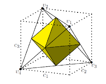
Figure 1: (Color online) Tetrahedron ${\cal T}$ with vertices $v_{1}$, $v_{2}$, $v_{3}$, and $v_{4}$ is the domain for the Bell-diagonal states. The yellow octahedron ${\cal O}$ is the set of separable states. The remaining part ${\cal T}\setminus{\cal O}$ consists of four small tetrahedra, where the entanglement is nonzero

For a clear visualization of the picture, we take slices of a three-dimensional space $(c_{1},c_{2},c_{3})$ by planes $c_{3}=const$. In this case, the cross section by the plane $c_{3}=0.7$ for Bell-diagonal states looks like shown in fig. 2.

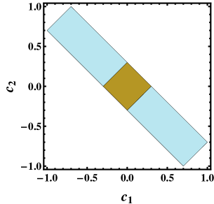
Figure 2: (Color online) Section of tetrahedron $\cal T$ and octahedron ${\cal O}$ (see Fig. 1) by plane $c_{3}=0.7$. The filled rectangle is the domain for the arguments $c_{1}$ and $c_{2}$. The blue areas of the rectangle correspond to non-zero quantum entanglement, and the square yellow area (section of octahedron ${\cal O}$) answers to the zero entanglement

Let us examine the changes that occur in the form of separability regions and in behavior of entanglement when two components of the KSEA interaction in the $\rho_{23}$-model are replaced by two analogous components of the DM interaction in the $\rho_{14}$-model: $(g_{y},g_{z})\to(\delta_{y},\delta_{z})$; in other words, when the $\rho_{23}$-model transforms into the $\rho_{14}$-model while maintaining the same strengths of interaction constants.

The domain of definitions for the nine parameters $s_{x}$, $s_{y}$, $s_{z}$, $c_{1}$, $c_{2}$, $c_{3}$, $g_{x}$, $\delta_{y}$, and $\delta_{z}$ of the $\rho_{14}$ state in its quasidiagonal form is defined by the inequalities on the main minors: by four conditions for the minors of first order which coincide with (4) and hence with the rectangle domain for the Bell-diagonal states shown in Fig 2, by three conditions for the minors of second order

$$(1+c_{1}+c_{2}-c_{3})(1+c_{1}-c_{2}+c_{3})-4(s_{x}^{2}+g_{x}^{2})\geq 0,$$

$$(1-c_{1}-c_{2}-c_{3})(1+c_{1}-c_{2}+c_{3})-4(s_{y}^{2}+\delta_{y}^{2})\geq 0,$$ (67)

$$(1-c_{1}-c_{2}-c_{3})(1+c_{1}+c_{2}-c_{3})-4(s_{z}^{2}+\delta_{z}^{2})\geq 0,$$

and by one condition for the minor of third order

$$(1-c_{1}-c_{2}-c_{3})(1+c_{1}+c_{2}-c_{3})(1+c_{1}-c_{2}+c_{3})$$

$$-4[(1-c_{1}-c_{2}-c_{3})(s_{x}^{2}+g_{x}^{2})+(1+c_{1}+c_{2}-c_{3})(s_{y}^{2}+\delta_{y}^{2})$$ (68)

$$+(1+c_{1}-c_{2}+c_{3})(s_{z}^{2}+\delta_{z}^{2})]-16(s_{x}s_{y}\delta_{z}+g_{x}s_{y}s_{z}+g_{x}\delta_{y}\delta_{z}-s_{x}\delta_{y}s_{z})\geq 0.$$

If the parameters $s_{x}$, $s_{y}$, $s_{z}$, $g_{x}$, $g_{y}$, $g_{z}$, $\delta_{x}$, $\delta_{y}$, and $\delta_{z}$ begin to change, then the tetrahedron $\cal T$ and region ${\cal O}$ will deform. We found the region of separable states using the positive partial transpose (PPT) criterion (the Peres-Horodecki criterion) HH96 ; P96 ; HHHH09 . For this, an equation $\lambda_{min}=0$ was numerically solved, where $\lambda_{min}$ is the lowest eigenvalue of the partially transposed density matrix.

Figure 3 shows how the domains and separability regions change when two components of KSEA interaction replaced by analogous components of DM interaction. It is seen that the structure of regions modifies very significantly.

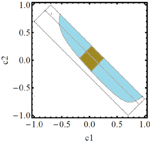
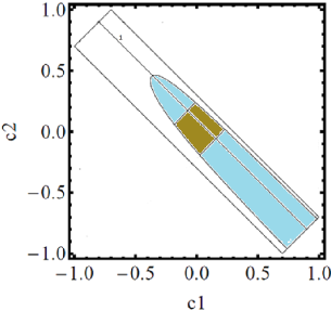
Figure 3: (Color online) Phase diagrams for the states $\rho_{23}$ (left) and $\rho_{14}$ (right) by $c_{3}=0.7$, $s_{x}=0.15$, $s_{y}=s_{z}=0$, $g_{x}=0.16$, $g_{y}=\delta_{y}=0.1$, and $g_{z}=\delta_{z}=0.04$. The filled parts of rectangles are the domains of definition. The blue areas correspond to non-zero quantum entanglement while the yellow ones to zero entanglement. Straight lines 1 are the paths $c_{2}=-c_{1}+0.1$ along which the quantum entanglement is evaluated

The behavior of quantum entanglement in both cases under discussion is presented in Fig. 4.

Figure 4: Quantum concurrence $C$ vs $c_{1}$ along the path $c_{2}=-c_{1}+0.1$ by $c_{3}=0.7$, $s_{x}=0.15$, $s_{y}=s_{z}=0$, $g_{x}=0.16$, $g_{y}=\delta_{y}=0.1$, and $g_{z}=\delta_{z}=0.04$. The dotted line corresponds to the purely KSEA interactions while the solid curve corresponds to the replacement $g_{y}$ and $g_{z}$ components by the $\delta_{y}$ and $\delta_{z}$ ones with the same strengths

We observe that the behavior of quantum entanglements in both cases, on the contrary, changes little on the whole. When the parameter $c_{1}$ begins to increase, the entanglements first decrease monotonously (see Fig. 4). At $c_{1}\approx-0.06$, the sudden death of entanglement happens and the concurrence curve has a fracture. The systems then go through the death zone where entanglement absent. However, when the control parameter $c_{1}$ reaches the critical value $c_{1}\approx 0.16$, the entanglements reincarnate and start to grow as shown in Fig. 4.

Notice the following. If the phase diagram is known, the schemes for paths can be chosen so to avoid sudden death of entanglement or, conversely, to kill him, if required (e.g., for switches of quantum entanglement).

5.2 Two-qubit states as reduced density matrices of many-body systems

If there is a $N$-particle system in the state $\rho_{N}$, one can obtain two-particle correlations between arbitrary two particles $i$ and $j$ using the reduced density matrix

$$\rho_{ij}={\rm tr}_{\{1,2,\ldots,N\}\setminus\{ij\}}\rho_{N}.$$ (69)

This circumstance makes it important to search for various families of two-site quantum states for which quantum correlations can be estimated XZYL08 .

It is known CW01 ; W02 ; ON02 ; GMPPR20 that the two-qubit reduced density matrix of one-dimensional XY chain has block-diagonal or X structures. Further, it was shown in FKY12 that the reduced density matrix of the nuclear spin pairs in a gas of $N$ molecules or atoms (for example, ${}^{129}{\rm Xe}$) in closed nanopore which is in a strong magnetic field has the CS structure. All these quantum states are part of a collection of fifteen quantum states that was recently described in Ref. Y20 .

Consider now $N$-qubit system which is symmetric under any permutations of the particles, i.e., under transformations of the symmetric group $S_{N}$. A large number of experimentally relevant multi-atom states exhibit such a symmetry. The symmetric $N$-qubit quantum state up to terms of second order can be written as

$$\rho_{N}^{sym}=\frac{1}{2^{N}}\biggl{[}1+\sum_{\alpha=x,y,z}s_{\alpha}\sum_{i=1}^{N}\sigma_{i}^{\alpha}+\sum_{\alpha,\beta=x,y,z}t_{\alpha\beta}\sum_{i<j}\sigma_{i}^{\alpha}\sigma_{j}^{\beta}+O(\sigma\sigma\sigma)\biggr{]},$$ (70)

where $s_{\alpha}$ are the components of average normalized spins of the qubits ($s_{\alpha}=\langle\sigma_{i}^{\alpha}\rangle$, $\forall i=1,\ldots,N$) and $t_{\alpha\beta}=t_{\beta\alpha}$ are the elements of the real, symmetric two-qubit correlation matrix that, without loss of generality, can be written as

$$\hat{t}=\left(\begin{array}[]{ccc}c_{1}&g_{z}&g_{y}\\ g_{z}&c_{2}&g_{x}\\ g_{y}&g_{x}&c_{3}\end{array}\right).$$ (71)

Then the reduced density matrix for a pair of qubits is written as

$$\rho_{2}^{sym}={\rm tr}_{\{3,\ldots,N\}}\rho_{N}^{sym}=\frac{1}{4}[1+{\bf s}(\vec{\sigma}_{1}+\vec{\sigma}_{2})+\vec{\sigma}_{1}\cdot\hat{t}\cdot\vec{\sigma}_{2}]$$ (72)

which exactly coincides with the density matrix $\rho_{23}$ given by Eq. (3.3). This is not surprising, because the expansion of the operator $P_{23}$ in spin Pauli matrices has the form

$$P_{23}\equiv\left(\begin{array}[]{rrrr}1&.&.&.\\ .&.&1&.\\ .&1&.&.\\ .&.&.&1\end{array}\right)=\frac{1}{2}(1+\vec{\sigma}_{1}\vec{\sigma}_{2}).$$ (73)

The right hand side of this equality represents the well-known Dirac spin exchange operator D29 ; D30 . Hence, the two-qubit reduced density matrix of symmetric state has the structure that defined by Eq. (31). This result was first established in WM02 (see also WS03 ; V06 ; KD19 ). In our paper we generalized these calculations, because we obtained an analytical formula for the pair entanglement that is suitable for the multi-qubit symmetric systems.

6 Concluding remarks and outlook

In this paper, we have found the class of four quantum states for the two-qubit Heisenberg model in an external magnetic field and with multiple components of both antisymmetric Dzyaloshinsky-Moriya and symmetric Kaplan-Shekhtman-Entin-Wohlman-Aharony interactions. The states are collected in Table 2. Then we have derived closed analytical formulas for the quantum entanglement of the found states. Thus, an assortment of families of quantum states for which quantum correlations can be obtained in closed analytical forms is extended.

Moreover, we have investigated the effect of DM-KSEA interactions on the phase diagrams of entangled-disentangled states and on the behavior of quantum entanglement. Two-qubit quantum states, for which it is possible to get explicit expressions for the quantum correlations, are important both in themselves and as reduced density matrices of many-particle systems.

Acknowledgment This work was performed as a part of the the program CITIS # AAAA-A19-119071190017-7.

References

• (1) Nielsen, M.A., Chung, I.L.: Quantum Computation and Quantum Information. Cambridge University Press, Cambridge (2000).
• (2) Valiev, K.A., Kokin, A.A.: Quantum Computers: Hops and Reality. Research Center “Regular and Chaotic Dynamics”, Moscow and Izhevsk (2002) [in Russian]
• (3) Valiev, K.A.: Quantum computers and quantum computations. Usp. Fiz. Nauk 175, 3 (2005) [in Russian]; Phys. Usp. 48, 1 (2005) [in English]
• (4) Kendon, V.M, Munro, W.J.: Entanglement and its role in Shor’s algorithm. Quantum Inf. Comput. 6, 630 (2006)
• (5) Ekert, A.K.: Quantum cryptography based on Bell’s theorem. Phys. Rev. Lett. 67, 661 (1991)
• (6) Wootters, W.K.: Quantum entanglement as a quantifiable resource. Phil. Trans. R. Soc. Lond. A 356, 1717 (1998)
• (7) Gisin, N, Ribordy, G, Tittel, W., Zbinden, H.: Quantum cryptography. Rev. Mod. Phys. 74, 145 (2002)
• (8) Yin, J., Li, Y.-H., Liao, S.-K., Yang, M., Cao, Y., Zhang, L., Ren, J.-G., Cai, W.-Q., Liu, W.-Y., Li, S.-L., Shu, R., Huang, Y.-M., Deng, L., Li, L., Zhang, Q., Liu, N.-L., Chen, Y.-A., Lu, C.-Y., Wang, X.-B., Xu, F., Wang, J.-Y., Peng, C.-Z., Ekert, A.K., Pan, J.-W.: Entanglement-based secure quantum cryptography over 1,120 kilometres. Nature 582, 501 (2020)
• (9) Pezzè, L., Smerzi, A., Oberthaler, M.K., Schmied, R., Treutlein, P.: Quantum metrology with nonclassical states of atomic ensembles. Rev. Mod. Phys. 90, 035005 (2018)
• (10) Degen, C. L., Reinhard, V, Cappellaro, P.: Quantum sensing. Rev. Mod. Phys. 89, 035002 (2017)
• (11) Pirandola, S., Bardhan, B.R., Gehring, T., Weedbrook, C., Lloyd, S.: Advances in photonic quantum sensing. Nat. Photon. 12, 724 (2018)
• (12) Lugiato, L. A.; Gatti, A.; Brambilla, E.: Quantum imaging. J. Opt. B: Quantum Semiclass. Opt. 4, S176 (2002)
• (13) Zheltikov, A.M., Scully, M.O.: Photon entanglement for life-science imaging: Rethinking the limits of the possible. Uspekhi Fiz. Nauk 190, 749 (2020) [in Russian]; Phys. Usp. 63, 698 (2020) [in English]
• (14) Feynman, R.P.: Simulating physics with computers. Int. J. Theor. Phys. 21, 467 (1982)
• (15) Lloyd, S.: Universal quantum simulators. Science 273, 1073 (1996)
• (16) Johnson, T.H., Clark, S.R., Jaksch, D. What is a quantum simulator?. EPJ Quantum Technol. 1, 10 (2014)
• (17) Altman, E., Brown, K.R., Carleo, G. et al.: Quantum simulators: Architectures and opportunities. ArXiv:1912.06938v2 [quant-ph]
• (18) Vinjanampathy, S., Anders, J.: Quantum thermodynamics. Contemp. Phys. 57, 545 (2016)
• (19) Binder, F., Correa, L.A., Gogolin, C., Anders, J., Adesso, G. (Eds.): Thermodynamics in the Quantum Regime. Springer, Berlin (2018)
• (20) Deffner, S., Campbell, S.: Quantum Thermodynamics: An introduction to the Thermodynamics of Quantum Information. Morgan and Claypool, San Rafael (2019)
• (21) Ono, K., Shevchenko, S.N., Mori, T., Moriyama, S., Nori, F.: Analog of a quantum heat engine using a single-spin qubit. Phys. Rev. Lett. 125, 166802 (2020)
• (22) Scully, M.O., Zubairy, M.S., Agarwal, G.S., Walther, H.: Extracting work from a single heat bath via vanishing quantum coherence. Science 299, 862 (2003)
• (23) Gyftopoulos, E.P.: Quantum coherence engines. Arxiv:0706.2947v1 [quant-ph]
• (24) Yi, J., Talkner, P., Kim, Y.W.: Single-temperature quantum engine without feedback control. Phys. Rev. E 96, 022108 (2017)
• (25) Barrios, G.A., Albarrán-Arriagada, F., Cárdenas-López, F.A., Romero, G., Retamal, J.C.: Role of quantum correlations in light-matter quantum heat engines. Phys. Rev. A 96, 052119 (2017)
• (26) de Assis, R.J., de Mendonca, T.M., Villas-Boas, C.J., de Souza, A.M., Sarthour, R.S., Oliveira, I.S., de Almeida, N.G.: Efficiency of a quantum Otto heat engine operating under a reservoir at effective negative temperatures. Phys. Rev. Lett. 122, 240602 (2019)
• (27) Cakmak, S., Candır, M., Altintas, F.: Construction of a quantum Carnot heat engine cycle. Quantum Inf. Process. 19: 314 (2020)
• (28) Lieb, E.H., Yngvason, J.: The physics and mathematics of the second law of thermodynamics. Phys. Rep. 310, 1 (1999)
• (29) ${\rm\acute{C}}$wikliński, P., Studziński, M., Horodecki, M., Oppenheim, J.: Limitations on the evolution of quantum coherences: Towards fully quantum second laws of thermodynamics. Phys. Rev. Lett. 115, 210403 (2015)
• (30) Kirsanov, N.S., Lebedev, A.V., Suslov, .V.M., Vinokur, V.M., Blatter, G., Lesovik, G.B.: Entropy dynamics in the system of interacting qubits. J. Russ. Laser Res., 39, 120 (2018)
• (31) Bera, M.L., Lewenstein, M., Bera, M.N.: The second laws for quantum and nano-scale heat engines. ArXiv:1911.07003v1 [quant-ph]
• (32) Bennett, C.H., Bernstein, H.J., Popescu,  S., Schumacher, B.: Concentrating partial entanglement by local operations. Phys. Rev. A 53, 2046 (1996)
• (33) Bennett, C.H., DiVincenzo, D.P., Smolin, J.A., Wootters, W.K.: Mixed-state entanglement and quantum error correction. Phys. Rev. A 54, 3824 (1996)
• (34) Wootters, W.K.: Entanglement of formation of an arbitrary state of two qubits. Phys. Rev. Lett. 80, 2245 (1998)
• (35) Hill, S., Wootters, W.K.: Entanglement of a pair of quantum bits. Phys. Rev. Lett. 78, 5022 (1997)
• (36) O’Connor, K.M.,Wootters, W.K.: Entangled rings. Phys. Rev. A 63, 052302 (2001)
• (37) Yu, T., Eberly, J.H.: Evolution from entanglement to decoherence of bipartite mixed “X” states. Quantum Inf. Comput. 7, 459 (2007)
• (38) Fel’dman, E.B., Kuznetsova, E.I., Yurishchev, M.A.: Quantum correlations in a system of nuclear $s=1/2$ spins in a strong magnetic field. J. Phys. A: Math. Theor. 45, 475304 (2012)
• (39) Weaver, J.R.: Centrosymmetric (cross-symmetric) matrices, their basic properties, eigenvalues, and eigenvectors. Am. Math. Mon. 92, 711(1985)
• (40) Ikramov, Kh.D.: The monotonicity of the eigenvalues of doubly symmetric matrices. Zh. Vychisl. Mat. Mat. Fiz. 33, 620 (1993) [in Russian]; Comput. Math. Math. Phys. 33, 561 (1993) [in English]
• (41) Yurischev, M.A.: On the quantum correlations in two-qubit XYZ spin chains with Dzyaloshinsky-Moriya and Kaplan-Shekhtman-Entin-Wohlman-Aharony interactions. Quantum Inf. Process. 19:336 (2020)
• (42) Nielsen, M.A.: Quantum information theory. PhD Dissertation, The University of New Mexico (1998); arXiv: quant-ph/0011036
• (43) Arnesen, M.C., Bose, S., Vedral, V.: Natural thermal and magnetic entanglement in the 1D Heisenberg model. Phys. Rev. Lett. 87, 017901 (2001)
• (44) Yu, T., Eberly, J.H.: Finite-time disentanglement via spontaneous emission. Phys. Rev. Lett. 93, 140404 (2004)
• (45) Yu, T., Eberly, J.H.: Sudden death of entanglement: Classical noise effects. Opt. Commun. 264, 393 (2006)
• (46) Yu, T., Eberly, J.H.: Sudden death of entanglement. Science 323, 598 (2009)
• (47) Ficek, Z., Tanaś, R.: Sudden birth and sudden death of entanglement. J. Comput. Methods Sci. Eng. 10, 265 (2010)
• (48) Wang, F., Hou, P.-Y., Huang, Y.-Y., Zhang, W.-G., Ouyang, X.-L., Wang, X., Huang, X.-Z., Zhang, H.-L., He, L., Chang, X.-Y., Duan, L.-M.: Observation of entanglement sudden death and rebirth by controlling a solid-state spin bath. Phys. Rev. B 98, 064306 (2018)
• (49) Sharma, K.K., Gerdt, V.P.: Entanglement sudden death and birth effects in two qubits maximally entangled mixed states under quantum channels. Int. J. Theor. Phys. 59, 403 (2020)
• (50) Landau, L.D., Lifshitz, E.M.: Quantum Mechanics. Non-relativistic Theory. Fizmatlit, Moscow (2005) [in Russian]; Pergamon, Oxford (1965) [in English]
• (51) Hamermesh, M.: Group Theory and Its Application to Physical Problems. Addison-Wesley, Massachusetts (1962)
• (52) Park, D.: Thermal entanglement and thermal discord in two-qubit Heisenberg XYZ chain with Dzyaloshinskii-Moriya interactions. Quantum Inf. Process. 18:172 (2019)
• (53) Korn, G.A., Korn, T.M.: Mathematical Handbook for Scientists and Engineers. Definitions, Theorems, and Formulas for Reference and Review. Dover (Press), Mineola, New York (2000)
• (54) Madelung, E.: Die mathematischen Hilfsmittel des Physikers. Springer Verlag, Berlin (1957)
• (55) Horodecki, R., Horodecki, M.: Information-theoretic aspects of inseparability of mixed states. Phys. Rev. A 54, 1838 (1996)
• (56) Peres, A.: Separability criterion for density matrices. Phys. Rev. Lett. 77, 1413 (1996)
• (57) Horodecki, R., Horodecki, P., Horodecki, M., Horodecki, K.: Quantum entanglement. Rev. Mod. Phys. 81, 865 (2009)
• (58) Xi, X.-Q., Zhang, T., Yue, R.-H., Liu, W.-M.: Pairwise entanglement and local polarization of Heisenberg model. Sci. China G: Phys. Mech. Astron. 51, 1515 (2008)
• (59) Wang, X.: Thermal and ground-state entanglement in Heisenberg XX qubit rings. Phys. Rev. A 66, 034302 (2002)
• (60) Osborne, T.J., Nielsen, M.A.: Entanglement in simple quantum phase transition. Phys. Rev. A 66, 032110 (2002)
• (61) Gombar, S., Mali, P., Panti$\rm\acute{c}$, M., Pavkov-Hrvojevi$\rm\acute{c}$, M., Rado$\rm\check{s}$evi$\rm\acute{c}$, S.: Correlation between quantum entanglement and quantum coherence in the case of XY spin chains with the Dzyaloshinskii-Moriya interaction. ZhETF 158, 228 (2020) [in Russian]; JETP 131, 209 (2020) [in English]
• (62) Dirac, P.A.M.: Quantum mechanics of many-electron systems. Proc. Roy. Soc. (London) A 123, 714 (1929)
• (63) Dirac, P.A.M.: The Principles of Quantum Mechanics. Clarendon Press, Oxford (1930)
• (64) Wang, X., M$\rm\phi$lmer, K.: Pairwise entanglement in symmetric multi-qubit systems. Eur. Phys. J. D 18, 385 (2002)
• (65) Wang, X., Sanders, B.C.: Spin squeezing and pairwise entanglement for symmetric multiqubit states. Phys. Rev. A 68, 012101 (2003)
• (66) Vidal, J.: Concurrence in collective models. Phys. Rev. A 73, 062318 (2006)
• (67) Khedif, Y., Daoud, M.: Pairwise nonclassical correlations for superposition of Dicke states via local quantum uncertainty and trace distance discord. Quantum Inf. Process. 18:45 (2019)