Laplacian-P-splines for Bayesian
            inference in the mixture cure model

Abstract

The mixture cure model for analyzing survival data is characterized by the assumption that the population under study is divided into a group of subjects who will experience the event of interest over some finite time horizon and another group of cured subjects who will never experience the event irrespective of the duration of follow-up. When using the Bayesian paradigm for inference in survival models with a cure fraction, it is common practice to rely on Markov chain Monte Carlo (MCMC) methods to sample from posterior distributions. Although computationally feasible, the iterative nature of MCMC often implies long sampling times to explore the target space with chains that may suffer from slow convergence and poor mixing. Furthermore, extra efforts have to be invested in diagnostic checks to monitor the reliability of the generated posterior samples. An alternative strategy for fast and flexible sampling-free Bayesian inference in the mixture cure model is suggested in this paper by combining Laplace approximations and penalized B-splines. A logistic regression model is assumed for the cure proportion and a Cox proportional hazards model with a P-spline approximated baseline hazard is used to specify the conditional survival function of susceptible subjects. Laplace approximations to the conditional latent vector are based on analytical formulas for the gradient and Hessian of the log-likelihood, resulting in a substantial speed-up in approximating posterior distributions. The spline specification yields smooth estimates of survival curves and functions of latent variables together with their associated credible interval are estimated in seconds. The statistical performance and computational efficiency of the proposed Laplacian-P-splines mixture cure (LPSMC) model is assessed in a simulation study. Results show that LPSMC is an appealing alternative to classic MCMC for approximate Bayesian inference in standard mixture cure models. Finally, the novel LPSMC approach is illustrated on three applications involving real survival data.

Keywords: Mixture cure model, Laplace approximation, P-splines, Approximate Bayesian inference, Survival analysis.

1 Introduction

Survival analysis is a challenging, yet very attractive area of statistical science that is devoted to the study of time-to-event data. Standard models for survival data typically leave no room for the existence of a cure fraction such that it is implicitly assumed that all subjects of the population under study will experience the event of interest as time unfolds for a sufficiently long period. Technological breakthroughs in medicine during the last decades, especially in cancer research, have led to the development of promising new treatments and therapies so that many diseases previously considered fatal can now be cured. This phenomenon has triggered the necessity to develop models that allow for long-term survivors and gave birth to cure models. A recent complete textbook treatment on cure models is proposed by Peng and Yu (2020) and an enriching literature review on cure regression models has been written by Amico and Van Keilegom (2018). Among the large family of cure models that have emerged, the mixture cure model driven by the seminal work of Boag (1949); Berkson and Gage (1952); Haybittle (1965) and later refined by Farewell (1977a, 1982) is probably the most prominent as its mathematical formulation allows for a clear and interpretable separation of the population in two categories, namely cured subjects and susceptible subjects who are at risk of experiencing the event of interest.
Let $T\in[0,+\infty)$ be a continuous random variable representing the survival time. Existence of a cure proportion in the population under study is made possible by allowing the event $\{T=+\infty\}$ to arise with positive probability. To include covariate information, denote by $\boldsymbol{X}$ and $\boldsymbol{Z}$ random covariate vectors (with continuous and/or discrete entries) that belong to covariate spaces $\mathcal{X}$ and $\mathcal{Z}$, respectively. In a mixture cure model, the population survival function expresses the separation between the cured and uncured subpopulations as follows:

$$S_{p}(t|\boldsymbol{x},\boldsymbol{z})=1-p(\boldsymbol{x})+p(\boldsymbol{x})S_{u}(t|\boldsymbol{z}),$$ (1)

with covariate vectors $\boldsymbol{x}=(x_{1},\dots,x_{p})^{\top}\in\mathcal{X}$ and $\boldsymbol{z}=(z_{1},\dots,z_{q})^{\top}\in\mathcal{Z}$ that can share (partially) the same components or can be entirely different. The term $p(\boldsymbol{x})$ is frequently called the “incidence” of the model and corresponds to the conditional probability of being uncured, i.e. $p(\boldsymbol{x})=P(B=1|\boldsymbol{X}=\boldsymbol{x})$ with binary variable $B=\mathbb{I}(T<+\infty)$ referring to the (unknown) susceptible status and $\mathbb{I}(\cdot)$ the indicator function, i.e. $\mathbb{I}(E)=1$ if condition $E$ is true. The term $S_{u}(t|\boldsymbol{z})$ is known as the “latency” and represents the conditional survival function of the uncured subjects $S_{u}(t|\boldsymbol{z})=P(T>t|B=1,\boldsymbol{Z}=\boldsymbol{z})$. The logistic link is commonly employed to establish a functional relationship between the probability to be uncured and the vector $\boldsymbol{x}$ (Farewell, 1977b; Ghitany et al., 1994; Taylor, 1995), so that $p(\boldsymbol{x})=\exp(\beta_{0}+\boldsymbol{x}^{\top}\boldsymbol{\beta})/(1+\exp(\beta_{0}+\boldsymbol{x}^{\top}\boldsymbol{\beta}))$, with regression coefficients $\boldsymbol{\beta}=(\beta_{1},\dots,\beta_{p})^{\top}$ and $\beta_{0}$ an intercept term. The latency part is often specified in a semiparametric fashion by using the Cox (1972) proportional hazards (PH) model (see e.g. Kuk and Chen, 1992; Peng and Dear, 2000) and implies the following form for the survival function of the susceptibles $S_{u}(t|\boldsymbol{z})=S_{0}(t)^{\exp(\boldsymbol{z}^{\top}\boldsymbol{\gamma})}$, where $\boldsymbol{\gamma}=(\gamma_{1},\dots,\gamma_{q})^{\top}$ are the regression coefficients pertaining to the latency part and $S_{0}(\cdot)$ is the baseline survival function.
The philosophy underlying Bayesian approaches considers that the model parameters are random and that their underlying uncertainty is characterized by probability distributions. After obtaining data, Bayes’ theorem acts as a mechanistic process describing how to update our knowledge and is essentially the key ingredient permitting the transition from prior to posterior beliefs. Unfortunately, the complexity of mixture cure models is such that the posterior distribution of latent variables of interest are not obtainable in closed form. An elegant stochastic method that is widely used in practice is Markov chain Monte Carlo (MCMC) as it allows to draw random samples from desired target posterior distributions and hence compute informative summary statistics. According to Greenhouse and Wasserman (1996), the first steps of Bayesian methods applied to mixture models with a cure fraction date back as far as Chen et al. (1985) to analyze cancer data. Later, Stangl (1991) and Stangl and Greenhouse (1998) used a Bayesian mixture survival model to analyze clinical trial data related to mental health. The end of 1990s saw the emergence of Bayesian approaches in the promotion time cure model (Chen et al., 1999), another family of cure models motivated by biological mechanisms that does not impose a mixture structure on the survival. Some references for Bayesian analysis in the latter model class are Yin and Ibrahim (2005), who proposed a Box-Cox based transformation on the population survival function to reach a unified family of cure rate models embedding the promotion time cure model as a special case; Bremhorst and Lambert (2016) used Bayesian P-splines with MCMC for flexible estimation in the promotion time cure model and Gressani and Lambert (2018) suggested a faster alternative based on Laplace approximations. More recent uses of Bayesian methods in mixture cure models are Yu and Tiwari (2012) in the context of grouped population-based cancer survival data or Martinez et al. (2013) who consider a parametric specification for the baseline survival of uncured subjects governed by a generalized modified Weibull distribution. In the literature of cure survival models, only scarce attempts have been initiated to propose an alternative to the deep-rooted MCMC instruments. This is especially true for mixture cure models, where to our knowledge Lázaro et al. (2020) is the only reference proposing an approximate Bayesian method based on a combination of Integrated Nested Laplace Approximations (INLA) (Rue et al., 2009) and modal Gibbs sampling (Gomez-Rubio, 2017). In this article, we propose a new approach for fast approximate Bayesian inference in the mixture cure model based on the idea of Laplacian-P-splines (Gressani and Lambert, 2018). The proposed Laplacian-P-splines mixture cure (LPSMC) model has various practical and numerical advantages that are worth mentioning. First, as opposed to Lázaro et al. (2020), our approach is completely sampling-free in the sense that estimation can be fully reached without the need of drawing samples from posterior distributions. This of course implies a huge gain from the computational side, without even mentioning the additional speed-up effect implied by the analytically available gradient and Hessian of the log-likelihood function in our Laplace approximation scheme. Second, the LPSMC approach delivers approximations to the joint posterior latent vector, while the INLA scheme concentrates on obtaining approximated versions of the marginal posterior of latent variables. A direct positive consequence is that with LPSMC, the “delta” method can be used to compute (approximate) credible intervals for functions of latent variables, such as the cure proportion or the survival function of the uncured, in virtually no time. A third beneficial argument is that the use of P-splines is particularly well adapted in a Bayesian framework and provide smooth estimates of the survival function. Finally, our approach and its associated algorithms are explicitly constructed to fit mixture cure models contrary to INLA that cannot fit such models originally (Lázaro et al., 2020).
The article is organized as follows. In Section 2, the spline specification of the log-baseline hazard is presented and the Bayesian model is formulated along with the prior assumptions. Laplace approximations to the conditional latent vector are derived and an approximate version of the posterior penalty parameter is proposed. The end of Section 2 is dedicated to the construction of approximate credible intervals for (functions of) latent variables. Section 3 aims at assessing the proposed LPSMC methodology in a numerical study with simulated data under different cure and censoring scenarios. Section 4 is dedicated to three real data applications and Section 5 concludes the article.

2 The Laplacian-P-spline mixture cure model

We consider that the survival time $T$ is accompanied by the frequently encountered feature of random right censoring. Rather than observing $T$ directly, one observes the pair $(T_{\text{obs}},\tau)$, where $T_{\text{obs}}=\min(T,C)$ is the follow-up time and $\tau=I(T\leq C)$ is the event indicator ($\tau=1$ if the event occurred and $\tau=0$ otherwise) and $C$ is a non-negative random censoring time that is assumed conditionally independent of $T$ given the covariates, i.e. $C\perp T|\boldsymbol{X},\boldsymbol{Z}$. At the sample level, $\mathcal{D}_{i}=(t_{i},\tau_{i},\boldsymbol{x}_{i},\boldsymbol{z}_{i})$ denotes the observables for the $i$th unit, with $t_{i}$ the realization of $T_{\text{obs}}$ and $\tau_{i}$ its associated event indicator. Vectors $\boldsymbol{x}_{i}$ and $\boldsymbol{z}_{i}$ represent the observed covariate values of subject $i$ and the entire information set available from data with sample size $n$ is denoted by $\mathcal{D}=\bigcup_{i=1}^{n}$.

2.1 Flexible modeling of the baseline risk function with B-splines

A flexible spline specification of the (log) baseline hazard function $h_{0}(\cdot)$ is proposed (Whittemore and Keller, 1986; Rosenberg, 1995) using a linear combination of cubic B-splines, i.e. $\log h_{0}(t)=\boldsymbol{\theta}^{\top}b(t)$, where $\boldsymbol{\theta}=(\theta_{1},\dots,\theta_{K})^{\top}$ is a $K-$dimensional vector of B-spline amplitudes and $b(\cdot)=(b_{1}(\cdot),\dots,b_{K}(\cdot))^{\top}$ is a cubic B-spline basis constructed from a grid of equally spaced knots in the closed interval $\mathcal{I}=[0,t_{u}]$, with $t_{u}$ the largest observed follow-up time. Partitioning $\mathcal{I}$ into $J$ (say 300) sections of equal length $\Delta$ with midpoint $s_{j}$, the Riemann midpoint rule is used to approximate the analytically unsolvable baseline survival function:

$$S_{0}(t) = \exp\left(-\int_{0}^{t}\exp\Big{(}\boldsymbol{\theta}^{\top}b(s)\Big{)}ds\right)$$

$$\approx \exp\left(-\sum_{j=1}^{j(t)}\exp\Big{(}\boldsymbol{\theta}^{\top}b(s_{j})\Big{)}\Delta\right),$$

where $j(t)\in\{1,\dots,J\}$ is an integer enumerating the interval that includes time point $t$.

2.2 Latent vector and priors

The latent vector of the model is $\boldsymbol{\xi}=(\boldsymbol{\theta}^{\top},\breve{\boldsymbol{\beta}}^{\top},\boldsymbol{\gamma}^{\top})^{\top}$ and contains the spline vector $\boldsymbol{\theta}$, the vector of regression coefficients belonging to the incidence part (including the intercept) $\breve{\boldsymbol{\beta}}=(\beta_{0},\boldsymbol{\beta}^{\top})^{\top}$ and the vector of remaining regression coefficients belonging to the latency part $\boldsymbol{\gamma}$, with dimension $\text{dim}(\boldsymbol{\xi})=K+(p+1)+q$. Based on the idea of Eilers and Marx (1996), we fix $K$ large enough to ensure flexible modeling of the baseline hazard curve and counterbalance the latter flexibility by imposing a discrete penalty on neighboring B-spline coefficients based on finite differences. In a Bayesian translation (Lang and Brezger, 2004), the prior distributional assumption on the B-spline vector is taken to be Gaussian $\boldsymbol{\theta}|\lambda\sim\mathcal{N}_{\text{dim}(\boldsymbol{\theta})}\big{(}0,(\lambda P)^{-1}\big{)}$, with a covariance matrix formed by the product of a roughness penalty parameter $\lambda>0$ and a penalty matrix $P=D_{r}^{\top}D_{r}+\varepsilon I_{K}$ obtained from $r$th order difference matrices $D_{r}$ of dimension $(K-r)\times K$. An $\varepsilon$-multiple of the $K-$dimensional identity matrix $I_{K}$ is added to ensure full rankedness (Lambert, 2011) with typical values for the scalar perturbation being $\varepsilon=10^{-6}$ (Eilers and Marx, 2021) or $\varepsilon=10^{-5}$ (Alston et al., 2013). Furthermore, a Gaussian prior is imposed on the remaining regression coefficients, with zero mean and small (common) precision $\zeta=10^{-6}$, resulting in the following proper (conditional) prior for the latent vector $\boldsymbol{\xi}|\lambda\sim\mathcal{N}_{\text{dim}(\boldsymbol{\xi})}(0,\Sigma_{\boldsymbol{\xi}}(\lambda))$ with covariance matrix:

$$\Sigma_{\boldsymbol{\xi}}(\lambda)=\begin{pmatrix}(\lambda P)^{-1}&0\\ 0&\zeta^{-1}I_{(p+1)+q}\end{pmatrix}.$$

The prior precision matrix of the latent vector is denoted by $Q_{\boldsymbol{\xi}}(\lambda)=\Sigma^{-1}_{\boldsymbol{\xi}}(\lambda)$. For full Bayesian treatment, we impose a Gamma prior with mean $a_{\lambda}/b_{\lambda}$ and variance $a_{\lambda}/b_{\lambda}^{2}$ on the roughness penalty parameter $\lambda\sim\mathcal{G}(a_{\lambda},b_{\lambda})$. Fixing $a_{\lambda}=1$ and $b_{\lambda}=10^{-5}$ (see e.g. Çetinyürek Yavuz and Lambert, 2011) yields a large variance and hence reflects a minimally informative prior for $\lambda$. Other prior specifications are also available (see e.g. Jullion and Lambert, 2007; Ventrucci and Rue, 2016).

2.3 Laplace approximations

In a mixture cure model, the full likelihood is given by (see e.g. Sy and Taylor, 2000):

$$\mathcal{L}(\boldsymbol{\xi};\mathcal{D})=\prod_{i=1}^{n}\Big{(}p(\boldsymbol{x}_{i})f_{u}(t_{i}|\boldsymbol{z}_{i})\Big{)}^{\tau_{i}}\Big{(}1-p(\boldsymbol{x}_{i})+p(\boldsymbol{x}_{i})S_{u}(t_{i}|\boldsymbol{z}_{i})\Big{)}^{(1-\tau_{i})},$$

where $f_{u}(t_{i}|\boldsymbol{z}_{i})=-(d/dt)S_{u}(t_{i}|\boldsymbol{z}_{i})$. Using the Cox PH model specification for the survival function of the susceptibles, one recovers:

$$f_{u}(t_{i}|\boldsymbol{z}_{i}) = -(d/dt)S_{u}(t_{i}|\boldsymbol{z}_{i})$$

$$= -(d/dt)S_{0}(t_{i})^{\exp(\boldsymbol{z}_{i}^{\top}\boldsymbol{\gamma})}$$

$$= -\exp(\boldsymbol{z}_{i}^{\top}\boldsymbol{\gamma})S_{0}(t_{i})^{\exp(\boldsymbol{z}_{i}^{\top}\boldsymbol{\gamma})-1}(d/dt)S_{0}(t_{i})$$

$$= \exp(\boldsymbol{z}_{i}^{\top}\boldsymbol{\gamma})S_{0}(t_{i})^{\exp(\boldsymbol{z}_{i}^{\top}\boldsymbol{\gamma})-1}f_{0}(t_{i})$$

$$= \exp(\boldsymbol{z}_{i}^{\top}\boldsymbol{\gamma})S_{0}(t_{i})^{\exp(\boldsymbol{z}_{i}^{\top}\boldsymbol{\gamma})-1}S_{0}(t_{i})h_{0}(t_{i})$$

$$= \exp(\boldsymbol{z}_{i}^{\top}\boldsymbol{\gamma})h_{0}(t_{i})S_{0}(t_{i})^{\exp(\boldsymbol{z}_{i}^{\top}\boldsymbol{\gamma})}.$$

It follows that the log-likelihood is:

$$\ell(\boldsymbol{\xi};\mathcal{D}): = \log\mathcal{L}(\boldsymbol{\xi};\mathcal{D})$$

$$= \sum_{i=1}^{n}\tau_{i}\Big{(}\log p(\boldsymbol{x}_{i})+\boldsymbol{z}_{i}^{\top}\boldsymbol{\gamma}+\log h_{0}(t_{i})+\exp(\boldsymbol{z}_{i}^{\top}\boldsymbol{\gamma})\log S_{0}(t_{i})\Big{)}$$

$$+(1-\tau_{i})\log\Big{(}1-p(\boldsymbol{x}_{i})+p(\boldsymbol{x}_{i})S_{0}(t_{i})^{\exp(\boldsymbol{z}_{i}^{\top}\boldsymbol{\gamma})}\Big{)}.$$

Using the B-spline approximations for the baseline quantities, we get:

$$\ell(\boldsymbol{\xi};\mathcal{D}) \approx \sum_{i=1}^{n}\tau_{i}\Bigg{(}\log p(\boldsymbol{x}_{i})+\boldsymbol{z}_{i}^{\top}\boldsymbol{\gamma}+\boldsymbol{\theta}^{\top}b(t_{i})-\exp(\boldsymbol{z}_{i}^{\top}\boldsymbol{\gamma})\sum_{j=1}^{j(t_{i})}\exp\big{(}\boldsymbol{\theta}^{\top}b(s_{j})\big{)}\Delta\Bigg{)}$$

$$+(1-\tau_{i})\log\Bigg{(}1-p(\boldsymbol{x}_{i})+p(\boldsymbol{x}_{i})\exp\Big{(}-\exp(\boldsymbol{z}_{i}^{\top}\boldsymbol{\gamma})\sum_{j=1}^{j(t_{i})}\exp\Big{(}\boldsymbol{\theta}^{\top}b(s_{j})\Big{)}\Delta\Big{)}\Bigg{)}.$$

Let us denote by $g_{i}(\boldsymbol{\xi})$ the contribution of the $i$th unit to the log-likelihood:

$$g_{i}(\boldsymbol{\xi}) = \tau_{i}\Bigg{(}\log p(\boldsymbol{x}_{i})+\boldsymbol{z}_{i}^{\top}\boldsymbol{\gamma}+\boldsymbol{\theta}^{\top}b(t_{i})-\exp(\boldsymbol{z}_{i}^{\top}\boldsymbol{\gamma})\sum_{j=1}^{j(t_{i})}\exp\big{(}\boldsymbol{\theta}^{\top}b(s_{j})\big{)}\Delta\Bigg{)}$$

$$+(1-\tau_{i})\log\Bigg{(}1-p(\boldsymbol{x}_{i})+p(\boldsymbol{x}_{i})\exp\Big{(}-\exp(\boldsymbol{z}_{i}^{\top}\boldsymbol{\gamma})\sum_{j=1}^{j(t_{i})}\exp\Big{(}\boldsymbol{\theta}^{\top}b(s_{j})\Big{)}\Delta\Big{)}\Bigg{)},$$

so that the log-likelihood can be compactly written as $\ell(\boldsymbol{\xi};\mathcal{D})\approx\sum_{i=1}^{n}g_{i}(\boldsymbol{\xi})$. Using Bayes’ theorem, the conditional posterior of the latent vector is (up to a proportionality constant):

$$p(\boldsymbol{\xi}|\lambda,\mathcal{D}) \propto \mathcal{L}(\boldsymbol{\xi};\mathcal{D})p(\boldsymbol{\xi}|\lambda)$$ (2)

$$\propto \exp\Big{(}\ell(\boldsymbol{\xi};\mathcal{D})-0.5\boldsymbol{\xi}^{\top}Q_{\boldsymbol{\xi}}(\lambda)\boldsymbol{\xi}\Big{)}$$

$$\propto \exp\left(\sum_{i=1}^{n}g_{i}(\boldsymbol{\xi})-0.5\boldsymbol{\xi}^{\top}Q_{\boldsymbol{\xi}}(\lambda)\boldsymbol{\xi}\right).$$

A second-order Taylor expansion of the log-likelihood yields a quadratic form in the latent vector $\boldsymbol{\xi}$ and hence can be used to obtain a Laplace approximation to (2) as shown in Appendix A. In what follows, we denote by $\widetilde{p}_{G}(\boldsymbol{\xi}|\lambda,\mathcal{D})=\mathcal{N}_{\text{dim}(\boldsymbol{\xi})}(\boldsymbol{\xi}^{*}(\lambda),\Sigma_{\boldsymbol{\xi}}^{*}(\lambda))$ the Laplace approximation to $p(\boldsymbol{\xi}|\lambda,\mathcal{D})$ for a given value of $\lambda$.

2.4 Approximate posterior of the penalty parameter

The conditional posterior in (2) is a function of the penalty parameter $\lambda$. In a frequentist setting, an “optimal” value for $\lambda$ is generally obtained by means of the Akaike information criterion (AIC) or (generalized) cross-validation. From a Bayesian perspective, $\lambda$ is random and its associated posterior distribution is of crucial importance for optimal smoothing. Mathematically, the posterior of $\lambda$ is given by:

$$p(\lambda|\mathcal{D})\propto\frac{\mathcal{L}(\boldsymbol{\xi};\mathcal{D})p(\boldsymbol{\xi}|\lambda)p(\lambda)}{p(\boldsymbol{\xi}|\lambda,\mathcal{D})}.$$ (3)

Using the Laplace approximation to $p(\boldsymbol{\xi}|\lambda,\mathcal{D})$ and replacing the latent vector by its modal value $\boldsymbol{\xi}^{*}(\lambda)$ from the Laplace approximation, the marginal posterior in (3) is approximated in the spirit of Tierney and Kadane (1986):

$$\widetilde{p}(\lambda|\mathcal{D}) \propto \frac{\exp(\ell(\boldsymbol{\xi};\mathcal{D}))p(\boldsymbol{\xi}|\lambda)p(\lambda)}{\widetilde{p}_{G}(\boldsymbol{\xi}|\lambda,\mathcal{D})}\Big{|}_{\boldsymbol{\xi}=\boldsymbol{\xi}^{*}(\lambda)}$$

$$\propto \sqrt{\det(Q_{\boldsymbol{\xi}}(\lambda))\det(\Sigma^{*}_{\boldsymbol{\xi}}(\lambda))}\exp\left(\sum_{i=1}^{n}g_{i}(\boldsymbol{\xi}^{*}(\lambda))-0.5\boldsymbol{\xi}^{*T}(\lambda)Q_{\boldsymbol{\xi}}(\lambda)\boldsymbol{\xi}^{*}(\lambda)\right)\lambda^{a_{\lambda}-1}\exp(-b_{\lambda}\lambda).$$

For numerical reasons it is more appropriate to work with the log transformed penalty parameter $v=\log(\lambda)$ as the latter is unbounded. Using the transformation method for random variables, one obtains the following approximated (log) posterior for $v$:

$$\log\widetilde{p}(v|\mathcal{D}) \dot{=} \sum_{i=1}^{n}g_{i}(\boldsymbol{\xi}^{*}(v))-0.5\boldsymbol{\xi}^{*T}(v)Q_{\boldsymbol{\xi}}(v)\boldsymbol{\xi}^{*}(v)+0.5(\log\det(Q_{\boldsymbol{\xi}}(v))+\log\det(\Sigma_{\boldsymbol{\xi}}^{*}(v)))$$ (4)

$$+a_{\lambda}v-b_{\lambda}\exp(v),$$

where $\dot{=}$ denotes equality up to an additive constant. Approximation (4) provides a good starting point for various strategies to explore the posterior penalty space. A possibility is to use grid-based approaches (Rue et al., 2009; Gressani and Lambert, 2018) or MCMC algorithms (Yoon and Wilson, 2011; Gressani and Lambert, 2021) as often encountered in models with a multidimensional penalty space. In latent Gaussian models, the posterior penalty typically satisfies suitable regularity conditions such as unimodality (Gómez-Rubio and Rue, 2018) and not a “too-large” deviation from Gaussianity. This suggests to use a simple and yet efficient type of bracketing algorithm to compute the (approximate) posterior mode $v^{*}$ of $\log\widetilde{p}(v|\mathcal{D})$. Starting with an arbitrarily “large” value, say $v_{0}=15$, the algorithm moves in the left direction with a fixed step size $\delta$, i.e. at the $m$th iteration $v_{m}=v_{m-1}-\delta$. Movement in the left direction continues until reaching $v_{\widetilde{m}}$, the point at which the target function starts to point downhill $\widetilde{p}(v_{\widetilde{m}}|\mathcal{D})<\widetilde{p}(v_{\widetilde{m}}+\delta|\mathcal{D})$. The approximated modal value is then $v^{*}=v_{\widetilde{m}}+\delta/2$. Figure 1 illustrates the normalized approximate posterior to $p(v|\mathcal{D})$ from a simulated example along with the modal value (dashed line) obtained with a step size $\delta=0.01$.

2.5 Approximate credible intervals

The Laplace approximation to the conditional posterior of the latent vector evaluated at the (approximated) modal posterior value $v^{*}$ (cf. Section 2.4) is denoted by $\widetilde{p}_{G}(\boldsymbol{\xi}|v^{*},\mathcal{D})=\mathcal{N}_{\text{dim}(\boldsymbol{\xi})}\big{(}\boldsymbol{\xi}^{*}(v^{*}),\Sigma_{\boldsymbol{\xi}}^{*}(v^{*})\big{)}$ and a point estimate for $\boldsymbol{\xi}$ is taken to be the mean/mode $\boldsymbol{\xi}^{*}(v^{*})$ with associated variance-covariance matrix $\Sigma_{\boldsymbol{\xi}}^{*}(v^{*})$. To ensure that the estimated baseline survival function $\widehat{S}_{0}(\cdot)$ “lands” smoothly on the horizontal asymptote at 0 near the end of the follow-up, we constrain the last B-spline coefficient by fixing $\theta_{K}=1$. A major advantage of LPSMC is that credible intervals for (differentiable functions of) latent variables can be straightforwardly obtained starting from $\widetilde{p}_{G}(\boldsymbol{\xi}|v^{*},\mathcal{D})$.

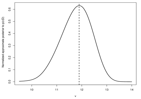
Figure 1: Approximated (normalized) posterior of the log penalty $v$. The dashed line is the modal value $v^{*}$ obtained with the bracketing algorithm using a step size $\delta=0.01$.

Credible interval for latent variables

A $(1-\alpha)\times 100\%$ (approximate) credible interval for a latent variable $\xi_{h}\in\boldsymbol{\xi}$ follows easily from the fact that the Laplace approximated posterior to $\xi_{h}$ is $\widetilde{p}_{G}(\xi_{h}|v^{*},\mathcal{D})=\mathcal{N}_{1}\big{(}\xi_{h}^{*},\sigma^{2*}_{\xi_{h}}\big{)}$, where $\xi_{h}^{*}$ is the $h$th entry of the vector $\boldsymbol{\xi}^{*}(v^{*})$ and $\sigma^{2*}_{\xi_{h}}$ is the $h$th entry on the main diagonal of $\Sigma_{\boldsymbol{\xi}}^{*}(v^{*})$. It follows that a quantile-based $(1-\alpha)\times 100\%$ credible interval for $\xi_{h}$ is:

$$\text{CI}_{\xi_{h}}=\xi_{h}^{*}\pm z_{\alpha/2}\sqrt{\sigma^{2*}_{\xi_{h}}},$$

where $z_{\alpha/2}$ is the $\alpha/2-$upper quantile of a standard normal variate.

Credible interval for the incidence $p(\boldsymbol{x})$ and cure rate $1-p(\boldsymbol{x})$

The incidence of the mixture cure model is a function of the latent vector $\breve{\boldsymbol{\beta}}$ and hence an appropriate approach to derive credible intervals for $p(\boldsymbol{x})$ is through using a “delta” method. In particular, let us consider the following differentiable function of the probability to be uncured $g(\breve{\boldsymbol{\beta}}|\boldsymbol{x})=\log\big{(}-\log p(\boldsymbol{x})\big{)}=\log\big{(}\log(1+\exp(-\beta_{0}-\boldsymbol{x}^{\top}\boldsymbol{\beta}))\big{)}$, where $\boldsymbol{x}$ is a known profile of the covariate vector. The Laplace approximated posterior to vector $\breve{\boldsymbol{\beta}}$ is known to be $\widetilde{p}_{G}(\breve{\boldsymbol{\beta}}|v^{*},\mathcal{D})=\mathcal{N}_{\text{dim}(\breve{\boldsymbol{\beta}})}\big{(}\breve{\boldsymbol{\beta}}^{*},\Sigma^{*}_{\breve{\boldsymbol{\beta}}}\big{)}$ with mean vector $\breve{\boldsymbol{\beta}}^{*}=\breve{\boldsymbol{\beta}}^{*}(v^{*})$ and covariance matrix $\Sigma^{*}_{\breve{\boldsymbol{\beta}}}=\Sigma^{*}_{\breve{\boldsymbol{\beta}}}(v^{*})$. The delta method operates via a first-order Taylor expansion of $g(\breve{\boldsymbol{\beta}}|\boldsymbol{x})$ around $\breve{\boldsymbol{\beta}}^{*}$:

$$g(\breve{\boldsymbol{\beta}}|\boldsymbol{x})\approx g(\breve{\boldsymbol{\beta}}^{*}|\boldsymbol{x})+(\breve{\boldsymbol{\beta}}-\breve{\boldsymbol{\beta}}^{*})^{\top}\nabla g(\breve{\boldsymbol{\beta}}|\boldsymbol{x})\big{|}_{\breve{\boldsymbol{\beta}}=\breve{\boldsymbol{\beta}}^{*}},$$ (5)

with gradient:

$$\nabla g(\breve{\boldsymbol{\beta}}|\boldsymbol{x}) = \left(\frac{\partial g(\breve{\boldsymbol{\beta}}|\boldsymbol{x})}{\partial\beta_{0}},\dots,\frac{\partial g(\breve{\boldsymbol{\beta}}|\boldsymbol{x})}{\partial\beta_{p}}\right)^{\top}$$

$$= \frac{-(1-p(\boldsymbol{x}))}{\log\big{(}1+\exp(-\beta_{0}-\boldsymbol{x}^{\top}\boldsymbol{\beta})\big{)}}\ (1,\boldsymbol{x}^{\top})^{\top}.$$

Note that $g(\breve{\boldsymbol{\beta}}|\boldsymbol{x})$ in (5) is still Gaussian as it is a linear combination of a random vector $\breve{\boldsymbol{\beta}}$ that is a posteriori (approximately) Gaussian due to the Laplace approximation with mean $\mathbb{E}(g(\breve{\boldsymbol{\beta}}|\boldsymbol{x}))\approx g(\breve{\boldsymbol{\beta}}^{*}|\boldsymbol{x})$ and covariance matrix $\mathbb{V}(g(\breve{\boldsymbol{\beta}}|\boldsymbol{x}))\approx\nabla^{\top}g(\breve{\boldsymbol{\beta}}|\boldsymbol{x})|_{\breve{\boldsymbol{\beta}}=\breve{\boldsymbol{\beta}}^{*}}\Sigma^{*}_{\breve{\boldsymbol{\beta}}}\nabla g(\breve{\boldsymbol{\beta}}|\boldsymbol{x})|_{\breve{\boldsymbol{\beta}}=\breve{\boldsymbol{\beta}}^{*}}$. This suggests to write the approximated posterior of $g(\breve{\boldsymbol{\beta}}|\boldsymbol{x})$ as:

$$\big{(}g(\breve{\boldsymbol{\beta}}|\boldsymbol{x})|\mathcal{D}\big{)}\sim\mathcal{N}_{1}\left(g(\breve{\boldsymbol{\beta}}^{*}|\boldsymbol{x}),\nabla^{\top}g(\breve{\boldsymbol{\beta}}|\boldsymbol{x})|_{\breve{\boldsymbol{\beta}}=\breve{\boldsymbol{\beta}}^{*}}\Sigma^{*}_{\breve{\boldsymbol{\beta}}}\nabla g(\breve{\boldsymbol{\beta}}|\boldsymbol{x})|_{\breve{\boldsymbol{\beta}}=\breve{\boldsymbol{\beta}}^{*}}\right)$$

and so an approximate quantile-based $(1-\alpha)\times 100\%$ credible interval for $g(\breve{\boldsymbol{\beta}}|\boldsymbol{x})$ is:

$$CI_{g(\breve{\boldsymbol{\beta}}|\boldsymbol{x})}=g(\breve{\boldsymbol{\beta}}^{*}|\boldsymbol{x})\pm z_{\alpha/2}\sqrt{\nabla^{\top}g(\breve{\boldsymbol{\beta}}|\boldsymbol{x})|_{\breve{\boldsymbol{\beta}}=\breve{\boldsymbol{\beta}}^{*}}\Sigma^{*}_{\breve{\boldsymbol{\beta}}}\nabla g(\breve{\boldsymbol{\beta}}|\boldsymbol{x})|_{\breve{\boldsymbol{\beta}}=\breve{\boldsymbol{\beta}}^{*}}}.$$ (6)

Multiplying the values in the interval (6) by $\exp(-\exp(\cdot))$ gives us the desired credible interval for the incidence $p(\boldsymbol{x})$. If a credible interval for the cure rate $1-p(\boldsymbol{x})$ is required, simply use the transformation $g(\breve{\boldsymbol{\beta}}|\boldsymbol{x})=\log\big{(}-\log(1-p(\boldsymbol{x}))\big{)}=\log\big{(}\log(1+\exp(\beta_{0}+\boldsymbol{x}^{\top}\boldsymbol{\beta}))\big{)}$ with gradient $\nabla g(\breve{\boldsymbol{\beta}}|\boldsymbol{x})=\Big{(}p(\boldsymbol{x})/\log(1+\exp(\beta_{0}+\boldsymbol{x}^{\top}\boldsymbol{\beta}))\Big{)}(1,\boldsymbol{x}^{\top})^{\top}$.

Credible interval for $S_{0}(\cdot)$ and $S_{u}(\cdot|\boldsymbol{z})$

Let us denote by $t_{q}$ the $q$th quantile of the distribution of the survival time $T$ at baseline by $t_{q}=\inf\{t|S_{0}(t)\leq 1-q\}$. The “delta” method can also be used to compute an approximate credible interval for $S_{0}(\cdot)$ at $t_{q}$ by using a $\log(-\log(\cdot))$ transformation $g(\boldsymbol{\theta}|t_{q})=\log(-\log(S_{0}(t_{q})))=\log\big{(}\sum_{j=1}^{j(t_{q})}\exp(\boldsymbol{\theta}^{\top}b(s_{j}))\Delta\big{)}$. Starting from the Laplace approximated posterior $\widetilde{p}_{G}(\boldsymbol{\theta}^{*}|v^{*},\mathcal{D})=\mathcal{N}_{\text{dim}(\boldsymbol{\theta})}(\boldsymbol{\theta}^{*},\Sigma_{\boldsymbol{\theta}}^{*})$, one can show that the resulting credible interval for $g(\boldsymbol{\theta}|t_{q})$ is:

$$CI_{g(\boldsymbol{\theta}|t_{q})}=g(\boldsymbol{\theta}^{*}|t_{q})\pm z_{\alpha/2}\sqrt{\nabla^{\top}g(\boldsymbol{\theta}|t_{q})|_{\boldsymbol{\theta}=\boldsymbol{\theta}^{*}}\Sigma^{*}_{\boldsymbol{\theta}}\nabla g(\boldsymbol{\theta}|t_{q})|_{\boldsymbol{\theta}=\boldsymbol{\theta}^{*}}},$$ (7)

where $\nabla g(\boldsymbol{\theta}|t_{q})|_{\boldsymbol{\theta}=\boldsymbol{\theta}^{*}}$ is the gradient of $g(\boldsymbol{\theta}|t_{q})$ with respect to $\boldsymbol{\theta}$ evaluated at $\boldsymbol{\theta}^{*}$ and can be found in Gressani and Lambert (2018) Appendix C. Applying the inverse transformation $\exp(-\exp(\cdot))$ to (7) yields the desired $(1-\alpha)\times 100\%$ credible interval for $S_{0}(\cdot)$ at $t_{q}$.
The same approach is used to construct credible intervals for the survival function of the uncured $S_{u}(t|\boldsymbol{z})=S_{0}(t)^{\exp(\boldsymbol{z}^{\top}\boldsymbol{\gamma})}$ at $t_{q}=\inf\{t|S_{u}(t|\boldsymbol{z})\leq 1-q\}$ for a given covariate profile $\boldsymbol{z}$. Applying the $\log(-\log(\cdot))$ transform yields $g(\boldsymbol{\theta},\boldsymbol{\gamma}|t_{q},\boldsymbol{z})=\boldsymbol{z}^{\top}\boldsymbol{\gamma}+\log\big{(}\sum_{j=1}^{j(t_{q})}\exp(\boldsymbol{\theta}^{\top}b(s_{j}))\Delta\big{)}$ with gradient:

$$\nabla g(\boldsymbol{\theta},\boldsymbol{\gamma}|t_{q},\boldsymbol{z}) = \left(\frac{\partial g(\boldsymbol{\theta},\boldsymbol{\gamma}|t_{q},\boldsymbol{z})}{\partial\theta_{1}},\dots,\frac{\partial g(\boldsymbol{\theta},\boldsymbol{\gamma}|t_{q},\boldsymbol{z})}{\partial\theta_{K}},\frac{\partial g(\boldsymbol{\theta},\boldsymbol{\gamma}|t_{q},\boldsymbol{z})}{\partial\gamma_{1}},\dots,\frac{\partial g(\boldsymbol{\theta},\boldsymbol{\gamma}|t_{q},\boldsymbol{z})}{\partial\gamma_{q}}\right)^{\top}$$

$$= \begin{pmatrix}\left(\sum_{j=1}^{j(t_{q})}\exp(\boldsymbol{\theta}^{\top}b(s_{j}))\Delta\right)^{-1}\sum_{j=1}^{j(t_{q})}\exp(\boldsymbol{\theta}^{\top}b(s_{j}))b_{1}(s_{j})\Delta\\ \vdots\\ \left(\sum_{j=1}^{j(t_{q})}\exp(\boldsymbol{\theta}^{\top}b(s_{j}))\Delta\right)^{-1}\sum_{j=1}^{j(t_{q})}\exp(\boldsymbol{\theta}^{\top}b(s_{j}))b_{K}(s_{j})\Delta\\ z_{1}\\ \vdots\\ z_{q}\end{pmatrix}.$$

The resulting credible interval for $g(\boldsymbol{\theta},\boldsymbol{\gamma}|t_{q},\boldsymbol{z})$ is:

$$CI_{g(\boldsymbol{\theta},\boldsymbol{\gamma}|t_{q},\boldsymbol{z})}=g(\boldsymbol{\theta}^{*},\boldsymbol{\gamma}^{*}|t_{q},\boldsymbol{z})\pm z_{\alpha/2}\sqrt{\nabla^{\top}g(\boldsymbol{\theta},\boldsymbol{\gamma}|t_{q},\boldsymbol{z})|_{\boldsymbol{\theta}=\boldsymbol{\theta}^{*},\boldsymbol{\gamma}=\boldsymbol{\gamma}^{*}}\Sigma^{*}_{\boldsymbol{\theta},\boldsymbol{\gamma}}\nabla g(\boldsymbol{\theta},\boldsymbol{\gamma}|t_{q},\boldsymbol{z})|_{\boldsymbol{\theta}=\boldsymbol{\theta}^{*},\boldsymbol{\gamma}=\boldsymbol{\gamma}^{*}}},$$ (8)

where $\Sigma^{*}_{\boldsymbol{\theta},\boldsymbol{\gamma}}$ is the covariance matrix of the vector $(\boldsymbol{\theta}^{\top},\boldsymbol{\gamma}^{\top})^{\top}$ obtained from the Laplace approximation. Finally, an $\exp(-\exp(\cdot))$ transform on (8) gives a $(1-\alpha)\times 100\%$ credible interval for $S_{u}(t|\boldsymbol{z})$ at $t_{q}$ for a given covariate vector $\boldsymbol{z}$.

3 Simulation study

To measure the statistical performance of the LPSMC methodology in a mixture cure model setting, we consider a numerical study where survival data is generated according to different cure and censoring rates. Generation of survival data for the $i$th subject is as follows. The incidence part is generated from a logistic regression function with two covariates $p(\boldsymbol{X}_{i})=1/(1+\exp(-\beta_{0}-\beta_{1}X_{i1}-\beta_{2}X_{i2}))$, where $X_{i1}$ is a standard normal variate and $X_{i2}\sim\text{Bern}(0.5)$ is a Bernoulli random variable. The cure status is generated as a Bernoulli random variable with failure probability $p(\boldsymbol{X}_{i})$, i.e. $B_{i}\sim\text{Bern}(p(\boldsymbol{X}_{i}))$. Survival times $T_{i}$ for the uncured subjects ($B_{i}=1$) are obtained from a Weibull Cox proportional hazards model and are truncated at $\tau_{0}=8$. The latency is given by $S_{u}(t_{i}|\boldsymbol{Z}_{i})=\exp(-\nu t_{i}^{\varrho}\exp(\gamma_{1}Z_{i1}+\gamma_{2}Z_{i2}))$, with scale parameter $\nu=0.25$ and shape $\varrho=1.45$. The covariate vector $\boldsymbol{Z}_{i}=(Z_{i1},Z_{i2})^{\top}$ is independent of $\boldsymbol{X}_{i}$. We assume that $Z_{i1}$ follows a standard Gaussian distribution and $Z_{i2}\sim\text{Bern}(0.4)$. For the cured subject ($B_{i}=0$), the theoretically infinite survival times are replaced by a large value, say $T_{i}=20,000$. The censoring time $C_{i}$ is independent of the vector $(\boldsymbol{X}_{i}^{\top},\boldsymbol{Z}_{i}^{\top},T_{i})^{\top}$ and is generated from an exponential distribution with density function $f(c_{i})=\mu_{c}\exp(-\mu_{c}c_{i})$ truncated at $\tau_{1}=11$. We consider samples of sizes $n=300$ and $n=600$ and simulate survival data with two scenarios for the coefficients $\boldsymbol{\beta}$, $\boldsymbol{\gamma}$ and $\mu_{c}$, yielding different censoring and cure rates. In both scenarios (almost) all the observations in the plateau of the Kaplan and Meier (1958) estimator are cured, such that the simulated data are representative of the practical real case scenarios for which mixture cure models are used. Table 1 provides a summary of the two considered scenarios.
We specify $15$ cubic B-splines in the interval $[0,t_{u}]$ with upper bound fixed at $t_{u}=11$ and a third order penalty to counterbalance model flexibility. In the bracketing algorithm, we use a step size $\delta=0.2$ to compute the (approximate) modal posterior log penalty value $v^{*}$. For each scenario, we simulate $S=500$ replications and compute the bias, empirical standard error (ESE), root mean square error (RMSE) and coverage probabilities for $90\%$ and $95\%$ credible intervals.

Scenario	$\beta_{0}$	$\beta_{1}$	$\beta_{2}$	$\gamma_{1}$	$\gamma_{2}$	Cure	$\mu_{c}$	Censoring	Plateau
1	0.70	-1.15	0.95	-0.10	0.25	$28.8\%$	0.16	$48.5\%$	$9.6\%$
2	1.25	-0.75	0.45	-0.10	0.20	$21.0\%$	0.05	$29.3\%$	$14.4\%$

Table 1: Parameters for the incidence, latency and censoring rate yielding different cure and censoring levels. The last column indicates the percentage of observations in the plateau.

Results are summarized in Table 2. The bias is negligible and the ESE and RMSE decrease with larger sample size, as expected. In addition, the estimated coverage probabilities are close to their respective nominal value in all scenarios. The LPSMC methodology is extremely fast as it takes $\sim$ 0.7 seconds to fit a model with an algorithm coded in $\bf{R}$ with an Intel Xeon E-2186M processor at 2.90GHz. Figure 2 shows the estimated baseline survival curves (gray), the target (solid) and the pointwise median of the $500$ curves (dashed) for the different scenarios.
Another performance measure for the incidence of the model is obtained by computing the Average Squared Error (ASE) of $\widehat{p}(\boldsymbol{x})$ defined as $ASE(\widehat{p})=M^{-1}\sum_{m=1}^{M}\big{(}\widehat{p}(\boldsymbol{x})-p(\boldsymbol{x})\big{)}^{2}$. The latter quantity is computed on triplets of covariate values $\boldsymbol{x}_{m}=(1,x_{m1},x_{m2})^{\top}$ for $m=1,\dots,M$, where the set of couples $\{(x_{m1},x_{m2})\}_{m=1}^{M}$ equals the Cartesian product between an equidistant grid in $[-1.50,1.50]$ with step size $0.001$ (for variable $x_{1}$) and the set $\{0,1\}$ (for $x_{2}$). Boxplots for the ASE in the different scenarios are displayed in Figure 3. Coverage probability of the $90\%$ and $95\%$ (approximate) credible interval for the incidence $p(\boldsymbol{x})$ (and cure rate $1-p(\boldsymbol{x})$) at the mean covariate profile $\bar{\boldsymbol{x}}=(1,0,0.5)^{\top}$ as computed from (6) have also been measured and are close to their nominal value in all scenarios.

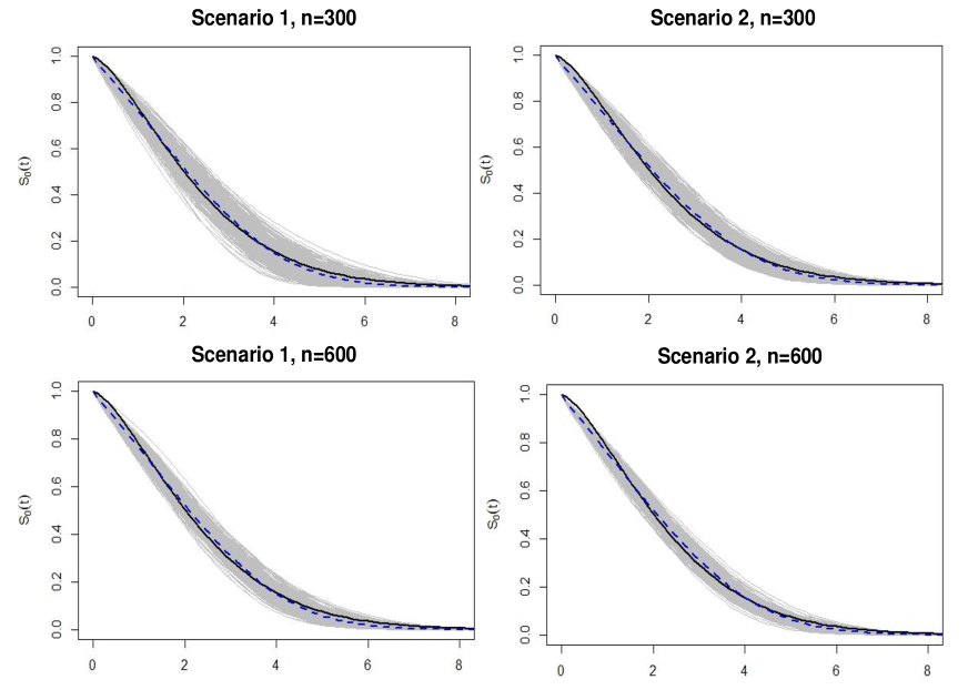
Figure 2: Estimated baseline survival curves (gray) for $S=500$ replications under different scenarios. The black curve is the target baseline and the dashed curve the pointwise median of the 500 gray curves.

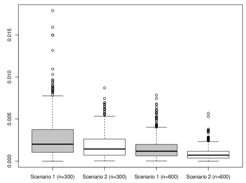
Figure 3: Boxplots of the ASE for the incidence in different scenarios.

Scenario	Parameters	Mean	Bias	ESE	RMSE	$\text{CP}_{90\%}$	$\text{CP}_{95\%}$
	$\beta_{0}=\phantom{-}0.70$	0.720	0.020	0.249	0.249	91.0	97.0
	$\beta_{1}=-1.15$	-1.180	-0.030	0.240	0.242	91.6	95.0
Scenario 1	$\beta_{2}=\phantom{-}0.95$	0.953	0.003	0.390	0.390	90.6	94.2
($n=300$)	$\gamma_{1}=-0.10$	-0.101	-0.001	0.092	0.092	89.8	94.4
	$\gamma_{2}=\phantom{-}0.25$	0.247	-0.003	0.185	0.184	89.0	96.2
	$\beta_{0}=\phantom{-}1.25$	1.277	0.027	0.228	0.229	91.4	95.8
	$\beta_{1}=-0.75$	-0.763	-0.013	0.182	0.182	91.0	95.4
Scenario 2	$\beta_{2}=\phantom{-}0.45$	0.429	-0.021	0.329	0.329	89.0	95.0
($n=300$)	$\gamma_{1}=-0.10$	-0.103	-0.003	0.074	0.074	89.2	94.4
	$\gamma_{2}=\phantom{-}0.20$	0.197	-0.003	0.151	0.150	87.4	95.0
	$\beta_{0}=\phantom{-}0.70$	0.699	-0.001	0.184	0.184	90.0	95.6
	$\beta_{1}=-1.15$	-1.150	0.000	0.166	0.166	90.4	95.2
Scenario 1	$\beta_{2}=\phantom{-}0.95$	0.948	-0.002	0.268	0.267	90.8	95.0
($n=600$)	$\gamma_{1}=-0.10$	-0.102	-0.002	0.064	0.064	89.6	95.0
	$\gamma_{2}=\phantom{-}0.25$	0.256	0.006	0.127	0.127	90.8	96.0
	$\beta_{0}=\phantom{-}1.25$	1.241	-0.009	0.160	0.160	91.2	95.8
	$\beta_{1}=-0.75$	-0.744	0.006	0.129	0.129	90.0	95.4
Scenario 2	$\beta_{2}=\phantom{-}0.45$	0.457	0.007	0.222	0.222	91.4	95.8
($n=600$)	$\gamma_{1}=-0.10$	-0.100	0.000	0.054	0.054	88.6	95.6
	$\gamma_{2}=\phantom{-}0.20$	0.200	0.000	0.105	0.105	90.6	95.2

Table 2: Numerical results for $S=500$ replications of sample size $n=300$ and $n=600$ under two different cure-censoring scenarios.

In Table 3, the performance of approximate credible intervals for the baseline survival and survival of the uncured for a mean covariate profile $\bar{\boldsymbol{z}}=(0,0.4)^{\top}$ at selected quantiles of $T$ is shown. Results are for $S=500$ replications of sample size $n=300$ with $K=30$ B-splines.

	Nominal	Scenario	$t_{0.20}$	$t_{0.30}$	$t_{0.40}$	$t_{0.50}$	$t_{0.60}$	$t_{0.70}$	$t_{0.80}$	$t_{0.90}$	$t_{0.95}$
	90	1	83.2	92.4	91.4	90.6	89.8	89.8	90.6	86.0	79.6
Baseline	95	1	91.0	95.6	95.0	94.2	93.6	93.8	94.4	93.2	88.2
$S_{0}(\cdot)$	90	2	76.0	91.2	93.0	93.4	90.6	91.0	91.2	84.4	80.0
	95	2	84.0	95.6	96.6	96.6	95.8	95.8	95.0	90.6	86.6
	90	1	81.6	93.6	93.2	89.8	89.0	88.8	89.0	90.4	83.4
Uncured	95	1	92.2	96.4	97.0	95.2	94.2	94.6	94.0	95.4	90.0
$S_{u}(\cdot|\bar{\boldsymbol{z}})$	90	2	77.4	91.8	94.2	93.4	92.0	90.6	89.8	86.0	79.4
	95	2	85.8	95.8	97.6	97.0	95.8	95.4	94.4	92.6	86.0

Table 3: Estimated coverage probability of $90\%$ and $95\%$ credible intervals for $S_{0}(\cdot)$ and $S_{u}(\cdot|\bar{\boldsymbol{z}}=(0,0.4)^{\top})$ with $S=500$ replications of sample size $n=300$ and $K=30$ B-splines.

4 Real data applications

4.1 ECOG e1684 clinical trial

We start by applying the LPSMC methodology to a well-known dataset in the cure literature and compare the estimates with the ones obtained using the benchmark smcure package (Cai et al., 2012). The data comes from the Eastern Cooperative Oncology Group (ECOG) phase III two-arm clinical trial with $n=284$ observations after removing missing data. The aim of the study was to assess whether Interferon alpha-2b (IFN) had a significant effect on relapse-free survival. There were 144 patients receiving the treatment and the remaining patients (140) belonged to the control group. The response of interest is relapse-free survival time measured in years. The following covariates enter both the incidence and latency part of the model. TRT is the binary variable indicating whether a patient received the IFN treatment ($TRT=1$) or not ($TRT=0$). Variable SEX indicates if a patient is female ($SEX=1$) or male ($SEX=0$). In total the study involves 113 women and 171 men. Finally, AGE is a continuous covariate (centered to the mean) indicating the age of patients. Figure 4, shows the Kaplan-Meier estimated survival curve for the e1684 dataset. A plateau is clearly visible indicating the potential presence of a cure fraction, so that a mixture cure model is appropriate to fit this type of data.

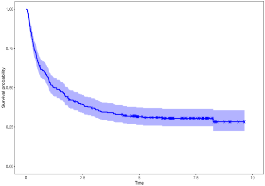
Figure 4: Kaplan-Meier estimated survival for the e1684 ECOG dataset. A cross indicates a censored observation.

Table 4 summarizes the estimation results for the e1684 dataset with LPSMC and smcure. The estimated coefficients in the two parts of the model (incidence and latency) are of similar magnitude for both approaches. However, the computational times to fit the mixture cure model drastically differ depending on the method.

Model	Parameter	Estimate	Sd	CI $90\%$
LPSMC	$\beta_{0}$ (Intercept)	1.235	0.255	[-0.817; -1.654]
(Incidence)	$\beta_{1}$ (SEX)	-0.064	0.291	[-0.542; -0.415]
	$\beta_{2}$ (TRT)	-0.572	0.289	[-1.046; -0.097]
	$\beta_{3}$ (AGE)	0.016	0.011	[-0.003; -0.035]
smcure	$\beta_{0}$ (Intercept)	1.365	0.329	[-0.823; -1.906]
(Incidence)	$\beta_{1}$ (SEX)	-0.087	0.333	[-0.634; -0.461]
	$\beta_{2}$ (TRT)	-0.588	0.343	[-1.152; -0.025]
	$\beta_{3}$ (AGE)	0.020	0.016	[-0.006; -0.047]
LPSMC	$\gamma_{1}$ (SEX)	0.096	0.177	[-0.195; -0.388]
(Latency)	$\gamma_{2}$ (TRT)	-0.131	0.179	[-0.425; -0.163]
	$\gamma_{2}$ (AGE)	-0.007	0.006	[-0.017; -0.003]
smcure	$\gamma_{1}$ (SEX)	0.099	0.175	[-0.189; -0.388]
(Latency)	$\gamma_{2}$ (TRT)	-0.154	0.177	[-0.444; -0.137]
	$\gamma_{3}$ (AGE)	-0.008	0.007	[-0.019; -0.004]

Table 4: Estimation results for the e1684 dataset with LPSMC and smcure. The first column indicates the model part, the second and third columns the parameter and its estimate. The fourth column is the (posterior) standard deviation of the estimate and the last column the $90\%$ confidence/credible interval.

It takes approximately 128 seconds to fit the model with smcure, while LPSMC takes only 1.6 seconds. This speedup factor of $\approx 80$ is mainly due to the bootstrap samples that smcure uses to compute estimates of the variance of estimated parameters. The LPSMC approach is completely sampling-free and intrinsically accounts for fast computation of credible intervals for the latent variables. Results for both smcure and LPSMC show that treatment (TRT) has a significant and positive impact on the cure probability (incidence), while IFN treatment has no significative impact in the latency part. In other words, taking AGE and SEX into account, receiving the IFN treatment decreases the probability to be susceptible but will not postpone relapse among the uncured. Similar findings are reported in Corbière and Joly (2007) and Legrand et al. (2019).

4.2 Breast cancer data

The second dataset used to illustrate the LPSMC methodology concerns $n=286$ patients with breast cancer studied in Wang et al. (2005). Survival time (in days) is defined as the distant-metastasis-free survival (DMFS), i.e. time to occurrence of distant metastases or death (whatever happens first) and the event of interest is distant-metastasis. The data is obtained from the breastCancerVDX package (Schroeder et al., 2020) on Bioconductor (https://bioconductor.org/). We consider two covariates entering simultaneously in the incidence and latency part, namely the age of patients, ranging between 26 and 83 years with a median of 52 years and the categorical variable Estrogen Receptor (ER) (with $ER=0$: if $\leq 10$ fmol per mg protein [77 patients] and $ER=1$ otherwise [209 patients]). We use $K=20$ cubic B-splines in $[0,t_{u}]$, with $t_{u}=5201$ days, the largest follow-up time. The Kaplan-Meier estimate of the data given in Figure 5 emphasizes the existence of a plateau and motivates the use of a mixture cure model.

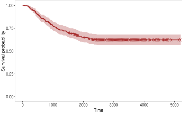
Figure 5: Kaplan-Meier estimated survival for the breast cancer data. A cross indicates a censored observation.

The estimated latent variables with LPSMC are reported in Table5. We see that AGE and ER have no significant effect on the probability of being uncured (incidence) at significance level $0.05$. However, the latter two covariates significantly affect the survival of the uncured.

Model	Parameter	Estimate	Sd	CI $95\%$
	$\beta_{0}$ (Intercept)	-0.015	0.576	[-1.143; -1.112]
(Incidence)	$\beta_{1}$ (AGE)	-0.012	0.010	[-0.031; -0.008]
	$\beta_{2}$ (ER)	0.181	0.281	[-0.369; -0.731]
(Latency)	$\gamma_{1}$ (AGE)	-0.018	0.008	[-0.034; -0.002]
	$\gamma_{2}$ (ER)	-1.063	0.243	[-1.539; -0.586]

Table 5: Estimation results for the breast cancer data with LPSMC. The first column indicates the model part, the second and third columns the parameter and its posterior (mean) estimate. The fourth column is the posterior standard deviation of the estimate and the last column the $95\%$ credible interval.

For instance, a subject that is susceptible to experience metastasis with $ER=1$ has a risk of experiencing the event that is $1/\exp(-1.063)=2.90$ times smaller than the risk with $ER=0$. In Figure 6 the estimated survival for the susceptible subjects is shown for two age categories ($30$ years and $50$ years) with $ER=1$.

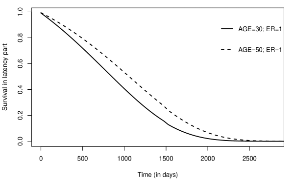
Figure 6: Estimated survival of the susceptibles for two age categories and $ER=1$.

4.3 ZNA COVID-19 data

In a third application, we use LPSMC to investigate the impact of age on survival of Covid-19 patients. The data comes from the Ziekenhuis Netwerk Antwerpen (ZNA, Belgium), a network of hospitals in the province of Antwerp. The considered dataset has $n=3258$ patients entering hospitals between March 2020 and April 2021. The follow-up time is defined as the total number of days spent in hospital and receiving COVID-19 care. The outcome of interest is in-hospital death due to Covid-19 as indicated by a binary variable (1 = Dead; 0 = Alive). Among the 3258 patients, 461 (14.15$\%$) experienced in-hospital death and the remaining 2797 (85.85$\%$) are censored due to causes unrelated to the outcome of interest (uninformative censoring). The Kaplan-Meier curve is given in Figure 7 and highlights a wide plateau around 0.52, suggesting the existence of a cure fraction and hence motivating a cure model analysis with LPSMC. The age of patients is taken as a covariate both in the incidence and latency part of the model. The mean age is 66 years and the youngest, respectively oldest patient is 1 and 103 years old. We use $K=15$ cubic B-splines between $0$ and the largest follow-up time ($t_{u}=98.88$) along with a third order penalty.

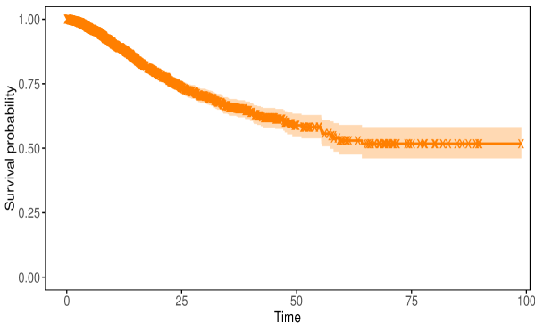
Figure 7. Kaplan-Meier estimated survival for the ZNA data. A cross indicates a censored observation.

Table 6 summarizes the estimation results for the model parameters with the LPSMC methodology. We see that AGE has a positive and significant effect in the incidence part of the model. In other words, older patients have a larger probability of being uncured and hence a smaller probability to be cured from COVID-19. The estimated cure proportion for different AGE categories is shown in Table 7. In the latency part, AGE is positive and not significant at the 0.05 level and thus there is no significant effect of AGE on the survival of uncured patients.

Model	Parameter	Estimate	Sd	CI $95\%$
	$\beta_{0}$ (Intercept)	-2.625	0.763	[-4.120; -1.130]
(Incidence)	$\beta_{1}$ (AGE)	0.031	0.010	[-0.012; -0.051]
(Latency)	$\gamma_{1}$ (AGE)	0.010	0.007	[-0.004; -0.024]

Table 6: Estimation results for the ZNA data with LPSMC. The first column indicates the model part, the second and third columns the parameter and its posterior (mean) estimate. The fourth column is the posterior standard deviation of the estimate and the last column the $95\%$ credible interval.

AGE	$1-\widehat{p}(\boldsymbol{x})$	CI $95\%$
20	0.880	[0.695; -0.956]
30	0.843	[0.669; -0.930]
50	0.741	[0.612; -0.833]
80	0.527	[0.463; -0.586]

Table 7: Estimation of the cure proportion for different age categories and associated $95\%$ approximate credible interval.

5 Conclusion

Approximate Bayesian inference methods are an interesting alternative to classic MCMC algorithms, especially when the latter require long computation times, as can be the case for models with complex likelihoods. In survival analysis, the mixture cure model is an interesting class of models that allows for the existence of a cure fraction and hence goes beyond classic proportional hazards model for which the feature of long-term survivors is absent. In this article, we propose a new approach for fast Bayesian inference in the standard mixture cure model by combining the strength of Laplace approximations to selected posterior distributions of latent variables and P-splines for flexible modeling of baseline smooth quantities. The attractiveness of the LPSMC approach lies in its completely sampling-free framework, with an analytically available gradient and Hessian of the log-likelihood that makes the approach extremely fast from a computational viewpoint. This computational advantage and the relatively straightforward possibility to derive (approximate) credible intervals for functions of latent variables makes it a promising tool for fast analysis of survival data with a cure fraction. A possible interesting extension for future research would be to generalize the LPSMC approach at the level of the incidence with alternative specifications to the standard logistic regression model. For instance, LPSMC could be extended to the single-index/Cox mixture cure model of Amico et al. (2019). Finally, Laplacian-P-splines can also be extended in cure models with frailties or in the context of competing risks survival data with a cure fraction.

Software

R code for the simulation scenarios in Section 3 and the ECOG and breast cancer data applications in Section 4 are publicly available on https://github.com/oswaldogressani/LPSMC.

Conflict of interest

The authors declare no conflicts of interest.

Appendix A

Recall that the contribution of the $i$th unit to the log-likelihood is given by:

$$g_{i}(\boldsymbol{\xi}) = \tau_{i}\Bigg{(}\log p(\boldsymbol{x}_{i})+\boldsymbol{z}_{i}^{\top}\boldsymbol{\gamma}+\boldsymbol{\theta}^{\top}b(t_{i})-\exp(\boldsymbol{z}_{i}^{\top}\boldsymbol{\gamma})\sum_{j=1}^{j(t_{i})}\exp\big{(}\boldsymbol{\theta}^{\top}b(s_{j})\big{)}\Delta\Bigg{)}$$

$$+(1-\tau_{i})\log\Bigg{(}1-p(\boldsymbol{x}_{i})+p(\boldsymbol{x}_{i})\exp\Big{(}-\exp(\boldsymbol{z}_{i}^{\top}\boldsymbol{\gamma})\sum_{j=1}^{j(t_{i})}\exp\Big{(}\boldsymbol{\theta}^{\top}b(s_{j})\Big{)}\Delta\Big{)}\Bigg{)},$$

and using the definition of the population survival function, one has:

$$g_{i}(\boldsymbol{\xi}) = \tau_{i}\Bigg{(}\log p(\boldsymbol{x}_{i})+\boldsymbol{z}_{i}^{\top}\boldsymbol{\gamma}+\boldsymbol{\theta}^{\top}b(t_{i})-\exp(\boldsymbol{z}_{i}^{\top}\boldsymbol{\gamma})\sum_{j=1}^{j(t_{i})}\exp\big{(}\boldsymbol{\theta}^{\top}b(s_{j})\big{)}\Delta\Bigg{)}$$

$$+(1-\tau_{i})\log\big{(}S_{p}(t_{i}|\boldsymbol{x}_{i},\boldsymbol{z}_{i})\big{)},$$

A second-order Taylor expansion of $g_{i}(\boldsymbol{\xi})$ around and arbitrary point $\boldsymbol{\xi}^{(0)}$ is given by:

$$g_{i}(\boldsymbol{\xi}) \approx g_{i}(\boldsymbol{\xi}^{(0)})+(\boldsymbol{\xi}-\boldsymbol{\xi}^{(0)})^{\top}\nabla g_{i}(\boldsymbol{\xi})|_{\boldsymbol{\xi}=\boldsymbol{\xi}^{(0)}}+\frac{1}{2}(\boldsymbol{\xi}-\boldsymbol{\xi}^{(0)})^{\top}\nabla^{2}g_{i}(\boldsymbol{\xi})|_{\boldsymbol{\xi}=\boldsymbol{\xi}^{(0)}}(\boldsymbol{\xi}-\boldsymbol{\xi}^{(0)})$$ (9)

$$\approx c+\boldsymbol{\xi}^{\top}\left(\nabla g_{i}(\boldsymbol{\xi})|_{\boldsymbol{\xi}=\boldsymbol{\xi}^{(0)}}-\nabla^{2}g_{i}(\boldsymbol{\xi})|_{\boldsymbol{\xi}=\boldsymbol{\xi}^{(0)}}\boldsymbol{\xi}^{(0)}\right)+\frac{1}{2}\boldsymbol{\xi}^{\top}\nabla^{2}g_{i}(\boldsymbol{\xi})|_{\boldsymbol{\xi}=\boldsymbol{\xi}^{(0)}}\boldsymbol{\xi},$$

where $c$ is a constant that does not depend on $\boldsymbol{\xi}$. The gradient $\nabla g_{i}(\boldsymbol{\xi})|_{\boldsymbol{\xi}=\boldsymbol{\xi}^{(0)}}$ and Hessian $\nabla^{2}g_{i}(\boldsymbol{\xi})|_{\boldsymbol{\xi}=\boldsymbol{\xi}^{(0)}}$ are given by:

$$\nabla g_{i}(\boldsymbol{\xi})|_{\boldsymbol{\xi}=\boldsymbol{\xi}^{(0)}}=\begin{bmatrix}\frac{\partial}{\partial\theta_{1}}g_{i}(\boldsymbol{\xi})\\ \vdots\\ \frac{\partial}{\partial\theta_{K}}g_{i}(\boldsymbol{\xi})\\ \frac{\partial}{\partial\beta_{0}}g_{i}(\boldsymbol{\xi})\\ \vdots\\ \frac{\partial}{\partial\beta_{p}}g_{i}(\boldsymbol{\xi})\\ \frac{\partial}{\partial\gamma_{1}}g_{i}(\boldsymbol{\xi})\\ \vdots\\ \frac{\partial}{\partial\gamma_{q}}g_{i}(\boldsymbol{\xi})\\ \end{bmatrix}_{\boldsymbol{\xi}=\boldsymbol{\xi}^{(0)}}\nabla^{2}g_{i}(\boldsymbol{\xi})|_{\boldsymbol{\xi}=\boldsymbol{\xi}^{(0)}}=\begin{bmatrix}\underbrace{\frac{\partial^{2}}{\partial\boldsymbol{\theta}\partial\boldsymbol{\theta}^{\top}}g_{i}(\boldsymbol{\xi})}_{K\times K}&\underbrace{\frac{\partial^{2}}{\partial\boldsymbol{\theta}\partial\breve{\boldsymbol{\beta}}^{\top}}g_{i}(\boldsymbol{\xi})}_{K\times(p+1)}&\underbrace{\frac{\partial^{2}}{\partial\boldsymbol{\theta}\partial\boldsymbol{\gamma}^{\top}}g_{i}(\boldsymbol{\xi})}_{K\times q}\\ \\ \underbrace{\frac{\partial^{2}}{\partial\breve{\boldsymbol{\beta}}\partial\boldsymbol{\theta}^{\top}}g_{i}(\boldsymbol{\xi})}_{(p+1)\times K}&\underbrace{\frac{\partial^{2}}{\partial\breve{\boldsymbol{\beta}}\partial\breve{\boldsymbol{\beta}}^{\top}}g_{i}(\boldsymbol{\xi})}_{(p+1)\times(p+1)}&\underbrace{\frac{\partial^{2}}{\partial\breve{\boldsymbol{\beta}}\partial\boldsymbol{\gamma}^{\top}}g_{i}(\boldsymbol{\xi})}_{(p+1)\times q}\\ \\ \underbrace{\frac{\partial^{2}}{\partial\boldsymbol{\gamma}\partial\boldsymbol{\theta}^{\top}}g_{i}(\boldsymbol{\xi})}_{q\times K}&\underbrace{\frac{\partial^{2}}{\partial\boldsymbol{\gamma}\partial\breve{\boldsymbol{\beta}}^{\top}}g_{i}(\boldsymbol{\xi})}_{q\times(p+1)}&\underbrace{\frac{\partial^{2}}{\partial\boldsymbol{\gamma}\partial\boldsymbol{\gamma}^{\top}}g_{i}(\boldsymbol{\xi})}_{q\times q}\end{bmatrix}_{\boldsymbol{\xi}=\boldsymbol{\xi}^{(0)}}.$$

To simplify the notation, we define the following quantities:

$$\omega_{0i} := \sum_{j=1}^{j(t_{i})}h_{0}(s_{j})\Delta,$$

$$\omega_{0i}^{k} := \sum_{j=1}^{j(t_{i})}h_{0}(s_{j})b_{k}(s_{j})\Delta,$$

$$\omega_{0i}^{kl} := \sum_{j=1}^{j(t_{i})}h_{0}(s_{j})b_{k}(s_{j})b_{l}(s_{j})\Delta.$$

Gradient

We first derive the gradient and start with the partial derivatives with respect to the spline coefficients:

$$\frac{\partial}{\partial\theta_{k}}g_{i}(\boldsymbol{\xi}) = \tau_{i}\left(b_{k}(t_{i})-\exp(\boldsymbol{z}_{i}^{\top}\boldsymbol{\gamma})\sum_{j=1}^{j(t_{i})}h_{0}(s_{j})b_{k}(s_{j})\Delta\right)+\frac{(1-\tau_{i})}{S_{p}(t_{i}|\boldsymbol{x}_{i},\boldsymbol{z}_{i})}\frac{\partial}{\partial\theta_{k}}S_{p}(t_{i}|\boldsymbol{x}_{i},\boldsymbol{z}_{i})$$

Note that:

$$\frac{\partial}{\partial\theta_{k}}S_{p}(t_{i}|\boldsymbol{x}_{i},\boldsymbol{z}_{i})=-p(\boldsymbol{x}_{i})\exp\left(\boldsymbol{z}_{i}^{\top}\boldsymbol{\gamma}-\exp(\boldsymbol{z}_{i}^{\top}\boldsymbol{\gamma})\omega_{0i}\right)\omega_{0i}^{k}.$$

It follows that:

$$\frac{\partial}{\partial\theta_{k}}g_{i}(\boldsymbol{\xi})=\tau_{i}\left(b_{k}(t_{i})-\exp(\boldsymbol{z}_{i}^{\top}\boldsymbol{\gamma})\omega_{0i}^{k}\right)-\frac{(1-\tau_{i})}{S_{p}(t_{i}|\boldsymbol{x}_{i},\boldsymbol{z}_{i})}p(\boldsymbol{x}_{i})\exp\left(\boldsymbol{z}_{i}^{\top}\boldsymbol{\gamma}-\exp(\boldsymbol{z}_{i}^{\top}\boldsymbol{\gamma})\omega_{0i}\right)\omega_{0i}^{k},\ k=1,\dots,K.$$

To obtain the derivatives with respect to the $\breve{\boldsymbol{\beta}}$ coefficients, let us first compute:

$$\frac{\partial}{\partial\beta_{m}}p(\boldsymbol{x}_{i}) = \frac{\partial}{\partial\beta_{m}}\frac{\exp(\beta_{0}+\boldsymbol{x}_{i}^{\top}\boldsymbol{\beta})}{1+\exp(\beta_{0}+\boldsymbol{x}_{i}^{\top}\boldsymbol{\beta})}$$

$$= \frac{\partial}{\partial\beta_{m}}\frac{1}{1+\exp(-\beta_{0}-\boldsymbol{x}_{i}^{\top}\boldsymbol{\beta})}$$

$$= x_{im}(1+\exp(-\beta_{0}-\boldsymbol{x}_{i}^{\top}\boldsymbol{\beta}))^{-2}\exp(-\beta_{0}-\boldsymbol{x}_{i}^{\top}\boldsymbol{\beta})$$

$$= \frac{x_{im}\exp(-\beta_{0}-\boldsymbol{x}_{i}^{\top}\boldsymbol{\beta})}{\left(\frac{1+\exp(\beta_{0}+\boldsymbol{x}_{i}^{\top}\boldsymbol{\beta})}{\exp(\beta_{0}+\boldsymbol{x}_{i}^{\top}\boldsymbol{\beta})}\right)^{2}}$$

$$= x_{im}\frac{\exp(\beta_{0}+\boldsymbol{x}_{i}^{\top}\boldsymbol{\beta})}{1+\exp(\beta_{0}+\boldsymbol{x}_{i}^{\top}\boldsymbol{\beta})}\frac{1}{1+\exp(\beta_{0}+\boldsymbol{x}_{i}^{\top}\boldsymbol{\beta})}$$

$$= x_{im}p(\boldsymbol{x}_{i})(1-p(\boldsymbol{x}_{i})).$$

It follows that:

$$\frac{\partial}{\partial\beta_{m}}g_{i}(\boldsymbol{\xi}) = \tau_{i}x_{im}(1-p(\boldsymbol{x}_{i}))+\frac{(1-\tau_{i})}{S_{p}(t_{i}|\boldsymbol{x}_{i},\boldsymbol{z}_{i})}x_{im}p(\boldsymbol{x}_{i})(1-p(\boldsymbol{x}_{i}))\left(\exp(-\exp(\boldsymbol{z}_{i}^{\top}\boldsymbol{\gamma})\omega_{0i})-1\right)$$

$$\text{for}\ m=0,\dots,p\ \text{with}\ x_{i0}=1.$$

Derivatives with respect to the $\boldsymbol{\gamma}$ coefficients are:

$$\frac{\partial}{\partial\gamma_{s}}g_{i}(\boldsymbol{\xi})=\tau_{i}z_{is}\left(1-\exp(\boldsymbol{z}_{i}^{\top}\boldsymbol{\gamma})\omega_{0i}\right)-\frac{(1-\tau_{i})}{S_{p}(t_{i}|\boldsymbol{x}_{i},\boldsymbol{z}_{i})}p(\boldsymbol{x}_{i})\exp(\boldsymbol{z}_{i}^{\top}\boldsymbol{\gamma}-\exp(\boldsymbol{z}_{i}^{\top}\boldsymbol{\gamma})\omega_{0i})\omega_{0i}z_{is},\ s=1,\dots,q.$$

Hessian

To compute the Hessian, we only require the main diagonal and the upper triangular parts (Blocks 12, 13 and 23 below). The lower triangular part is obtained by symmetry.

$$Block11 : \frac{\partial^{2}}{\partial\theta_{k}\partial\theta_{l}}g_{i}(\boldsymbol{\xi})\hskip 11.38092ptk=1,\dots,K\ \ l=1,\dots,K.$$

$$Block12 : \frac{\partial^{2}}{\partial\theta_{k}\partial\beta_{m}}g_{i}(\boldsymbol{\xi})\hskip 5.69046ptk=1,\dots,K\ \ m=0,\dots,p.$$

$$Block13 : \frac{\partial^{2}}{\partial\theta_{k}\partial\gamma_{s}}g_{i}(\boldsymbol{\xi})\hskip 11.38092ptk=1,\dots,K\ \ s=1,\dots,q.$$

$$Block22 : \frac{\partial^{2}}{\partial\beta_{m}\partial\beta_{l}}g_{i}(\boldsymbol{\xi})\hskip 8.5359ptl=0,\dots,p\ \ m=0,\dots,p.$$

$$Block23 : \frac{\partial^{2}}{\partial\beta_{m}\partial\gamma_{s}}g_{i}(\boldsymbol{\xi})\ \ m=0,\dots,p\ \ s=1,\dots,q.$$

$$Block33 : \frac{\partial^{2}}{\partial\gamma_{s}\partial\gamma_{v}}g_{i}(\boldsymbol{\xi})\hskip 11.38092pts=1,\dots,q\ \ v=1,\dots,q.$$

Block11

Let us first define the function:

$$f_{i}(\boldsymbol{\xi}):=\exp(\boldsymbol{z}_{i}^{\top}\boldsymbol{\gamma}-\exp(\boldsymbol{z}_{i}^{\top}\boldsymbol{\gamma})\omega_{0i})\omega_{0i}^{k}$$

It follows that:

$$\frac{\partial^{2}}{\partial\theta_{k}\partial\theta_{l}}g_{i}(\boldsymbol{\xi}) = -\tau_{i}\exp(\boldsymbol{z}_{i}^{\top}\boldsymbol{\gamma})\omega_{0i}^{kl}-(1-\tau_{i})p(\boldsymbol{x}_{i})\Bigg{[}\frac{\partial f_{i}(\boldsymbol{\xi})}{\partial\theta_{l}}S_{p}(t_{i}|\boldsymbol{x}_{i},\boldsymbol{z}_{i})-f_{i}(\boldsymbol{\xi})\frac{\partial S_{p}(t_{i}|\boldsymbol{x}_{i},\boldsymbol{z}_{i})}{\partial\theta_{l}}\Bigg{]}S_{p}^{-2}(t_{i}|\boldsymbol{x}_{i},\boldsymbol{z}_{i})$$ (10)

$$k,l=1,\dots,K,$$

where

$$\frac{\partial f_{i}(\boldsymbol{\xi})}{\partial\theta_{l}} = -\exp(\boldsymbol{z}_{i}^{\top}\boldsymbol{\gamma}-\exp(\boldsymbol{z}_{i}^{\top}\boldsymbol{\gamma})\omega_{0i})\exp(\boldsymbol{z}_{i}^{\top}\boldsymbol{\gamma})\omega_{0i}^{l}\omega_{0i}^{k}+\exp(\boldsymbol{z}_{i}^{\top}\boldsymbol{\gamma}-\exp(\boldsymbol{z}_{i}^{\top}\boldsymbol{\gamma})\omega_{0i})\omega_{0i}^{kl}$$

$$= \exp(\boldsymbol{z}_{i}^{\top}\boldsymbol{\gamma}-\exp(\boldsymbol{z}_{i}^{\top}\boldsymbol{\gamma})\omega_{0i})\omega_{0i}^{kl}-f_{i}(\boldsymbol{\xi})\exp(\boldsymbol{z}_{i}^{\top}\boldsymbol{\gamma})\omega_{0i}^{l}.$$

and

$$\frac{\partial}{\partial\theta_{l}}S_{p}(t_{i}|\boldsymbol{x}_{i},\boldsymbol{z}_{i})=-p(\boldsymbol{x}_{i})\exp\left(\boldsymbol{z}_{i}^{\top}\boldsymbol{\gamma}-\exp(\boldsymbol{z}_{i}^{\top}\boldsymbol{\gamma})\omega_{0i}\right)\omega_{0i}^{l}.$$

Block12

$$\frac{\partial^{2}}{\partial\theta_{k}\partial\beta_{m}}g_{i}(\boldsymbol{\xi}) = -(1-\tau_{i})f_{i}(\boldsymbol{\xi})\Bigg{[}\frac{\partial p(\boldsymbol{x}_{i})}{\partial\beta_{m}}S_{p}(t_{i}|\boldsymbol{x}_{i},\boldsymbol{z}_{i})-p(\boldsymbol{x}_{i})\frac{\partial S_{p}(t_{i}|\boldsymbol{x}_{i},\boldsymbol{z}_{i})}{\partial\beta_{m}}\Bigg{]}S_{p}^{-2}(t_{i}|\boldsymbol{x}_{i},\boldsymbol{z}_{i})$$

$$k=1,\dots,K,\ m=0,\dots,p,$$

with

$$\frac{\partial S_{p}(t_{i}|\boldsymbol{x}_{i},\boldsymbol{z}_{i})}{\partial\beta_{m}}=x_{im}p(\boldsymbol{x}_{i})(1-p(\boldsymbol{x}_{i}))\left(\exp(-\exp(\boldsymbol{z}_{i}^{\top}\boldsymbol{\gamma})\omega_{0i})-1\right)$$

Block13

$$\frac{\partial^{2}}{\partial\theta_{k}\partial\gamma_{s}}g_{i}(\boldsymbol{\xi}) = -\tau_{i}\exp(\boldsymbol{z}_{i}^{\top}\boldsymbol{\gamma})z_{is}\omega_{0i}^{k}-(1-\tau_{i})p(\boldsymbol{x}_{i})\Bigg{[}\frac{\partial f_{i}(\boldsymbol{\xi})}{\partial\gamma_{s}}S_{p}(t_{i}|\boldsymbol{x}_{i},\boldsymbol{z}_{i})-f_{i}(\boldsymbol{\xi})\frac{\partial S_{p}(t_{i}|\boldsymbol{x}_{i},\boldsymbol{z}_{i})}{\partial\gamma_{s}}\Bigg{]}S_{p}^{-2}(t_{i}|\boldsymbol{x}_{i},\boldsymbol{z}_{i})$$

$$k=1,\dots,K,\ s=1,\dots,q,$$

with

$$\frac{\partial S_{p}(t_{i}|\boldsymbol{x}_{i},\boldsymbol{z}_{i})}{\partial\gamma_{s}} = -p(\boldsymbol{x}_{i})\exp(\boldsymbol{z}_{i}^{\top}\boldsymbol{\gamma}-\exp(\boldsymbol{z}_{i}^{\top}\boldsymbol{\gamma})\omega_{0i})z_{is}\omega_{0i}.$$

$$\frac{\partial f_{i}(\boldsymbol{\xi})}{\partial\gamma_{s}} = f_{i}(\boldsymbol{\xi})(z_{is}-\exp(\boldsymbol{z}_{i}^{\top}\boldsymbol{\gamma})z_{is}\omega_{0i}).$$

Block22

Define the following function:

$$\widetilde{f}_{i}(\boldsymbol{\xi})=p(\boldsymbol{x}_{i})(1-p(\boldsymbol{x}_{i}))\left(\exp(-\exp(\boldsymbol{z}_{i}^{\top}\boldsymbol{\gamma})\omega_{0i})-1\right).$$

The second-order derivatives are:

$$\frac{\partial^{2}}{\partial\beta_{m}\partial\beta_{l}}g_{i}(\boldsymbol{\xi}) = -\tau_{i}x_{im}x_{il}p(\boldsymbol{x}_{i})(1-p(\boldsymbol{x}_{i}))$$

$$+(1-\tau_{i})x_{im}\Bigg{[}\frac{\partial\widetilde{f}_{i}(\boldsymbol{\xi})}{\partial\beta_{l}}S_{p}(t_{i}|\boldsymbol{x}_{i},\boldsymbol{z}_{i})-\widetilde{f}_{i}(\boldsymbol{\xi})\frac{\partial S_{p}(t_{i}|\boldsymbol{x}_{i},\boldsymbol{z}_{i})}{\partial\beta_{l}}\Bigg{]}S_{p}^{-2}(t_{i}|\boldsymbol{x}_{i},\boldsymbol{z}_{i})$$

$$m,l=0,\dots,p,$$

with

$$\frac{\partial\widetilde{f}_{i}(\boldsymbol{\xi})}{\partial\beta_{l}} = x_{il}p(\boldsymbol{x}_{i})(1-p(\boldsymbol{x}_{i}))(1-2p(\boldsymbol{x}_{i}))\left(\exp(-\exp(\boldsymbol{z}_{i}^{\top}\boldsymbol{\gamma})\omega_{0i})-1\right).$$

$$\frac{\partial S_{p}(t_{i}|\boldsymbol{x}_{i},\boldsymbol{z}_{i})}{\partial\beta_{l}} = x_{il}\widetilde{f}_{i}(\boldsymbol{\xi}).$$

Block23

Define the following function:

$$\breve{f}_{i}(\boldsymbol{\xi})=\exp(-\exp(\boldsymbol{z}_{i}^{\top}\boldsymbol{\gamma})\omega_{0i})-1$$

The second-order partial derivative is:

$$\frac{\partial^{2}}{\partial\beta_{m}\partial\gamma_{s}}g_{i}(\boldsymbol{\xi}) = (1-\tau_{i})x_{im}p(\boldsymbol{x}_{i})(1-p(\boldsymbol{x}_{i}))\Bigg{[}\frac{\partial\breve{f}_{i}(\boldsymbol{\xi})}{\partial\gamma_{s}}S_{p}(t_{i}|\boldsymbol{x}_{i},\boldsymbol{z}_{i})-\breve{f}_{i}(\boldsymbol{\xi})\frac{\partial S_{p}(t_{i}|\boldsymbol{x}_{i},\boldsymbol{z}_{i})}{\partial\gamma_{s}}\Bigg{]}S_{p}^{-2}(t_{i}|\boldsymbol{x}_{i},\boldsymbol{z}_{i})$$

$$m=0\dots,p,\ s=1,\dots,q,$$

with

$$\frac{\partial\breve{f}_{i}(\boldsymbol{\xi})}{\partial\gamma_{s}} = -\exp(\boldsymbol{z}_{i}^{\top}\boldsymbol{\gamma}-\exp(\boldsymbol{z}_{i}^{\top}\boldsymbol{\gamma})\omega_{0i})z_{is}\omega_{0i}.$$

Block33

Define the following function:

$$\ddot{f}_{i}(\boldsymbol{\xi})=\exp(\boldsymbol{z}_{i}^{\top}\boldsymbol{\gamma}-\exp(\boldsymbol{z}_{i}^{\top}\boldsymbol{\gamma})\omega_{0i})$$

The second-order partial derivative is:

$$\frac{\partial^{2}}{\partial\gamma_{s}\partial\gamma_{v}}g_{i}(\boldsymbol{\xi}) = -\tau_{i}z_{is}z_{iv}\exp(\boldsymbol{z}_{i}^{\top}\boldsymbol{\gamma})\omega_{0i}$$

$$-(1-\tau_{i})p(\boldsymbol{x}_{i})\omega_{0i}z_{is}\Bigg{[}\frac{\partial\ddot{f}_{i}(\boldsymbol{\xi})}{\partial\gamma_{v}}S_{p}(t_{i}|\boldsymbol{x}_{i},\boldsymbol{z}_{i})-\ddot{f}_{i}(\boldsymbol{\xi})\frac{\partial S_{p}(t_{i}|\boldsymbol{x}_{i},\boldsymbol{z}_{i})}{\partial\gamma_{v}}\Bigg{]}S_{p}^{-2}(t_{i}|\boldsymbol{x}_{i},\boldsymbol{z}_{i})$$

$$s,v=1,\dots,q,$$

with

$$\frac{\partial\ddot{f}_{i}(\boldsymbol{\xi})}{\partial\gamma_{v}} = \ddot{f}_{i}(\boldsymbol{\xi})z_{iv}(1-\exp(\boldsymbol{z}_{i}^{\top}\boldsymbol{\gamma})\omega_{0i}).$$

Laplace approximation

Define the short notation $\sum_{i=1}^{n}\nabla g_{i}(\boldsymbol{\xi})|_{\boldsymbol{\xi}=\boldsymbol{\xi}^{(0)}}:=\nabla g_{\boldsymbol{\xi}^{(0)}}$ and $\sum_{i=1}^{n}\nabla^{2}g_{i}(\boldsymbol{\xi})|_{\boldsymbol{\xi}=\boldsymbol{\xi}^{(0)}}:=\nabla^{2}g_{\boldsymbol{\xi}^{(0)}}$ and use (9) to write the second-order Taylor expansion of the log-likelihood (omitting constant $c$) as:

$$\ell(\boldsymbol{\xi};\mathcal{D}) \approx \sum_{i=1}^{n}g_{i}(\boldsymbol{\xi})$$ (11)

$$\approx \boldsymbol{\xi}^{\top}\left(\nabla g_{\boldsymbol{\xi}^{(0)}}-\nabla^{2}g_{\boldsymbol{\xi}^{(0)}}\boldsymbol{\xi}^{(0)}\right)+\frac{1}{2}\boldsymbol{\xi}^{\top}\nabla^{2}g_{\boldsymbol{\xi}^{(0)}}\boldsymbol{\xi}.$$

Plugging the approximated log-likelihood (11) into the conditional posterior of the latent vector (2) yields:

$$\widetilde{p}_{G}(\boldsymbol{\xi}|\lambda,\mathcal{D})\propto\exp\left(-\frac{1}{2}\boldsymbol{\xi}^{\top}\big{(}Q_{\boldsymbol{\xi}}(\lambda)-\nabla^{2}g_{\boldsymbol{\xi}^{(0)}}\big{)}\boldsymbol{\xi}+\boldsymbol{\xi}^{\top}\left(\nabla g_{\boldsymbol{\xi}^{(0)}}-\nabla^{2}g_{\boldsymbol{\xi}^{(0)}}\boldsymbol{\xi}^{(0)}\right)\right).$$ (12)

The logarithm of (12) is thus:

$$\log\widetilde{p}_{G}(\boldsymbol{\xi}|\lambda,\mathcal{D})\dot{=}-\frac{1}{2}\boldsymbol{\xi}^{\top}\big{(}Q_{\boldsymbol{\xi}}(\lambda)-\nabla^{2}g_{\boldsymbol{\xi}^{(0)}}\big{)}\boldsymbol{\xi}+\boldsymbol{\xi}^{\top}\left(\nabla g_{\boldsymbol{\xi}^{(0)}}-\nabla^{2}g_{\boldsymbol{\xi}^{(0)}}\boldsymbol{\xi}^{(0)}\right),$$ (13)

Taking the gradient of (13) and equating to the zero vector yields:

$$\boldsymbol{\xi}^{(1)}(\lambda)=\big{(}Q_{\boldsymbol{\xi}}(\lambda)-\nabla^{2}g_{\boldsymbol{\xi}^{(0)}}\big{)}^{-1}\left(\nabla g_{\boldsymbol{\xi}^{(0)}}-\nabla^{2}g_{\boldsymbol{\xi}^{(0)}}\boldsymbol{\xi}^{(0)}\right).$$

The inverse of the negative Hessian of (13) yields:

$$\Sigma_{\boldsymbol{\xi}}^{(1)}(\lambda)=\big{(}Q_{\boldsymbol{\xi}}(\lambda)-\nabla^{2}g_{\boldsymbol{\xi}^{(0)}}\big{)}^{-1}.$$

Finally, the Laplace approximation to the conditional posterior latent vector is written as:

$$\widetilde{p}_{G}(\boldsymbol{\xi}|\lambda,\mathcal{D})=\mathcal{N}_{\text{dim}(\boldsymbol{\xi})}\big{(}\boldsymbol{\xi}^{(1)}(\lambda),\Sigma_{\boldsymbol{\xi}}^{(1)}(\lambda)\big{)}.$$

One can iterate this in a Newton-Raphson type algorithm to obtain a Laplace approximation to the conditional latent vector $\widetilde{p}_{G}(\boldsymbol{\xi}|\lambda,\mathcal{D})=\mathcal{N}_{\text{dim}(\boldsymbol{\xi})}(\boldsymbol{\xi}^{*}(\lambda),\Sigma_{\boldsymbol{\xi}}^{*}(\lambda))$, where $\boldsymbol{\xi}^{*}(\lambda)$ and $\Sigma_{\boldsymbol{\xi}}^{*}(\lambda)$ denotes the mean vector and covariance matrix respectively towards which the Newton-Raphson algorithm has converged for a given value of $\lambda$.

References

- Alston et al. (2013) Alston, C., Mengersen, K. L., Pettitt, A. N., and Wiley, J. (2013). Case Studies in Bayesian Statistical Modelling and Analysis. Wiley.
- Amico and Van Keilegom (2018) Amico, M. and Van Keilegom, I. (2018). Cure models in survival analysis. Annual Review of Statistics and Its Application, 5:311–342.
- Amico et al. (2019) Amico, M., Van Keilegom, I., and Legrand, C. (2019). The single-index/Cox mixture cure model. Biometrics, 75(2):452–462.
- Berkson and Gage (1952) Berkson, J. and Gage, R. P. (1952). Survival curve for cancer patients following treatment. Journal of the American Statistical Association, 47(259):501–515.
- Boag (1949) Boag, J. W. (1949). Maximum likelihood estimates of the proportion of patients cured by cancer therapy. Journal of the Royal Statistical Society: Series B (Methodological), 11(1):15–44.
- Bremhorst and Lambert (2016) Bremhorst, V. and Lambert, P. (2016). Flexible estimation in cure survival models using Bayesian P-splines. Computational Statistics & Data Analysis, 93:270–284.
- Cai et al. (2012) Cai, C., Zou, Y., Peng, Y., and Zhang, J. (2012). smcure: An R-package for estimating semiparametric mixture cure models. Computer Methods and Programs in Biomedicine, 108(3):1255–1260.
- Çetinyürek Yavuz and Lambert (2011) Çetinyürek Yavuz, A. and Lambert, P. (2011). Smooth estimation of survival functions and hazard ratios from interval-censored data using Bayesian penalized B-splines. Statistics in Medicine, 30(1):75–90.
- Chen et al. (1999) Chen, M.-H., Ibrahim, J. G., and Sinha, D. (1999). A new Bayesian model for survival data with a surviving fraction. Journal of the American Statistical Association, 94(447):909–919.
- Chen et al. (1985) Chen, W., Hill, B., Greenhouse, J., and Fayos, J. (1985). Bayesian analysis of survival curves for cancer patients following treatment, Bayesian statistics 2: Proceedings of the 2nd valencia international meeting, eds. JM Bernardo et al.
- Corbière and Joly (2007) Corbière, F. and Joly, P. (2007). A SAS macro for parametric and semiparametric mixture cure models. Computer Methods and Programs in Biomedicine, 85(2):173–180.
- Cox (1972) Cox, D. R. (1972). Regression models and life-tables. Journal of the Royal Statistical Society: Series B (Statistical Methodology), 34(2):187–202.
- Eilers and Marx (2021) Eilers, P. H. and Marx, B. D. (2021). Practical Smoothing: The Joys of P-splines. Cambridge University Press.
- Eilers and Marx (1996) Eilers, P. H. C. and Marx, B. D. (1996). Flexible smoothing with B-splines and penalties. Statistical Science, 11(2):89–121.
- Farewell (1977a) Farewell, V. (1977a). The combined effect of breast cancer risk factors. Cancer, 40(2):931–936.
- Farewell (1977b) Farewell, V. T. (1977b). A model for a binary variable with time-censored observations. Biometrika, 64(1):43–46.
- Farewell (1982) Farewell, V. T. (1982). The use of mixture models for the analysis of survival data with long-term survivors. Biometrics, 38(4):1041–1046.
- Ghitany et al. (1994) Ghitany, M., Maller, R. A., and Zhou, S. (1994). Exponential mixture models with long-term survivors and covariates. Journal of Multivariate Analysis, 49(2):218–241.
- Gomez-Rubio (2017) Gomez-Rubio, V. (2017). Mixture model fitting using conditional models and modal Gibbs sampling, https://arxiv.org/abs/1712.09566.
- Gómez-Rubio and Rue (2018) Gómez-Rubio, V. and Rue, H. (2018). Markov chain Monte Carlo with the Integrated Nested Laplace Approximation. Statistics and Computing, 28(5):1033–1051.
- Greenhouse and Wasserman (1996) Greenhouse, J. and Wasserman, L. (1996). A practical robust method for Bayesian model selection: a case study in the analysis of clinical trials (with discussion). Bayesian Robustness, IMS Lecture Notes-Monograph Series, pages 331–342.
- Gressani and Lambert (2018) Gressani, O. and Lambert, P. (2018). Fast Bayesian inference using Laplace approximations in a flexible promotion time cure model based on P-splines. Computational Statistics & Data Analysis, 124:151–167.
- Gressani and Lambert (2021) Gressani, O. and Lambert, P. (2021). Laplace approximations for fast Bayesian inference in generalized additive models based on P-splines. Computational Statistics & Data Analysis, 154:107088.
- Haybittle (1965) Haybittle, J. (1965). A two-parameter model for the survival curve of treated cancer patients. Journal of the American Statistical Association, 60(309):16–26.
- Jullion and Lambert (2007) Jullion, A. and Lambert, P. (2007). Robust specification of the roughness penalty prior distribution in spatially adaptive Bayesian P-splines models. Computational Statistics & Data Analysis, 51(5):2542–2558.
- Kaplan and Meier (1958) Kaplan, E. L. and Meier, P. (1958). Nonparametric estimation from incomplete observations. Journal of the American Statistical Association, 53(282):457–481.
- Kuk and Chen (1992) Kuk, A. Y. and Chen, C.-H. (1992). A mixture model combining logistic regression with proportional hazards regression. Biometrika, 79(3):531–541.
- Lambert (2011) Lambert, P. (2011). Smooth semiparametric and nonparametric Bayesian estimation of bivariate densities from bivariate histogram data. Computational Statistics & Data Analysis, 55(1):429–445.
- Lang and Brezger (2004) Lang, S. and Brezger, A. (2004). Bayesian P-splines. Journal of Computational and Graphical Statistics, 13(1):183–212.
- Lázaro et al. (2020) Lázaro, E., Armero, C., and Gómez-Rubio, V. (2020). Approximate Bayesian inference for mixture cure models. TEST, 29(3):750–767.
- Legrand et al. (2019) Legrand, C., Bertrand, A., et al. (2019). Cure models in oncology clinical trials. Textb Clin Trials Oncol Stat Perspect, 1:465–492.
- Martinez et al. (2013) Martinez, E. Z., Achcar, J. A., Jácome, A. A., and Santos, J. S. (2013). Mixture and non-mixture cure fraction models based on the generalized modified weibull distribution with an application to gastric cancer data. Computer Methods and Programs in Biomedicine, 112(3):343–355.
- Peng and Dear (2000) Peng, Y. and Dear, K. B. (2000). A nonparametric mixture model for cure rate estimation. Biometrics, 56(1):237–243.
- Peng and Yu (2020) Peng, Y. and Yu, B. (2020). Cure Models: Methods, Applications, and Implementation. Chapman & Hall/CRC. Taylor & Francis Group.
- Rosenberg (1995) Rosenberg, P. S. (1995). Hazard function estimation using B-splines. Biometrics, 51(3):874–887.
- Rue et al. (2009) Rue, H., Martino, S., and Chopin, N. (2009). Approximate Bayesian inference for latent Gaussian models by using Integrated nested Laplace approximations. Journal of the Royal Statistical Society: Series B (Statistical Methodology), 71(2):319–392.
- Schroeder et al. (2020) Schroeder, M., Haibe-Kains, B., Culhane, A., Sotiriou, C., Bontempi, G., and Quackenbush, J. (2020). breastCancerVDX: Gene expression datasets published by Wang et al. [2005] and Minn et al. [2007] (VDX). R package version 1.28.0.
- Stangl (1991) Stangl, D. K. (1991). Modeling heterogeneity in multi-center clinical trials using Bayesian hierarchical survival models. Doctoral dissertation. Department of Statistics, Carnegie Mellon University.
- Stangl and Greenhouse (1998) Stangl, D. K. and Greenhouse, J. B. (1998). Assessing placebo response using Bayesian hierarchical survival models. Lifetime Data Analysis, 4(1):5–28.
- Sy and Taylor (2000) Sy, J. P. and Taylor, J. M. (2000). Estimation in a Cox proportional hazards cure model. Biometrics, 56(1):227–236.
- Taylor (1995) Taylor, J. M. (1995). Semi-parametric estimation in failure time mixture models. Biometrics, 51(3):899–907.
- Tierney and Kadane (1986) Tierney, L. and Kadane, J. B. (1986). Accurate approximations for posterior moments and marginal densities. Journal of the American Statistical Association, 81(393):82–86.
- Ventrucci and Rue (2016) Ventrucci, M. and Rue, H. (2016). Penalized complexity priors for degrees of freedom in Bayesian P-splines. Statistical Modelling, 16(6):429–453.
- Wang et al. (2005) Wang, Y., Klijn, J. G., Zhang, Y., Sieuwerts, A. M., Look, M. P., Yang, F., Talantov, D., Timmermans, M., Meijer-van Gelder, M. E., Yu, J., et al. (2005). Gene-expression profiles to predict distant metastasis of lymph-node-negative primary breast cancer. The Lancet, 365(9460):671–679.
- Whittemore and Keller (1986) Whittemore, A. S. and Keller, J. B. (1986). Survival estimation using splines. Biometrics, 42(3):495–506.
- Yin and Ibrahim (2005) Yin, G. and Ibrahim, J. G. (2005). Cure rate models: a unified approach. Canadian Journal of Statistics, 33(4):559–570.
- Yoon and Wilson (2011) Yoon, J. W. and Wilson, S. P. (2011). Inference for latent variable models with many hyperparameters. In Proceedings of the 58th World Statistical Congress of the International Statistical Institute, Dublin.
- Yu and Tiwari (2012) Yu, B. and Tiwari, R. C. (2012). A Bayesian approach to mixture cure models with spatial frailties for population-based cancer relative survival data. Canadian Journal of Statistics, 40(1):40–54.