On Estimating Recommendation Evaluation Metrics under Sampling

Abstract

Since the recent study  (Krichene and Rendle 2020) done by Krichene and Rendle on the sampling-based top-k evaluation metric for recommendation, there has been a lot of debates on the validity of using sampling to evaluate recommendation algorithms. Though their work and the recent work  (Li et al. 2020) have proposed some basic approaches for mapping the sampling-based metrics to their global counterparts which rank the entire set of items, there is still a lack of understanding and consensus on how sampling should be used for recommendation evaluation. The proposed approaches either are rather uninformative (linking sampling to metric evaluation) or can only work on simple metrics, such as Recall/Precision (Krichene and Rendle 2020; Li et al. 2020). In this paper, we introduce a new research problem on learning the empirical rank distribution, and a new approach based on the estimated rank distribution, to estimate the top-k metrics. Since this question is closely related to the underlying mechanism of sampling for recommendation, tackling it can help better understand the power of sampling and can help resolve the questions of if and how should we use sampling for evaluating recommendation. We introduce two approaches based on MLE (Maximal Likelihood Estimation) and its weighted variants, and ME (Maximal Entropy) principals to recover the empirical rank distribution, and then utilize them for metrics estimation. The experimental results show the advantages of using the new approaches for evaluating recommendation algorithms based on top-k metrics.

Introduction

Recommendation and personalization continue to play important roles in the deep learning area. Recent studies report that in big enterprises, such as Facebook, Google, Alibaba, etc., deep learning- based recommendation takes the majority of the AI-inference cycle in their production cloud (Gupta et al. 2020). However, several recent studies  (Dacrema, Cremonesi, and Jannach 2019; Rendle, Zhang, and Koren 2019) have called the validity of some recent (mostly deep learning-based) recommendation results into question, particularly highlighting the ad-hoc nature of evaluation protocols, including selective (likely weak) baselines and evaluation metrics. Those factors may lead to false signals of improvements.

One of the latest controversies comes from the validity of using sampling for evaluating recommendation models: Instead of ranking all available items (whose number can be very large) for each user, a fairly common practice in academics, as well as in industry, is to sample a smaller set of (irrelevant) items, and rank the relevant items against the sampled items (Koren 2008; Cremonesi, Koren, and Turrin 2010; He et al. 2017; Ebesu, Shen, and Fang 2018; Hu et al. 2018; Krichene et al. 2019; Wang et al. 2019; Yang et al. 2018a, b). Rendel  (Rendle 2019) together with Krichene  (Krichene and Rendle 2020) argued that commonly used (top-$k$) evaluation metrics, such as Recall (Hit-Ratio)/Precision, Average Precision (AP) and NDCG, (other than AUC), are all “inconsistent” with respect to the global metrics (even in expectation). They suggest the cautionary use (avoiding if possible) of the sampled metrics for recommendation evaluation, and they also propose a few approaches to help correct the sampled metrics to be closer to their global counterparts.

In the meantime, the latest work by Li et. al.  (Li et al. 2020) studies the problem of aligning sampling top-$k$ ($SHR@k$) and global top-$K$ ($HR@K$) Hit-Ratios (Recalls) through a mapping function $f$ (mapping the $k$ in the sampling to the global top $f(k)$), so that $SHR@k\approx HR@f(k)$. Basically, the sampling- based top $k$ Hit-Ratio, $SHR@k$, corresponds to the global top-$f(k)$ Hit-Ratio. They develop methods to approximate the function $f$, and they show that it is approximately linear (the “sampling” location of the global top-$K$ curve is almost equally intervaled). However, their methods are limited to only the Recall/Hit-Ratio metric and cannot be generalized to more complex metrics, such as AP and NDCG.

Despite these latest works (Li et al. 2020; Krichene and Rendle 2020), the very question as to if and how sampling can be used for recommendation evaluation remains unsolved and under heavy debate. The proposed approaches to estimate the global evaluation metrics based on sampling either are rather uninformative  (Krichene and Rendle 2020) or can only work on simple metrics (Li et al. 2020). They also provide little insight into how sampled recommendation ranking results can relate to their global counterparts. Particularly, even though methods such as MLE and/or Bayesian approaches are widely used for sampling-based parameter and distribution inference in statistics (Lehmann and Casella 2006), it remains an open problem if and how they can be leveraged to develop sampling-based estimators for recommendation evaluation metrics.

Contributions and Organization

To address these questions, we make the following contributions in this paper:

• We introduce a new research problem on learning the empirical rank distribution and a new metric estimation framework based on the learned rank distribution. This estimation framework can allow us to handle all the existing metrics in a unified and more informative fashion. It can be considered as being metric-independent: once the empirical rank distribution is learned, it can be used immediately to estimate any top-$K$ metrics.

• We introduce two types of approaches for estimating the rank distribution. The first approach is based on (weighted) MLE, and the second approach is based on combining maximal entropy with a distribution difference constraint.

• We perform a thorough experimental evaluation on the proposed new estimators for recommendation metrics. The experimental results show the advantages of using our approaches for evaluating recommendation algorithms based on top-k metrics against the existing ones in  (Krichene and Rendle 2020).

Our results provide further evidence that sampling can be used for recommendation evaluation. They also further confirm what was first discovered in  (Rendle 2019): The metrics such as NDCG and AP should not be directly evaluated on top of the sampling rank distributions. More importantly, our results further clarify that those metrics should be applied on the learned empirical rank distribution based on sampling.

Evaluation Metrics and Notation

Table 1: Notations

$M$	# of users in testing data
$N$:	# of items
$I$	entire set of items, and $|I|=N$
$R$	item rank in range $[1,N]$
$i_{u}$	relevant item for user $u$ in testing data
$R_{u}$	rank of item $i_{u}$ among $I$ for user $u$
$n$	$n-1=$ # of sampled items for each user
$I_{u}$	$I_{u}\backslash i_{u}$ consists of $n-1$ sampled items for $u$
$r$	item rank in range $[1,n]$
$r_{u}$	rank of item $i_{u}$ among $I_{u}$
$\mathcal{R}$	discrete random variable ($\mathcal{R}:u\rightarrow R_{u}$)
$\pi_{R}$	$=Pr(\mathcal{R}=R)$, rank distribution (pmf of $\mathcal{R}$)
$P(R)$	empirical rank distribution (pmf)

In this paper, we are mainly concerned with the evaluation of recommendation algorithms in the testing dataset, whose key notations are listed in Table  1. Given a user $u$ and a (relevant) item $i_{u}$, the recommendation algorithm $A$ returns $R_{u}$, the rank of item $i_{u}$ among all items in set $I$: $R_{u}=A(u,i_{u};I)$.

Let $\mathcal{M}_{metric}$ be a function (metric) which weighs the relevance or importance of rank position $R$. Then the metric ($metric$) for evaluating the performance of a recommendation algorithm $A$ is simply the average of the weight function:

$$metric=\frac{1}{M}\sum_{u=1}^{M}{\mathcal{M}}_{metric}(R_{u})=\frac{1}{M}\sum_{u=1}^{M}{\mathcal{M}}_{metric}(A(u,i_{u};I))$$ (1)

The commonly used ${\mathcal{M}}_{metric}$ for evaluation metrics (Krichene and Rendle 2020), (AUC, NDCG, and AP) are: ${\mathcal{M}}_{AUC}(R)=\frac{N-R}{N-1};$

$${\mathcal{M}}_{NDCG}(R)=\frac{1}{\log_{2}(R+1)};\ \ \ {\mathcal{M}}_{AP}(R)=\frac{1}{R}$$

Given this, each metric can be defined accordingly. For instance, we have:

$$AP=\frac{1}{M}\sum_{u=1}^{M}{\mathcal{M}}_{AP}(R_{u})=\frac{1}{M}\sum_{u=1}^{M}\frac{1}{R_{u}}$$

Top-K Evaluation Metrics

For most of the recommendation applications, only the top-ranked items are of interest. Thus, the commonly used evaluation metrics are primarily based on top-k partial ranked lists. Specifically, the corresponding weight/importance of the relevant item $i_{u}$ will only be counted in the overall metrics if $i_{u}$ is ranked higher than $k$. Mathematically, the weight function ${\mathcal{M}}^{K}$ (for top-K evaluation) will include an indicator term (${\bf 1}_{X}=1$ iff $X$ is true, and $0$ otherwise):

$${\mathcal{M}}^{K}_{metric}(R)={\bf 1}_{R\leq K}{\mathcal{M}}_{metric}(R)$$ (2)

where metric includes the aforementioned methods such as AUC, NDCG, and AP, as well as the commonly used Recall (Hit-Ratio) and Precision, whose importance metrics are constant:

$${\mathcal{M}}_{Recall}(R)=1;\ \ \ {\mathcal{M}}_{Prec}(R)=1/K$$

Given this, the top-K evaluation metrics, $metric@K=$

$$\frac{1}{M}\sum_{u=1}^{M}{\mathcal{M}}^{K}_{metric}(R_{u})=\frac{1}{M}\sum_{u=1}^{M}{\bf 1}_{R_{u}\leq K}{\mathcal{M}}_{metric}(R_{u})$$ (3)

The commonly used top-K metrics include Recall@K, Precision@K, AUC@K, NDCG@K and AP@K, among others. For instance,

$$AP@K=\frac{1}{M}\sum_{u=1}^{M}{\mathcal{M}}^{K}_{AP}(R_{u})=\frac{1}{M}\sum_{u=1}^{M}{\bf 1}_{R_{u}\leq K}\frac{1}{R_{u}}$$

We note the unconstrained metrics defined in Equation 1 are the special case of top-K metrics, where $K=N$. Thus, we will focus on studying the top-K evaluation metrics.

Sampling Top-K Evaluation

Under the sampling-based top-K evaluation, for a given user $u$ and his/her relevant item $i_{u}$, only $n-1$ irrelevant items from the entire set of items $I$ are sampled, together with $i_{u}$ forming $I_{u}$ ($i_{u}\in I_{u}$, $|I_{u}|=n$). Thus, the rank of $i_{u}$ among $I_{u}$ is denoted as $r_{u}=A(u,i_{u};I_{u})$.

Given this, a (seemingly) natural and also commonly used practice in recommendation studies  (Koren 2008; He et al. 2017; Liang et al. 2018) is to simply replace $R_{u}$ with $r_{u}$ for (top-$K$) evaluation, denoted as

$\widetilde{metric}@K=$

$$\frac{1}{M}\sum_{u=1}^{M}{\mathcal{M}}^{K}_{metric}(r_{u})=\frac{1}{M}\sum_{u=1}^{M}{\bf 1}_{r_{u}\leq K}{\mathcal{M}}_{metric}(r_{u})$$ (4)

For instance, the sampling top-K AP metric is

$$\widetilde{AP}@K=\frac{1}{M}\sum_{u=1}^{M}{\mathcal{M}}^{K}_{AP}(r_{u})=\frac{1}{M}\sum_{u=1}^{M}{\bf 1}_{r_{u}\leq K}\frac{1}{r_{u}}$$

The Problem of $\widetilde{metric}@K$

It is rather easy to see that the range of sampling rank $r_{u}$ (from $1$ to $n$) is very different from the range of true rank $R_{u}$ (from $1$ to $N$) of any user $u$. Thus, for the same $K$, the sampling top-K metrics and the global top-K correspond to very different measures (no direct relationship):

$$metrics@K\neq\widetilde{metrics}@K$$ (5)

This is the “problem” being highlighted and confirmed in (Krichene and Rendle 2020; Rendle 2019), and they further formalize that these two metrics are “inconsistent”. Using statistics terminology, the commonly used sampling-based top-$K$ metric $\widetilde{metric}@K$ is not a “reasonable” estimator  (Lehmann and Casella 2006) of the exact $metrics@K$ from the entire testing data.

However, Li et. al.  (Li et al. 2020) showed that for some of the most commonly used metrics, the Recall/HitRatio, there is a mapping function $f$ (approximately linear), such that

$$Recall@f(K)\approx\widetilde{Recall}@K$$ (6)

In other words, for Recall at $f(1)$, $f(2)$, $\dots$, $f(n)=N$, they can be estimated by the the sampling-based top-$K$ Recall/HitRatio $\widetilde{Recall}$ at with $K=1$, $K=2$, $\cdots$, $K=n$, respectively. Note that this result can be generalized to the Precision metrics, but it has difficulty for more complex metrics, such as NDCG and AP (Li et al. 2020).

Top-$K$ Metrics Estimation

Now, we formally introduce the estimation problem of the (top-K) evaluation metrics under sampling. Given the sampling ranked results in the testing dataset, $\{r_{u}\}^{M}_{u=1}$, we would like to develop various estimators $\widehat{metric}@K$ to approximate $metric@K$ (Equations 4), i.e.

$$metric@K\approx\widehat{metric}@K$$ (7)

Note that in general, we would like the estimators to have low bias and variance (or be unbiased), among other desirable properties (Lehmann and Casella 2006).

The Sampled Metric $\widehat{\mathcal{M}}(r)$ Approach

In  (Krichene and Rendle 2020), Krichene and Rendle notice that the overall metrics ($metric@K$) are the average of the weighting function (${\mathcal{M}}^{K}_{metric}(R_{u})={\bf 1}_{R\leq K}{\mathcal{M}}_{metric}(R)$). Their approach is to develop a sampled metric $\widehat{\mathcal{M}}^{K}_{metric}(r)$ ($\widehat{\mathcal{M}}(r)$ for simplicity) so that:

$$\frac{1}{M}\sum_{u=1}^{M}{\mathcal{M}}^{K}_{metric}(R_{u})\approx\frac{1}{M}\sum_{u=1}^{M}\widehat{\mathcal{M}}(r_{u})\ \ \ \Big{(}=\sum_{r=1}^{n}\tilde{P}(r)\widehat{\mathcal{M}}(r)\Big{)}$$ (8)

where $\tilde{P}(r)=\frac{1}{M}\sum_{u=1}^{M}{\bf 1}_{r_{u}=r}$ is the empirical rank distribution on the sampling data.

They have proposed a few estimators based on this idea, including estimators that use the unbiased rank estimators, minimize bias with monotonicity constraint ($CLS$), and utilize Bias-Variance ($BV$) tradeoff. Their study shows that only the last one ($BV$) is competitive  (Krichene and Rendle 2020). We describe it below.

Bias-Variance ($BV$) Estimator

The $BV$ estimator is to consider the tradeoff between two goals: 1) minimize the difference between $metric@K$ and the expectation of the estimator, which can be written as

$$E\Big{(}\frac{1}{M}\sum_{u=1}^{M}\widehat{\mathcal{M}}(r_{u})\Big{)}=\frac{1}{M}\sum_{u=1}^{M}E\Big{(}\widehat{\mathcal{M}}(r_{u})|R_{u}\Big{)}$$ (9)

and 2) minimize the sum of variance of $\widehat{\mathcal{M}}(r_{u})$ given its global rank $R_{u}$, $\sum_{u=1}^{M}Var[\widehat{\mathcal{M}}(r)|R]$. Let $P(R)$ be the empirical pmf (probability mass function) for the rank distribution $P(R)=\frac{1}{M}\sum_{u=1}^{M}{\bf 1}_{R_{u}=R}$. Then, the $BV$ estimator uses the $n$ dimensional vector $\widehat{\mathcal{M}}:=(\widehat{\mathcal{M}}(r))_{r=1}^{n}\in\mathbb{R}^{n}$ to minimize the following formula:

$$\sum\limits_{R=1}^{N}{P(R)\Big{(}(\operatorname*{\mathbb{E}}{\big{[}\widehat{\mathcal{M}}(r)|R\big{]}-\mathcal{M}^{K}_{metric}(R))^{2}+\gamma\text{Var}[\widehat{\mathcal{M}}(r)|R]}\Big{)}}$$ (10)

Since this is a regularized least squares problem, its optimal solution is  (Krichene and Rendle 2020):

$$\widehat{\mathcal{M}}=\Big{(}(1.0-\gamma)A^{T}A+\gamma\text{diag}(\boldsymbol{c})\Big{)}^{-1}A^{T}\boldsymbol{b}$$ (11)

where

$$\begin{split}&A\in\mathbb{R}^{N\times n},\quad A_{R,r}=\sqrt{P(R)}P(r|R)\\ &\boldsymbol{b}\in\mathbb{R}^{N},\quad b_{R}=\sqrt{P(R)}\mathcal{M}^{K}_{metric}(R)\\ &\boldsymbol{c}\in\mathbb{R}^{n},\quad c_{r}=\sum\limits_{R}^{N}{P(R)P(r|R)}\end{split}$$ (12)

Since the rank distribution $P(R)$ is unknown, they simply use the uniform distribution in  (Krichene and Rendle 2020) and found it works reasonably well. Furthermore, they empirically found that when $\gamma\leq 0.1$ they achieve a good estimation.

The New Approach and New Problem

Our new approach is based on the following observation:

$$metric@K=\frac{1}{M}\sum_{u=1}^{M}{\mathcal{M}}^{K}_{metric}(R_{u})=\sum_{R=1}^{K}P(R){\mathcal{M}}_{metric}(R)$$ (13)

Thus, if we can estimate $\widehat{P}(R)\approx P(R)$, then we can derive the metric estimator as

$$\widehat{metric}@K=\sum_{R=1}^{K}\widehat{P}(R){\mathcal{M}}_{metric}(R)$$ (14)

New Problem

Given this, we introduce the problem of learning the empirical rank distribution $(P(R))_{R=1}^{N}$ based on sampling $\{r_{u}\}_{r=1}^{M}$. In general, only when $R$ is small is $P(R)$ of interest for estimating the top-$K$ metrics. To our best knowledge, this problem has not been formally and explicitly studied before for sampling-based recommendation evaluation.

We note that the importance of the problem is two-fold. On one side, the learned empirical rank distributions can directly provide estimators for $metric@K$; on the other side, since this question is closely related to the underlying mechanism of sampling for recommendation, tackling it can help better understand the power of sampling and help resolve the questions as to if and how we should use sampling for evaluating recommendation.

Furthermore, since $metric@K$ is the linear function of $(P(R))_{R=1}^{K}$, the statistical properties of estimator $\widehat{P}(R)$ can be nicely preserved by $\widehat{metric}@K$ (Lehmann and Casella 2006). In addition, this approach can be considered as metric-independent: We only need to estimate the empirical rank distribution $P(R)$ once; then we can utilize it for estimating all the top-$K$ evaluation metrics $metric@K$ (including for different $K$) based on Equation 14.

Finally, we note that we can utilize the $BV$ estimator to estimate $P(R)$ as follows: Let $\widehat{Recall}_{BV}(R)$ be the recall estimator from $BV$. Then we have

$$\begin{split}\widehat{P}(R)&=\widehat{Recall}_{BV}(R)-\widehat{Recall}_{BV}(R-1)\\ &=(\tilde{P}(r))_{r=1}^{n}\Big{(}(1.0-\gamma)A^{T}A+\gamma\text{diag}(\boldsymbol{c})\Big{)}^{-1}A^{T}\boldsymbol{b}_{R}\end{split}$$ (15)

where $\widehat{Recall}_{BV}(R)$ is the $BV$ estimator for the $Recall@R$ metric, $(\tilde{P}(r))_{r=1}^{n}$ is the row vector of empirical rank distribution over the sampling data, and $\boldsymbol{b}_{R}$ has the $R$-th element as $b_{R}$ (eq. 12) and other elements as $0$. We consider this as our baseline for learning the empirical rank distribution.

Learning Empirical Rank Distribution

In this section, we will introduce a list of estimators for the empirical rank distribution $(P(R))_{R=1}^{N}$ based on sampling ranked data: $\{r_{u}\}_{r=1}^{M}$. Figure 1 illustrates the different approaches of learning the empirical rank distribution $P(R)$, including the Maximal Likelihood Estimation (MLE), its weighted variants (WMLE), and the Maximal Entropy based approach (MES), for $R\leq 200$ on movie-lens-1M dataset (Harper and Konstan 2015).

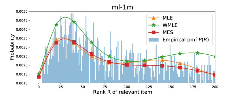
Figure 1: Learning Empirical Rank Distribution $P(R)$

Sampling Rank Distribution: Mixtures of Binomial Distributions

To simplify our discussion, let us consider the sampling with replacement scheme (the results can be extended to sampling without replacement). Now, assume an item $i$ is ranked $R$ in the entire set of items $I$. Then there are $R-1$ items whose rank is higher than item $i$ and $N-R$ items whose rank is lower than $i$. Under the (uniform) sampling (sampling with replacement), we have $\theta\coloneqq\frac{R-1}{N-1}$ probability to pick up an item with higher rank than $R$. Let $x$ be the number of irrelevant items ranked in front of the relevant one, and $x=r-1$. Thus, the rank $r-1$ under sampling follows a binomial distribution: $r-1\sim B(n-1,\theta)$, and the conditional rank distribution $P(r|R)$ is

$$\begin{split}&P(r|R)=Bin(r-1;n-1,\theta)=\binom{n-1}{r-1}\theta^{r-1}(1-\theta)^{n-r}\end{split}$$ (16)

Given this, an interesting observation is that the sampling ranked data $\{r_{u}\}_{r=1}^{M}$ can be directly modeled as a mixture of binomial distributions. Let $\boldsymbol{\Theta}=(\theta_{1}\dots,\theta_{R},\dots,\theta_{N})^{T}$ where

$$\theta_{R}\coloneqq\frac{R-1}{N-1},\quad R=1,\dots,N$$ (17)

Let the empirical rank distribution $\boldsymbol{P}=(P(R))_{R=1}^{N}$, then the sampling rank follows the distribution $P(r|\boldsymbol{P})=$

$$\sum_{R=1}^{N}P(r|R)P(R)=\sum_{R=1}^{N}Bin(r-1;n-1,\theta_{R})P(R)$$

$$= \sum_{R=1}^{N}P(R)\binom{n-1}{r-1}\big{(}\frac{R-1}{N-1}\big{)}^{r-1}\big{(}1-\frac{R-1}{N-1}\big{)}^{n-r}$$ (18)

Thus, $P(R)$ can be considered as the parameters for the mixture of binomial distributions.

Maximum Likelihood Estimation

The basic approach to learn the parameters of the mixture of binomial distributions ($MB$) given $\{r_{u}\}_{u=1}^{M}$ is based on maximal likelihood estimation (MLE). Let $\boldsymbol{\Pi}=(\pi_{1},\dots,\pi_{R},\dots,\pi_{N})^{T}$ be the parameters of the mixture of binomial distributions. Then we have $p(r_{u}|\boldsymbol{\Pi})=\sum_{R=1}^{N}\pi_{R}p(r_{u}|\theta_{R})$, where $p(r_{u}|\theta_{R})=Bin(r_{u}-1;n-1,\theta_{R})$.

Then MLE aims to find the particular $\boldsymbol{\Pi}$, which maximizes the log-likelihood:

$$\log\mathcal{L}=\sum\limits_{u=1}^{M}{\log{p(r_{u}|\boldsymbol{\Pi})}}=\sum\limits_{u=1}^{M}{\log{\sum_{R=1}^{N}\pi_{R}p(r_{u}|\theta_{R})}}$$ (19)

By leveraging EM algorithm (see Appendix for details), we have:

$$\pi^{new}_{R}=\frac{1}{M}\sum\limits_{u=1}^{M}\frac{{\pi}^{old}_{R}p(r_{u}|\theta_{R})}{\sum\limits_{j=1}^{N}{\pi^{old}_{j}p(r_{u}|\theta_{j})}}$$ (20)

When eq. 20 converges, we obtain $\boldsymbol{\Pi}^{*}$ and use it to estimate $\boldsymbol{P}$, i.e., $\widehat{P}(R)=\pi^{*}_{R}$. Then, we can use $\widehat{P}(R)$ in eq. 14 to estimate the desired metric $metric@K$.

Speedup and Time Complexity

To speedup the computation, we can further rewrite the updated formula eq. 20 as

$$\pi^{new}_{R}=\sum\limits_{r=1}^{n}\tilde{P}(r)\frac{{\pi}^{old}_{R}p(r|\theta_{R})}{\sum\limits_{j=1}^{N}{\pi^{old}_{j}p(r|\theta_{j})}}$$ (21)

where $\tilde{P}(r)=\frac{1}{M}\sum_{u=1}^{M}{\bf 1}_{r_{u}=r}$ is the empirical rank distribution on the sampling data. Thus the time complexity improves to $O(kNn)$ (from $O(kNM)$ using eq. 20) where $k$ is the iteration number. This is faster than the least squares solver for the $BV$ estimator (eq. 11)  (Krichene and Rendle 2020), which is at least $O(n^{2}N)$.Furthermore, we note $\widehat{P}(R)$ can be used for any $metric@K$ for the same algorithm, whereas $BV$ estimator has to be performed for each $metric@K$ separately.

Weighted MLE

If we are particularly interested in $\pi_{R}$ ($P(R)$) when $R$ is very small (such as $R<10$), then we can utilize the weighted MLE to provide more focus on those ranks. This is done by putting more weight on the sampling rank observation $r_{u}$ when $r_{u}$ is small. Specifically, the weighted MLE aims to find the $\boldsymbol{\Pi}$, which maximizes the weighted log-likelihood:

$$\log\mathcal{L}=\sum\limits_{u=1}^{M}{w(r_{u})\log{p(r_{u}|\boldsymbol{\Pi})}}=\sum\limits_{u=1}^{M}{w(r_{u})\log{\sum_{R=1}^{N}\pi_{R}p(r_{u}|\theta_{R})}}$$ (22)

where $w(r_{u})$ is the weight for user $u$. Note that the typical MLE (without weight) is the special case of eq. 22 ($w(r_{u})=1$).

For weighted MLE, its updated formula is

$$\pi^{new}_{R}=\sum\limits_{r=1}^{n}\frac{\tilde{P}(r)w(r)}{\sum_{r=1}^{n}\tilde{P}(r)w(r)}\frac{{\pi}^{old}_{R}p(r|\theta_{R})}{\sum\limits_{j=1}^{N}{\pi^{old}_{j}p(r|\theta_{j})}}$$ (23)

For the weight $w_{u}$, we can utilize any decay function (as $r_{u}$ becomes bigger, than $w_{u}$ will reduce). We have experimented with various decay functions and found that the important/metric functions, such as $AP$ and $NDCG$, $w_{u}=\mathcal{M}_{AP}(r_{u}/C)$ and $w_{u}=\mathcal{M}_{NDCG}(r_{u}/C)$ ($C>1$ is a constant to help reduce the decade rate), obtain good and competitive results. We will provide their results in the experimental evaluation section.

Maximal Entropy with Minimal Distribution Bias

Another commonly used approach for estimating a (discrete) probability distribution is based on the principal of maximal entropy (Cover and Thomas 2006). Assume a random variable $x$ takes values in $(x_{1},x_{2},\cdots,x_{n})$ with pmf: $p(x_{1}),p(x_{2}),\cdots,p(x_{n})$. Typically, given a list of (linear) constraints in the form of $\sum_{i=1}^{n}p(x_{i})f_{k}(x_{i})\geq F_{k}$ ($k=1,\cdots m$), together with the equality constraint ($\sum_{i=1}^{n}p(x_{i})=1$), it aims to maximize its entropy:

$$H(p)=-\sum_{i=1}^{n}p(x_{i})\log p(x_{i})$$ (24)

In our problem, let the random variable $\mathcal{R}$ take on rank from $1$ to $N$. Assume its pmf is $\boldsymbol{\Pi}=(\pi_{1},\dots,\pi_{R},\dots,\pi_{N})$, and the only immediate inequality constraint is $\pi_{R}\geq 0$ besides $\sum_{R=1}^{N}\pi_{R}=1$. Now, to further constrain $\boldsymbol{\pi}$, we need to consider how they reflect and manifest on the observation data $\{r_{u}\}^{M}_{u=1}$. The natural solution is to simply utilize the (log) likelihood. However, combining them together leads to a rather complex non-convex optimization problem which will complicate the EM-solver.

In this paper, we introduce a method (to constrain the maximal entropy) which utilizes the squared distance between the learned rank probability (based on $\boldsymbol{\Pi}$) and the empirical rank probability in the sampling data

$$\begin{split}\mathcal{E}&=\frac{1}{M}\sum\limits_{R=1}^{M}{\Big{(}p(r_{u}|\boldsymbol{\Pi})-\tilde{P}(r_{u})\Big{)}^{2}}\\ &=\sum\limits_{r=1}^{n}{\tilde{P}(r)\Big{(}\sum\limits_{R=1}^{N}{P(r|R)\pi_{R}}-\tilde{P}(r)\Big{)}^{2}}\end{split}$$ (25)

Again, $\tilde{P}(r)$ is the empirical rank distribution in the sampling data. Note that $\mathcal{E}$ can be considered to be derived from the log-likelihood of independent Gaussian distributions if we assume the error term $p(r_{u}|\boldsymbol{\Pi})-\tilde{P}(r_{u})$ follows the Gaussian distribution.

Given this, we seek to solve the following optimization problem:

$$\boldsymbol{\Pi}=\arg\max_{\boldsymbol{\Pi}}\eta\cdot H(\boldsymbol{\pi})-\mathcal{E}$$ (26)

with constraints:

$$\pi_{R}\geq 0\ (1\leq R\leq N)\ \ \ \ \sum_{R}{\pi_{R}}=1$$ (27)

Note that this objective can also be considered as adding an entropy regularizer for the log-likelihood.

The objective function: $\eta\cdot H(\boldsymbol{\pi})-\mathcal{E}$ is concave (or its negative is convex). This can be easily observed as both negative of entropy and sum of squared errors are convex function.

Given this, we can employ available convex optimization solvers (Boyd and Vandenberghe 2004) to identify the optimization solution. Thus, we have the estimator $\widehat{P}(R)=\pi^{*}_{R}$, where $\Pi^{*}$ is the optimal solution for eq. 26.

Model	Metric	Exact	Estimators of $Metrics@10$
			CLS	BV 0.1	BV 0.01	MLE	WMLE	MES
EASE	Recall	34.77	54.43$\scriptstyle\pm$1.29	36.83$\scriptstyle\pm$2.09	36.18$\scriptstyle\pm$5.35	35.33$\scriptstyle\pm$7.17	36.30$\scriptstyle\pm$7.41	35.22$\scriptstyle\pm$7.36
	NDCG	16.16	25.44$\scriptstyle\pm$0.60	16.81$\scriptstyle\pm$1.04	16.38$\scriptstyle\pm$2.88	16.03$\scriptstyle\pm$3.95	16.46$\scriptstyle\pm$4.07	16.03$\scriptstyle\pm$4.12
	AP	10.63	16.81$\scriptstyle\pm$0.40	10.88$\scriptstyle\pm$0.72	10.53$\scriptstyle\pm$2.13	10.32$\scriptstyle\pm$2.97	10.59$\scriptstyle\pm$3.06	10.35$\scriptstyle\pm$3.13
MultiVAE	Recall	18.38	45.23$\scriptstyle\pm$1.42	26.27$\scriptstyle\pm$2.46	21.66$\scriptstyle\pm$6.11	20.79$\scriptstyle\pm$6.78	21.23$\scriptstyle\pm$6.96	20.58$\scriptstyle\pm$6.97
	NDCG	7.08	21.13$\scriptstyle\pm$0.66	11.80$\scriptstyle\pm$1.22	9.38$\scriptstyle\pm$3.26	9.17$\scriptstyle\pm$3.44	9.35$\scriptstyle\pm$3.53	9.10$\scriptstyle\pm$3.58
	AP	3.81	13.97$\scriptstyle\pm$0.44	7.53$\scriptstyle\pm$0.85	5.77$\scriptstyle\pm$2.39	5.74$\scriptstyle\pm$2.44	5.86$\scriptstyle\pm$2.50	5.72$\scriptstyle\pm$2.56
NeuMF	Recall	30.96	49.51$\scriptstyle\pm$1.31	32.12$\scriptstyle\pm$2.17	31.30$\scriptstyle\pm$5.63	31.06$\scriptstyle\pm$7.15	31.82$\scriptstyle\pm$7.37	30.63$\scriptstyle\pm$7.30
	NDCG	13.43	23.14$\scriptstyle\pm$0.61	14.62$\scriptstyle\pm$1.08	14.15$\scriptstyle\pm$3.03	14.16$\scriptstyle\pm$3.94	14.49$\scriptstyle\pm$4.05	13.99$\scriptstyle\pm$4.06
	AP	8.26	15.29$\scriptstyle\pm$0.40	9.44$\scriptstyle\pm$0.75	9.08$\scriptstyle\pm$2.24	9.15$\scriptstyle\pm$2.96	9.37$\scriptstyle\pm$3.04	9.06$\scriptstyle\pm$3.07
itemKNN	Recall	42.72	46.46$\scriptstyle\pm$1.28	34.26$\scriptstyle\pm$2.00	38.29$\scriptstyle\pm$5.09	40.02$\scriptstyle\pm$7.22	41.71$\scriptstyle\pm$7.56	39.20$\scriptstyle\pm$6.43
	NDCG	20.54	21.71$\scriptstyle\pm$0.60	15.80$\scriptstyle\pm$0.99	17.81$\scriptstyle\pm$2.74	18.96$\scriptstyle\pm$4.24	19.75$\scriptstyle\pm$4.43	18.53$\scriptstyle\pm$3.73
	AP	13.89	14.35$\scriptstyle\pm$0.40	10.32$\scriptstyle\pm$0.69	11.73$\scriptstyle\pm$2.02	12.68$\scriptstyle\pm$3.32	13.21$\scriptstyle\pm$3.47	12.38$\scriptstyle\pm$2.90
ALS	Recall	24.17	48.07$\scriptstyle\pm$1.20	29.62$\scriptstyle\pm$2.04	26.17$\scriptstyle\pm$5.64	25.16$\scriptstyle\pm$6.49	25.91$\scriptstyle\pm$6.72	24.94$\scriptstyle\pm$7.08
	NDCG	9.49	22.46$\scriptstyle\pm$0.56	13.39$\scriptstyle\pm$1.02	11.54$\scriptstyle\pm$3.08	11.18$\scriptstyle\pm$3.40	11.51$\scriptstyle\pm$3.52	11.14$\scriptstyle\pm$3.76
	AP	5.21	14.84$\scriptstyle\pm$0.37	8.59$\scriptstyle\pm$0.72	7.23$\scriptstyle\pm$2.30	7.06$\scriptstyle\pm$2.47	7.27$\scriptstyle\pm$2.55	7.08$\scriptstyle\pm$2.76

Table 2: Dataset: ml-1m with sample size =$99$.

Model	Metric	Exact	Estimators of $Metric@10$
			CLS	BV 0.1	BV 0.01	MLE	WMLE	MES
EASE	Recall	87.91	52.56$\scriptstyle\pm$0.52	49.62$\scriptstyle\pm$1.06	65.99$\scriptstyle\pm$2.98	83.19$\scriptstyle\pm$10.14	84.13$\scriptstyle\pm$10.26	83.72$\scriptstyle\pm$11.83
	NDCG	43.63	24.04$\scriptstyle\pm$0.24	22.70$\scriptstyle\pm$0.49	30.28$\scriptstyle\pm$1.39	38.55$\scriptstyle\pm$4.97	38.99$\scriptstyle\pm$5.03	38.83$\scriptstyle\pm$5.81
	AP	30.48	15.58$\scriptstyle\pm$0.15	14.73$\scriptstyle\pm$0.32	19.70$\scriptstyle\pm$0.92	25.29$\scriptstyle\pm$3.42	25.58$\scriptstyle\pm$3.46	25.49$\scriptstyle\pm$4.01
MultiVAE	Recall	48.82	55.62$\scriptstyle\pm$0.54	52.84$\scriptstyle\pm$1.10	70.09$\scriptstyle\pm$2.96	86.45$\scriptstyle\pm$9.89	86.98$\scriptstyle\pm$9.95	87.02$\scriptstyle\pm$10.82
	NDCG	17.12	25.43$\scriptstyle\pm$0.25	24.17$\scriptstyle\pm$0.51	32.16$\scriptstyle\pm$1.38	39.98$\scriptstyle\pm$4.82	40.22$\scriptstyle\pm$4.85	40.27$\scriptstyle\pm$5.29
	AP	8.14	16.49$\scriptstyle\pm$0.16	15.68$\scriptstyle\pm$0.33	20.92$\scriptstyle\pm$0.91	26.18$\scriptstyle\pm$3.30	26.34$\scriptstyle\pm$3.32	26.39$\scriptstyle\pm$3.63
NeuMF	Recall	62.87	45.83$\scriptstyle\pm$0.56	41.51$\scriptstyle\pm$1.12	53.39$\scriptstyle\pm$3.16	63.68$\scriptstyle\pm$9.42	64.24$\scriptstyle\pm$9.52	64.39$\scriptstyle\pm$11.44
	NDCG	31.05	20.96$\scriptstyle\pm$0.26	18.98$\scriptstyle\pm$0.52	24.48$\scriptstyle\pm$1.48	29.41$\scriptstyle\pm$4.58	29.67$\scriptstyle\pm$4.62	29.77$\scriptstyle\pm$5.59
	AP	21.66	13.59$\scriptstyle\pm$0.17	12.30$\scriptstyle\pm$0.34	15.91$\scriptstyle\pm$0.98	19.23$\scriptstyle\pm$3.13	19.41$\scriptstyle\pm$3.16	19.50$\scriptstyle\pm$3.83
itemKNN	Recall	68.46	52.88$\scriptstyle\pm$0.52	50.42$\scriptstyle\pm$1.03	68.04$\scriptstyle\pm$3.08	88.43$\scriptstyle\pm$11.35	89.36$\scriptstyle\pm$11.48	89.19$\scriptstyle\pm$13.13
	NDCG	28.71	24.18$\scriptstyle\pm$0.24	23.07$\scriptstyle\pm$0.48	31.23$\scriptstyle\pm$1.44	41.06$\scriptstyle\pm$5.59	41.49$\scriptstyle\pm$5.66	41.46$\scriptstyle\pm$6.49
	AP	17.12	15.68$\scriptstyle\pm$0.15	14.97$\scriptstyle\pm$0.31	20.32$\scriptstyle\pm$0.95	26.98$\scriptstyle\pm$3.86	27.27$\scriptstyle\pm$3.91	27.28$\scriptstyle\pm$4.49
ALS	Recall	58.55	31.39$\scriptstyle\pm$0.48	26.90$\scriptstyle\pm$0.93	34.43$\scriptstyle\pm$2.62	42.21$\scriptstyle\pm$7.16	43.05$\scriptstyle\pm$7.31	43.09$\scriptstyle\pm$8.91
	NDCG	30.30	14.35$\scriptstyle\pm$0.22	12.29$\scriptstyle\pm$0.43	15.78$\scriptstyle\pm$1.22	19.55$\scriptstyle\pm$3.50	19.94$\scriptstyle\pm$3.57	20.00$\scriptstyle\pm$4.39
	AP	21.77	9.31$\scriptstyle\pm$0.14	7.97$\scriptstyle\pm$0.28	10.26$\scriptstyle\pm$0.81	12.82$\scriptstyle\pm$2.40	13.07$\scriptstyle\pm$2.45	13.14$\scriptstyle\pm$3.02

Table 3: Dataset: citeulike with sample size =$99$.

Experiments

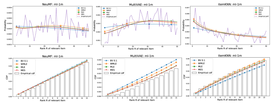
Figure 2: Accuracy of Learned Empirical Rank Distribution

In this section, we report the experimental evaluation on estimating the top-$K$ metrics based on sampling, as well as the learning of empirical rank distribution $P(R)$. Specifically, we aim to answer the following questions:

(Question 1) How do the new estimators based on the learned empirical distribution perform against the $CLS$ and $BV$ approach proposed in  (Krichene and Rendle 2020) on estimating the top-$K$ metrics based on sampling?

(Question 2) How do these approaches perform when helping predict the winners (from the global metrics) among a list of competitive recommendation algorithms using sampling?

(Question 3) How accurately can the proposed approaches learn the empirical rank distribution?

Experimental Setup

We use four of the most commonly used datasets for recommendation studies in our study, whose characteristics are in the Appendix. For the different recommendation algorithms, we use some of the most well-known and the state-of-the-art algorithms, including three non-deep-learning options: itemKNN (Deshpande and Karypis 2004); ALS (Hu, Koren, and Volinsky 2008); and EASE (Steck 2019); and two deep learning options: NeuMF (He et al. 2017) and MultiVAE (Liang et al. 2018). We use three (likely the most) commonly used top-K evaluation metrics: $Recall$, $NDCG$ and $AP$ (Average Precision). Due to the space limitation, we only report representative results here, and additional experimental results can be found in the Appendix.

Estimation Accuracy of Metric@$K$

Table 2 and 3 show the average and the standard deviation of the aforementioned estimators for $Recall@10$, $NDCG@10$, and $AP@10$, which repeats $100$ each with sample size $99$ ($n=100$). The estimators include $CLS$, $BV$ (with the tradeoff parameters $\gamma=0.1$ and $\gamma=0.01$), $MLE$ (Maximal Likelihood Estimation), $WMLE$ (Weighted Maximal Likelihood Estimation where the weighted function is $M_{NDCG}$ with $C=10$), $MES$ (Maximal Entropy with Squared distribution distance, where $\eta=0.001$). The $Exact$ column corresponds to the target metrics which use all items in $I$ for ranking.

In Table 2 on the $ml-1m$ dataset, we observe that $MLE$ and $MES$ are among the most, or the second-most accurate estimators (using the bias which measures the difference between the Exact Metrics and the Average of the Estimated Metrics). In Table 3, $WMLE$ performs the best, with $7$ most (or second-most) accurate estimations, whereas $MES$, $MB$, and $BV$ estimators are all comparable, with each having some better estimates. In both tables, $CLS$ estimator has the worst performance. In addition, we also notice that the new estimators tend to have higher variance than the $BV$ estimators, which explicitly control the variance of each individual ${\mathcal{M}}(r)$ estimate. In the future, we plan to utilize methods such as bootstrapping to help reduce the variance of these estimators based on the empirical rank distribution.

Predicting Winners by Metric@$K$

Table 4 shows, among the $100$ sample runs, the number of correct winners predicted by $CLS$, $BV$, $MLE$, $WLE$ and $MES$ estimators based on $Recall@K$, $NDCG@K$ and $AP@K$ for $K=1$, $5$, $10$ and $20$, on the $ml-1m$ dataset. We observe that $WMLE$ has the best prediction accuracy in picking up the winners, while $MLE$ and $MES$ are comparable and slightly better than $BV0.01$.

Learning Empirical Rank Distributions

Figure 2 illustrates the accuracy of learned empirical Rank Distributions against the exact $P(R)$ on the $ml-1m$ dataset for three recommendation methods: $NeuMF$, $MultiVAE$, and $itemKNN$, respectively. The empirical pmf refers to $P(R)$, and the estimation methods include $BV$ (with parameter $0.1$), $MLE$, $WMLE$, and $MES$. The three figures on the top show the (learned) probability mass function, whereas the bottom shows the corresponding CDF (or Recall) at the top-$K$. These estimation curves are the average of estimates of $100$ sample runs. We can see that $BV$ either over- or under- estimates the empirical CDF ($Recall$ curve). $MLE$ and $MES$ are quite comparable where $WMLE$ has a higher average estimate than both of them. This is understandable as we add more weight to the sampled rank with smaller values, which leads to a higher concentration of probability mass for the smaller rank. We also notice that all these estimators are not very accurate on the individual rank probability $P(R)$ (the top figures). But their aggregated results (CDF; the bottom figures) are quite accurate. This helps explain why we can estimate $metric@K$, which is also an aggregate. In the Appendix, we show that as the sample size increases, the estimate accuracy will also increase accordingly.

K	Metric	CLS	0.1	0.01	MLE	WMLE	MES
1	Recall	0	41	59	59	59	57
	NDCG	0	41	59	59	59	57
	AP	0	41	59	59	59	57
5	Recall	0	34	57	59	61	59
	NDCG	0	34	57	59	61	59
	AP	0	35	58	59	61	59
10	Recall	0	21	54	58	59	58
	NDCG	0	24	56	60	61	59
	AP	0	27	56	61	61	59
20	Recall	100	98	59	49	45	53
	NDCG	0	4	51	54	58	53
	AP	0	23	53	60	61	58

Table 4: The number of successes at predicting a winner on the ml-1m dataset with 100 repeats. 0.1 and 0.01 represent the estimator BV with $\gamma=0.1$ and $0.01$ correspondingly.

Conclusion

In this paper, we study a new approach to estimate the top-$K$ evaluation metrics based on learning the empirical rank distribution from sampling, which is, by itself, a new and interesting research problem. We present two approaches based on Maximal Likelihood Estimation and Maximal Entropy principals. Our experimental results show the advantage of using the new approaches to estimate the top-$K$ metrics. In our future work, we plan to investigate the open questions on how many samples we should use for recovering the empirical rank distribution and top-$K$ metrics.

Appendix A Dataset Statistics

In table  5, we describe the information of the dataset we used.

Dataset	Interactions	Users	Items	Sparsity
ml-1m	1,000,209	6,040	3,706	95.53$\%$
pinterest-20	1,463,581	55,187	9,916	99.73$\%$
citeulike	204,986	5,551	16,980	99.78$\%$
yelp	696,865	25,677	25,815	99.89$\%$

Table 5: Dataset Statistics

Appendix B EM Algorithm for Mixtures of Binomial Model

In this section, we give the details of the EM algorithm for $MLE$ estimator. Recall eq. 22 Weighted log-likelihood function is:

$$\log{\mathcal{L}}=\sum\limits_{u=1}^{M}{w_{u}\log{\sum\limits_{k=1}^{N}{p(x_{u},z_{uk}|\theta_{k})}}}$$

E-step

$$\mathcal{Q}(\boldsymbol{\pi},\boldsymbol{\pi}^{old})=\sum\limits_{u=1}^{M}{w_{u}\sum\limits_{k=1}^{N}{\gamma(z_{uk})\log{p(x_{u},z_{uk}|\theta_{k})}}}$$

where

$$\gamma(z_{uk})=p(z_{uk}|x_{u},\boldsymbol{\pi}^{old})=\frac{{\pi}^{old}_{k}p(x_{u}|\theta_{k})}{\sum\limits_{j=1}^{N}{\pi^{old}_{j}p(x_{u}|\theta_{j})}}$$

M-step

$$\mathcal{Q}^{\prime}(\boldsymbol{\pi},\boldsymbol{\pi}^{old})=\mathcal{Q}(\boldsymbol{\pi},\boldsymbol{\pi}^{old})+\lambda(1-\sum\limits_{k=1}^{N}{\pi_{k}})$$ (28)

$$\frac{\partial\mathcal{Q}^{\prime}(\boldsymbol{\pi},\boldsymbol{\pi}^{old})}{\partial\pi_{k}}=\sum\limits_{u=1}^{M}{\frac{w_{u}\gamma(z_{uk})}{\pi_{k}}-\lambda}=0$$

$$\lambda\pi_{k}=\sum\limits_{u=1}^{M}{w_{u}\cdot\gamma(z_{uk})}$$

$$\lambda=\sum\limits_{k=1}^{N}\sum\limits_{u=1}^{M}{w_{u}\cdot\gamma(z_{uk})}=\sum\limits_{u=1}^{M}{w_{u}}$$ (29)

$$\pi^{new}_{k}=\frac{\sum\limits_{u=1}^{M}{w_{u}\cdot\gamma(z_{uk})}}{\sum\limits_{u=1}^{M}{w_{u}}}$$

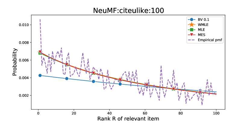
(a)

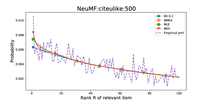
(b)

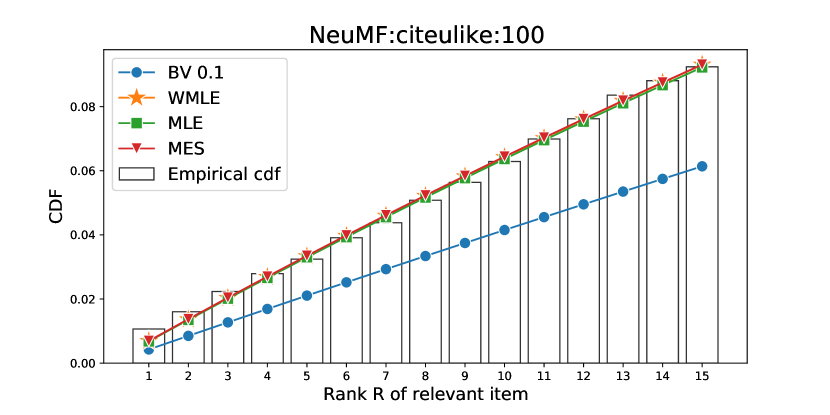
(c)

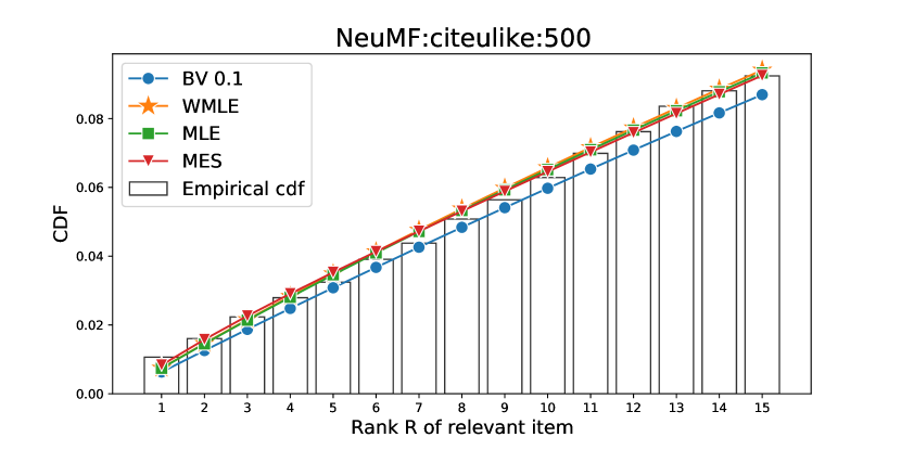
(d)

Figure 3: Accuracy of Learned Empirical Rank Distribution with Different Sample Size. The experiments are carryied on dataset $citeulike$ with recommender $NeuMF$. $100$ and $500$ indicate the sample size is $99$ and $499$ respectively. As the sample size increases, the estimation curves tend to get closer to the empirical rank curve, especially for the $BV0.1$ estimator.

Appendix C Sample Size Impact Accuracy

Figure 3 illustrates the accuracy of learned empirical Rank Distributions against the exact $P(R)$ on the $citeulike$ dataset for recommender $NeuMF$. Figure  3(a) and  3(b) show the probability mass function with sample size 99 (n = 100) and 499 (n = 500) respectively. Similarly, Figure  3(c) and  3(d) display the corresponding CDF at the top-$K$. These estimation curves are the average of estimates of $100$ sample runs. From the figures, we can see that, as the sample size increases, the estimation curves get close to the empirical distribution. That’s to say, as the sample size increases, the estimate accuracy will also increase accordingly.

Appendix D Estimation Accuracy of Metric@$K$

Table 6 and  7 show the average and the standard deviation of the aforementioned estimators for $Recall@10$, $NDCG@10$, and $AP@10$, which runs $100$ samples each with sample size $99$ ($n=100$).

In Table 6 on the $pinterest-20$ dataset and table 7 on the $yelp$ dataset, we observe that $MLE$ and $MES$ are pretty much accurate than $BV$ estimator.

Overall, $MLE$ and $MES$ can produce more accurate estimation of metrics than $BV$ with higher variance.

Model	Metric	Exact	Estimators of $Metric@10$
			BV 0.1	BV 0.01	MLE	WMLE	MES
EASE	Recall	52.11	38.61$\scriptstyle\pm$0.42	44.85$\scriptstyle\pm$1.33	48.31$\scriptstyle\pm$2.77	48.61$\scriptstyle\pm$2.79	48.79$\scriptstyle\pm$3.85
	NDCG	26.19	17.67$\scriptstyle\pm$0.20	20.59$\scriptstyle\pm$0.64	22.29$\scriptstyle\pm$1.38	22.43$\scriptstyle\pm$1.39	22.55$\scriptstyle\pm$1.95
	AP	18.46	11.46$\scriptstyle\pm$0.13	13.40$\scriptstyle\pm$0.43	14.57$\scriptstyle\pm$0.96	14.66$\scriptstyle\pm$0.97	14.76$\scriptstyle\pm$1.38
MultiVAE	Recall	24.63	36.13$\scriptstyle\pm$0.48	37.46$\scriptstyle\pm$1.30	36.01$\scriptstyle\pm$2.16	36.14$\scriptstyle\pm$2.17	34.28$\scriptstyle\pm$3.01
	NDCG	9.72	16.49$\scriptstyle\pm$0.23	17.07$\scriptstyle\pm$0.62	16.34$\scriptstyle\pm$1.04	16.40$\scriptstyle\pm$1.05	15.49$\scriptstyle\pm$1.47
	AP	5.39	10.68$\scriptstyle\pm$0.15	11.04$\scriptstyle\pm$0.42	10.52$\scriptstyle\pm$0.71	10.55$\scriptstyle\pm$0.71	9.93$\scriptstyle\pm$1.00
NeuMF	Recall	41.91	34.82$\scriptstyle\pm$0.51	38.94$\scriptstyle\pm$1.36	40.55$\scriptstyle\pm$2.45	40.74$\scriptstyle\pm$2.46	40.40$\scriptstyle\pm$3.58
	NDCG	19.75	15.92$\scriptstyle\pm$0.24	17.83$\scriptstyle\pm$0.65	18.61$\scriptstyle\pm$1.21	18.70$\scriptstyle\pm$1.21	18.55$\scriptstyle\pm$1.80
	AP	13.14	10.32$\scriptstyle\pm$0.16	11.58$\scriptstyle\pm$0.44	12.11$\scriptstyle\pm$0.83	12.16$\scriptstyle\pm$0.84	12.07$\scriptstyle\pm$1.26
itemKNN	Recall	52.53	39.04$\scriptstyle\pm$0.42	45.30$\scriptstyle\pm$1.21	48.68$\scriptstyle\pm$2.47	48.91$\scriptstyle\pm$2.49	48.96$\scriptstyle\pm$3.54
	NDCG	26.23	17.87$\scriptstyle\pm$0.20	20.79$\scriptstyle\pm$0.58	22.45$\scriptstyle\pm$1.23	22.56$\scriptstyle\pm$1.24	22.61$\scriptstyle\pm$1.79
	AP	18.38	11.59$\scriptstyle\pm$0.13	13.53$\scriptstyle\pm$0.39	14.67$\scriptstyle\pm$0.86	14.74$\scriptstyle\pm$0.86	14.79$\scriptstyle\pm$1.26
ALS	Recall	43.40	34.34$\scriptstyle\pm$0.43	39.26$\scriptstyle\pm$1.17	41.77$\scriptstyle\pm$2.24	42.32$\scriptstyle\pm$2.27	41.90$\scriptstyle\pm$3.21
	NDCG	20.62	15.71$\scriptstyle\pm$0.20	18.01$\scriptstyle\pm$0.56	19.23$\scriptstyle\pm$1.11	19.48$\scriptstyle\pm$1.13	19.31$\scriptstyle\pm$1.62
	AP	13.83	10.19$\scriptstyle\pm$0.13	11.71$\scriptstyle\pm$0.38	12.54$\scriptstyle\pm$0.77	12.71$\scriptstyle\pm$0.78	12.61$\scriptstyle\pm$1.14

Table 6: Dataset: pinterest-20 with sample size =$99$.

Model	Metric	Exact	Estimators of $Metric@10$
			BV 0.1	BV 0.01	MLE	WMLE	MES
EASE	Recall	25.548	17.00$\scriptstyle\pm$0.26	21.30$\scriptstyle\pm$0.81	25.31$\scriptstyle\pm$2.24	25.78$\scriptstyle\pm$2.28	25.59$\scriptstyle\pm$2.87
	NDCG	11.848	7.75$\scriptstyle\pm$0.12	9.73$\scriptstyle\pm$0.38	11.62$\scriptstyle\pm$1.06	11.83$\scriptstyle\pm$1.08	11.75$\scriptstyle\pm$1.36
	AP	7.794	5.01$\scriptstyle\pm$0.08	6.30$\scriptstyle\pm$0.25	7.56$\scriptstyle\pm$0.71	7.69$\scriptstyle\pm$0.72	7.65$\scriptstyle\pm$0.91
MultiVAE	Recall	15.383	15.57$\scriptstyle\pm$0.25	18.79$\scriptstyle\pm$0.73	21.05$\scriptstyle\pm$1.81	21.38$\scriptstyle\pm$1.84	21.21$\scriptstyle\pm$2.26
	NDCG	5.741	7.10$\scriptstyle\pm$0.11	8.57$\scriptstyle\pm$0.34	9.63$\scriptstyle\pm$0.85	9.78$\scriptstyle\pm$0.87	9.71$\scriptstyle\pm$1.07
	AP	2.943	4.59$\scriptstyle\pm$0.07	5.55$\scriptstyle\pm$0.22	6.25$\scriptstyle\pm$0.57	6.35$\scriptstyle\pm$0.58	6.30$\scriptstyle\pm$0.71
NeuMF	Recall	21.381	13.84$\scriptstyle\pm$0.24	16.61$\scriptstyle\pm$0.69	18.56$\scriptstyle\pm$1.62	18.86$\scriptstyle\pm$1.64	18.61$\scriptstyle\pm$2.00
	NDCG	10.094	6.31$\scriptstyle\pm$0.11	7.58$\scriptstyle\pm$0.32	8.49$\scriptstyle\pm$0.76	8.63$\scriptstyle\pm$0.77	8.52$\scriptstyle\pm$0.94
	AP	6.739	4.08$\scriptstyle\pm$0.07	4.91$\scriptstyle\pm$0.21	5.51$\scriptstyle\pm$0.51	5.60$\scriptstyle\pm$0.51	5.53$\scriptstyle\pm$0.63
itemKNN	Recall	35.129	19.90$\scriptstyle\pm$0.31	25.68$\scriptstyle\pm$0.98	31.85$\scriptstyle\pm$3.02	32.40$\scriptstyle\pm$3.08	32.51$\scriptstyle\pm$3.79
	NDCG	16.258	9.08$\scriptstyle\pm$0.14	11.74$\scriptstyle\pm$0.45	14.65$\scriptstyle\pm$1.43	14.90$\scriptstyle\pm$1.46	14.97$\scriptstyle\pm$1.81
	AP	10.670	5.87$\scriptstyle\pm$0.09	7.61$\scriptstyle\pm$0.30	9.55$\scriptstyle\pm$0.96	9.71$\scriptstyle\pm$0.98	9.76$\scriptstyle\pm$1.22
ALS	Recall	20.057	15.04$\scriptstyle\pm$0.28	18.60$\scriptstyle\pm$0.80	21.77$\scriptstyle\pm$2.08	22.56$\scriptstyle\pm$2.16	22.02$\scriptstyle\pm$2.41
	NDCG	8.545	6.86$\scriptstyle\pm$0.13	8.49$\scriptstyle\pm$0.37	9.98$\scriptstyle\pm$0.98	10.35$\scriptstyle\pm$1.02	10.11$\scriptstyle\pm$1.14
	AP	5.131	4.43$\scriptstyle\pm$0.08	5.50$\scriptstyle\pm$0.24	6.49$\scriptstyle\pm$0.65	6.73$\scriptstyle\pm$0.68	6.57$\scriptstyle\pm$0.76

Table 7: Dataset: yelp with sample size =$99$.

Appendix E Predicting Winners by Metric@$K$

Table 8, 9 and  10 show, among the $100$ sample runs, the number of correct winners (algorithm with best performance) predicted by $BV$, $MLE$, $WLE$ and $MES$ estimators based on $Recall@K$, $NDCG@K$ and $AP@K$ for $K=1$, $5$, $10$ and $20$, on the $pinterest-20$, $yelp$ and $citeulike$ dataset respectively.

K	Metric	BV0.1	BV0.01	MLE	WMLE	MES
1	Recall	0	5	22	22	28
	NDCG	0	5	22	22	28
	AP	0	5	22	22	28
5	Recall	0	5	21	21	27
	NDCG	0	5	21	22	28
	AP	0	5	21	22	28
10	Recall	0	5	18	19	26
	NDCG	0	5	19	19	26
	AP	0	5	20	21	27
20	Recall	0	3	12	13	19
	NDCG	0	4	15	16	25
	AP	0	5	18	19	26

Table 8: The number of successes at predicting a winner on the citeulike dataset with 100 repeats.

K	Metric	BV0.1	BV0.01	MLE	WMLE	MES
1	Recall	100	100	97	97	94
	NDCG	100	100	97	97	94
	AP	100	100	97	97	94
5	Recall	100	100	97	97	94
	NDCG	100	100	97	97	94
	AP	100	100	97	97	94
10	Recall	100	100	97	97	94
	NDCG	100	100	97	97	94
	AP	100	100	97	97	94
20	Recall	100	100	99	99	97
	NDCG	100	100	99	99	96
	AP	100	100	97	97	94

Table 9: The number of successes at predicting a winner on the yelp dataset with 100 repeats.

K	Metric	BV0.1	BV0.01	MLE	WMLE	MES
1	Recall	17	36	46	46	48
	NDCG	17	36	46	46	48
	AP	17	36	46	46	48
5	Recall	86	64	55	55	48
	NDCG	16	36	45	45	49
	AP	16	36	45	45	49
10	Recall	86	66	57	55	51
	NDCG	86	65	57	53	50
	AP	14	36	45	45	48
20	Recall	87	69	61	59	56
	NDCG	87	66	59	56	52
	AP	86	66	56	55	50

Table 10: The number of successes at predicting a winner on the pinterest-20 dataset with 100 repeats.

References

- Boyd and Vandenberghe (2004) Boyd, S.; and Vandenberghe, L. 2004. Convex Optimization. Cambridge University Press. doi:10.1017/CBO9780511804441.
- Cover and Thomas (2006) Cover, T. M.; and Thomas, J. A. 2006. Elements of Information Theory (Wiley Series in Telecommunications and Signal Processing). USA: Wiley-Interscience. ISBN 0471241954.
- Cremonesi, Koren, and Turrin (2010) Cremonesi, P.; Koren, Y.; and Turrin, R. 2010. Performance of Recommender Algorithms on Top-n Recommendation Tasks. In RecSys’10.
- Dacrema, Cremonesi, and Jannach (2019) Dacrema, M. F.; Cremonesi, P.; and Jannach, D. 2019. Are We Really Making Much Progress? A Worrying Analysis of Recent Neural Recommendation Approaches. In Proceedings of the 13th ACM Conference on Recommender Systems, RecSys ’19.
- Deshpande and Karypis (2004) Deshpande, M.; and Karypis, G. 2004. Item-Based Top-N Recommendation Algorithms. ACM Trans. Inf. Syst. .
- Ebesu, Shen, and Fang (2018) Ebesu, T.; Shen, B.; and Fang, Y. 2018. Collaborative Memory Network for Recommendation Systems. In SIGIR’18.
- Gupta et al. (2020) Gupta, U.; Hsia, S.; Saraph, V.; Wang, X.; Reagen, B.; Wei, G.; Lee, H. S.; Brooks, D.; and Wu, C. 2020. DeepRecSys: A System for Optimizing End-To-End At-Scale Neural Recommendation Inference. In 2020 ACM/IEEE 47th Annual International Symposium on Computer Architecture (ISCA), 982–995.
- Harper and Konstan (2015) Harper, F. M.; and Konstan, J. A. 2015. The MovieLens Datasets: History and Context .
- He et al. (2017) He, X.; Liao, L.; Zhang, H.; Nie, L.; Hu, X.; and Chua, T.-S. 2017. Neural Collaborative Filtering. WWW ’17.
- Hu et al. (2018) Hu, B.; Shi, C.; Zhao, W. X.; and Yu, P. S. 2018. Leveraging Meta-Path Based Context for Top- N Recommendation with A Neural Co-Attention Model. In KDD’18.
- Hu, Koren, and Volinsky (2008) Hu, Y.; Koren, Y.; and Volinsky, C. 2008. Collaborative filtering for implicit feedback datasets. In ICDM’08.
- Koren (2008) Koren, Y. 2008. Factorization Meets the Neighborhood: A Multifaceted Collaborative Filtering Model. In KDD’08.
- Krichene et al. (2019) Krichene, W.; Mayoraz, N.; Rendle, S.; Zhang, L.; Yi, X.; Hong, L.; Chi, E. H.; and Anderson, J. R. 2019. Efficient Training on Very Large Corpora via Gramian Estimation. In ICLR’2019.
- Krichene and Rendle (2020) Krichene, W.; and Rendle, S. 2020. On Sampled Metrics for Item Recommendation. In Proceedings of the 26th ACM SIGKDD International Conference on Knowledge Discovery & Data Mining, KDD ’20.
- Lehmann and Casella (2006) Lehmann, E. L.; and Casella, G. 2006. Theory of point estimation. Springer Science & Business Media.
- Li et al. (2020) Li, D.; Jin, R.; Gao, J.; and Liu, Z. 2020. On Sampling Top-K Recommendation Evaluation. In Proceedings of the 26th ACM SIGKDD International Conference on Knowledge Discovery & Data Mining, KDD ’20.
- Liang et al. (2018) Liang, D.; Krishnan, R. G.; Hoffman, M. D.; and Jebara, T. 2018. Variational Autoencoders for Collaborative Filtering. In WWW’18.
- Rendle (2019) Rendle, S. 2019. Evaluation Metrics for Item Recommendation under Sampling.
- Rendle, Zhang, and Koren (2019) Rendle, S.; Zhang, L.; and Koren, Y. 2019. On the Difficulty of Evaluating Baselines: A Study on Recommender Systems .
- Steck (2019) Steck, H. 2019. Embarrassingly Shallow Autoencoders for Sparse Data. WWW’19 .
- Wang et al. (2019) Wang, X.; Wang, D.; Xu, C.; He, X.; Cao, Y.; and Chua, T. 2019. Explainable Reasoning over Knowledge Graphs for Recommendation. In The Thirty-Third AAAI Conference on Artificial Intelligence, AAAI2019.
- Yang et al. (2018a) Yang, L.; Bagdasaryan, E.; Gruenstein, J.; Hsieh, C.-K.; and Estrin, D. 2018a. OpenRec: A Modular Framework for Extensible and Adaptable Recommendation Algorithms. In WSDM’18.
- Yang et al. (2018b) Yang, L.; Cui, Y.; Xuan, Y.; Wang, C.; Belongie, S. J.; and Estrin, D. 2018b. Unbiased Offline Recommender Evaluation for Missing-Not-at-Random Implicit Feedback. In RecSys’18.