Anomalous fractional quantization in the kagomelike Heisenberg ladder:
Emergence of the effective spin-1 chain
Abstract
We study a Kagome-like spin- Heisenberg ladder with competing ferromagnetic (FM) and antiferromagnetic (AFM) exchange interactions. Using the density-matrix renormalization group based calculations, we obtain the ground state phase diagram as a function of the ratio between the FM and AFM exchange interactions. Five different phases exist. Three of them are spin polarized phases; an FM phase and two kinds of ferrimagnetic (FR) phases (referred to as FR1 and FR2 phases). The spontaneous magnetization per site is , , and in the FM, FR1, and FR2 phases, respectively. This can be understood from the fact that an effective spin-1 Heisenberg chain formed by the upper and lower leg spins has a three-step fractional quantization of the magnetization per site as , , and . In particular, an anomalous “intermediate” state of the effective spin-1 chain with the reduced Hilbert space of a spin from to dimensional is highly unexpected in the context of conventional spin-1 physics. Thus, surprisingly, the effective spin-1 chain behaves like a spin-1/2 chain with SU(2) symmetry. The remaining two phases are spin-singlet phases with translational symmetry breaking in the presence of valence bond formations. One of them is octamer-siglet phase with a spontaneous octamerization long-range order of the system, and the other is period-4 phase characterized by the magnetic superstructure with a period of four structural unit cells. In these spin-singlet phases, we find the coexistence of valence bond structure and gapless chain. Although this may be emerged through the order-by-disorder mechanism, there can be few examples of such a coexistence.
I Introduction
The low-dimensional quantum magnets on geometrically frustrated lattices have been studied extensively in the last decades [1]. A variety of phases in such lattices originate from the macroscopically degenerate classical ground states. The quantum fluctuations may cause the spontaneous lift of degeneracy, which is called “order-by-disorder” mechanism [2]. The representatives of this mechanism include the spontaneous breaking of the lattice translational symmetry, resulting in the valence bond solid (VBS) state [3, 4, 5, 6] as well as in the magnetic long-range order [7, 8, 9], and that of the SU(2) spin symmetry, resulting in the ferrimagnetic (FR) long-range order [10, 11]. Also, the quantum frustrations may cause disordered quantum phases as well; the quantum spin liquid state is one of such examples, which has been intensively studied in the context of topological phases [12, 13, 14, 15, 16].
The frustration has another interesting aspect in one-dimensional (1D) quantum spin systems. In general, the inclusion of geometrical frustrations deserves an inclusion of non-bipartite interactions in the system, whereby some theorems based on the bipartite nature of the quantum spin systems may be broken due to its quantum fluctuations. For example, FR phases have often been discussed on the basis of the Lieb-Mattis (LM) theorem [17], which assumes the bipartite lattice. The LM–type FR state is considered as the coexistence of ferromagnetic (FM) and antiferromagnetic (AFM) orders, and the total magnetization must be integer quantized. However, in some 1D quantum spin systems, a partially-polarized FR phase, which is characterized by a graduate change in the spontaneous magnetization, has been found [18, 19, 20, 11]. They are kinds of non-LM–type FR phase. It is known that the coexistence of FM order and quasi-long-range order of Tomonaga-Luttinger liquid plays an essential role to realize such a partially-polarized FR state [20]. Thus, 1D quantum spin systems consisting frustrated FM and AFM interactions should provide a platform for the discovery of novel quantum phases of matter.
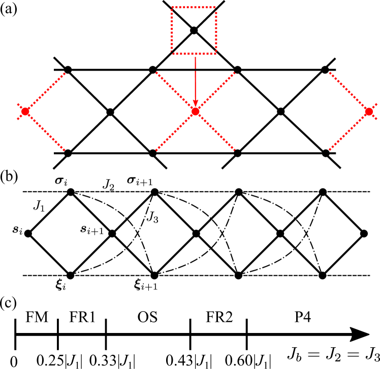
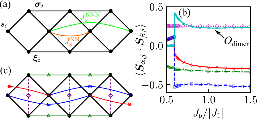
Recently, Dmitriev and Krivnov [21] studied a spin- FM-AFM Kagome-like ladder using numerical exact-diagonalization method on small clusters. The geometrical structure of this model is shown in Fig. 1(a), where the relevant FM-AFM exchange pattern is assumed to be in the parameter region of , and . When the AFM exchange interaction on the upper and lower legs () and that between the two legs () are both small in comparison with the nearest-neighbor FM exchange interaction (), this system is in a trivial FM phase. With increasing and , a phase transition from tge FM to FR states was found at based on the detailed analysis of the localized magnon states. In the FR state, the total magnetization of the system, i.e., total spin, is , where is the number of sites in the system.
The spin-1/2 Kagome-like ladder is a simplest spin model to describe a part of magnetic properties of the half-twisted ladder 334 compounds Ba3Cu3In4O12 and Ba3Cu3Sc4O12 [22, 23, 24, 25, 26]. These compounds exhibit similar fascinating phase diagrams with respect to the magnetic field and temperature. Of particular interest is that a series of spin-flop and spin-flip phase transitions as a function of the magnetic field has been observed at low temperature. To fully elucidate the nature of phase transitions, a deeper understanding of the ground state of the spin-1/2 Kagome-like ladder is necessary.
In this paper, we study the ground state of spin- FM-AFM Kagome-like ladder using the density-matrix renormalization group (DMRG) methods. We focus on the case of corresponding to the 334 compounds [22, 23, 24, 25, 26]. Based on the numerical calculations of total spin, static spin structure factor, spin-spin correlation functions, spin gap, dimer order parameter, and string order parameter, we find five different phases depending on . Three of them are spin polarized phases with spin rotation symmetry breaking; an FM phase and two kinds of FR phases (referred as FR1 and FR2 phases). The spontaneous magnetization per site is , , and in the FM, FR1, and FR2 phases, respectively. This can be understood from the fact that an effective spin-1 Heisenberg chain formed by the upper and lower leg spins has a fractional quantization of the magnetization per site as , , and . The origin of this anomalous quantization of the magnetization is explained in detail below. The remaining two phases are spin-singlet phases with translational symmetry breaking in the presence of valence bond formations. One of them is octamer-siglet (OS) phase with a spontaneous octamerization long-range order of the system, and the other is period-4 (P4) phase characterized by the magnetic superstructure with a period of four structural unit cells. We reveal the entire ground state phase diagram of the system as a function of , as is illustrated schematically in Fig. 1(c).
The paper is organized as follows: In Sec. II, we explain the spin-1/2 FM-AFM Kagome-like spin ladder and describe the numerical methods applied. In Sec. III, we study the total spin, spatial distribution of local magnetization, and spin-spin correlation functions to figure out fundamental features of the ground state. Then, we give the detailed discussion on each phase in Sec. IV. Summary is given in Sec. V.
II Model and Method
II.1 Model
The spin-1/2 Kagome-like Heisenberg ladder is defined as the three Heisenberg chains coupled with three types of Heisenberg exchange interactions , , and . The lattice structure and geometry of exchange interactions are illustrated in Fig. 1(a). The nearest-neighbor exchange interaction acts between the axial (or central) and leg spins, and the interaction acts between the neighboring spins in the upper and lower legs, while acts between the upper and lower leg spins in diagonal positions. The Hamiltonian is written as
| (1) | ||||
| (2) |
where , and are the spin- operators on the axial, upper-leg, and lower-leg sites in the unit cell , respectively. The system size is given by , where is the total number of the unit cells in the system. For convenience, we also use the notations , , , and . In some cases, it is beneficial to consider the system (2) divided into the axial-spin and leg-spin parts. We refer them as “axial-spin subsystem” and “leg-spin subsystem” hereafter.
We focus on the case where is FM (), and and are both AFM ( and ). In particular, we further restrict ourselves to the case at , which corresponds to the parameters for the half-twisted ladder 334 compounds Ba3Cu3In4O12 and Ba3Cu3Sc4O12 [22, 23, 24, 25, 26]. For simplicity, we define as . Only few theoretical studies have so far been performed on this case: Dmitriev and Krivnov [21] discussed the ground state manifold in the context of localized multimagnon states and the special multimagnon complexes. They also found a discontinuous phase transition from FM phase with to FR phase with at . Moreover, motivated by the experimental observations for the half-twisted ladder 334 compounds, Kumar et al. [25] studied the temperature and field dependent magnetism focusing on the paramagnetic phase. Yet, little is known about the -dependent ground-state phase diagram of the spin-1/2 Kagome-like ladder. Therefore, it is important to determine its ground state for better understanding of the magnetic properties of the half-twisted ladder 334 compounds.
A key factor to understand the ground state of spin-1/2 FM-AFM Kagome-like ladder is a formation of effective spin-1 degrees of freedom with the upper and lower leg spins, i.e., and . Note that the system [Eq.(2)] is invariant under interchange of the positions of and although it is a natural consequence of the formation of effective spin-1 degrees of freedom. Therefore, the two spins and are always equivalent and the correlation between the two sites is independently of , i.e., . As described in detail below, the combination of spin-1 degrees of freedom and order-by-disorder mechanism yields a variety of exotic magnetisms.
Furthermore, if we consider various combinations of FM or AFM parameters in the spin-1/2 Kagome-like Heisenberg ladder, an unexpected geometrical frustration may give rise to a huge variety of phases. For example, even in a simple case of , , , several exotic phases have been found: Waldtmann et al. [27] reported a LM–type FR phase with magnetization per site of at and a gapped period-6 VBS order at . Also, M-Aghaei et al. [28] identified some exotic gapless phases in the region of . The cases other than , , are beyond the scope of this paper but the systematic investigations appear to be intriguing future studies.
II.2 DMRG methods
We employ the matrix-product-state (MPS)-based DMRG and infinite-size DMRG (iDMRG) methods to examine the ground state of the spin-1/2 FM-AFM Kagome-like Heisenberg ladder shown in Fig. 1(a). We use the ITensor libraries [29] for numerical computations. Due to the severely frustrating nature of the present model, the finite-size scaling analysis may not be a straightforward task. We therefore use three boundary conditions in complementary style: The periodic boundary conditions (PBC) for the lattices with length up to (or ) are used to avoid unphysical edge effects. The open boundary conditions (OBC) for the lattices with length up to (or ) are used to obtain accurate numerical results. And, the iDMRG method (or the infinite-size boundary condition), which is efficient for calculating commensurate phases, is also used to directly obtain the physical quantities in the thermodynamic limit [30, 31]. Since there are a number of nearly degenerate states around the ground state due to the FM interaction and strong frustration, a relatively large number of density-matrix eigenstates needs to be kept in the renormalization procedure to obtain accurate results. In this paper, we keep up to density-matrix eigenstates, sweeping the MPSs until obtaining the ground states within the errors of and for the DMRG and iDMRG, respectively. Furthermore, the extrapolation is made with respect to when necessary.
III Results of calculations
In this section, we study the total spin, spatial distribution of local magnetization, and spin-spin correlation function as a preliminary step in elucidating the ground state of our system [Eq.(2)].
III.1 Total spin and magnetization
First, in order to see the parameter dependence of spontaneous magnetization, we calculate the total spin as a function of using the DMRG method for OBC and PBC clusters. The total spin can be estimated from the sum of spin-spin correlation functions over the system, namely,
| (3) |
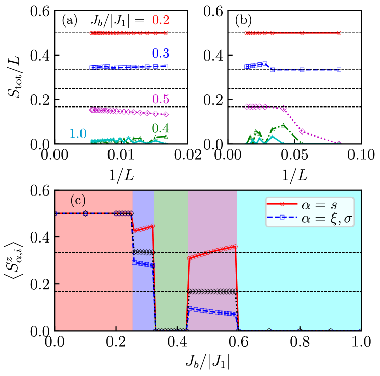
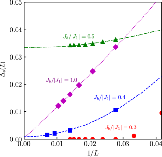
where () is the total spin operator. In Fig. 2 (a)[(b)], the finite-size scaling analysis of calculated with the OBC [PBC] is performed for several values of . Although the size dependence of is not very straightforward due to the strong frustration, we obtain the same extrapolated values of for the OBC and PBC in the thermodynamic limit : , , , , and for , , , , and , respectively. This coincidence of the extrapolated values between OBC and PBC gives a good indication to confirm the validity of the finite-size scaling analysis. As a result, we find that the ground state of our system is categorized into five regions by the values of as a function of : (i) (), (ii) (), (iii) (), (iv) (), (v) (). Since all of the obtained values indicate commensurate magnetic structures, we may explicitly define the magnetic unit cell in the whole region. It enables us to perform iDMRG simulation, which works directly in the thermodynamic limit, by assuming proper translational symmetry. Thus, we have confirmed the thermodynamic-limit values of between three independent calculations, i.e., OBC, PBC, and iDMRG.
Next, we calculate the expectation value of -component of spin operator to see the real-space distribution of the local magnetization using the iDMRG method. For this end, the -component of total spin is fixed at the value of total spin in the ground state, i.e., . In Fig. 2 the iDMRG results for are plotted as a function of . At , we find because the system is in a trivial FM phase due to the dominant FM contribution by . Increasing , the FM order collapses into an FR phase exhibiting , which is referred as FR1 phase. The phase transition between FM and FR1 phases is of the first order. This is the same type of phase transition as a FM-FR phase transition in the spin-1/2 FM-AFM delta chain [32, 11]. In the FR1 phase, the axial spins are nearly fully polarized and the leg spins are less polarized, i.e., , which is consistent with the previous study [21]. Further increasing , the system goes into an unpolarized phase with at and then another type of FR phase with , which is referred to as FR2 phase, appears at . That is, the narrow unpolarized phase is sandwiched between two FR phases. This implies that the unpolarized state would be originated from a formation of magnetic long-range order (LRO) induced by disorder due to the enhancement of geometrical frustration (see details in Sec. IV.3). In the FR2 phase, while the axial spins are largely polarized, the leg spins are only weakly polarized. Although this structure seems to be somewhat similar to that in the FR1 phase, the origins of two FR phases are completely different as explained in Sec. IV.2 and Sec. IV.4). At larger (), the system exhibits an unpolarized phase with again. This result seems natural since the AFM interaction becomes dominant.
III.2 Spin structure factor
To see the periodicity of magnetic structure in each phase, we calculate the static spin structure factor which is the Fourier transform of the real-space spin-spin correlation function
| (4) |
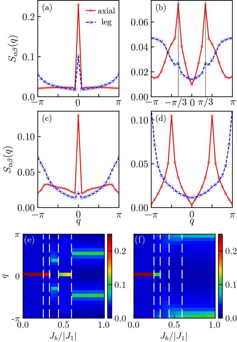
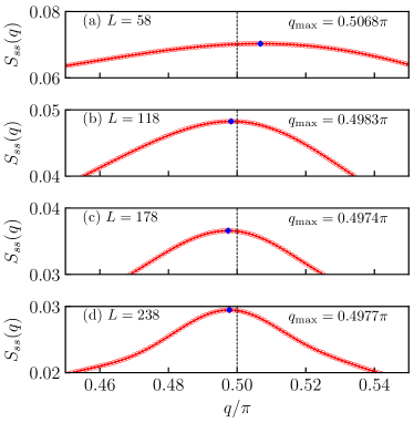
where the distance between the neighboring unit cells is taken to be unity. We here use a PBC cluster with , i.e., . In Fig. 3(a)-(d), we show the DMRG results of for the FR1 (), OS (), FR2 (), and P4 () phases. We note that due to the lattice symmetry.
In the FR1 phase [Fig. 3 (a)], both of and have a sharp peak reflecting the polarized axial and leg spins, and has an additional relatively dull peak at . This two-peak structure of is a consequence of the anomalous value of spontaneous magnetization (see Sec. IV.2).
In the OS phase [Fig. 3 (b)], has its maximum value at , which suggests a commensurate magnetic structure with a large superlattice with unit cells, i.e., 18 sites if the LRO is assumed. The dominant fluctuations in the leg-spin subsystem are noted to be AFM since is maximum at . Nevertheless, has also small shoulders at . This implies that the leg spins take part in the formation of the large superlattice structure. These are consistent with the identified OS structure (see Sec. IV.3).
In the FR2 phase [Fig. 3 (c)], the overall structures of look similar to those in the FR1 phase. The main difference is that the relative heights of and peaks are inverted. The small peak at corresponds to the weak polarization of leg spins and the larger peak at reflects the AFM fluctuations in the leg-spin subsystem. However, since the FM polarization in the axial-spin subsystem is LRO and the AFM structure in the leg-spin subsystem is not LRO as explained in the next subsection, the peak of disappears and peak of remains finite in the thermodynamic limit. This peak structure is similar to that of a FR phase in the FM-AFM delta chain [11] because of the same origin of spontaneous magnetization (see Sec. IV.4).
In the P4 phase [Fig. 3 (d)], the peaks of and are located at and , suggesting the period of magnetic structure with four and two unit cells, respectively. Since and have no common peak positions, it may be considered that the magnetic structures of axial-spin and leg-spin subsystems are essentially separated. Therefore, although the interaction between axial-spin and leg-spin subsystems is considered to be weak, it is sufficient to collapse the long-range behavior of topological string order of the leg-spin subsystem, as further discussed in Sec. IV.5. In Fig. 3(e,f) the above results are summarized as intensity plots of and with . We find that the dominant peak position is unchanged within each phase. Therefore, the periodicity would be a key factor to determine their magnetic structures.
III.3 Spin-spin correlation function
In order to obtain further insight into the nature of each phase, we examine the decay behavior of spin-spin correlation functions for each of the axial-spin and leg-spin subsystems.The spin-spin correlation function is defined by
| (5) |
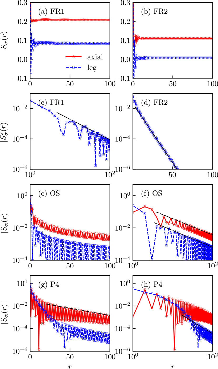
where the distance between neighboring unit cells is taken to be unity. In Fig. 4, we plot iDMRG results for the spin-spin correlation function as a function of distance . The results for and correspond to those for the axial-spin and leg-spin subsystems, respectively. Note that the spin-spin correlation functions for and coincide because of the lattice symmetry.
Fig. 4 (a) and (b) show for the FR1 and FR2 phases, respectively. We can clearly see the convergence of to a finite value, reflecting the FR nature of these phases at large enough . The converged value is equal to the spin polarization squared, i.e., and , where is the amount of spontaneous magnetization shown in Fig. 2(c). We also look at the oscillating part of spin-spin correlation function for the leg-spin subsystem, which can be extracted via
| (6) |
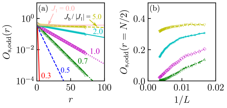
The oscillating part for the FR1 and FR2 phases are plotted in Fig. 4 (c) and (d), respectively. It is surprising that they exhibit completely different behaviors; a power-law decay for the FR1 phase and an exponential decay for the FR2 phase. This means that the leg-spin subsystem is in a gapless and a gapped ground states in the FR1 and FR2 phases, respectively. The details are explained in Sec. IV.2 and Sec. IV.4.
In Fig. 4 (e,f), the spin-spin correlation functions for the OS phase are shown. Both and exhibit power-law behaviors and decay approximately as . This clearly indicates a gapless nature of the OS state. Actually, the spinon excitation from the OS ground state is gapless as confirmed in the next subsection. The OS state has an LRO with alternating alignment of octamer singlets and nearly free axial spins. Considering the period of magnetic structure with six structural unit cells, i.e., containing 18 spins, as found by the static spin structure factor, it appears that the nearly free axial spins are antiferromagnetically coupled and form a spin-1/2 Heisenberg chain. Thus, the power-law behavior with is naively expected. Further details are given in Sec. IV.3.
In Fig. 4 (g,h), the spin-spin correlation functions for the P4 phase are shown. It is interesting that the correlation functions for the axial-spin and leg-spin subsystems have completely different behaviors. For the axial spins, exhibits an exponential decay indicating a gapped nature. In the P4 phase, all the axial spins form valence bonds as a consequence of order-by-disorder mechanism. Thus, the axial-spin subsystem is gapped, which is consistent with the exponential decay of . For the leg spins, exhibits an exponential decay at short distance and a power-law decay at long distance. In the P4 phase, the leg-spin subsystem can be mapped onto a spin-1 Heisenberg chain in the sector. Accordingly, one may expect an exponential decay of spin-spin correlation function since the Haldane-like VBS state may be the prospective ground state. This seems to be consistent with the exponential decay of at short distance. However, in fact, the Haldane-like VBS state is ’weakly’ collapsed due to the weak interaction with the axial-spin subsystem. Therefore, the behavior of shows a crossover from an exponential deecay at short distance to a power-law decay at long distance. This also means that it looks as if the Haldane-like VBS state is stabilized at short range. In the other words, the P4 state may be regarded as a pseudo-gapped state. Further details are given in Sec. IV.5 and Sec. IV.6.
III.4 Spin gap
We here examine whether a spin excitation from the ground state is gapped or gapless in each phase. To address this issue, we define a spin gap as the energy difference between the ground state and the first excited state with a flipped spin:
| (7) | ||||
| (8) |
where is the ground state energy of the system of size and the z-component of total spin . For the OS and P4 phases, the ground state is in a singlet state and we can simply take . On the other hand, a definite treatment is required for the FR phases since the ground state is macroscopically degenerate. Specifically, we set for the FR1 phase and for the FR2 phase to verify a spin excitation above their degenerate ground state. Furthermore, to avoid underestimating the gap in association with any free boundary effects, we adopt the PBC. In Fig. 5, we show the size dependence of the spin gap for the FR1 (), FR2 (), OS (), and P4 () phases. The spin gap extrapolated to the thermodynamic limit is finite only for the FR2 phase and zero for the other phases. This can be explained as follows.
In the FR1 phase, since the axial spins are fully polarized, the calculated spin gap corresponds to a gap in the spin excitation spectrum of the leg-spin subsystem. As described in Sec. IV.2, the leg-spin subsystem behaves like a critical SU(2) Heisenberg chain. Thus, the leg-spin subsystem is gapless and it is also consistent with the power-law decay of its spin-spin correlation function .
In the OS phase, our system consists of octamer singlets and residual nearly-free spins (see Sec. IV.3). The residual spins are weakly connected and form a critical SU(2) Heisenberg chain. Although a finite energy is required to excite the octamer singlet, the excitation of residual spins is gapless. A parabolic finite-size scaling of the spin gap, i.e., is a typical feature of a critical Heisenberg chain.
In the FR2 phase, the axial spins are fully polarized as in the FR1 phase. Therefore, the finite spin gap indicates a gapful nature of the leg-spin subsystem. It seems natural to assume that the leg-spin subsystem is in a Haldane-like VBS state because the translational symmetry is not broken as shown below. This is indeed a possible scenario because the leg-spin subsystem can be mapped onto an effective spin-1 Heisenberg chain in the sector. If this is the case, the finite spin gap and the exponential decay of can be reasonably explained. A simplest way to check the presence of a Haldane-like VBS state is to see the edge states of a open spin-1 chain [33]. To achieve this, we have calculated the spin gap for two kinds of open chains (data not shown). One is a simple open chain with remaining upper and lower leg spins at the open edges. The other is also an open chain but either of the upper or lower leg spins is removed at the open edges. This is equivalent to replacing spin-1 degrees of freedom by spin-1/2 degrees of freedom at the edges of a spin-1 open chain. We have found that the spin gap is zero for the former open chain and is finite for the latter open chain. The spin gap estimated with the latter open chain coincides with that estimated with PBC chain in the thermodynamic limit. This result provides a solid numerical evidence for the presence of Haldane-like VBS state.
In the P4 phase, the axial-spin and leg-spin subsystems may be considered separately as their spin-spin correlation functions show completely different behaviors [see Fig. 4 (g,h)]. As described in Sec. IV.5, the axial-spin subsystem is spontaneously dimerized and gapful while the leg-spin subsystem may be regarded as a kind of spin-1 Heisenberg chain. However, if the the leg-spin subsystem is in a Haldane-like VBS state as in the FR2 phase, the spin gap should be finite. Hence, taking into account the power-law decay of , the leg-spin subsystem seems to be in a Tomonaga-Luttinger liquid state. Although it appears to be true that a Haldane-like VBS state is stabilized in the FR2 phase, the Haldane gap () at is much smaller than that for the corresponding pure spin-1 Heisenberg chain . Thus, the Haldane-like VBS state in the FR2 phase seems not to be very stable. On the other hand, in the P4 phase, a Haldane-like VBS state is not stabilized in a strict sense, but the tendency is seen as an exponential decay of at short distance. Thus, we find it a delicate problem to identify the reason why a Haldane-like VBS state is stabilized in the FR2 phase but not stabilized in the P4 state, which is left as a future challenging issue.
IV Phases
In the previous section, based on the results of the spontaneous magnetization and magnetic period, we have shown that the ground state of our system exhibits five different phases, i.e., FM, FR1, OS, FR2, and P4, in the space. In this section, we determine the microscopic magnetic structure of each phase and reveal their origins. Especially, both the similarities and differences between the FR1 and FR2 states are elucidated in considerable detail. Furthermore, we show numerical evidences for spontaneous translational symmetry breaking, which is accompanied with valence bond formation in the OS and P4 phases. We also clarify the reason why the OS and P4 states have a gapless spin excitation in spite of the valence bond formation.
IV.1 Ferromagnetic (FM) phase
In the limit of , our system is in a trivial FM ordered ground state. With increasing , the FM state persists up to ; then, a first-order phase transition from the FM to FR1 state occurs [21]. The critical value of can be exactly estimated by the classical spin wave theory. The Fourier transform of our Hamiltonian (2) reads
| (9) |
with
| (10) |
where and . Since the system contains two kinds of spins, i.e., axial and leg spins, the dispersion is split into two branches. The minimum position of Eq. (10) changes from to at , which is consistent with the FM critical value estimated from the total spin. Then, Eq. (10) has a minimum at in the whole region of . However, as shown above, the DMRG result for the static structure factor exhibits switching among several peak positions depending on the value of . This discrepancy implies the importance of quantum effects in this system.
IV.2 Ferrimagnetic-1 (FR1) phase
With increasing , the spontaneous magnetization drops down from to at . The value of , which is maintained in the region of , indicates a commensurate FR state. We refer to this state as FR1 state.
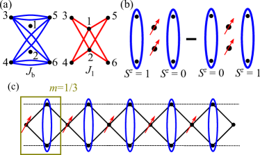
Let us then determine the magnetic structure of the FR1 phase. According to the Lieb-Schultz-Mattis (LSM) theorem [34, 35], a FR state with is allowed only when a number is an integer, where is the number of sites in magnetic unit cell. Since in the FR1 phase, needs to be a multiple of . We thus consider a 6-site periodic cluster () of our system (2) which may possibly be a minimal unit to describe the FR1 state [Fig. 6(a)]. The Hamiltonian of the 6-site cluster can be easily diagonalized and we find three ground states depending on : FM state with (), FR state with (), and singlet state with (). Obviously, the state corresponds to the FR1 state. The ground state wave function of the state is exactly written as
| (11) |
independently of , where denotes a spin state of site . The site indices are assigned in Fig. 6(a). For convenience, the magnetization direction is assumed to be along the z-axis, i.e., 5 up and 1 down spins are contained in the 6-site cluster.
We here notice that two leg spins and , i.e., two spins at sites 3 and 4 (as well as 5 and 6) in the 6-site cluster, form a spin-triplet pair, which leads to a resultant effective spin-1 site . In general, a spin-triplet pair state between sites and can be mapped onto a spin-1 degree of freedom via three states:
| (12) | |||
| (13) | |||
| (14) |
for , , and states, respectively. Using this transformation, Eq. (11) can be expressed as
| (15) |
Thus, the ground state wave function of state can be separated into two parts: (I) the fully polarized axial spins, i.e., , and (II) an antisymmetric combination of two spin states of two effective spin-1’s. It is striking that the state is completely projected out in part (II). Since all the leg spins are ferromagnetically coupled to the polarized axial spins , the FM interaction behaves like an external magnetic field on the leg spins, or like a uniaxial single-ion-type anisotropy to enhance the magnetization of each effective spin-1 site [36]. By considering replacements and , we can easily recognize that the part (II) has the same form as a spin-singlet pair state in spin- system. Accordingly, the two spin-1 degrees of freedom, each of which is exactly reduced to a SU(2) symmetry with two states and , are antiferromagnetically coupled. The state of part (II) is illustrated in Fig. 6(b).
As a result, if the system size is extended to infinity, the leg spins form a spin-1 AFM Heisenberg chain with the reduced spin space to a SU(2) symmetry. And, the axial spins are nearly fully polarized as also confirmed numerically in Sec. III.1. If all the axial spins are assumed to be fully polarized, the effective spin-1 chain needs to contain the same numbers of and sites to maintain . This is a natural consequence of the fact that the energy gain from the exchange processes is maximized when the numbers of and sites are equal, just as the SU(2) Heisenberg chain has the lowest energy at . Therefore, this effective spin-1 chain behaves like a critical SU(2) chain with the reduced Hilbert space of a spin from to dimensional. Accordingly, there is no magnetic order accompanied by a translational symmetry breaking with alternating sites of and . This is consistent with the power-law decay of the spin-spin correlation function for the leg-spin subsystem .
Although we assumed a magnetic unit cell with to fulfill the LSM theorem, it is not the case that the FR1 state obeys the LSM theorem because the magnetic unit cell is ill-defined in the FR1 phase.
IV.3 Octamer-singlet (OS) phase
A narrow spin-singlet () phase appearing for is sandwiched between two FR phases. It means that this state is not a consequence of simple melting of FR order by AFM but attributed to a kind of LRO stabilization. However, the possibility of magnetic order can be ruled out by the power-law decay of the spin-spin correlations and . Then, the most likely LRO is a valence bond formation due to the order-by-disorder mechanism. The representatives of such valence bond formation are spontaneous dimerization orders in the AFM-AFM - chain [3] and in the FM-AFM - chain [37]. In these systems the ground state is characterized as a valence bond solid (VBS) state with an exponential decay of spin-spin correlation and a finite gap in the spin excitation. And yet, in our system, the spin-spin correlation decays in power law and the first excitation is gapless. That is to say, although our system at is in an LRO state associated with valence bond formation, it is not a simple VBS state. In other wards, the system is not fully filled with the valence bonds.
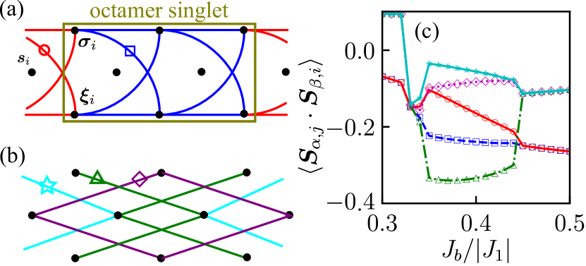
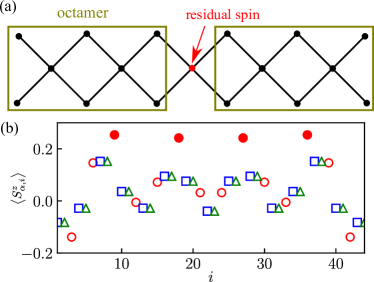
To determine the valence bond structure, we calculate the real-space distribution of spin-spin correlation functions . In Fig. 7(c) we plot the iDMRG results for as a function of . The symbols and colors correspond to bonds shown in Fig. 7(a) and (b). Although the bonds denoted by red circle and blue square are geometrically equivalent, the correlations between these bonds are split at . Similarly, the correlations among the bonds denoted by green triangle, purple diamond, and cyan star are also split in the same region. This result clearly indicates that the translational symmetry is spontaneously broken with the tripled unit cell, i.e., a 3-period magnetic unit cell containing 9 spins. This situation may be reasonably explained by assuming that 8 spins out of the 9 spins in the magnetic unit cell, surrounded by a yellow box in Fig. 7 (a), form an OS state. In fact, we have confirmed that the isolated octamer has a stable singlet ground state with a finite excitation gap. The excitation gap has its maximum value around . This means that the frustration of exchange interactions can indeed be relieved by forming the octamer-singlet units. The details are discussed in Appendix A.
Nevertheless, there are extra axial spins between the octamer units. The extra axial spin thus appears in every three structural unit cells. Considering the sharp peaks of at , it appears that the extra axial spins are antiferromagnetically connected and an AFM Heisenberg chain is formed. Since the Heisenberg chain is critical, the whole system should be gapless in spite of gapped octamer singlets. It is consistent with the power-law decay of the spin-spin correlations. Thus, we conclude that the region is identified as the octamer-singlet phase. The phase transitions between the OS and two FR phases are of the first order because these phases have completely different symmetries.
IV.4 Ferrimagnetic-2 (FR2) phase
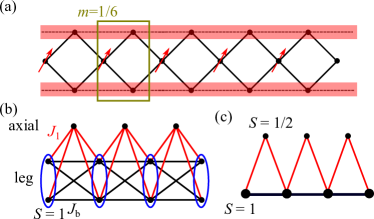
Another FR phase different from the FR1 phase appears at , where the total spin is . This phase is referred to as the FR2 phase. In the FR2 phase, the axial spins are nearly fully polarlized and the leg spins are only weakly polarlized (see Fig. 2). The schematic magnetic structure of the FR2 state is sketched in Fig. 8 (a). Here, we are aware of a spin model exhibiting a similar FR state. That is the spin-1/2 FM-AFM delta chain which consists of nearly-fully polarlized spin-1/2 apical spins and weakly polarlized spin-1/2 basal spins in its FR phase (we refer to this phase as “delta-FR” phase hereafter) [32, 38]. Interestingly, this delta-FR order is not associated with geometrical symmetry breaking; instead, the global spin-rotational symmetry is broken via the order-by-disorder mechanism [11]. Actually, in the FR2 phase both of the axial-axial and leg-leg spin-spin correlations converge to finite positive values at the long distance [see Fig. 4(b)]. This indicates a global spin-rotational symmetry breaking without any translational symmetry breaking. Moreover, the kagome chain can be regarded as a FM-AFM delta chain if we assume the resultant two leg spins to form [see Fig. 8 (b) and (c)]. Namely, the basal spins are not but . It has been confirmed that this mapping of leg chains into a single spin-1 Heisenberg chain is exact in the limit of [12]. Nevertheless, since the FM fluctuations between the apical and basal spins are essential to stabilize the FR state, the FR mechanism associated with the global spin-rotational symmetry breaking should work even in the the case of spin-1 basal chain. Thus, we may expect that the FR2 state is induced by the same order-by-disorder mechanism as the delta-FR state.
Although the origin of the FR2 and delta-FR states are identical, there is a discrepancy in the parameter range between them. While the delta-FR phase maintains at the large limit of AFM interaction between the basal spins, the FR2 phase disappears only around . We can think of three possible reasons for this discrepancy: First, the basal chain is more classical than the one so that the FM fluctuations with the apical spins are more suppressed. Secondly, the weak FM order in the effective basal chain may be affected by the presence of pseudo-Haldane order (see Sec. IV.6). Third, even though in hindsight, the other order-by-disorder phase, called as the period-4 phase, appears at the larger AFM interaction (see also Sec. IV.5).
As mentioned above, the translational symmetry is not broken in the FR2 phase. Accordingly, the magnetic unit cell is the same as the original structural unit, i.e., . In that sense, one may say that the LSM condition for a FR stabilization is fulfilled. From this standpoint, the FR2 phase is different from the FR1 phase which is non-LM FR one. However, the two FR phases are similar in that the axial spins are nearly fully polarized. This fact provides us with another insight that the fractionally quantized spin state of the effective chain, consisting of the leg spins, is changed as , , and in the FM, FR1, and FR2 phases, respectively. It can be interpreted as follows: The leg spins feel the FM correlations with the polarized axial spins like an external magnetic field. When the AFM interaction between leg spins, i.e., , is small, the leg spins have full magnetization, leading to the FM phase. Then, the magnetization of leg spins are reduced with increasing . Interestingly, the change of magnetization is not continuous but quantized. Nevertheless, it is consistent with the Marshall-Lieb-Mattis theorem which prohibits a “halfway” magnetization [39, 17]. If the axial spins are directly coupled by AFM interaction, a continuous change of magnetization may be allowed as a consequence of the competition between the spin polarizations and a critical Tomonaga-Luttinger–liquid behavior [20, 11].
Related to this issue, it would be informative to understand the reason why the FR2-like state does not exist as a ground state of the 6-site cluster discussed in Sec. IV.2 [see Fig. 6(a)]. Basically, the energy gain from the FM fluctuations between axial and leg spins are essential to stabilize a FR state. In the FR1 state, such FM fluctuations are simply accomplished because the system consists of axial spins with and leg spins with . This state can be clearly expressed even within the 6-site cluster. On the other hand, the leg spins need to be spontaneously polarized to stabilize the FR2 state. To achieve this, the FM axial-leg fluctuations favoring must exceed the competing AFM intra-leg exchange fluctuations favoring . However, the AFM exchange fluctuations are always dominant with a short chain so that the FR2 state cannot exist as a ground state of the 6-site cluster. This is one of the typical finite-size effects and a certain chain length is required to obtain the FR2 ground state. A similar discussion was given in the spin-1/2 delta chain [11].
IV.5 period-4 (P4) phase
At , the system goes again into an phase from the FR2 phase. As mentioned above, a fourfold magnetic structure is indicated by the sharp peaks of at for the leg chains and at for the axial chain. One may naively imagine that this state is a spin liquid due to melting of FR2 order by AFM . However, given the exponential decay of spin-spin correlations between the axial spins [Fig. 4(e,f)], we find it not to be a simple spin liquid but a ‘gapped’ state in association with valence bond formation. Nevertheless, we note that the first excitation above the ground state is in fact gapless as shown in Sec. III.4. Although this is seemingly puzzling, we may solve it by looking at our system divided into two subsystems, namely, a system of axial spins and that of leg spins. In fact, both of the spin structure factor [Fig. 3(d)] and spin-spin correlations [Fig. 4(e,f)] behave quite differently between the axial-spin and leg-spin subsystems.
Let us then consider the effective models of the two subsystems. As already mentioned above, a spin-1 AFM Heisenberg chain provides a good approximation of the leg-spin subsystem. The maximum value of at [Fig. 3(f)] reflects the dominant AFM fluctuation. It is known that the ground state of spin-1 AFM Heisenberg chain is a gapped state called Haldane VBS [40] or Affleck-Kennedy-Lieb-Tasaki [41] state. In fact, the exponential decay of at short distance [Fig. 4(e)] exhibits a signature of the gapped feature. However, it turns to a power-law decay at long distance [Fig. 4(f)] because the Haldane VBS state is not a perfect long-range order due to the interaction with the axial-spin subsystem. As shown in Fig. 4(e) and (f), the crossover from exponential to power-law behaviors occurs around at . With increasing the range of exponential decay, i.e., , increases and the Haldane VBS state is recovered in the limit of . This point will be further discussed in the next subsection.
On the other hand, a possible effective model for the axial-spin subsystem is a frustrated FM-AFM Heisenberg chain with nearest-neighbor FM coupling and next-nearest-neighbor AFM coupling [42]. The ground state of this frustrated chain is either an FM state at or an incommensurate spiral VBS state with valence bond formation between third-neighbor sites at [37]. Let us estimate the effective exchange parameters within perturbation theory. Assuming an AFM alignment of leg-spin subsystem as an unperturbed state, the second- and third-order perturbations give
| (16) |
[see Fig. 9(a)]. This leads to . Hence, the range of for the P4 phase corresponds to the incommensurate spiral VBS phase of frustrated FM-AFM Heisenberg chain. Meanwhile, as shown in Fig. 3(d), a commensurate peak of at has been obtained for . In fact, the propagation number is for () [43]. Thus, the PBC cluster used for Fig. 3(d) does not have high enough resolution to detect such a tiny deviation from . In Appendix B, we confirm that the actual propagation number in the P4 phase is slightly less than .
As discussed above, the ground state of axial-spin subsystem in the P4 phase corresponds to an incommensurate spiral VBS state of frustrated FM-AFM Heisenberg chain. We then investigate whether valence bonds are actually formed in the P4 state. To identify the possible structure of valence bond formation, the short-range spin-spin correlations for the bonds denoted in Fig. 9(b) are calculated. The iDMRG results for short-range spin-spin correlations are plotted as a function of in Fig. 9(c). We find that the spin-spin correlation between next-nearest-neighbor axial spins is uniform in the FR2 phase (), which largely splits into two values [denoted by red circles and blue squares in Fig. 9(c)] as soon as the system goes into the P4 phase (). This obviously means that the axial-spin subsystem is spontaneously dimerized, where the valence bond is formed between next-nearest-neighbor axial spins coupled by in the effective model. This is different from the fact that a valence bond is formed between third-neighbor sites in the frustrated FM-AFM Heisenberg chain. In order to see the dimerzation strength, we define the dimerization order parameter as
| (17) |
The iDMRG result for is plotted as a function of in Fig. 9(c). An abrupt occurrence of at the boundary between FR2 and P4 phases indicates a first-order phase transition, which is consistent with the discontinuous changes of the total spin at the phase boundary. With increasing , the dimerization order parameter decreases from its maximum at and saturate at some value in the limit of . This can be interpreted in terms of the frustration ratio of the effective model, i.e., of the frustrated FM-AFM Heisenberg chain. We estimate at It is known that the frustration strength is maximum around in the frustrated FM-AFM Heisenberg chain [43]. Since the dimerization order is a consequence of order by disorder, this result is consistent with the fact that the dimerization order parameter is maximum around . Besides, the approach of frustration ratio to at leads to the saturation of dimer order parameter. However, the limit of is not adiabatically connected to a point. The point is singular and the dimer order no longer exists because the axial-spin subsystem is just a group of free spins. This means that the inclusion of finite gives non-perturbative effects in the axial-spin subsystem. The existence of such singularity may also be expected in the AFM-AFM Kagome-like chain [28], which needs to be studied in the future. In the next subsection, we will give a further discussion on this issue from the viewpoint of the string order parameter.
As described above, our system can be considered as the direct product of gapless leg-spin subsystem and gapped axial-spin subsystem in the P4 phase. This decoupling of our system is further supported by the fact that the spin-spin correlation between axial and leg spins is very small, only of the order of . Accordingly, we can routinely understand the completely different behaviors of spin-spin correlation functions between the axial-spin and leg-spin subsystems, namely, the power-law decay of [Fig. 4(f)] and the exponential decay of [Fig. 4(e)] at long distance. Note that the whole system is gapless as shown in Sec. III.4.
IV.6 Pseudo-Haldane state
At , our system is completely decomposed into the leg-spin subsystem and free axial spins. The leg-spin subsystem is equivalent to the so-called diagonal ladder with uniform exchange couplings. Although the diagonal ladder has been intensively studied in the context of columnar-dimer phase, no positive numerical evidence for a dimerized state has so far been found in the previous studies [44, 45, 46, 47]. This is consistent with our results and we have further confirmed that even the inclusion of finite FM does not derive any dimerized state.
Another interesting issue from the viewpoint of topological order is the hidden Haldane VBS order [48]. The diagonal ladder with uniform exchange couplings, i.e, our leg-spin subsystem at , is exactly mapped onto a spin-1 Heisenberg chain
| (18) |
Therefore, the appearance of Haldane VBS order as a hidden symmetry breaking is naturally expected. This order can be revealed by a string order parameter defined through a nonlocal unitary transformation [48, 49, 50, 51]. Let us then consider what happens when FM is switched on. To study this, we calculate the -component of a nonlocal string correlation function
| (19) |
The string order parameter is defined as a value of at long-distance limit . In Fig. 10 we show the iDMRG and DMRG results for the string correlation function as a function of distance for several values of FM . At , we can clearly confirm a long-range hidden VBS order with a convergence to at long distance, which is consistent with the previous study [52]. Surprisingly, just by introducing small (), the correlation function turns to an exponential decay, although its correlation length seems to be still very large. With further increasing , the decay of becomes faster, keeping its exponential behavior. Since the point is singular for the axial-spin subsystem, it may be a good guess that the hidden Haldane VBS order in the leg-spin subsystem no longer exists at any finite . However, more precise iDMRG analysis of at semi-infinite distance, e.g., , is necessary to confirm it [53].
In Fig. 10(b), a finite-size scaling of is shown. We recognize that the correlation length of is maintained to be relatively long.at (). The correlation length may roughly be estimated from the change in slope of vs. . For example, let us see the case of : The slope of vs. looks almost linear at , which indicates a short-range stability of the hidden VBS order. At , the value of goes toward zero with decreasing , which suggests a collapse of the long-range hidden VBS order. From the changing point of slope, the correlation length is roughly estimated as . It is indeed reasonable that this correlation length agrees well to the crossover distance of the spin-spin correlation functions , where the change in from exponential to power-law behaviors occurs at [see Fig. 4(e) and Sec. IV.5]. This means that it looks as if a hidden VBS order is stabilized at , although the long-range order is actually collapsed by finite . This unique feature makes our analysis to identify the string order parameter difficult and the use of iDMRG is necessarily required. A similar difficulty is seen, for example, in the study of XY phase of spin-1 Heisenberg chain [54]. This issue also reminds us of a different behavior in a similar system; the AFM-AFM delta chain consisting of spin-1/2 basal and spin-1 apical sites [55]. In this system, the Haldane VBS phase survives for small apical-basal interactions. To find the reason why the different behaviors occur is left for the future.
IV.7 Relevance to experiments
Finally, let us comment on the relevance of our results to the experimental observations for Ba3Cu3In4O12 and Ba3Cu3Sc4O12. These materials have a similar field–temperature (–) phase diagram [25, 24, 26]: At , these materials exhibit a 3D AFM order indicated by a sharp peak of the magnetic susceptibility and a jump of the specific heat at low . It would be originated from weak AFM interchain couplings between the Kagome-like chains. With increasing , these systems undergo a phase transition from the AFM to spin-flop phase, and then to a fully polarized ferromagnetic phase. Of particular interest is that two-step phase transitions occur in the spin-flop phase at magnetic fields of T and T in Ba3Cu3In4O12 [26]. At the phase transitions, the experimental magnetization is and for T and T, respectively. These magnetization values are close to those of the FR2 phase () and of the FR1 phase (). Thus, the two phase transitions in the spin-flop phase may correspond to the instabilities of the two kinds of FR phase in the kagome-like chain, namely, the difference of magnetic susceptibility between the apical and leg spins. Further investigation on the - phase diagram is beyond the scope of this paper but is a fascinating open issue to be addressed in the future.
V summary
Using the DMRG-based techniques, we studied the spin-1/2 FM-AFM Kagome-like ladder with FM coupling between the axial and leg spins and AFM coupling between the leg spins . Based on the numerical calculations of the total spin, static structure factor, spin-spin correlation functions, spin gap, dimer order parameter, and string order parameter, we found five different phases in the ground state, depending on , as summarized in Fig. 1(c): FM (), FR1 (), OS (), FR2 (), and P4 () phases.
The FM, FR1, and FR2 phases are characterized by the spontaneous spin-rotational symmetry breaking. The average magnetization per site is , , and in the FM, FR1, and FR2 phases, respectively. A (nearly) fully polarization of the axial spins is a common structure of these three phases; the difference is attributed to a fractional quantization of the leg-spin magnetization. Since the leg-spin subsystem can be mapped onto an effective spin-1 Heisenberg chain with spin-1 degrees of freedom formed by the upper and lower leg spins, the issue comes to the three-step magnetization for the effective spin-1 chain. First, in the FM phase, the effective spin-1 chain is trivially in a full polarization due to the dominant FM interactions. Second, in the FR1 phase, the magnetization per site in the effective spin-1 chain is although only either or is generally allowed in a stable ground state. What happens is that an unusual critical SU(2) state with the reduced Hilbert space of a spin from to dimensional is achieved to maximize the energy gain from both the exchange processes and the FM correlations with the axial spins. Third, in the FR2 phase, the magnetization in the effective spin-1 chain should essentially be although it is actually small finite because of the spin-rotational symmetry breaking. It is surprising that, nevertheless, the Haldane-like VBS state is present in the effective spin-1 chain. In fact, this small magnetization is a consequence of order by disorder to stabilize the FR2 state, where the global spin-rotational symmetry is broken, in order to lower the energy by the FM fluctuation between the axial-spin and the leg-spin subsystems. This is the same order-by-disorder mechanism as for an FR state in the spin-1/2 FM-AFM delta chain [11]. Thus, an anomalous fractional quantization in a spin-1 Heisenberg chain as an effective model for the leg-spin subsystem is a key factor to understand the three kinds of polarized phases in the spin-1/2 Kagome-like ladder.
The remaining two phases are spin-singlet phases. One of them is the OS phase, which is sandwiched between the FR1 and FR2 phases. It implies that this phase is not a consequence of simple melting of FR state but a kind of spontaneous valence bond formation from the order-by-disorder mechanism. We performed a detailed analysis of the short-range spin-spin correlations and identified a long-range order with alternating alignment of octamer singlets and nearly-free axial spins. The nearly-free axial spins are weakly antiferromagnetically connected and a critical SU(2) chain is formed. Hence, this state is gapless and also consistent with the period of magnetic structure with six unit cells, i.e., containing 18 spins, indicated by sharp peaks at in the static spin structure factor for the axial-spin subsystem. We should note that this AFM correlation is not LRO. The other spin-singlet phase is the P4 phase characterized by the magnetic superstructure with a period of four structural unit cells. This phase appearing at large AFM coupling may be accounted for by the melting of FR state. Still, the magnetic structure is not very simple. The axial-spin subsystem is gapped with spontaneous dimerization. The leg-spin subsystem behaves like a spin-1 Heisenberg chain at short distance and like a critical chain at long distance. Accordingly, the string correlation function exhibits an exponential decay but with a long correlation length. The string order is recovered in the limit of large . Thus, in the OS and P4 phases, we detected the coexistence of valence bond structure and gapless chain. Although this may be emerged through the order-by-disorder mechanism, there can be few examples of such a coexistence.
We also discussed the relevance of the spin-1/2 FM-AFM Kagome ladder to the experimental observations of a series of field-induced spin-flop transitions in Ba3Cu3In4O12 and Ba3Cu3Sc4O12. Since the magnetization values at the two spin-flop transitions are close to those of the FR2 phase () and of the FR1 phase (). Thus, the two phase transitions in the spin-flop phase may correspond to the instabilities of the two kinds of FR phase. Further investigations of the spin-1/2 Kagome-like ladder on the - parameter space are highly desired in the future.
ACKNOWLEDGEMENTS
We thank Ulrike Nitzsche for technical support. This work was supported by Grants-in-Aid for Scientific Research from JSPS (Projects Nos. JP17K05530, JP19J10805, and JP20H01849) and by SFB 1143 of the Deutsche Forschungsgemeinschaft (Project-id 247310070). T.Y. acknowledges financial support from the JSPS Research Fellowship for Young Scientists. Some part of numerical computations were carried out on XC40 at YITP in Kyoto University.
Appendix A Spin polarization in the octamerized phase
In the main text, we have argued that our system (2) is in the octamer-singlet ground state at . The stabilization of this state is attributed to a spontaneous octamerization of the system with translational symmetry breaking. More specifically, as sown in Fig. 11(a) an octamer singlet and a nearly free spin are aligned alternately. Here, in order to further confirm the octamerization, we give another numerical evidence for the formation of octamer singlets with the use of the difference of magnetic susceptibility between the octamer singlet and nearly free spin. We apply the open boundary conditions and keep the total number of site equal to , where is an integer value, to be consistent with the octamer-singlet ground state. With this setup, there are nearly free spins. If one spin is flipped in the octamer-singlet ground state, the nearly free spin out of 9 spins should be firstly polarized.
In Fig. 11(b), we show an expectation value of the z-component of spin operator at , where the system size is set to be with . As we intuitively expected, a substantial polarization is seen at four sites corresponding to the nearly free spins (red filled circles); the other spins forming the octamer singlets are much less polarized (open symbols). This result supports the octamerization of our system in the intermediate AFM coupling regime .
We note that the nearly free spins are effectively antiferromagnetically coupled with each other since the period of magnetic modulation is twelve sites because of sharp peaks of the apical-spin structure factor at . Nevertheless, the AFM chain consisting of nearly free spins is critical, which is consistent with the gapless behaviors shown in the main text.
Appendix B Excitation gap of the isolated octamer singlet
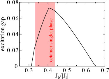
In the main text, we have claimed a spontaneous formation of octamer singlets through the order-by-disorder mechanism at . However, in fact, it is a nontrivial question whether each octamer has a gapped excitation from its singlet ground state. To confirm this, we calculate the lowest energy of isolated octamer in the and sectors. We then find that the energy for sector is indeed lower than that for the sector at . This indicates that the isolated octamer has a singlet ground state in this range. In Fig. 12, the energy difference between the ground state and excited state is plotted as a function of , which corresponds to an excitation gap of the isolated octamer. The excitation gap has a maximum around . In the octamer-singlet phase of the kagome-like chain, the order-by-disorder mechanism works to lower the frustration energy by spontaneously forming octamer singlets. Thus, it appears that the excitation energy directly reflects the stability of octamer-singlet phase. It is quite reasonable that the octamer-singlet phase exists in a region, where the excitation gap of isolated octamer is maximized.
Appendix C Nearly commensurate spin structure in the period-4 phase
The period-4 state may be characterized by a commensurate peak of at . This means that the magnetic period is four structural unit cells, containing axial spins. On the other hand, as described in the main text, the apical-spin subsystem can be effectively mapped onto the so-called ferromagnetic-antiferromagnetic - chain in the period-4 phase at . In the main text, and are referred to as and , respectively. From the perturbative analysis [Eq. (16)], the range of frustration ratio is estimated to be for . Although the propagation number is known to be very close to in this range, a true commensurate modulation with is achieved only in the limit of [56]. If this is the case, the precise peak position of in the period-4 phase could be slightly shifted from . To check this, we calculate the static spin structure factor [Eq. (4)] with open chains. The use of open boundary conditions enables us to tune the propagation number continuously as a function of in the situation of ill-defined momenta. In Fig. 13, the DMRG results of static structure factor for the axial spins in the kagome-like chain at are shown. Note that the parameter corresponds to in the effective - chain. We can see that the peak position is obviously shifted from . Although we have not performed the finite-size scaling analysis, the propagation number seems to converge to in the thermodynamic limit . It is also convincing that this value agrees very well with propagation number for in the - chain [43].
References
- Diep [2013] H. T. Diep, Frustrated Spin Systems, 2nd ed. (WORLD SCIENTIFIC, 2013).
- Villain et al. [1980] J. Villain, R. Bidaux, J.-P. Carton, and R. Conte, Order as an effect of disorder, J. Phys. (France) 41, 1263 (1980).
- Majumdar and Ghosh [1969] C. K. Majumdar and D. K. Ghosh, On Next‐Nearest‐Neighbor Interaction in Linear Chain. I, Journal of Mathematical Physics 10, 1388 (1969).
- Koga and Kawakami [2000] A. Koga and N. Kawakami, Quantum phase transitions in the shastry-sutherland model for , Phys. Rev. Lett. 84, 4461 (2000).
- Ganesh et al. [2013] R. Ganesh, J. van den Brink, and S. Nishimoto, Deconfined criticality in the frustrated heisenberg honeycomb antiferromagnet, Phys. Rev. Lett. 110, 127203 (2013).
- Zhu et al. [2013] Z. Zhu, D. A. Huse, and S. R. White, Weak plaquette valence bond order in the honeycomb heisenberg model, Phys. Rev. Lett. 110, 127205 (2013).
- Jolicoeur et al. [1990] T. Jolicoeur, E. Dagotto, E. Gagliano, and S. Bacci, Ground-state properties of the s=1/2 heisenberg antiferromagnet on a triangular lattice, Phys. Rev. B 42, 4800 (1990).
- Reimers and Berlinsky [1993] J. N. Reimers and A. J. Berlinsky, Order by disorder in the classical heisenberg kagomé antiferromagnet, Phys. Rev. B 48, 9539 (1993).
- Bramwell et al. [1994] S. T. Bramwell, M. J. P. Gingras, and J. N. Reimers, Order by disorder in an anisotropic pyrochlore lattice antiferromagnet, Journal of Applied Physics 75, 5523 (1994), https://doi.org/10.1063/1.355676 .
- Dmitriev and Ya Krivnov [2016] D. V. Dmitriev and V. Ya Krivnov, Ferrimagnetism in delta chain with anisotropic ferromagnetic and antiferromagnetic interactions, Journal of Physics: Condensed Matter 28, 506002 (2016).
- Yamaguchi et al. [2020] T. Yamaguchi, S.-L. Drechsler, Y. Ohta, and S. Nishimoto, Variety of order-by-disorder phases in the asymmetric - zigzag ladder: From the delta chain to the - chain, Phys. Rev. B 101, 104407 (2020).
- Kim et al. [2000] E. H. Kim, G. Fáth, J. Sólyom, and D. J. Scalapino, Phase transitions between topologically distinct gapped phases in isotropic spin ladders, Phys. Rev. B 62, 14965 (2000).
- Yamashita et al. [2010] M. Yamashita, N. Nakata, Y. Senshu, M. Nagata, H. M. Yamamoto, R. Kato, T. Shibauchi, and Y. Matsuda, Highly mobile gapless excitations in a two-dimensional candidate quantum spin liquid, Science 328, 1246 (2010).
- Jiang et al. [2012] H.-C. Jiang, Z. Wang, and L. Balents, Identifying topological order by entanglement entropy, Nature Physics 8, 902 (2012).
- Han et al. [2012] T.-H. Han, J. S. Helton, S. Chu, D. G. Nocera, J. A. Rodriguez-Rivera, C. Broholm, and Y. S. Lee, Fractionalized excitations in the spin-liquid state of a kagome-lattice antiferromagnet, Nature 492, 406 (2012).
- Banerjee et al. [2016] A. Banerjee, C. A. Bridges, J.-Q. Yan, A. A. Aczel, L. Li, M. B. Stone, G. E. Granroth, M. D. Lumsden, Y. Yiu, J. Knolle, S. Bhattacharjee, D. L. Kovrizhin, R. Moessner, D. A. Tennant, D. G. Mandrus, and S. E. Nagler, Proximate Kitaev quantum spin liquid behaviour in a honeycomb magnet, Nature Materials 15, 733 (2016).
- Lieb and Mattis [1962] E. Lieb and D. Mattis, Ordering Energy Levels of Interacting Spin Systems, Journal of Mathematical Physics 3, 749 (1962).
- Ivanov and Richter [2004] N. B. Ivanov and J. Richter, Phase diagram of a frustrated mixed-spin ladder with diagonal exchange bonds, Phys. Rev. B 69, 214420 (2004).
- Hida and Takano [2008] K. Hida and K. Takano, Frustration-induced quantum phases in mixed spin chain with frustrated side chains, Phys. Rev. B 78, 064407 (2008).
- Furuya and Giamarchi [2014] S. C. Furuya and T. Giamarchi, Spontaneously magnetized Tomonaga-Luttinger liquid in frustrated quantum antiferromagnets, Phys. Rev. B 89, 205131 (2014).
- Dmitriev and Krivnov [2017] D. V. Dmitriev and V. Y. Krivnov, Kagome-like chains with anisotropic ferromagnetic and antiferromagnetic interactions, J. Phys. Condens. Matter 29, 215801 (2017).
- Koteswararao et al. [2012] B. Koteswararao, A. V. Mahajan, F. Bert, P. Mendels, J. Chakraborty, V. Singh, I. Dasgupta, S. Rayaprol, V. Siruguri, A. Hoser, and S. D. Kaushik, Magnetic behavior of Ba3Cu3Sc4O12, J. Phys.: Condens. Matter 24, 236001 (2012).
- Badrtdinov et al. [2016] D. I. Badrtdinov, O. S. Volkova, A. A. Tsirlin, I. V. Solovyev, A. N. Vasiliev, and V. V. Mazurenko, Hybridization and spin-orbit coupling effects in the quasi-one-dimensional spin- magnet , Phys. Rev. B 94, 054435 (2016).
- Dutton et al. [2012] S. E. Dutton, M. Kumar, Z. G. Soos, C. L. Broholm, and R. J. Cava, Dominant ferromagnetism in the spin-1/2 half-twist ladder 334 compounds, Ba3Cu3In4O12and Ba3Cu3Sc4O12, J. Phys.: Condens. Matter 24, 166001 (2012).
- Kumar et al. [2013] M. Kumar, S. E. Dutton, R. J. Cava, and Z. G. Soos, Spin-flop and antiferromagnetic phases of the ferromagnetic half-twist ladder compounds Ba3Cu3In4O12and Ba3Cu3Sc4O12, J. Phys.: Condens. Matter 25, 136004 (2013).
- Volkova et al. [2012] O. S. Volkova, I. S. Maslova, R. Klingeler, M. Abdel-Hafiez, Y. C. Arango, A. U. B. Wolter, V. Kataev, B. Buchner, and A. N. Vasiliev, Orthogonal spin arrangement as possible ground state of three-dimensional shastry-sutherland network in ba3cu3in4o12, Phys. Rev. B 85, 104420 (2012).
- Waldtmann et al. [2000] C. Waldtmann, H. Kreutzmann, U. Schollwöck, K. Maisinger, and H.-U. Everts, Ground states and excitations of a one-dimensional kagom\’e-like antiferromagnet, Phys. Rev. B 62, 9472 (2000).
- M-Aghaei et al. [2018] A. M-Aghaei, B. Bauer, K. Shtengel, and R. V. Mishmash, Signatures of gapless fermionic spinons on a strip of the kagome Heisenberg antiferromagnet, Phys. Rev. B 98, 054430 (2018).
- [29] https://itensor.org/.
- McCulloch [2008] I. P. McCulloch, Infinite size density matrix renormalization group, revisited, (2008), arXiv:0804.2509 .
- Schollwöck [2011] U. Schollwöck, The density-matrix renormalization group in the age of matrix product states, Annals of Physics 326, 96 (2011).
- Tonegawa and Kaburagi [2004] T. Tonegawa and M. Kaburagi, Ground-state properties of an S=12-chain with ferro- and antiferromagnetic interactions, Journal of Magnetism and Magnetic Materials 272-276, 898 (2004).
- Kennedy [1990] T. Kennedy, Exact diagonalisations of open spin-1 chains, Journal of Physics: Condensed Matter 2, 5737 (1990).
- Lieb et al. [1961] E. Lieb, T. Schultz, and D. Mattis, Two soluble models of an antiferromagnetic chain, Annals of Physics 16, 407 (1961).
- Affleck and Lieb [1986] I. Affleck and E. H. Lieb, A proof of part of haldane’s conjecture on spin chains, in Condensed Matter Physics and Exactly Soluble Models (Springer, 1986) pp. 235–247.
- Botet et al. [1983] R. Botet, R. Jullien, and M. Kolb, Finite-size-scaling study of the spin-1 heisenberg-ising chain with uniaxial anisotropy, Phys. Rev. B 28, 3914 (1983).
- Agrapidis et al. [2019] C. E. Agrapidis, S.-L. Drechsler, J. van den Brink, and S. Nishimoto, Coexistence of valence-bond formation and topological order in the Frustrated Ferromagnetic $J_1$-$J_2$ Chain, SciPost Physics 6, 019 (2019).
- Krivnov et al. [2014] V. Y. Krivnov, D. V. Dmitriev, S. Nishimoto, S.-L. Drechsler, and J. Richter, Delta chain with ferromagnetic and antiferromagnetic interactions at the critical point, Phys. Rev. B 90, 10.1103/PhysRevB.90.014441 (2014).
- Marshall [1955] W. Marshall, Antiferromagnetism, Proceedings of the Royal Society of London. Series A, Mathematical and Physical Sciences 232, 48 (1955).
- Haldane [1983] F. Haldane, Continuum dynamics of the 1-d heisenberg antiferromagnet: Identification with the o(3) nonlinear sigma model, Physics Letters A 93, 464 (1983).
- Affleck et al. [1987] I. Affleck, T. Kennedy, E. H. Lieb, and H. Tasaki, Rigorous results on valence-bond ground states in antiferromagnets, Phys. Rev. Lett. 59, 799 (1987).
- Bader and Schilling [1979] H. P. Bader and R. Schilling, Conditions for a ferromagnetic ground state of heisenberg hamiltonians, Phys. Rev. B 19, 3556 (1979).
- Nishimoto et al. [2012] S. Nishimoto, S.-L. Drechsler, R. Kuzian, J. Richter, J. Málek, M. Schmitt, J. van den Brink, and H. Rosner, The strength of frustration and quantum fluctuations in LiVCuO 4, EPL (Europhysics Letters) 98, 37007 (2012).
- Allen et al. [2000] D. Allen, F. H. L. Essler, and A. A. Nersesyan, Fate of spinons in spontaneously dimerized spin- ladders, Phys. Rev. B 61, 8871 (2000).
- Starykh and Balents [2004] O. A. Starykh and L. Balents, Dimerized Phase and Transitions in a Spatially Anisotropic Square Lattice Antiferromagnet, Phys. Rev. Lett. 93, 127202 (2004).
- Hung et al. [2006] H.-H. Hung, C.-D. Gong, Y.-C. Chen, and M.-F. Yang, Search for quantum dimer phases and transitions in a frustrated spin ladder, Phys. Rev. B 73, 224433 (2006).
- Barcza et al. [2012] G. Barcza, Ö. Legeza, R. M. Noack, and J. Sólyom, Dimerized phase in the cross-coupled antiferromagnetic spin ladder, Phys. Rev. B 86, 075133 (2012).
- den Nijs and Rommelse [1989] M. den Nijs and K. Rommelse, Preroughening transitions in crystal surfaces and valence-bond phases in quantum spin chains, Phys. Rev. B 40, 4709 (1989).
- Kennedy and Tasaki [1992a] T. Kennedy and H. Tasaki, Hidden symmetry breaking and the haldane phase in s= 1 quantum spin chains, Communications in mathematical physics 147, 431 (1992a).
- Kennedy and Tasaki [1992b] T. Kennedy and H. Tasaki, Hidden × symmetry breaking in haldane-gap antiferromagnets, Phys. Rev. B 45, 304 (1992b).
- Oshikawa [1992] M. Oshikawa, Hidden z2z2symmetry in quantum spin chains with arbitrary integer spin, Journal of Physics: Condensed Matter 4, 7469 (1992).
- White and Huse [1993] S. R. White and D. A. Huse, Numerical renormalization-group study of low-lying eigenstates of the antiferromagnetic s=1 heisenberg chain, Phys. Rev. B 48, 3844 (1993).
- Heng Su et al. [2012] Y. Heng Su, S. Young Cho, B. Li, H.-L. Wang, and H.-Q. Zhou, Non-local Correlations in the Haldane Phase for an XXZ Spin-1 Chain: A Perspective from Infinite Matrix Product State Representation, J. Phys. Soc. Jpn. 81, 074003 (2012).
- Ueda et al. [2008] H. Ueda, H. Nakano, and K. Kusakabe, Finite-size scaling of string order parameters characterizing the Haldane phase, Phys. Rev. B 78, 224402 (2008).
- Chandra et al. [2004] V. R. Chandra, D. Sen, N. B. Ivanov, and J. Richter, Antiferromagnetic sawtooth chain with spin- 1 2 and spin- 1 sites, Phys. Rev. B 69, 214406 (2004).
- Bursill et al. [1995] R. Bursill, G. A. Gehring, D. J. J. Farnell, J. B. Parkinson, T. Xiang, and C. Zeng, Numerical and approximate analytical results for the frustrated spin- 1/2 quantum spin chain, Journal of Physics: Condensed Matter 7, 8605 (1995).