Inclusion-Exclusion Principle for Open Quantum Systems with Bosonic Bath
Siyao Yang, Zhenning Cai
Department of Mathematics, National University of
Singapore, Level 4, Block S17, 10 Lower Kent Ridge Road, Singapore 119076.
matsiya@nus.edu.sgmatcz@nus.edu.sg and Jianfeng Lu
Department of Mathematics, Department of Physics, and
Department of Chemistry
Duke University, Box 90320, Durham NC 27708, USA.
jianfeng@math.duke.edu
Abstract.
We present two fast algorithms which apply inclusion-exclusion principle to sum over the bosonic diagrams in bare diagrammatic quantum Monte Carlo (dQMC) and inchworm Monte Carlo method, respectively. In the case of inchworm Monte Carlo, the proposed fast algorithm gives an extension to the work [“Inclusion-exclusion principle for many-body diagrammatics”, Phys. Rev. B, 98:115152, 2018] from fermionic to bosonic systems. We prove that the proposed fast algorithms reduce the computational complexity from double factorial to exponential. Numerical experiments are carried out to verify the theoretical results and to compare the efficiency of the methods.
Key words and phrases:
Dyson series; inchworm Monte Carlo method; inclusion-exclusion principle; complexity analysis
Funding: ZC was supported by the Academic Research Fund of the Ministry of Education of Singapore under grant No. R-146-000-291-114. The work of JL was supported in part by the National Science Foundation via grants DMS-2012286 and CHE-2037263.
1. Introduction
Open quantum systems, which characterize quantum systems coupled with environment,
have been studied extensively for many decades, as it arises in many context including quantum optics [9], quantum computation [31], and dynamical mean field theory [20], just to list a few. The coupling between the system and the environment leads to non-Markovian evolution of the quantum state of the system. In the weak coupling limit, such evolution can be approximated by the Markovian process described by the Lindblad equation [16, 17], which simplifies the numerical simulation. In the more challenging case where memory effect has to be taken into account, a number of numerical methods have been proposed in the literature. For example, the quasi-adiabatic propagator
path integral (QuAPI) [25, 26] method assumes finite memory length and so that the path integral can be numerically computed iteratively; by assuming that the bath response function has a special form, the hierarchical equations of motion can be applied [39, 38]; the method of multiconfiguration time dependent Hartree (MCTDH) [3] is developed based on ansatz of wave functions. While these deterministic methods require some additional modeling of the open quantum system, the bare diagrammatic quantum Monte Carlo (dQMC) method [22] applies Monte Carlo sampling to directly compute the summations and high-dimensional integrals in the Dyson series expansion of the quantum observable [37], and after applying Wick’s theorem [30], this approach can be represented as the summation of all possible diagrams, each of which is determined by a finite time sequences and a partition of them into pairs. However, such technique may encounter the notorious numerical sign problem [12, 11, 10], meaning that the number of Monte Carlo samples is required to grow at
least exponentially (with respect to physical time) in order to keep the accuracy of the simulation.
Recently, the inchworm Monte Carlo method [1, 12, 13, 14, 18, 32] was proposed to mitigate the numerical sign problem. It introduces bold lines as partial resummations of bare dQMC, so that the total number of diagrams can be reduced, and the sign problem is hence suppressed. This approach is further improved in [11] by writing the evolution of the bold lines as an integro-differential equation, which only requires to sum over “linked” diagrams, so that the computational cost can be further reduced. Even after such reductions, however, as the number of points in the time sequence increases, the total number of diagrams still grows as a double factorial . The Monte Carlo sampling of these diagrams will again contribute to the stochastic error, when a large is needed.
One possible approach to reduce the stochastic error is to sum up all the diagrams with the same time sequence using a deterministic method. As a direct summation is prohibitive due to the large number of diagrams, it calls for designing better algorithms to circumvent the difficulty. The fermionic bath influence functional in the bare continuous-time hybridization expansion (CTHYB) [27, 28, 36, 42], which is the counterpart of bare dQMC for bosons, can be calculated in the form of a determinant [27, 42] and thus the computational cost can be reduced to . In the inchworm method, which has less severe numerical sign problem, such a method cannot be directly applied as inchworm expansion only sums over the linked diagrams and thus corresponding bath influence functional cannot be written in a determinant form as in CTHYB.
The recent work [8] tackles this challenge with an inverted algorithm, which takes the idea of [33] that considers the sum of all linked diagrams at once and utilizes the massive cancellations between the diagrams, leading to an exponential rather than factorial computational complexity. It has been shown that the inverted algorithm can asymptotically achieve a computational cost at , which is significantly smaller than the double factorial complexity for the direct summation of all linked diagrams. The work [8] also developed another algorithm based on inclusion-exclusion principle which is even more efficient in the sense that it can further reduce the constant in the context of inchworm hybridization expansion. The inclusion-exclusion principle describes how the cardinality (or other measures) of unions of sets can be calculated, which is also well known through the Venn diagram. This principle has been applied in a number of areas to reduce the computational complexity, including set partitioning [7], counting perfect matchings [4] and computing matrix permanents [34]. The algorithm in [8] is designed by excluding all the unlinked diagrams from the set of all diagrams, where the set of all the unlinked diagrams is represented by the union of several non-disjoint sets. This allows the inclusion-exclusion principle to be applied to the summation of diagrams, resulting in significant reduction of the computational time.
In this work, we aim to generalize these efforts on fermionic cases to bosonic cases for the simulation of open quantum systems. For bare dQMC, instead of the determinant form, the bath influence functional now holds the form of the matrix hafnian [2, 5]. By the inclusion-exclusion principle, we propose a fast algorithm with computational cost , which is efficient for small values of (around ).
We then further generalize the idea to inchworm method for bosonic systems so that the summation of diagrams with the same time sequence also requires only operations. A sharp estimation of will also be provided for our algorithm.
The rest of this paper proceeds as follows: In Section 2, we introduce the Dyson series and use inclusion-exclusion principle to derive an algorithm which sums over the diagrams in the Dyson series efficiently. In Section 3, another fast algorithm based on inclusion-exclusion principle is designed to sum over the linked diagrams appearing in the inchworm method. An optimization for this algorithm is further proposed, and a complexity analysis is included to examine the computational cost of the optimized algorithm. Section 4 verifies these theoretical results by numerical experiments. Finally, we draw our conclusion in Section 5.
2. Dyson series with inclusion-exclusion principle
We study an open quantum system described by the von Neumann equation
(1)
where the density matrix and the Schrödinger picture Hamiltonian above are both Hermitian operators on the Hilbert space , with
and representing respectively the Hilbert spaces associated with the system and the bath of the open quantum system. The Hamiltonian takes the form as a combination of an uncoupled Hamiltonian and a coupling term . Here we assume that the coupling term takes the tensor-product form, so that we have
where , , and are respectively the
identity operators for the system and the bath.
We are interested in the evolution of the
expectation for a given observable acting only on the system part, defined by
(2)
Due to the high dimensionality of the space , it is usually impractical to solve directly. One feasible approach is to apply the method of quantum Monte Carlo to approximate numerically. Below we will first introduce the bare dQMC based on the Dyson series expansion of , and then propose an efficient method to compute a key term in the expansion known as the bath influence functional.
2.1. Introduction to the bare diagrammatic quantum Monte Carlo method
Upon assuming the initial density matrix has the separable
form where the bath commutes with the Hamiltonian , the expectation of observable can be represented by the following Dyson series (for derivation, see [11]):
(3)
Here denotes the number of which are less than and takes trace of the system degree of freedom.
In practice, one may truncate the series above at a sufficiently large and evaluate those high-dimensional integrals on the right-hand side using Monte Carlo integration, resulting in the bare dQMC. This requires us to evaluate the integrand in the Dyson series (3) for each sample. The explicit formula for the propagator in given in Appendix A, which contains the observable and is associated with the system space. As for the bath influence functional , we assume that the Wick’s theorem can be applied so that
(4)
where is the two-point bath correlation and the set is the collection of all possible ordered pairings of the time sequence :
(5)
For example, when , is given by
(6)
In particular, when , the value of is defined as . With such expression of bath influence functional, the right-hand side of (3) only sums over the terms with even . We may also express (6) using many-body diagrams:
(7)
In the diagrammatic representation above, each diagram refers to a product where each arc connecting a pair denotes the corresponding two-point correlation.
The major challenge on evaluating (m is even) is that its diagrammatic representation includes in total diagrams, which leads to a double factorial growth in the computational cost on calculating such a bath influence functional via direct method (i.e., direct summation over each diagram in the expansion such as (7)). As this cost increases drastically when gets larger, one needs to compute a given using the Monte Carlo method (on top the Monte Carlo sampling of ), leading to larger stochastic error. In this section, we will show how we can benefit from the well-known inclusion-exclusion principle to greatly reduce the complexity of computing the bath influence functional.
2.2. Inclusion-exclusion principle for computing
Mathematically, the equation (4) is known to be the hafnian of an undirected graph [2]. Several fast algorithms have been introduced to compute such quantity in the recent years [6, 21, 24, 29, 15, 5]. While most algorithms aim for a good complexity for large values of , here we are going to introduce a novel fast algorithm for computing hafnians with small based on the inclusion-exclusion principle.
Given a function satisfying the additivity such that for any disjoint sets , the inclusion-exclusion principle reads
(8)
where is a given finite universal set containing .
The inclusion-exclusion principle plays important roles in a number of fast algorithms such as Ryser’s algorithm for matrix permanents [34] and the diagrammatic resummation of quantum impurity models [8]. To apply this principle on the evaluation of , we set as the collection of all combinations of distinct pairs from and as all combinations of distinct pairs from except :
We point out that
•
For any element of or , one pair may appear multiple times, e.g. .
•
The elements in and are ordered: The same pairs arranged in different orders form different elements in these sets, e.g. and are different elements of .
Below we provide all these sets for represented by diagrams as an example:
Each diagram in the braces refers to a pairing in or whose first and second components are represented by blue and red arcs respectively. For instance, we have
One can observe that (the point marked in green) never occurs in . Regardless of the blue/red color of arcs, all diagrams of are excluded from , which is the collection of the diagrams in the diagrammatic representation of . In fact, the union of contains all diagrams that are not in , and therefore is the set formed by arranging all the pairings in in all possible orders. Denote a set function as
the left-hand side of inclusion-exclusion principle (8) is then given by
(9)
Here the combinatorial factor takes into account the possible permutations of pairs in which all refer to the same element in the set.
On the other hand, the terms in the right-hand side of (8) are
(10)
Note that the intersection does not include and thus the indices in the subscript of the summation can never be assigned as . In addition, is empty for , and therefore the corresponding values of is zero.
At this point, we can combine (10) with (9) and reach the following formula:
Theorem 1.
Given the increasing time sequence with being an even number, defined in (4) can be calculated by
(11)
where
The equation (11) can be used to calculate for given values of . Again in the example of , this equation can be expanded as
(12)
It can be checked by direct calculation that the cancellations among these two-point correlations will finally lead to the same result as (6) from the definition of , which justifies the equivalence between the two approaches to evaluate the bath influence functional.
The formula (12) does not seem to hold any advantage at first glance. Indeed, for small values of , the formula (11) requires more operations than the direct approach using the definition (4). However, the computational cost of such inclusion-exclusion principle will become significantly cheaper when is large, which is
(13)
Here the binomial coefficient is the number of terms in the summation in (11) with respect to , and the binomial coefficient corresponds to the number of terms in the definition of . This cost grows considerably slower than the double factorial for the direct calculation of the bath influence functional. We note that the reduction of computational complexity can be compared to the Ryser formula [34] for computing the permanent of an matrix, which is also derived from the inclusion-exclusion principle with the computational cost also being .
In our case, we are able to further reduce the computational cost to by calculating iteratively. Specifically, we define the symmetrization of the two-point correlation as
Below we use to denote the symmetric matrix whose entries are .
Based on such definition, the desired bath influence functional is then computed by the hafnian [2] of the symmetric matrix , while and each are expressed in terms of the summation over entries of :
Note that the constant is needed here since we have taken into each term twice in the symmetrized summation. From this definition, we can observe that is a half of the sum over all the entries of excluding the th rows and columns for . Thus the value of can be obtained from the by taking away the th row and column. We are then inspired to define
(14)
which describes the summation over th row and column except the th, th, , th entries. The underlined terms are subtracted since they do not exist in the sum , and the diagonal entry is counted twice but this does not matter since it equals zero by definition. Now we can compute by
(15)
Note that this relation also holds for , for which the left-hand side of (14) becomes , denoting the sum of the th row of the matrix . The equation (15) reduces the computational cost of each to once the initial value is given, and each can also be obtained iteratively by only one subtraction:
(16)
which can be easily seen according to its definition.
For a more intuitive understanding, one may refer to Figure 1 to visualize the procedures to compute a simple example as : Each node is assigned with the value of the corresponding entry of the matrix (with the coefficient ), so is simply the summation over all such nodes. We can reach to the desired by the following two steps:
(i)
calculate (summation over the red lines) and obtain (summation over all nodes that are not on red lines) using relation (15);
(ii)
calculate (summation over the blue lines excluding the two boxed nodes) using relation (16) and get (summation over all nodes that are on neither red nor blue lines) again by relation (15).
Note that the nodes on the green diagonal are all equal to zero, which explains why the double counting on the nodes of intersection on red/blue lines will not affect the result of the calculation as we have mentioned previously.
Figure 1. An example when illustrating the calculation of for and .
To end this section, we examine the computational cost of such procedures which are written in details as Algorithm 1: The major complexity concentrates in the calculation of and in Line 8 and 9, both of which require 1 subtraction in each iteration for the total iterations, and the evaluation of the final step in Line 13 whose cost is again . Other computations such as the initial settings for and need at most operations and thus are minor. Consequently, Algorithm 1 has the complexity at , which is much cheaper compared to the original (13).
Algorithm 1 Inclusion-exclusion principle for computing
Compared with previous works on the computation of hafnians, this algorithm does not have the optimal time complexity. In [5], Björklund et al. have proposed an algorithm that computes the hafnian of a matrix with time complexity , which requires computation of all the eigenvalues of matrices. Asymptotically, such an algorithm is faster than our algorithm for large . However, according to our experiments, Algorithm 1 is not slower than Björklund’s algorithm up to due to a relatively smaller prefactor of the overall complexity, which is sufficiently efficient as a satisfactory convergence of Dyson series generally will not require a very large . We have attached our MATLAB code for Algorithm 1 in Appendix B and one may compare the time efficiency of Björklund’s algorithm with ours.
3. Inchworm Monte Carlo method with inclusion-exclusion principle
The bare dQMC method can be only applied to short-time simulation, since the variance of the integrand in the Monte Carlo method grows exponentially with simulation time, which is known as the dynamical sign problem [27, 28, 35]. One approach to alleviate the sign problem is the inchworm Monte Carlo method proposed in [12], which introduces the full propagator defined by (see [11] for a derivation)
(17)
for the initial time point and the final time point . One may compare the definition of such a full propagator with the desired expectation of observable (3) to find the relation , suggesting that we should obtain by studying the evolution of .
In [11, Section 4], an integro-differential equation formulation for the full propagator is proposed as
(18)
Here we recall that is the perturbation associated with the system, and the functional is defined similarly to in (17) with the bare propagator replaced by the full propagator . Its formula together with some important properties of the full propagator are summarized in Appendix A.
By saying is “linked” in the diagrammatic representation, we mean that all points in a diagram are connected with each other using arcs as “bridges”. In the same example (7) as when , the second diagram on the right-hand side is considered to be linked since one may start from any of the four points and reach to any other one going through the path formed by the union of the arcs. More rigorously, this linkedness is defined as follows.
Definition 1(Linked pairs).
Two pairs of real numbers and satisfying and are linked if either of the
following two statements holds:
(1)
and .
(2)
and .
Definition 2(Linked sets of pairs).
Given two sets of pairs and , we say
and are linked if there exists and such that and
are linked. We say a given set of pairs is linked if it cannot be decomposed into the union of two sets of pairs that are not linked.
When two sets of pairs and are linked, we also say that is linked to and vice versa.
For example, the first diagram on the right-hand side of (7) is not linked since it can be decomposed into where and and obviously is not linked to . For the same reason, the third diagram is not linked either. Therefore, only the second diagram is linked and
(20)
which is diagrammatically expressed as
where is denoted by a rounded box covering time sequence . Another example for this many-body diagrammatic representation when is given below:
(21)
We observe that the rounded box above only contains four linked diagrams, while the corresponding bath influence functional is the summation of all possible ordered pairings including diagrams like
(22)
which are not linked.
Compared with the Dyson series, the advantage of the equation (18) is that its series with respect to has a faster convergence than that in (3), leading to a less severe numerical sign problem. Also, the number of diagrams in grows asymptotically as [37], which is less than the number of diagrams in . To solve (19) numerically, one can apply Runge-Kutta type methods to discretize the time , and the integrals on the right-hand side of (18) are approximated by the Monte Carlo method, especially for large . Thus, it can be expected that most of the computational time is spent on the evaluation of defined in (19), and hence, a fast algorithm for is desirable. Below, we are going to combine the result in Section 2.1 and the technique developed in [8] to accelerate the computation of for large .
3.1. Inclusion-exclusion principle for computing rounded box
Since any rounded box covering two points can be directly evaluated by the corresponding two-point correlation, we only consider the calculation of with even in the rest of of this section. In the inclusion-exclusion principle (8), we set
(23)
equipped with the set function
In (23), is similarly defined as in (5) but does not include any pair formed by two adjacent time points, i.e., we do not consider any pair with in . This difference in definition is based on the fact that an ordered pairing with an arc connecting two adjacent points such as the ones in (22) will never be linked, and thus is not considered in a rounded box. Note that when , which explains why we restrict our discussion for in this section. Upon further introducing
it is obvious that
(24)
Diagrammatically, we express a given by a rectangular box. For example when , we have
(25)
Similar as the bath influence functional , the rectangular box above contains all linked diagrams (the first four diagrams on the right-hand side). However, has only one unlinked diagram (the last diagram) and does not include any unlinked diagrams with adjacent pairs. Such idea has also been applied in [8] referred as “second optimization” to eliminate some unlinked diagrams that will not be used in inchworm method. By writing as the last formula of (24), we can again apply Algorithm 1 to compute a given point rectangular box at the complexity of upon setting all entries on the subdiagonal and superdiagonal of the matrix in Figure 1 to be zero.
To continue the inclusion-exclusion principle, we further let
(26)
where we have used the short-hand notation to denote . By saying is a linked component of , we mean is linked but not linked to . Each is a collection of some unlinked diagrams since each of its elements can be decomposed as where the two subsets are not linked to each other. Note that it is sufficient to consider point sets including successive time points since any unlinked diagram contains at least one linked component with only successive time points, and each should contain at least four points due to the exclusion of the diagrams with arcs connecting adjacent points. For example when , we have
•
For :
(27)
•
For :
(28)
•
For :
(29)
All linked (marked in red) in the corresponding are eventually included in the rounded boxes which are calculated as . The rest of points in are not linked to and they build up all possible ordered pairings without any pair of adjacent two points. Therefore, we group these points in the rectangular boxes and compute them by . Note that some rectangular boxes may be divided by rounded boxes into several nonadjacent segments and we use “thin pumps” to connect these segments above the rounded boxes to indicate that the points covered by these segments are in the same . Consequently, the diagrams on the right-hand side above are expressed as the following formulas:
(30)
The union of contains all the diagrams in which are not linked. Note that in (29), we have neglected the diagram with point rounded box , which equals zero as its rectangular box is formed by the two adjacent points and thus . Moreover, in the definition of in (23), we do not need to consider the case where includes the last time point . This is because, given any , if we define as the set of diagrams with a linked component including all the last points, then each element in can be found in at least one of the ’s defined in (23). For example, the five diagrams of given by
can be found in and ; the set has four elements which are all included in . As a result, on the left-hand side of the inclusion-exclusion principle (8) we have
(31)
On the right-hand side of (8), if the sets are mutually disjoint, we have
(32)
if any and contain a common point , then , which has no contribution in the inclusion-exclusion principle.
Thus, in the example of , the following intersections provide nonzero contribution:
(33)
We have again neglected the intersection which contains the null-valued rectangular box . Now we insert (27)–(29) and (33) into (8) to get the diagrammatic representation for using inclusion-exclusion principle as
(34)
At this moment, we have obtained an indirect approach based on inclusion-exclusion principle to evaluate a given rounded box : One may first expand a rounded box as (34) and then compute the (bridged) rectangular boxes using formula (11) (or more efficiently Algorithm 1). Each rounded box on the right-hand side with length greater than can again be evaluated by the same procedure. In the subsequent section, we will further optimize the computational complexity of the calculation by an improved algorithm.
3.2. Improved algorithm
The main idea of our improved algorithm is to combine the diagrams with the same rectangular boxes. Specifically, in the example (34), the first two diagrams in the last line have the same rectangular box, and they can be written together by the distributive law as . For simplicity of notations, we define the dotted box:
(35)
In general, a dotted box with even time points represents the sum of all partitions of these time points by rounded boxes with length greater than or equal to , and the sign of each term depends on the number of rounded boxes (even for and odd for ). Two more examples are given below:
With the first two diagrams in the last line of (34) replaced by (35), the number of diagrams to be summed over can be reduced by 1 and we now compute as
(zero “
”s in
)
(36)
(four “
”s in
)
(six “
”s in
)
(eight “
”s in
)
For rounded boxes with more points, more diagrams can be reduced. If the complexity of evaluating each dotted box is not more expensive than a rounded box with the same length, a considerable reduction in total computational cost using this optimization can then be expected for a large . In the following subsection, we consider an efficient approach to compute the dotted boxes.
3.2.1. Iterative method for computing dotted boxes
For any even integer , we denote each dotted box by , which is calculated in formulas as
(37)
Note that the multiple summation in the second line above becomes one single rounded box when the index .
For a more efficient implementation, we compute a given dotted box iteratively based on the previous results of shorter dotted boxes. For example when , we have
(38)
where one can see that the computation requires only 3 multiplications and 3 subtractions. More generally, such iteration is described by the lemma below:
Lemma 1.
Given the increasing time sequence with being an even number, we have
or in formulas,
(39)
Proof.
We consider the following resummation of the original definition (37) by restricting the “length” of the last rounded box in the multiple summation, i.e., the term :
By decreasing the index in each term by 1, one may easily check these multiple summations will coincide the definition (37) for shorter dotted boxes, i.e.,
By comparing the number of diagrams that need to be summed up for a rounded box in the example (34) with that for a dotted box in (38), one can easily see that computing a dotted box for a large using the above iterative method is even cheaper than computing a rounded box of the same size. Later in Section 3.3, we will carry out a complexity analysis on the computational cost of these dotted boxes in the entire algorithm. Now we are ready to formulate the expansion of rounded boxes for an arbitrary even using only dotted and rectangular boxes, and propose an optimized algorithm to compute the rounded boxes.
3.2.2. Inclusion-exclusion principle with optimization for computing rounded boxes
The example in the previous section suggests that a rounded box is computed by the summation of all possible diagrams filled up by the nonadjacent dotted boxes covering at least four points excluding the right end and a rectangular box covering rest of the time points. The formula is provided in the following theorem:
Theorem 2.
Given the increasing time sequence with being an even number, we have
(40)
where . The “rest of points” denotes all time points in which do not occur in the brackets of any in the same summand.
We remark that on the right-hand side of (40), the number of dotted boxes in each summand does not exceed since all dotted boxes are pairwise nonadjacent and each of them includes at least four points. For example, the diagrams
or
are not allowed.
Now we arrive at an optimized algorithm based on inclusion-exclusion principle to calculate a rounded box : One writes the rounded box as the expansion (36) using Theorem 2 and then apply Algorithm 1 to calculate the rectangular part and Lemma 1 for the dotted segments. To avoid repeated calculations caused by recursion, one should compute all rounded segments from short to long until the entire rounded box is obtained. Such procedures in general are described by Algorithm 2.
Algorithm 2 Inclusion-exclusion principle with optimization
1:for from to doInitial setting
2:
3:
4:endfor
5:for from to do
6:for from to doCompute th rounded and dotted segment with length
7: Compute according to (40) where each is computed according to Algorithm 1
We have now finished the implementation of inclusion-exclusion principle for computing the functional . Similar as computing the bath influence functional, inclusion-exclusion principle for the rounded box is less efficient than the direct summation of all linked diagrams for a small . However, our complexity analysis in the next section will show that the new algorithm will outperform the direct method as becomes large. The central idea is that, when increases, the number of diagrams in (36) will grow significantly slower than double factorial (the growth rate of the number of diagrams in the direct method).
The proposed algorithm in this section can be regarded as the bosonic version of the algorithm introduced in [8] for fermions.
We have also further improved the algorithm by a more efficient scheme to compute the dotted boxes (Section 3.2.1).
3.3. Complexity analysis
In this section, we will show that the computational complexity of Algorithm 2 based on inclusion-exclusion principle is significantly smaller than double factorial, which is the growth rate of the direct summation over all linked diagrams.
We denote the complexities of evaluating point rounded and dotted segment respectively by and . The total computational cost for using Algorithm 2 can be immediately written down as
(41)
where the last term above refers to the cost of the final step in Line 11 of Algorithm 2. Based on the previous calculations on the shorter segments, the computational complexity of a dotted box is simply given by
(42)
according Lemma 1. Therefore, we focus on the estimation of the complexity of rounded segments .
Inspired by the example (36), the computational cost for in Line 7 using Theorem 2 can be estimated as
(43)
In the estimation above, is the number of diagrams where the total length of the dotted boxes is . is the computational cost of a rectangular box with length , which is at as we have discussed at the end of Section 2.2. and respectively counts the multiplications used among the rectangular part and dotted boxes within each diagram, and the addition between every two diagrams. For example, the last two terms in the right-hand side of (36) read
whose computational cost contributes to the term in the summation (43) for . In each of the diagrams above, we compute a two-point rectangular box and need at most two multiplications (for the second diagram). We further claim that since a two-point dotted box including two adjacent points always has zero value, and thus there will not exist any diagram containing a two-point dotted segment in inclusion-exclusion expansion of a given rounded box.
At this point, we only need to focus on the estimation for ( can be odd), which essentially is the number of nonadjacent partitions over the integers from to (the last point is excluded), where each dotted segment covers at least four points and the total length of all dotted segments is . The following statement provides a useful recurrence relation for the sequence :
Lemma 2.
Given integers and , the sequence satisfies the recurrence relation
(44)
Proof.
For simplicity, we consider the diagrams with dotted boxes only, since the rectangular boxes automatically include all the remaining points. Let the diagram
(45)
denote the set including all diagrams with a total number of points inside an arbitrary number of non-adjacent dotted boxes in the shaded area (each dotted box must contain at least points), and let the diagram
(46)
be the set of diagrams that add one dotted box as indicated to each of the diagrams in (45). For example,
Then is the cardinality of the diagram set (45) or (46) if there are points in the shaded area. Note that in the definitions of (45) and (46), the rightmost point in any diagram is never included in the dotted boxes, and in (46), the one point between the shaded area and the dotted box ensures that any two dotted boxes are non-adjacent. By this definition, we claim that
(47)
where all diagrams have the same length . Since all the sets on the right-hand side are disjoint (which can be observed by focusing on the last dotted box of the diagrams), we immediately get (44) by counting the number of diagrams on both sides.
To show (47), we can take any diagram on the left-hand side, and check the status of the last second point:
•
If the last second point is not included in any dotted boxes, then the diagram must belong to the first set on the right-hand side of (47);
•
If the last second point is included in a -point dotted box (), then the diagram must belong to the th set on the right-hand side of (47);
•
If the last second point is included in a -point dotted box, then this diagram must be the one in the last line of (47).
It is now clear that the left-hand side of (47) is a subset of its right-hand side. For the reverse direction, the right-hand side is obviously a subset of the left-hand side since any diagram in any set on the right-hand side of (47) has in total points in dotted boxes, and the last point is never included into any boxes. This completes the proof of the lemma.
∎
With the recurrence relation for the sequence , we now consider a two-variable generating function with a Maclaurin expansion as
(48)
where we set and for any nonnegative and odd . By (44), we have
leading to
and thus we obtain the explicit expression of the generating function:
(49)
Now we return to the estimation for the complexity (43), which can be further bounded by
which shows that in the Maclaurin expansion of , the coefficient of equals the the first summation in the second line of (50). According to (49), the function is a rational function, so that its Maclaurin expansion can be found via the Heaviside cover-up method [40]:
where , and are the poles of and are some constants. Therefore, asymptotically we have
Similarly, the second summation in the last line of (50) is the coefficient of in the Maclaurin expansion of and we can deduce that . Hence,
Afterwards, we insert the above upper bound back into (41) to obtain the overall complexity of Algorithm 2:
The fraction in the last line above is asymptotically and thus the second term dominates the upper bound. Such estimation indicates that the major computational cost of the algorithm is spent on the rectangular boxes in the final step (Line 11) when calculating the longest rounded box. To summarize the analysis, we state the conclusion in the theorem below:
Theorem 3.
Given the increasing time sequence with being an even number, the complexity of Algorithm 2 computing the entire rounded box can be bounded by
(51)
Compared to the direct method whose computational cost grows as fast as double factorial in , the inclusion-exclusion principle based algorithm with exponential growth rate is obviously more efficient when is large.
4. Numerical experiments
In this section, we will first numerically verify the statements on the complexities of algorithms, and then simulate both bare dQMC and inchworm Monte Carlo method to see how we can benefit from the inclusion-exclusion principle in applications.
We consider the spin-boson model [41, 23, 19] where the Hamiltonian and perturbation operators associated to the system are
where and are the usual Pauli matrices
The observable of interest is set to be , which meets the condition that only acts on the system space. The initial density matrix is given by
where is a normalizing factor chosen such that .
Assume a Ohmic spectral density, the two-point correlation function is formulated as
where is the time difference on the Keldysh contour defined as
and the coupling intensity and frequency of each harmonic oscillator are given by
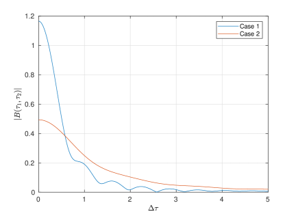
In our experiments, we will study two examples with the parameter settings listed below in Table 1. As one can observe from Figure 2, under the two parameter settings both decay to zero for large time difference, which guarantees the convergence of the Dyson series as well as the infinite series in the inchworm integro-differential equation (18).
In Case 2, the decay of is slower than Case 1, leading to a slower convergence of the Dyson series and the inchworm series. It can then be expected that larger needs to be included in the simulation of Case 2.
Table 1. Parameter settings for spin-boson model.
Parameters
Case 1
Case 2
Kondo parameter,
0.4
0.1
Inverse temperature,
5
0.2
Primary frequency,
2.5
1
Maximum frequency,
Energy difference,
1
1
Frequency of spin flipping,
1
1
Number of modes,
400
400
Figure 2. Two-point correlation functions under different parameter settings
4.1. Numerical experiments for computational complexity
In this section, we compare the wall clock time on evaluating given and using direct summation and Algorithms 1 and 2 based on the inclusion-exclusion principle. The experiments are carried out using MATLAB on Intel Xeon CPU X5650 and the results for the time consumed may vary for different hardware, programming languages and implementation details. Since the operation counts do not depend on the value of , we will only use the parameters for Case 1 in our test throughout this section.
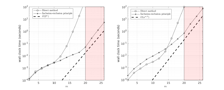
Figure 3. Wall clock time (seconds) on evaluating a given (left) and (right) using direct method and inclusion-exclusion principle in logarithm scale
The computational time for a various choice of is plotted in Figure 3. In the left panel, we compare direct method with Algorithm 1 for computing a given bath influence functional. As predicted, the efficiencies of the two algorithms are comparable for small order . Starting from , however, due to the double factorial growth in complexity, the time cost for the direct method becomes obviously larger than the inclusion-exclusion principle whose growth rate is only exponential as according to our discussion at the end of Section 2. The right panel of Figure 3 compares Algorithm 2 with the direct summation over the linked diagrams to compute a rounded box. Algorithm 2 outperforms the direct method when . The dotted line represents our estimation of the growth rate . We can observe that the curve of the inclusion-exclusion principle gradually becomes parallel to the dotted line, as indicates that our estimation of the computational complexity is sharp.
We would also like to discuss the memory cost of the algorithms. The direct method is out of memory for our machine once entering the red region (i.e., ) and thus the results are not presented. In our simulation, to implement the direct method efficiently, we first generate all the linked diagrams and store their configurations in the memory, so that the computational time presented in Figure 3 can be minimized. To store the diagrams, we use a matrix of size to record the indices of the time sequence in all linked diagrams. Here represents the number of diagrams, and denotes the length of the rounded box. For example, all the diagrams included in (see (21)) are stored in the following matrix
where each row of the matrix describes the pairing of time points (arcs) in one diagram on the right-hand side of (21). However, the size of this matrix grows quickly as increases due to the double factorial growth of the number of diagrams. For example, when the length of a rounded box reaches , the size of matrix turns out to be . Even if we use the uint8 data type in MATLAB (the smallest unsigned integer type that takes only one byte) to store the matrix, the total memory cost is around 89G, which is beyond the capacity of most machines. A workaround is to further compress the matrix using more compact storage patterns, or generate the diagrams during the summation. Both approaches will cause additional operations so that the computation may be further slowed down.
As a comparison, the major memory cost for inclusion-exclusion principle concentrates in the temporary storage of complex-valued and appearing in Theorem 1, which grows only as an exponential and the memory requirement is at most G (only 0.1344G for ). Here refers to the number of bytes for a double-precision complex number, and refers to the total number of entries in and . As a result, a longer diagram can be computed using the algorithm based on the inclusion-exclusion principle.
Such a memory issue for the direct method also exists when computing since the number of diagrams given by a bath influence functional is even larger than that in a rounded box of the same size.
4.2. Numerical simulations for open quantum systems
We now implement several numerical simulations on the observable using bare dQMC and inchworm Monte Carlo method respectively, in which inclusion-exclusion principle will be used to evaluate large rectangular and rounded boxes. We would like to check if and how frequently we will encounter the scenarios when the order has to be chosen very large during the simulations to show the necessity of exploiting the inclusion-exclusion principle.
4.2.1. Numerical methods
We first introduce the numerical methods for our simulations. In particular, we will discuss the details of the implementation of bare dQMC. For the more complicated inchworm equation, we only provide our Monte Carlo sampling method, which is novel in this work. One may refer to [10, 11] for the general framework of the full implementation.
In the Dyson series (3), should be chosen as even due to the Wick’s theorem for the bath influence functional. Moreover, the term in the Dyson series does not contain any time points and thus no Monte Carlo sampling is needed when applying bare dQMC. Therefore, we may take out this term and rewrite (3) as
To approximate the infinite series in the above formula using Monte Carlo integration, we need sample
•
a positive even number ;
•
a sequence of times: .
Once is chosen, the time sequence can be generated by drawing a sample from the uniform distribution and then sorting the sequence. In our previous works [10, 11], instead of sampling the even number , we simply truncated the series (3) at and use the same number of samples for each . In the current paper, we would propose a heuristic approach to take samples of . Ideally, the probability of should be proportional to the absolute value of the integral in (3). Since such a function is not available, we make the following approximations:
•
Ignore the term representing the system part;
•
Use the uniform distribution of to represent the value of in all cases.
Thus the distribution of becomes
(52)
where and is given such that the normalization holds. Here we set to be the maximum value of in order to prevent from being too large, which may cause unnecessary huge computational cost in the evaluation of the bath influence functional. Thereafter, the bare dQMC approximates the observable as
(53)
where is the number of samples, and the quantities with superscript denote the th sample.
In order to study the evolution of the observable in the time interval , we will need to compute all for given the time step (the initial value is according to the definition (2)). Therefore, we need to first generate for all , which requires the calculation of long including up to time points. This can be time-consuming when the time step is small, and it is also unnecessary for short time simulations where a large is unlikely to be sampled. To improve the efficiency of simulations, we consider a more accessible distribution to approximate . In (52), we insert the definition of the bath influence functional and reach to
where the constant is some average of the two-point correlation. Inspired by this formulation, we set to be a constant and choose the probability mass function to be , where is chosen such that the normalization holds. Thus each sample can be drawn based on the Poisson distribution. More precisely, we sample according to
(54)
Note that the “” is needed on the left-hand side above since a standard Poisson distribution samples nonnegative integers from 0 while begins with 1.
It remains only to set a suitable value for . Here we simply select such that the probability mass function of is close to (52) for .
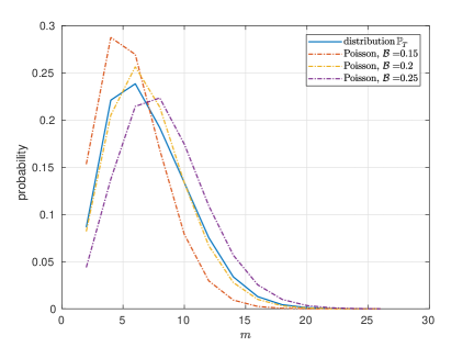
For example in Figure 4, one can compare the three probability mass functions of Poisson distributions with different for the numerical example Case 1 to see that the yellow dashed-dotted line gives a satisfactory approximation to . Poisson distributions with some other are plotted as references, which are comparatively far away from the target blue line. Therefore, we set for the Poisson distribution in Case 1.
Figure 4. Comparison between the distribution (52) and Poisson distributions with changing for parameter setting Case 1 with and .
To end this section, we provide a brief discussion on the key procedures of the sampling method in the implementation of the inchworm Monte Carlo method. In (18), the partial derivative on the left-hand side is discretized by a certain time integrator such as Heun’s method. As for the right-hand side, similar to the bare dQMC, we need to approximate the infinite series by sampling an even number and the time sequence at every time step. The time sequence is again sampled according to the uniform distribution , and the probability mass function of is analogous to (52):
(55)
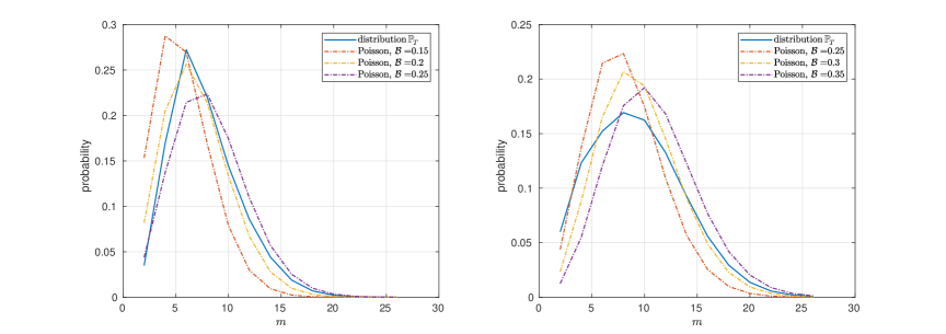
where . To avoid the expensive computations of the long rounded boxes , we also sample each applying the Poisson distribution (54) in practice, where the choice of is subject to a satisfactory approximation to the distribution (55), which is set to be and for Case 1 and Case 2, respectively. We refer the readers to Figure 5 for a comparison between the Poisson distribution and the distribution (55) for .
Figure 5. Comparison between the distribution (55) and Poisson distributions with changing for parameter setting Case 1 (left) and Case 2 (right) with and .
4.2.2. Numerical results
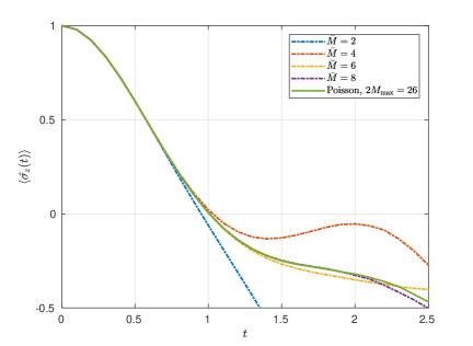
With the numerical methods introduced, we are now ready to present the results of our simulations on the time evolution of the observable . We are particularly interested in the convergence of computed by both bare dQMC and inchworm method w.r.t. the order . Specifically, we first perform the simulation with the series in (17) or (18) truncated at , and plot the real part of up to . Note that due to the numerical error, the computed may contain a nonzero imaginary part. We hope to observe the convergence of these results to the numerical solution using our approach introduced in Section 4.2.1, which justifies our numerical method. In our simulation, the Poisson distribution is truncated at , so that the maximum value of is .
Figure 6. Evolution of for parameter setting Case 1 by bare dQMC
Table 2. Large sampled by Poisson distribution in the simulation for Case 1 by bare dQMC
20
22
24
26
195123
44427
9197
1820
Figure 6 plots the numerical results for parameter setting Case 1 using bare dQMC. We set the time step to be and compute for each . For the result with sampled by Poisson distribution, each is calculated based on Monte Carlo samples. As for the results with fixed truncation , we evaluate each -dimensional integral in (3) using Monte Carlo samples. One can observe that the curve of observable tends to converge as grows. However, significant difference can still be observed between the results for and , indicating that larger needs to be taken into account to get reliable results, and thus considering also as a random variable turns out to be an efficient way to find suitable number of samples. With this approach, larger will be encountered in the simulation, and we have listed in Table 2 the number of large (within the red region of Figure 3) sampled by the Poisson distribution, which also represents the number of -point bath influence functionals evaluated in the entire simulation. For example, we need to compute 1820 independent for Monte Carlo integration using inclusion-exclusion principle. The evaluation of such high-order bath influence functionals is hardly feasible using the direct method.
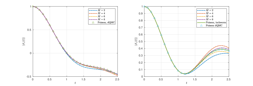
Figure 7. Evolution of for parameter setting Case 1 (left) and Case 2 (right) by inchworm Monte Carlo method
Table 3. Large sampled by Poisson distribution in the simulation for Case 2 by inchworm Monte Carlo method
20
22
24
26
17710
5336
1492
395
As for the simulations by inchworm Monte Carlo method, we refer to Figure 7 for the numerical results with both parameter settings Case 1 and Case 2. The time step is again set as , while the number of samples is chosen as a relatively smaller ( denotes the total number of samples used in the simulation by Poisson distribution, and the number of samples used for each -dimensional integral in the simulations with fixed truncation) since the numerical error of inchworm method is generally smaller than that of classic Dyson series [10]. For Case 1, the curve with fixed becomes almost identical to thanks to the rapid convergence of inchworm method. The result by bare dQMC using Poisson distribution (same as the solid line in Figure 6) is given as a reference. This indicates that inchworm Monte Carlo method can provide a satisfactory approximation to the exact solution with a small truncation and hence outperform bare dQMC for this set of parameters. As no larger is needed, there is no need to apply the inclusion-exclusion principle in this case. However in Case 2, the inchworm Monte Carlo method also suffers from slow convergence due to the slow decay of the two-point correlation function (see Figure 2). The right panel of Figure 7 shows that the discrepancy between and is still noticeable. With the adaptive choice of , we are able to obtain results in good agreement with the reference results provide by bare dQMC with samples for each . Again, we list in Table 3 the number of samples involving large in this experiment to show that inclusion-exclusion principle is indispensable to the calculation of long rounded boxes that direct method cannot deal with.
5. Conclusion
We have proposed fast algorithms based on inclusion-exclusion principle to sum diagrams appearing in the bare dQMC and inchworm Monte Carlo method. For bare dQMC, we have developed a formula to efficiently evaluate the bosonic bath influence functional at the cost of . Note that in the fermionic case, the bath influence functional becomes a determinant [27, 42], while in the bosonic case, the computational cost is higher, but it turns out that the computational complexity is lower than the Ryser’s algorithm for matrix permanents.
For the inchworm method, our algorithm calculating the sum over linked diagrams can be considered as an extension to the work [8] which deals with the fermionic quantum impurity models. By a detailed complexity analysis, we have proved that the new algorithm reduces the computational cost from the original double factorial to exponential. More precisely, we estimate the computational complexity as where , which has been also verified by our numerical experiments. Moreover, numerical simulations for the spin-boson model have been implemented to show the advantages of our approaches.
Appendix A Formulas of functionals
A.1. Definition of
The system related functional in the Dyson series (3) is defined by
where
A.2. Definition of
The functional in the integro-differential equation (18) is given by
where the full propagator is defined by
with the propagator associated with the bath
The full propagator satisfies
•
Jump condition:
•
Boundary condition: .
Appendix B MATLAB code for computing the hafnian
Below we provide our MATLAB code to compute the hafnian of a symmetric matrix . The input matrix needs to be a symmetric square matrix with all diagonal entries being zero.
[1]
Andrey E. Antipov, Qiaoyuan Dong, Joseph Kleinhenz, Guy Cohen, and Emanuel
Gull.
Currents and green’s functions of impurities out of equilibrium:
Results from inchworm quantum monte carlo.
Phys. Rev. B, 95:085144, Feb 2017.
[2]
A. Barvinok.
Polynomial time algorithms to approximate permanents and mixed
discriminants within a simply exponential factor.
In Random Structures & Algorithms, pages 29–61, 1999.
[3]
M. H. Beck, A. jackle, G. A. Worth, and H. D. Meyer.
The multiconfiguration time-dependent hartree (mctdh) method: a
highly efficient algorithm for propagating wavepackets.
Phys. Rep., 324:1–105, 2000.
[4]
A. BJörklund.
Counting perfect matchings as fast as Ryser.
In Y. Rabani, editor, Proceedings of the 2012 Annual ACM-SIAM
Symposium on Discrete Algorithms, pages 914–921, 2012.
[5]
A. Björklund, B. Gupt, and N. Quesada.
A faster hafnian formula for complex matrices and its benchmarking on
a supercomputer.
ACM J. Exp. Algorithmics, 24, 2019.
[6]
A. Björklund and T. Husfeldt.
Exact algorithms for exact satisfiability and number of perfect
matchings.
Algorithmica, 52:226–249, 2008.
[7]
A. BJörklund, T. Husfeldt, and M. Koivisto.
Set partitioning via inclusion-exclusion.
SIAM J. Comput., 39(2):546–563, 2009.
[8]
Aviel Boag, Emanuel Gull, and Guy Cohen.
Inclusion-exclusion principle for many-body diagrammatics.
Phys. Rev. B, 98:115152, 2018.
[9]
H. Breuer and F. Petruccione.
The Theory of Open Quantum Systems.
Oxford University Press, 2007.
[10]
Z. Cai, J. Lu, and S. Yang.
Numerical analysis for inchworm monte carlo method: Sign problem and
error growth.
arXiv:2006.07654.
[11]
Z. Cai, J. Lu, and S. Yang.
Inchworm monte carlo method for open quantum systems.
Communications on Pure and Applied Mathematics,
73(11):2430–2472, 2020.
[12]
H.-T. Chen, G. Cohen, and D. R. Reichman.
Inchworm Monte Carlo for exact non-adiabatic dynamics. I.
Theory and algorithms.
J. Chem. Phys., 146:054105, 2017.
[13]
H.-T. Chen, G. Cohen, and D. R. Reichman.
Inchworm Monte Carlo for exact non-adiabatic dynamics. II.
Benchmarks and comparison with established methods.
J. Chem. Phys., 146:054106, 2017.
[14]
G. Cohen, E. Gull, D. R. Reichman, and A. J. Millis.
Taming the dynamical sign problem in real-time evolution of quantum
many-body problems.
Phys. Rev. Lett., 115(26):266802, 2015.
[15]
M. Cygan and M. Pilipczuk.
Faster exponential-time algorithms in graphs of bounded average
degree.
Information and Computation, 243:75–85, 2015.
[16]
E. B. Davies.
Markovian master equations.
Commun. Math. Phys., 39(2):91–110, 1974.
[17]
E. B. Davies.
Markovian master equations. II.
Math. Ann., 219(2):147–158, 1976.
[18]
Q. Dong, I. Krivenko, J. Kleinhenz, A. E. Antipov, G. Cohen, and E. Gull.
Quantum Monte Carlo solution of the dynamical mean field
equations in real time.
Phys. Rev. B, 96:155126, 2017.
[19]
C. Duan, Z. Tang, J. Cao, and J. Wu.
Zero-temperature localization in a sub-ohmic spin-boson model
investigated by an extended hierarchy equation of motion.
Phys. Rev. B, 95(21):214308, 2017.
[20]
Emanuel Gull, Andrew J. Millis, Alexander I. Lichtenstein, Alexey N. Rubtsov,
Matthias Troyer, and Philipp Werner.
Continuous-time Monte Carlo methods for quantum impurity models.
Rev. Mod. Phys., 83:349–404, 2011.
[21]
R. Kan.
From moments of sum to moments of product.
Journal of Multivariate Analysis, 99(3):542–554, 2008.
[22]
L. V. Keldysh.
Diagram technique for nonequilibrium processes.
Sov. Phys. JETP, 20(4):1018–1026, 1965.
[23]
D. Mac Kernan, G. Ciccotti, and R. Kapral.
Surface-hopping dynamics of a spin-boson system.
J. Chem. Phys., 116(6):2346–2353, 2002.
[24]
M. Koivisto.
Partitioning into sets of bounded cardinality.
In Parameterized and Exact Computation, pages 258–263.
Springer Berlin Heidelberg, 2009.
[25]
N. Makri.
Numerical path integral techniques for long time dynamics of quantum
dissipative systems.
J. Math. Phys., 36(5):2430–2457, 1995.
[26]
N. Makri, E. Sim, D. E. Makarov, and M. Topaler.
Long-time quantum simulation of the primary charge separation in
bacterial photosynthesis.
Proc. Natl. Acad. Sci., 93(9):3926–3931, 1996.
[27]
L. Mühlbacher and E. Rabani.
Real-time path integral approach to nonequilibrium many-body quantum
systems.
Phys. Rev. Lett., 100(17):176403, 2008.
[28]
L. Mühlbacher and E. Rabani.
Diagrammatic Monte Carlo simulation of nonequilibrium systems.
Phys. Rev. B, 79(3):035320, 2009.
[29]
J. Nederlof.
Fast polynomial-space algorithms using möbius inversion:
Improving on steiner tree and related problems.
In Automata, Languages and Programming, pages 713–725.
Springer Berlin Heidelberg, 2009.
[30]
J.W. Negele and H. Orland.
Quantum Many-particle Systems.
Advanced Book Classics. Basic Books, 1988.
[31]
M. A. Nielsen and I. L. Chuang.
Quantum Computation and Quantum Information: 10th Anniversary
Edition.
Cambridge University Press, 2010.
[32]
M. Ridley, V. N. Singh, E. Gull, and G. Cohen.
Numerically exact full counting statistics of the nonequilibrium
Anderson impurity model.
Phys. Rev. B, 97(11):115109, 2018.
[33]
Riccardo Rossi.
Determinant diagrammatic monte carlo algorithm in the thermodynamic
limit.
Phys. Rev. Lett., 119:045701, 2017.
[34]
HERBERT JOHN RYSER.
Combinatorial Mathematics, volume 14.
Mathematical Association of America, 1 edition, 1963.
[35]
M. Schiró.
Real-time dynamics in quantum impurity models with diagrammatic
Monte Carlo.
Phys. Rev. B, 81(8):085126, 2010.
[36]
Marco Schiró and Michele Fabrizio.
Real-time diagrammatic monte carlo for nonequilibrium quantum
transport.
Phys. Rev. B, 79:153302, 2009.
[37]
P. R. Stein.
On a class of linked diagrams, II. Asymptotics.
Discrete Math., 21:309–318, 1978.
[38]
Y. Tanimura.
Nonperturbative expansion method for a quantum system coupled to a
harmonic-oscillator bath.
Phys Rev A., 41(0):6676–6687., 1990.
[39]
Y. Tanimura and R. Kubo.
Time evolution of a quantum system in contact with a nearly
gaussian-markoffian noise bath.
J. Phys. Soc. Jpn., 58(1):101–114, 1989.
[40]
G. Thomas and R. Finney.
Calculus and Analytic Geometry, 7th Edition.
Addison-Wesley Publishing Company, 1988.
[41]
H. Wang.
Basis set approach to the quantum dissipative dynamics: Application
of the multiconfiguration time-dependent Hartree method to the spin-boson
problem.
J. Chem. Phys., 113(22):9948–9956, 2000.
[42]
Philipp Werner, Armin Comanac, Luca de’ Medici, Matthias Troyer, and Andrew J.
Millis.
Continuous-time solver for quantum impurity models.
Phys. Rev. Lett., 97:076405, 2006.