Data-driven computation methods for quasi-stationary distribution and sensitivity analysis

Abstract.

This paper studies computational methods for quasi-stationary distributions (QSDs). We first proposed a data-driven solver that solves Fokker-Planck equations for QSDs. Similar as the case of Fokker-Planck equations for invariant probability measures, we set up an optimization problem that minimizes the distance from a low-accuracy reference solution, under the constraint of satisfying the linear relation given by the discretized Fokker-Planck operator. Then we use coupling method to study the sensitivity of a QSD against either the change of boundary condition or the diffusion coefficient. The 1-Wasserstein distance between a QSD and the corresponding invariant probability measure can be quantitatively estimated. Some numerical results about both computation of QSDs and their sensitivity analysis are provided.

1. Introduction

Many models in various applications are described by Markov chains with absorbing states. For example, any models with mass-action kinetics, such as ecological models, epidemic models, and chemical reaction models, are subject to the population-level randomness called the demographic stochasticity, which leads to extinction in finite time. There are also many dynamical systems that have interesting short term dynamics but trivial long term dynamics, such as dynamical systems with transient chaos [15]. A common way of capturing asymptotical properties of these transient dynamics is the quasi-stationary distribution (QSD), which is the conditional limiting distribution conditioning on not hitting the absorbing set yet. However, most QSDs do not have a closed form. So numerical solutions are necessary in various applications.

Computational methods for QSDs are not very well developed. Although the relation between QSD and the Fokker-Planck equation is well known, it is not easy to use classical PDE solver to solve QSDs because of the following two reasons. First a QSD is the eigenfunction of the Fokker-Planck operator whose eigenvalue is unknown. The cost of solving eigenfunction of a discretized Fokker-Planck operator is considerably high. Secondly the boundary condition of the Fokker-Planck equation is unknown. We usually have a mixture of unbounded domain and unknown boundary value at the absorbing set. As a result, Monte Carlo simulations are more commonly used. However the efficiency of the Monte Carlo simulation is known to be low. To get the probability density function, one needs to deal with undesired noise associated to the Monte Carlo simulation. Methods like the kernel density estimator can smooth the solution but also introduce undesired diffusions to the solution, especially when a QSD is highly concentrated at the vicinity of some low-dimensional sets.

The first goal of this paper is to extend the data-driven Fokker-Planck solver developed by the first author to the case of QSDs [7]. Similar to [7], we need a reference solution $\mathbf{v}$ generated by the Monte Carlo simulation. Then we discretize the Fokker-Planck operator in a numerical domain $D$ without the boundary condition. Because of the lack of boundary conditions, the discretization only gives an underdetermined linear system, denoted by $\mathbf{Au}=0$. Then we minimize $\|\mathbf{v}-\mathbf{u}\|$ in the null space of $\mathbf{A}$. As shown in [8], this optimization problem projects the error terms of $\mathbf{v}$ to a low dimensional linear subspace, which significantly reduces its norm. Our numerical simulations show that this data-driven Fokker-Planck solver can tolerate very high level of spatially uncorrelated error, so the accuracy of $\mathbf{v}$ does not have to be high. The main difference between QSD solver and the Fokker-Planck solver is that we need a killing rate to find the QSD, which is obtained by a Monte Carlo simulation. We find that the QSD is not very sensitive against small error in the estimation of the killing rate.

The second goal of this paper is to study the sensitivity of QSDs. Some modifications of either the boundary condition or the model parameters can prevent the Markov process from hitting the absorbing state in finite time. So the modified process would admit an invariant probability measure instead of a QSD. It is important to understand the difference between the QSD of a Markov process and the invariant probability measure of its modification. For example, many ecological models do not consider demographic noise because the population size is large and the QSD is much harder to study. But would the demographic noise completely change the asymptotical dynamics? More generally, a QSD captures the transient dynamics of a stochastic differential equation. If we separate a domain from the global dynamics by imposing reflecting boundary condition, how would the local dynamics be different from the corresponding transient dynamics? All these require some sensitivity analysis with quantitative bounds.

The way of sensitivity analysis is similar to [8]. We need both finite time error and the rate of contraction of the transition kernel of the Markov process. The finite time error is given by both the killing rate and the change of model parameters (if any). Both cases can be estimated easily. The rate of contraction is estimated by the data-driven method proposed in [17]. We design a suitable coupling scheme for the modified Markov process that admits an invariant probability measure. Because of the coupling inequality, the exponential tail of the coupling time can be used to estimate the rate of contraction. The sensitivity analysis is demonstrated by several numerical examples. We can find that the invariant probability measure of the modified process is a better approximation of the QSD if (i) the speed of contraction is faster and (ii) the killing rate is lower.

The organization of this paper is as follows. A short preliminary about QSD, Fokker-Planck equation, simulation method, and coupling method is provided in Section 2. Section 3 introduces the data-driven QSD solver. The sensitivity analysis of QSD is given in Section 4. Section 5 is about numerical examples.

2. Preliminary

In this section, we provide some preliminaries to this paper, which are about the quasi-stationary distribution (QSD), the Fokker-Planck equation, the coupling method, and numerical simulations of the QSD.

2.1. Quasi-stationary distribution

We first give definition of the QSD and the exponential killing rate $\lambda$ of a Markov process with an absorbing state. Let $X=(X_{t}:t\geq 0)$ be a continuous-time Markov process taking values in a measurable space $(\mathcal{X},\mathcal{B}(\mathcal{X}))$. Let $P^{t}(x,\cdot)$ be the transition kernel of $X$ such that $P^{t}(x,A)=\mathbb{P}[X_{t}\in A\,|\,X_{0}=x]$ for all $A\in\mathcal{B}$. Now assume that there exists an absorbing set $\partial\mathcal{X}\subset\mathcal{X}$. The complement $\mathcal{X}^{a}:=\mathcal{X}\backslash\partial\mathcal{X}$ is the set of allowed states.

The process $X_{t}$ is killed when it hits the absorbing set, implying that $X_{t}\in\partial\mathcal{X}$ for all $t>\tau$, where $\tau=\inf\{t>0:X_{t}\in\partial\mathcal{X}\}$ is the hitting time of set $\partial\mathcal{X}$. Throughout this paper, we assume that the process is almost surely killed in finite time, i.e. $\mathbb{P}[\tau<\infty]=1$.

For the sake of simplicity let $\mathbb{P}_{x}$ (resp. $\mathbb{P}_{\mu}$) be the probability conditioning on the initial condition $x\in\mathcal{X}$ (resp. the initial distribution $\mu$).

Definition 2.1.

A probability measure $\mu$ on $\mathcal{X}^{a}$ is called a quasi-stationary distribution(QSD) for the Markov process $X_{t}$ with an absorbing set $\partial\mathcal{X}$, if for every measurable set $C\subset\mathcal{X}^{a}$

(2.1) $$\mathbb{P}_{\mu}[X_{t}\in C|\tau>t]=\mu(C),\ t\geq 0,$$

or equivalently, if there is a probability measure $\mu$ exists such that

(2.2) $$\lim_{t\rightarrow\infty}\mathbb{P}_{\mu}[X_{t}\in C|\tau>t]=\mu(C).$$

in which case we also say that $\mu$ is a quasi-limiting distribution.

Remark 2.1.

When $\mu$ satisfies (2.2), it is called a quasi-limiting distribution, or a Yaglom limit [6] .

In the analysis of QSD, we are particularly interested in a parameter $\lambda$, called the killing rate of the Markov process. If the distribution of the killing time $\mathbb{P}_{x}(\tau>t)$ has an exponential tail, then $\lambda$ is the rate of this exponential tail. The following theorem shows that the killing time is exponentially distributed when the process starts from a QSD[5].

Theorem 2.1.

Let $\mu$ be a QSD and when starting from $\mu$, the killing time $T$ is exponentially distributed, that is,

$$\exists\ \lambda=\lambda(\mu)\ \text{such that}\ \mathbb{P}_{\mu}[\tau>t]=e^{-\lambda t},\ \forall t\geq 0,$$

where $\lambda$ is called the killing rate of $X$.

Throughout this paper, we assume that $X$ admits a QSD denoted by $\mu$ with a strictly positive killing rate $\lambda$.

2.2. Fokker-Planck equation

Consider a stochastic differential equation

(2.3) $$\text{d}X_{t}=f(X_{t})\text{d}t+\sigma(X_{t})\text{d}W_{t},$$

where $X_{t}\in\mathbb{R}^{d}$ and $X_{t}$ is killed when it hits the absorbing set $\partial\mathcal{X}\subset\mathbb{R}^{n}$; $f:\mathbb{R}^{d}\rightarrow\mathbb{R}^{d}$ is a continuous vector field; $\sigma$ is an $d\times d$ matrix-valued function; and $\text{d}W_{t}$ is the white noise in $\mathbb{R}^{d}$. The following well known theorem shows the existence and the uniqueness of the solution of equation (2.3).

Theorem 2.2.

Assume that there are two positive constants $C_{1}$ and $C_{2}$ such that the two functions $f$ and $\sigma$ in (2.3) satisfy
(1) (Lipschitz condition) for all $x,y\in\mathbb{R}^{d}$ and $t$

$$|f(x)-f(y)|^{2}+|\sigma(x)-\sigma(y)|^{2}\leq C_{1}|x-y|^{2};$$

(2) (Linear growth condition) for all $x,y\in\mathbb{R}^{d}$ and $t$

$$|f(x)|^{2}+|\sigma(x)|^{2}\leq C_{2}(1+|x|^{2}).$$

Then there exists a unique solution $X(t)$ to equation (2.3).

There are quite a few recent results about the existence and convergence of QSD. Since the theme of this paper is numerical computations, in this paper we directly assume that $X_{t}$ admits a unique QSD $\mu$ on set $\mathcal{X}^{a}$ that is also the quasi-limit distribution. The detailed conditions are referred in [18, 13, 20, 9, 21].

Let $u$ be the probability density function of $\mu$. We refer [2] for the fact that $u$ satisfies

(2.4) $$-\lambda u=\mathcal{L}u=-\sum^{d}_{i=1}(f_{i}u)_{x_{i}}+\frac{1}{2}\sum^{d}_{i,j=1}(D_{ij}u)_{x_{i}x_{j}},$$

where $D=\sigma^{T}\sigma$, and $\lambda$ is the killing rate.

2.3. Simulation algorithm of QSD

It remains to review the simulation algorithm for QSDs. In order to compute the QSD, one needs to numerically simulate a long trajectory of $X$. Once $X_{t}$ hits the absorbing state, a new initial value is sampled from the empirical QSD. The re-sampling step can be done in two different ways. We can either use many independent trajectories that form an empirical distribution [3] or re-sample from the history of a long trajectory [19]. In this paper we use the latter approach.

Let $\hat{X}^{\delta}=\{\hat{X}^{\delta}_{n},\ n\in\mathbb{Z}_{+}\}$ be a long numerical trajectory of the time-$\delta$ sample chain of $X_{t}$, where $\hat{X}^{\delta}_{n}$ is an numerical approximation of $X_{n\delta}$, then the Euler-Maruyama numerical scheme is given by

(2.5) $$\hat{X}^{\delta}_{n+1}=\hat{X}^{\delta}_{n}+f(\hat{X}^{\delta}_{n})\delta+\sigma(\hat{X}^{\delta}_{n})(W_{(n+1)\delta}-W_{n\delta}),$$

where $\hat{X}^{\delta}_{n}=X_{0}$, $W_{(n+1)\delta}-W_{n\delta}\sim\mathcal{N}(0,\delta\mathrm{Id}_{d}),\ n\in\mathbb{Z}_{+}$ is a $d$-dimensional normal random variable.

Another widely used numerical scheme is called the Milstein scheme, which reads

$$\hat{X}^{\delta}_{t}=\hat{X}^{\delta}_{n}+f(\hat{X}^{\delta}_{n})(t-n\delta)+\sigma(\hat{X}^{\delta}_{n})(W_{t}-W_{n\delta})+\sigma(\hat{X}^{\delta}_{n})IL,$$

where $I$ is a $d\times d$ matrix with its $(i,j)$-th component being the double It$\hat{o}$ integral

$$I_{i,j}=\int^{t}_{n\delta}\int^{s}_{n\delta}dW^{i}(s_{1})dW^{j}(s_{2}),$$

and $L\in\mathbb{R}^{d}$ is a vector of left operators with $i$-th component

$$u\mathcal{L}_{i}=\sum^{d}_{i=1}\sigma_{i,j}(\hat{X}^{\delta}_{n})\frac{\partial u}{\partial x_{i}}.$$

Remark 2.2.

Under suitable assumptions of Lipschitz continuity and linear growth conditions for $f$ and $\sigma$, the Euler-Maruyama approximation provides a convergence rate of order 1/2, while the Milstein scheme is an order 1 strong approximation[14].

For simplicity, we introduce the algorithm for $n=2$, specifically, we solve $u$ in equation (2.4) numerically on a 2D domain $D=[a_{0},b_{0}]\times[a_{1},b_{1}]$. Firstly, we construct an $N\times M$ grid on $D$ with grid size $h=\frac{b_{0}-a_{0}}{N}=\frac{b_{1}-a_{1}}{M}$. Each small box in the mesh is denoted by $O_{i,j}=[a_{0}+(i-1)h,a_{0}+ih]\times[a_{1}+(j-1)h,a_{1}+jh]$. Let $\mathbf{u}=\{u_{i,j}\}^{i=N,j=M}_{i=1,j=1}$ be the numerical solution on $D$ that we are interested in, then $\mathbf{u}$ can be considered as a vector in $\mathbb{R}^{N\times M}$. Each element $u_{i,j}$ approximates the density function $u$ at the center of each $O_{i,j}$, with coordinate $(ih+a_{0}-h/2,jh+a_{1}-h/2)$. Generally speaking, we count the number of $\hat{X}^{\delta}$ falling into each box and set the normalized value as the approximate probability density at $O_{i,j}$. As we are interested in the QSD, the main difference from the general Monte Carlo is that the Markov process will be regenerated as the way of its empirical distribution uniformly once it is killed. The details of simulation is shown in Algorithm 1 as following.

Algorithm 1 Monte Carlo for QSD

0:  Equation (2.5) and the grid

0:  A Monte Carlo approximation $\mathbf{u}=\{u_{i,j}\}$. Sample size $N_{s}$.

  Pick any initial value $X_{0}\notin\partial\mathcal{X}$ in $D$

  for $n=1\ \text{to}\ N_{s}$ do

     Use $\hat{X}^{\delta}_{n}$ and equation (2.5) to compute $\hat{X}^{\delta}_{n+1}$

     Record the coordinates of the small box $O_{i,j}$ where $\hat{X}^{\delta}_{n+1}$ stands, say $i^{*},j^{*}$

     if $\hat{X}^{\delta}_{n+1}\notin\partial\mathcal{X}$ then

        $u_{i^{*},j^{*}}\leftarrow u_{i^{*},j^{*}}+1$

     else

        $\hat{X}^{\delta}_{n+1}=\hat{X}^{\delta}_{\lfloor U*n\rfloor}$,  where $U$ is a uniformly distributed random variable

     end if

  end for

  Return $u_{i,j}/N_{s}h^{2}$ for all $i,j$ as the approximation solution.

Sometimes the Euler-Maruyama method underestimates the probability that $X$ moves to the absorbing set, especially when $X_{t}$ is close to $\partial\mathcal{X}$. This problem can be fixed by introducing the Brownian bridge correction. We refer to [4] for details. For a sample falling into a small box which are closed to $\partial\mathcal{X}$, the probability of them falling into the trap $\partial\mathcal{X}$ is relatively high. In fact, this probability is exponentially distributed and the rate is related to the distance from $\partial\mathcal{X}$. Let $B^{T}_{B}=W_{t}-\frac{t}{T}W_{T}$ be the Brownian Bridge on the interval $[0,T]$. In the 1D case, the law of the infimum and the supremum of the Brownian Bridge can be computed as follows: for every $z\geq\max(x,y)$

(2.6) $$\mathbb{P}[\sup_{t\in[0,T]}(x+(y-x)\frac{t}{T}+\phi B^{T}_{B})\leq z]=1-\exp(-\frac{2}{T\phi^{2}}(z-x)(z-y)),$$

where $x=\hat{X}^{\delta}_{n}\in\mathcal{X}^{a},y=\hat{X}^{\delta}_{n+1}\in\mathcal{X}^{a}$, and $\phi=\sigma(\hat{X}^{\delta}_{n})$ is the strength coefficient of Brownian Bridge. This means that at each step $n$, if $\hat{X}^{\delta}_{n+1}\in\mathcal{X}^{a}$, one can compute, with the help of the above properties, a Bernoulli random variable $G$ with the parameter

$$p=\mathbb{P}[\exists t\in(n\delta,(n+1)\delta),\hat{X_{t}}\in\partial\mathcal{X}|x=\hat{X}^{\delta}_{n},y=\hat{X}^{\delta}_{n+1}]\ \ (\text{If}\ G=1,\text{the process is killed}).$$

2.4. Coupling Method

The coupling method is used for the sensitivity analysis of QSDs.

Definition 2.2.

(Coupling of probability measures) Let $\mu$ and $\nu$ be two probability measures on a probability space $(\Omega,\mathcal{F})$. A probability measure $\gamma$ on $(\Omega\times\Omega,\mathcal{F}\times\mathcal{F})$ is called a coupling of $\mu$ and $\nu$, if two marginals of $\gamma$ coincide with $\mu$ and $\nu$ respectively.

The definition of coupling can be extended to any two random variables that take value in the same state space. Now consider two Markov processes $X=(X_{t}:t\geq 0)$ and $Y=(Y_{t}:t\geq 0)$ with the same transition kernel $P$. A coupling of $X$ and $Y$ is a stochastic process $(\widetilde{X},\widetilde{Y})$ on the product state space $\mathcal{X}\times\mathcal{X}$ such that

(i) The marginal processes $\widetilde{X}$ and $\widetilde{Y}$ are Markov processes with the transition kernel $P$;

(ii) If $\widetilde{X_{s}}=\widetilde{Y_{s}}$, we have $\widetilde{X_{t}}=\widetilde{Y_{t}}$ for all $t>s$.

The first meeting time of $X_{t}$ and $Y_{t}$ is denoted as $\tau^{C}:=\inf_{t\geq 0}\{X_{t}=Y_{t}\}$, which is called the coupling time. The coupling $(\widetilde{X},\widetilde{Y})$ is said to be successful if the coupling time is almost surely finite, i.e. $\mathbb{P}[\tau^{C}<\infty]=1$.

In order to give an estimate of the sensitivity of the QSD, we need the following two metrics.

Definition 2.3.

(Wasserstein distance) Let $d$ be a metric on the state space $V$. For probability measures $\mu$ and $\nu$ on $V$, the Wasserstein distance between $\mu$ and $\nu$ for $d$ is given by

(2.7) $$\begin{split}d_{w}(\mu,\nu)&=\inf\{\mathbb{E}_{\gamma}[d(x,y)]:\ \gamma\ \text{is a coupling of }\mu\ and\ \nu.\}\\ &=\inf\{\int d(x,y)\gamma(dx,dy):\gamma\ \text{is a coupling of }\mu\ and\ \nu.\}\end{split}$$

In this paper, without further specification, we assume that the 1-Wasserstein distance is induced by $d(x,y)=\max\{1,\|x-y\|\}.$

Definition 2.4.

(Total variation distance) Let $\mu$ and $\nu$ be probability measures on $(\Omega,\mathcal{F})$. The total variation distance of $\mu$ and $\nu$ is

$$\|\mu-\nu\|_{TV}:=\sup_{C\in\mathcal{F}}|\mu(C)-\nu(C)|.$$

Lemma 2.3.

(Coupling inequality) For the coupling given above and the Wasserstein distance induced by the distance given in (2.7), we have

$$\mathbb{P}[\tau^{C}>t]=\mathbb{P}[X^{t}\neq Y^{t}]\geq d_{w}(P^{t}(x,\cdot),P^{t}(y,\cdot)).$$

Proof.

By the definition of Wasserstein distance,

$$\begin{split}d_{w}(P^{t}(x,\cdot),P^{t}(y,\cdot))&\leq\int d(x,y)\mathbb{P}[(\widetilde{X^{t}},\widetilde{Y^{t}})\in(dx,dy)]\\ &=\int_{x\neq y}d(x,y)\mathbb{P}[(\widetilde{X^{t}},\widetilde{Y^{t}})\in(dx,dy)]\\ &\leq\int_{x\neq y}\mathbb{P}[](\widetilde{X^{t}},\widetilde{Y^{t}})\in(dx,dy)]\\ &=\mathbb{P}[\widetilde{X^{t}}\neq\widetilde{Y^{t}}].\end{split}$$

∎

Consider a Markov coupling $(\widetilde{X},\widetilde{Y})$ where $\widetilde{X}_{t}$ and $\widetilde{Y}_{t}$ are two numerical trajectories of the stochastic differential equation described in (2.5). Theoretically, there are many ways to make stochastic differential equations couple. But since numerical computation always has errors, two numerical trajectories may miss each other when the true trajectories couple. Hence we need to apply a mixture of the following coupling methods in practice.

Independent coupling. Independent coupling means the noise term in the two marginal processes $X_{t}$ and $Y_{t}$ are independent when running the coupling process $(\widetilde{X},\widetilde{Y})$. That is

$$\begin{split}X^{\delta}_{n+1}&=f(X^{\delta}_{n})+(W^{(1)}_{(n+1)\delta}-W^{(1)}_{n\delta})\\ Y^{\delta}_{n+1}&=f(Y^{\delta}_{n})+(W^{(2)}_{(n+1)\delta}-W^{(2)}_{n\delta}),\end{split}$$

where $(W^{(1)}_{(n+1)\delta}-W^{(1)}_{n\delta})$ and $(W^{(2)}_{(n+1)\delta}-W^{(2)}_{n\delta})$ are independent random variables for each $n$.

Reflection coupling Two Wiener processes meet less often than the 1D case when the state space has higher dimensions. This fact makes the independent coupling less effective. The reflection coupling is introduced to avoid this case. Take the Euler-Maruyama scheme of the SDE

$$dX_{t}=f(X_{t})dt+\sigma dW_{t}$$

as an example, where $\sigma$ is a constant matrix. The Euler-Maruyama scheme of $X_{t}$ reads as

$$\hat{X}^{\delta}_{n+1}=\hat{X}^{\delta}_{n}+f(\hat{X}^{\delta}_{n})\delta+\sigma(W_{(n+1)\delta}-W_{n\delta}),$$

where $W$ is a standard Wiener process. The reflection coupling means that we run $\hat{X}^{\delta}_{n}$ as

$$\hat{X}^{\delta}_{n+1}=\hat{X}^{\delta}_{n}+f(\hat{X}^{\delta}_{n})\delta+\sigma(W_{(n+1)\delta}-W_{n\delta}),$$

while run $\hat{Y}^{\delta}_{n}$ as

$$\hat{Y}^{\delta}_{n+1}=\hat{Y}^{\delta}_{n}+f(\hat{Y}^{\delta}_{n})\delta+\sigma P(W_{(n+1)\delta}-W_{n\delta}),$$

where $P=I-2e_{n}e^{T}_{n}$ is a projection matrix with

$$e_{n}=\frac{\sigma^{-1}(\hat{X}^{\delta}_{n}-\hat{Y}^{\delta}_{n})}{\|\sigma^{-1}(\hat{X}^{\delta}_{n}-\hat{Y}^{\delta}_{n})\|}.$$

Nontechnically, reflecting coupling means that the noise term is reflected against the hyperplane that orthogonally passes the midpoint of the line segment connecting $\hat{X}^{\delta}_{n}$ and $\hat{Y}^{\delta}_{n}$. In particular, $e_{n}=-1$ when the state space is 1D.

Maximal coupling Above coupling schemes can bring $\hat{X}^{\delta}_{n}$ moves close to $\hat{Y}^{\delta}_{n}$ when running numerical simulations. However, a mechanism is required to make $\hat{X}^{\delta}_{n+1}=\hat{Y}^{\delta}_{n+1}$ with certain positive probability. That’s why the maximal coupling is involved. One can couple two trajectories whenever the probability distributions of their next step have enough overlap. Denote $p^{(x)}(x)$ and $p^{(y)}(x)$ as the probability density functions of $\hat{X}_{n+1}$ and $\hat{Y}_{n+1}$ respectively. The implementation of the maximal coupling is described in the following algorithm.

Algorithm 2 Maximal coupling

0:  $\hat{X}^{\delta}_{n}$ and $\hat{Y}^{\delta}_{n}$

0:  $\hat{X}^{\delta}_{n+1}$ and $\hat{Y}^{\delta}_{n+1}$, and $\tau^{C}$ if coupled

  Compute probability density functions $p^{(x)}(z)$ and $p^{(y)}(z)$

  Sample $\hat{X}^{\delta}_{n+1}$ and calculate $r=Up^{(x)}(\hat{X}^{\delta}_{n+1})$, where $U$ is uniformly distributed on [0,1]

  if $r<p^{(y)}(\hat{X}^{\delta}_{n+1})$ then

     $\hat{Y}^{\delta}_{n+1}=\hat{X}^{\delta}_{n+1},\tau^{C}=(n+1)\delta$

  else

     Sample $\hat{Y}^{\delta}_{n+1}$ and calculate $r^{\prime}=Vp^{(y)}(\hat{Y}^{\delta}_{n+1})$, where $V$ is uniformly distributed on [0,1]

     while $r^{\prime}<p^{(x)}(\hat{Y}^{\delta}_{n+1})$ do

        Resample $\hat{Y}^{\delta}_{n+1}$ and $V$. Recalculate $r^{\prime}=Vp^{(y)}(\hat{Y}^{\delta}_{n+1})$

     end while

     $\tau^{C}$ is still undetermined

  end if

For discrete-time numerical schemes of SDEs, we use reflection coupling when $\hat{X}^{\delta}_{n}$ and $\hat{Y}^{\delta}_{n}$ are far away from each other, and maximal coupling when they are sufficiently close. The threshold of changing coupling method is $2\sqrt{\delta}\|\sigma\|$ in our simulation, that is, the maximal coupling is applied when the distance between $\hat{X}^{\delta}_{n}$ and $\hat{Y}^{\delta}_{n}$ is smaller than the threshold.

3. Data-driven solver for QSD

Recall that the probability density function $u$ of QSD solves the Fokker-Planck equation $-\lambda u=\mathcal{L}u$. The QSD solver consists of three components: an estimator of the killing rate $\lambda$, a Monte Carlo simulator of QSD that produces a reference solution, and an optimization problem similar as in [16].

3.1. Estimation of $\lambda$

Let $\hat{X}^{\delta}=\{\hat{X}^{\delta}_{n},\ n\in\mathbb{Z}_{+}\}$ be a long numerical trajectory of $X_{t}$ as described in Algorithm 1. Let ${\bm{\tau}}=\{\tau_{m}\}^{M}_{m=0}$ be recordings of killing times of the numerical trajectory such that $X_{t}$ hits $\partial\mathcal{X}$ at $\tau_{0},\tau_{0}+\tau_{1},\tau_{0}+\tau_{1}+\tau_{2},\cdots$ when running Algorithm 1. Note that ${\bm{\tau}}$ is an 1D vector and each element in ${\bm{\tau}}$ is a sample of the killing time. It is well known that if the QSD $\mu$ exists for a Markov process, then there exists a constant $\lambda>0$ such that

$$\mathbb{P}_{\mu}[\tau>t]=e^{-\lambda t}\,.$$

Therefore, we can simply assume that the killing times ${\bm{\tau}}$ be exponentially distributed and the rate can be approximated by

$$\lambda=\frac{1}{\text{mean of}\ {\bm{\tau}}}.$$

One pitfall of the previous approach is that Algorithm 1 only gives a QSD when the time approaches to infinity. It is possible that ${\bm{\tau}}$ has not converged close enough to the desired exponential distribution. So it remains to check whether the limit is achieved. Our approach is to check the exponential tail in a log-linear plot. After having ${\bm{\tau}}$, it is easy to choose a sequence of times $t_{0},t_{1},\cdots,t_{n}$ and calculate $n_{i}=|\{\tau_{m}>t_{i}\,|\,0\leq m\leq M\}|$ for each $i=0,\cdots n$. Then $p_{i}=n_{i}/M$ is an estimator of $\mathbb{P}_{\mu}[\tau>t_{i}]$. Now let $p_{i}^{u}$ (resp. $p_{i}^{l}$) be the upper (resp. lower) bound of the confidence interval of $p_{i}$ such that

$$p_{i}^{u}=\tilde{p}+z\sqrt{\frac{\tilde{p}}{\tilde{n}_{i}}(1-\tilde{p})}\quad(\mbox{ resp. }p_{i}^{l}=\tilde{p}-z\sqrt{\frac{\tilde{p}}{\tilde{n}_{i}}(1-\tilde{p})})\,,$$

where $z=1.96$, $\tilde{n}_{i}=n_{i}+z^{2}$ and $\tilde{p}=\frac{1}{\tilde{n}}(n_{i}+\frac{z^{2}}{2})$ [1]. If $p_{i}^{l}\leq e^{-\lambda t_{i}}\leq p_{i}^{u}$ for each $0\leq i\leq n$, we accept the estimate $\lambda$. Otherwise we need to run Algorithm 1 for longer time to eliminate the initial bias in ${\bm{\tau}}$.

3.2. Data driven QSD solver.

The data driven solver for the Fokker-Planck equation introduced in [16] can be modified to solve the QSD for the stochastic differential equation (2.3). We use the same 2D setting in Section 2.3 to introduce the algorithm. Let the domain $D$ and the boxes $\{O_{i,j}\}_{i=1,j=1}^{i=N,j=M}$ be the same as defined in Section 2.3. Let u be a vector in $\mathbb{R}^{N\times M}$ such that $u_{ij}$ approximates the probability density function at the center of the box $O_{i,j}$. As introduced in [7], we consider u as the solution to the following linear system given by the spatial discretization of the Fokker-Planck equation (2.4) with respect to each center point:

(3.1) $$\mathbf{A_{0}u}=\lambda\mathbf{u},$$

where $\mathbf{A_{0}}$ is an $(N-2)(M-2)\times(NM)$ matrix, which is called the discretized Fokker-Planck operator, and $\lambda$ is the killing rate, which can be obtained by the way we mentioned in previous subsection. More precisely, each row in $\mathbf{A_{0}}$ describes the finite difference scheme of equation (2.4) with respect to a non-boundary point in the domain $D$.

Similar to [16], we need the Monte Carlo simulation to produce a reference solution v, which can be obtained via Algorithm 1 in Section 2. Let $\hat{X}^{\delta}=\{\hat{X}^{\delta}_{n}\}^{N}_{n=1}$ be a long numerical trajectory of time -$\delta$ sample chain of process $X_{t}$ produced by Algorithm 1, and let $\textbf{v}=\{v_{i,j}\}^{i=N,j=M}_{i=1,j=1}$ such that

$$v_{i,j}=\frac{1}{Nh^{2}}\sum^{N}_{n=1}\textbf{1}_{O_{i,j}}(\hat{X}^{\delta}_{n})$$

It follows from the ergodicity of (2.3) that v is an approximate solution of equation (2.4) when the trajectory is sufficiently long. However, as discussed in [16], the trajectory needs to be extremely long to make v accurate enough. Noting that the error term of v has little spatial correlation, we use the following optimization problem to improve the accuracy of the solution.

(3.2) $$\begin{split}\min\ &\Arrowvert\mathbf{u-v}\Arrowvert^{2}\\ \text{subject to}\ &\mathbf{A_{0}u}=\lambda\mathbf{u}.\end{split}$$

The solution to the optimization problem (3.2) is called the least norm solution, which satisfies $\mathbf{u}=\mathbf{v}-\mathbf{A^{T}(AA^{T})^{-1}(Av)}$, within $\mathbf{A=A_{0}}-\lambda\mathbf{I}$. [16]

An important method called the block data-driven solver is introduced in [7], in order to reduce the scale of numerical linear algebra problem in high dimensional problems. By dividing domain $D$ into $K\times L$ blocks $\{D_{k,l}\}^{k=1,l=1}_{k=K,l=L}$ and discretizing the Fokker-Planck equation, the linear constraint on $D_{k,l}$ is

$$\mathbf{A_{k,l}u^{k,l}}=\lambda\mathbf{u^{k,l}},$$

where $\mathbf{A_{k,l}}$ is an $(N/K-2)(M/L-2)\times(NM/KL)$ matrix. The optimization problem on $D_{k,l}$ is

$$\mathbf{u_{k,l}=-A^{T}_{k,l}(A_{k,l}A^{T}_{k,l})^{-1}A_{k,l}v_{k,l}+v_{k,l}},$$

where $\mathbf{v^{k,l}}$ is a reference solution obtained from the Monte-Carlo simulation. Then the numerical solution to Fokker-Planck equation (3.1) is collage of all $\{u_{k,l}\}^{k=1,l=1}_{k=K,l=L}$ on all blocks. However, the optimization problem ”pushes” most error terms to the boundary of domain, which makes the solution is less accurate near the boundary of each block. Paper
citedobson2019efficient introduced the overlapping block method and the shifting blocks method to reduce the interface error. The overlapping block method enlarges the blocks and set the interior solution restricted to the original block as new solution, while the shifting block method moves the interface to the interior by shifting all blocks and recalculate the solution.

Note that in Section 3.1, we assume that $\lambda$ is a pre-determined value given by the Monte Carlo simulation. Theoretically one can also search for the minimum of $\|\mathbf{u-v}\|^{2}$ with respect to both $\lambda$ and v. But empirically we find that the result is not as accurate as using the killing rate $\lambda$ from the Monte Carlo simulation, possibly because $\mathbf{v}$ has too much error.

One natural question is that how the simulation error in $\lambda$ would affect the solution $\mathbf{u}$ to the optimization problem (3.2). Some linear algebraic calculation shows that the optimization problem (3.2) is fairly robust against small change of $\lambda$.

Theorem 3.1.

Let $\mathbf{u}$ and $\mathbf{u}_{1}$ be the solution to the optimization problem (3.2) with respect to killing rates $\lambda$ and $\lambda_{1}$ respectively, where $|\lambda-\lambda_{1}|=\epsilon\ll 1$. Then

$$\|\mathbf{u}-\mathbf{u}_{1}\|\leq 2s_{min}^{-1}\epsilon\|\mathbf{v}\|+O(\epsilon^{2}),$$

where $s_{min}$ is the smallest singular value of $\mathbf{A}$.

Proof.

Let $\mathbf{E}=\left[\epsilon\mathbf{I}_{(N-2)(M-2)}|\mathbf{0}\right]$ be an $(N-2)(M-2)\times(NM)$ perturbation matrix. Let $\mathbf{\widetilde{A}=A+E}$, $\mathbf{B=A^{T}(AA^{T})^{-1}A}$ and $\mathbf{\widetilde{B}=\widetilde{A}^{T}(\widetilde{A}\widetilde{A}^{T})^{-1}\widetilde{A}}$. Since $\mathbf{u}=\mathbf{v}-\mathbf{B}\mathbf{v}$ and $\mathbf{u}_{1}=\mathbf{v}-\mathbf{\widetilde{B}}\mathbf{v}$, it is sufficient to prove

$$\mathbf{\Arrowvert B-\widetilde{B}}\Arrowvert\leq 2s^{-1}_{\min}\epsilon+O(\epsilon^{2}).$$

Note that

$$\mathbf{\widetilde{A}\widetilde{A}^{T}}=\mathbf{(A+E)(A+E)^{T}=AA^{T}+AE^{T}+EA^{T}+EE^{T}},$$

and since $\|\mathbf{EE^{T}}\|$ is $O(\epsilon^{2})$, we can neglect it when we consider the inverse matrix of $\mathbf{\widetilde{A}\widetilde{A}^{T}}$, then

$$\mathbf{(\widetilde{A}\widetilde{A}^{T})^{-1}}=\mathbf{(AA^{T})^{-1}-(AA^{T})^{-1}(AE^{T}+EA^{T})(AA^{T})^{-1}},\\$$

and without considering the high order term $O(\epsilon^{2})$, we can see

$$\begin{split}\mathbf{\widetilde{A}^{T}(\widetilde{A}\widetilde{A}^{T})^{-1}\widetilde{A}}&=\mathbf{(A^{T}+E^{T})((AA^{T})^{-1}-(AA^{T})^{-1}(AE^{T}+EA^{T})(AA^{T})^{-1})(A+E)}\\ &=\mathbf{A^{T}(AA^{T})^{-1}A+(E^{T}(AA^{T})^{-1}A-A^{T}(AA^{T})^{-1}(AE^{T})(AA^{T})^{-1}A)}\\ &\ +\mathbf{(A^{T}(AA^{T})^{-1}E-A^{T}(AA^{T})^{-1}(EA^{T})(AA^{T})^{-1}A)}\\ &=\mathbf{B+[E^{T}-A^{T}(AA^{T})^{-1}(AE^{T})](AA^{T})^{-1}A}\\ &\ +\mathbf{A^{T}(AA^{T})^{-1}[E-(EA^{T})(AA^{T})^{-1}A]}\end{split}$$

Consider the singular value decomposition(SVD) of matrix $\mathbf{A}$, i.e. $\mathbf{A=uSv^{T}}$, wherein $\mathbf{S}=\begin{bmatrix}\begin{array}[]{ccc|c}s_{1}&&&0\\ &\ddots&&\vdots\\ &&s_{(N-2)(M-2)}&0\\ \end{array}\end{bmatrix}$ is an $(N-2)(M-2)\times(NM)$ matrix and both $\mathbf{u}\in\mathbb{R}^{(N-2)(M-2)\times(N-2)(M-2)},\mathbf{v}\in\mathbb{R}^{(NM)\times(NM)}$ are orthogonal. Then $\mathbf{A^{T}(AA^{T})^{-1}A=vD_{1}v^{T}}$, where $\mathbf{D_{1}}=\left[\begin{array}[]{cc}\mathbf{I}_{(N-2)(M-2)}&0\\ 0&0\end{array}\right]_{(NM)\times(NM)}$, and

$$\begin{split}\mathbf{(E^{T}-A^{T}(AA^{T})^{-1}AE^{T})}&=\mathbf{(E^{T}-vD_{1}v^{T}E^{T})}\\ &=\mathbf{vD_{2}v^{T}E^{T}},\ \text{where}\ \mathbf{D_{2}=I-D_{1}}.\\ \mathbf{E-(EA^{T})(AA^{T})^{-1}A}&=\mathbf{E-EA^{T}(AA^{T})^{-1}A}\\ &=\mathbf{E-EvD_{1}v^{T}}\\ &=\mathbf{EvD_{2}v^{T}}.\end{split}$$

Note that $\|\mathbf{vD_{2}v^{T}E^{T}}\|\leq\epsilon,\|\mathbf{EvD_{2}v^{T}}\|\leq\epsilon$. Since $\mathbf{A^{T}(AA^{T})^{-1}}$ and $\mathbf{(AA^{T})^{-1}A}$ are two generalized inverse of $\mathbf{A}$,

$$\mathbf{A^{T}(AA^{T})^{-1}=vS^{*T}u^{T},\ (AA^{T})^{-1}A=uS^{*}v},$$

where

(3.3) $$\mathbf{S}^{*}=\begin{bmatrix}\begin{array}[]{ccc|c}\frac{1}{s_{1}}&&&0\\ &\ddots&&\vdots\\ &&\frac{1}{s_{(N-2)(M-2)}}&0\\ \end{array}\end{bmatrix}$$

and $\|\mathbf{A^{T}(AA^{T})}^{-1}\|=\|\mathbf{(AA^{T})^{-1}A}\|=\frac{1}{s_{\min}}$, hence we conclude that

$$\|\mathbf{B-\widetilde{B}}\|\leq 2{s_{\min}}^{-1}\epsilon+O(\epsilon^{2}).$$

∎

Remark 3.1.

It is very difficult to estimate the minimum singular value of matrix $\mathbf{A}$ analytically, even for the simplest case when the Fokker-Planck equation is just a heat equation. But empirically we find that $s_{min}^{-1}$ is usually not very large. For example, $s_{min}^{-1}$ for the gradient flow with a double well potential is Section 5.4 is $0.4988$, and $s_{min}^{-1}$ for the “ring example” in Section 5.3 is only $0.2225$.

4. Sensitivity analysis of QSD

A stochastic differential equation has a QSD usually because it has a natural absorbing state. For example, in ecological models, this absorbing state is the natural boundary of the domain at which the population of some species is zero. Obviously invariant probability measures are easier to study than QSDs. One interesting question is that if we slightly modify the equation such that it does not have absorbing states any more, how can we quantify the difference between QSD and the invariant probability measure after the modification? This is called the sensitivity analysis of QSDs.

In this section, we focus on the difference between the QSD of a stochastic differential equation $X=\{X_{t},t\in\mathbb{R}\}$ and the invariant probability measure of a modification of $X$, denoted by $Y=\{Y_{t},t\in\mathbb{R}\}$. For the sake of simplicity, this paper only compares the QSD (resp. invariant probability measure) of the numerical trajectory of $X$ (resp. $Y$), denoted by $\hat{X}=\{\hat{X}^{\delta}_{n},n\in\mathbb{Z}_{+}\}$ (resp. $\hat{Y}=\{\hat{Y}^{\delta}_{n},n\in\mathbb{Z}_{+}\}$). Denote the QSD (resp. invariant probability measure) of $\hat{X}$ (resp. $\hat{Y}$) by $\hat{\mu}_{X}$ (resp. $\hat{\mu}_{Y}$) and the QSD (resp. invariant probability measure) of the original SDE $X$ (resp. $Y$) by $\mu_{X}$ (resp. $\mu_{Y}$). The sensitivity of invariant probability measure against time discretization has been addressed in [8]. When the time step size of the time discretization is small enough, the invariant probability measure $\mu_{X}$ is close to the numerical invariant probability measure $\mu_{Y}$. The case of QSD is analogous. Hence $d(\hat{\mu}_{X},\hat{\mu}_{Y})$ is usually a good approximation of $d(\mu_{X},\mu_{Y})$.

We are mainly interested in the following two different modifications of $X$.

Case 1: Reflection at $\partial\mathcal{X}$ One easy way to modify $X$ to eliminate the absorbing state is to add a reflecting boundary. This method preserves the local dynamics but changes the boundary condition. More precisely, the trajectory of $\hat{X}$ follows that of $\hat{Y}$ until it hits the boundary $\partial\mathcal{X}$. Without loss of generality assume $\partial\mathcal{X}$ is a smooth manifold embedded in $\mathbb{R}^{d}$. If $\hat{Y}^{\delta}_{n}=\hat{X}^{\delta}_{n}\notin\partial\mathcal{X}$ but $\hat{X}^{\delta}_{n+1}\in\partial\mathcal{X}$, then $\hat{Y}^{\delta}_{n+1}$ is the mirror reflection of $\hat{X}^{\delta}_{n+1}$ against the boundary of $\partial\mathcal{X}$. Still take the 2D case as an example. Let $\hat{Y}^{\delta}_{n}=\begin{bmatrix}y_{1,n}\\ y_{2,n}\end{bmatrix}$. Without loss of generality, suppose $y_{1,n+1}$ first hits the absorbing set $\partial\mathcal{X}=\{x\leq 0\}$, then

$$\hat{Y}^{\delta}_{n+1}=\begin{bmatrix}-y_{1,n+1}\\ y_{2,n+1}\end{bmatrix}$$

Case 2: Demographic noise in ecological models. We would also like to address the case of demographic noise in a class of ecological models, such as population model and epidemic model. For the sake of simplicity consider an 1D birth-death process with some environment noise

(4.1) $$\mathrm{d}Y_{t}=f(Y_{t})\mathrm{d}t+\sigma Y_{t}\mathrm{d}W_{t}\,,$$

where $Y_{t}\in\mathbb{R}$. It is known that for suitable $f(Y_{t})$, the probability of $Y_{t}$ hitting zero in finite time is zero [7]. However, if we take the demographic noise, i.e., the randomness of birth/death events, into consideration, the birth-death process becomes

(4.2) $$\mathrm{d}X_{t}=f(X_{t})\mathrm{d}t+\sigma^{\prime}X_{t}\mathrm{d}W^{(1)}_{t}+\epsilon\sqrt{X_{t}}\mathrm{d}W^{(2)}_{t}\,,$$

where $\epsilon\ll 1$ is a small parameter that is proportional to $-1/2$-th power of the population size, $\sigma^{\prime}$ is the new parameter that address the separation of environment noise and demographic noise. For example, if the steady state of $X_{t}$ is around $1$, we can choose $\sigma^{\prime}=\sqrt{\sigma^{2}-\epsilon^{2}}$. Different from equation (4.1), equation (4.2) usually can hit the boundary $x=0$ in finite time with probability one. Therefore, equation (4.1) admits an invariant probability measure while equation (4.2) has a QSD. One very interesting question is that, if $\epsilon$ is sufficiently small, how different is the invariant probability measure of equation (4.1) from the QSD of equation (4.2)? This is very important in the study of ecological models because theoretically every model is subject a small demographic noise. If the invariant probability measure is dramatically different from the QSD after adding a small demographic noise term, then the equation (4.1) is not a good model due to high sensitivity, and we must study the equation (4.2) directly.

We roughly follow [8] to carry out the sensitivity analysis of QSD. Here we slightly modify $\hat{X}^{\delta}_{n}$ such that if $\hat{X}^{\delta}_{n}\in\partial\mathcal{X}$, we immediately re-sample $\hat{X}^{\delta}_{n}$ from the QSD $\hat{\mu}_{X}$. This new process, denoted by $\tilde{X}^{\delta}_{n}$, admits an invariant probability measure $\hat{\mu}_{X}$. Now denote the transition kernel of $\tilde{X}^{\delta}_{n}$ and $\hat{Y}^{\delta}_{n}$ by $P_{X}$ and $P_{Y}$ respectively. Let $T>0$ be a fixed constant. Let $d_{w}(\cdot,\cdot)$ be the 1-Wasserstein distance defined in Section 2. Motivated by [12], we can decompose $d_{w}(\mu_{X},\mu_{Y})$ via the following triangle inequality:

$$d_{w}(\mu_{X},\mu_{Y})\leq d_{w}(\mu_{X}P^{T}_{X},\mu_{X}P^{T}_{Y})+d_{w}(\mu_{X}P^{T}_{Y},\mu_{Y}P^{T}_{Y}).$$

If the transition kernel $P^{T}_{Y}$ has enough contraction such that

$$d_{w}(\mu_{X}P^{T}_{Y},\mu_{Y}P^{T}_{Y})\leq\alpha d_{w}(\mu_{X},\mu_{Y})$$

for some $\alpha<1$, then we have

$$d_{w}(\mu_{X},\mu_{Y})\leq\frac{d_{w}(\mu_{X}P^{T}_{X},\mu_{X}P^{T}_{Y})}{1-\alpha}.$$

Therefore, in order to estimate $d_{w}(\mu_{X},\mu_{Y})$, we need to look for suitable numerical estimators of the finite time error and the speed of contraction of $P^{T}_{Y}$. The finite time error can be easily estimated in both cases. And the speed of contraction $\alpha$ comes from the geometric ergodicity of the Markov process $\hat{Y}$. If our numerical estimation gives

$$\mathrm{d}_{w}(\mu P^{T}_{Y},\nu P^{T}_{Y})\leq Ce^{-\gamma T}\,,$$

then we set $\alpha=e^{-\gamma T}$. As discussed in [8], this is a quick way to estimate $\alpha$, and in practice it does not differ from the “true upper bound” very much. The “true upper bound” of $\alpha$ in [8] comes from the extreme value theory, which is much more expensive to compute.

4.1. Estimation of contraction rate

Similar as in [17], we use the following coupling method to estimate the contraction rate $\alpha$. Let $\hat{Z}^{\delta}_{n}=(\hat{Y}^{1}_{n},\hat{Y}^{2}_{n})$ be a Markov process in $\mathbb{R}^{2d}$ such that $\hat{Y}^{1}_{n}$ and $\hat{Y}^{2}_{n}$ are two copies of $\hat{Y}^{\delta}_{n}$. Let the first passage time to the “diagonal” hyperplane $\{(\mathbf{x},\mathbf{y}\in\mathbb{R}^{2d})|\mathbf{y}=\mathbf{x}\}$ be the coupling time, which is denoted by $\tau^{C}$. Then by Lemma 2.3

$$d_{w}(\mu_{X}P^{t}_{Y},\mu_{Y}P^{t}_{Y})\leq\mathbb{P}[\tau^{C}>t].$$

As discussed in [17], we need a hybrid coupling scheme to make sure that two numerical trajectories can couple. Some coupling methods such as reflection coupling or synchronous coupling are implemented in the first phase to bring two numerical trajectories together. Then we compare the probability density function for the next step and couple these two numerical trajectories with the maximal possible probability (called the maximal coupling). After doing this for many times, we will have many samples of $\tau^{C}$ denote by ${\bm{\tau}^{C}}$. We use the exponential tail of $\mathbb{P}[\tau^{C}>t]$ to estimate the contraction rate $\alpha$. More precisely, we look for a constant $\gamma>0$ such that

$$-\gamma=\lim_{t\rightarrow\infty}\frac{1}{t}\log(\mathbb{P}[\tau^{C}>t])$$

if the limit exists. See Algorithm 3 for the detail of implementation of coupling. Note that we cannot simply compute the contraction rate start from $t=0$ because only the tail of coupling time can be considered as exponential distributed. In practice, we apply the same method as we compute the killing rate in section 3.1. After having ${\bm{\tau}^{C}}$, it is easy to choose a sequence of times $t_{0},t_{1},\cdots,t_{n}$ and calculate $n_{i}=|\{\tau^{C}_{m}>t_{i}\,|\,0\leq m\leq M\}|$ for each $i=0,\cdots n$. Then $p_{i}=n_{i}/M$ is an estimator of $\mathbb{P}_{\mu}[\tau^{C}>t_{i}]$. Now let $p_{i}^{u}$ (resp. $p_{i}^{l}$) be the upper (resp. lower) bound of the confidence interval of $p_{i}$ such that

$$p_{i}^{u}=\tilde{p}+z\sqrt{\frac{\tilde{p}}{\tilde{n}_{i}}(1-\tilde{p})}\quad\mbox{ resp. }p_{i}^{l}=\tilde{p}-z\sqrt{\frac{\tilde{p}}{\tilde{n}_{i}}(1-\tilde{p})}\,,$$

where $z=1.96$, $\tilde{n}_{i}=n_{i}+z^{2}$ and $\tilde{p}=\frac{1}{\tilde{n}}(n_{i}+\frac{z^{2}}{2})$. Let $t_{n}$ be the largest time that we can still collect available samples. If there exist constants $C$ and $i_{0}<n$ such that $p_{i}^{l}\leq Ce^{\gamma t_{i}}\leq p_{i}^{u}$ for each $i_{0}\leq i\leq n$, we say that the exponential tail starts at $t=t_{i_{0}}$. We accept the estimate of the exponential tail with rate $e^{-\gamma t}$ if the confidence interval $p_{i_{0}}^{u}-p_{i_{0}}^{l}$ is sufficiently small, i.e., the estimate of coupling probability at $t=t_{i_{0}}$ is sufficiently trustable. Otherwise we need to run Algorithm 1 for longer time to eliminate the initial bias in ${\bm{\tau}^{C}}$.

Algorithm 3 Estimation of contraction rate $\alpha$

0:  Initial values $x,y\in K$

0:  An estimation of contraction rate $\alpha$

  Choose threshold $d>0$

  for $i=1\ \text{to}\ N_{s}$ do

     $\tau^{C}_{i}=0,t=0,(\hat{Y}^{1}_{t},\hat{Y}^{2}_{t})=(x,y)$

     Flag = 0

     while Flag=0 do

        if $|\hat{Y}^{1}_{t}-\hat{Y}^{2}_{t}|>d$ then

           Compute $(\hat{Y}^{1}_{t+1},\hat{Y}^{2}_{t+1})$ using reflection coupling or independent coupling

           $t\leftarrow t+1$

        else

           Compute $(\hat{Y}^{1}_{t+1},\hat{Y}^{2}_{t+1})$ using maximal coupling

           if coupled successfully then

              Flag=1

              $\tau^{C}_{i}=t$

           else

              $t\leftarrow t+1$

           end if

        end if

     end while

  end for

  Use $\tau^{C}_{1},\cdots,\tau^{C}_{N_{s}}$ to compute $\mathbb{P}(\tau^{C}>t)$

  Fit the tail of $\log\mathbb{P}(\tau^{C}>t)$ versus $t$ by linear regression. Compute the slope $\gamma$.

4.2. Estimator of error terms

It remains to estimate the finite time error $d_{w}(\mu_{X}P^{T}_{X},\mu_{X}P^{T}_{Y})$. As we mentioned in the beginning of this section, we will consider two different cases and estimate the finite time errors respectively.

4.2.1. Case 1: Reflection at $\partial\mathcal{X}$

Recall that the modified Markov process $\hat{Y}$ reflects at the boundary $\partial\mathcal{X}$ when it hits the boundary. Hence two trajectories

$$\begin{split}\tilde{X}^{\delta}_{n+1}&=\tilde{X}^{\delta}_{n}+f(\tilde{X}^{\delta}_{n})\delta+\sigma(\tilde{X}^{\delta}_{n})(W_{(n+1)\delta}-W_{n\delta})\\ \hat{Y}^{\delta}_{n+1}&=\hat{Y}^{\delta}_{n}+f(\hat{Y}^{\delta}_{n})\delta+\sigma(\hat{Y}^{\delta}_{n})(W_{(n+1)\delta}-W_{n\delta})\end{split}$$

are identical if we set the same noise in the simulation process. $\tilde{X}$ only differs from $\hat{Y}$ when $\tilde{X}$ hits the boundary $\partial\mathcal{X}$. When $\tilde{X}$ and $\hat{Y}$ hit the boundary, $\tilde{X}$ is resampled from $\mu_{X}$, and $\hat{Y}$ reflects at the boundary. Hence the finite time error $d_{w}(\mu_{X}P^{T}_{X},\mu_{X}P^{T}_{Y})$ is bounded from above by the killing probability within the time interval $[0,T]$ when starting from $\mu_{X}$.

In order to sample initial value $\mathbf{x}$ from the numerical invariant measure $\mu_{X}$, we consider a long trajectory $\{\tilde{X}^{\delta}_{n}\}$. The distance between $\tilde{X}$ and the modified trajectory $\hat{Y}$ is recorded after time $T$, then we let $\hat{Y}=\tilde{X}$ and restart. See the following algorithm for the detail.

Algorithm 4 Estimate finite time error for Case 1

0:  Initial value $\mathbf{x_{1}}$

0:  An estimator of $d_{w}(\mu_{X}P^{T}_{X},\mu_{X}P^{T}_{Y})$

  for $i=1\ \text{to}\ N_{s}$ do

     Using the same noise, simulate $\tilde{X}^{\delta}$ and $\hat{Y}^{\delta}$ with initial value $\mathbf{x_{i}}$ up to T

     Set $K_{i}=0$, $d_{i}=0$

     if $\tau<T$ then

        Regenerate $\tilde{X}^{\delta}$ as its empirical distribution

        $d_{i}=d(\tilde{X}^{\delta}_{T},\hat{Y}^{\delta}_{T})$

     end if

     Let $\mathbf{x_{i+1}}=\tilde{X}_{T}$

  end for

  Return $\frac{1}{N_{s}}\sum^{N_{s}}_{i=1}d_{i}$

When the number of samples is sufficiently large, $\mathbf{x_{1}},\cdots,\mathbf{x_{N_{s}}}$ are from a long trajectory of the time-$T$ skeleton of $\tilde{X}_{T}$. Hence they are approximately sampled from $\mu_{X}$. The error term $d_{i}=d(\tilde{X}^{\delta}_{T},\hat{Y}^{\delta}_{T})$ for $\tilde{X}^{\delta}_{0}=\hat{Y}^{\delta}_{0}=\mathbf{x_{i}}$ estimates $d(\tilde{X}_{T},\hat{Y}_{T})$. Let $\mu_{X}^{2}$ be the probability measure on $\mathbb{R}^{d}\times\mathbb{R}^{d}$ that is supported by the hyperplane $\{(x,y)\in\mathbb{R}^{d}\times\mathbb{R}^{d}\,|\,x=y\}$ such that $\mu_{X}^{2}(\{(x,x)\,|\,x\in A\})=\mu_{X}(A)$ for any $A\in\mathcal{B}(\mathcal{X})$. Since the pushforward map $\mu_{X}^{2}(P_{X}^{T}\times P_{Y}^{T})$ is a coupling, it is easy to see that the output of Algorithm 4 gives an upper bound of $d_{w}(\mu_{X}P_{X}^{T},\mu_{X}P_{Y}^{T})$.

From the analysis above, we have the following lemma, which gives an upper bound of the finite time error $d_{w}(\mu_{X}P^{T}_{X},\mu_{X}P^{T}_{Y})$.

Lemma 4.1.

For the Wasserstein distance induced by the distance given in (2.7), we have

$$d_{w}(\mu_{X}P^{T}_{X},\mu_{X}P^{T}_{Y})\leq\int_{\mathbb{R}^{d}}\mathbb{P}_{x}(\tau<T)\mu_{X}(dx),$$

where $x$ is the initial value with distribution $\mu_{Y}$.

Proof.

Note that $\mu_{X}^{2}(P_{X}^{T}\times P_{Y}^{T})$ is a coupling of $\mu_{X}P_{X}^{T}$ and $\mu_{X}P_{Y}^{T}$. From the definition of Wasserstein distance, we have

$$\begin{split}d_{w}(\mu_{X}P^{T}_{X},\mu_{X}P^{T}_{Y})&\leq\int_{\mathbb{R}^{d}\times\mathbb{R}^{d}}d(x,y)\mu_{X}^{2}(P_{X}^{T}\times P_{Y}^{T})(\mathrm{d}x\mathrm{d}y)\\ &=\int_{\mathbb{R}^{d}}d(xP^{T}_{X},xP^{T}_{Y})\mu_{X}(dx)\\ &=\int_{\mathbb{R}^{d}}\mathbb{P}_{x}(\tau<T)d(\tilde{X}_{T},\hat{Y}_{T})\mu_{X}(dx)\\ &\leq\int_{\mathbb{R}^{d}}\mathbb{P}_{x}(\tau^{K}<T)\mu_{X}(dx),\end{split}$$

the inequality in the last step comes from the definition $d(x,y)=\max(1,\|x-y\|)$. ∎

4.2.2. Case 2: Impact of a demographic noise $\epsilon\sqrt{X_{t}}\mathrm{d}W_{t}$

Another common way of modification in ecological models is to add a demographic noise. Let $\hat{X}$ be the numerical trajectory of the SDE with an additive demographic noise $\epsilon\sqrt{X_{t}}\mathrm{d}W_{t}$. Let $\tilde{X}$ be the modification of $\hat{X}$ that resample from $\mu_{X}$ whenever hitting $\partial\mathcal{X}$ so that it admits $\mu_{X}$ as an invariant probability measure. Let $\hat{Y}$ be the numerical trajectory of the SDE without demographic noise so that $\hat{Y}$ admits an invariant probability measure. We have trajectories

$$\begin{split}\tilde{X}^{\delta}_{n+1}&=\tilde{X}^{\delta}_{n}+f(\tilde{X}^{\delta}_{n})\delta+\sigma(\tilde{X}^{\delta}_{n})(W_{(n+1)\delta}-W_{n\delta})+\epsilon\sqrt{\hat{X}^{\delta}_{n}}(W^{\prime}_{(n+1)\delta}-W^{\prime}_{n\delta})\\ \hat{Y}^{\delta}_{n+1}&=\hat{Y}^{\delta}_{n}+f(\hat{Y}^{\delta}_{n})\delta+\sigma^{\prime}(\hat{Y}^{\delta}_{n})(W_{(n+1)\delta}-W_{n\delta})\,.\end{split}$$

Here we assume that $\hat{Y}^{\delta}$ has zero probability to hit the absorbing set $\partial\mathcal{X}$ in finite time. Different from the Case 1, we will need to study the effect of the demographic noise. When estimating the finite time error $d_{w}(\mu_{X}P^{T}_{X},\mu_{X}P^{T}_{Y})$, we still need to sample the initial value $\mathbf{x}$ from $\mu_{X}$ and record the distance between these two trajectories $\tilde{X}^{\delta}$ and $\hat{Y}^{\delta}$ up to time $T$. The distance between $\tilde{X}^{\delta}$ and $\hat{Y}^{\delta}$ can be decomposed into two parts: one is from the killing and resampling, the other is from the demographic noise. The first term is the same as in Case 1. The second term is due to the nonzero demographic noise that can separate $\tilde{X}$ and $\hat{Y}$ before the killing. In a population model, this effect is more obvious when one species has small population, because $\sqrt{x}\gg x$ when $0<x\ll 1$. See the description of Algorithm 5 for the full detail.

Algorithm 5 Estimate finite time error for Case 2

0:  Initial value $\mathbf{x_{1}}$

0:  An estimator of $d_{w}(\mu_{X}P^{T}_{X},\mu_{X}P^{T}_{Y})$

  for $i=1\ \text{to}\ N_{s}$ do

     Using the same noise, simulate $\tilde{X}^{\delta}$ and $\hat{Y}^{\delta}$ with initial value $\mathbf{x_{i}}$ up to T

     Set $\text{Flag}=0$, $d_{i}=0$

     if $\tau<T$ then

        Regenerate $\tilde{X}^{\delta}$ as its empirical distribution

        $\eta_{i}=d(\tilde{X}^{\delta}_{T},\hat{Y}^{\delta}_{T})$

        Flag = 1

     else

        $\theta_{i}=d(\tilde{X}^{\delta}_{T},\hat{Y}^{\delta}_{T})$

     end if

     $d_{i}=\theta_{i}+\mathbf{1}_{\{\text{Flag}=1\}}(\eta_{i}-\theta_{i})$

     Let $\mathbf{x_{i+1}}=\tilde{X}_{T}$

  end for

  Return $\frac{1}{N_{s}}\sum^{N_{s}}_{i=1}d_{i}$

When $N_{s}$ is sufficiently large, $\mathbf{x_{1}},\cdots,\mathbf{x_{N_{s}}}$ are from a long trajectory of the time-$T$ skeleton of $\tilde{X}_{T}$. Hence they are approximately sampled from $\mu_{X}$. The error term $d_{i}$ for $\tilde{X}^{\delta}_{0}=\hat{Y}^{\delta}_{0}=\mathbf{x_{i}}$ estimates $d(\tilde{X}_{T},\hat{Y}_{T})$. A similar coupling argument shows that the output of Algorithm 5 is an upper bound of $d_{w}(\mu_{X}P^{T}_{X},\mu_{X}P^{T}_{Y})$.

For each initial value $x\in\mathbb{R}^{d}$, denote

$$\theta_{x}=\mathbb{E}_{x}[d(\tilde{X}^{\delta}_{T},\hat{Y}^{\delta}_{T})\,|\,\tilde{X}^{\delta}_{0}=\hat{Y}^{\delta}_{0}=x,\tau>T]\,.$$

Similar as in Case 1, the following lemma gives an upper bound for the finite time error $d_{w}(\mu_{X}P^{T}_{X},\mu_{X}P^{T}_{Y})$.

Lemma 4.2.

For the Wasserstein distance induced by the distance given in (2.7), we have

$$d_{w}(\mu_{X}P^{T}_{X},\mu_{X}P^{T}_{Y})\leq\int\mathbb{P}_{x}(\tau<T)\mu_{Y}(dx)+\int\theta_{x}\mu_{Y}(dx),$$

where $x$ is the initial value with distribution $\mu_{Y}$ and $\theta_{x}$ .

Proof.

Note that $\mu_{X}^{2}(P_{X}^{T}\times P_{Y}^{T})$ is a coupling of $\mu_{X}P_{X}^{T}$ and $\mu_{X}P_{Y}^{T}$. From the definition of the Wasserstein distance, we have

$$\begin{split}d_{w}(\mu_{Y}P^{T}_{X},\mu_{Y}P^{T}_{Y})&\leq\int_{\mathbb{R}^{d}\times\mathbb{R}^{d}}d(x,y)\mu_{X}^{2}(P_{X}^{T}\times P_{Y}^{T})(\mathrm{d}x\mathrm{d}y)\\ &=\int_{\mathbb{R}^{d}}d(xP^{T}_{X},xP^{T}_{Y})\mu_{X}(dx)\\ &=\int_{\mathbb{R}^{d}}\mathbb{P}_{x}(\tau<T)d(\tilde{X}_{T},\hat{Y}_{T})\mu_{X}(dx)+\int_{\mathbb{R}^{d}}\mathbb{P}_{x}(\tau>T)d(\tilde{X}_{T},\hat{Y}_{T})\mu_{X}(dx)\\ &\leq\int_{\mathbb{R}^{d}}\mathbb{P}_{x}(\tau<T)\mu_{X}(dx)+\int\theta_{x}\mu_{X}(dx)\end{split}$$

according to the definition of $\theta_{x}$. ∎

5. Numerical Examples

5.1. Ornstein–Uhlenbeck process

The first SDE example is the Ornstein–Uhlenbeck process :

(5.1) $$\text{d}X_{t}=\theta(\mu-X_{t})\text{d}t+\sigma\text{d}W_{t},$$

where $\theta>0$ and $\sigma>0$ are parameters, $\mu$ is a constant. In addition, $W_{t}$ is a Wiener process, and $\sigma$ is the strength of the noise. In our simulation, we set $\theta=1,\mu=2,\sigma=1$ and the absorbing set $\partial\mathcal{X}=(-\infty,0]\cup[3,\infty)$. In addition, we apply the Monte Carlo simulation with $512$ mesh points on the interval $[0,3]$.

We first need to use Algorithm 1 to estimate the survival rate $\lambda$. Our simulation uses Euler-Maruyama scheme with $\delta=0.001$ and sample size $N=10^{6}$ and $N=10^{8}$ depending on the setting. All samples of killing times are recorded to plot the exponential tail. The mean of killing times gives an estimate $\lambda=-0.267176$. The exponential tail of $\mathbb{P}[\tau>t]$ vs. $t$, the upper and lower bound of the confidence interval, and the plot of $e^{-\lambda t}$ are compared in Figure 1. We can see that the plot of $e^{-\lambda t}$ falls in the confidence interval for all $t$. Hence the estimate of $\lambda$ is accepted.

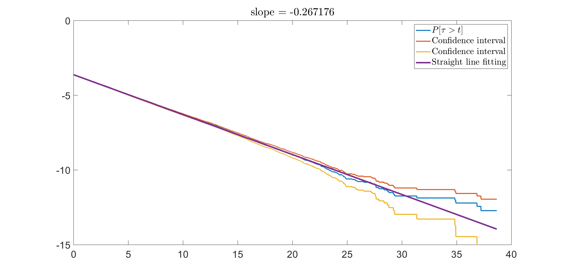
Figure 1. Plot of $\mathbb{P}(\tau>t)$ vs. $t$, confidence interval(upper bound and lower bound) and function $y=e^{-\lambda t}$

.

Furthermore, we would like to show the robustness of our data-driven QSD solver. The QSD is not explicit given so we use very large sample size ($10^{10}$ samples) and very small step size ($10^{-4}$) to obtain a much more accurate solution, which is served as the benchmark. Then we compare the numerical solutions obtained by the Monte Carlo method and the data-driven method for QSD with $N=10^{6}$ and $N=10^{8}$ samples, respectively. The result is shown in the first column of Figure 2. The data-driven solver performs much better than the Monte Carlo approximation for $N=10^{6}$ samples. It takes $10^{8}$ samples for the direct Monte Carlo sampler to produce a solution that looks as good as the QSD solver. Similar as the data-driven Fokker-Planck solver, our data-driven QSD solver can tolerate high level error in Monte Carlo simulation that has small spatial correlation.

It remains to check the effect of Brownian Bridge. We apply different time step sizes $\delta=0.01$ and $\delta=0.001$ for each trajectory. We use $10^{7}$ samples for $\delta=0.001$ and $10^{6}$ samples for $\delta=0.01$ to make sure that the number of killing events (for estimating the killing rate) are comparable. When $\delta=0.001$, the error is small with and without Brownian bridge correction. But Brownian bridge correction obviously improves the quality of solution when $\delta=0.01$. See the lower left panel of Figure 2. This is expected because, with larger time step size, the probability that the Brownian bridge hits the absorbing set $\partial\mathcal{X}$ gets higher.

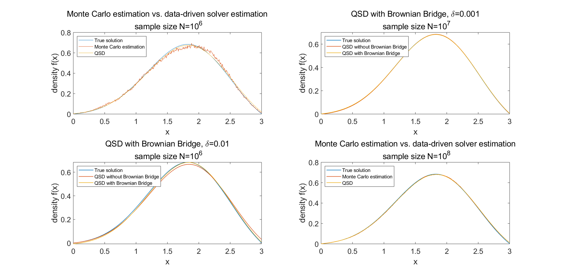
Figure 2. Left column: Monte Carlo estimation vs. data-driven solver estimation. Middle column: Effect of Brownian Bridge for sample size $N=10^{6}$ and $N=10^{8}$, with time step size 0.001. Right column: Effect of Brownian Bridge for sample size $N=10^{6}$ and $N=10^{8}$, with time step size 0.01.

5.2. Wright-Fisher Diffusion

The second numerical example is the Wright-Fisher diffusion model, which describes the evolution of colony undergoing random mating, possible under the additional actions of mutation and selection with or without dominance [11]. The Wright-Fisher model is an SDE

$$dX_{t}=-X_{t}dt+\sqrt{X_{t}(1-X_{t})}dW_{t},$$

where $W_{t}$ is a Wiener process and $\partial\mathcal{X}=\{0\}$ is the absorbing set. By the analysis of [11], the Yaglom limit, i.e., the QSD, satisfies

$$\lim_{t\rightarrow\infty}\mathbb{P}[X_{t}\in dy|\tau>t]=2(1-y)dy.$$

The goal of this example is to show the effect of Brownian bridge when the coefficient of noise is singular at the boundary. Since the Euler-Maruyama scheme only has an order of accuracy $0.5$, in the simulation, we apply the Milstein scheme, which reads

$$\hat{X}^{\delta}_{n+1}=\hat{X}^{\delta}_{n}-\hat{X}_{n}^{\delta}\delta+\sqrt{\hat{X}^{\delta}_{n}(1-\hat{X}^{\delta}_{n})}(W_{(n+1)\delta}-W_{n\delta})+\frac{1}{4}(1-2\hat{X}^{\delta}_{n})[(W_{(n+1)\delta}-W_{n\delta})^{2}-\delta]$$

One difficulty of using the Brownian bridge correction in this model is that the coefficient of the Brownian motion is vanishing at the boundary. Recall that the strength coefficient of Brownian bridge is denoted by $\phi$. Since the coefficient of the Brownian motion is vanishing, the original strength coefficient $\phi=\sqrt{\hat{X}_{n}^{\delta}(1-\hat{X}_{n}^{\delta})}$ can dramatically overestimate the probability of hitting the boundary. In this example, it is not possible to explicitly calculate the conditional distribution of the Brownian bridge that starts from $x:=\hat{X}_{n}^{\delta}$ and ends at $y:=\hat{X}_{n+1}^{\delta}$. But we find that empirically $\phi^{2}=\frac{1}{3}\min\{x(1-x),y(1-y)\}$ can fix this problem. Since a similar vanishing coefficient of the Brownian motion also appears in many ecological models, we will implement this modified Brownian bridge correction when simulating these models.

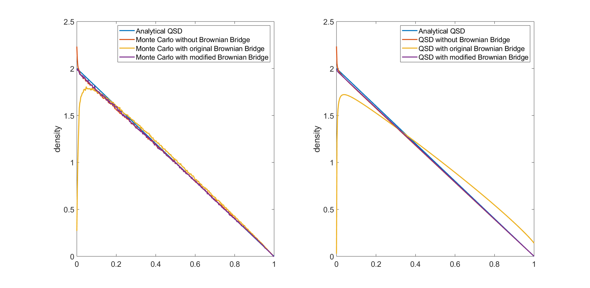
Figure 3. Effect of Brownian Bridge and a correction of Brownian Bridge. Left: Monte Carlo approximations without Brownian Bridge correction, with original Brownian Bridge correction, and with modified Brownian Bridge correction, in comparison to the analytical QSD. Right: Result from the data-driven QSD solver using the Monte Carlo simulation data from Left panel.

The effect of Brownian bridge is shown in the left side of Figure 3. We compare the solutions obtained via Monte Carlo method and the data-driven method with Brownian Bridge by running $10^{7}$ samples on $[0,1]$ with time step size $\delta=0.01$. The Monte Carlo approximation is far from the true density function of Beta(1,2) near $x=0$, while the use of the original Brownian Bridge only makes things worse. The modified Brownian Bridge solves this boundary effect problem reasonably well. The output of the data-driven QSD solver has a similar result (Figure 3 Right). Let $x=\hat{X}_{n}^{\delta}$ and $y=\hat{X}_{n+1}^{\delta}$. One can see that the numerical QSD is much closer to the true distribution if we replace the strength coefficient of the Brownian bridge $\phi^{2}=x(1-x)$ by the modified strength coefficient $\phi^{2}=\frac{1}{3}\min\{x(1-x),y(1-y)\}$.

5.3. Ring density function

Consider the following stochastic differential equation:

$$\begin{split}dX&=(-4X(X^{2}+X^{2}-1)+Y)dt+\epsilon dW^{x}_{t}\\ dY&=(-4X(X^{2}+Y^{2}-1)-X)dt+\epsilon dW^{y}_{t},\end{split}$$

where $W^{x}_{t}$ and $W^{y}_{t}$ are independent Wiener processes. In the simulation, we set the strength of noise $\epsilon=1$.

We first look at the approximation obtained by Monte Carlo method with $256\times 256$ mesh points on the domain $D=[-1.5,1.5]\times[-1.5,1.5]$. The simulation uses step size $\delta=0.001$ and $N=10^{8}$ samples. (See upper left panel in Figure 4). The Monte Carlo approximation has too much noise to be useful. The quality of this solution can be significantly improved by using the data-driven QSD solver. See upper right panel in Figure 4.

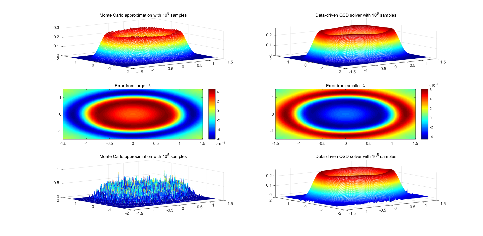
Figure 4. (Ring density) Upper panel:The approximation by Monte Carlo simulation(left) and the algorithm in Section 3.2(right) with $256\times 256$ mesh points and $10^{8}$ samples. Middle panel: Sensitivity effect of small change to killing rate $\lambda$. Lower panel: The approximation by Monte Carlo simulation with smaller samples(left) and the output of the data-driven QSD solver(right).

The simulation result shows the estimated rate of killing $\lambda=-0.176302$. We use this example to test the sensitivity of solution u against small change of the killing rate. We compare the approximations obtained by setting the killing rate be $\lambda$, $1.1\lambda$ and $0.9\lambda$ respectively. Heat maps of the difference between QSDs with “correct” and “wrong” killing rates are shown in two middle panels in Figure 4. It shows that difference brought by “wrong” rates is only $\approx O(10^{-4})$, which can be neglected. This result coincides with the analysis in Theorem 3.1 in this paper.

Finally, we would like to emphasis that the data-driven QSD solver can tolerate very high level of spatially uncorrelated noise in the reference solution $\mathbf{v}$. For example, if we use the same long trajectory with $10^{8}$ samples that generates the top left panel of Figure 4, but only select $10^{5}$ samples with intervals of $10^{3}$ steps of the numerical SDE solver, the Monte Carlo data becomes very noisy (Bottom left panel of Figure 4). However, longer intermittency between samples also reduces the spatial correlation between samples. As a result, the output of the QSD solver has very little change except at the boundary grid points, because the optimization problem (3.2) projects most of error to the boundary of the domain. (See bottom right panel of Figure 4.) This result highlights the need of high quality samplers. A Monte Carlo sampler with smaller spatial correlation between samples can significantly reduce the number of samples needed in the data-driven QSD solver.

5.4. Sensitivity of QSD: 1D examples

In this subsection, we use 1D examples to study the sensitivity of QSDs against changes on boundary conditions. Consider an 1D gradient flow of the potential function $V(x)$ with an additive noise perturbation

(5.2) $$X_{t}=-V^{\prime}(X_{t})dt+\sigma dW_{t}.$$

Let $(-\infty,0]$ be the absorbing state of $X_{t}$. So if $V(0)<\infty$, $X_{t}$ admits a QSD, denoted by $\mu_{X}$. If we let the stochastic process reflect at $x=0$, the modified stochastic process, denoted by $Y_{t}$, admits an invariant probability measure denoted by $\mu_{Y}$. We will compare the sensitivity of $\mu_{X}$ against the change of boundary condition for two different cases whose speed of mixing are different, namely a single well potential function and a double well potential function.

We choose a single well potential function $V_{1}(x)=(x-1)^{2}$ and a double well potential function $V_{2}(x)=x^{4}-4\sqrt{2}x^{3}+10x^{2}-4\sqrt{2}x+1$. The values of minima of both $V_{1}$ and $V_{2}$ are zero. The values of $V_{1}$ and $V_{2}$ at the absorbing state are $1$. And the height of the barrier between two local minima of $V_{2}$ is $1$. The strength of noise is $\sigma=0.7$ in both examples. See Figure 5 middle column for plots of these two potential functions. In both cases, the QSD and the invariant probability measure are computed on the domain $D=[0,3]$. To further distinguish these two cases, we denote the QSD of equation (5.2) with absorbing state $x=0$ and potential function $V_{1}(x)$ (resp. $V_{2}(x)$) by $\mu_{X}^{1}$ (resp. $\mu_{X}^{2}$) and the invariant probability measure of equation (5.2) with reflection boundary at $(-\infty,0]$ and potential function $V_{1}(x)$ (resp. $V_{2}(x)$) by $\mu_{Y}^{1}$ (resp. $\mu_{Y}^{2}$). Probability measures $\mu_{X}^{1}$ and $\mu_{Y}^{1}$ (resp. $\mu_{X}^{2}$ and $\mu_{Y}^{2}$) are compared in Figure 5 right column. We can see that the QSD and the invariant probability measure have small difference for the single well potential function $V_{1}$. But they look very different for the double well potential function $V_{2}$. With the double well potential function, there is a visible difference between probability density functions of $\mu^{2}_{X}$ and $\mu^{2}_{Y}$. The density function of QSD is much smaller than the invariant probability measure around the left local minimum $x=1-\sqrt{2}$ because this local minimum is closer to the absorbing set, which makes killing and regeneration more frequent when $X_{t}$ is near this local minimum. In other words, the QSD of equation (5.2) with respect to the double well potential is very sensitive against the change at the boundary.

The reason of the high sensitivity is illustrated by the coupling argument. We first run Algorithm 3 with 8 independent long trajectories with length of $10^{6}$ and collect the coupling times. The slope of exponential tail of the coupling time gives the rate of contraction of $P^{T}_{Y}$. The $\mathbb{P}(\tau^{C}>t)$ versus $t$ plot is demonstrated in log-linear plot in Figure 5 left column. The slope of exponential tail is $\gamma=2.031414$ for the single well potential $V_{1}$, and $\gamma=0.027521$ for the double well potential case. Then we run Algorithm 4 to estimate the finite time error $\mathrm{d}_{w}(\mu_{X}P_{X}^{T},\mu_{X}P_{Y}^{T})$ for both cases. Since the single well potential case has a much faster coupling speed, we can choose $T=0.5$. The output of Algorithm 4 is $d_{w}(\mu_{X}P^{T}_{X},\mu_{X}P^{T}_{Y})\approx 0.00391083$. This gives an estimate $d_{w}(\mu_{X},\mu_{Y})\approx 0.0061$. The double well potential case converges much slower. We choose $T=20$ to make sure that the denominator $1-e^{-\gamma T}$ is not too small. As a result, Algorithm 4 gives an approximation $d_{w}(\mu_{X}P^{T}_{X},\mu_{X}P^{T}_{Y})\approx 0.06402$, which means $d_{w}(\mu_{X},\mu_{Y})\approx 0.1512$. This is consistent with the right column seen in Figure 5, the QSD of the double well potential is much more sensitive against a change of the boundary condition than the single well potential case.

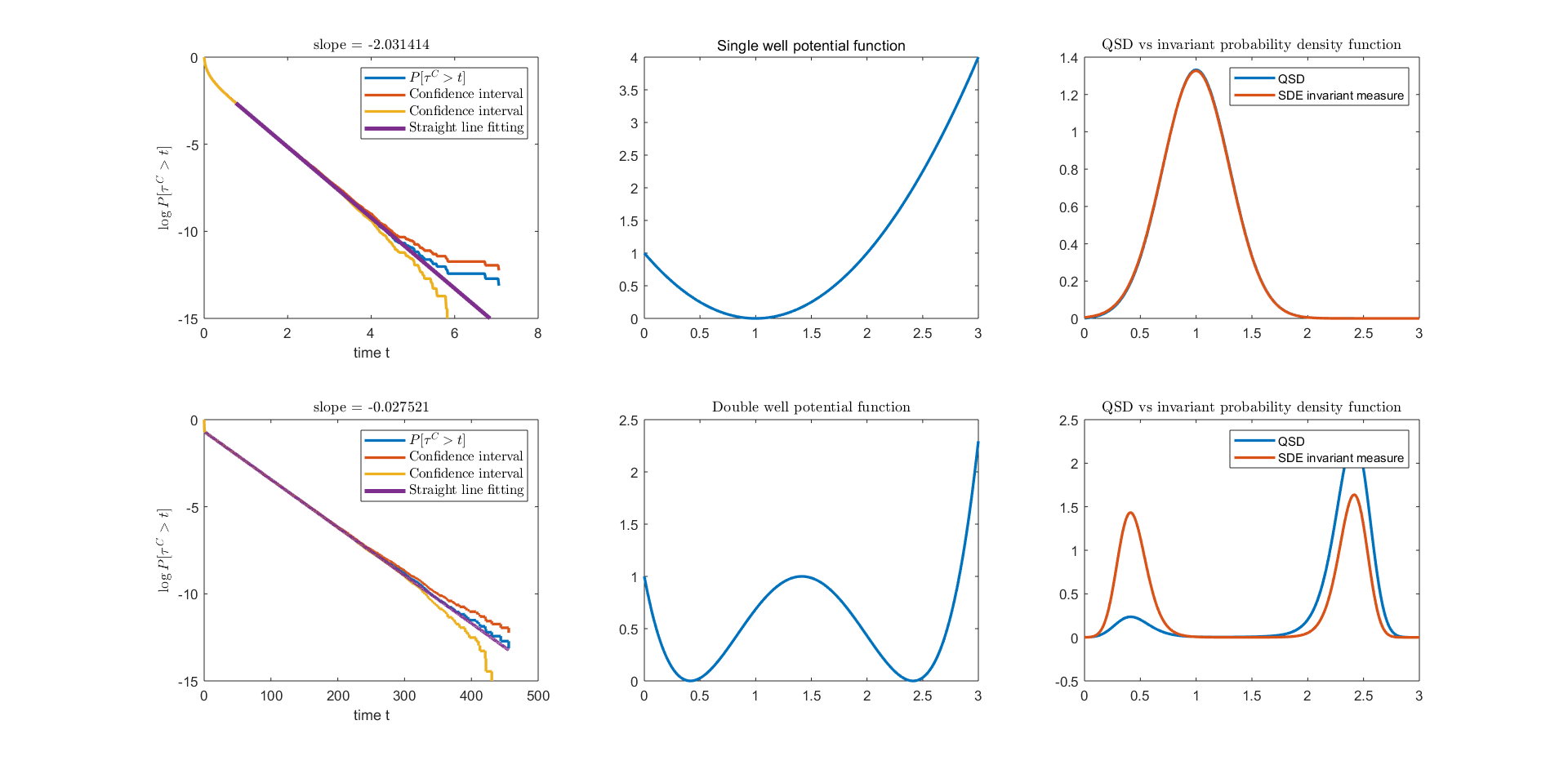
Figure 5. (Single well vs. Double well potential function) Left column: $\mathbb{P}(\tau^{C}>t)$ vs. $t$. Middle column: Single well and double well potential functions. Right column: QSD vs. invariant density function.

5.5. Lotka-Volterra Competitive Dynamics

In this example, we focus on the effect of demographic noise on the classical Lotka-Volterra competitive system. The Lotka-Volterra competitive system with some environmental fluctuation has the form

(5.3) $$\begin{split}dY_{1}(t)&=Y_{1}(t)(l_{1}-a_{11}Y_{1}(t)-a_{12}Y_{2}(t))dt+\sigma^{\prime}_{1}Y_{1}(t)dW_{1}(t),\\ dY_{2}(t)&=Y_{2}(t)(l_{2}-a_{22}Y_{1}(t)-a_{21}Y_{1}(t))dt+\sigma^{\prime}_{2}Y_{2}(t)dW_{2}(t).\end{split}$$

Here $l_{i}>0$ is the per-capita growth rate of species $i$ and $a_{ij}>0$ is the per-capita competition rate between species $i$ and $j$. More details can be found in [10]. Model parameters are chosen to be $l_{1}=2,l_{2}=4,a_{11}=0.8,a_{12}=1.6,a_{21}=1,a_{22}=5$. Let $\partial\mathcal{X}$ be the union of x-axis and y-axis. For suitable $\sigma^{\prime}_{1}$ and $\sigma^{\prime}_{2}$, $Y_{1}$ and $Y_{2}$ can coexist such that the probability of $(Y_{1},Y_{2})$ hits $\partial\mathcal{X}$ in finite time is zero. So equation (5.3) admits an invariant probability measure, denoted by $\mu_{Y}$.

As a modification, we add a small demographic noise term to equation (5.4). The equation becomes

(5.4) $$\begin{split}dX_{1}(t)&=X_{1}(t)(l_{1}-a_{11}X_{1}(t)-a_{12}X_{2}(t))dt+\sigma_{1}X_{1}(t)dW_{1}(t)+\epsilon\sqrt{X_{1}(t)}dW^{\prime}_{1}(t),\\ dX_{2}(t)&=X_{2}(t)(l_{2}-a_{22}X_{1}(t)-a_{21}X_{1}(t))dt+\sigma_{2}X_{2}(t)dW_{2}(t)+\epsilon\sqrt{X_{2}(t)}dW^{\prime}_{2}(t).\end{split}$$

It is easy to see that equation (5.4) can exit to the boundary $\partial\mathcal{X}$. It admits a QSD, denoted by $\mu_{X}$.

In order to study the effect of demographic noise, we compare $\mu_{Y}$, the numerical invariant measure of equation (5.3), and $\mu_{X}$, the QSD of equation (5.4). In our simulation, we fix the strength of demographic noise as $\epsilon=0.05$ and compare $\mu_{X}$ and $\mu_{Y}$ at two different levels of the environment noise $\sigma_{1}=\sigma_{2}=0.75$ and $\sigma_{1}=\sigma_{2}=1.1$ respectively. The coefficient $\sigma_{1}^{\prime}$ and $\sigma_{2}^{\prime}$ in equation (5.3) satisfies $\sigma_{i}^{\prime}=\sqrt{\sigma_{i}^{2}+\epsilon^{2}}$ for $i=1,2$ to match the effect of the additional demographic noise. Compare Figure 6 and Figure 7, one can see that $\mu_{Y}$ has significant concentration at the boundary when $\sigma_{1}=\sigma_{2}=1.1$.

The result for $\sigma_{1}=\sigma_{2}=0.75$ is shown in Figure 6. Left bottom of Figure 6 shows the invariant measure. The QSD is shown on right top of Figure 6. The total variation distance between these two measures are shown at the bottom of Figure 6. The difference is very small and it just appears around boundary. This is reasonable because with high probability, the trajectories of equation (5.4) moves far from the absorbing set $\partial\mathcal{X}$ in both cases, which makes the regeneration events happen less often. This is consistent with the result of Lemma 4.2. We compute the distribution of the coupling time. The coupling time distribution and its exponential tail are shown in Figure 6 Top Left. Then we use Algorithm 5 to compute the finite time error. To better match two trajectories given by equations (5.3) and (5.4), we separate the noise term in equation (5.3) into $\sigma_{i}^{\prime}Y_{i}(t)\mathrm{d}W_{i}(t)=\sigma_{i}Y_{i}(t)\mathrm{d}W^{(1)}_{i}(t)+\epsilon Y_{i}(t)\mathrm{d}W^{(2)}_{i}(t)$ for $i=1,2$, where $W^{(1)}_{i}(t)$ and $W^{(2)}_{i}(t)$ use the same Wiener process trajectory as $W_{i}(t)$ and $W^{\prime}_{i}(t)$ in equation (5.4) for $i=1,2$. Let $T=4$. The finite time error caused by the demographic noise is $0.01773$. As a result, the upper bound given in Lemma 4.2 is $0.02835$. Note that as seen in Figure 6, this upper bound actually significantly overestimates the distance between the invariant probability measure and the QSD. The empirical total variation distance is much smaller that our theoretical upper bound. This is because the way of matching $\sigma^{\prime}_{i}Y_{i}\mathrm{d}W_{i}(t)$ and $\sigma_{i}X_{i}(t)\mathrm{d}W_{i}(t)+\epsilon\sqrt{X_{i}(t)}\mathrm{d}W_{i}(t)$ is very rough. A better approach of matching those noise terms will likely lead to a more accurate estimation of the upper bound of the error.

The results for $\sigma_{1}=\sigma_{2}=1.1$ are shown in Figure 7. The total variation distance between these two measures are shown at the bottom of Figure 7. It is not hard to see the difference is significantly larger than case $\sigma=0.75$. The reason is that trajectories of equation (5.4) have high probability moving along the boundary in this parameter setting. This makes the probability of falling into the absorbing set $\partial\mathcal{X}$ much higher. Same as above, we compute the distribution of the coupling time and demonstrate the coupling time distribution (as well as the exponential tail) in Figure 7 Top Left. The coupling in this example is slower so we choose $T=12$ to run Algorithm 5. The probability of killing before $T$ is approximately $0.11186$ and the total finite time error caused by the demographic noise is $0.06230$. As a result, the upper bound given in Lemma 4.2 is $0.1356$. This is consistent with the numerical finding shown in Figure 7 Bottom Right.

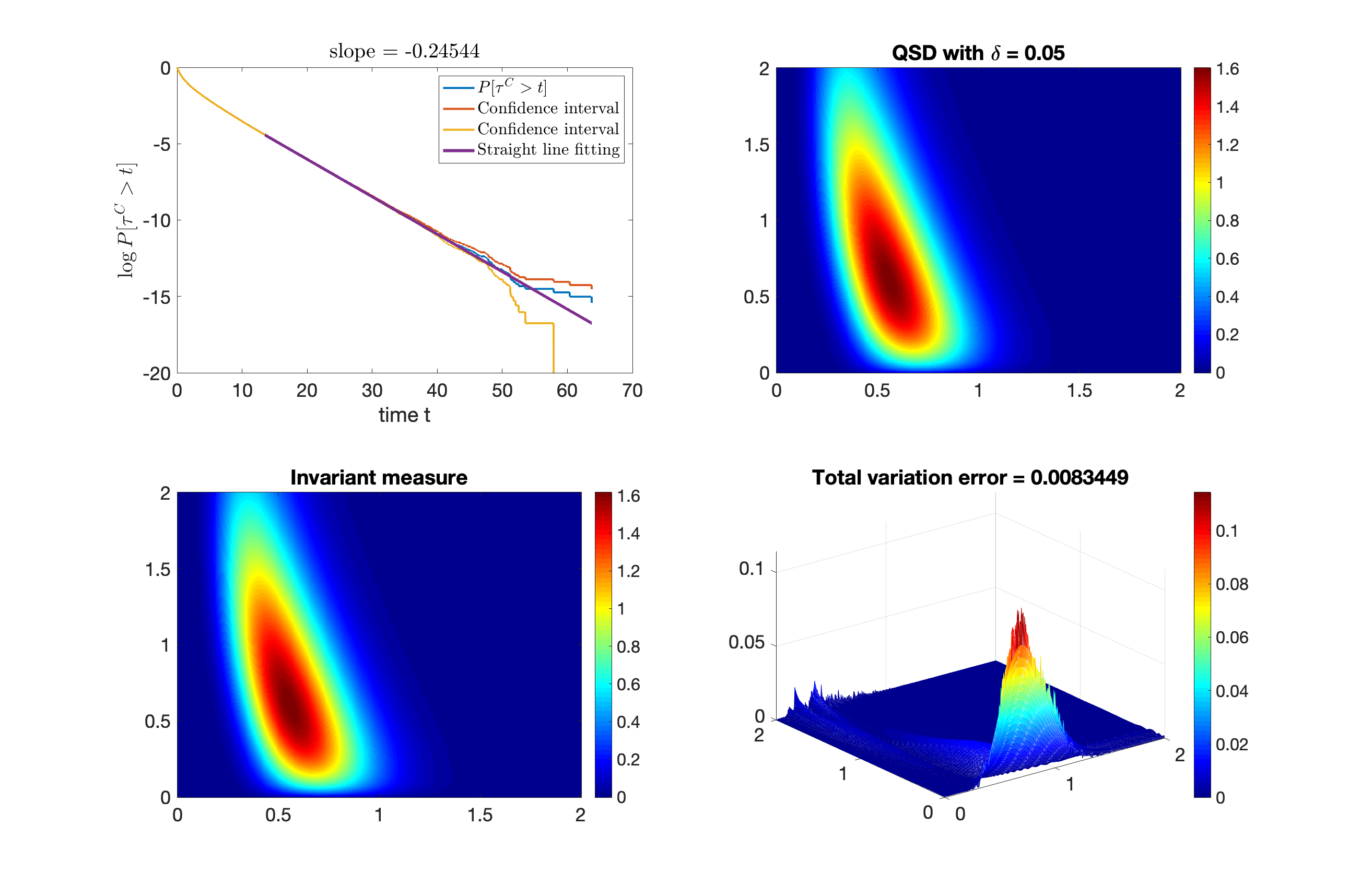
Figure 6. (Case $\sigma_{1}=\sigma_{2}=0.75$) Upper panel: (Left) $\mathbb{P}(\tau^{C}>t)$ vs.$t$. (Right) QSD with demographic noise coefficient $\epsilon=0.05$. Lower panel: (Left) Invariant density function for $\sigma=0.75$. (Right) Total variation of QSD and invariant density function.

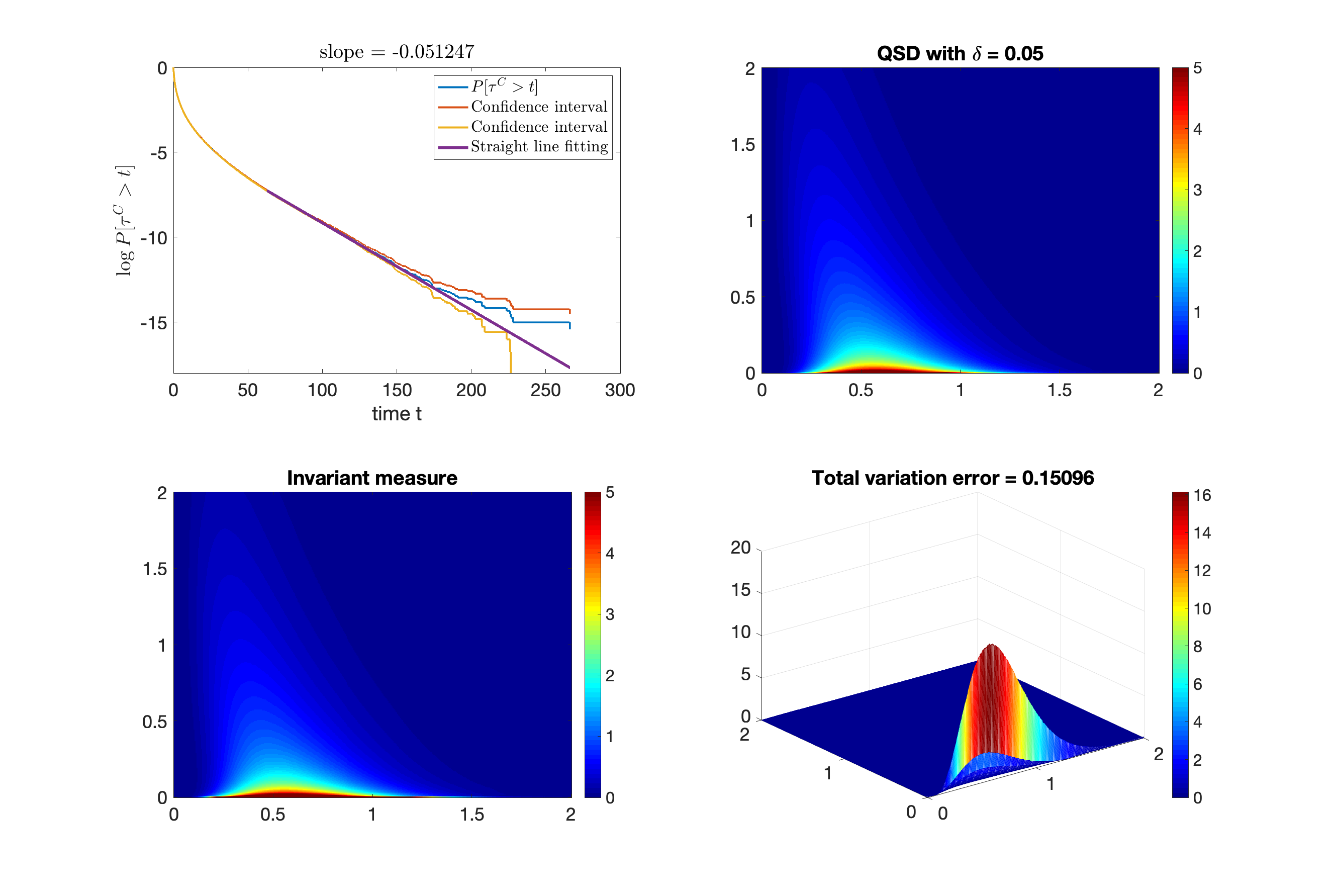
Figure 7. (Case $\sigma_{1}=\sigma_{2}=1.1$) Upper panel: (Left) $\mathbb{P}(\tau^{C}>t)$ vs.$t$. (Right) QSD with demographic noise coefficient $\epsilon=0.05$. Lower panel: (Left) Invariant density function for $\sigma=1.1$. (Right) Total variation of QSD and invariant density function.

5.6. Chaotic attractor

In this subsection, we consider a non-trivial 3D example that has interactions between chaos and random perturbations, called the Rossler oscillator. The random perturbation of the Rossler oscillator is

(5.5) $$\begin{cases}dx=(-y-z)dt+\epsilon dW^{x}_{t}\\ dy=(x+ay)dt+\epsilon dW^{y}_{t}\\ dz=(b+z(x-c))dt+\epsilon dW^{z}_{t},\end{cases}$$

where $a=0.2,b=0.2,c=5.7$, and $W^{x}_{t},W^{y}_{t}$ and $W^{z}_{t}$ are independent Wiener processes. The strength of noise is chosen to be $\epsilon=0.1$. This system is a representative example of chaotic ODE systems appearing in many applications of physics, biology and engineering. We consider equation (5.5) restricted to the box $D=[-15,15]\times[-15,15]\times[-1.5,1.5]$. Therefore, it admits a QSD supported by $D$. In this example, a grid with $1024\times 1024\times 128$ mesh points is constructed on $D$.

It is very difficult to use traditional PDE solver to compute a large scale 3D problem. To analyze the QSD of this chaotic system, we apply the blocked version of the Fokker-Planck solver studied in [7]. More precisely, a big mesh is divided into many “blocks”. Then we solve the optimization problem (3.2) in parallel. The collaged solution is then processed by the “shifting block” technique to reduce the interface error, which means the blocks are reconstructed such that the center of new blocks cover the boundary of old blocks. Then we let the solution from the first found serve as the reference data, and solve optimization problem (3.2) again based on new blocks. See [7] for the full details of implementation. In this example, the grid is further divided into $32\times 32\times 4$ blocks. We run the “shifting block” solver for 3 repeats to eliminate the interface error. The reference solution is generated by a Monte Carlo simulation with $10^{9}$ samples. The killing rate is $\lambda=-0.473011$. Two “slices” of the solution, as seen in Figure 8, are then projected to the xy-plane for the sake of easier demonstration. See the caption of Figure 8 for the coordinates of these two “slices”. The left picture in Figure 8 shows the projection of the solution has both dense and sparse parts that are clearly divided. An outer ”ring” with high density appears and the density decays quickly outside this ”ring.” The right picture in Figure 8 demonstrates the solution has much lower density when $z$-coordinate is larger than 1.

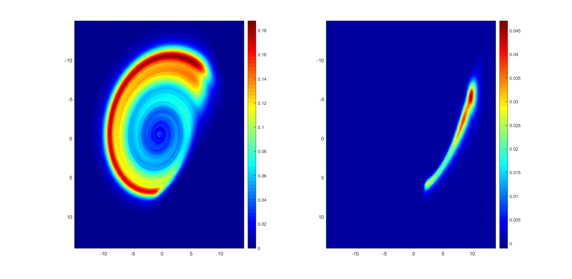
Figure 8. (Rossler) Projections of 2 ”slices” of the QSD of the Rossler system to the xy-plane. z-coordinates of 2 slices are [-0.0352, 0.2578], [1.1367, 1.4297]. The solution is obtained by a balf-block shift solver on $[-15,15]\times[-15,15]\times[-1.5,1.5]$ with $1024\times 1024\times 128$ mesh points, $32\times 32\times 4$ blocks, and $10^{9}$ samples.

6. Conclusion

In this paper we provide some data-driven methods for the computation of quasi-stationary distributions (QSDs) and the sensitivity analysis of QSDs. Both of them are extended from the first author’s earlier work about invariant probability measures. When using the Fokker-Planck equation to solve the QSD, we find that the idea of using a reference solution with low accuracy to set up an optimization problem still works well for QSDs. And the QSD is not very sensitively dependent on the killing rate, which is given by the Monte Carlo simulation when producing the reference solution. The data-driven Fokker-Planck solver studied in this paper is still based on discretization. But we expect the mesh-free Fokker-Planck solver proposed in [7] to work for solving QSDs. In the sensitivity analysis part, the focus is on the relation between a QSD and the invariant probability measure of a “modified process”, because many interesting problems in applications fall into this category. The sensitivity analysis needs both a finite time truncation error and a contraction rate of the Markov transition kernel. The approach of estimating the finite time truncation error is standard. The contraction rate is estimated by using the novel numerical coupling approach developed in [17]. The sensitivity analysis of QSDs can be extended to other settings, such as the sensitivity against small perturbation of parameters, or the sensitivity of a chemical reaction process against its diffusion approximation. We will continue to study sensitivity analysis related to QSDs in our subsequent work.

References

- [1] Alan Agresti and Brent A Coull. Approximate is better than “exact” for interval estimation of binomial proportions. The American Statistician, 52(2):119–126, 1998.
- [2] William J Anderson. Continuous-time Markov chains: An applications-oriented approach. Springer Science & Business Media, 2012.
- [3] Russell R Barton and Lee W Schruben. Uniform and bootstrap resampling of empirical distributions. In Proceedings of the 25th conference on Winter simulation, pages 503–508, 1993.
- [4] Michel Benaim, Bertrand Cloez, Fabien Panloup, et al. Stochastic approximation of quasi-stationary distributions on compact spaces and applications. Annals of Applied Probability, 28(4):2370–2416, 2018.
- [5] Pierre Collet, Servet Martínez, and Jaime San Martín. Quasi-stationary distributions: Markov chains, diffusions and dynamical systems. Springer Science & Business Media, 2012.
- [6] John N Darroch and Eugene Seneta. On quasi-stationary distributions in absorbing discrete-time finite markov chains. Journal of Applied Probability, 2(1):88–100, 1965.
- [7] Matthew Dobson, Yao Li, and Jiayu Zhai. An efficient data-driven solver for fokker-planck equations: algorithm and analysis. arXiv preprint arXiv:1906.02600, 2019.
- [8] Matthew Dobson, Yao Li, and Jiayu Zhai. Using coupling methods to estimate sample quality of stochastic differential equations. SIAM/ASA Journal on Uncertainty Quantification, 9(1):135–162, 2021.
- [9] Pablo A Ferrari, Servet Martínez, and Pierre Picco. Existence of non-trivial quasi-stationary distributions in the birth-death chain. Advances in applied probability, pages 795–813, 1992.
- [10] Alexandru Hening and Yao Li. Stationary distributions of persistent ecological systems. arXiv preprint arXiv:2003.04398, 2020.
- [11] Thierry Huillet. On wright–fisher diffusion and its relatives. Journal of Statistical Mechanics: Theory and Experiment, 2007(11):P11006, 2007.
- [12] James E Johndrow and Jonathan C Mattingly. Error bounds for approximations of markov chains used in bayesian sampling. arXiv preprint arXiv:1711.05382, 2017.
- [13] Ioannis Karatzas and Steven Shreve. Brownian motion and stochastic calculus, volume 113. springer, 2014.
- [14] Peter E Kloeden and Eckhard Platen. Stochastic differential equations. In Numerical Solution of Stochastic Differential Equations, pages 103–160. Springer, 1992.
- [15] Ying-Cheng Lai and Tamás Tél. Transient chaos: complex dynamics on finite time scales, volume 173. Springer Science & Business Media, 2011.
- [16] Yao Li. A data-driven method for the steady state of randomly perturbed dynamics. arXiv preprint arXiv:1805.04099, 2018.
- [17] Yao Li and Shirou Wang. Numerical computations of geometric ergodicity for stochastic dynamics. Nonlinearity, 33(12):6935, 2020.
- [18] Bernt Øksendal. Stochastic differential equations. In Stochastic differential equations, pages 65–84. Springer, 2003.
- [19] Christian Robert and George Casella. Monte Carlo statistical methods. Springer Science & Business Media, 2013.
- [20] Erik A Van Doorn. Quasi-stationary distributions and convergence to quasi-stationarity of birth-death processes. Advances in Applied Probability, pages 683–700, 1991.
- [21] Erik A van Doorn and Pauline Schrijner. Geomatric ergodicity and quasi-stationarity in discrete-time birth-death processes. The ANZIAM Journal, 37(2):121–144, 1995.