Approximation Algorithms for Orthogonal Non-negative Matrix Factorization

Abstract

In the non-negative matrix factorization (NMF) problem, the input is an $m\times n$ matrix $M$ with non-negative entries and the goal is to factorize it as $M\approx AW$. The $m\times k$ matrix $A$ and the $k\times n$ matrix $W$ are both constrained to have non-negative entries. This is in contrast to singular value decomposition, where the matrices $A$ and $W$ can have negative entries but must satisfy the orthogonality constraint: the columns of $A$ are orthogonal and the rows of $W$ are also orthogonal. The orthogonal non-negative matrix factorization (ONMF) problem imposes both the non-negativity and the orthogonality constraints, and previous work showed that it leads to better performances than NMF on many clustering tasks. We give the first constant-factor approximation algorithm for ONMF when one or both of $A$ and $W$ are subject to the orthogonality constraint. We also show an interesting connection to the correlation clustering problem on bipartite graphs. Our experiments on synthetic and real-world data show that our algorithm achieves similar or smaller errors compared to previous ONMF algorithms while ensuring perfect orthogonality (many previous algorithms do not satisfy the hard orthogonality constraint).

1 Introduction

Low-rank approximation of matrices is a fundamental technique in data analysis. Given a large data matrix $M$ of size $m\times n$, the goal is to approximate it by a low-rank matrix $AW$ where $A$ has size $m\times k$ and $W$ has size $k\times n$. Here $k$ is called the inner dimension of the factorization $M\approx AW$, controlling the rank of $AW$. Such low-rank matrix decomposition enables a succinct and often more interpretable representation of the original data matrix $M$.

One of the standard approaches of low-rank approximation is singular value decomposition (SVD) (Wold et al., 1987; Alter et al., 2000; Papadimitriou et al., 2000). SVD computes a solution minimizing both the Frobenius norm $\|M-AW\|_{F}$ and the spectral norm $\sigma_{\textnormal{max}}(M-AW)$ (Eckart and Young, 1936; Mirsky, 1960). In addition, SVD always gives a solution with the orthogonality property: the columns of $A$ are orthogonal and the rows of $W$ are also orthogonal. Orthogonality makes the factors more separable, and thus causes the low-rank representation to have a cleaner structure.

However, in certain cases the data matrix $M$ is inherently non-negative, with entries corresponding to frequencies or probability mass, and in these cases SVD has a serious limitation: the factors $A$ and $W$ computed by SVD often contain negative entries, making the factorization less interpretable. Non-negative matrix factorization (NMF), which constrains $A$ and $W$ to have non-negative entries, is better suited to these cases, and is applied in many domains including computer vision (Lee and Seung, 1999; Li et al., 2001), text mining (Xu et al., 2003; Pauca et al., 2004) and bioinformatics (Brunet et al., 2004; Kim and Park, 2007; Devarajan, 2008).

One drawback of NMF relative to SVD is that it gives less separable factors: the angle between any two columns of $A$ or any two rows of $W$ is at most $\pi/2$ simply because the inner product of a pair of vectors with non-negative coordinates is always non-negative. To reap the benefits of non-negativity and orthogonality simultaneously, orthogonal NMF (ONMF) adds orthogonality constraints to NMF on one or both of the factors $A$ and $W$: the columns of $A$ and/or the rows of $W$ are required to be orthogonal. Indeed, ONMF leads to better empirical performances in many clustering tasks (Ding et al., 2006; Choi, 2008; Yoo and Choi, 2010). While previous works showed ONMF algorithms that converge to local minima (Ding et al., 2006) and an efficient polynomial-time approximation scheme (EPTAS) assuming the inner-dimension is a constant (Asteris et al., 2015), a theoretical understanding of the worst-case guarantee one can achieve for ONMF with arbitrary inner-dimension is lacking. In this work, we show the first constant-factor approximation algorithm for ONMF with respect to the squared Frobenius error $\|M-AW\|_{F}^{2}$ when the orthogonality constraint is imposed on one or both of the factors.

Our Results

We use approximation algorithms for weighted $k$-means as subroutines, such as the $(9+\varepsilon)$-approximation local search algorithm by Kanungo et al. (2002). Assuming an $r$-approximation algorithm for weighted $k$-means, we show algorithms for ONMF with approximation ratio $2r$ in the single-factor orthogonality setting where only one of the factors $A$ or $W$ is required to be orthogonal (Theorem 3), and approximation ratio $\left(2r+\frac{8r+8}{\sin^{2}(\pi/12)}\right)$ in the double-factor orthogonality setting where both $A$ and $W$ are required to be orthogonal (Theorem 8). Here, $A$ (resp. $W$) being orthogonal means that its columns (resp. rows) are orthogonal but not necessarily of unit length. The approximation ratios are provable upper bounds for the ratio between the error of the output $(A,W)$ of the algorithm and the minimum error over all feasible solutions $(A,W)$, with error measured using the squared Frobenius norm $\|M-AW\|_{F}^{2}$. We also demonstrate the superior practical performance of our algorithms by experiments in both the single-factor and the double-factor orthogonality setting on synthetic and real-world datasets (see Section 5 and Appendix G).

Sparse Structure of Solution

When we impose the orthogonality constraint on both the columns of $A$ and the rows of $W$, the non-negativity and the orthogonality constraints together cause the solution to ONMF to have a very sparse structure. Let ${\bm{a}}_{i}$ denote the $i$-th column of $A$ and ${\bm{w}}_{i}^{\mathsf{T}}$ denote the $i$-th row of $W$. Since ${\bm{a}}_{i}$ and ${\bm{a}}_{j}$ are constrained to have non-negative entries but zero inner product, they have disjoint supports, and this also holds for ${\bm{w}}_{i}$ and ${\bm{w}}_{j}$. As a result, $AW=\sum_{i=1}^{k}{\bm{a}}_{i}{\bm{w}}_{i}^{\mathsf{T}}$ naturally consists of $k$ disjoint blocks, as shown in Figure 1.

If the input $M$ factorizes as $M=AW$ exactly, we can easily recover $A$ and $W$ based on the block-wise structure of $M$. Therefore, we focus on the agnostic setting where $M=AW$ does not hold exactly, and design approximation algorithms that find solutions comparable to the best possible factorization.

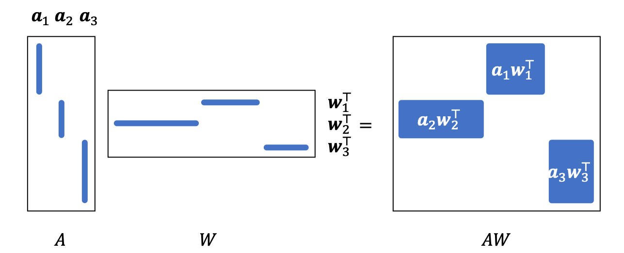
Figure 1: The $k$ columns of $A$ have disjoint supports. The $k$ rows of $W$ also have disjoint supports. The product $AW$ has entries equal to zero outside the $k$ blocks.

Connection to Bipartite Correlation Clustering

The block-wise structure of $AW$ (Figure 1) relates ONMF to the correlation clustering problem (Bansal et al., 2004) on complete bipartite graphs.

To see the relationship with correlation clustering, let us consider a data matrix $M$ with binary entries and assume $k\geq\min\{m,n\}$. Since we can find at most $\min\{m,n\}$ non-zero ${\bm{a}}_{i}{\bm{w}}_{i}^{\mathsf{T}}$ satisfying the orthogonal constraint, all $k\geq\min\{m,n\}$ give equivalent problems, where any inner-dimension is considered feasible. $M$ can be treated as a complete bipartite graph with vertices $\{u_{1},\ldots,u_{m}\}\cup\{v_{1},\ldots,v_{n}\}$ and edges $(u_{i},v_{j})$ labeled “$+$” if $M_{ij}=1$ or “$-$” if $M_{ij}=0$. This edge-labeled complete bipartite graph is exactly an instance of the correlation clustering problem. If the factors $A$ and $W$ also have binary entries and both satisfy the orthogonality constraint, the blocks of $AW=\sum_{i=1}^{k}{\bm{a}}_{i}{\bm{w}}_{i}^{\mathsf{T}}$ (see Figure 1) are all-ones matrices corresponding to vertex-disjoint complete bipartite sub-graphs. This is exactly the form of a solution to the correlation clustering problem, and the objective $\|M-AW\|_{F}^{2}$ is exactly the number of disagreements in the correlation clustering problem. Although our algorithm (specifically, the algorithm in Theorem 9) doesn’t impose the binary constraint on $A$ and $W$, we can apply the following lemma to each block of $AW$ to round the solution to binary with only a constant loss in the objective (see Appendix A for proof):

Lemma 1.

Let $M\in\{0,1\}^{m\times n}$ be a binary matrix. Let ${\bm{a}}\in\mathbb{R}^{m}_{\geq 0}$ and ${\bm{w}}\in\mathbb{R}^{n}_{\geq 0}$ be two non-negative vectors. Then, there exist binary vectors $\hat{\bm{a}}\in\{0,1\}^{m}$ and $\hat{\bm{w}}\in\{0,1\}^{n}$ such that

$$\|M-\hat{\bm{a}}\hat{\bm{w}}^{\mathsf{T}}\|_{F}^{2}\leq 8\|M-{\bm{a}}{\bm{w}}^{\mathsf{T}}\|_{F}^{2}.$$

Moreover, $\hat{\bm{a}}$ and $\hat{\bm{w}}$ can be computed in poly-time.

Thus, we can obtain an approximation algorithm for minimizing disagreements in complete bipartite graphs via our approximation algorithm for ONMF in Theorem 9. Moreover, without the binary constraint on $M,A,W$, ONMF with orthogonality constraint on both $A$ and $W$ can be treated as a soft version of bipartite correlation clustering.

Open Questions

We used the Frobenius norm as a natural measure of goodness of fit, but it would be interesting to see if one can achieve constant-factor approximation with respect to other measures, such as the spectral norm, since the two norms can be different by a factor that grows with $\min\{m,n\}$. It would also be interesting to consider replacing the orthogonality constraint on $A$ and $W$ by a lower bound $\theta<\pi/2$ on the angles between different columns of $A$ and different rows of $W$.

Related Work

Non-negative matrix factorization was first proposed by Paatero and Tapper (1994), and was shown to be NP-hard by Vavasis (2010). Algorithmic frameworks for efficiently finding local optima include the multiplicative updating framework (Lee and Seung, 2001) and the alternating non-negative least squares framework (Lin, 2007; Kim and Park, 2011). Under the usually mild separability assumption, Arora et al. (2016) showed an efficient algorithm that computes the global optimum.

Ding et al. (2006) first studied NMF with the orthogonality constraint, and showed its effectiveness in document clustering. After that, algorithms for ONMF using various techniques have been developed for a broad range of applications (Chen et al., 2009; Ma et al., 2010; Kuang et al., 2012; Pompili et al., 2013; Li et al., 2014b; Kim et al., 2015; Qin et al., 2016; Alaudah et al., 2017; Huang et al., 2019). The less restrictive single-factor orthogonality setting attracted the most attention, and most algorithms for solving it belong to the multiplicative updating framework: iteratively updating $A$ and/or $W$ by taking the element-wise product with other computed non-negative matrices (Yang and Laaksonen, 2007; Choi, 2008; Yoo and Choi, 2008, 2010; Yang and Oja, 2010; Pan and Ng, 2018; He et al., 2020). Other techniques include HALS (hierarchical alternating least squares) (Li et al., 2014a; Kimura et al., 2016) and using a penalty function (Del Buono, 2009) for the orthogonality constraint.

While improving the separability of the factors compared to NMF, these algorithm do not guarantee convergence to a solution that has perfect orthogonality (which is also demonstrated in our experiments). There are only a few previous algorithms that have this guarantee, including the EM-ONMF algorithm (Pompili et al., 2014), the ONMFS algorithm (Asteris et al., 2015) and the NRCG-ONMF algorithm Zhang et al. (2016). ONMFS is the only previous algorithm we know that has a provable approximation guarantee, but it has a running time exponential in the squared inner dimension. (Pompili et al., 2014) give a reduction of ONMF to spherical $k$-means with a somewhat non-standard objective function: the goal is to minimize the sum of $1$ minus the square of cosine similarity, while the commonly studied objective function for spherical $k$-means sums up $1$ minus the cosine similarity. Our results for ONMF imply a constant factor approximation for this variant of spherical $k$-means with the squared cosine similarity in the objective. Many variants of ONMF have also been studied in the literature, including the semi-ONMF (Li et al., 2018) and the sparse ONMF (Chen et al., 2018; Li et al., 2020).

We would also like to point out that the connection between ONMF and $k$-means shown in (Ding et al., 2006, Theorems 1 and 2) does not give a reduction in either direction. Their proof shows that the optimization problem associated with $k$-means is essentially ONMF, but with additional constraints: the matrix $G$ in the ONMF formulation (8) in (Ding et al., 2006) is replaced by matrix $\tilde{G}$ in the $k$-means formulation (11) in (Ding et al., 2006). However $\tilde{G}$ is a “normalized cluster indicator matrix” that is more constrained than the generic matrix $G$ with orthonormal columns because the entries in every column of $\tilde{G}$ are either zero or take the same non-zero value. This additional constraint makes their argument insufficient to either directly derive an algorithm for ONMF with the same approximation guarantee given one for $k$-means, or the other way around. Also, later works such as Yoo and Choi (2010) and Asteris et al. (2015) used techniques different from $k$-means to improve the empirical performance of ONMF.

The correlation clustering problem was proposed by Bansal et al. (2004) on complete graphs, who showed a constant factor approximation algorithm for the disagreement minimization version and a polynomial-time approximation scheme (PTAS) for the agreement maximization version. Ailon et al. (2008) showed a simple combinatorial algorithm achieving an approximation ratio of 3 in the disagreement minimization version, and Chawla et al. (2015) improved the approximation ratio to the currently best 2.06. Chawla et al. (2015) also showed a $3$-approximation algorithm on complete $k$-partite graphs.

2 Weighted $k$-Means

The $k$-means problem is a fundamental clustering problem, and we will apply algorithms for its weighted version as subroutines to solve our orthogonal NMF problem. Given points ${\bm{m}}_{1},\ldots,{\bm{m}}_{n}\in\mathbb{R}^{m}$ and their weights $\ell_{1},\ldots,\ell_{n}\in\mathbb{R}_{\geq 0}$, the weighted $k$-means problem seeks $k$ centroids ${\bm{c}}_{1},\ldots,{\bm{c}}_{k}$ and an assignment mapping $\phi:\{1,\ldots,n\}\rightarrow\{1,\ldots,k\}$ that solve the following optimization problem:

$$\operatorname*{minimize}_{{\bm{c}}_{1},\ldots,{\bm{c}}_{k};\phi}~{}\sum_{i=1}^{n}\ell_{i}\|{\bm{m}}_{i}-{\bm{c}}_{\phi(i)}\|_{2}^{2}.$$

Even the unweighted ($\forall i,\ell_{i}=1$) version of this problem is APX hard, but many constant factor approximation algorithms were obtained. Kanungo et al. (2002) showed a local-search algorithm achieving an approximation ratio $9+\varepsilon$, which was improved by Ahmadian et al. (2017) in the unweighted setting to an approximation ratio $6.357$.

3 Single-factor Orthogonality

In the single-factor orthogonality setting, we impose the orthogonality constraint only on one of the factors $A$ or $W$. For concreteness, let us assume that the rows of $W$ are required to be orthogonal. Since the rows of $W$ are also non-negative, they must have disjoint supports, or equivalently, each column of $W$ has at most one non-zero entry. This particular structure relates our problem closely to the weighted $k$-means problem, and it’s not hard to apply the approximation algorithms for weighted $k$-means to our single-factor orthogonality setting. Specifically, assuming there is a poly-time $r$-approximation algorithm for weighted $k$-means, we show a poly-time algorithm for the single-factor orthogonality setting with approximation factor $2r$ (Theorem 3).

To see why $k$-means plays an important role in our problem, recall that the non-negativity and orthogonality constraints on $W$ simplify each column ${\bm{w}}_{i}$ of $W$ to the form $\theta_{i}{\bm{e}}_{\phi(i)}$, where $\theta_{i}$ is a non-negative real number, $\phi$ maps $\{1,\ldots,n\}$ to $\{1,\ldots,k\}$, and ${\bm{e}}_{\phi(i)}\in\mathbb{R}^{k}$ is the unit vector with its $\phi(i)$-th coordinate being one. This means that the $i$-th column of $AW$ is exactly $\theta_{i}$ times the $\phi(i)$-th column of $A$. If we think of the $k$ columns of $A$ as $k$ centroids, and $\phi$ as the assignment mapping that maps every column of $M$ to its closest centroid, (unweighted) $k$-means is exactly our problem with the additional constraint that $\theta_{i}=1$ for all $i$.

With the freedom of choosing $\theta_{i}$, it’s more convenient to solve our problem by weighted $k$-means. Assume without loss of generality that every column of $A$ in the optimal solution is the zero vector or has unit length as we can always scale them back using $\theta_{i}$. We normalize the columns of $M$ and weight each column proportional to its initial squared $L_{2}$ norm. After that, always setting $\theta_{i}=1$ only increases the approximation ratio by a factor of 2 as we show in the following lemma proved in Appendix B (think of ${\bm{x}}$ as a column of the optimal $A$ and ${\bm{y}}$ as a column of $M$):

Fact 2.

Let ${\bm{x}}\in\mathbb{R}^{m}_{\geq 0}$ be a unit vector or the zero vector. For any non-negative vector ${\bm{y}}\in\mathbb{R}^{m}_{\geq 0}$ and any $\theta\geq 0$, we have $\|{\bm{y}}-\theta{\bm{x}}\|_{2}^{2}\geq\frac{1}{2}\|{\bm{y}}\|_{2}^{2}\cdot\|\bar{\bm{y}}-{\bm{x}}\|_{2}^{2}$, where $\bar{\bm{y}}=\left\{\begin{array}[]{ll}\frac{{\bm{y}}}{\|{\bm{y}}\|_{2}},&{\bm{y}}\neq{\bm{0}}\\ {\bm{0}},&{\bm{y}}={\bm{0}}\end{array}\right.$.

Based on this intuition, we obtain the following algorithm. Let ${\bm{m}}_{1},{\bm{m}}_{2},\ldots,{\bm{m}}_{n}\in\mathbb{R}^{m}_{\geq 0}$ be the columns of $M$, and let $\bar{\bm{m}}_{i}$ be the normalized version of ${\bm{m}}_{i}$:

$$\bar{\bm{m}}_{i}:=\left\{\begin{array}[]{ll}\frac{{\bm{m}}_{i}}{\|{\bm{m}}_{i}\|_{2}},&\textup{if }{\bm{m}}_{i}\neq{\bm{0}}\\ {\bm{0}},&\textup{if }{\bm{m}}_{i}={\bm{0}}\end{array}\right..$$

Let $\ell_{i}:=\|{\bm{m}}_{i}\|_{2}^{2}$ be the weight of point $\bar{\bm{m}}_{i}\in\mathbb{R}^{m}_{\geq 0}$. We first compute an $r$-approximate solution to the following weighted $k$-means problem:

$$\operatorname*{minimize}\limits_{{\bm{c}}_{1},\ldots,{\bm{c}}_{k};\phi}~{}\sum_{i=1}^{n}\ell_{i}\|\bar{\bm{m}}_{i}-{\bm{c}}_{\phi(i)}\|_{2}^{2}.$$ (1)

We can assume WLOG that all of the centroids ${\bm{c}}_{1},\ldots,{\bm{c}}_{k}$ have non-negative coordinates since increasing the negative coordinates to zero never increases the weighted $k$-means objective. Then we simply output $A=[{\bm{c}}_{1},\ldots,{\bm{c}}_{k}]$ and $W=[\theta_{1}{\bm{e}}_{\phi(1)},\ldots,\theta_{n}{\bm{e}}_{\phi(n)}]$, where

$$\theta_{i}\!=\!\left\{\begin{array}[]{ll}\!\!\!\frac{\langle{\bm{m}}_{i},{\bm{c}}_{\phi(i)}\rangle}{\|{\bm{c}}_{\phi(i)}\|_{2}^{2}},&\textup{\!\!\!\!\! if }{\bm{c}}_{\phi(i)}\neq{\bm{0}}\\ \!\!\!0,&\textup{\!\!\!\!\! if }{\bm{c}}_{\phi(i)}={\bm{0}}\end{array}\right.\!\!\!\in\!\operatorname*{arg\,min}_{\theta}\|{\bm{m}}_{i}-\theta{\bm{c}}_{\phi(i)}\|_{2}^{2}.$$

We show the approximation guarantee in the following theorem proved in Appendix C.

Theorem 3.

The algorithm above computes a $2r$-approximate solution $A$ and $W$ in the single-factor orthogonality setting in time $O(T_{k\textup{-means}}+mn)$, where $T_{k\textup{-means}}$ is the time needed by the weighted $k$-means subroutine.

4 Double-factor Orthogonality

Now we consider the double-factor orthogonality setting, where we require $A$ to have orthogonal columns and $W$ to have orthogonal rows, and show a poly-time constant factor approximation algorithm in this setting.

We first state some basic facts that will be used in the discussion of our algorithms.

Useful Inequalities

The following doubled triangle inequality for the squared $L_{2}$ distance between vectors ${\bm{x}}$ and ${\bm{y}}$ is useful when we analyze the approximation ratio of our algorithm:

Fact 4.

$\|{\bm{x}}-{\bm{y}}\|_{2}^{2}\leq 2\|{\bm{x}}\|_{2}^{2}+2\|{\bm{y}}\|_{2}^{2}$.

When both ${\bm{x}}$ and ${\bm{y}}$ have non-negative coordinates, we have the following stronger fact:

Fact 5.

If both ${\bm{x}}$ and ${\bm{y}}$ have non-negative coordinates, then $\|{\bm{x}}-{\bm{y}}\|_{2}^{2}\leq\|{\bm{x}}\|_{2}^{2}+\|{\bm{y}}\|_{2}^{2}$.

Center of Mass

Given $n$ points ${\bm{x}}_{1},\ldots,{\bm{x}}_{n}\in\mathbb{R}^{m}$ and their weights $\ell_{1},\ldots,\ell_{n}\in\mathbb{R}_{\geq 0}$, the point ${\bm{y}}\in\mathbb{R}^{m}$ minimizing the weighted sum of the squared $L_{2}$ distances $\sum_{i=1}^{n}\ell_{i}\|{\bm{x}}_{i}-{\bm{y}}\|_{2}^{2}$ is the center of mass: ${\bm{y}}=\left(\sum_{i=1}^{n}\ell_{i}{\bm{x}}_{i}\right)/\left(\sum_{i=1}^{n}\ell_{i}\right)$. Moreover, the weighted sum can be decomposed using the following identity (see, for example, Lemma 2.1 in (Kanungo et al., 2002)):

Fact 6.

Assume $\ell_{1},\ldots,\ell_{n}\geq 0$ and ${\bm{y}}=\left(\sum_{i=1}^{n}\ell_{i}{\bm{x}}_{i}\right)/\left(\sum_{i=1}^{n}\ell_{i}\right)$. Then for any vector ${\bm{b}}$, we have

$$\sum_{i=1}^{n}\ell_{i}\|{\bm{x}}_{i}-{\bm{b}}\|_{2}^{2}=\sum_{i=1}^{n}\ell_{i}\|{\bm{x}}_{i}-{\bm{y}}\|_{2}^{2}+\sum_{i=1}^{n}\ell_{i}\|{\bm{y}}-{\bm{b}}\|_{2}^{2}.$$

4.1 Intuition

We describe the intuition that leads us to the algorithm. As our first step, we solve the weighted $k$-means problem as we did in the single-factor orthogonality setting, but we need to additionally ensure that the columns of $A$ are orthogonal. By the doubled triangle inequality (Fact 4) and the property of the center of mass (Fact 6), we can move the $n$ points to their centroids without affecting the approximation ratio too much. Now there are only $k$ distinct points, and it’s more convenient to treat these points as vectors, so that we can talk about the angles between them. Our goal is to find $k$ orthogonal centroids that approximate these $k$ vectors. The key challenge is to find the assignment mapping: which vectors are mapped to the same centroid, and once we know the assignment mapping, we can find the best centroids by optimizing each coordinate separately (see (2)). Intuitively, the assignment mapping should respect the angles between the vectors: if a pair of vectors form a “small” angle, they should be mapped to the same centroid, and if they form a “large” angle close to $\pi/2$, they should be mapped to different centroids. However, two vectors both forming “small” angles with the third may themselves form a relatively “large” angle. In order to solve the lack of transitivity, we need to eliminate angles that are neither very “small” nor very “large”. We make the observation that if the angle between two vectors is in the range $[\pi/6,\pi/3]$, they can’t be simultaneously close to a set of orthonormal vectors, and thus they can’t have low cost in the optimal solution, so we can safely “ignore” them by decreasing their weights by the same amount. This weight reduction procedure eventually makes the angle between any two vectors lie in the range $[0,\pi/6)\cup(\pi/3,\pi/2]$. If two vectors both have angles less than $\pi/6$ with the third, they themselves cannot form an angle larger than $\pi/3$, so now we have the desired transitivity. Our Lemma 10 shows that the assignment mapping computed this way is comparable to the optimal one.

4.2 Algorithm

Our algorithm consists of three major steps. The first step is to apply the weighted $k$-means algorithm as we did in the single-factor orthogonality setting, and two additional steps are needed to make sure the solution has both factors being orthogonal.

Step 1: Weighted $k$-Means

Let ${\bm{m}}_{1},{\bm{m}}_{2},\ldots,{\bm{m}}_{n}\in\mathbb{R}^{m}_{\geq 0}$ be the columns of $M$ and define $\bar{\bm{m}}_{i}$ and $\ell_{i}$ the same way as in Section 3. Compute an $r$-approximate solution ${\bm{c}}_{1},\ldots,{\bm{c}}_{k},\phi$ to the weighted $k$-means problem (1). Define the weight $q_{j}$ of a centroid ${\bm{c}}_{j}$ to be the total weight of the points assigned to it: $q_{j}:=\sum_{i\in\phi^{-1}(j)}\ell_{i}$. By Fact 6, we can always assume WLOG that whenever $q_{j}>0$, it holds that ${\bm{c}}_{j}=\left(\sum_{i\in\phi^{-1}(j)}\ell_{i}\bar{\bm{m}}_{i}\right)/q_{j}$. Under this assumption, whenever $q_{j}>0$, we have $\|{\bm{c}}_{j}\|_{2}\leq 1$. We also have the following easy fact:

Fact 7.

If $q_{j}>0$, then ${\bm{c}}_{j}\neq{\bm{0}}$.

Proof.

Assume for the sake of contradiction that ${\bm{c}}_{j}={\bm{0}}$. According to our assumption, we have ${\bm{0}}={\bm{c}}_{j}=\left(\sum_{i\in\phi^{-1}(j)}\ell_{i}\bar{\bm{m}}_{i}\right)/q_{j}$, so for all $i\in\phi^{-1}(j)$, $\ell_{i}\bar{\bm{m}}_{i}={\bm{0}}$. If $\bar{\bm{m}}_{i}\neq{\bm{0}}$, we know $\ell_{i}=0$; otherwise, we know ${\bm{m}}_{i}={\bm{0}}$ and thus, again, $\ell_{i}=\|{\bm{m}}_{i}\|_{2}^{2}=0$. Now we have our desired contradiction: $q_{j}=\sum_{i\in\phi^{-1}(j)}\ell_{i}=0$. ∎

Step 2: Weight Reduction

Recall that the weight $q_{j}$ of a centroid ${\bm{c}}_{j}$ was defined to be the total weight of the points assigned to it. The second step of the algorithm is to reduce the weights $q_{1},\ldots,q_{k}$ to $q_{1}^{\prime},\ldots,q_{k}^{\prime}$. To start, all $q_{j}^{\prime}$ are initialized to be $q_{j}$. Our algorithm iterates over all pairs $(j_{1},j_{2})$ satisfying $1\leq j_{1}<j_{2}\leq k$. If $q_{j_{1}}^{\prime}>0,q_{j_{2}}^{\prime}>0$ and $\angle({\bm{c}}_{j_{1}},{\bm{c}}_{j_{2}})\in[\pi/6,\pi/3]$, our algorithm decreases both $q_{j_{1}}^{\prime},q_{j_{2}}^{\prime}$ by the minimum of the two (thus sending at least one of them to 0). Recall Fact 7 that ${\bm{c}}_{j_{1}}$ and ${\bm{c}}_{j_{2}}$ are both non-zero, so the angle between them is well-defined.

Step 3: Finalize the Solution

Now we are most interested in centroids ${\bm{c}}_{j}$ with positive weights ($q_{j}^{\prime}>0$) after the weight reduction step. For any two centroids ${\bm{c}}_{j_{1}},{\bm{c}}_{j_{2}}$ with positive weights, we know $\angle({\bm{c}}_{j_{1}},{\bm{c}}_{j_{2}})\in[0,\pi/6)\cup(\pi/3,\pi/2]$. Since the angles between vectors satisfy the triangle inequality, we can group these centroids so that $\angle({\bm{c}}_{j_{1}},{\bm{c}}_{j_{2}})\in[0,\pi/6)$ if $j_{1},j_{2}$ belong to the same group, and $\angle({\bm{c}}_{j_{1}},{\bm{c}}_{j_{2}})\in(\pi/3,\pi/2]$ if $j_{1},j_{2}$ belong to different groups. Suppose ${\bm{c}}_{j}$ belongs to group $\sigma(j)\in\{1,\ldots,k\}$.

We claim that we can find an optimal solution to the following optimization problem in poly-time:

$$\operatorname*{minimize}_{{\bm{a}}_{1},\ldots,{\bm{a}}_{k}}~{} \sum_{j:q^{\prime}_{j}>0}q_{j}^{\prime}\|{\bm{c}}_{j}-{\bm{a}}_{\sigma(j)}\|_{2}^{2},$$

s.t. $${\bm{a}}_{1},\ldots,{\bm{a}}_{k}\in\mathbb{R}^{m}_{\geq 0},$$

$$\forall 1\leq s<t\leq k,{\bm{a}}_{s}^{\mathsf{T}}{\bm{a}}_{t}=0.$$ (2)

To solve the above optimization problem, we decompose it coordinate-wise. Specifically, the constraints on ${\bm{a}}_{1},\ldots,{\bm{a}}_{k}$ can be translated to that for every $h\in\{1,\ldots,m\}$, the $h$-th coordinates $a_{1,h},\ldots,a_{k,h}$ are all non-negative and contain at most one positive value. The objective can also be decomposed coordinate-wise:

$$\sum_{j:q^{\prime}_{j}>0}q_{j}^{\prime}\|{\bm{c}}_{j}-{\bm{a}}_{\sigma(j)}\|_{2}^{2} =\sum_{h=1}^{m}\sum_{j:q^{\prime}_{j}>0}q_{j}^{\prime}(c_{j,h}-a_{\sigma(j),h})^{2}$$

$$\stackrel{{\scriptstyle\mathrm{def}}}{{=}}\sum_{h=1}^{m}O_{h}.$$

If we define $q^{*}_{s}$ as the total weight of the $s$-th group: $q^{*}_{s}=\sum_{j\in\sigma^{-1}(s)}q^{\prime}_{j}$, and when $q^{*}_{s}>0$ define $\mu_{s,h}$ as the weighted average of the $h$-th coordinate of the centroids in the $s$-th group: $\mu_{s,h}=(q^{*}_{s})^{-1}\sum_{j\in\sigma^{-1}(s)}q_{j}^{\prime}c_{j,h}$, we can further decompose the objective above using Fact 6 as

$$O_{h}=\sum_{j:q^{\prime}_{j}>0}q_{j}^{\prime}(c_{j,h}-\mu_{\sigma(j),h})^{2}+\sum_{s:q^{*}_{s}>0}q^{*}_{s}(\mu_{s,h}-a_{s,h})^{2}.$$

The first term does not depend on ${\bm{a}}_{1},\ldots,{\bm{a}}_{k}$, and the second term is minimized when $a_{s,h}=\mu_{s,h}$ for $s=\operatorname*{arg\,max}_{s}q_{s}^{*}\mu_{s,h}^{2}$ and $a_{s,h}=0$ for other $s$. We have thus computed the optimal solution to (2). Since $\|{\bm{c}}_{j}\|_{2}\leq 1$ whenever $q_{j}^{\prime}>0$, it is straightforward to check that $\|{\bm{a}}_{s}\|_{2}\leq 1$ for $s=1,\ldots,k$.

We output $A=[{\bm{a}}_{1},\ldots,{\bm{a}}_{k}]$ and $W=[\theta_{1}{\bm{e}}_{\sigma(\phi(1))},\ldots,\theta_{n}{\bm{e}}_{\sigma(\phi(n))}]$ as the final solution, where

$$\theta_{i} =\left\{\begin{array}[]{ll}\frac{\langle{\bm{m}}_{i},{\bm{a}}_{\sigma(\phi(i))}\rangle}{\|{\bm{a}}_{\sigma(\phi(i))}\|_{2}^{2}},&\textup{if }{\bm{a}}_{\sigma(\phi(i))}\neq{\bm{0}}\\ 0,&\textup{if }{\bm{a}}_{\sigma(\phi(i))}={\bm{0}}\end{array}\right.$$

$$\in\operatorname*{arg\,min}_{\theta}\|{\bm{m}}_{i}-\theta{\bm{a}}_{\sigma(\phi(i))}\|_{2}^{2}.$$

Note that $\sigma(j)$ was defined only for $j$ with $q_{j}^{\prime}>0$, but here we extend its definition to all $j\in\{1,\ldots,k\}$ by setting the remaining values arbitrarily.

4.3 Analysis

We show the following two theorems on the approximation guarantee of our algorithm in the double-factor orthogonality setting. Theorem 8 applies to general inner dimensions $k$, while Theorem 9 gives improved approximation factors when $k$ is large, which is the case when we apply our ONMF algorithm to correlation clustering. Recall that we used an $r$-approximation algorithm for weighted $k$-means as a subroutine, and we assume that its running time is $T_{k\textup{-means}}$.

Theorem 8.

The algorithm in Section 4.2 computes a $\left(2r+\frac{8r+8}{\sin^{2}(\pi/12)}\right)$-approximate solution $A$ and $W$ in the double-factor orthogonality setting in time $O(T_{k\textup{-means}}+mn+mk^{2})$.

Theorem 9.

When $k\geq\min\{m,n\}$, there exists an algorithm that gives a $\frac{1}{\sin^{2}(\pi/12)}(\leq 15)$-approximate solution in the double-factor orthogonality setting in time $O(mn^{2})$.

We prove Theorem 8 based on the following lemma, which we prove in Appendix D. We defer the proof of Theorem 9 to Appendix E.

Lemma 10.

Let ${\bm{z}}_{1},\ldots,{\bm{z}}_{k_{1}}\in\mathbb{R}^{m}_{\geq 0}$ be non-negative unit vectors that are orthogonal to each other. For any $\sigma^{\prime}:\{1,\ldots,k\}\rightarrow\{1,\ldots,k_{1}\}$, we have

$$\sum_{j=1}^{k}q_{j}\|{\bm{c}}_{j}-{\bm{a}}_{\sigma(j)}\|_{2}^{2}\leq\frac{2}{\sin^{2}(\pi/12)}\sum_{j=1}^{k}q_{j}\|{\bm{c}}_{j}-{\bm{z}}_{\sigma^{\prime}(j)}\|_{2}^{2}.$$

Proof of Theorem 8.

We obtain the running time of the algorithm by summing over the three steps. Step 1 requires $O(mn)$ time to create the input to the weighted $k$-means subroutine, and the subroutine takes $T_{k\textup{-means}}$ time. Step 2 takes $O(mk^{2})$ time because we use $O(m)$ time to compute the angle between each of the $O(k^{2})$ pairs of centroids. In step 3, it takes $O(mk)$ time to solve the optimization problem (2), and it takes time $O(mn)$ to compute the $\theta_{i}$’s.

The feasibility of $(A,W)$ is clear from the algorithm. We focus on proving the approximation guarantee. We start by showing an upper bound for the objective $\|M-AW\|_{F}^{2}$ achieved by our algorithm. For $i=1,\ldots,n$, the $i$-th column of $AW$ is $\theta_{i}{\bm{a}}_{\sigma(\phi(i))}$, where $\theta_{i}\in\operatorname*{arg\,min}_{\theta}\|{\bm{m}}_{i}-\theta{\bm{a}}_{\sigma(\phi(i))}\|_{2}^{2}$. Therefore,

$$\|M-AW\|_{F}^{2}$$

$$={} \sum_{i=1}^{n}\big{\|}{\bm{m}}_{i}-\theta_{i}{\bm{a}}_{\sigma(\phi(i))}\big{\|}_{2}^{2}$$

$$\leq{} \sum_{i=1}^{n}\big{\|}{\bm{m}}_{i}-\|{\bm{m}}_{i}\|_{2}{\bm{a}}_{\sigma(\phi(i))}\big{\|}_{2}^{2}$$

$$={} \sum_{i=1}^{n}\|{\bm{m}}_{i}\|_{2}^{2}\cdot\|\bar{\bm{m}}_{i}-{\bm{a}}_{\sigma(\phi(i))}\|_{2}^{2}.$$

By Fact 6 and ${\bm{c}}_{j}=\left(\sum_{i\in\phi^{-1}(j)}\ell_{i}\bar{\bm{m}}_{i}\right)/q_{j}$, we have

$$\|M-AW\|_{F}^{2}$$

$$\leq{} \sum_{i=1}^{n}\|{\bm{m}}_{i}\|_{2}^{2}\cdot\|\bar{\bm{m}}_{i}-{\bm{a}}_{\sigma(\phi(i))}\|_{2}^{2}$$

$$={} \sum_{i=1}^{n}\ell_{i}\cdot\|\bar{\bm{m}}_{i}-{\bm{a}}_{\sigma(\phi(i))}\|_{2}^{2}$$

$$={} \sum_{i=1}^{n}\ell_{i}\cdot\|\bar{\bm{m}}_{i}-{\bm{c}}_{\phi(i)}\|_{2}^{2}+\sum_{i=1}^{n}\ell_{i}\cdot\|{\bm{c}}_{\phi(i)}-{\bm{a}}_{\sigma(\phi(i))}\|_{2}^{2}$$

$$={} \sum_{i=1}^{n}\ell_{i}\cdot\|\bar{\bm{m}}_{i}-{\bm{c}}_{\phi(i)}\|_{2}^{2}+\sum_{j=1}^{k}q_{j}\|{\bm{c}}_{j}-{\bm{a}}_{\sigma(j)}\|_{2}^{2}.$$ (3)

(3) gives an upper bound for $\|M-AW\|_{F}^{2}$. We proceed by giving a lower bound for the objective $\|M-A^{\mathrm{opt}}W^{\mathrm{opt}}\|_{F}^{2}$ achieved by the optimal solution $(A^{\mathrm{opt}},W^{\mathrm{opt}})$. We first remove the columns of $A^{\mathrm{opt}}$ filled with the zero vector and also remove the corresponding rows in $W^{\mathrm{opt}}$. This doesn’t change the product $A^{\mathrm{opt}}W^{\mathrm{opt}}$ and doesn’t violate the orthogonality requirement either, but the sizes of $A^{\mathrm{opt}}$ and $W^{\mathrm{opt}}$ may now change to $m\times k_{1}$ and $k_{1}\times n$. We can now assume WLOG that every column ${\bm{a}}^{\mathrm{opt}}_{s}$ of $A^{\mathrm{opt}}$ is a unit vector. Note that each column of $W$ contains at most one non-zero entry, so we have

$$\|M-A^{\mathrm{opt}}W^{\mathrm{opt}}\|_{F}^{2}$$

$$\geq{} \sum_{i=1}^{n}\min_{\genfrac{}{}{0.0pt}{2}{1\leq s\leq k_{1}}{\theta\geq 0}}\|{\bm{m}}_{i}-\theta{\bm{a}}^{\mathrm{opt}}_{s}\|_{2}^{2}$$

$$\geq{} \frac{1}{2}\sum_{i=1}^{n}\|{\bm{m}}_{i}\|_{2}^{2}\cdot\min_{1\leq s\leq k_{1}}\|\bar{\bm{m}}_{i}-{\bm{a}}^{\mathrm{opt}}_{s}\|_{2}^{2}$$

$$={} \frac{1}{2}\sum_{i=1}^{n}\ell_{i}\cdot\min_{1\leq s\leq k_{1}}\|\bar{\bm{m}}_{i}-{\bm{a}}^{\mathrm{opt}}_{s}\|_{2}^{2},$$ (4)

where the second inequality follows from Fact 2. By the $r$-approximate optimality of ${\bm{c}}_{1},\ldots,{\bm{c}}_{k}$, we have

$$\|M-A^{\mathrm{opt}}W^{\mathrm{opt}}\|_{F}^{2}$$

$$\geq{} \frac{1}{2}\sum_{i=1}^{n}\ell_{i}\cdot\min_{1\leq s\leq k_{1}}\|\bar{\bm{m}}_{i}-{\bm{a}}^{\mathrm{opt}}_{s}\|_{2}^{2}$$

$$\geq{} \frac{1}{2r}\sum_{i=1}^{n}\ell_{i}\cdot\|\bar{\bm{m}}_{i}-{\bm{c}}_{\phi(i)}\|_{2}^{2}.$$ (5)

Combining (4) with (5), we have

$$(4r+4)\|M-A^{\mathrm{opt}}W^{\mathrm{opt}}\|_{F}^{2}$$

$$\geq \sum_{i=1}^{n}\ell_{i}(2\|\bar{\bm{m}}_{i}-{\bm{c}}_{\phi(i)}\|_{2}^{2}+2\min_{1\leq s\leq k_{1}}\|\bar{\bm{m}}_{i}-{\bm{a}}^{\mathrm{opt}}_{s}\|_{2}^{2})$$

$$\geq \sum_{i=1}^{n}\ell_{i}\min_{1\leq s\leq k_{1}}\|{\bm{c}}_{\phi(i)}-{\bm{a}}^{\mathrm{opt}}_{s}\|_{2}^{2}$$ (6)

$$= \sum_{i=1}^{n}\ell_{i}\|{\bm{c}}_{\phi(i)}-{\bm{a}}^{\mathrm{opt}}_{\sigma^{\prime}(\phi(i))}\|_{2}^{2}$$

$$= \sum_{j=1}^{k}q_{j}\|{\bm{c}}_{j}-{\bm{a}}^{\mathrm{opt}}_{\sigma^{\prime}(j)}\|_{2}^{2},$$

where (6) is by Fact 4 and $\sigma^{\prime}(j)$ is defined to be $\operatorname*{arg\,min}_{1\leq s\leq k_{1}}\|{\bm{c}}_{j}-{\bm{a}}^{\mathrm{opt}}_{s}\|_{2}$. Applying Lemma 10, we get

$$(4r+4)\|M-A^{\mathrm{opt}}W^{\mathrm{opt}}\|_{F}^{2}$$

$$\geq{} \sum_{j=1}^{k}q_{j}\|{\bm{c}}_{j}-{\bm{a}}^{\mathrm{opt}}_{\sigma^{\prime}(j)}\|_{2}^{2}$$ (7)

$$\geq{} \frac{\sin^{2}(\pi/12)}{2}\sum_{j=1}^{k}q_{j}\|{\bm{c}}_{j}-{\bm{a}}_{\sigma(j)}\|_{2}^{2}.$$ (8)

Combining (3) with (5) and (4.3), we have

$$\|M-AW\|_{F}^{2}$$

$$\leq \sum_{i=1}^{n}\ell_{i}\cdot\|\bar{\bm{m}}_{i}-{\bm{c}}_{\phi(i)}\|_{2}^{2}+\sum_{j=1}^{k}q_{j}\|{\bm{c}}_{j}-{\bm{a}}_{\sigma(j)}\|_{2}^{2}$$

$$\leq \left(2r+\frac{8r+8}{\sin^{2}(\pi/12)}\right)\|M-A^{\mathrm{opt}}W^{\mathrm{opt}}\|_{F}^{2}.$$

∎

5 Experiments

We report on the results of experiments comparing the performance of our algorithm with eight previous algorithms in the literature. For these experiments, we use $k$-means++ as the subroutine for solving $k$-means. For the single factor orthogonality setting, our experiments show that our algorithm ensures perfect orthogonality and give similar approximation error as six previous algorithms in the literature that do not guarantee orthogonality. For this single factor setting, we also directly compare to two previous algorithms that do ensure orthogonality and find that that the performance of our algorithm is superior. One of the previous algorithms has runtime that scales very poorly with inner dimension (and worse error for small inner dimension); the other suffers from poor local minima, leading to large error even with zero noise. For the double factor orthogonality setting, only two previous algorithms are able to handle this case. None of them ensure perfect orthogonality, while our algorithm does. Further, it has lower error than these previous algorithms. Our algorithm runs significantly faster than all these other algorithms in both settings. Thus we achieve the best of both worlds – stronger approximation guarantees as well as superior practical performance for ONMF.

Specifically, we compare our algorithm (ONMF-apx) with previous algorithms in the more well-studied single-factor orthogonality setting on synthetic data, and defer the experiments on real-world data and in the double-factor orthogonality setting to Appendix G. The previous algorithms we compare with include NMF (Lee and Seung, 2001), PNMF (Yuan and Oja, 2005), ONFS-Ding (Ding et al., 2006), NHL (Yang and Laaksonen, 2007), ONMF-A (Choi, 2008), HALS (Li et al., 2014a), EM-ONMF (Pompili et al., 2014), and ONMFS (Asteris et al., 2015).

Experimental Setup

We generate the input matrix $M\in\mathbb{R}^{m\times n}$ by adding noise to the product $M_{\textup{truth}}$ of random non-negative matrices $A_{\textup{truth}}\in\mathbb{R}^{m\times k}$ and $W_{\textup{truth}}\in\mathbb{R}^{k\times n}$. We make sure that $W_{\textup{truth}}$ has orthogonal rows, and every non-zero entry of $A_{\textup{truth}}$ and $W_{\textup{truth}}$ is independently drawn from the exponential distribution with mean 1. We call $M_{\textup{truth}}=A_{\textup{truth}}W_{\textup{truth}}$ the planted solution, and we add iid noise to every entry of $M_{\textup{truth}}$ to obtain $M$. The noise also follows an exponential distribution, and we use the phrase “noise level” to denote the mean of that distribution.

Evaluation

We measure the quality of the matrices $A$ and $W$ output by the algorithms in terms of the approximation error and the orthogonality of $W$. We measure the approximation error using the Frobenius norm: we compute both the recovery error $\|M_{\textup{truth}}-AW\|_{F}$, which measures how well the output recovers the underlying structure of the input, and the reconstruction error $\|M-AW\|_{F}$, which measures the approximation error to the input matrix that contains iid noise. We define the reconstruction error of the planted solution $M_{\textup{truth}}$ as $\|M-M_{\textup{truth}}\|_{F}$, whose value concentrates well around $\sqrt{2mn}$ times the noise level as shown in the following easy fact:

Fact 11.

The mean (resp. standard deviation) of $\|M-M_{\textup{truth}}\|_{F}^{2}$ is $2mn$ (resp. $\sqrt{20mn}$) times the noise level squared.

We measure the non-orthogonality of $W$ by the Frobenius norm of $WW^{\mathsf{T}}-I$ after removing the zero rows of $W$ and normalizing the other rows.

Experiment 1

In the first experiment, we choose $m=100,n=5000,k=10$, and compare our algorithm with previous ones. We run each algorithm independently for 7 times and record the median results in Figure 2. We found that ONMFS could not finish in a reasonable amount of time, so we investigate it separately on smaller matrices in experiment 2. We also found that there is a high variance in the approximation error of EM-ONMF because it often converges to a bad local optimum, giving the fluctuating black lines in Figure 2.

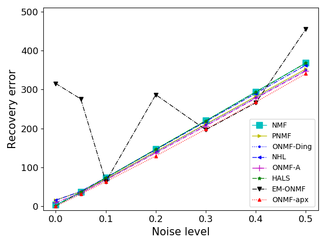
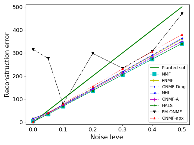
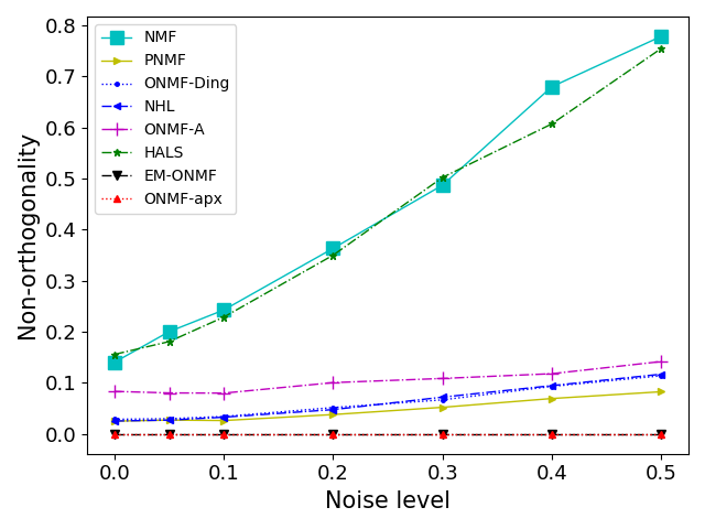
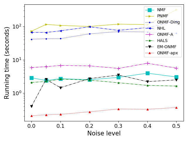
Figure 2: Results of experiment 1. From left to right, the plots in the first row show the recovery error and the reconstruction error, and the plots in the second row show the non-orthogonality and the running time. The performance of our algorithm is shown in the red line under the label ONMF-apx.

As shown in Figure 2, our algorithm ensures perfect orthogonality and gives similar approximation error as previous ones which do not guarantee orthogonality. Except for EM-ONMF, none of the other previous algorithms in this experiment output a perfectly orthogonal $W$. Our recovery error is slightly better than previous algorithms, but our reconstruction error is slightly worse. This is because the orthogonality constraint effectively regularizes our solution, making it fit the noise in the input worse but reveal the structure of the input better. It is worth noting that our algorithm achieves lower reconstruction errors than the planted solution $M_{\textup{truth}}$, and so do most other algorithms in the experiment (the reconstruction error of $M_{\textup{truth}}$ concentrates well around $1000$ times the noise level (thick green line in Figure 2) by Fact 11).

We would also like to point out that our algorithm runs significantly faster than all the other algorithms considered in this experiment. The bottom right plot of Figure 2 shows the running time on a machine with 1.4 GHz Quad-Core Intel Core i5 processor and 8 GB 2133 MHz LPDDR3 memory (note that the $y$-axis is on logarithmic scale). Our algorithm is based on the $k$-means++ subroutine, which is very efficient. The previous algorithms are based on iterative update and may take a long time to reach a local optimum.

Experiment 2

We compare our algorithm with ONMFS (Asteris et al., 2015), an algorithm that guarantees perfect orthogonality, but runs in time exponential in the squared inner dimension. ONMFS was based on two levels of exhaustive search, which is inefficient when the inner dimension is large. We thus reduce the sizes of the matrices and set $m=10,n=50,k=2$ in this experiment. Our result shows that our algorithm gives smaller error than ONMFS (Figure 3).

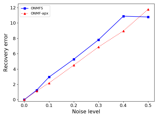
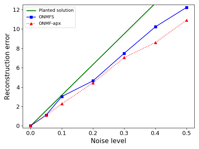
Figure 3: Results of experiment 2. From left to right, the plots show the recovery error and the reconstruction error. The non-orthogonality (not shown in figure) is identically zero for both algorithms.

Appendix A Proof of Lemma 1

Before proving Lemma 1, we first show how it gives a constant-factor approximation for bipartite correlation clustering. Given a complete bipartite graph with vertex bipartition $U\cup V$ and edges labeled $+$ or $-$, we can construct a binary matrix $M$ whose rows correspond to the vertices in $U$ and columns correspond to the vertices in $V$. An entry of $M$ is $1$ if and only if the corresponding edge is labeled $+$. The optimal solution to the correlation clustering problem also gives a binary matrix, where each cluster in the solution gives an all-ones block. Because of the block-wise structure, the matrix can be written in the form $A^{\mathrm{opt}}W^{\mathrm{opt}}$, where $A^{\mathrm{opt}},W^{\mathrm{opt}}$ give a feasible solution to the orthogonal non-negative factorization problem for $M$ with the inner-dimension being the number of clusters in the optimal solution, and the squared Frobenius error $E^{\mathrm{opt}}:=\|M-A^{\mathrm{opt}}W^{\mathrm{opt}}\|_{F}^{2}$ equals to the optimal number of disagreements for the correlation clustering problem.

By Theorem 9, we can compute an orthogonal non-negative factorization $A^{\mathrm{frac}}W^{\mathrm{frac}}$ with inner dimension $k=\min\{|U|,|V|\}$ such that $E^{\mathrm{frac}}:=\|M-A^{\mathrm{frac}}W^{\mathrm{frac}}\|_{F}^{2}\leq 15E^{\mathrm{opt}}$. Note that $E^{\mathrm{frac}}$ can be decomposed block-wise:

$$E^{\mathrm{frac}}:=E^{\mathrm{frac}}_{1}+\cdots+E^{\mathrm{frac}}_{k}+E^{\mathrm{frac}}_{*},$$

where $E^{\mathrm{frac}}_{i}$ is the sum of squared errors in block $i$, and $E^{\mathrm{frac}}_{*}$ is the sum of squared errors outside of the $k$ blocks. Applying Lemma 1 to every block, we can compute an orthogonal non-negative factorization $A^{\mathrm{bin}}W^{\mathrm{bin}}$ such that every entry of $A^{\mathrm{bin}}$ and $W^{\mathrm{bin}}$ are binary, and the sum of squared errors in each block satisfies $E^{\mathrm{bin}}_{i}\leq 8E^{\mathrm{frac}}_{i}$. We also have $E^{\mathrm{bin}}_{*}=E^{\mathrm{frac}}_{*}$ because both $A^{\mathrm{bin}}W^{\mathrm{bin}}$ and $A^{\mathrm{frac}}W^{\mathrm{frac}}$ have zeros outside the $k$ blocks. Summing up, we have

$$E^{\mathrm{bin}}:={} \|M-A^{\mathrm{bin}}W^{\mathrm{bin}}\|_{F}^{2}$$

$$={} E^{\mathrm{bin}}_{1}+\cdots+E^{\mathrm{bin}}_{k}+E^{\mathrm{bin}}_{*}$$

$$\leq{} 8\,E^{\mathrm{frac}}_{1}+\cdots+8\,E^{\mathrm{frac}}_{k}+E^{\mathrm{frac}}_{*}$$

$$\leq{} 8E^{\mathrm{frac}}$$

$$\leq{} 8\cdot 15E^{\mathrm{opt}}.$$

Thus, if we translate every block of $A^{\mathrm{bin}}W^{\mathrm{bin}}$ to a cluster of vertices, we get a $8\cdot 15=120$ approximate solution to the correlation clustering problem.

We now return to proving Lemma 1.

Proof.

Write ${\bm{w}}$ as $(w_{1},w_{2},\ldots,w_{n})^{\mathsf{T}}$ and $\hat{\bm{w}}$ as $(\hat{w}_{1},\hat{w}_{2},\ldots,\hat{w}_{n})^{\mathsf{T}}$. Let ${\bm{m}}_{i}$ denote the $i$-th column of $M$. We will construct $\hat{\bm{a}},\hat{\bm{w}}$ so that $\|{\bm{m}}_{i}-\hat{w}_{i}\hat{\bm{a}}\|_{2}^{2}\leq 8\|{\bm{m}}_{i}-w_{i}{\bm{a}}\|_{2}^{2}$ holds true for all $i$. If some $w_{i}=0$, we can always set $\hat{w}_{i}=0$. Therefore, without loss of generality, we can assume every $w_{i}$ is non-zero. Let $i^{*}\in\operatorname*{arg\,min}_{1\leq i\leq n}\|\frac{{\bm{m}}_{i}}{w_{i}}-{\bm{a}}\|_{2}^{2}$. Define $\hat{\bm{a}}={\bm{m}}_{i^{*}}$. Now we have $\forall 1\leq i\leq n$,

$$\left\|{\bm{m}}_{i}-\frac{w_{i}}{w_{i^{*}}}\hat{\bm{a}}\right\|_{2}^{2}$$

$$\leq 2\|{\bm{m}}_{i}-w_{i}{\bm{a}}\|_{2}^{2}+2\left\|\frac{w_{i}}{w_{i^{*}}}\hat{\bm{a}}-w_{i}{\bm{a}}\right\|_{2}^{2}$$ (9)

$$= 2\|{\bm{m}}_{i}-w_{i}{\bm{a}}\|_{2}^{2}+2w_{i}^{2}\left\|\frac{\hat{\bm{a}}}{w_{i^{*}}}-{\bm{a}}\right\|_{2}^{2}$$

$$\leq 2\|{\bm{m}}_{i}-w_{i}{\bm{a}}\|_{2}^{2}+2w_{i}^{2}\left\|\frac{{\bm{m}}_{i}}{w_{i}}-{\bm{a}}\right\|_{2}^{2}$$ (10)

$$= 4\|{\bm{m}}_{i}-w_{i}{\bm{a}}\|_{2}^{2}.$$ (11)

Here (9) is by Fact 4, and (10) is by the optimality of $i^{*}$ and $\hat{\bm{a}}={\bm{m}}_{i^{*}}$.

Let $S\subseteq\{1,\ldots,m\}$ be the support of $\hat{\bm{a}}={\bm{m}}_{i^{*}}$. Decompose ${\bm{m}}_{i}$ as ${\bm{m}}_{i}={\bm{m}}_{i}^{1}+{\bm{m}}_{i}^{2}$ where ${\bm{m}}_{i}^{1}$ is supported on $S$ and ${\bm{m}}_{i}^{2}$ is supported on $\bar{S}$. Let $T$ be the support of ${\bm{m}}_{i}^{1}$. Let $p\in[0,1]$ denote $\frac{|T|}{|S|}$. Define $\hat{w}_{i}=1$ if $p\geq\frac{1}{2}$ and $\hat{w}_{i}=0$ otherwise. Now we have

$$\left\|{\bm{m}}_{i}-\frac{w_{i}}{w_{i^{*}}}\hat{\bm{a}}\right\|_{2}^{2}$$

$$= \left\|{\bm{m}}_{i}^{1}-\frac{w_{i}}{w_{i^{*}}}\hat{\bm{a}}\right\|_{2}^{2}+\|{\bm{m}}_{i}^{2}\|_{2}^{2}$$

$$= |S|\left(p\left(1-\frac{w_{i}}{w_{i^{*}}}\right)^{2}+(1-p)\left(\frac{w_{i}}{w_{i^{*}}}\right)^{2}\right)+\|{\bm{m}}_{i}^{2}\|_{2}^{2}$$

$$\geq |S|p(1-p)+\|{\bm{m}}_{i}^{2}\|_{2}^{2}$$ (12)

$$\geq \frac{1}{2}|S|\min\{p,1-p\}+\|{\bm{m}}_{i}^{2}\|_{2}^{2}$$

$$= \frac{1}{2}\|{\bm{m}}_{i}^{1}-\hat{w}_{i}\hat{\bm{a}}\|_{2}^{2}+\|{\bm{m}}_{i}^{2}\|_{2}^{2}$$

$$\geq \frac{1}{2}(\|{\bm{m}}_{i}^{1}-\hat{w}_{i}\hat{\bm{a}}\|_{2}^{2}+\|{\bm{m}}_{i}^{2}\|_{2}^{2})$$

$$= \frac{1}{2}\|{\bm{m}}_{i}-\hat{w}_{i}\hat{\bm{a}}\|_{2}^{2}.$$ (13)

Here (12) is by Cauchy-Schwarz:

$$\left(p(1-t)^{2}+(1-p)t^{2}\right)((1-p)+p)\geq\left(\sqrt{p(1-p)}\cdot(1-t)+\sqrt{p(1-p)}\cdot t\right)^{2}=p(1-p).$$

Combining (11) and (13), we have $\|{\bm{m}}_{i}-\hat{w}_{i}\hat{\bm{a}}\|_{2}^{2}\leq 8\|{\bm{m}}_{i}-w_{i}{\bm{a}}\|_{2}^{2}$. Moreover, it’s clear that $\hat{\bm{a}}$ and $\hat{\bm{w}}=(\hat{w}_{1},\ldots,\hat{w}_{n})^{\mathsf{T}}$ can be computed in poly-time. ∎

Appendix B Proof of Fact 2

Proof.

The claim holds trivially when either ${\bm{x}}$ or ${\bm{y}}$ is the zero vector. Now we consider ${\bm{x}}$ being a unit vector and ${\bm{y}}$ being a non-zero vector. Let $\alpha\in[0,\pi/2]$ denote the angle between ${\bm{x}}$ and ${\bm{y}}$. Note that $\|{\bm{y}}-\theta{\bm{x}}\|_{2}$ is at least the distance from point ${\bm{y}}$ to the line defined by $\{\theta{\bm{x}}:\theta\in\mathbb{R}\}$, so we have $\|{\bm{y}}-\theta{\bm{x}}\|_{2}\geq\|{\bm{y}}\|_{2}\sin\alpha$. On the other hand, $\|\bar{\bm{y}}-{\bm{x}}\|_{2}^{2}=2-2\langle\bar{\bm{y}},{\bm{x}}\rangle=2-2\cos\alpha$. Therefore, the lemma reduces to

$$\sin^{2}\alpha\geq 1-\cos\alpha,$$

which is obviously true because $1=\sin^{2}\alpha+\cos^{2}\alpha$ and $\cos\alpha\geq\cos^{2}\alpha$. ∎

Appendix C Proof of Theorem 3

Proof.

It is clear that $(A,W)$ is a feasible solution, and the computation we need besides the weighted $k$-means subroutine can be done in time linear in the number of entries in $M$, which justifies the claimed running time. We now prove that it achieves an objective at most $2r$ times that achieved by the optimal solution $(A^{\mathrm{opt}},W^{\mathrm{opt}})$. We can assume WLOG that each column ${\bm{a}}_{s}^{\mathrm{opt}}$ of $A^{\mathrm{opt}}$ is either a unit vector or the zero vector because we can scale up a column of $A$ and scale down the corresponding row of $W$ by the same factor without changing the product $AW$. Since the rows of $W^{\mathrm{opt}}$ are non-negative and orthogonal, they have disjoint supports, so there exists $\phi^{\prime}:\{1,\ldots,n\}\rightarrow\{1,\ldots,k\}$ and $\theta_{1}^{\prime},\ldots,\theta_{n}^{\prime}\in\mathbb{R}_{\geq 0}$ such that for all $i=1,\ldots,n$, the $i$-th column of $W^{\mathrm{opt}}$ is $\theta_{i}^{\prime}{\bm{e}}_{\phi^{\prime}(i)}$.

Now we have

$$\|M-A^{\mathrm{opt}}W^{\mathrm{opt}}\|_{F}^{2}$$

$$= \sum_{i=1}^{n}\|{\bm{m}}_{i}-\theta_{i}^{\prime}{\bm{a}}_{\phi^{\prime}(i)}\|_{2}^{2}$$

$$\geq \frac{1}{2}\sum_{i=1}^{n}\|{\bm{m}}_{i}\|_{2}^{2}\|\bar{\bm{m}}_{i}-{\bm{a}}_{\phi^{\prime}(i)}\|_{2}^{2}$$ (14)

$$\geq \frac{1}{2r}\sum_{i=1}^{n}\|{\bm{m}}_{i}\|_{2}^{2}\|\bar{\bm{m}}_{i}-{\bm{c}}_{\phi(i)}\|_{2}^{2}$$ (15)

$$= \frac{1}{2r}\sum_{i=1}^{n}\|{\bm{m}}_{i}-\|{\bm{m}}_{i}\|_{2}{\bm{c}}_{\phi(i)}\|_{2}^{2}$$

$$\geq \frac{1}{2r}\sum_{i=1}^{n}\|{\bm{m}}_{i}-\theta_{i}{\bm{c}}_{\phi(i)}\|_{2}^{2}$$ (16)

$$= \frac{1}{2r}\|M-AW\|_{F}^{2}.$$

Here, (14) is by Fact 2, (15) is because $({\bm{c}},\phi)$ is an $r$-approximate solution to (1), and (16) is because $\theta_{i}\in\operatorname*{arg\,min}_{\theta}\|{\bm{m}}_{i}-\theta{\bm{c}}_{\phi(i)}\|_{2}^{2}$. ∎

Appendix D Proof of Lemma 10

Proof.

First, we show the following inequality for $q_{j}^{\prime}$ instead of $q_{j}$:

$$\sum_{j=1}^{k}q^{\prime}_{j}\|{\bm{c}}_{j}-{\bm{a}}_{\sigma(j)}\|_{2}^{2}\leq 8\sum_{j=1}^{k}q^{\prime}_{j}\|{\bm{c}}_{j}-{\bm{z}}_{\sigma^{\prime}(j)}\|_{2}^{2}.$$ (17)

We start by constructing an alternative feasible solution to (2): ${\bm{a}}_{1}^{\prime},\ldots,{\bm{a}}_{k}^{\prime}\in\{{\bm{0}},{\bm{z}}_{1},\ldots,{\bm{z}}_{k_{1}}\}$. For any ${\bm{c}}_{j}$ with $q^{\prime}_{j}>0$, we say $j$ is “matched” if $\angle({\bm{c}}_{j},{\bm{z}}_{\sigma^{\prime}(j)})<\frac{\pi}{6}$. Note that if $\sigma(j_{1})=\sigma(j_{2})$ and they are both “matched”, then we must have ${\bm{z}}_{\sigma^{\prime}(j_{1})}={\bm{z}}_{\sigma^{\prime}(j_{2})}$, because otherwise $\frac{\pi}{2}=\angle({\bm{z}}_{\sigma^{\prime}(j_{1})},{\bm{z}}_{\sigma^{\prime}(j_{2})})\leq\angle({\bm{c}}_{j_{1}},{\bm{z}}_{\sigma^{\prime}(j_{1})})+\angle({\bm{c}}_{j_{2}},{\bm{z}}_{\sigma^{\prime}(j_{2})})+\angle({\bm{c}}_{j_{1}},{\bm{c}}_{j_{2}})<\frac{\pi}{6}+\frac{\pi}{6}+\frac{\pi}{6}$, a contradiction. Also, if $\sigma(j_{1})\neq\sigma(j_{2})$ and they are both “matched”, then we must have ${\bm{z}}_{\sigma^{\prime}(j_{1})}\neq{\bm{z}}_{\sigma^{\prime}(j_{2})}$, because otherwise $\frac{\pi}{3}<\angle({\bm{c}}_{j_{1}},{\bm{c}}_{j_{2}})\leq\angle({\bm{c}}_{j_{1}},{\bm{z}}_{\sigma^{\prime}(j_{1})})+\angle({\bm{c}}_{j_{2}},{\bm{z}}_{\sigma^{\prime}(j_{2})})<\frac{\pi}{6}+\frac{\pi}{6}$, a contradiction again. Therefore, we can uniquely define ${\bm{a}}^{\prime}_{s}$ to be ${\bm{z}}_{\sigma^{\prime}(j)}$ whenever there exists a “matched” $j$ in $\sigma^{-1}(s)$, and we know different $s$ must correspond to different ${\bm{a}}^{\prime}_{s}$. When such a “matched” $j$ in $\sigma^{-1}(s)$ does not exist, we simply define ${\bm{a}}^{\prime}_{s}={\bm{0}}$. Now ${\bm{a}}_{1}^{\prime},\ldots,{\bm{a}}_{k}^{\prime}$ are orthogonal to each other, so by the optimality of ${\bm{a}}_{1},\ldots,{\bm{a}}_{k}$ in solving (2), we have

$$\sum_{j=1}^{k}q^{\prime}_{j}\|{\bm{c}}_{j}-{\bm{a}}_{\sigma(j)}\|_{2}^{2}\leq\sum_{j=1}^{k}q^{\prime}_{j}\|{\bm{c}}_{j}-{\bm{a}}^{\prime}_{\sigma(j)}\|_{2}^{2}.$$

In order to prove (17), we now only need to show that for every $j$ with $q_{j}^{\prime}>0$, $\|{\bm{c}}_{j}-{\bm{a}}^{\prime}_{\sigma(j)}\|_{2}^{2}\leq 8\|{\bm{c}}_{j}-{\bm{z}}_{\sigma^{\prime}(j)}\|_{2}^{2}$. This is obviously true when $j$ is “matched” since ${\bm{a}}^{\prime}_{\sigma(j)}={\bm{z}}_{\sigma^{\prime}(j)}$. When $j$ is not “matched”, we have $\angle({\bm{c}}_{j},{\bm{z}}_{\sigma^{\prime}(j)})\geq\frac{\pi}{6}$, so $\|{\bm{c}}_{j}-{\bm{z}}_{\sigma^{\prime}(j)}\|_{2}^{2}\geq\sin^{2}\frac{\pi}{6}=1/4$, while $\|{\bm{c}}_{j}-{\bm{a}}^{\prime}_{\sigma(j)}\|_{2}^{2}\leq\|{\bm{c}}_{j}\|_{2}^{2}+\|{\bm{a}}^{\prime}_{\sigma(j)}\|_{2}^{2}\leq 2$ by Fact 5. Therefore, $\|{\bm{c}}_{j}-{\bm{a}}^{\prime}_{\sigma(j)}\|_{2}^{2}\leq 8\|{\bm{c}}_{j}-{\bm{z}}_{\sigma^{\prime}(j)}\|_{2}^{2}$ is also true when $j$ is not “matched”.

Now we prove

$$\sum_{j=1}^{k}(q_{j}-q^{\prime}_{j})\|{\bm{c}}_{j}-{\bm{a}}_{\sigma(j)}\|_{2}^{2}\leq\frac{2}{\sin^{2}(\pi/12)}\sum_{j=1}^{k}(q_{j}-q^{\prime}_{j})\|{\bm{c}}_{j}-{\bm{z}}_{\sigma^{\prime}(j)}\|_{2}^{2}.$$ (18)

We can decompose $q_{j}-q^{\prime}_{j}$ by the iterations of the weight reduction step. Let $\mathbb{I}_{t}(j)$ denote the indicator for ${\bm{c}}_{j}$ being chosen in the $t$-th iteration of weight reduction, and let $\Delta_{t}\geq 0$ denote the decrease in weight in the $t$-th iteration. We have $q_{j}-q^{\prime}_{j}=\sum_{t}\mathbb{I}_{t}(j)\Delta_{t}$. Swapping sums, (18) is equivalent to

$$\sum_{t}\Delta_{t}\sum_{j=1}^{k}\mathbb{I}_{t}(j)\|{\bm{c}}_{j}-{\bm{a}}_{\sigma(j)}\|_{2}^{2}\leq\frac{2}{\sin^{2}(\pi/12)}\sum_{t}\Delta_{t}\sum_{j=1}^{k}\mathbb{I}_{t}(j)\|{\bm{c}}_{j}-{\bm{z}}_{\sigma^{\prime}(j)}\|_{2}^{2}.$$

Note that for a fixed $t$, $\mathbb{I}_{t}(j)=1$ if and only if $j\in\{j_{1},j_{2}\}$, where pair $(j_{1},j_{2})$ is selected in the $t$-th iteration of the weight reduction step. Thus, to prove (18), it suffices to prove that whenever $(j_{1},j_{2})$ is selected in the weight reduction step, we have $\|{\bm{c}}_{j_{1}}-{\bm{a}}_{\sigma(j_{1})}\|_{2}^{2}+\|{\bm{c}}_{j_{2}}-{\bm{a}}_{\sigma(j_{2})}\|_{2}^{2}\leq\frac{2}{\sin^{2}(\pi/12)}\left(\|{\bm{c}}_{j_{1}}-{\bm{z}}_{\sigma^{\prime}(j_{1})}\|_{2}^{2}+\|{\bm{c}}_{j_{2}}-{\bm{z}}_{\sigma^{\prime}(j_{2})}\|_{2}^{2}\right)$. Define $\alpha_{1}:=\angle({\bm{c}}_{j_{1}},{\bm{z}}_{\sigma^{\prime}(j_{1})})$ and $\alpha_{2}:=\angle({\bm{c}}_{j_{2}},{\bm{z}}_{\sigma^{\prime}(j_{2})})$. Since $\angle({\bm{c}}_{j_{1}},{\bm{c}}_{j_{2}})\in[\pi/6,\pi/3]$, we always have $\alpha_{1}+\alpha_{2}\geq\pi/6$, whether or not $\sigma^{\prime}(j_{1})=\sigma^{\prime}(j_{2})$. Therefore, we have $\|{\bm{c}}_{j_{1}}-{\bm{z}}_{\sigma^{\prime}(j_{1})}\|_{2}^{2}+\|{\bm{c}}_{j_{2}}-{\bm{z}}_{\sigma^{\prime}(j_{2})}\|_{2}^{2}\geq\sin^{2}\alpha_{1}+\sin^{2}\alpha_{2}\geq 2\sin^{2}\frac{\pi}{12}$ by the convexity and monotonicity of $\sin^{2}x$ over $[0,\pi/2]$. On the other hand, $\|{\bm{c}}_{j_{1}}-{\bm{a}}_{\sigma(j_{1})}\|_{2}^{2}+\|{\bm{c}}_{j_{2}}-{\bm{a}}_{\sigma(j_{2})}\|_{2}^{2}\leq\|{\bm{c}}_{j_{1}}\|_{2}^{2}+\|{\bm{a}}_{\sigma(j_{1})}\|_{2}^{2}+\|{\bm{c}}_{j_{2}}\|_{2}^{2}+\|{\bm{a}}_{\sigma(j_{2})}\|_{2}^{2}\leq 4$ by Fact 5. This concludes the proof of $\|{\bm{c}}_{j_{1}}-{\bm{a}}_{\sigma(j_{1})}\|_{2}^{2}+\|{\bm{c}}_{j_{2}}-{\bm{a}}_{\sigma(j_{2})}\|_{2}^{2}\leq\frac{2}{\sin^{2}(\pi/12)}\left(\|{\bm{c}}_{j_{1}}-{\bm{z}}_{\sigma^{\prime}(j_{1})}\|_{2}^{2}+\|{\bm{c}}_{j_{2}}-{\bm{z}}_{\sigma^{\prime}(j_{2})}\|_{2}^{2}\right)$.

Combining (17) with (18) proves the Lemma. ∎

Appendix E Proof of Theorem 9

Proof.

By symmetry ($\|M-AW\|_{F}^{2}=\|M^{\mathsf{T}}-W^{\mathsf{T}}A^{\mathsf{T}}\|_{F}^{2}$), we can assume WLOG that $k\geq n$. In this special case, the first step of the algorithm, solving weighted $k$-means, becomes trivial. We can simply choose $\phi(i)=i,{\bm{c}}_{i}=\bar{\bm{m}}_{i}$ and $q_{i}=\ell_{i}$. The second and the third steps remain the same.

To analyze the approximation ratio, we first write $\|M-AW\|_{F}^{2}$ as

$$\|M-AW\|_{F}^{2}=\sum_{i=1}^{n}\|{\bm{m}}_{i}-\theta_{i}{\bm{a}}_{\sigma(i)}\|_{2}^{2}=\sum_{i=1}^{n}q_{i}\|\bar{\bm{m}}_{i}-\bar{\theta}_{i}{\bm{a}}_{\sigma(i)}\|_{2}^{2},$$ (19)

where $\bar{\theta}_{i}=\left\{\begin{array}[]{ll}\frac{\langle\bar{\bm{m}}_{i},{\bm{a}}_{\sigma(i)}\rangle}{\|{\bm{a}}_{\sigma(i)}\|_{2}^{2}},&\textup{if }{\bm{a}}_{\sigma(i)}\neq{\bm{0}}\\ 0,&\textup{if }{\bm{a}}_{\sigma(i)}={\bm{0}}\end{array}\right.$.

Similarly to Lemma 10, we have the following lemma (proved in Appendix F):

Lemma 12.

Let ${\bm{z}}_{1},\ldots,{\bm{z}}_{k_{1}}\in\mathbb{R}^{m}_{\geq 0}$ be non-negative unit vectors that are orthogonal to each other. For any $\sigma^{\prime}:\{1,\ldots,n\}\rightarrow\{1,\ldots,k^{\prime}\}$, we have

$$\sum_{i=1}^{n}q_{i}\|\bar{\bm{m}}_{i}-\bar{\theta}_{i}{\bm{a}}_{\sigma(i)}\|_{2}^{2}\leq\frac{1}{\sin^{2}(\pi/12)}\sum_{i=1}^{n}q_{i}\|\bar{\bm{m}}_{i}-\langle\bar{\bm{m}}_{i},{\bm{z}}_{\sigma^{\prime}(i)}\rangle{\bm{z}}_{\sigma^{\prime}(i)}\|_{2}^{2}.$$ (20)

Suppose the optimal solution is $(A^{\mathrm{opt}},W^{\mathrm{opt}})$. Again, we remove the columns of $A^{\mathrm{opt}}$ filled with the zero vector and also remove the corresponding rows in $W^{\mathrm{opt}}$. Suppose the sizes of $A^{\mathrm{opt}}$ and $W^{\mathrm{opt}}$ now change to $m\times k_{1}$ and $k_{1}\times n$. We assume WLOG that every column ${\bm{a}}^{\mathrm{opt}}_{s}$ of $A^{\mathrm{opt}}$ is a unit vector. Suppose the $i$-th column of $W^{\mathrm{opt}}$ is $\theta_{i}^{\prime}{\bm{e}}_{\phi^{\prime}(i)}$. We have

$$\|M-A^{\mathrm{opt}}W^{\mathrm{opt}}\|_{F}^{2}= \sum_{i=1}^{n}\|{\bm{m}}_{i}-\theta_{i}^{\prime}{\bm{a}}^{\mathrm{opt}}_{\phi^{\prime}(i)}\|_{2}^{2}$$

$$\geq \sum_{i=1}^{n}\|{\bm{m}}_{i}-\langle{\bm{m}}_{i},{\bm{a}}^{\mathrm{opt}}_{\phi^{\prime}(i)}\rangle{\bm{a}}^{\mathrm{opt}}_{\phi^{\prime}(i)}\|_{2}^{2}$$

$$= \sum_{i=1}^{n}q_{i}\|\bar{\bm{m}}_{i}-\langle\bar{\bm{m}}_{i},{\bm{a}}^{\mathrm{opt}}_{\phi^{\prime}(i)}\rangle{\bm{a}}^{\mathrm{opt}}_{\phi^{\prime}(i)}\|_{2}^{2}.$$ (21)

Setting ${\bm{z}}_{\sigma^{\prime}(i)}$ in (20) to be ${\bm{a}}^{\mathrm{opt}}_{\phi^{\prime}(i)}$ and combining it with (19) and (21), we have $\|M-AW\|_{F}^{2}\leq\frac{1}{\sin^{2}(\pi/12)}\|M-A^{\mathrm{opt}}W^{\mathrm{opt}}\|_{F}^{2}$. ∎

Appendix F Proof of Lemma 12

Proof.

The proof is very similar to the proof of Lemma 10. First, we show the following inequality for $q_{i}^{\prime}$ instead of $q_{i}$:

$$\sum_{i=1}^{n}q^{\prime}_{i}\|\bar{\bm{m}}_{i}-\bar{\theta}_{i}{\bm{a}}_{\sigma(i)}\|_{2}^{2}\leq 8\sum_{i=1}^{n}q^{\prime}_{i}\|\bar{\bm{m}}_{i}-\langle\bar{\bm{m}}_{i},{\bm{z}}_{\sigma^{\prime}(i)}\rangle{\bm{z}}_{\sigma^{\prime}(i)}\|_{2}^{2}.$$ (22)

Note that $\bar{\theta}_{i}\in\operatorname*{arg\,min}_{\theta\geq 0}\|\bar{\bm{m}}_{i}-\theta{\bm{a}}_{\sigma(i)}\|_{2}^{2}$. Therefore,

$$\sum_{i=1}^{n}q^{\prime}_{i}\|\bar{\bm{m}}_{i}-\bar{\theta}_{i}{\bm{a}}_{\sigma(i)}\|_{2}^{2}\leq\sum_{i=1}^{n}q^{\prime}_{i}\|\bar{\bm{m}}_{i}-{\bm{a}}_{\sigma(i)}\|_{2}^{2}.$$

We now construct an alternative feasible solution to (2): ${\bm{a}}_{1}^{\prime},\ldots,{\bm{a}}_{k}^{\prime}\in\{{\bm{0}},{\bm{z}}_{1},\ldots,{\bm{z}}_{k_{1}}\}$. For any $\bar{\bm{m}}_{i}$ with $q^{\prime}_{i}>0$, we say $i$ is “matched” if $\angle(\bar{\bm{m}}_{i},{\bm{z}}_{\sigma^{\prime}(i)})<\frac{\pi}{6}$. Note that if $\sigma(i_{1})=\sigma(i_{2})$ and they are both “matched”, then we must have ${\bm{z}}_{\sigma^{\prime}(i_{1})}={\bm{z}}_{\sigma^{\prime}(i_{2})}$, because otherwise $\frac{\pi}{2}=\angle({\bm{z}}_{\sigma^{\prime}(i_{1})},{\bm{z}}_{\sigma^{\prime}(i_{2})})\leq\angle(\bar{\bm{m}}_{i_{1}},{\bm{z}}_{\sigma^{\prime}(i_{1})})+\angle(\bar{\bm{m}}_{i_{2}},{\bm{z}}_{\sigma^{\prime}(i_{2})})+\angle(\bar{\bm{m}}_{i_{1}},\bar{\bm{m}}_{i_{2}})<\frac{\pi}{6}+\frac{\pi}{6}+\frac{\pi}{6}$, a contradiction. Also, if $\sigma(i_{1})\neq\sigma(i_{2})$ and they are both “matched”, then we must have ${\bm{z}}_{\sigma^{\prime}(i_{1})}\neq{\bm{z}}_{\sigma^{\prime}(i_{2})}$, because otherwise $\frac{\pi}{3}<\angle(\bar{\bm{m}}_{i_{1}},\bar{\bm{m}}_{i_{2}})\leq\angle(\bar{\bm{m}}_{i_{1}},{\bm{z}}_{\sigma^{\prime}(i_{1})})+\angle(\bar{\bm{m}}_{i_{2}},{\bm{z}}_{\sigma^{\prime}(i_{2})})<\frac{\pi}{6}+\frac{\pi}{6}$, a contradiction again. Therefore, we can uniquely define ${\bm{a}}^{\prime}_{s}$ to be ${\bm{z}}_{\sigma^{\prime}(i)}$ whenever there exists a “matched” $i$ in $\sigma^{-1}(s)$, and we know different $s$ must correspond to different ${\bm{a}}^{\prime}_{s}$. When such a “matched” $i$ in $\sigma^{-1}(s)$ does not exist, we simply define ${\bm{a}}^{\prime}_{s}={\bm{0}}$. Now ${\bm{a}}_{1}^{\prime},\ldots,{\bm{a}}_{k}^{\prime}$ are orthogonal to each other, so by the optimality of ${\bm{a}}_{1},\ldots,{\bm{a}}_{k}$ in solving (2), we have

$$\sum_{i=1}^{n}q^{\prime}_{i}\|\bar{\bm{m}}_{i}-{\bm{a}}_{\sigma(i)}\|_{2}^{2}\leq\sum_{i=1}^{n}q^{\prime}_{i}\|\bar{\bm{m}}_{i}-{\bm{a}}^{\prime}_{\sigma(i)}\|_{2}^{2}\leq 2\sum_{i=1}^{n}q^{\prime}_{i}\|\bar{\bm{m}}_{i}-\langle\bar{\bm{m}}_{i},{\bm{a}}^{\prime}_{\sigma(i)}\rangle{\bm{a}}^{\prime}_{\sigma(i)}\|_{2}^{2},$$

where the second inequality is by Fact 2 and the fact that ${\bm{a}}^{\prime}_{\sigma(i)}$ is either the zero vector or a unit vector.

In order to prove (22), we now only need to show that for every $i$ with $q_{i}^{\prime}>0$,

$$\|\bar{\bm{m}}_{i}-\langle\bar{\bm{m}}_{i},{\bm{a}}^{\prime}_{\sigma(i)}\rangle{\bm{a}}^{\prime}_{\sigma(i)}\|_{2}^{2}\leq 4\|\bar{\bm{m}}_{i}-\langle\bar{\bm{m}}_{i},{\bm{z}}_{\sigma^{\prime}(i)}\rangle{\bm{z}}_{\sigma^{\prime}(i)}\|_{2}^{2}.$$ (23)

This is obviously true when $i$ is “matched” since ${\bm{a}}^{\prime}_{\sigma(i)}={\bm{z}}_{\sigma^{\prime}(i)}$. When $i$ is not “matched”, we have $\angle(\bar{\bm{m}}_{i},{\bm{z}}_{\sigma^{\prime}(i)})\geq\frac{\pi}{6}$. Since $q_{i}\geq q_{i}^{\prime}>0$, we know $\bar{\bm{m}}_{i}$ is a unit vector rather than the zero vector, so $\|\bar{\bm{m}}_{i}-\langle\bar{\bm{m}}_{i},{\bm{z}}_{\sigma^{\prime}(i)}\rangle{\bm{z}}_{\sigma^{\prime}(i)}\|_{2}^{2}\geq\sin^{2}\frac{\pi}{6}=1/4$, while $\|\bar{\bm{m}}_{i}-\langle\bar{\bm{m}}_{i},{\bm{a}}^{\prime}_{\sigma(i)}\rangle{\bm{a}}^{\prime}_{\sigma(i)}\|_{2}^{2}=\|\bar{\bm{m}}_{i}\|_{2}^{2}-\langle\bar{\bm{m}}_{i},{\bm{a}}^{\prime}_{\sigma(i)}\rangle^{2}\leq 1$. Therefore, (23) is also true when $j$ is not “matched”.

Now we prove

$$\sum_{i=1}^{n}(q_{i}-q^{\prime}_{i})\|\bar{\bm{m}}_{i}-\bar{\theta}_{i}{\bm{a}}_{\sigma(i)}\|_{2}^{2}\leq\frac{1}{\sin^{2}(\pi/12)}\sum_{i=1}^{n}(q_{i}-q^{\prime}_{i})\|\bar{\bm{m}}_{i}-\langle\bar{\bm{m}}_{i},{\bm{z}}_{\sigma^{\prime}(i)}\rangle{\bm{z}}_{\sigma^{\prime}(i)}\|_{2}^{2}.$$ (24)

Similarly to how we proved (18), it suffices to prove that whenever $(i_{1},i_{2})$ is selected in the weight reduction step, we have

$$\|\bar{\bm{m}}_{i_{1}}-\bar{\theta}_{i_{1}}{\bm{a}}_{\sigma(i_{1})}\|_{2}^{2}+\|\bar{\bm{m}}_{i_{2}}-\bar{\theta}_{i_{2}}{\bm{a}}_{\sigma(i_{2})}\|_{2}^{2}$$

$$\leq \frac{1}{\sin^{2}(\pi/12)}\left(\|\bar{\bm{m}}_{i_{1}}-\langle\bar{\bm{m}}_{i_{1}},{\bm{z}}_{\sigma^{\prime}(i_{1})}\rangle{\bm{z}}_{\sigma^{\prime}(i_{1})}\|_{2}^{2}+\|\bar{\bm{m}}_{i_{2}}-\langle\bar{\bm{m}}_{i_{2}},{\bm{z}}_{\sigma^{\prime}(i_{2})}\rangle{\bm{z}}_{\sigma^{\prime}(i_{2})}\|_{2}^{2}\right).$$ (25)

Note that here $\bar{\bm{m}}_{i_{1}}$ and $\bar{\bm{m}}_{i_{2}}$ are both unit vectors because otherwise they would have zero weights ($q_{i_{1}}=q_{i_{1}}^{\prime}=0$ or $q_{i_{2}}=q_{i_{2}}^{\prime}=0$) and wouldn’t be selected in the weight reduction step.

Define $\alpha_{1}:=\angle(\bar{\bm{m}}_{i_{1}},{\bm{z}}_{\sigma^{\prime}(i_{1})})$ and $\alpha_{2}:=\angle(\bar{\bm{m}}_{i_{2}},{\bm{z}}_{\sigma^{\prime}(i_{2})})$. Since $\angle(\bar{\bm{m}}_{i_{1}},\bar{\bm{m}}_{i_{2}})\in[\pi/6,\pi/3]$, we always have $\alpha_{1}+\alpha_{2}\geq\pi/6$, whether or not $\sigma^{\prime}(i_{1})=\sigma^{\prime}(i_{2})$. Therefore, we have

$$\left(\|\bar{\bm{m}}_{i_{1}}-\langle\bar{\bm{m}}_{i_{1}},{\bm{z}}_{\sigma^{\prime}(i_{1})}\rangle{\bm{z}}_{\sigma^{\prime}(i_{1})}\|_{2}^{2}+\|\bar{\bm{m}}_{i_{2}}-\langle\bar{\bm{m}}_{i_{2}},{\bm{z}}_{\sigma^{\prime}(i_{2})}\rangle{\bm{z}}_{\sigma^{\prime}(i_{2})}\|_{2}^{2}\right) \geq\sin^{2}\alpha_{1}+\sin^{2}\alpha_{2}$$

$$\geq 2\sin^{2}\frac{\pi}{12}$$

by the convexity and monotonicity of $\sin^{2}x$ over $[0,\pi/2]$. On the other hand, since $\bar{\theta}_{i}\in\operatorname*{arg\,min}_{\theta\geq 0}\|\bar{\bm{m}}_{i}-\theta{\bm{a}}_{\sigma(i)}\|_{2}^{2}$, we know $\|\bar{\bm{m}}_{i}-\bar{\theta}_{i}{\bm{a}}_{\sigma(i)}\|_{2}^{2}\leq\|\bar{\bm{m}}_{i}\|_{2}^{2}$, so

$$\|\bar{\bm{m}}_{i_{1}}-\bar{\theta}_{i_{1}}{\bm{a}}_{\sigma(i_{1})}\|_{2}^{2}+\|\bar{\bm{m}}_{i_{2}}-\bar{\theta}_{i_{2}}{\bm{a}}_{\sigma(i_{2})}\|_{2}^{2}$$

$$\leq \|\bar{\bm{m}}_{i_{1}}\|_{2}^{2}+\|\bar{\bm{m}}_{i_{2}}\|_{2}^{2}$$

$$= 2.$$

This concludes the proof of (25).

Combining (22) with (24) proves the Lemma. ∎

Appendix G Additional Experiments

G.1 Experiments on Real-world Data

We run our single-factor orthogonality algorithm on real-world datasets from Dua and Graff (2017). Following the setting in Asteris et al. (2015), we choose $k=6$ and use the relative squared Frobenius error (RSFE) to measure the performance of our algorithm. Suppose $M$ is the data matrix and $A,W$ are the output of the algorithm, RSFE is defined as $\|M-AW\|_{F}^{2}/\|M\|_{F}^{2}$. Note that the orthogonality constraint is posed on the left factor $A$, so we need to first transpose the data matrix before running our algorithm in Section 3. Our algorithm achieves similar RSFE compared to the best previous algorithm recorded in Table 2 of Asteris et al. (2015) on each dataset, and achieves slightly smaller (better) RSFE on datasets Arcence Train and Mfeat Pix.

Dataset	RSFE of Our Algorithm	Smallest RSFE recorded in Asteris et al. (2015)
Amzn Com. Rev	$0.0467$	0.0462
Arcence Train	$\mathbf{0.0760}$	0.0788
Mfeat Pix	$\mathbf{0.2382}$	0.2447
Pems Train	0.1279	0.1278
BoW:KOS	0.7685	0.7609
BoW:NIPS	0.7386	0.7252

Table 1: Experimental results on real-world data in the single-factor orthogonality setting.

G.2 Experiments in the Double-factor Orthogonality Setting

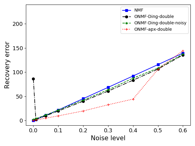
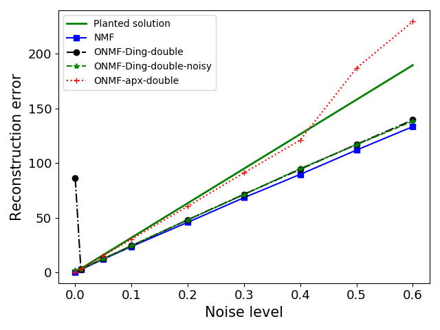
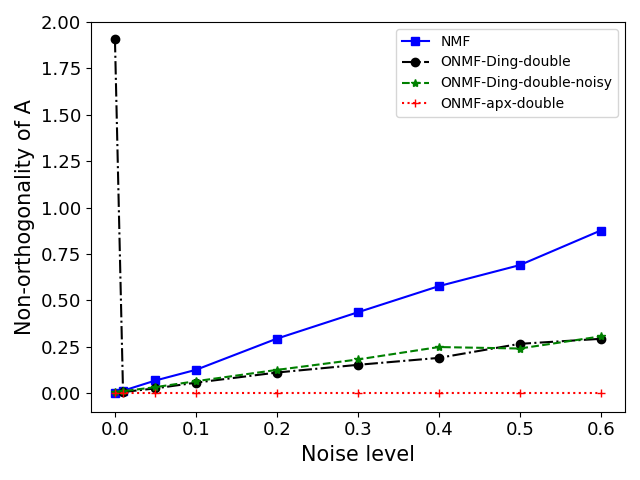
Figure 4: Experimental results in the double-factor orthogonality setting.

We extend our experiments in Section 5 to the double-factor orthogonality setting, where we generate $A_{\textup{truth}}$ with orthogonal columns and $W_{\textup{truth}}$ with orthogonal rows. The only previous algorithm we know that handles the double-factor orthogonality is ONMF-Ding-double (Ding et al., 2006), which factorizes the input matrix $M\in\mathbb{R}^{m\times n}$ as the product of three non-negative matrices $M\approx ASW$ where $A\in\mathbb{R}^{m\times k},S\in\mathbb{R}^{k\times k},W\in\mathbb{R}^{k\times n}$, with the aim of making $A$ and $W$ satisfy the orthogonality constraint approximately. We compare our algorithm with ONMF-Ding-double together with the NMF algorithm (Lee and Seung, 2001) that does not aim for orthogonality. We keep other settings in Section 5 unchanged while choosing $m=100,n=500,k=5$ so that ONMF-Ding-double can converge in a short time. While we run most algorithms 7 times and record the median results in Figure 4, ONMF-Ding-double (resp. ONMF-Ding-double-noisy) is only run once at noise level 0.01 (resp. 0.00 and 0.01) because it took too long to finish. As shown in Figure 4, our algorithm (ONMF-apx-double) is able to ensure perfect orthogonality for both factors and achieve better recovery error when the noise level is below 0.5. We note that most of the reconstruction errors of the algorithms are below the reconstruction error of the planted solution $M_{\textup{truth}}$, which concentrates well around $10^{2.5}\approx 316$ times the noise level (thick green line in Figure 4) by Fact 11. We also observe that ONMF-Ding-double takes more and more iterations to reach a solution with a reasonable approximation error as the noise level decreases towards zero, and it gets stuck at a suboptimal solution when the noise level is zero. (Adding additional iid noise from the exponential distribution with mean $0.01$ to the input alleviates this issue, but that also slightly inflates the recovery error as shown by the green lines corresponding to ONMF-Ding-double-noisy in Figure 4.)

G.3 Experiments for Different Inner Dimensions

In experiment 1 (Section 5), we fixed $k=10$ and studied how the performances of the algorithms vary with noise levels in the single-factor orthogonality setting. Now we fix the noise level to be $0.5$ and study the effect of different choices of the inner dimension $k$. We keep all other settings unchanged and record the results in Figure 5. As in experiment 1, our algorithm (ONMF-apx) achieves perfect orthogonality with a significant improvement in the running time, and has smaller recovery errors than most previous algorithms. The experiment shows a common trend that the recovery (resp. reconstruction) error increases (resp. decreases) with the inner dimension $k$, although the amount of such change in the error is insignificant (note that the $y$-axes of the plots in the first row of Figure 5 do not start from zero). Of all algorithms studied in the experiment, the errors of our algorithm change the least with the inner dimension.

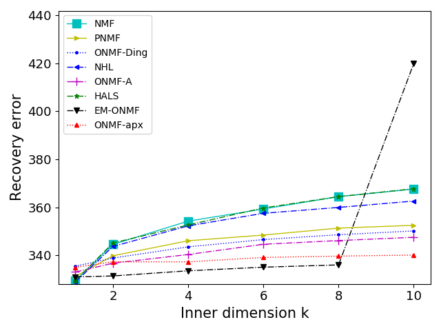
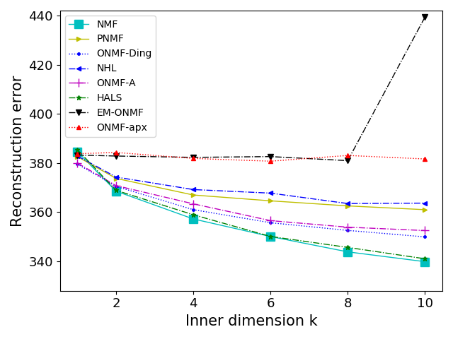
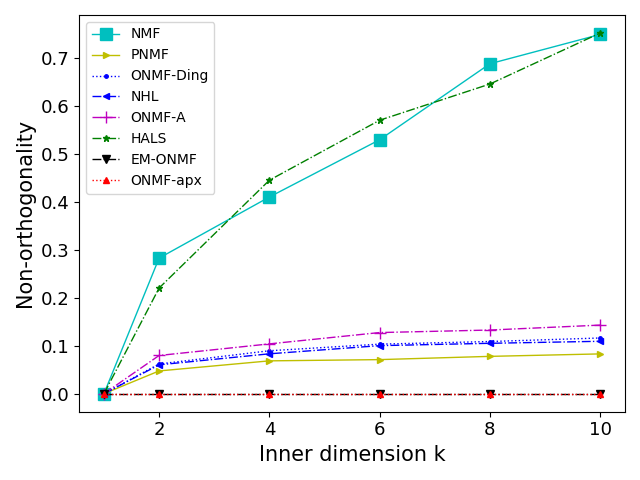
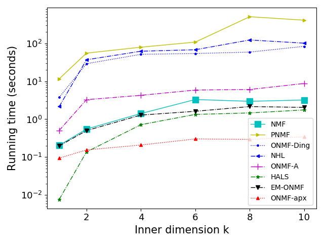
Figure 5: Experimental results with different inner dimensions $k$ in the single-factor orthogonality setting.

References

- Ahmadian et al. (2017) Sara Ahmadian, Ashkan Norouzi-Fard, Ola Svensson, and Justin Ward. Better guarantees for k-means and Euclidean k-median by primal-dual algorithms. In 2017 IEEE 58th Annual Symposium on Foundations of Computer Science (FOCS), pages 61–72. IEEE, 2017.
- Ailon et al. (2008) Nir Ailon, Moses Charikar, and Alantha Newman. Aggregating inconsistent information: ranking and clustering. Journal of the ACM (JACM), 55(5):1–27, 2008.
- Alaudah et al. (2017) YK Alaudah, Haibin Di, and Ghassan AlRegib. Weakly supervised seismic structure labeling via orthogonal non-negative matrix factorization. In 79th EAGE Conference and Exhibition 2017, volume 2017, pages 1–5. European Association of Geoscientists & Engineers, 2017.
- Alter et al. (2000) Orly Alter, Patrick O Brown, and David Botstein. Singular value decomposition for genome-wide expression data processing and modeling. Proceedings of the National Academy of Sciences, 97(18):10101–10106, 2000.
- Arora et al. (2016) Sanjeev Arora, Rong Ge, Ravi Kannan, and Ankur Moitra. Computing a nonnegative matrix factorization—provably. SIAM Journal on Computing, 45(4):1582–1611, 2016.
- Asteris et al. (2015) Megasthenis Asteris, Dimitris Papailiopoulos, and Alexandros G Dimakis. Orthogonal NMF through subspace exploration. In Advances in Neural Information Processing Systems, pages 343–351, 2015.
- Bansal et al. (2004) Nikhil Bansal, Avrim Blum, and Shuchi Chawla. Correlation clustering. Machine learning, 56(1-3):89–113, 2004.
- Brunet et al. (2004) Jean-Philippe Brunet, Pablo Tamayo, Todd R Golub, and Jill P Mesirov. Metagenes and molecular pattern discovery using matrix factorization. Proceedings of the national academy of sciences, 101(12):4164–4169, 2004.
- Chawla et al. (2015) Shuchi Chawla, Konstantin Makarychev, Tselil Schramm, and Grigory Yaroslavtsev. Near optimal LP rounding algorithm for correlation clustering on complete and complete k-partite graphs. In Proceedings of the forty-seventh annual ACM symposium on Theory of computing, pages 219–228, 2015.
- Chen et al. (2009) Gang Chen, Fei Wang, and Changshui Zhang. Collaborative filtering using orthogonal nonnegative matrix tri-factorization. Information Processing & Management, 45(3):368–379, 2009.
- Chen et al. (2018) Yong Chen, Hui Zhang, Rui Liu, and Zhiwen Ye. Soft orthogonal non-negative matrix factorization with sparse representation: Static and dynamic. Neurocomputing, 310:148–164, 2018.
- Choi (2008) Seungjin Choi. Algorithms for orthogonal nonnegative matrix factorization. In 2008 ieee international joint conference on neural networks (ieee world congress on computational intelligence), pages 1828–1832. IEEE, 2008.
- Del Buono (2009) Nicoletta Del Buono. A penalty function for computing orthogonal non-negative matrix factorizations. In 2009 Ninth International Conference on Intelligent Systems Design and Applications, pages 1001–1005. IEEE, 2009.
- Devarajan (2008) Karthik Devarajan. Nonnegative matrix factorization: an analytical and interpretive tool in computational biology. PLoS computational biology, 4(7), 2008.
- Ding et al. (2006) Chris Ding, Tao Li, Wei Peng, and Haesun Park. Orthogonal nonnegative matrix t-factorizations for clustering. In Proceedings of the 12th ACM SIGKDD international conference on Knowledge discovery and data mining, pages 126–135, 2006.
- Dua and Graff (2017) Dheeru Dua and Casey Graff. UCI machine learning repository, 2017. URL http://archive.ics.uci.edu/ml.
- Eckart and Young (1936) Carl Eckart and Gale Young. The approximation of one matrix by another of lower rank. Psychometrika, 1(3):211–218, 1936.
- Feldman et al. (2007) Dan Feldman, Morteza Monemizadeh, and Christian Sohler. A PTAS for k-means clustering based on weak coresets. In Proceedings of the twenty-third annual symposium on Computational geometry, pages 11–18, 2007.
- He et al. (2020) Ping He, Xiaohua Xu, Jie Ding, and Baichuan Fan. Low-rank nonnegative matrix factorization on Stiefel manifold. Information Sciences, 514:131–148, 2020.
- Huang et al. (2019) Meng Huang, JiHong OuYang, Chen Wu, and Liu Bo. Collaborative filtering based on orthogonal non-negative matrix factorization. In Journal of Physics: Conference Series, volume 1345, page 052062. IOP Publishing, 2019.
- Kanungo et al. (2002) Tapas Kanungo, David M Mount, Nathan S Netanyahu, Christine D Piatko, Ruth Silverman, and Angela Y Wu. A local search approximation algorithm for k-means clustering. In Proceedings of the eighteenth annual symposium on Computational geometry, pages 10–18, 2002.
- Kim and Park (2007) Hyunsoo Kim and Haesun Park. Sparse non-negative matrix factorizations via alternating non-negativity-constrained least squares for microarray data analysis. Bioinformatics, 23(12):1495–1502, 2007.
- Kim and Park (2011) Jingu Kim and Haesun Park. Fast nonnegative matrix factorization: An active-set-like method and comparisons. SIAM Journal on Scientific Computing, 33(6):3261–3281, 2011.
- Kim et al. (2015) Sungchul Kim, Lee Sael, and Hwanjo Yu. A mutation profile for top-k patient search exploiting gene-ontology and orthogonal non-negative matrix factorization. Bioinformatics, 31(22):3653–3659, 2015.
- Kimura et al. (2016) Keigo Kimura, Mineichi Kudo, and Yuzuru Tanaka. A column-wise update algorithm for nonnegative matrix factorization in Bregman divergence with an orthogonal constraint. Machine learning, 103(2):285–306, 2016.
- Kuang et al. (2012) Da Kuang, Chris Ding, and Haesun Park. Symmetric nonnegative matrix factorization for graph clustering. In Proceedings of the 2012 SIAM international conference on data mining, pages 106–117. SIAM, 2012.
- Lee and Seung (1999) Daniel D Lee and H Sebastian Seung. Learning the parts of objects by non-negative matrix factorization. Nature, 401(6755):788–791, 1999.
- Lee and Seung (2001) Daniel D Lee and H Sebastian Seung. Algorithms for non-negative matrix factorization. In Advances in neural information processing systems, pages 556–562, 2001.
- Li et al. (2014a) Bo Li, Guoxu Zhou, and Andrzej Cichocki. Two efficient algorithms for approximately orthogonal nonnegative matrix factorization. IEEE Signal Processing Letters, 22(7):843–846, 2014a.
- Li et al. (2018) Jack Yutong Li, Ruoqing Zhu, Annie Qu, Han Ye, and Zhankun Sun. Semi-orthogonal non-negative matrix factorization. arXiv preprint arXiv:1805.02306, 2018.
- Li et al. (2014b) Ping Li, Jiajun Bu, Yi Yang, Rongrong Ji, Chun Chen, and Deng Cai. Discriminative orthogonal nonnegative matrix factorization with flexibility for data representation. Expert systems with applications, 41(4):1283–1293, 2014b.
- Li et al. (2001) Stan Z Li, Xin Wen Hou, Hong Jiang Zhang, and Qian Sheng Cheng. Learning spatially localized, parts-based representation. In Proceedings of the 2001 IEEE Computer Society Conference on Computer Vision and Pattern Recognition. CVPR 2001, volume 1, pages I–I. IEEE, 2001.
- Li et al. (2020) Wenbo Li, Jicheng Li, Xuenian Liu, and Liqiang Dong. Two fast vector-wise update algorithms for orthogonal nonnegative matrix factorization with sparsity constraint. Journal of Computational and Applied Mathematics, 375:112785, 2020.
- Lin (2007) Chih-Jen Lin. Projected gradient methods for nonnegative matrix factorization. Neural computation, 19(10):2756–2779, 2007.
- Ma et al. (2010) Huifang Ma, Weizhong Zhao, Qing Tan, and Zhongzhi Shi. Orthogonal nonnegative matrix tri-factorization for semi-supervised document co-clustering. In Pacific-Asia Conference on Knowledge Discovery and Data Mining, pages 189–200. Springer, 2010.
- Mirsky (1960) L. Mirsky. Symmetric gauge functions and unitarily invariant norms. Quart. J. Math. Oxford Ser. (2), 11:50–59, 1960. ISSN 0033-5606. doi: 10.1093/qmath/11.1.50. URL https://doi.org/10.1093/qmath/11.1.50.
- Paatero and Tapper (1994) Pentti Paatero and Unto Tapper. Positive matrix factorization: A non-negative factor model with optimal utilization of error estimates of data values. Environmetrics, 5(2):111–126, 1994.
- Pan and Ng (2018) Junjun Pan and Michael K Ng. Orthogonal nonnegative matrix factorization by sparsity and nuclear norm optimization. SIAM Journal on Matrix Analysis and Applications, 39(2):856–875, 2018.
- Papadimitriou et al. (2000) Christos H Papadimitriou, Prabhakar Raghavan, Hisao Tamaki, and Santosh Vempala. Latent semantic indexing: A probabilistic analysis. Journal of Computer and System Sciences, 61(2):217–235, 2000.
- Pauca et al. (2004) V Paul Pauca, Farial Shahnaz, Michael W Berry, and Robert J Plemmons. Text mining using non-negative matrix factorizations. In Proceedings of the 2004 SIAM International Conference on Data Mining, pages 452–456. SIAM, 2004.
- Pompili et al. (2013) Filippo Pompili, Nicolas Gillis, François Glineur, and Pierre-Antoine Absil. Onp-mf: An orthogonal nonnegative matrix factorization algorithm with application to clustering. In ESANN. Citeseer, 2013.
- Pompili et al. (2014) Filippo Pompili, Nicolas Gillis, P-A Absil, and François Glineur. Two algorithms for orthogonal nonnegative matrix factorization with application to clustering. Neurocomputing, 141:15–25, 2014.
- Qin et al. (2016) Yaoyao Qin, Caiyan Jia, and Yafang Li. Community detection using nonnegative matrix factorization with orthogonal constraint. In 2016 Eighth International Conference on Advanced Computational Intelligence (ICACI), pages 49–54. IEEE, 2016.
- Vavasis (2010) Stephen A Vavasis. On the complexity of nonnegative matrix factorization. SIAM Journal on Optimization, 20(3):1364–1377, 2010.
- Wold et al. (1987) Svante Wold, Kim Esbensen, and Paul Geladi. Principal component analysis. Chemometrics and intelligent laboratory systems, 2(1-3):37–52, 1987.
- Xu et al. (2003) Wei Xu, Xin Liu, and Yihong Gong. Document clustering based on non-negative matrix factorization. In Proceedings of the 26th annual international ACM SIGIR conference on Research and development in informaion retrieval, pages 267–273, 2003.
- Yang and Laaksonen (2007) Zhirong Yang and Jorma Laaksonen. Multiplicative updates for non-negative projections. Neurocomputing, 71(1-3):363–373, 2007.
- Yang and Oja (2010) Zhirong Yang and Erkki Oja. Linear and nonlinear projective nonnegative matrix factorization. IEEE Transactions on Neural Networks, 21(5):734–749, 2010.
- Yoo and Choi (2010) Ji-Ho Yoo and Seung-Jin Choi. Nonnegative matrix factorization with orthogonality constraints. Journal of computing science and engineering, 4(2):97–109, 2010.
- Yoo and Choi (2008) Jiho Yoo and Seungjin Choi. Orthogonal nonnegative matrix factorization: Multiplicative updates on Stiefel manifolds. In International conference on intelligent data engineering and automated learning, pages 140–147. Springer, 2008.
- Yuan and Oja (2005) Zhijian Yuan and Erkki Oja. Projective nonnegative matrix factorization for image compression and feature extraction. In Scandinavian Conference on Image Analysis, pages 333–342. Springer, 2005.
- Zhang et al. (2016) Wei Emma Zhang, Mingkui Tan, Quan Z Sheng, Lina Yao, and Qingfeng Shi. Efficient orthogonal non-negative matrix factorization over Stiefel manifold. In Proceedings of the 25th ACM International on Conference on Information and Knowledge Management, pages 1743–1752, 2016.