DeepReDuce: ReLU Reduction for Fast Private Inference

Abstract

The recent rise of privacy concerns has led researchers to devise methods for private neural inference—where inferences are made directly on encrypted data, never seeing inputs. The primary challenge facing private inference is that computing on encrypted data levies an impractically-high latency penalty, stemming mostly from non-linear operators like ReLU. Enabling practical and private inference requires new optimization methods that minimize network ReLU counts while preserving accuracy. This paper proposes DeepReDuce: a set of optimizations for the judicious removal of ReLUs to reduce private inference latency. The key insight is that not all ReLUs contribute equally to accuracy. We leverage this insight to drop, or remove, ReLUs from classic networks to significantly reduce inference latency and maintain high accuracy. Given a network architecture, DeepReDuce outputs a Pareto frontier of networks that tradeoff the number of ReLUs and accuracy. Compared to the state-of-the-art for private inference DeepReDuce improves accuracy and reduces ReLU count by up to 3.5% (iso-ReLU count) and 3.5$\times$ (iso-accuracy), respectively.

1 Introduction

Concerns surrounding data privacy continue to rise and are beginning to affect technology. Companies are changing the way they use and store users’ data while lawmakers are passing legislation to improve users’ privacy rights (Act, 1996; Regulation, 2016). Deep learning is the core driver of many applications impacted by privacy concerns. It provides high utility in classifying, recommending, and interpreting user data to build user experiences and requires large amounts of private user data to do so. Private inference is a solution that simultaneously provides strong privacy guarantees while preserving the utility of neural networks to power application experiences users enjoy. Today, in a typical inference pipeline, a client encrypts data (ciphertexts) and sends it to the cloud, the cloud decrypts the data and performs inferences on the data (plaintext), and returns the encrypted results. With private inference, the same inference is executed without the cloud ever decrypting the client’s data; that is, inferences are processed directly on ciphertexts.

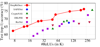
Figure 1: DeepReDuce Pareto frontier of ReLU counts versus accuracy for CIFAR-100. We show DeepReDuce outperforms the state-of-the-art (SAFENet (Lou et al., 2021), CryptoNAS (Ghodsi et al., 2020) and DELPHI (Mishra et al., 2020)).

Prior work has established two methods for private inference. The primary difference between them is how linear layers are computed, either with secret-sharing (SS), a type of secure multi-party computation (MPC) (Goldreich et al., 2019; Shamir, 1979), or homomorphic encryption (HE), an encryption scheme that enables computation on ciphertexts (Gentry et al., 2009; Brakerski & Vaikuntanathan, 2014). For example, Gazelle (Juvekar et al., 2018) and Cheetah (Reagen et al., 2021) use HE for convolution and fully-connected layers whereas MiniONN (Liu et al., 2017), DELPHI (Mishra et al., 2020), and CryptoNAS (Ghodsi et al., 2020) use SS. While distinct, both offer limited functional support and cannot readily process non-linear operations, e.g., ReLUs. To overcome this limitation, private inference protocols use Garbled circuits (GCs), another form of MPC (Yao, 1982, 1986), to process ReLU privately. However, GCs are several orders of magnitude more expensive than the linear layer protocols in terms of communication and computational, rendering private inference impractical (Ghodsi et al., 2020). For example, ReLUs account for 93% of ResNet32’s online private inference time using the DELPHI protocol (Mishra et al., 2020). Therefore, enabling low-latency private inference is a matter of minimizing a network’s ReLU count.

To optimize networks for ReLU count we propose ReLU dropping. Inspired by weight and channel pruning methods that improve plaintext inference speed by reducing FLOPs, ReLU dropping directly reduces ReLU counts by removing entire ReLU layers from the network. While weight and channel pruning also reduce ReLU counts, their ReLU savings are modest compared to FLOP savings. In contrast, ReLU dropping achieves large reductions in ReLU counts by removing ReLU layers wholesale. Leveraging our observations that ReLU operators are unevenly distributed across network layers and contribute differently to accuracy, we find ReLU dropping can be effectively applied to networks for large ReLU count reductions with minimal impact on accuracy.

To further improve results we synergistically combine ReLU dropping with knowledge distillation (KD) (Hinton et al., 2015; Wang & Yoon, 2021) to maximize the accuracy of optimized networks using the original Full-ReLU network. We refer to our overall methodology as DeepReDuce, which includes both optimizations for ReLU dropping and KD training. Figure 1 compares DeepReDuce against the current state-of-the-art: SAFENet (Lou et al., 2021), a method for selectively replacing channel-wise ReLUs with multiple degree and layer-wise mixed precision polynomials; CryptoNAS (Ghodsi et al., 2020), a neural architecture search (NAS) method targeting private inference and DELPHI (Mishra et al., 2020) a method for selectively substituting layer-wise ReLU activations with degree two polynomial activation functions. We find that DeepReDuce significantly advances the accuracy-ReLU budget Pareto frontier across a wide design space.

ReLU dropping has the added benefit that when ReLUs are removed, the now adjacent linear transformations can be combined or merged, reducing the model depth and overall computations, i.e., FLOPs. One obvious alternative to ReLU dropping is to simply start with shallower networks. Our experiments show that DeepReDuce outperforms training shallower networks. For example, ResNet9 (a down-scaled version of ResNet18, details in Section 5) uses 30,720 ReLUs and and achieves 66.2% accuracy whereas DeepReDuce produces a network with both fewer ReLUs (24,600 ReLUs) and higher accuracy (68.1%). We believe this is due to the fact that large models train better, which was also observed in (Zhao et al., 2018). Detailed discussion is included in Section 5.3.

This paper makes the following contributions:

1. Motivate the proposed idea of ReLU dropping and develop DeepReDuce: a method for the judicious removal of ReLUs to optimize networks for fast and accurate private inference.

2. Rigorous evaluation of DeepReDuce demonstrating Pareto optimal designs across a wide range of accuracy and ReLU counts. DeepReDuce improves accuracy up to 3.5% (iso-ReLU count) and reduces ReLUs by 3.5$\times$ (iso-accuracy) over the state of the art.

3. Show existing techniques for neural inference efficiency are insufficient for ReLU reduction and private inference. E.g., compared to the state-of-the-art channel pruning technique (He et al., 2020), DeepReDuce provides a 2$\times$ greater ReLU reduction at with similar accuracy.

2 Motivating ReLU Dropping

In this section we motivate and present the key intuition behind ReLU dropping. We begin by defining the terms relevant to our discussion.

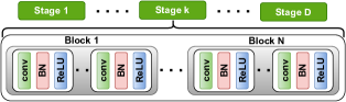
Figure 2: The structure of conventional ResNet-like architectures: Stages comprise Blocks and Blocks comprise multiple repetitions of conv, BN, and ReLU layers.

2.1 Notation

Many state-of-art DNNs have a well defined hierarchy, which allows them to easily scale to different design points (He et al., 2016; Zagoruyko & Komodakis, 2016b; Xie et al., 2017; Huang et al., 2017, 2018; Brendel & Bethge, 2019; Sandler et al., 2018). These architectures consist of multiple Stages ($S$) and each Stage contains copies of the same Block ($B$), as shown in Figure 2. It is typical to call out the first convolution layer as Conv1, which we also do here. The spatial resolution of the feature maps (fmaps) is same within a Stage. For example, the ResNet18 architecture contains four Stages, each with two residual Blocks where residual Blocks constitute two $3\times 3$ convolution layers (He et al., 2016). Conventional scaling methods for designing smaller networks include channel and feature map scaling. Channel scaling reduces the dimensions of the weights by a factor $\alpha$ and feature map scaling reduces the input resolution by $\rho$ (Howard et al., 2017; Tan & Le, 2019).

When describing a DeepReDuce optimized network we explicitly name stages with ReLUs intact. E.g., $S_{2}+S_{3}$ implies stages $S_{1}$ and $S_{4}$ have their ReLUs completely removed and only $S_{2}$ and $S_{3}$ have ReLUs. When a stage is optimized with ReLU Thinning (see below for details) we superscript it with $RT$, e.g., $S_{2}^{RT}$. When channel and feature maps’ resolution scaling are applied we specify $\rho$ and $\alpha$ amounts.

Table 1: ReLUs’ criticality evaluation: ReLU counts and accuracy (CIFAR-100) for ResNet models where ReLUs are dropped from all but one stage. We posit that less accurate ReLU stages indicate less important ReLUs and note accuracy differs significantly across stages.

Models	Metrics	No ReLUs	Conv1	$S_{1}$	$S_{2}$	$S_{3}$	$S_{4}$
ResNet18	#ReLUs	0	66K	262K	131K	66K	33K
	W/o KD (%)	18.49	46.22	61.93	67.63	67.41	58.90
	W/ KD (%)	18.34	45.07	59.85	68.79	69.92	63.16
ResNet34	#ReLUs	0	66K	393K	262K	197K	49K
	W/o KD(%)	18.16	45.42	60.77	69.47	70.04	57.44
	W/ KD(%)	18.07	45.13	62.88	70.93	72.61	64.23

2.2 ReLU Dropping

We now discuss four observations motivate ReLU dropping and DeepReDuce.

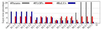
Figure 3: Layer-wise distribution of parameters, FLOPs, and ReLUs in ResNet18. FLOPs are evenly distributed, parameters (ReLUs) are increases (decreases) with network’s depth.

Observation 1: ReLUs are unevenly distributed across the layers of conventional CNNs. We begin by investigating the distribution of ReLUs across the layers of modern CNN architectures. Figure 3 presents a layer-wise breakdown of ResNet18’s ReLUs, FLOPS, and parameters. We observe that FLOPs are evenly distributed across layers, and that the number of ReLUs per layer decreases with depth while the parameter count increases with depth. A similar distribution of parameters, FLOPs, and ReLUs have been observed in other common CNNs (Figure 7 in Appendix E).

The skewed distribution of ReLUs is because conventional CNN architectures tend to scale the number of channels up by $2\times$ and the fmap spatial dimension down by $2\times$ in each dimension across stages, resulting in a $2\times$ drop in ReLU count across a down-sampling layer. All other Things being equal, this presents an opportunity to significantly reduce ReLU counts by simply dropping them from early stages. This fortuitous as we also observe ReLUs in the early stages tend to be less critical for accuracy.

Observation 2: ReLUs in some stages are more important for accuracy than others. To understand the relative importance of ReLUs in different network stages we crafted ablation experiments. This was done by removing ReLUs from all but one ResNet18 stage and training each resulting network from scratch. Table 1 shows the accuracy and ReLU count of each resulting network using the CIFAR-100 dataset. Recall that ResNet18 has Conv1 layer prior to stage 1. For completeness (in Table 1) we report result for ResNet18 with ReLUs only in Conv1. However, we always drop ReLUs from Conv1 along with stages in the network in subsequent experiments.

We note that the four resulting networks vary greatly with respect to accuracy. Networks with ReLUs in $S_{2}$ and $S_{3}$ (Table 1) have high accuracy, even though $S_{2}$ and $S_{3}$ use fewer ReLUs than $S_{1}$. Similarly, although Conv1 and $S_{3}$ have the same number of ReLUs, allocating ReLUs to $S_{3}$ instead of Conv1 increases accuracy by 24.8%. A similar ReLU-accuracy disparity was observed for ResNet34 (see Table 1.) We conclude that not all ReLUs are equal: some contribute more to model accuracy than others. We hypothesize these less important ReLUs can be removed without significantly impacting network’s accuracy.

Observation 3: Some ReLUs benefit more from knowledge distillation that others. Given the disparate impact of dropping ReLUs from stages in a network, we also investigated whether some stages benefit more from KD than others. As illustrated in the Table 1, the accuracy gain from KD is position dependent and greater for networks with ReLUs in deeper stages ($S_{4}$ and $S_{3}$) compared to the networks with ReLUs in initial stages ($S_{1}$ and $S_{2}$). Our results thus suggest that KD is synergistic with ReLU dropping: dropping ReLUs from early layers dramatically reduces ReLU count with a relatively small impact on accuracy and would not have benefited as much from KD had ReLUs in these layers been preserved. Conversely, latter layers with a small number of more critical ReLUs also benefit the most from KD. This resonates with the claim made in (Gotmare et al., 2019) as knowledge shared by a teacher in KD is primarily disbursed in deeper layers.

Table 2: Performance comparison of channel scaling ($\alpha$=0.5) and dropping ReLUs from alternate layers (S${}_{k}^{RT}$ where $k$ is the network stage) using ResNet18 on CIFAR-100. Both methods reduce ReLUs by a factor of 2$\times$; however, alternate ReLU dropping results in more accurate iso-ReLU networks.

Network	#Conv	#ReLUs	W/o KD(%)	W/ KD(%)
$S_{2}$+$S_{3}$+$S_{4}$	17	229K	73.14	76.22
$S_{2}^{RT}$+$S_{3}^{RT}$+$S_{4}^{RT}$	17	115K	72.97	74.72
$S_{2}$+$S_{3}$+$S_{4}$, $\alpha$=0.5	17	115K	71.59	73.78
$S_{2}$+$S_{3}$	17	197K	72.77	75.51
$S_{2}^{RT}$+$S_{3}^{RT}$	17	98K	70.97	71.95
$S_{2}$+$S_{3}$, $\alpha$=0.5	17	98K	69.54	71.16
$S_{3}$+$S_{4}$	17	98K	68.4	73.16
$S_{3}^{RT}$+$S_{4}^{RT}$	17	49K	69.62	71.06
$S_{3}$+$S_{4}$, $\alpha$=0.5	17	49K	66.43	70.29

Observation 4: Dropping ReLUs within stages is better than channel scaling. Our final observation relates to the relative importance of ReLUs within network stages. We explore two strategies for $2\times$ ReLU reduction in a stage: (i) drop ReLUs from alternate layers or (ii) reduce the number of channels in the stage by $2\times$. Table 2 compares alternate layer ReLU dropping against channel down scaling for three different network architectures obtained by dropping ReLUs in $S_{1}$, $S_{1}+S_{4}$, and $S_{1}+S_{2}$. In each instance we observe that at iso-ReLU, alternate layer ReLU dropping has $1\%-3\%$ accuracy improvements over channel down-scaling. We note that even with KD alternate layer ReLU dropping is consistently better than channel down-scaling.

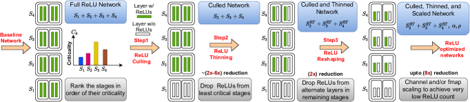
Figure 4: The DeepReDuce ReLU optimization pipeline. The baseline is optimized left to right following orange arrows. Green (plain) boxes indicate layer’s with (without) ReLUs, gray boxes indicate profiling steps to guide optimizations, and blue boxes describe the resulting network after each optimization step. Given a baseline network, DeepReDuce outputs ReLU-optimized networks preserving as much accuracy from the baseline network as possible.

3 DeepReDuce

Using the insights listed above, this section presents the proposed ReLU optimizations and resulting method for optimizing networks for private inference. Given a baseline network as input, DeepReDuce outputs a set of Pareto optimal networks that trade accuracy and ReLU count. This is done via three ReLU reducing optimizations (shown as Step 1 to 3 in Figure 4): Culling (Section 3.1), Thinning (Section 3.2), and Reshaping (Section 3.3). The optimizations work at different levels of granularity and are applied sequentially to identify high-performing networks quickly.

3.1 ReLU Culling

The first optimization, named ReLU Culling, removes ReLUs at a coarse granularity (Step 1 in Figure 4). It works by completely removing all ReLUs from a given network stage. Culling is applied iteratively, from least to most critical using a criticality metric (described below) that estimates the importance of each stage’s ReLUs. Empirically we find the initial stage tends to be highly amenable to Culling as it contains a large number of non-critical ReLUs. For a network with $D$ stages, ReLU Culling outputs $D-1$ networks that trade accuracy for reduced ReLU counts.

Criticality metric: The order that a network’s stages are culled is determined by estimating ReLU criticality, i.e., how important a particular stage’s ReLUs are for accuracy. We denote each stage’s ($S_{k}$) criticality as $C_{k}$. To determine criticality, we first remove all the ReLUs from all network stages except $S_{k}$, train the network, measure its accuracy, and then repeat the process with KD using the original network as a teacher. The criticality metric $C_{k}$ captures the accuracy improvement from retaining ReLUs in stage $S_{k}$ and the stage’s ReLU cost as follows:

$$C_{k}=\frac{Acc[S_{k}]-\min_{(i=1\;to\;D)}\{Acc[Si]\}}{(\#ReLU[S_{k}])^{w}}$$ (1)

In Equation 1, $Acc[S_{k}]$ is the accuracy of the network with ReLUs only in stage $S_{k}$ trained with KD. $\#ReLU[S_{k}]$ in the denominator is the number of ReLUs in stage $S_{k}$. The hyper-parameter $w$ controls the weighted importance of accuracy and ReLU count, we set $w$=0.07, similar to (Tan & Le, 2019). The value of $C_{k}$ corresponding to least critical stage would be zero (see Table 3) and stages with higher $C_{k}$ utilize ReLUs better than stages with lower $C_{k}$. Hence, they are more critical and dropped later in DeepReDuce. We note that, even for the same network, criticality of ReLUs varies across different datasets. For instance, as shown in Table 3 the criticality order of ResNet18 on CIFAR-100, from least to most critical, is $S_{1}<S_{4}<S_{2}<S_{3}$ (calculated from the Table 1); whereas, the same on TinyImageNet is $S_{1}<S_{2}<S_{4}<S_{3}$.

3.2 ReLU Thinning

To further reduce ReLU counts, each Culled network from the ReLU Culling stage is further Thinned by dropping alternate ReLU layers in the remaining non-Culled stages of the network (Step 2 in Figure 4). This yields an additional reduction in ReLU counts for each Culled networks as the number of ReLU layers are halved.

Note that the same reduction in ReLU counts can be achieved via other means, for example, by dropping ReLUs from the first half or last half of a stage, or by scaling the number of channels in each layer by $2\times$. However, we empirically find that ReLU Thinning consistently outperforms both approaches (see results in Section 2). Moreover, our empirical findings resonate with the observations made in (Zhao et al., 2018), which claims that removing ReLUs from alternate layers regularize the network and prevent information loss.

While Thinning could be generalized to drop ReLUs from arbitrary layers in non-Culled stages, this would significantly increase search complexity. Our choice of dropping ReLUs from alternate layers in non-Culled stages is to strike a balance between run-time and effectiveness of DeepReDuce.

Table 3: ReLUs’ Criticality on TinyImageNet for ResNet18/34. FR is baseline with Full-ReLU ($S_{1}$+$S_{2}$+$S_{3}$+$S_{4}$). Similar to the our observations on CIFAR-100 in Table 1, accuracy differs significantly across stages and $S_{1}$ ($S_{3}$) ReLUs are least (most) critical.

Net	ResNet18				ResNet34
	#ReLUs	W/o KD(%)	W/ KD(%)	$C_{k}$	#ReLUs	W/o KD(%)	W/ KD(%)	$C_{k}$
FR	2228K	61.28	-	-	3867K	63.06	-	-
$S_{1}$	1049K	41.90	39.61	0.00	1573K	42.10	39.4	0.00
$S_{2}$	524K	50.53	49.44	6.04	1049K	53.49	51.74	7.58
$S_{3}$	262K	51.93	54.34	9.50	786K	57.28	60.83	13.44
$S_{4}$	131K	46.89	51.46	8.02	197K	48.10	54.41	10.37

3.3 ReLU Reshaping

The final optimization of DeepReDuce uses conventional channel and fmaps resolution scaling to decrease ReLU counts by reducing network size and shape (Step 3 in Figure 4). While less effective than Culling and Thinning, as they tend to introduce higher accuracy drop, these optimization are useful in producing networks for highly-constrained ReLU budgets.

To down-scale networks we explore three alternatives: channel scaling, feature map (fmap) scaling, and compound scaling. Channel and fmap-resolution scaling reduce the filter count and spatial dimensions of fmaps across the network by factors of $\alpha$ and $\rho$, respectively. Compound scaling scales both channels and fmap spatial dimensions simultaneously, achieving multiplicative reductions in ReLU count. More precisely, channel and fmap resolution scaling by $\alpha$ and $\rho$ reduce the ReLU count by $\alpha$ and $\rho^{2}$ respectively. Since our aim is to gradually reduce the ReLU count, we first employ channel scaling ($\alpha$=0.5) and then fmap scaling ($\rho$=0.5) followed by compound scaling ($\alpha$=0.5 and $\rho$=0.5) to reduce the ReLU count by 2$\times$, 4$\times$, and 8$\times$, respectively.

One can use different scaling factors for different degree of ReLU reduction. However, naively selected scaling factors could result in suboptimal ReLU networks. For instance, $\alpha$=0.25 and $\rho$=0.5 both lower the ReLU count by 4$\times$; however, the former produces less accurate networks (see accuracy with KD in Table 9 in Appendix A). One possible explanation for the lower accuracy in channel-scaled networks can be the lower parameter count. That is, while $\alpha$=0.25 and $\rho$=0.5 reduces the ReLU count by same degree the former also reduces the parameter count by 4$\times$, which can reduce the expressiveness of the network.

We note that because Reshaping is applied to all stages equally, it scales down the sizes of critical layers as well. As such, applying Reshaping earlier would reduce opportunities for our more effective Culling and Thinning optimizations. This is why we use Reshaping only as a last resort to reduce ReLU count.

3.4 Improving accuracy using KD

To maximize the accuracy of Culled, Thinned, and Reshaped networks we employ knowledge distillation (KD) as the final step of DeeReDuce. Specifically, we re-train ReLU-optimized networks with Full-ReLU baseline as a teacher, and find distillation typically recovers several percentage points of accuracy on our datasets. We note that although KD is only explicitly used as a final step, it is implicitly incorporated in the evaluation of stage criticality (see Section 3.1), and guides the selection of which stages to Cull first (or last). Since the gain in accuracy from KD depends on the position of stages (Table 1 and 3), order of stage criticality computed with KD is different compared to that computed without KD. Therefore, incorporating KD ($Acc[S_{k}]$ in Eq. 1) in computing criticality produces better results.

3.5 Putting it All Together

We developed DeepReDuce to effectively apply the above optimizations without exhaustively exploring the design space. Given a network as input, DeepReDuce first determines the criticality of each stage. We use this information to guide the application of coarse-grained ReLU Culling. DeepReDuce iteratively applies Culling to each network stage from least to most critical. The application of Culling is compounded after each iteration, e.g., if S₂ was Culled first and S₃ is the next least critical stage, then DeepReDuce Culls both S₂ and S₃ in the following iteration.

Complexity of DeepReDuce: For each iteration Culling, Thinning, and Reshaping are applied individually, resulting in five optimized networks per optimization iteration. Figure 4 shows a single (initial) iteration of DeepReDuce. DeepReDuce explores 5$\times(D-1)$ network architectures as we never Cull the most critical stage. Note that, irrespective of the depth of network, the number of stages varies between 3 to 5. In contrast, the NAS-based architecture search methods, including CryptoNAS, explore a large design space and train significantly more models. Thus, DeepReDuce is more efficient and effective than existing techniques.

4 Methodology

Network architecture: We apply DeepReDuce to standard ResNet18/34 architectures as defined in (He et al., 2016), and also, on the non-residual networks VGGNet (Simonyan & Zisserman, 2014) and MobileNets (Howard et al., 2017).

To show DeepReDuce networks outperform shallower ResNets we trained ResNet10 and ResNet9 in Table 7. In these networks we removed half of the residual Blocks in each stage of ResNet18 (each stage now has only one residual Block). Furthermore, for ResNet9, there is only one $3\times 3$ convolution layer in the first residual Block of $S_{1}$. All other comparisons with state-of-the-art use reported results from respective papers.

Table 4: Optimizations applied (Culling, Thinning, and Reshaping) to Pareto points in Figure 1. Stages with “^⋆” have only one Block inside the ReLU-stages. Acc. is top-1 accuracy for ResNet18 on CIFAR-100, and Lat. is inference time in seconds.

Culled	Thinning	ReLU Reshaping		#ReLUs	Acc.(%)	Lat.(s)	Acc./ReLU
		Ch.	Fmap
ResNet18 baseline model: #ReLUs = 557.06K, top-1 accuracy (W/o KD) = 74.46%
$S_{1}$	NA	NA	NA	229.38K	76.22	4.61	0.332
$S_{1}$+$S_{4}$	NA	NA	NA	196.61K	75.51	3.94	0.384
$S_{1}$	$S_{2}$+$S_{3}$+$S_{4}$	NA	NA	114.69K	74.72	2.38	0.651
$S_{1}$	$S_{2}$+$S_{3}$+$S_{4}$	0.5$\times$	NA	57.34K	72.68	1.37	1.27
$S_{1}$+$S_{4}$	$S_{2}$+$S_{3}$	0.5$\times$	NA	49.15K	69.50	1.19	1.45
$S_{1}$	$S_{2}$+$S_{3}$+$S_{4}$	NA	0.5$\times$	28.67K	68.68	0.74	2.40
$S_{1}$+$S_{4}$	$S_{2}$+$S_{3}$	0.5$\times$	NA	24.57K	68.41	0.56	2.78
$S_{1}$	$S_{2}$+$S_{3}$+$S_{4}$	0.5$\times$	0.5$\times$	14.33K	65.36	0.52	4.56
$S_{1}$+$S_{4}$	$S_{2}$+$S_{3}$	0.5$\times$	0.5$\times$	12.28K	64.97	0.45	5.29
$S_{1}$	$S_{2}^{\star}$+$S_{3}^{\star}$+$S_{4}^{\star}$	0.5$\times$	0.5$\times$	7.17K	62.30	0.21	8.69

Training process: Networks are trained using the following parameters: an initial learning rate of $0.1$, mini-batch size of 128, the momentum of $0.9$ (fixed), and $0.0004$ weight decay factor. We train networks for 120 epochs on both CIFAR-100 and TinyImageNet datasets. The learning rate is reduced by a factor of $10$ every $30^{th}$ epoch. For training on CIFAR-10, we use cosine learning and train the networks for 150 epochs.

When using knowledge distillation, we set the hyper-parameters, temperature and relative weight to cross-entropy loss on hard targets as $4$ and $0.9$, respectively (Hinton et al., 2015; Zagoruyko & Komodakis, 2016a; Cho & Hariharan, 2019). For a fair comparison, we train all the networks with the same hyper-parameters and use the baseline model (without any ReLU dropping) as the teacher during KD. For example, all the DeepReDuce-optimized ResNet18 networks and smaller ResNets, such as ResNet10 and ResNet9, are trained with the baseline Full-ReLU ResNet18 as a teacher.

Table 5: Optimizations steps (Culling, Thinning, and Reshaping) for ReLU-optimized ResNet18 networks on TinyImageNet. Stages with “^⋆” have only one Block inside the ReLU-stages. Acc. is top-1 accuracy, and Lat. is inference time in seconds.

Culled	Thinning	ReLU Reshaping		#ReLUs	Acc.(%)	Lat.(s)	Acc./ReLU
		Ch.	Fmap
ResNet18 baseline model: #ReLUs = 2228.24K, top-1 accuracy (W/o KD) = 61.28%
$S_{1}$	NA	NA	NA	917.52K	64.66	17.16	0.070
$S_{1}$	$S_{2}$+$S_{3}$+$S_{4}$	NA	NA	458.76K	62.26	8.87	0.136
$S_{1}$+$S_{2}$	NA	NA	NA	393.24K	61.65	7.77	0.157
$S_{1}$	$S_{2}$+$S_{3}$+$S_{4}$	0.5$\times$	NA	229.38K	59.18	4.61	0.258
$S_{1}$+$S_{2}$	$S_{3}$+$S_{4}$	NA	NA	196.62K	57.51	4.16	0.292
$S_{1}$	$S_{2}$+$S_{3}$+$S_{4}$	NA	0.5$\times$	114.69K	56.18	2.47	0.490
$S_{1}$+$S_{2}$	$S_{3}$+$S_{4}$	0.5$\times$	NA	98.31K	55.67	2.64	0.566
$S_{1}$	$S_{2}$+$S_{3}$+$S_{4}$	0.5$\times$	0.5$\times$	57.35K	53.75	1.85	0.937
$S_{1}$+$S_{2}$	$S_{3}$+$S_{4}$	NA	0.5$\times$	49.16K	49.00	1.325	0.997
$S_{1}$	$S_{2}^{\star}$+$S_{3}^{\star}$+$S_{4}^{\star}$	0.5$\times$	0.5$\times$	28.67K	47.55	0.678	1.658
$S_{1}$+$S_{2}$	$S_{3}$+$S_{4}$	0.5$\times$	0.5$\times$	24.58K	47.01	0.579	1.913
$S_{1}$+$S_{2}$	$S_{3}^{\star}$+$S_{4}^{\star}$	0.5$\times$	0.5$\times$	12.29K	41.95	0.455	3.414

Dataset: We perform our experiments on the CIFAR-100 (Krizhevsky et al., 2012) and TinyImageNet (Le & Yang, 2015; Yao & Miller, 2015) datasets. CIFAR-100 has 100 output classes with 100 training and test images (resolution $32\times 32$) per class. TinyImageNet has 200 output classes with 500 training and 50 test/validation images (resolution $64\times 64$) per class. We note that prior work on private inference (Mishra et al., 2020) has largely used smaller datasets like MNIST and CIFAR-10 in their evaluations, largely because the high costs of private inference make evaluations on large-scale images difficult.

Private inference protocol: We use the DELPHI (Mishra et al., 2020) protocol for private inference. DELPHI uses a secret sharing for linear layers and garbled circuits (GC) for ReLU layers. DELPHI optimizes the linear layer computations by moving cryptographic operations to an offline (preprocessing) phase. The protocol creates secret shares of the model weights during the offline phase (known before the client’s input is available) and performs all linear operations over secret-shared data during the online phase.

Threat model: We assume the same system setup and threat model as used by DELPHI (Mishra et al., 2020), MiniOnn (Liu et al., 2017), and CryptoNAS (Ghodsi et al., 2020). This model assumes an honest-but-curious adversary. We refer the interested reader to the referenced work for more details as we make no protocol changes and provide the exact same security guarantees.

5 Results

5.1 DeepReDuce Pareto Analysis

Figure 1 shows that DeepReDuce advances the ReLU count-accuracy Pareto frontier. In this section, we present a detailed analysis and quantify the benefit of networks along the frontier. Table 4 shows the details of the DeepReDuce Pareto points in Figure 1. Pareto points are shown in order of highest to lowest accuracy. The primary takeaway from the table is that each of our optimizations (Culling, Thinning and Reshaping) are represented on the Pareto front, indicating that each is critical to obtaining the best results. Second, as mentioned in Section 3.3, Reshaping optimizations are most helpful at lower ReLU budgets, while Culling and Thinning dominate higher ReLU budget points. This observation reaffirms that the order we apply our optimizations performs well.

We focus on CIFAR-100 first to best compare against prior work. Table 5 provides the same data using the TinyImageNet dataset for ResNet18 and the criticality evaluation results are shown in Table 3. The data validates the effectiveness and hints at the general applicability of DeepReDuce. Similar to the CIFAR-100 results, we found ReLUs in the initial layer (e.g., $S_{1}$) to be least critical while ReLUs in the intermediate layers (specifically ReLUs in penultimate stage) are most critical.

Accuracy per ReLU: Given that ReLU minimization and accuracy are competing objectives, it is interesting to understand network design tradeoffs as accuracy per ReLU. In the final column of Table 4 and Table 5 we report each networks’ accuracy per kilo-ReLU on CIFAR-100 and TinyImageNet datasets. When ranking networks with respect to ReLU count (highest to lowest), we observe accuracy per ReLU increases as ReLU count decreases. In the extreme, the worst performing CIFAR-100 network (Table 4) is 13.9% less accurate than the most accurate network but also uses 32$\times$ fewer ReLUs, resulting in 26.2$\times$ more accuracy per kilo-ReLU. Similarly, the lowest accurate network on TinyImageNet (Table 5) is 22.7% less accurate but 74.7$\times$ fewer ReLU count than the most accurate network, resulting in 48.8$\times$ more accuracy per kilo-ReLU.

We believe this is a beneficial property for ReLU optimizations like DeepReDuce. It implies that as fewer ReLUs are used, each contributes more to accuracy, picking up the slack. Moreover, while it takes many ReLUs to train a highly-accurate network, accuracy degrades slowly as significant quantities of ReLUs are dropped. This suggests that a natural robustness to ReLU dropping may be a property of neural networks that designers can leverage to optimize networks for private inference.

Table 6: Comparison of DeepReDuce and the state-of-the-art in private inference: CryptoNAS (Ghodsi et al., 2020) and DELPHI (Mishra et al., 2020). Results show that DeepReDuce strictly outperforms both solutions at various ReLU counts. Acc. is top-1 accuracy on CIFAR-100 and Lat. is inference time in seconds.

	SOTA			DeepReDuce			Improvement
	ReLUs	Acc.(%)	Lat.(s)	ReLUs	Acc.(%)	Lat.(s)	ReLU	Acc.(%)	Lat.(s)
CryptoNAS	344K	75.5	7.50	197K	75.50	3.94	1.75$\times$	0.0	1.9$\times$
	100K	68.7	2.30	28.6K	68.70	0.738	3.5$\times$	0.0	3.1$\times$
	86K	68.1	2.00	28.6K	68.70	0.738	3$\times$	0.6	2.7$\times$
	50K	63.6	1.67	12.3K	65.00	0.455	4$\times$	1.4	3.7$\times$
DELPHI	300K	68	6.5	28.7K	68.70	0.738	10.5$\times$	0.7	8.8$\times$
	180K	67	4.44	24.6K	68.41	0.579	7.3$\times$	1.4	7.7$\times$
	50K	66	1.23	49.2K	69.50	1.19	1$\times$	3.5	1$\times$

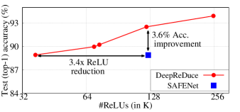
Figure 5: Performance comparison of VGG16 DeepReDuce model and SAFENet on CIFAR-10. The DeepReDuce-optimized VGG16 models outperform SAFENet-optimized VGG16 by a huge margin at both iso-accuracy and iso-ReLU.

5.2 DeepReDuce Outperforms Prior Work

Table 6 shows competing design points for CryptoNAS and DELPHI. We observe that CryptoNAS networks work well for high accuracy, while DELPHI is best for small ReLU budgets. To fairly compare, we only select DeepReDuce points that offer benefit in both accuracy and ReLU count.

Starting with high-accuracy networks, CryptoNAS needs 100K ReLUs to get an accuracy of 68.7%; DeepReDuce is able to match this accuracy using only 28.7K, providing a savings of 3.5$\times$ ReLUs. A DELPHI network needs 300K ReLUs to achieve similar accuracy, which is 10.5$\times$ more ReLUs than DeepReDuce uses. DELPHI is more competitive with networks achieving 67% and 66% accuracy. In fact, DELPHI outperforms CryptoNAS when targeting a 50K ReLU budget, reporting 66% accuracy, while CryptoNAS is only able to realize 63.6% given the same ReLU budget. With a target of 50K ReLUs, DeepReDuce optimizes a network that is (in absolute terms) 3.5% more accurate than DELPHI. Considering the Pareto set of merged DELPHI and CryptoNAS points, DeepReDuce offers a maximum ReLU savings of 3.5$\times$ (iso-accuracy) and a accuracy benefit of 3.5% (iso-ReLU budget). Finally, we note that CryptoNAS compares with and outperforms existing NAS methods for FLOP-optimized network design, and by extension DeepReDuce outperforms these methods as well.

We further compare DeepReDuce to SAFENet, a recently proposed (Lou et al., 2021) fine-grained, channel-wise ReLU optimization targeting ReLU-heavy layers. SAFENet works by selectively substituting ReLUs with polynomials and uses different polynomials and approximation ratios across layers. Comparing the online latency for ResNet on CIFAR-100, we find DeepReDuce is 12.86$\times$ faster (0.56s vs 7.2s) and 1.18% more accurate (68.68% vs 67.5%). For VGG16 on CIFAR-10, SAFENet reports 88.9% accuracy with 56% ReLUs approximated; even assuming all SAFENet approximated ReLUs are free, DeepReDuce provides a 3.4$\times$ ReLU reduction at iso-accuracy and 3.6% more accuracy at iso-ReLU count (Figure 5). The criticality evaluation for VGG16 and optimization steps for the DeepReDuce Pareto points shown in Figure are 5 are listed in Table 10 and 11, respectively, in Appendix B.

Table 7: A comparison of DeepReDuce against smaller ResNet models on CIFAR-100. Results show that, iso-ReLU count and iso-accuracy, DeepReDuce consistently outperforms smaller ResNets.

Network	#Conv	#ReLUs	W/o KD(%)	W/ KD(%)
ResNet10, $\alpha$=0.5	9	155.6K	71.3	72.5
$S_{2}^{RT}$ + $S_{3}$ + $S_{4}^{RT}$	17	147.6K	71.7	74.8
ResNet10, $\rho$=0.5	9	47.1K	64.7	68.1
$S_{2}^{RT}$ + $S_{3}^{RT}$	11	49.2K	67.8	71.0
ResNet9, $\alpha$=0.5, $\rho$=0.5	8	30.7K	62.6	66.2
$S_{2}^{RT}$ + $S_{3}^{RT}$ + $S_{4}^{RT}$, $\rho$=0.5	8	28.7K	64.4	68.5
$S_{2}^{RT}$ + $S_{3}^{RT}$, $\alpha$=0.5	7	24.6K	66.0	68.1

5.3 DeepReDuce Outperforms Shallow ResNets

DeepReDuce’s Culling and Thinning optimizations effectively reduce network depth. Thus, it is natural to ask why not simply train a smaller network? We compared DeepReDuce against standard ResNet architectures with similar depth and ReLU counts. To compare fairly, we start with a baseline ResNet18 model and scale it down to match the ReLU counts of DeepReDuce networks (see Section 4 for details). To compare the performance at both iso-Layer and iso-ReLU, we merge the linear layers/Blocks in DeepReDuce networks at inference time. Since DeepReDuce uses KD, we also apply it to scaled ResNets for fair comparison. The results are shown in Table 7.

We first show that DeepReDuce outperforms ResNet10 models using both fmap and channel scaling. When given the same number of layers (see bold row), DeepReDuce uses two thousand fewer ReLUs and is 2.3% more accurate than ResNet9. DeepReDuce uses fewer convolution layers when dropping a ReLU connecting two convolutions layers, which allows them to be combined or merged. Moreover, we can continue to scale down DeepReDuce to use fewer ReLUs (24.6K) and still be 1.9% more accurate than the smaller ResNet9 model. Thus, we conclude that DeepReDuce outperforms simply training smaller networks.

5.4 DeepReDuce Outperforms Channel Pruning

While DeepReDuce and channel pruning have different optimization objectives, channel pruning also reduces ReLUs. We compare DeepReDuce with a recent state-of-art channel pruning method (He et al., 2020) and compare the two methods in terms ReLUs, FLOPs, and accuracy. Since authors in aforementioned paper report results using ResNet56 as the baseline, we ran DeepReDuce on the same network. (Table 14 in Appendix D shows the per-stage criticality for ResNet56; stage $S1$ ($S3$) is the least (most) critical stage for this network.)

Table 8 compares DeepReDuce with channel pruning on the CIFAR-10 and CIFAR-100 datasets. DeepReDuce has the higher accuracy (0.73% and 2.83% more accurate on CIFAR-10 and CIFAR-100, respectively) and uses $1.4\times$ fewer ReLUs compared to channel pruning. At a slightly lower accuracy (0.18% less) on CIFAR-10, DeepReDuce’s reduction in ReLUs over channel pruning increases to more than $2\times$ (147.5K vs. 311.7K).

DeepReDuce performs even better on CIFAR-100. It is 1% more accurate (71.68% vs. 70.83%) with 2$\times$ fewer ReLUs compared to channel pruning. In all our comparisons we observed that DeepReDuce has $~{}1.4\times$ more FLOPs compared to channel pruning; this is not a problem for DeepReDuce because FLOPs are effectively free for private inference run-time as noted by (Ghodsi et al., 2020). We conclude that FLOP-count oriented network optimizations are very different from ReLU-oriented network optimizations.

Table 8: Performance comparison of channel pruning (He et al., 2020) and DeepReDuce for FLOPs and ReLU saving, and accuracy drop on ResNet56 with CIFAR-10 (C10) and CIFAR-100 (C100) datasets. DeepReDuce models save significantly higher #ReLUs at similar FLOPs saving and accuracy drop.

	Method	Baseline Acc.(%)	Pruned Acc.(%)	Acc. $\downarrow$(%)	FLOPs	ReLUs
C10	Ch. pruning	93.59	93.34	-0.25	59.1M	311.7K
	DeepReDuce	93.48	94.07	+0.59	87.7M	221.2K
			93.16	-0.32	66.5M	147.5K
C100	Ch. pruning	71.41	70.83	-0.58	60.8M	311.7K
	DeepReDuce	70.93	73.66	+2.57	87.7M	221.2K
			71.68	+0.59	66.5M	147.5K

5.5 DeepReDuce Network Inference Latencies

We conclude by showing the inference speedup time improvements offered by DeepReDuce. Experiments were run to measure the latency for DeepReDuce optimized models using the same experimental setup and private inference protocol as DELPHI  (Mishra et al., 2020). Table 4 and Table 5 present latency results of ResNet18 on CIFAR-100 and TinyImageNet, respectively. As expected, we observe that inference latency strongly correlates with a network’s ReLU count. For example, at iso-accuracy (on CIFAR-100), we achieve a 3.7$\times$ latency reduction compared to CryptoNAS. Compared to DELPHI, and assuming iso-latency, DeepReDuce offers 3.5% accuracy improvement on CIFAR-100. The fastest DeepReDuce model on CIFAR-100, i.e., the one with the fewest ReLUs, takes 455mS per inference with an accuracy of 65%. Similarly, on TinyImageNet, we achieve 59.18% top-1 accuracy with a latency of 4.6S. While advancing the state-of-the-art, these inference times are still too high to meet real-time requirements 30-60 FPS (Wu et al., 2019), and more work is needed to achieve the ultimate goal of real-time private inference.

5.6 Generality Case Study: MobileNets

Here we examine the generality of DeepReDuce using MobileNetV1 (Howard et al., 2017). We chose to study MobileNet as it is very different from ResNet—the convolution layers do not use residuals and the Depthwise architecture is FLOP optimized, which we believe is a poor match for the ReLU costs of private inference. We first evaluate the ReLUs’ criticality (see Table 12 in Appendix C) and then compare the performance of ReLU-optimized DeepReDuce models with conventionally (channel/fmap-resolution) scaled MobileNetV1 models. For fair comparison, we use KD for scaled-MobileNetV1 models where teacher is Full-ReLU baseline MobileNetV1 and hence, all the results reported in Figure6 are with KD.

Results are shown in Figure 6 and the optimization steps for all DeepReDuce models are listed in Table 13 in Appendix C. The substantial gain, 10.9% improvement in accuracy at iso-ReLU and 3.8$\times$ ReLU reduction at iso-accuracy (see Figure 6) shows the effectiveness of DeepReDuce ReLU optimization on MobileNetV1.

Thus, while residual connections benefit DeepReDuce, they are not a necessity as DeepReDuce also performs well when residual connections are eliminated from the network and the non-residual networks such as MobileNets and VGG16 (Figure 5).

6 Related Work

CryptoNets (Gilad-Bachrach et al., 2016) was the first to demonstrate using homomorphic encryption to protect client data during inference. SecureML (Mohassel & Zhang, 2017) focuses on privacy-preserving training of several machine learning models, including neural networks using a two-server protocol. While (Mohassel & Zhang, 2017) supports inference as well, it incurs high overheads by relying on generic MPC protocols. MiniONN (Liu et al., 2017) generates multiplication triplets for each multiplication in a linear layer and combines that with GC protocol for ReLU activation functions. Gazelle (Juvekar et al., 2018) uses an optimized HE scheme for linear layers and GC for non-linear layers. DELPHI (Mishra et al., 2020) further optimizes this protocol by moving the heavy cryptographic operations to an offline preprocessing phase and using only secret sharing for linear layers online. In DELPHI, select ReLU layers are replaced with quadratic functions and the authors propose a neural architecture search method (NAS) to determine which ReLU layers to replace. CryptoNAS (Ghodsi et al., 2020) defines a ReLU budget for private inference task and aims to find the best networks for a budget using NAS. A recent work SAFENet (Lou et al., 2021) selectively replaces the channel-wise ReLUs with multiple degree polynomials and uses layer-wise mixed precision.

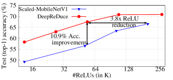
Figure 6: Performance comparison of DeepReDuce models and (channel/fmap-resolution) scaled MobileNetV1 on CIFAR-100. DeepReDuce optimized models outperform the scaled MobileNetV1 by a huge margin at both iso-accuracy and iso-ReLU.

7 Conclusion and Future Work

This paper develops the concept of ReLU dropping as an effective method for tailoring networks for private inference. The DeepReDuce method carefully prioritizes and removes ReLUs based on how critical they are, and users are given a wide range of networks that trade ReLU count and accuracy. Evaluating DeepReDuce on CIFAR-100 shows 3.5% improvement at iso-ReLU and 3.5$\times$ ReLU reduction at iso-accuracy. We also perform the experiments on TinyImageNet, which is uncommon for private inference work given the long runtimes. While we advance the state-of-the-art, we still fall short of the ultimate goal of real-time private inference. We expect DeepReduce to inspire future optimizations and new ways of Thinking about network design to achieve this goal.

Appendix A Channel Scaling Vs. Feature map Scaling

For extremely lower ReLU budgets, we use a combination of channel scaling and fmaps’ resolution scaling. Since reducing fmaps’ resolution (each spatial dimensions of fmaps) by 2$\times$ ($\rho$=0.5) decreases the ReLU count by 4$\times$, we first use channel scaling ($\alpha$ = 0.5) for reducing the ReLU count by 2$\times$. Further, for 4$\times$ reduction in ReLU count, we prefer to use fmaps’ resolution scaling ($\rho$=0.5) over channel scaling ($\alpha$=0.25) since the former results in more accurate networks, as illustrated in Table 9. Unlike fmap resolution scaling, channel scaling reduces the parameter count along with the ReLU count, which may reduce the expressive power of a network. Hence, the network is more accurate with fmaps’ resolution scaling.

Table 9: Performance comparison for ReLU optimization using channel scaling ($\alpha<$1) and fmap-resolution scaling ($\rho<$1). Baseline models have $\alpha$=1 and $\rho$=1. At iso-ReLU, accuracy (w/ KD) of the the fmap-resolution scaled models is higher than the channel scaled models.

Network	#Conv	#ReLUs	CIFAR-100
			W/o KD (%)	W/ KD (%)
ResNet18 (baseline)	17	557K	74.46	76.94
ResNet18; $\alpha$=0.25, $\rho$=1	17	139K	68.17	70.19
ResNet18; $\alpha$=1, $\rho$=0.5	17	139K	68.47	72.72
ResNet10 (baseline)	9	311K	74.10	76.69
ResNet10; $\alpha$=0.25, $\rho$=1	9	78K	66.69	66.88
ResNet10; $\alpha$=1, $\rho$=0.5	9	78K	66.67	71.86
ResNet6 (baseline)	5	188K	68.86	69.58
ResNet6; $\alpha$=0.25, $\rho$=1	5	47K	57.64	56.9
ResNet6; $\alpha$=1, $\rho$=0.5	5	47K	64.74	68.09

Appendix B VGGNet DeepReDuce Pareto Points

We do not remove ReLUs from fully connected (FC) layers as FC account only 8.192K ReLUs and training networks without FC ReLUs is challenging. The results are shown in Table 10. Unlike ResNets and MobileNets, ReLUs in $S_{5}$ are least critical and that of the $S_{1}$ is moderate.

Table 10: Stage-wise ReLUs’ criticality in VGG16 evaluated on CIFAR-10. $S_{5}$ is least critical while $S_{2}$ and $S_{3}$ are most critical.

Net	#ReLUs	W/o KD (%)	W/ KD (%)	$C_{k}$
$S_{1}$ + FC-ReLUs	139.3K	82.0	81.4	10.90
$S_{2}$ + FC-ReLUs	73.7K	86.1	85.3	14.31
$S_{3}$ + FC-ReLUs	57.3K	86.4	85.1	14.40
$S_{4}$ + FC-ReLUs	32.8K	77.1	77.7	9.17
$S_{5}$ + FC-ReLUs	14.3K	63.9	66.0	0.00

The ReLU optimizations step for the Pareto points in Figure 5 are listed in Table 11. Models are the ReLU-optimized versions (Thinned and Reshaped) of two Culled networks: (1) stages $S_{4}$ and $S_{5}$ are Culled and (2) stages $S_{1}$, $S_{4}$ and $S_{5}$ are Culled.

Table 11: Optimization steps for MobileNetV1 DeepReDuce models shown in Figure 5

Optimization Steps	#ReLUs	Acc.(%)
$S_{1}$ + $S_{2}$ + $S_{3}$ + FC	253.95K	93.92
$S_{2}$ + $S_{3}$ + FC	122.88K	92.52
$S_{2}^{RT}$ + $S_{3}^{RT}$ + FC	73.73K	90.23
$S_{1}^{RT}$ + $S_{2}^{RT}$ + $S_{3}^{RT}$ + FC, $\alpha$=0.5	69.63K	89.97
$S_{2}^{RT}$ + $S_{3}^{RT}$ + FC, $\alpha$=0.5	36.86K	88.92

Appendix C ReLUs’ Criticality and Pareto Points for MobileNets

We evaluate the ReLUs’ criticality in MobileNetV1 (Howard et al., 2017) and MobileNetV2 (Sandler et al., 2018)) on the CIFAR-100. The results are shown in Table 12. We observed the similar trend as ResNet18 and ResNet34 on CIFAR-100/TinyImageNet (shown in Tables 1 and 3), accuracy differs significantly across stages and $S_{1}$ ($S_{4}$) ReLUs are least (most) critical.

Table 12: Stage-wise criticality of ReLUs in MobileNetV1 and MobileNetV2 evaluated on CIFAR-100. FR is baseline with Full-ReLU ($S_{1}$+$S_{2}$+$S_{3}$+$S_{4}$+$S_{5}$). ReLUs in $S_{1}$ ($S_{4}$) are least (most) critical.

Net	MobileNetV1				MobileNetV2
	#ReLUs	W/o KD(%)	W/ KD(%)	$C_{k}$	#ReLUs	W/o KD(%)	W/ KD(%)	$C_{k}$
FR	411.6K	67.58	-	-	425.6K	68.46	-	-
$S_{1}$	131.1K	33.06	34.16	0.00	196.6K	37.82	34.25	0.00
$S_{2}$	114.7K	49.64	50.65	11.83	110.6K	49.83	46.93	9.12
$S_{3}$	57.3K	55.56	54.20	15.09	58.4K	54.74	53.06	14.15
$S_{4}$	94.2K	57.37	61.10	19.60	27.6K	57.08	57.28	18.26
$S_{5}$	14.3K	42.32	45.45	9.37	32.4K	48.42	50.49	12.73

The Pareto points of DeepReDuce models for MobileNetV1 (CIFAR-100) are shown in Figure 6. The optimization steps for all DeepReDuce models are list in the Table 13.

First, in step 1 of DeepReDuce (Figure 4), we Culled the least critical stage $S_{1}$. In step 2 of ReLU Thinning, we had two ways to remove the ReLUs from alternate layers, either from $3\times 3$ depthwise convolution layer or $1\times 1$ pointwise convolution layer. When downsampling is performed in $3\times 3$ depthwise convolution layer, the ReLU count of both the layers are not equal. More precisely, #ReLUs in the $1\times 1$ pointwise convolution is twice as that in the preceding $3\times 3$ depthwise conv.

We empirically found that removing ReLUs from $3\times 3$ depthwise conv layer yields more accurate iso-ReLU models. We suspect this is because $3\times 3$ depthwise convolutions perform filtering (feature learning) and $1\times 1$ pointwise convolutions perform feature aggregation (Howard et al., 2017), the ReLUs in the former layer is more critical for accuracy.

Table 13: Optimization steps for MobileNetV1 DeepReDuce models shown in Figure 6

Optimization Steps	#ReLUs	Acc.(%)
$S_{2}$ + $S_{3}$ + $S_{4}$ + $S_{5}$	280.60K	70.83
$S_{2}^{RT}$ + $S_{3}^{RT}$ + $S_{4}^{RT}$ + $S_{5}^{RT}$	108.54K	70.77
$S_{2}^{RT}$ + $S_{3}^{RT}$ + $S_{4}^{RT}$ + $S_{5}^{RT}$, $\alpha$=0.5	54.27K	67.46
$S_{2}^{RT}$ + $S_{3}^{RT}$ + $S_{4}^{RT}$ + $S_{5}^{RT}$, $\rho$=0.5	27.14K	62.96
$S_{2}^{RT}$ + $S_{3}^{RT}$ + $S_{4}^{RT}$ + $S_{5}^{RT}$, $\alpha$=0.5, $\rho$=0.5	13.57K	58.25

Appendix D ReLU Criticality in ResNet56

We examine the stage-wise criticality of ReLUs in ResNet56 and results are shown in Table 14.

Table 14: Stage-wise criticality of ReLUs in ResNet56 evaluated on CIFAR-100. $S3$ is most critical and $S1$ is least critical.

Stages	#ReLUs	W/o KD (%)	W/ KD (%)	$C_{k}$
S1	311.3K	57.92	59.45	0.0
S2	147.5K	65.62	67.97	6.0
S3	73.73K	65.36	69.22	7.2

Appendix E Layer-wise Distribution of ReLUs

We show the layer-wise distribution of FLOPs, parameters, and ReLU count in the standard networks such as ResNet34 (He et al., 2016), VGG16 (Simonyan & Zisserman, 2014), MobileNetV1 (Howard et al., 2017), and MobileNetV2 (Sandler et al., 2018) in Figure 7. Consistent with ResNet18 (Figure 3), the FLOPs are evenly distributed, more parameters are used in deeper layers, and ReLUs are mostly in initial layers of the networks. Thus, the ReLU reduction in initial layers has a significantly greater impact on the overall ReLU count of these networks. Moreover, the stark difference between the ReLU distribution and FLOPs/parameter distribution indicates that ReLU optimization cannot be ensured through the popular FLOPs/parameters pruning techniques.

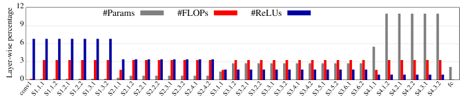
(a) Layer-wise distribution of parameter, FLOPs, and ReLUs in ResNet34 (He et al., 2016).

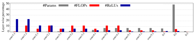
(b) Layer-wise distribution of parameter, FLOPs, and ReLUs in VGG16 (Simonyan & Zisserman, 2014).

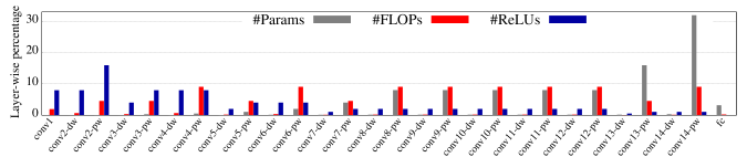
(c) Layer-wise distribution of parameter, FLOPs, and ReLUs in MobileNetV1 (Howard et al., 2017).

Figure 7: Layer-wise percentage of parameter, FLOPs, and ReLUs in various DNNs. FLOPs are evenly distributed, parameters (ReLUs) are increases (decreases) from initial to deeper layers.

References

- Act (1996) Act, A. Health insurance portability and accountability act of 1996, 1996.
- Brakerski & Vaikuntanathan (2014) Brakerski, Z. and Vaikuntanathan, V. Efficient fully homomorphic encryption from (standard) lwe. SIAM Journal on Computing, 43(2):831–871, 2014.
- Brendel & Bethge (2019) Brendel, W. and Bethge, M. Approximating CNNs with bag-of-local-features models works surprisingly well on imagenet. In ICLR, 2019.
- Cho & Hariharan (2019) Cho, J. H. and Hariharan, B. On the efficacy of knowledge distillation. In Proceedings of the IEEE International Conference on Computer Vision, pp. 4794–4802, 2019.
- Gentry et al. (2009) Gentry, C. et al. A fully homomorphic encryption scheme, volume 20. Stanford university Stanford, 2009.
- Ghodsi et al. (2020) Ghodsi, Z., Veldanda, A. K., Reagen, B., and Garg, S. CryptoNAS: Private inference on a relu budget. Advances in Neural Information Processing Systems, 2020.
- Gilad-Bachrach et al. (2016) Gilad-Bachrach, R., Dowlin, N., Laine, K., Lauter, K., Naehrig, M., and Wernsing, J. Cryptonets: Applying neural networks to encrypted data with high throughput and accuracy. In International Conference on Machine Learning, pp. 201–210, 2016.
- Goldreich et al. (2019) Goldreich, O., Micali, S., and Wigderson, A. How to play any mental game, or a completeness theorem for protocols with honest majority. In Providing Sound Foundations for Cryptography: On the Work of Shafi Goldwasser and Silvio Micali, pp. 307–328. 2019.
- Gotmare et al. (2019) Gotmare, A., Keskar, N. S., Xiong, C., and Socher, R. A closer look at deep learning heuristics: Learning rate restarts, warmup and distillation. In ICLR, 2019.
- He et al. (2016) He, K., Zhang, X., Ren, S., and Sun, J. Deep residual learning for image recognition. In Proceedings of the IEEE conference on computer vision and pattern recognition, pp. 770–778, 2016.
- He et al. (2020) He, Y., Ding, Y., Liu, P., Zhu, L., Zhang, H., and Yang, Y. Learning filter pruning criteria for deep convolutional neural networks acceleration. In Proceedings of the IEEE/CVF Conference on Computer Vision and Pattern Recognition, pp. 2009–2018, 2020.
- Hinton et al. (2015) Hinton, G., Vinyals, O., and Dean, J. Distilling the knowledge in a neural network. arXiv preprint arXiv:1503.02531, 2015.
- Howard et al. (2017) Howard, A. G., Zhu, M., Chen, B., Kalenichenko, D., Wang, W., Weyand, T., Andreetto, M., and Adam, H. Mobilenets: Efficient convolutional neural networks for mobile vision applications. arXiv preprint arXiv:1704.04861, 2017.
- Huang et al. (2017) Huang, G., Liu, Z., Van Der Maaten, L., and Weinberger, K. Q. Densely connected convolutional networks. In Proceedings of the IEEE conference on computer vision and pattern recognition, pp. 4700–4708, 2017.
- Huang et al. (2018) Huang, G., Liu, S., Van der Maaten, L., and Weinberger, K. Q. Condensenet: An efficient densenet using learned group convolutions. In Proceedings of the IEEE conference on computer vision and pattern recognition, pp. 2752–2761, 2018.
- Juvekar et al. (2018) Juvekar, C., Vaikuntanathan, V., and Chandrakasan, A. Gazelle: A low latency framework for secure neural network inference. In 27th USENIX Security Symposium (USENIX Security 18), pp. 1651–1669, 2018.
- Krizhevsky et al. (2012) Krizhevsky, A., Nair, V., and Hinton, G. CIFAR-100 (canadian institute for advanced research). 2012. URL http://www.cs.toronto.edu/~kriz/cifar.html.
- Le & Yang (2015) Le, Y. and Yang, X. Tiny imagenet visual recognition challenge. CS 231N, 7, 2015.
- Liu et al. (2017) Liu, J., Juuti, M., Lu, Y., and Asokan, N. Oblivious neural network predictions via minionn transformations. In Proceedings of the 2017 ACM SIGSAC Conference on Computer and Communications Security, pp. 619–631, 2017.
- Lou et al. (2021) Lou, Q., Shen, Y., Jin, H., and Jiang, L. SAFENet: A secure, accurate and fast neural network inference. In ICLR, 2021.
- Mishra et al. (2020) Mishra, P., Lehmkuhl, R., Srinivasan, A., Zheng, W., and Popa, R. A. DELPHI: A cryptographic inference service for neural networks. In 29th USENIX Security Symposium (USENIX Security 20), 2020.
- Mohassel & Zhang (2017) Mohassel, P. and Zhang, Y. Secureml: A system for scalable privacy-preserving machine learning. In 2017 IEEE Symposium on Security and Privacy (SP), pp. 19–38, 2017.
- Reagen et al. (2021) Reagen, B., Choi, W., Ko, Y., Lee, V. T., Lee, H. S., Wei, G., and Brooks, D. Cheetah: Optimizing and accelerating homomorphic encryption for private inference. In IEEE International Symposium on High-Performance Computer Architecture, HPCA, pp. 26–39, 2021.
- Regulation (2016) Regulation, G. D. P. Regulation eu 2016/679 of the european parliament and of the council of 27 april 2016. Official Journal of the European Union., 2016.
- Sandler et al. (2018) Sandler, M., Howard, A., Zhu, M., Zhmoginov, A., and Chen, L.-C. Mobilenetv2: Inverted residuals and linear bottlenecks. In Proceedings of the IEEE conference on computer vision and pattern recognition, pp. 4510–4520, 2018.
- Shamir (1979) Shamir, A. How to share a secret. Communications of the ACM, 22(11):612–613, 1979.
- Simonyan & Zisserman (2014) Simonyan, K. and Zisserman, A. Very deep convolutional networks for large-scale image recognition. arXiv preprint arXiv:1409.1556, 2014.
- Tan & Le (2019) Tan, M. and Le, Q. Efficientnet: Rethinking model scaling for convolutional neural networks. In International Conference on Machine Learning, pp. 6105–6114. PMLR, 2019.
- Wang & Yoon (2021) Wang, L. and Yoon, K.-J. Knowledge distillation and student-teacher learning for visual intelligence: A review and new outlooks. IEEE Transactions on Pattern Analysis and Machine Intelligence, 2021.
- Wu et al. (2019) Wu, C., Brooks, D., Chen, K., Chen, D., Choudhury, S., Dukhan, M., Hazelwood, K., Isaac, E., Jia, Y., Jia, B., Leyvand, T., Lu, H., Lu, Y., Qiao, L., Reagen, B., Spisak, J., Sun, F., Tulloch, A., Vajda, P., Wang, X., Wang, Y., Wasti, B., Wu, Y., Xian, R., Yoo, S., and Zhang, P. Machine learning at facebook: Understanding inference at the edge. In 2019 IEEE International Symposium on High Performance Computer Architecture (HPCA), pp. 331–344, 2019. doi: 10.1109/HPCA.2019.00048.
- Xie et al. (2017) Xie, S., Girshick, R., Dollár, P., Tu, Z., and He, K. Aggregated residual transformations for deep neural networks. In Proceedings of the IEEE conference on computer vision and pattern recognition, pp. 1492–1500, 2017.
- Yao (1982) Yao, A. C. Protocols for secure computations. In 23rd annual symposium on foundations of computer science (sfcs 1982), pp. 160–164. IEEE, 1982.
- Yao (1986) Yao, A. C.-C. How to generate and exchange secrets. In 27th Annual Symposium on Foundations of Computer Science (sfcs 1986), pp. 162–167. IEEE, 1986.
- Yao & Miller (2015) Yao, L. and Miller, J. Tiny imagenet classification with convolutional neural networks. CS 231N, 2(5):8, 2015.
- Zagoruyko & Komodakis (2016a) Zagoruyko, S. and Komodakis, N. Paying more attention to attention: Improving the performance of convolutional neural networks via attention transfer. arXiv preprint arXiv:1612.03928, 2016a.
- Zagoruyko & Komodakis (2016b) Zagoruyko, S. and Komodakis, N. Wide residual networks. arXiv preprint arXiv:1605.07146, 2016b.
- Zhao et al. (2018) Zhao, G., Zhang, Z., Guan, H., Tang, P., and Wang, J. Rethinking relu to train better cnns. In 2018 24th International Conference on Pattern Recognition (ICPR), pp. 603–608. IEEE, 2018.