Extrusion of chromatin loops by a composite loop extrusion factor

Abstract

Chromatin loop extrusion by Structural Maintenance of Chromosome (SMC) complexes is thought to underlie intermediate-scale chromatin organization inside cells. Motivated by a number of experiments suggesting that nucleosomes may block loop extrusion by SMCs, such as cohesin and condensin complexes, we introduce and characterize theoretically a composite loop extrusion factor (composite LEF) model. In addition to an SMC complex that creates a chromatin loop by encircling two threads of DNA, this model includes a remodeling complex that relocates or removes nucleosomes as it progresses along the chromatin, and nucleosomes that block SMC translocation along the DNA. Loop extrusion is enabled by SMC motion along nucleosome-free DNA, created in the wake of the remodeling complex, while nucleosome re-binding behind the SMC acts as a ratchet, holding the SMC close to the remodeling complex. We show that, for a wide range of parameter values, this collection of factors constitutes a composite LEF that extrudes loops with a velocity, comparable to the velocity of remodeling complex translocation on chromatin in the absence of SMC, and much faster than loop extrusion by an isolated SMC that is blocked by nucleosomes.

I Introduction

Exquisite spatial organization is a defining property of chromatin, allowing the genome both to be accommodated within the volume of the cell nucleus, and simultaneously accessible to the transcriptional machinery, necessary for gene expression. On the molecular scale, histone proteins organize 147 bp of DNA into nucleosomes, that are separated one from the next by an additional 5-60 bp [1]. On mesoscopic scales ($10^{5}-10^{6}$ bp), it has long been understood that loops are an essential feature of chromatin organization. The recent development of chromosome conformation capture (Hi-C) techniques now enables quantification of chromatin organization via a proximity ligation assay, that yields a map of the relative probability that any two genomic locations are in contact with each other [2]. Hi-C contact maps have led to the identification of topologically associating domains (TADs) as fundamental elements of intermediate-scale chromatin organization [3, 4, 5, 6, 7]. Genomic regions inside a TAD interact frequently with each other, but have relatively little contact with regions in even neighboring TADs.

Although, how TADs arise remains uncertain, the loop extrusion factor (LEF) model has emerged as the preferred candidate mechanism for TAD formation. In this model, LEFs – identified as the Structural Maintenance of Chromosome (SMC) complexes, cohesin and condensin – encircle two chromatin threads, forming the base of a loop, and then initiate loop extrusion [8, 9, 10, 11, 12, 13]. Efficient topological cohesin loading onto chromatin, as envisioned by the LEF model, depends both on the presence of the Scc2-Scc4 cohesin loading complex and on cohesin’s ATP-ase activity [14]. Loop extrusion proceeds until the LEF is blocked by another LEF or until it encounters a boundary element, generally identified as DNA-bound CCCTC-binding factor (CTCF), or until it dissociates, causing the corresponding loop to dissipate. Thus, a population of LEFs leads to a dynamic steady-state chromatin organization. As may be expected, based on the correlation between TAD boundaries and CTCF binding sites [15], this model recapitulates important features of experimental Hi-C contact maps [8, 10, 11].

The LEF model was recently bolstered by beautiful single-molecule experiments that directly visualized DNA loop extrusion by condensin [16] and cohesin [17]. However, both of these studies focused on the behavior of the SMC complex on naked DNA, whereas inside cells DNA is densely decorated with nucleosomes. Ref. [17] (and then Ref. [18]) did also show that cohesin could compact lambda DNA (48,000 bp) loaded with about three nucleosomes, but this nucleosome density ($6\times 10^{-5}$ bp^-1) is nearly 100-fold less than the nucleosome density in chromatin ($5\times 10^{-3}$ bp^-1).

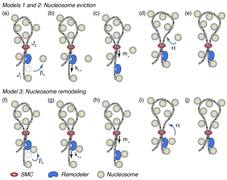
Figure 1: Loop extrusion via a composite LEF, comprising an SMC complex, which forms a ring around two nucleosome-free sections of DNA, nucleosomes that block SMC translocation, and a remodeling complex which removes nucleosomes in front of the SMC. In our model, a single loop extrusion step starts when the remodeling complex forces a nucleosome from the DNA ahead of the remodeler, thus moving the junction (J1) between nucleosomal DNA and naked DNA one step forward. $\beta_{0}$ is the rate of nucleosome dissociation (a) or remodeling (f) when the remodeler is next to a nucleosome. Next, the remodeler moves into the resultant nucleosome-free region, (b) and (g). $k_{1+}$ is the rate at which the remodeler steps forward, when the remodeler-nucleosome separation is one step. Then, the SMC complex moves into the new nucleosome-free region left behind the remodeler (c) and (h). $m_{+}$ is the rate at which the the SMC steps forward on nucleosome-free DNA. Finally, a nucleosome rebinds behind the SMC complex, moving the second junction (J2) between nucleosomal DNA and naked DNA one step forward, and so preventing the SMC from subsequently backtracking. $\alpha$ is the rate of nucleosome rebinding (d) or re-formation (i). After these four sub-steps, the LEF configuration is the same as before the first step, but the loop is one step larger, (e) and (j). The top row (a-e) illustrates a hypothetical scenario (models 1 and 2) in which the displaced nucleosome is in solution before rebinding DNA behind the SMC. The bottom row (f-j) illustrates an alternative “remodeled-nucleosome” scenario (model 3) in which the displaced nucleosome remains associated with the remodeling complex before rebinding DNA behind the SMC.

The notion that nucleosomes might actually represent a barrier for SMC translocation and therefore loop extrusion is suggested by measurements that reveal that cohesin motions on nucleosomal DNA are much reduced compared to those on naked DNA [19]. Further supporting the hypothesis that nucleosomes hinder SMC-driven loop extrusion are several studies indicating that cohesin translocation requires transcription-coupled nucleosome remodeling [20, 21, 22, 23, 24]. In particular, Ref. [24] demonstrates that cohesin, recruited to one genomic location by a cohesin loading complex, is relocated to another by RNA polymerase (Pol II) during transcription. Finally, Ref.  [25] found that presence of nucleosomes in Xenopus laevis egg extract prevented DNA exposed to the extract from looping and compaction.

In this paper, motivated by the possibility that nucleosomes block loop extrusion by SMCs, we introduce and characterize theoretically a composite loop extrusion factor (composite LEF) model that realizes chromatin loop extrusion. Fig. 1 is a cartoon representation of this model. As illustrated in the figure, in addition to an SMC complex that encircles two threads of DNA, creating a chromatin loop, the model includes a remodeling complex, that removes or relocates nucleosomes as it translocates along chromatin, and nucleosomes, that create a barrier for SMC motion. Both the remodeler and the nucleosomes are essential components of the composite LEF.

We envision that when the ring-like SMC complex is threaded by DNA, it can move along the DNA until it encounters a nucleosome, which blocks its motion. We hypothesize that the SMC’s ATPase activity does not exert enough force to move a nucleosome, even though it may give rise to directional loop extrusion on naked DNA. Without nucleosome remodeling, therefore, an SMC complex remains trapped by its surrounding nucleosomes at a more-or-less fixed genomic location. Directional loop extrusion is enabled by SMC motion along the nucleosome-free thread of DNA, that is created in the wake of the remodeling complex, and is maintained by the SMC being held close to the remodeling complex by the ratcheting action of nucleosomes re-locating to behind the SMC. The composite LEF, illustrated in Fig. 1, extrudes the right-hand thread of the chromatin loop, embraced by its constituent SMC complex. The left-hand thread of the loop remains encircled by the SMC at a fixed genomic location, with the SMC trapped by its surrounding nucleosomes. In our model, two-sided loop extrusion would require a remodeler on each thread. The model is agnostic concerning the specific identity of the remodeler, except that it must be able to displace nucleosomes or alter their configuration in a manner that allows the SMC to subsequently pass them by. The top row of Fig. 1 illustrates a hypothetical process, in which the displaced nucleosome unbinds from ahead of the remodeler, before the same or a different nucleosome subsequently rebinds behind the SMC. The bottom row illustrates an alternative version of the model, in which the displaced nucleosome remains associated with the LEF in a transient, “remodeled” configuration, that is permissive to loop extrusion.

This paper is organized as follows. In Sec. II, we calculate the velocities of one-sided loop extrusion for three, slightly different versions of the composite LEF model. In fact, differences among the loop extrusion velocities of the different models are small. In Sec. III, we examine the results of Sec. II to elucidate the conditions required for efficient loop extrusion. We also compare the composite LEF’s loop extrusion velocity to the velocities of the remodeler and the SMC, each translocating alone on chromatin. For a broad range of parameter values, we find that the model’s component factors can indeed be sensibly identified as a composite LEF, that can extrude chromatin loops at a velocity that is comparable to that of isolated remodeler translocation on chromatin, and much faster than loop extrusion by an isolated SMC, that is blocked by nucleosomes. Finally, in Sec. IV, we conclude.

II Theory

The results presented in this section rely on and were guided by the calculations and ideas presented in Refs. [26, 27, 28], concerning other examples of biological Brownian ratchets. To calculate the loop extrusion velocity, $v$, in terms of the rates of remodeling complex forward ($k_{+}$) and backward ($k_{-}$) stepping on DNA, the rates of SMC forward ($m_{+}$) and backward ($m_{-}$) stepping on DNA, and the rates of nucleosome binding ($\alpha$) and unbinding ($\beta$), etc., we make a number of simplifying assumptions. First, we consider chromatin as a sequence of nucleosome binding sites. Second, we assume that the none of the SMC complex, the remodeling complex, and nucleosomes can occupy the same location, i.e. we assume an infinite hard-core repulsion between these factors, that prevents their overlap. Third, we assume that there are well-defined junctions between bare DNA and nucleosomal DNA in front of the remodeler (junction 1) and behind the SMC loop (junction 2), so that when a remodeler forces a nucleosome from junction 1, subsequently it relocates to junction 2. Finally, we hypothesize that, although SMCs can not push nucleosomes out of their way, the remodeling complex can. Following Refs. [27, 28], we actualize this nucleosome-ejecting activity via a nearest-neighbor repulsive interaction, $\Delta G$, between the remodeling complex and junction 1.

II.1 Model 1

First, we consider a streamlined model (model 1), which assumes that the nucleosome unbinding and re-binding rates are much faster than the remodeling complex and SMC forward- and backward-stepping rates. Because of this separation of time scales, we can consider that the SMC and remodeler move in a free energy landscape defined by the time-averaged configuration of nucleosomes [26]. Thus, when the remodeling complex and junction 1 are next to each other (zero separation), the free energy is $\Delta G$, corresponding to the nearest-neighbor remodeler-junction repulsive interaction, or, when there are $n$ nucleosome binding sites between the remodeling complex and junction 1, the free energy is $n\Delta g$, corresponding to the free energy of $n$ unbound nucleosomes in front of the remodeling complex. A straightforward equilibrium statistical mechanical calculation then informs us that the probability that the remodeling complex and junction 1 are not next to each other is

$$P_{1}=\frac{1}{1+e^{\frac{\Delta g-\Delta G}{k_{B}T}}-e^{-\frac{\Delta G}{k_{B}T}}}.$$ (1)

Similarly, the probability that the SMC and junction 2 are not next to each other is

$$P_{2}=e^{-\frac{\Delta g}{k_{B}T}},$$ (2)

because we assume there is not a SMC-nucleosome nearest-neighbor interaction, beyond the requirement that they not be at the same location.

The principle of detailed balance informs us that the ratio of forward and backward transition rates are given by a Boltzmann factor. Therefore, when the the remodeling complex and junction 1 are not next to each other, we expect

$$\frac{k_{+}}{k_{-}}=e^{-\frac{\Delta G_{R}}{k_{B}T}},$$ (3)

where $\Delta G_{R}$ is the free energy change involved in moving the remodeler one step forward. However, when the remodeling complex and junction 1 are next to each other, this ratio of rates is modified, because of the nucleosome-remodeling complex repulsion:

$$\frac{k_{1+}}{k_{0-}}=e^{-\frac{\Delta G}{k_{B}T}}\frac{k_{+}}{k_{-}},$$ (4)

where $k_{1+}$ is the remodeling complex forward stepping rate, when the remodeler-junction 1 separation is one step, and $k_{0-}$ is the remodeling complex backward stepping rate when the remodeler-junction 1 separation is zero. As discussed in detail in Refs. [27, 28], to satisfy Equation (4), in general, we can write

$$k_{1+}=e^{-\frac{\Delta Gf}{k_{B}T}}k_{+},$$ (5)

$$k_{0-}=e^{\frac{\Delta G(1-f)}{k_{B}T}}k_{-},$$ (6)

where $0<f<1$ [27, 28]. However, as discussed in detail in Refs.  [27] and [28] in an analogous context, the choice $f=0$ maximizes the composite LEF velocity. Therefore, we pick $f=0$, so that

$$k_{1+}=k_{+}$$ (7)

and

$$k_{0-}=e^{\frac{\Delta G}{k_{B}T}}k_{-},$$ (8)

which satisfy Equation (4). Then, the mean velocity of the remodeling complex may be written

$$v_{R} =bk_{+}P_{1}-bk_{-}P_{3}P_{1}-bk_{-}e^{\frac{\Delta G}{k_{B}T}}P_{3}(1-P_{1})$$ (9)

where $P_{3}$ is the probability that the remodeling complex and the SMC are not next to each other, and $b$ is the step size along the DNA, taken to be the separation between nucleosomes for simplicity. The first term on the right-hand side of Equation (9) corresponds to stepping forward, which can only happen if the remodeling complex and junction 1 are not next to each other. The second term on the right-hand side of Equation (9) corresponds to stepping backwards in the case that the remodeling complex and junction 1 are not next to each other and the remodeling complex and the SMC complex are not next to each other, in which case the rate of this process is $k_{-}$. The third term on the right-hand side of Equation (9) corresponds to stepping backwards in the case that the remodeling complex and junction 1 are next to each other and the remodeling complex and the SMC complex are not next to each other, in which case the rate of this process is $k_{-}e^{\frac{\Delta G}{k_{B}T}}$, according to Equation (8). Using Equation (1) in Equation (9), we find

$$v_{R} =b\frac{{k_{+}}-k_{-}e^{\frac{\Delta g}{k_{B}T}}P_{3}}{1+e^{\frac{\Delta g-\Delta G}{k_{B}T}}-e^{-\frac{\Delta G}{k_{B}T}}}.$$ (10)

We can also calculate the diffusivity of the remodeler:

$$D_{R} =\frac{1}{2}\left(b^{2}k_{+}P_{1}+b^{2}k_{-}P_{3}P_{1}+b^{2}k_{-}e^{\frac{\Delta G}{k_{B}T}}P_{3}(1-P_{1})\right)$$ (11)

$$=\frac{1}{2}b^{2}\frac{{k_{+}}+k_{-}e^{\frac{\Delta g}{k_{B}T}}P_{3}}{1+e^{\frac{\Delta g-\Delta G}{k_{B}T}}-e^{-\frac{\Delta G}{k_{B}T}}}.$$

Similar reasoning informs us that the velocity and diffusivity of the SMC complex are

$$v_{S}=b(m_{+}P_{3}-m_{-}P_{2})=b(m_{+}P_{3}-m_{-}e^{-\frac{\Delta g}{k_{B}T}}),$$ (12)

and

$$D_{S}=\frac{1}{2}b^{2}(m_{+}P_{3}+m_{-}e^{-\frac{\Delta g}{k_{B}T}}),$$ (13)

respectively.

Equation (10) shows that the velocity of the remodeling complex, $v_{R}$, decreases with increasing $P_{3}$, while Equation (12) shows that the velocity of the SMC complex, $v_{S}$, increases with increasing $P_{3}$. To realize a composite LEF, $P_{3}$ must take on a value that causes these two velocities to coincide, so that the remodeling complex and the SMC complex translocate together with a common velocity, $v$, given by $v=v_{R}=v_{S}$. Equations (10) and (12) constitute two equations for the two unknowns, $P_{3}$ and $v$. Solving yields

$$P_{3} =\frac{\frac{k_{+}}{k_{-}m_{+}}+(e^{-\frac{\Delta g}{k_{B}T}}-e^{-\frac{\Delta g+\Delta G}{k_{B}T}}+e^{-\frac{\Delta G}{k_{B}T}})\frac{m_{-}}{k_{-}m_{+}}}{\frac{e^{\frac{\Delta g}{k_{B}T}}}{m_{+}}+\frac{1+e^{\frac{\Delta g-\Delta G}{k_{B}T}}-e^{-\frac{\Delta G}{k_{B}T}}}{k_{-}}}$$ (14)

and

$$v =b\frac{\frac{k_{+}}{k_{-}}-\frac{m_{-}}{m_{+}}}{\frac{e^{\frac{\Delta g}{k_{B}T}}}{m_{+}}+\frac{1+e^{\frac{\Delta g-\Delta G}{k_{B}T}}-e^{-\frac{\Delta G}{k_{B}T}}}{k_{-}}}.$$ (15)

Using this value for $P_{3}$, it further follows that

$$D_{R}= b^{2}\frac{k_{+}}{1+e^{\frac{\Delta g-\Delta G}{k_{B}T}}-e^{-\frac{\Delta G}{k_{B}T}}}$$ (16)

$$+\frac{1}{2}b^{2}\frac{\frac{m_{-}}{m_{+}}-\frac{k_{+}}{k_{-}}}{\frac{e^{\frac{\Delta g}{k_{B}T}}}{m_{+}}+\frac{1+e^{\frac{\Delta g-\Delta G}{k_{B}T}}-e^{-\frac{\Delta G}{k_{B}T}}}{k_{-}}}$$

and

$$D_{S}= \frac{1}{2}b^{2}\frac{\frac{k_{+}}{k_{-}}+(e^{-\frac{\Delta g}{k_{B}T}}-e^{-\frac{\Delta g+\Delta G}{k_{B}T}}+e^{-\frac{\Delta G}{k_{B}T}})\frac{m_{-}}{k_{-}}}{\frac{e^{\frac{\Delta g}{k_{B}T}}}{m_{+}}+\frac{1+e^{\frac{\Delta g-\Delta G}{k_{B}T}}-e^{-\frac{\Delta G}{k_{B}T}}}{k_{-}}}$$ (17)

$$+\frac{1}{2}b^{2}e^{-\frac{\Delta g}{k_{B}T}}m_{-}.$$

Figure 2: Three example composite LEF trajectories from model 2 simulations. In each case, the positions versus time of the nucleosome junctions are shown gray, the remodeling complex is shown blue, and the SMC complex is shown red. When tracking together, each such group of four traces constitutes a composite LEF. The model parameters are $k_{+}=0.05$ per time step, $k_{-}=5\times 10^{-7}$ per time step, $m_{+}=m_{-}=0.3$ per time step, $\Delta G=18.0k_{B}T$, $\alpha=1$ per time step, and $\beta-\alpha e^{\frac{-\Delta g}{k_{B}T}}$ for all three composite LEFs, but $\Delta g=18.0k_{B}T$ for the bottom group of traces, $\Delta g=9.0k_{B}T$ for the middle group of traces, and $\Delta g=0.5k_{B}T$ for the top group of traces. The cyan, green, and magenta lines each have a slope given by the theoretical composite LEF velocity for the parameters of each simulation.

II.2 Model 2

At the cost of a little complication, it is possible to calculate the composite LEF velocity, even when the nucleosome binding ($\alpha$) and unbinding ($\beta$) rates are not much larger than $k_{+}$, $k_{-}$, $m_{+}$, and $m_{-}$. This model (model 2) is preferable a priori because we expect the nucleosome unbinding rate, $\beta$, to be small. In fact, the results obtained with model 2 are very similar to those obtained with model 1.

Similar to the remodeling complex forward- and backward-stepping rates, when the remodeling complex and junction 1 are adjacent, the nucleosome binding and unbinding rates are modified as follows:

$$\frac{\alpha_{1}}{\beta_{0}}=e^{-\frac{\Delta G}{k_{B}T}}\frac{\alpha}{\beta},$$ (18)

where $\alpha_{1}$ is the nucleosome binding rate when the remodeler-junction 1 separation is one step, and $\beta_{0}$ is the nucleosome unbinding rate when the remodeling complex and junction 1 are adjacent (separation 0). To satisfy Equation (18), we can write

$$\alpha_{1}=e^{-\frac{\Delta Gf}{k_{B}T}}\alpha,$$ (19)

and

$$\beta_{0}=e^{\frac{\Delta G(1-f)}{k_{B}T}}\beta,$$ (20)

which stand alongside Equations (7) and (8). As above, we again choose $f=0$, so that

$$\alpha_{1}=\alpha$$ (21)

and

$$\beta_{0}=e^{\frac{\Delta G}{k_{B}T}}\beta.$$ (22)

To proceed in this case, we first write down the mean velocity of junction 1:

$$v_{J1} =b(\beta-\alpha)P_{1}+b\beta e^{\frac{\Delta G}{k_{B}T}}(1-P_{1}),$$ (23)

where $P_{1}$ is the probability that the remodeling complex and junction 1 are not next to each other and $b$ is the step size. Similarly, we can also write down the mean velocity of the remodeling complex:

$$v_{R}=b(k_{+}-k_{-}P_{3})P_{1}-bk_{-}e^{\frac{\Delta G}{k_{B}T}}(1-P_{1})P_{3},$$ (24)

where $P_{3}$ is the probability that the remodeling complex and the SMC complex are not adjacent to each other. Next, we write down the velocity of the SMC complex:

$$v_{S}=b(m_{+}P_{3}-m_{-}P_{2}),$$ (25)

where $P_{2}$ is the probability that the SMC complex and the junction between bare DNA and nucleosomal DNA behind the SMC complex, namely junction 2, are not adjacent to each other. Finally, we can write down the mean velocity of junction 2:

$$v_{J2}=b(\alpha P_{2}-\beta).$$ (26)

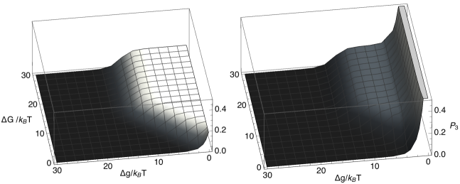
Figure 3: Probability, $P_{3}$, that the remodeling complex and the SMC complex involved in a composite LEF are not adjacent to each other, plotted versus $\Delta G/(k_{B}T)$ and $\Delta g/(k_{B}T)$, according to model 1 [Equation (14)] for $k_{+}=0.05$  per time step, $k_{-}=5.0\times 10^{-7}$ per time step, $m_{+}=0.3$ per time step, and $m_{-}=0.0003$ per time step (left) or $m_{-}=0.3$ per time step (right).

For the composite LEF to translocate as a single entity, it is necessary for each of its component parts to translocate with a common velocity, $v$, where

$$v=v_{J1}=v_{R}=v_{S}=v_{J2}.$$ (27)

Solving Equations (23) through (27) for the four unknowns, namely $v$, and the probabilities, $P_{1}$, $P_{3}$, and $P_{2}$, yields the values of these quantities. To this end, first we solve Equations (23) and (24), assuming that junction 1 and the remodeling complex have a common velocity ($v_{1}$) with the result that

$$v_{1}=b\frac{(\frac{k_{+}}{k_{-}}-\frac{\alpha}{\beta}P_{3})}{(1-e^{-\frac{\Delta G}{k_{B}T}})(\frac{1}{k_{-}}+\frac{P_{3}}{\beta})+\frac{\alpha+k_{+}}{\beta k_{-}}e^{-\frac{\Delta G}{k_{B}T}}}.$$ (28)

Next, we solve Equations (25) and (26), assuming that the SMC complex and junction 2 have a common velocity ($v_{2}$). In this case, we find

$$v_{2}=b\frac{\frac{m_{+}P_{3}}{m_{-}}-\frac{\beta}{\alpha}}{\frac{1}{m_{-}}+\frac{1}{\alpha}}$$ (29)

for the SMC-junction 2 velocity. For these two pairs to translocate together, manifesting a four component, composite LEF, it is necessary that they share a common velocity, $v$, given by $v=v_{1}=v_{2}$. Setting Equation (28) equal to Equation (29) and solving for $P_{3}$, we find

$$P_{3}= \frac{1}{2m_{+}(1-e^{-\frac{\Delta G}{k_{B}T}})}\left(-\alpha-m_{-}-\frac{m_{+}}{k_{-}}(\alpha+k_{+})e^{-\frac{\Delta G}{k_{B}T}}+(\frac{\beta m_{-}}{\alpha}-\frac{\beta m_{+}}{k_{+}})(1-e^{-\frac{\Delta G}{k_{B}T}})\right)$$

$$+\frac{\beta m_{-}}{2m_{+}(1-e^{-\frac{\Delta G}{k_{B}T}})}\sqrt{\begin{aligned} \frac{4m_{+}}{\beta m_{-}}(1-e^{-\frac{\Delta G}{k_{B}T}})(\frac{k_{+}}{\alpha k_{-}}+\frac{k_{+}}{k_{-}m_{-}}+\frac{\beta}{\alpha k_{-}}(1-e^{-\frac{\Delta G}{k_{B}T}})+(\frac{k_{+}}{\alpha k_{-}}+\frac{1}{k_{-}})e^{-\frac{\Delta G}{k_{B}T}})\\ +\left(\frac{1}{\beta}+\frac{\alpha}{\beta m_{-}}+(\frac{\alpha m_{+}}{\beta k_{-}m_{-}}+\frac{k_{+}m_{+}}{\beta k_{-}m_{-}})e^{-\frac{\Delta G}{k_{B}T}}+(\frac{m_{+}}{k_{-}m_{-}}-\frac{1}{\alpha})(1-e^{-\frac{\Delta G}{k_{B}T}})\right)^{2}.\end{aligned}}$$ (30)

The velocity of the composite LEF can be calculated by substituting Equation (30) into Equation (29).

We also carried out a series of Gillespie simulations [29] of model 2 for several values of $\frac{\Delta g}{k_{B}T}$. Fig. 2 shows the position versus time for three example simulations, each carried out for a different value of $\frac{\Delta g}{k_{B}T}$. For each of these LEFs, the gray traces represent the positions of the junctions between nucleosomal DNA and naked DNA, the blue trace represents the position of the remodeling complex, and the red trace represents the position of the SMC complex. The mean position of the bottom LEF, which corresponds to $\frac{\Delta g}{k_{B}T}=18$, remains essentially fixed over the period of the simulation, implying a very small LEF velocity. In addition, in this case, the remodeler and the SMC remain next to each other throughout the trajectory, implying a very small value of $P_{3}$. By contrast, the mean position of the middle LEF ($\frac{\Delta g}{k_{B}T}=8$) increases more-or-less linearly in time with the remodeler and the SMC both stepping forward and frequently moving out of contact. Thus, in this case, the LEF shows a significant velocity and an intermediate value of $P_{3}$. Finally, although the velocity of the top LEF ($\frac{\Delta g}{k_{B}T}=0.5$) is very similar to that of the middle LEF, the top LEF shows many fewer remodeler-SMC contacts than the middle LEF, corresponding to a significantly larger value of $P_{3}$. The cyan, green, and magenta lines in Fig. 2 have slopes given by the corresponding model-2 composite LEF velocities, – calculated by substituting Equation (30) into Equation (29) – revealing good agreement between theory and simulation.

II.3 Model 3

Model 3 supposes that the probability of complete nucleosome unbinding into solution is negligible, but that there exists a ”remodeled” configuration, in which the nucleosome is both associated with the remodeler and also sufficiently displaced to allow the remodeler to step forward (bottom row of Fig. 1). In this model, we interpret $\Delta g$ to be the free energy of the remodeled configuration. For simplicity, we also assume a separation of time scales with remodeling occurring much faster than translocation. Then, the probability that the remodeling complex and junction 1 are not next to each other is

$$P_{1}=\frac{1}{1+e^{\frac{\Delta g-\Delta G}{k_{B}T}}}=\frac{1}{1+(1+e^{\frac{\Delta g}{k_{B}T}})e^{\frac{\Delta G}{k_{B}T}}-e^{\frac{\Delta G}{k_{B}T}}},$$ (31)

while the probability that the SMC and junction 2 are not next to each other is

$$P_{2}=\frac{1}{1+e^{\frac{\Delta g}{k_{B}T}}}.$$ (32)

Equations (31) and (32) replace model 1’s Equations (1) and (2), respectively. However, Equations (9) and (12) are unchanged for model 3. It is apparent therefore that we may write down the model-3 results for $P_{3}$ and $v$ by replacing $e^{\frac{\Delta g}{k_{B}T}}$ in corresponding results for model 1 by $e^{\frac{\Delta g}{k_{B}T}}+1$. Thus, for model 3, we find

$$P_{3} =\frac{\frac{k_{+}}{k_{-}m_{+}}+(\frac{1-e^{-\frac{\Delta G}{k_{B}T}}}{1+e^{\frac{\Delta g}{k_{B}T}}}+e^{-\frac{\Delta G}{k_{B}T}})\frac{m_{-}}{k_{-}m_{+}}}{\frac{1+e^{\frac{\Delta g}{k_{B}T}}}{m_{+}}+\frac{1+e^{\frac{\Delta g-\Delta G}{k_{B}T}}}{k_{-}}}$$ (33)

and

$$v =b\frac{\frac{k_{+}}{k_{-}}-\frac{m_{-}}{m_{+}}}{\frac{1+e^{\frac{\Delta g}{k_{B}T}}}{m_{+}}+\frac{1+e^{\frac{\Delta g-\Delta G}{k_{B}T}}}{k_{-}}}.$$ (34)

III Discussion

To realize a composite LEF, junction 1 and the remodeler, on the one hand, must not outrun the SMC and junction 2, on the other. This requirement may be expressed mathematically by insisting that the probability, $P_{3}$, that the remodeling complex and the SMC are not next to each other, must be less than 1. Otherwise, for $P_{3}=1$, the remodeler and SMC do not come into contact, and we may infer that the remodeler has outpaced the SMC. Fig. 3 plots $P_{3}$, according to model 1, as a function of $\frac{\Delta G}{k_{B}T}$ and $\frac{\Delta g}{k_{B}T}$. For the parameter values, used in the left-hand panel, we see that $P_{3}$ is everywhere less than 1, consistent with the existence of a composite LEF throughout the region illustrated. In fact, $P_{3}$ takes on a relatively large plateau value for

$$\Delta G>\Delta g$$ (35)

and

$$m_{+}>e^{\frac{\Delta g}{k_{B}T}}k_{-}.$$ (36)

Elsewhere, $P_{3}$ is small.

For the parameter values used in the right-hand panel of Fig. 3, however, although $P_{3}$ shows a similar plateau at intermediate values of $\frac{\Delta g}{k_{B}T}$, as $\frac{\Delta g}{k_{B}T}$ decreases to near zero, $P_{3}$ increases rapidly to unity, and according to Equation (14), would unphysically exceed unity for small enough $\frac{\Delta g}{k_{B}T}$. This circumstance arises when even $P_{3}=1$ is not sufficient to satisfy $v_{R}=v_{S}$. When the remodeling complex and junction 1 outrun the SMC and junction 2 – i.e. when $v_{R}>v_{S}$ – the premise of a composite LEF, upon which Equations (14) and (15) are based, can no longer hold. Thus, to achieve a composite LEF, we must have that $v_{R}\leq v_{S}$ for $P_{3}=1$. This condition requires that the model parameter values must satisfy

$$m_{+}-m_{-}e^{-\frac{\Delta g}{k_{B}T}}>\frac{{k_{+}}-k_{-}e^{\frac{\Delta g}{k_{B}T}}}{1+e^{\frac{\Delta g-\Delta G}{k_{B}T}}-e^{-\frac{\Delta G}{k_{B}T}}}.$$ (37)

This condition is violated at small $\Delta g$ for the parameters used in the right-hand panel of Fig. 3. For $k_{+}\gg k_{-}e^{\frac{\Delta g}{k_{B}T}}$ and $m_{+}\gg m_{-}e^{-\frac{\Delta g}{k_{B}T}}$, the condition for a composite LEF to exist becomes simply $m_{+}>k_{+}$, namely the forward stepping rate of the SMC on naked DNA should be larger than the forward stepping rate of the remodeler on naked DNA.

To further elucidate the composite LEF’s behavior as $P_{3}$ increases, we turned to Gillespie simulations of the sort illustrated in Fig. 2. The points in Fig. 4 show the simulated results for both $P_{3}$ itself (top panel) and the remodeler-SMC separation (bottom panel), plotted versus $\frac{\Delta g}{k_{B}T}$. The solid line in the top panel corresponds to Equation (30), demonstrating excellent quantitative agreement between theory and simulation for $P_{3}$. For the parameters of Fig. 4, as $\frac{\Delta g}{k_{B}T}$ decreases below about 3, $P_{3}$ increases from its plateau value, eventually reaching unity at $\frac{\Delta g}{k_{B}T}\simeq 0.2$. Thus, in this case, for $\frac{\Delta g}{k_{B}T}<0.2$, a composite LEF does not exist.

It is apparent from the bottom panel of Fig. 4, that the remodeler-SMC separation matches $P_{3}$ for $\frac{\Delta g}{k_{B}T}\geq 3$. This result obtains because, for $\frac{\Delta g}{k_{B}T}\geq 3$, the overwhelmingly prevalent remodeler-SMC separations are 0 and 1, so that the calculation of $P_{3}$ and the calculation of the mean remodeler-SMC separation are effectively the same calculation in this regime. However, as $\frac{\Delta g}{k_{B}T}$ decreases below 3, the mean remodeler-SMC separation rapidly increases beyond $P_{3}$, as larger remodeler-SMC separations than 1 become prevalent, as may seen for the top LEF in Fig. 2, which corresponds to $\frac{\Delta g}{k_{B}T}=0.5$. The mean remodeler-SMC separation reaches 1 for $\frac{\Delta g}{k_{B}T}\lesssim 1.3$ and rapidly increases as $\frac{\Delta g}{k_{B}T}$ decreases further.

A key assumption of our theory is that displaced nucleosomes rebind only at junctions between nucleosomal DNA and naked DNA. However, when the model predicts a relatively large region of naked DNA between the remodeler and the SMC, into which a nucleosome could easily fit, this assumption seems likely to be inappropriate and the model no longer self-consistent, in turn suggesting that the condition specified by Equation (37) may be too permissive. However, further investigation of this question lies beyond the simple model described here.

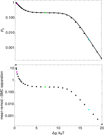
Figure 4: The probability, $P_{3}$, that the remodeler and SMC are not next to each other (top) and the mean remodeler-SMC separation (bottom), plotted versus nucleosome binding energy, $\frac{\Delta g}{k_{B}T}$. The circles correspond to results determined from model-2 Gillepsie simulations, each containing $2^{20}$ transitions. The solid line corresponds to Equation (30). The parameter values used were: $k_{+}=0.05$ per time step, $k_{-}=5\times 10^{-7}$ per time step, $m_{+}=m_{-}=0.3$ per time step, $\Delta G=18.0k_{B}T$, $\alpha=1$ per time step, and $\beta=\alpha e^{-\frac{\Delta g}{k_{B}T}}$. These parameters correspond to those for Fig. 2. The cyan, green, and magenta points at $\frac{\Delta g}{k_{B}T}=0.5$, $8.0$, and $18$, respectively, correspond to the bottom, middle, and top traces of Fig. 2.

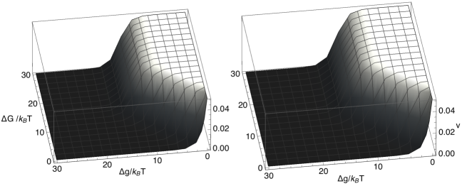
Figure 5: Mean velocity, $v$, of a composite LEF plotted versus $\frac{\Delta G}{k_{B}T}$ and $\frac{\Delta g}{k_{B}T}$, according to Equation (15) for $k_{+}=0.05$ per time step, $k_{-}=5.0\times 10^{-7}$ per time step, $m_{+}=0.3$ per time step, and $m_{-}=0.0003$ per time step (left) or $m_{-}=0.3$ per time step (right).

Fig. 5 plots the model-1 LEF velocity, corresponding to the probabilities displayed in Fig. 3, showing that $v$ achieves a relatively large plateau value when the conditions,

$$\Delta G>\Delta g$$ (38)

and

$$m_{+}>e^{\frac{\Delta g}{k_{B}T}}k_{-},$$ (39)

are both satisfied. Equation (38) informs us that to achieve rapid composite LEF translocation, a large repulsive nucleosome-remodeling complex interaction ($\Delta G$) is necessary, that overcomes the nucleosome binding free energy ($\Delta g$). We might have expected that rapid composite LEF translocation would also require that the rate at which the SMC complex steps forward into a gap between the SMC complex and the remodeling complex must exceed the rate at which the remodeling complex steps backwards into that same gap, which is $e^{\frac{\Delta G}{k_{B}T}}k_{-}$, i.e. we might have expected that $m_{+}>e^{\frac{\Delta G}{k_{B}T}}k_{-}$. However, because of Equation (38), Equation (39) is actually a weaker condition on $m_{+}$ than this expectation.

Fig. 6 illustrates the model 1 diffusivities of the remodeling complex and the SMC complex. Each diffusivity specifies the corresponding factor’s positional fluctuations, about the mean displacement, determined by the velocity. The diffusivities also show relatively large plateau values when Equations (38) and (39) are satisfied. Surprisingly, the diffusivity of the remodeling complex also shows a second plateau with an even higher plateau value for $\Delta G>\Delta g$ and $m_{+}<e^{\frac{\Delta g}{k_{B}T}}k_{-}$, where the corresponding composite LEF velocity is small.

When all of Equations (37), (38) and (39) are simultaneously satisfied, the plateau values of the the probability that the remodeling complex and the SMC complex are not next to each other, the LEF velocity, and the two diffusivities are given approximately by

$$P_{3}\simeq\frac{k_{+}}{m_{+}},$$ (40)

$$v\simeq bk_{-}(\frac{k_{+}}{k_{-}}-\frac{m_{-}}{m_{+}}),$$ (41)

$$D_{R}\simeq\frac{1}{2}b^{2}k_{-}(\frac{k_{+}}{k_{-}}+\frac{m_{-}}{m_{+}}),$$ (42)

and

$$D_{S}\simeq\frac{1}{2}b^{2}k_{+},$$ (43)

respectively. The plateau value of the composite LEF’s loop extrusion velocity is independent of $\Delta g$. This result is possible (although not required – see below) because a loop extrusion step does not lead to a net change in the nucleosome configuration.

Fig. 5 shows that the LEF velocity is inevitably small for small $\Delta G$. For $\Delta G=0$, corresponding to solely hard-core repulsions between the remodeler and a nucleosome – what could be termed a “passive” composite LEF, in analogy to the passive helicase, discussed for example in Ref. [28] – Equation (15) becomes

$$v=be^{-\frac{\Delta g}{k_{B}T}}\frac{\frac{k_{+}}{k_{-}}-\frac{m_{-}}{m_{+}}}{\frac{1}{m_{+}}+\frac{1}{k_{-}}}.$$ (44)

In this case, the composite LEF velocity decreases exponentially with the free energy of nucleosome unbinding, $\Delta g$. Since $\Delta g$ is several tens of $k_{B}T$, we do not expect this limit to be feasible for effective loop extrusion. Although Equation (44) corresponds to $f=0$ and $\Delta G=0$, it may be shown that it also gives the LEF velocity for $f=1$ in the large-$\Delta G$ limit. This is because for $f=1$, large $\Delta G$ effectively creates a hard wall for the remodeler, albeit located one step away from the nucleosome, recapitulating the situation considered for $f=0$ and $\Delta G=0$.

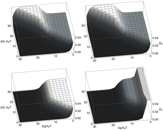
Figure 6: Diffusivities, $D_{R}$ (top row) and $D_{S}$ (bottom row) of the remodeling complex and the SMC complex, respectively, plotted versus $\Delta G/(k_{B}T)$ and $\Delta g/(k_{B}T)$, according to model 1 [Equations (16) and (17)] for $k_{+}=0.05$ per time step, $k_{-}=5.0\times 10^{-7}$ per time step, $m_{+}=0.3$ per time step, and $m_{-}=0.0003$ per time step (left column) or $m_{-}=0.3$ per time step (right column).

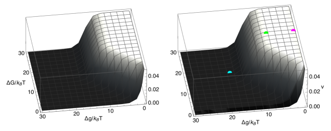
Figure 7: Mean velocity, $v$, of a composite LEF, plotted versus $\Delta G/(k_{B}T)$ and $\Delta g/(k_{B}T)$ for model 1 (left) and model 2 (right) for $k_{+}=0.05$ per time step, $k_{-}=5.0\times 10^{-7}$ per time step, $m_{+}=0.3$ per time step, $m_{-}=0.0003$ per time step, and (for model 2) $\alpha=1$ per time step. The cyan, green, and magenta points on the model-2 curve correspond to the theoretical mean velocities of the composite LEFs whose positions versus time are shown in Fig. 2.

In comparison to Equation (15), the velocity of a lonely remodeling complex, translocating on nucleosomal DNA, unaccompanied by an SMC complex, is

$$v_{R} =bk_{+}P_{1}-bk_{-}e^{-\frac{\Delta g}{k_{B}T}}(P_{1}+(1-P_{1})e^{\frac{\Delta G}{k_{B}T}})$$ (45)

$$=b\frac{k_{+}-k_{-}}{1+e^{\frac{\Delta g-\Delta G}{k_{B}T}}-e^{-\frac{\Delta G}{k_{B}T}}},$$

which may be straightforwardly obtained from Equation (10) by replacing $P_{3}$ with $e^{-\frac{\Delta g}{k_{B}T}}$, which is the probability that there is a gap between the remodeler and junction 2. The velocity of such a lonely remodeling complex is relatively large for $\Delta G>\Delta g$ and is small otherwise. Thus, as seems intuitive, for efficient remodeler translocation on chromatin the remodeler-nucleosome repulsive free energy, $\Delta G$ must exceed the free energy required for nucleosome unbinding, $\Delta g$. In the large-$\Delta G$ limit, the remodeler velocity realizes a plateau value of

$$v_{R}=b(k_{+}-k_{-})=bk_{-}(\frac{k_{+}}{k_{-}}-1),$$ (46)

so that the plateau velocity of a composite LEF exceeds (is less than) [equals] that of a lonely remodeling complex for $m_{+}>m_{-}$ ($m_{+}<m_{-}$) [$m_{+}=m_{-}$].

We can also straightforwardly calculate the velocity of the SMC complex on nucleosomal DNA in the absence of the remodeling complex with the result that

$$v_{S}=be^{-\frac{\Delta g}{k_{B}T}}(m_{+}-m_{-}).$$ (47)

Equation (47) informs us that, on nucleosomal DNA, the velocity of loop extrusion by an isolated SMC complex, which by assumption does not have its own nucleosome remodeling activity, is suppressed by a factor $e^{-\frac{\Delta g}{k_{B}T}}$ compared to the velocity of its loop extrusion on nucleosome-free DNA, which is $b(m_{+}-m_{-})$. Since $e^{-\frac{\Delta g}{k_{B}T}}$ is tiny, the velocity of the SMC without the remodeling complex is correspondingly tiny, even for $m_{+}\gg m_{-}$, emphasizing that the remodeling complex is essential for significant loop extrusion in the chromatin context.

Equation (15) informs us that the composite LEF’s directionality depends only on $\frac{k_{+}}{k_{-}}-\frac{m_{-}}{m_{+}}$. Since we can expect that $\frac{k_{+}}{k_{-}}=e^{-\frac{\Delta G_{R}}{k_{B}T}}$ and $\frac{m_{+}}{m_{-}}=e^{-\frac{\Delta G_{S}}{k_{B}T}}$, where $\Delta G_{R}$ is the free energy change associated with the remodeling complex stepping forward and $\Delta G_{S}$ is the free energy change, associated with the SMC complex stepping forward, it is clear that the composite LEF proceeds forward, only provided $\Delta G_{R}+\Delta G_{S}<0$. This outcome reflects the Second Law of Thermodynamics, expressed in the form that a chemical reaction proceeds forward only if the corresponding change in free energy is negative. In comparison, Equation (45) informs us that a lonely remodeling complex proceeds forwards if $\Delta G_{R}<0$.

Shown in Fig. 7 is a comparison between the LEF velocity for model 2 and the LEF velocity for model 1. Model 2 reproduces both the region in the $\Delta G$-$\Delta g$ plane where the composite LEF velocity is large and the plateau value of the LEF velocity within that region [Equation (41)]. The cyan, green, and magenta points on the model-2 curve in Fig. 7 correspond to the free energy settings and theoretical mean velocities of the composite LEFs, whose simulated positions versus time are shown in Fig. 2. Both the top group of traces and the middle group of traces in Figure 2 fall within the plateau region of the velocity, which explains why their velocities are very similar. However, while the middle LEF does fall within the plateau region of $P_{3}$, the top composite LEF exhibits a significantly large value of $P_{3}$ and a correspondingly larger spatial extent.

The conceptually simplest versions of the composite LEF model (models 1 and 2) envision that the remodeler ejects a nucleosome from the DNA ahead of the remodeler, and that the nucleosome subsequently rebinds behind the SMC. Alternatively, model 3 hypothesizes an intermediate, “remodeled” state in which the displaced nucleosome remains associated with the LEF, eventually to relocate behind SMC. This picture is reminiscent of the scenario envisioned in Ref. [30], which demonstrated experimentally that RNA polymerase could pass a nucleosome without causing nucleosome dissociation. Nonetheless, for $e^{\frac{\Delta g}{k_{B}T}}\gg 1$, the predictions of all three models are indistinguishable. The interpretation of $\Delta g$ is different for models 1 and 2, on the one hand, and model 3 on the other. For models 1 and 2, $\Delta g$ is the nucleosome binding free energy, which is several tens of $k_{B}T$. For model 3, $\Delta g$ is the free energy of the remodeled configuration, relative to the free energy of a bound nucleosome, which we may expect to be smaller than the free energy required to nucleosome unbinding (models 1 and 2). However, as noted above, the plateau value of the composite LEF’s loop extrusion velocity is independent of $\Delta g$ for all of the models.

IV Conclusions

A key result of this paper is that even if nucleosomes block SMC translocation, efficient loop extrusion remains possible on chromatinized DNA via a LEF, that is a composite entity involving a remodeler and nucleosomes, as well as an SMC complex. Thus, the possibility that nucleosomes may block SMC translocation and loop extrusion on chromatin is not a reason to rule out the loop extrusion factor model of genome organization.

We have shown that, for a wide range of possible parameter values, such a composite LEF exists and can give rise to loop extrusion with a velocity, that is comparable to the remodeler’s translocation velocity on chromatin, but is much larger than the velocity of a SMC complex that is blocked by nucleosomes. Although we have focused on one-sided loop extrusion, two-sided loop extrusion simply requires two remodelers, one for each chromatin strand threading the SMC.

The composite LEF model is agnostic concerning whether the SMC complex shows ATP-dependent translocase activity ($m_{+}\neq m_{-}$) or diffuses ($m_{+}=m_{-}$) on naked DNA. However, Equation 37 specifies the condition for a composite LEF to exist defined by the SMC and the remodeler being in close proximity, while efficient chromatin loop extrusion requires repulsion between the remodeler and the junction between nucleosomal DNA and naked DNA, that is large compared to the nucleosome binding free energy (models 1 and 2) or the remodeled configuration free energy (model 3): $\Delta G>\Delta g$. An additional condition necessary for efficient loop extrusion is $m_{+}>e^{\frac{\Delta g}{k_{B}T}}k_{-}$. Finally, we remark that the composite LEF model, described in this paper, is quite distinct from the models of Refs. [31, 32], which propose loop extrusion occurs without the involvement of a translocase.

- [1] https://bionumbers.hms.harvard.edu.
- Dekker et al. [2002] J. Dekker, K. Rippe, M. Dekker, and N. Kleckner, Capturing chromosome conformation, Science 295, 1306 (2002).
- Dixon et al. [2012] J. R. Dixon, S. Selvaraj, F. Yue, A. Kim, Y. Li, Y. Shen, M. Hu, J. S. Liu, and B. Ren, Topological domains in mammalian genomes identified by analysis of chromatin interactions, Nature 485, 376 (2012).
- Dixon et al. [2016] J. R. Dixon, D. U. Gorkin, and B. Ren, Chromatin domains: The unit of chromosome organization, Mol Cell 62, 668 (2016).
- Sexton et al. [2012] T. Sexton, E. Yaffe, E. Kenigsberg, F. Bantignies, B. Leblanc, M. Hoichman, H. Parrinello, A. Tanay, and G. Cavalli, Three-dimensional folding and functional organization principles of the Drosophila genome, Cell 148, 458 (2012).
- Mizuguchi et al. [2014] T. Mizuguchi, G. Fudenberg, S. Mehta, J. M. Belton, N. Taneja, H. D. Folco, P. FitzGerald, J. Dekker, L. Mirny, J. Barrowman, and S. I. Grewal, Cohesin-dependent globules and heterochromatin shape 3D genome architecture in :s. pombe, Nature 516, 432 (2014).
- Dekker [2014] J. Dekker, Two ways to fold the genome during the cell cycle: Insights obtained with chromosome conformation capture, Epigenetics Chromatin 7, 25 (2014).
- Alipour and Marko [2012] E. Alipour and J. F. Marko, Self-organization of domain structures by DNA-loop-extruding enzymes, Nucleic acids research 40, 11202 (2012).
- Sanborn et al. [2015] A. L. Sanborn, S. S. Rao, S. C. Huang, N. C. Durand, M. H. Huntley, A. I. Jewett, I. D. Bochkov, D. Chinnappan, A. Cutkosky, J. Li, K. P. Geeting, A. Gnirke, A. Melnikov, D. McKenna, E. K. Stamenova, E. S. Lander, and E. L. Aiden, Chromatin extrusion explains key features of loop and domain formation in wild-type and engineered genomes, Proc Natl Acad Sci U S A 112, E6456 (2015).
- Fudenberg et al. [2016] G. Fudenberg, M. Imakaev, C. Lu, A. Goloborodko, N. Abdennur, and L. A. Mirny, Formation of chromosomal domains by loop extrusion, Cell Reports 15, 2038 (2016).
- Nuebler et al. [2018] J. Nuebler, G. Fudenberg, M. Imakaev, N. Abdennur, and L. A. Mirny, Chromatin organization by an interplay of loop extrusion and compartmental segregation, Proc Natl Acad Sci U S A 115, E6697 (2018).
- Goloborodko et al. [2016a] A. Goloborodko, J. F. Marko, and L. A. Mirny, Chromosome compaction by active loop extrusion, Biophysical journal 110, 2162 (2016a).
- Goloborodko et al. [2016b] A. Goloborodko, M. V. Imakaev, J. F. Marko, and L. Mirny, Compaction and segregation of sister chromatids via active loop extrusion, eLife 5, e14864 (2016b).
- Uhlmann [2014] Y. M. . F. Uhlmann, Biochemical reconstitution of topological DNA binding by the cohesin ring, Nature 505, 367 (2014).
- Khoury et al. [2020] A. Khoury, J. Achinger-Kawecka, S. A. Bert, G. C. Smith, H. J. French, P.-L. Luu, T. J. Peters, Q. Du, A. J. Parry, F. Valdes-Mora, P. C. Taberlay, C. Stirzaker, A. L. Statham, and S. J. Clark, Constitutively bound CTCF sites maintain 3D chromatin architecture and long-range epigenetically regulated domains, Nature Communications 11, 54 (2020).
- Ganji et al. [2018] M. Ganji, I. A. Shaltiel, S. Bisht, E. Kim, A. Kalichava, C. H. Haering, and C. Dekker, Real-time imaging of DNA loop extrusion by condensin, Science 360, 102 (2018).
- Kim et al. [2019] Y. Kim, Z. Shi, H. Zhang, I. J. Finkelstein, and H. Yu, Human cohesin compacts DNA by loop extrusion, Science 366, 1345 (2019).
- Kong et al. [2020] M. Kong, E. E. Cutts, D. Pan, F. Beuron, T. Kaliyappan, C. Xue, E. P. Morris, A. Musacchio, A. Vannini, and E. C.Greene, Human condensin I and II drive extensive ATP-dependent compaction of nucleosome-bound DNA, Molecular Cell 79, 99 (2020).
- Stigler et al. [2016] J. Stigler, G. O. Camdere, D. E. Koshland, and E. C. Greene, Single-molecule imaging reveals a collapsed conformational state for DNA-bound cohesin, Cell Rep 15, 988 (2016).
- Dubey and Gartenberg [2007] R. N. Dubey and M. R. Gartenberg, A tDNA establishes cohesion of a neighboring silent chromatin domain, Genes Dev 21, 2150 (2007).
- Glynn et al. [2004] E. F. Glynn, P. C. Megee, H. G. Yu, C. Mistrot, E. Unal, D. E. Koshland, J. L. DeRisi, and J. L. Gerton, Genome-wide mapping of the cohesin complex in the yeast saccharomyces cerevisiae, PLoS Biol 2, E259 (2004).
- Lengronne et al. [2004] A. Lengronne, Y. Katou, S. Mori, S. Yokobayashi, G. P. Kelly, T. Itoh, Y. Watanabe, K. Shirahige, and F. Uhlmann, Cohesin relocation from sites of chromosomal loading to places of convergent transcription, Nature 430, 573 (2004).
- Schmidt et al. [2009] C. K. Schmidt, N. Brookes, and F. Uhlmann, Conserved features of cohesin binding along fission yeast chromosomes, Genome Biol 10, R52 (2009).
- Davidson et al. [2016] I. F. Davidson, D. Goetz, M. P. Zaczek, M. I. Molodtsov, P. J. Huis In ’t Veld, F. Weissmann, G. Litos, D. A. Cisneros, M. Ocampo-Hafalla, R. Ladurner, F. Uhlmann, A. Vaziri, and J. M. Peters, Rapid movement and transcriptional re-localization of human cohesin on DNA, EMBO J 35, 2671 (2016).
- Golfier et al. [2020] S. Golfier, T. Quail, H. Kimura, and J. Brugués, Cohesin and condensin extrude loops in a cell-cycle dependent manner, eLife 9, e53885 (2020).
- Peskin et al. [1993] C. S. Peskin, G. M. Odell, and G. F. Oster, Cellular motions and thermal fluctuations: the Brownian ratchet, Biophys J. 65, 316 (1993).
- Betterton and Jülicher [2003] M. D. Betterton and F. Jülicher, A motor that makes its own track: Helicase unwinding of DNA, Physical Review Letters 91, 258103 (2003).
- Betterton and Jülicher [2005] M. D. Betterton and F. Jülicher, Opening of nucleic-acid double strands by helicases: Active versus passive opening, Phys. Rev. E 71, 011904 (2005).
- Gillespie [1977] D. T. Gillespie, Exact stochastic simulation of coupled chemical reactions, The Journal of Physical Chemistry 81, 2340 (1977).
- Hodges et al. [2009] C. Hodges, L. Bintu, L. Lubkowska, M. Kashlev, and C. Bustamante, Nucleosomal fluctuations govern the transcription dynamics of RNA polymerase II, Science 325, 626 (2009).
- Brackley et al. [2017] C. A. Brackley, J. Johnson, D. Michieletto, A. N. Morozov, M. Nicodemi, P. R. Cook, and D. Marenduzzo, Nonequilibrium chromosome looping via molecular slip links, Physical Review Letters 119, 138101 (2017).
- Maji et al. [2020] A. Maji, R. Padinhateeri, and M. K. Mitra, The accidental ally: Nucleosome barriers can accelerate cohesin-mediated loop formation in chromatin, Biophys. J. 119, 2316 (2020).