Contrastive Explanations for Model Interpretability

Abstract

Contrastive explanations clarify why an event occurred in contrast to another. They are inherently intuitive to humans to both produce and comprehend. We propose a method to produce contrastive explanations in the latent space, via a projection of the input representation, such that only the features that differentiate two potential decisions are captured. Our modification allows model behavior to consider only contrastive reasoning, and uncover which aspects of the input are useful for and against particular decisions. Additionally, for a given input feature, our contrastive explanations can answer for which label, and against which alternative label, is the feature useful. We produce contrastive explanations via both high-level abstract concept attribution and low-level input token/span attribution for two NLP classification benchmarks. Our findings demonstrate the ability of label-contrastive explanations to provide fine-grained interpretability of model decisions.

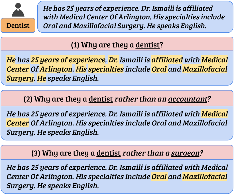
Figure 1: Illustrative example of a biography from BIOS De-Arteaga et al. (2019) with explanations for the occupation label highlighted in yellow. Explanations without an explicit contrast (1) are potentially misaligned with human expectations of what is being explained, making them confusing for human interpretability. Contrastive explanations (2, 3) prune the space of all causal factors to ‘intuitively’ relevant ones, aiding finer-grained understanding, and can vary based on the contrast decision (e.g. accountant, surgeon).

1 Introduction

Explanations in machine learning attempt to uncover the causal factors leading to a model’s decisions. Methods for producing model explanations often seek all causal factors at once—making them difficult to comprehend—or organize the factors via heuristics, such as gradient saliency Simonyan et al. (2013); Li et al. (2016). However, it remains unclear what makes a particular collection of causal factors a good explanation.

Studies in social science establish that human explanations, conversely, are typically “contrastive” Miller (2019): they rely on the causal factors that explain why an event occurred instead of an alternative event Lipton (1990). Such explanations promote easier communication by pruning the space of all causal factors, reducing cognitive load for the explainer and explainee, as illustrated in Figure 1. This reduction is deeply relevant: since explanations of opaque ML and NLP models are approximations of complex statistical processes, humans interpret these decisions subjectively by assuming some contrast decision.

Our work seeks to design explanations that are explicitly contrastive, thereby revealing fine-grained aspects of model decisions, while being more representative of human comprehension (§2). We introduce a novel framework for deriving contrastive explanations applicable to any neural classifier (§3). Our method operates on the input representation space, and produces a latent, contrastive representation. We accomplish this by projecting the latent representations of the input to the space that minimally separates two decisions in the model. We additionally propose a measure of contrastiveness (§3.4) by computing changes to model behavior before and after the projection.

Our experiments consider two well-studied NLP classification benchmarks: MultiNLI (Williams et al., 2018; §4) and BIOS (De-Arteaga et al., 2019; §5). In each, we study explanations in the form of high-level concept features or low-level textual highlights in the input. Our contrastive explanations uncover input features useful for and against particular decisions, and can answer which alternative label was a decision made against; this has potential implications for model debugging. Overall, we find that a contrastive perspective aids fine-grained understanding of model behavior.

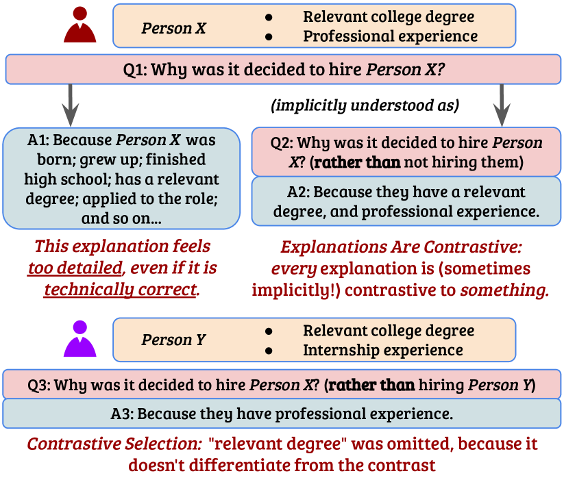
Figure 2: Illustrating contrastive (A2, A3) and non-contrastive (A1) explanations (§2): humans intuitively produce and interpret explanations contrastively.

2 Contrastive Explanations

Explanations can be considered as answers to the question: “why $P$?” where $P$, the fact, is the event to be explained. Consider the question (Q1; Fig. 2):

Why was it decided to hire [Person X]?

The explanation behind decision $P$ (the hiring decision) comprises the causal chain of events that led to $P$; a ‘reasonable’ answer to the question may cite that Person X has relevant degrees or professional experience. However, explaining the complete causal chain (A1; Fig. 2) is both burdensome to the explainer and cognitively demanding to the explainee Hilton and Slugoski (1986); Hesslow (1988). For instance, the hiring event above is caused by Person X’s application for the role—yet a reasonable explainer will likely omit this factor from the explanation for simplicity, thus reducing the cognitive load. But which factors should be omitted, and which should not?

The theory of contrastive explanations provides a solution common in human explanations, which inherently answer the question: “why $P$, rather than $Q$?” Hilton (1988), where $Q$ (the foil) is some alternative event. Therefore, the explanation to the hiring decision might answer (Q2; Fig. 2):

Why was it decided to hire [Person X], rather than not hiring them?

Since the decision not to hire the candidate can also be traced back to the fact that they applied to the role, the explanation can be simplified by omitting this factor (A2; Fig. 2); this illustrates contrastive causal attribution (§3.3) in the explanation process. Similarly, given a different foil (Q3; Fig. 2):

Why was it decided to hire [Person X], rather than hiring [Person Y]?

the explainer might find it unnecessary to include attributes (such as a “relevant college degree”) common to both Person X and Person Y (A3; Fig. 2). For the rest of the paper, we will refer to explanations which are not explicitly contrastive, such as A1 in Fig. 2, as non-contrastive explanations.

Implications for model explanations:

Model explanations can benefit from explicit contrastiveness in two ways. Model decisions are complex and noisy statistical processes—‘complete’ explanations are difficult Jacovi and Goldberg (2020b). Contrastive explanations make model decisions easier to explain by omitting many factors, given the relevant foils. This reduces the burden of the explaining algorithm to interpret and communicate the ‘complete’ reasoning. Additionally, humans tend to inherently, and often implicitly, comprehend (model) explanations contrastively. However, the foil perceived by the explainee may not match the one truly entailed by the explanation (e.g., Kumar et al., 2020); contrastive explanations make the foil explicit, and are therefore easier to understand.

3 Contrastive Explanations Framework

We present our framework for producing contrastive explanations. We describe the preliminaries for our framework (§3.1), and outline an interventionist approach for causal attribution (§3.2). Next, we introduce our projection-based method to produce latent contrastive representations (§3.3) and a measure of the resulting behavioral change (§3.4).

3.1 Preliminaries

Candidate Factor Space:

All causal factors that could possibly lead to the model’s decision. These could include discrete features in the input (textual highlights; Lei et al., 2016; see Fig. 1), abstract input features (concepts; Kim et al., 2017; see Table 4 for an example of gender as a concept), or influential examples in the training set for a prediction Koh and Liang (2017); Han et al. (2020). Once defined, a subset of factors from the candidate factor space can then be causally attributed to the model decision. Our framework is agnostic to the type of factor in the candidate factor space, so long as it is possible to intervene on their presence (§3.2). Our work focuses on textual highlights and concepts.

Event Space:

The union (as a discrete set) of all possible model decision classes. This includes the event we attempt to explain (the fact), i.e. a trained model’s decision, as well all other classes (the foils), considered independently.

3.2 Causal Attribution via Interventions

Given a candidate factor space, we seek to attribute factors with causality over the decision process, i.e. select factors which caused the model’s decision. We adopt an interventionist approach Woodward (2003)—this involves determining causality of a factor by intervening on it, thereby producing a counterfactual. The importance of the intervened factor is determined by change in model behavior under this counterfactual.

Most interventions we consider are amnesic, i.e. use counterfactuals which omit the candidate factors under consideration. Factors in the form of highlights and concepts involve different kinds of interventions. For the former, we simply replace each highlighted token with a ‘mask’ token (§4.2,5.2), and train models where such masked data is in distribution Zintgraf et al. (2017); Kim et al. (2020), i.e. pre-trained masked language models, such as RoBERTa Liu et al. (2019). For conceptual interventions, we employ an amnesic operation to remove a concept from the input representation (§4.1,5.1). Following Elazar et al. (2021), this amnesic operation uses a null-space projection to iteratively remove all linear directions correlated with the concept, until it is not possible to linearly discover the concept information from the latent vector Ravfogel et al. (2020). Training an amnesic probe requires labels indicating presence of the concept for each example ( App. A.1). Where possible, we also employ a conceptual intervention via manually-annotated counterfactuals Kaushik et al. (2020); Gardner et al. (2020) which involve textual modifications to existing data instances (§4.1; Hyp-Negation).

3.3 Contrastive Attribution

While the aforementioned interventions select the causal factors from the candidate factor space for model explanations, we are specifically interested in selecting factors that yield contrastive explanations. Given a space of discovered causal factors, we therefore need an additional intervention to attribute contrastive behavior to a subset of these factors. We propose a method below to produce contrastive explanations in the form of a dense representation of the input in the latent space. This representation is given by a projection operation, such that only the components that distinguish the fact from the foil are preserved.

Formally, let $\mathbf{x}$ be the text input to be classified as one of $K$ output classes $\mathcal{Y}=\{y_{1},...,y_{K}\}$. Consider the model class $f$, which commonly uses an arbitrarily deep neural encoder $\text{{enc}}(\cdot)$ that transforms the input $\mathbf{x}$ into a vector $\mathbf{h}_{\mathbf{x}}\in\mathbb{R}^{d}$. Once encoded, a final linear layer, $\mathbf{W}\in\mathbb{R}^{K\times d}$ can then be applied to the input to yield the logits of the model over the $K$ classes, such that $f(\mathbf{x})=\mathbf{W}\text{{enc}}(\mathbf{x})=\mathbf{W}\mathbf{h}_{\mathbf{x}}$. Let $y^{*}=\operatorname*{arg\,max}_{y\in\mathcal{Y}}f(\mathbf{x})$ be the model prediction (the fact), $y^{\prime}$ be an alternative prediction of interest (the foil), and ${p}:=\text{{softmax}}(\mathbf{W}\mathbf{h}_{\mathbf{x}})$ the normalized model probabilities.

Recall that output of the model, $f(\mathbf{x})=\mathbf{W}\mathbf{h}_{\mathbf{x}}$ is linear in the latent input representation, $\mathbf{h}_{\mathbf{x}}$. Let ${\mathbf{w}_{i}}$ be the row in $\mathbf{W}$ corresponding to class $i$. The logits for classes $y^{\prime},y^{*}$, given by the dot products ${\mathbf{w}_{y^{\prime}}}^{T}\mathbf{h}_{\mathbf{x}}$ and ${\mathbf{w}_{y^{*}}}^{T}\mathbf{h}_{\mathbf{x}}$ respectively, are thus unrelated to any other row in the prediction matrix. These dot products are un-normalized projections of the representation $\mathbf{h}_{\mathbf{x}}$ on the directions ${\mathbf{w}_{y^{*}}},{\mathbf{w}_{y^{\prime}}}\in\mathbb{R}^{d}$. While the representation $\mathbf{h}_{\mathbf{x}}$ can be high-dimensional, only two directions (components) in this high-dimensional space are relevant for each contrastive decision. Furthermore, we are interested in the prediction of one class over the other, as opposed to the logits. Hence, we can replace these two directions with a single contrastive direction ${\mathbf{u}}\in\mathbb{R}^{d}$, by defining ${\mathbf{u}}={\mathbf{w}_{y^{*}}}-{\mathbf{w}_{y^{\prime}}}$.

Given that the model favors $y^{*}$ over $y^{\prime}$, i.e., $p_{y^{*}}>p_{y^{\prime}}$, if and only if ${\mathbf{u}}^{T}\mathbf{h}_{\mathbf{x}}>0$, the projection of $\mathbf{h}_{\mathbf{x}}$ onto ${\mathbf{u}}$ precisely yields the linear direction in $\mathbb{R}^{d}$ which the model uses to differentiate between classes $y^{*}$ and $y^{\prime}$. We refer to the span of the $\mathbf{u}$—that is, the collection of all vectors $\alpha\mathbf{u}$ for a scalar $\alpha$—as the contrastive space for $y^{*}$ and $y^{\prime}$. We define the contrastive transformation $C(\mathbf{h}_{\mathbf{x}})_{y^{\prime},y^{*}}$ to be the orthogonal projection onto this subspace:

$$C(\mathbf{h}_{\mathbf{x}})_{y^{\prime},y^{*}}:= \frac{\mathbf{u}\mathbf{u}^{T}}{\mathbf{u}^{T}\mathbf{u}}\mathbf{h}_{\mathbf{x}}=\mathbf{P}_{\mathbf{u}}\mathbf{h}_{\mathbf{x}},$$ (1)

where $\mathbf{P}_{\mathbf{u}}:=\frac{\mathbf{u}\mathbf{u}^{T}}{\mathbf{u}^{T}\mathbf{u}}$ is a projection matrix onto ${\mathbf{u}}$. The resulting representation $C(\mathbf{h}_{\mathbf{x}})_{y^{\prime},y^{*}}$ is a latent vector of the same dimensions as $\mathbf{h}_{\mathbf{x}}$; computing this can be understood as a contrastive intervention. Intuitively, it captures (precisely) the latent features in $\mathbf{h}_{\mathbf{x}}$ which are used by the model to differentiate the fact from the foil, where $\mathbf{h}_{\mathbf{x}}$ is the hidden representation of $\mathbf{x}$ before the final classifying layer.

3.4 Measuring Contrastive Behavior

We consider a measure of contrastive behavior, based on our interventionist approach. Let ${q}:=\text{{softmax}}(\mathbf{W}\mathbf{h}_{\mathbf{x^{\prime}}})$ be the model probabilities following an intervention (contrastive or otherwise) which produces counterfactual $\mathbf{x^{\prime}}$. Our measure of contrastive model behavior is simply the difference between normalized probabilities of the fact before and after the intervention, given by:

$$\delta_{p,q}^{\text{contr}}:= \frac{p_{y^{*}}}{p_{y^{*}}+p_{y^{\prime}}}-\frac{q_{y^{*}}}{q_{y^{*}}+q_{y^{\prime}}}.$$ (2)

Here, the normalization ensures we consider only the fact ($y^{*}$) and foil ($y^{\prime}$), other classes being irrelevant. This measure can be applied to both contrastive interventions, involving $C(\mathbf{h}_{\mathbf{x}})_{y^{\prime},y^{*}}$ or just causal ones, involving $\mathbf{h}_{\mathbf{x}}$. Given $-1\leq\delta_{p,q}^{\text{contr}}\leq 1$, our metric is constrained; the magnitude indicates the degree of contrastive behavior. Our metric is reminiscent of statistical parity metrics used in algorithmic fairness Zemel et al. (2013).

We use the contrastive measure in two settings:

1. Ranking factors (controlled foil): given a fixed foil, and the candidate factor space, we rank each factor by how contrastively useful it is to the model for choosing the fact, against the given foil.

2. Ranking foils (controlled factor): given a causal factor, we rank the set of available foils in the event space by how much the said factor is contrastively used by the decision process between the fact and the foils.

The above is a relative and continuous perspective on contrastive selection, compared to a discrete and binary one discussed in §2. We leave a possible discretization of this process to future work.

4 Case Study I: Analyzing NLI

We apply our contrastive framework to the natural language inference (NLI) task Dagan et al. (2005), on two datasets: MultiNLI Williams et al. (2018) and SNLI Bowman et al. (2015). Given a premise sentence, the NLI task classifies if a hypothesis sentence entails, contradicts or is neutral to the premise. Our experiments are based on a RoBERTa-large model Liu et al. (2019) fine-tuned on MultiNLI (obtaining 90.1% accuracy on dev-mismatched), unless otherwise specified; see more details in Appendix A.2.

Sanity Checks.

Our first set of experiments use a controlled setup to verify that our method works as expected. We train a MultiNLI model on modified instances with label-specific “stains” (input tokens inserted to contrastively distinguish classes; Sippy et al., 2020). We intervene on the stains (as highlights; §3.2) before our contrastive projection (§3.3), and then rank highlights and foils by $\delta_{p,q}^{\text{contr}}$ (§3.4). The most contrastive foils and highlights indeed correspond to the stains, verifying our methodology; see results and details in App. B.

Concept	Tot.	Gold			Predicted
		%E	%C	%N	%E	%C	%N
Overlap	5.7	63.7	29.6	6.7	64.4	29.2	6.3
Hypothesis	52.3	33.9	33.1	32.9	49.1	24.7	26.2
Hyp-Neg	14.8	21.4	61.0	17.6	21.6	60.7	17.7

Table 1: Prevalence of overlap, hypothesis, and hyp-negation concepts in MultiNLI dev (shown as %). Gold indicates % examples with the concept by gold labels, Predicted with respect to a RoBERTA model predictions, and Tot. shows dataset aggregates. E, C, N stand for entailment, contradiction and neutral, resp.

4.1 The Role of NLI Concepts

Extensive prior work supports the presence of spurious correlations or artifacts in popular NLI datasets Poliak et al. (2018); Gururangan et al. (2018). For e.g., instances with high lexical overlap between premise and hypothesis tend to correlate with the entailment class, and those containing negations in the hypothesis with the contradiction class. As a result, models trained on these datasets tend to rely on these features to make accurate predictions, regardless of other semantic signals. Moreover, Gururangan et al. (2018) show that a model can ignore the premise altogether and still make an accurate prediction based only on the hypothesis. Table 1 shows the distribution of the above three concepts in MultiNLI. While prior work provides considerable evidence that NLI model decisions rely heavily on these concepts, we investigate whether this reliance is contrastive by nature. We consider each concept independently:

concept	fact	foil
		E	C	N
Overlap	E	-	0.006	0.433
Hypothesis (MultiNLI)	E	-	-0.005	-0.031
Hyp-Negation	C	0.195	-	0.051

Table 2: Contrastive effects of NLI concepts §4.1 on MultiNLI dev as given by $\delta_{p,q}$ following causal and contrastive interventions. E, C, and N indicate entailment, contradiction, and neutral, resp.

Overlap.

Instances with the overlap concept are those where all of the content words in the hypothesis also exist in the premise (in any order). Prior work has shown that the overlap concept is highly relevant in the model’s reasoning process for predicting entailment Naik et al. (2018); McCoy et al. (2019). We intervene on the overlap concept via amnesic probing (§3.2), followed by our contrastive intervention (§3.3) to measure behavioral changes (§3.4). Foil ranking results in Table 2 show that when predicting entailment, the overlap concept is overwhelmingly contrastive against neutral. This aligns with Table 1 statistics, which show that the concept is highly correlated with entailment (64.4%) and against neutral (6.3%) predictions. The overlap concept is thus contrastively important.

Hypothesis.

Motivated by the finding that hypothesis-only models have been shown to achieve high accuracy in the NLI task Gururangan et al. (2018); Poliak et al. (2018), we consider the ‘hypothesis’ concept—a collection of all concepts existing only in the hypothesis. This concept is realized in instances accurately predicted by a hypothesis-only baseline. We use binary concept labels based on accurate / inaccurate predictions of a hypothesis-only RoBERTa-baseline to train an amnesic probe for causal intervention (§3.2). The amnesic probe and our contrastive intervention (§3.3) are then applied on the full-input model. Results in Table 2 show that when predicting entailment in MultiNLI, this concept is not strongly contrastive to either foil (-0.005 v. -0.031). This aligns with Table 1 statistics, since the concept is similarly distributed with contradiction and neutral (24.7% v. 26.2%). However, when applied to the SNLI dataset, we see stronger contrastive behavior with respect to contradiction (0.505) than neutral (0.463). Perhaps this could be explained by the higher hypothesis-only bias in SNLI, compared to MultiNLI Gururangan et al. (2018).

Hyp-Negation.

This concept is realized in instances containing negation words (e.g., ‘no’) in the hypothesis. The presence of this concept is highly indicative of an NLI model’s prediction to be the contradiction class regardless of other NLI semantics Gururangan et al. (2018).

Here, we use manually annotated counterfactuals to intervene on the concept. Given an example without negations in the hypothesis, and predicted by the model as entailment or neutral, two of the authors manually paraphrased the hypothesis to include a negation without altering the semantics; see Appendix C for examples. We then proceed to probe the model for behavioral changes ($\delta_{p,q}^{\text{contr}}$) between the instances before–and–after the intervention, treating the negated example as a counterfactual to compute $q$. Foil ranking results in Table 2 show that, on average, the model utilizes the negation concept as evidence for contradiction in contrast to entailment (0.195), as opposed to neutral (0.051).

In summary, while it is known that the above three concepts in NLI are useful, we investigated whether they are useful against a particular foil. Two concepts (overlap and hyp-negation) do have a prominent contrastive role, while the hypothesis concept is contrastive in only one setting, indicating that there might be concepts which are not explicitly contrastive.

Fact	Foil (gold)	Input with Highlights
entailment		P: A nun uses her camera to take a photo of an interesting site.
	none	H: A nun taking photos of a interesting site outside.
	contradict.	H: A nun taking photos of a interesting site outside.
	neutral	H: A nun taking photos of a interesting site outside.
neutral		P: A couple bows their head as a man in a decorative robe reads from a scroll in Asia with a black late model station wagon in the background.
	none	H: A light black late model station wagon is in the background.
	entailment	H: A light black late model station wagon is in the background.
	contradict.	H: A light black late model station wagon is in the background.
neutral		P: Girl plays with colorful letters on the floor.
	none	H: The girl is having fun learning her letters.
	entailment	H: H: The girl is having fun learning her letters.
	contradict.	H: The girl is having fun learning her letters.
neutral		P: Three men with blue jerseys try to score a goal in soccer against the other team in white jerseys and their goalie in green.
	none	H: Some men with jerseys are in a bar, watching a soccer match.
	entailment	H: Some men with jerseys are in a bar, watching a soccer match.
	contradict.	H: Some men with jerseys are in a bar, watching a soccer match.

Table 3: Contrastive explanations for interpreting model errors via highlight ranking. The fact is the incorrect prediction, and one of the foils is the gold label. The ‘none’ foil indicates non-contrastive explanations (highlight intervention only). One of the contrastive explanations agrees with the non-contrastive one.

4.2 Ranking Highlights for Debugging NLI

Contrastive explanations can help humans understand model errors. Our goal is to answer: what factor led to the model’s incorrect prediction in contrast to the gold label? We achieve this by treating an erroneous model prediction as the fact, and the gold label as the foil. For this fact-foil pair, we rank different factors based on their contrastive behavior (§3.4). We consider all unigrams and bigrams in the hypothesis as highlight factors in the NLI task. As before, we intervene on each factor, apply our contrastive intervention, and measure the change in behavior (§3.4).

Table 3 presents some SNLI examples where we report the most contrastive highlight factor (by $\delta_{p,q}^{\text{contr}}$) for each foil. We also report a non-contrastive explanation (§2) resulting from only the causal (highlight) intervention (i.e. no contrastive projection). We see that one of the contrastive explanations (usually with the gold foil) agrees with the non-contrastive explanation, indicating that the latter might simply be reflecting an implicit contrastive explanation. The last row shows a case where the non-contrastive explanation does not agree with the contrastive explanation for the gold foil. However, the model’s reasoning appears to be correct since the hypothesis may or may not entail the premise; additionally ‘bar’ seems the correct reasoning for choosing neutral over entailment. Thus, contrastive explanations can provide insight on why the model specifically preferred its prediction over the gold label. Future work might explore using contrastive explanations to detect labeling errors in NLI Swayamdipta et al. (2020).

5 Case Study II: Analyzing BIOS

Biography / Profession / Gender

She also works as a Restitution Specialist while being the liaison to the Victim Compensation Board. Ms. Azevedo was named an OVSRS Outstanding Partner due to her dedication to providing critical information to staff so victims can obtain their court-ordered restitution while offenders can be held accountable. / paralegal / F

Peter also has substantial experience representing clients in government investigations, including criminal and regulatory investigations, and internal investigations conducted on behalf of clients. / attorney / M

Table 4: Examples from the BIOS train-set. The highlights in yellow indicate demographic information in individual biographies, encoded as names and pronouns. These highlights could be factors explaining a model’s prediction of the associated profession.

We apply our framework on the BIOS dataset De-Arteaga et al. (2019) containing individuals biographies, labeled with their professions and binary gender (see Table 4). The task involves classifying a biography as one of 27 professions, without explicitly considering the gender attribute. We analyze RoBERTa-large Liu et al. (2019) fine-tuned on BIOS, with test performance of 87.52%.

fact (% males)	foil (% males)	$\delta_{p,q}^{\text{contr}}$	sign(cos)
paralegal (9%)	attorney (62%)	0.804	$-$
professor (55%)	teacher (41%)	0.225	$+$
accountant (63%)	psychologist (37%)	0.108	$+$
nurse (9%)	physician (47%)	0.084	$-$
teacher (41%)	poet (53%)	0.072	$-$

Table 5: The top-5 fact-foil pairs in the BIOS dataset for which the gender concept was measured to have the largest contrastive effect; the most contrastive foil is shown for each fact. The “male” concept is supportive of attorney over paralegal, reflective of BIOS gender statistics, where attorney is a male majority profession.

fact ($y^{*}$)	Most Contrastive		Least Contrastive
	foil	$\delta_{p,q}^{\text{contr}}$%	foil	$\delta_{p,q}^{\text{contr}}$%
paralegal	attorney	10.519	composer	0.019
	accountant	1.165	dj	0.021
	professor	0.387	surgeon	0.026
physician	professor	0.622	rapper	0.005
	surgeon	0.406	composer	0.006
	psychologist	0.185	dj	0.006
	$\dagger$ nurse	-0.315	-	-
	$\dagger$ chiropractor	-0.132	-	-
attorney	professor	1.292	composer	0.018
	journalist	0.545	rapper	0.022
	teacher	0.420	comedian	0.023
	$\dagger$ paralegal	-0.223	-	-
nurse	physician	3.531	paralegal	0.067
	surgeon	1.779	composer	0.105
	chiropractor	1.762	interior designer	0.117
rapper	dj	1.878	paralegal	0.130
	composer	1.844	dietitian	0.177
	poet	1.335	interior designer	0.272
interior designer	architect	4.095	composer	0.081
	photographer	2.946	chiropractor	0.093
	journalist	2.046	paralegal	0.105

Table 6: The most and least contrastive foils by $\delta_{p,q}^{\text{contr}}$ % for five profession predictions (facts), aggregated by fact labels across BIOS dev, when intervening on the pronoun and name highlights. $\dagger$ indicates foils with the largest negative $\delta_{p,q}^{\text{contr}}$; here the highlights provided strong evidence towards the foil, rather than the fact.

5.1 The Role of the Gender Concept

Ravfogel et al. (2020) showed that a (binary) gender concept is valuable for BIOS model predictions. We use amnesic probing (§3.2) to intervene on the presence of the gender concept, trained using the binary gender labels in BIOS, followed by our contrastive projection (§3.3).

Table 5 reports the top-5 fact/foil pairs based on the contrastive measure $\delta_{p,q}^{\text{contr}}$, among all pairs of professions, along with the respective binary gender % in BIOS. The top-scoring pairs tend to be semantically similar while dissimilar in their gender proportions (e.g. paralegal and attorney). This confirms that the model is indeed leveraging the gender concept to differentiate between otherwise semantically-similar classes.

Amnesic probing for a concept results in a representation that cannot distinguish whether it was present or not in an instance. But it results in a final “concept vector", $\mathbf{r}$, which only maintains the information relevant towards the concept. In Table 5, we additionally report the sign of the cosine similarity between $\mathbf{u}$ and $\mathbf{r}$, where $\mathbf{u}=\mathbf{w_{y^{*}}}-\mathbf{w_{y^{\prime}}}$ (see §3.3). This indicates whether the concept (in this case, “male”) is present in the fact ($+$) or not ($-$). The results align with intuition: the “male” concept is supportive of attorney over paralegal, and accountant over psychologist, which are male-majority professions in the BIOS dataset.

5.2 The Role of Demographic Highlights

The demographic attributes of individuals, as encoded by their pronouns and personal names, can be spuriously correlated with their professions, as is often manifest in the BIOS dataset De-Arteaga et al. (2019); Romanov et al. (2019). For instance, paralegals in BIOS are overwhelmingly women (roughly 90%); female names and pronouns might be very predictive of this profession, albeit for incorrect reasons. Further, names might reveal other demographics (e.g., Azevedo is a common Portuguese surname) potentially predictive of certain professions. Table 4 shows pronouns and person name highlights which are candidate causal factors of interest. We investigate the contrastive importance of these factors, by asking: which classes does the model use the pronouns and names contrastively against when making its decision?

We intervene on pronoun and name highlights by masking (§3.2), followed by computing the contrastive measure (Eq. 2) for every possible profession (foil) in contrast to the model prediction (fact). Table 6 shows the most and least contrastive foils for five professions (facts), where the foils are ranked by $\delta_{p,q}^{\text{contr}}$, and aggregated across BIOS dev. For example, on paralegal predictions, attorney is the most relevant foil, indicating that the model uses demographic information for that distinction. This indicates that the model leverages demographic attributes as evidence for decisions between classes, which are semantically similar but demographically different. Unlike $\delta_{p,q}^{\text{contr}}$ values obtained from amnesic probes, the sign of $\delta_{p,q}^{\text{contr}}$ obtained after highlight interventions can be meaningful. When $\delta_{p,q}^{\text{contr}}$ $>0$, the model uses highlights as evidence for the fact and against the foil; negative values indicate evidence for the foil against the fact. For attorney predictions, paralegal is an important foil as expected, even though $\delta_{p,q}^{\text{contr}}$ $<0$.

5.3 Contrastive-Only Interventions

We are additionally interested in measuring the degree of contrastive behavior change without considering causal features such as highlights / concepts. We can treat the contrastive projection $C(\mathbf{h}_{\mathbf{x}})_{y^{\prime},y^{*}}$ (Eq. 1) as an intervention, and measure the change in behavior following just this intervention. Since the contrastive intervention, by construction, precisely maintains contrastive behavior, $\delta_{p,q}^{\text{contr}}$ is no longer appropriate. We thus use a symmetrized Kullback-Leibler divergence, $D_{\text{KL}}(p\;\|\;q)+D_{\text{KL}}(q\;\|\;p)$, which gives us the global behavior change across the dataset after the contrastive intervention.

fact ($y^{*}$)	Least Contrastive		Most Contrastive
	foil	$D_{\text{KL}}$	foil	$D_{\text{KL}}$
paralegal	attorney	4.680	surgeon	0.779
	accountant	2.295	professor	0.889
	interior designer	1.978	physician	0.993
physician	surgeon	3.867	paralegal	0.847
	professor	2.400	dj	0.849
	nurse	2.027	photographer	0.875
attorney	professor	2.581	dj	0.528
	paralegal	2.195	personal trainer	0.576
	journalist	1.420	chiropractor	0.586
nurse	professor	2.386	dj	0.740
	physician	2.305	software engineer	0.747
	psychologist	1.662	rapper	0.763
rapper	dj	2.892	dietitian	0.725
	poet	2.705	yoga teacher	0.942
	comedian	1.931	architect	0.964
interior designer	architect	3.540	composer	0.869
	photographer	2.145	chiropractor	1.021
	journalist	2.054	pastor	1.150

Table 7: Results on the measurement of contrastive power in the decision process of the model’s last layer for making fact predictions. This answers how much, on average, the model relies on differentiating (e.g.,) physician from surgeon when making physician predictions. The measurement is inverse to the degree that the differentiation is dominating the decision process.

Table 7 reports results on the $D_{\text{KL}}$ metric for BIOS, applying a similar methodology as Table 6, but without the highlights intervention. When predicting the fact, the contrast between the fact and a highly impactful foil does not significantly impact the decision (since removing the non-contrastive information greatly affects the decision), and vice-versa. For e.g., the contrast between the related professions of attorney and paralegal does not substantially affect the decision to predict attorney (2.195). As expected, the trend is reversed for attorney and dj (0.528), two distant professions.

5.4 Highlight Ranking in BIOS

Analogous to the MultiNLI highlight ranking procedure and results presented in Section 4.2, we present highlight ranking for the BIOS task. Here, our candidate factor space considers all word unigram and bigram highlights, for simplicity. We derive the model decision after intervening on each candidate, and measure the change in behavior.

We apply this technique towards understanding model errors, by selecting examples of model mistakes and assigning the foil to be the gold label. Qualitative examples in Table 13 (Appendix D) show the top-ranking highlight for answering the question: which unigram or bigram was most relevant for the model in making its prediction rather than the gold label?; see Table caption for a detailed discussion.

6 Related Work

The interventionist approach to causality in our work follows several recent works in NLP (Giulianelli et al., 2018; Meyes et al., 2020; Vig et al., 2020; Elazar et al., 2021; Feder et al., 2021), and is justified by accumulating empirical evidence for the inability to draw causal interpretation from statistical associations alone (Hewitt and Liang, 2019; Tamkin et al., 2020; Ravichander et al., 2021; Elazar et al., 2021). Our contrastive interventions follow an amnesic operation, similar to Feder et al. (2021) who assess the causality of concepts, by adversarial removal of information guided by causal graphs. While we share the amnesic method, we focus on contrastive explanation, while they focused on the influence of concepts on model performance.

Contrastive explanations are a relatively new area in NLP. Recently, Jacovi and Goldberg (2020a) proposed to derive highlights containing the portion of the input which flips the model decision; others propose similar flips via minimal edits Ross et al. (2021) and conditional generation Wu et al. (2021). These can be viewed as other interventions orthogonal to our work, since our contrastive framework can be used to understand such interventions. Additionally of interest are adversarial perturbations Ganin et al. (2017), which are usually implemented as gradient-based interventions. In contrast, our work relies on the identification of erasure—using linear algebra—of linear subspaces that are associated with a given concept. Subspace-based interventions have the advantage of being more interpretable and controlled when compared with gradient-based interventions, which, albeit expressive, are quite opaque, not to mention of unclear efficacy Elazar and Goldberg (2019).

Rathi (2019) propose a model-agnostic contrastive explanation scheme based on Shapley values. They offer a local explanation, unlike our global method. In addition, our approach employs behavioral interventions, while Rathi (2019) do not. Others have raised concerns regarding feature importance methods based on Shapley-values Kumar et al. (2020); the implicit foil of such methods can be unintuitive to human explainees.

In computer-vision, many have studied the generation of counterfactual explanations or counterfactual data points. Freiesleben (2020) provide a unifying theoretical framework around the relationship between adversarial examples and counterfactual explanations. Hendricks et al. (2018) proposed a method that provides natural language counterfactual explanation of image classification decisions. They have relied on a model that proposes potential counterfactual evidence, followed by a verifier that is based on human-provided image description. As their method relies on pre-existing explanation model and human descriptions, there is no guarantee the explanation it provides are related to the model’s reasoning process. Sharmanska et al. (2020) used GANs to generate examples representing minority groups, to improve fairness measures. This work, like other works in vision, relies on the continuous input, which is not present in natural-language applications. For more information, see Stepin et al. (2021) for a survey of counterfactual explanations.

7 Conclusion

We introduce a novel framework for producing contrastive explanations for model decisions, via a projection of the input representation to a contrastive space for the prediction and an alternate label. We also propose a measure of the degree of contrastive behavior, following a contrastive intervention. Our experiments with English text classification benchmarks on BIOS and NLI demonstrate our framework’s ability to rank model decisions, as well as features responsible for the decision, contrastively. Our quantitative and qualitative evaluations show the fine granularity of contrastive explanations, which could be useful for debugging model behavior. Our framework is general enough to extend other (interventionist) explanation methods to produce contrastive explanations.

Contrastive explanations in NLP and ML are relatively novel; future research could explore variations of interventions and evaluation metrics for the same. This paper presented a formulation designed for contrastive relationships between two specific classes; future work that contrasts the fact with a combination of foils could explore a formulation involving a projection into the subspace containing features from all other classes.

Appendix A Implementation Details

A.1 Interventions

We utilized three interventions in this work: masking of highlights, amnesic probing of concepts, and erasure of non-contrastive information.

Masking.

The masking intervention involved replacing each token in the highlight with a predefined mask token. As we used a pre-trained masked language model for our initialization, we have used that model’s mask token, which is <mask> in the case of RoBERTa-Large.

Amnesic probing.

We have used the publicly available implementation provided by Elazar et al. (2021), which originally proposed the algorithm. Specifically, we train an iterative nullspace projection probe until convergence which captures the linear directions which correlate with the given concept, and then project the model’s latent representation on the null-space of this probe. Please refer to Elazar et al. (2021) for more details.

Contrastive projection.

In Section 5.3 we propose to use contrastive projection as a standalone intervention to probe for the magnitude of contrastive reasoning process in the model. As mentioned in the main text, this is simply $\text{{softmax}}(\mathbf{W}C(\mathbf{h}_{\mathbf{x}})_{y^{\prime},y^{*}})$ where the original model output is $\text{{softmax}}(\mathbf{W}\mathbf{h}_{\mathbf{x}})$.

Biography

Shahid Kapoor is a model vegetarian. In 2011 he had been voted as Asia’s sexiest vegetarian by PETAAsiaPacific.com. After having an average year 2010, with films like Paathshala, Milenge Milenge and Badmash Company doing mediocre business, he is looking forward to the film Mausam in 2011. The film is being directed by Pankaj Kapoor and produced by Sheetal Talwar and Sunil Lulla. Sonam Kapoor and Anupam Kher acted opposite him. It is slated to be released in September, 2011.

“Allison Smith is a model of tenacity and perseverance. She has battled several serious illnesses, undergone multiple surgeries, and endured life-changing procedures, yet embraces her life with joyful exuberance and optimism. Allison inspires all those who have the pleasure of meeting her and hear her incredible story. Her book has the capability of changing the lives of her readers – both those who endure chronic illnesses, as well as the caretakers (families and friends) who walk the journeys with them.” -Karen’

Justin Bieber is a role model to the people who enjoy his music. The vast majority of these people are children, 8-16 year old girls, therefore, for him to smoke marijuana is a horrible example for the children that look up to him. It’s the same as when a child sees their big sibling smoking a cigarette and feels the compulsive need to be like them.

Table 8: Examples wrongly labeled with the ‘[fashion] model’ class from the BIOS train-set.

A.2 Models and Training

Our experiments were implemented in AllenNLP Gardner et al. (2018) version 1.2.0rc1. The models used were fine-tuned RoBERTa-Large on the BIOS and MultiNLI training sets, and the models with the best dev-set performance among twenty epochs were chosen for analysis. The models otherwise used default training configurations of AllenNLP, and we provide these configurations in the repository to be included with this work.

In all of our training and analysis experiments, we did not use any instances labeled with the ‘model’ class in BIOS, in all of the training, dev and test sets, due to an observation on noisy labeling made by Ravfogel et al. (2020) which we verified. Table 8 contains examples of errors in the labeling for this class. This lowers the number of classes in the original BIOS task from 28 to 27.

Stained Class	Prediction (Fact)	Foil	Text & Highlight	Passes?
entailment	contradiction		P: Ramses II did not build it from stone but had it hewn into the cliffs of the Nile valley at a spot that stands only 7 km (4 miles) from the Sudan border, in the ancient land of Nubia.
		entailment	H: Though, Ramses II ordered that it be made out of stone and not hewn into the cliffs.	✓
		neutral	H: Though, Ramses II ordered that it be made out of stone and not hewn into the cliffs.	✓
entailment	neutral		P: yeah that’s the World League
		entailment	H: Though, that’s the World League that you can join.	✓
		contradiction	H: Though, that’s the World League that you can join.	✓
entailment	entailment		P: Their ideas and initiatives can be implemented at the local and national levels.
		contradiction	H: Indeed, locally and nationally, their ideas can be applied.	✓
		neutral	H: Indeed, locally and nationally, their ideas can be applied.	✓

Table 9: Examples of the data staining experiment design. Each hypothesis is augmented with a prefix (italics) conditioned on the stained class; entailment with ‘Indeed,’ and the others with ‘Though,’. For each foil, we test whether the stain is highlighted. If the stained class is the fact or the foil, we hypothesize that the stain should be highlighted, thus it “passes” the test.

Stained Class	Stain Prefix
	entailment	contradiction	neutral
entailment	Indeed,	Though,	Though,
contradiction	Indeed,	No,	Indeed,
neutral	And,	And,	Though,

Table 10: Three data stains used for MultiNLI, used as prefixes for the hypotheses. For e.g., the entailment class is stained by prefixing all entailment examples with “Indeed, ” while all other examples are prefixed with “Though, ”. Thus the model is encouraged to use the stain contrastively only for or against the stained class. The choice of prefix is intended to be semantically insignificant to the original text, though the stained dataset should nevertheless be considered synthetic by its nature, and not natural language.

Stained Class	Fact	Foil
		entailment	contradiction	neutral
entailment	contradiction	.0202	—	.0037
	neutral	.1012	.0017	—
contradiction	entailment	—	.0172	.0059
	neutral	.0029	.0668	—
neutral	entailment	—	.0065	.1058
	contradiction	.0074	—	.0791

Table 11: Data staining results for foil ranking. The stained class emerges as the contrastive class for both possible facts, indicating that the model is indeed using the stain primarily in contrast to the stained class.

Appendix B Sanity Checks via Data Staining in NLI

We present a strss-test evaluation to verify the validity of our contrastive framework via data staining Sippy et al. (2020). It involves “staining” a training instance with a feature (e.g. an inserted token) guaranteed to be useful for the task, and then attempting to recover this feature via the analysis. We modify data staining to evaluate contrastive explanations via introducing stains which are only contrastively useful to the model; the “stain” is some feature useful to differentiate between a specific fact and a foil. The model is thus encouraged to exploit this feature in its decision making.

Our stain is added to NLI hypothesis during training as shown in Table 10. The stain can be used by a model to perfectly distinguish a class from the others, i.e. the stain is contrastively useful for or against only the stained class. See Appendix B for illustrative examples with the stains.

We analyze a RoBERTa-Large model fine-tuned on the stained MultiNLI train set. The entire MultiNLI dataset (train, dev-matched, dev-mismatched) was stained during the experiment, and we masked the stain for 10% of our training data to ensure such examples are in distribution for the model, enabling us to use masked-stain examples in the analysis step. We repeat our experiment thrice, considering one of the three NLI classes as a stain each time. In all three cases, the stained models achieve high predictive mismatched dev-set performance on the stained MultiNLI (above 97% accuracy).  This high performance is expected, and indicates that the models indeed exploit the stain features.

To recover the stains on the MultiNLI dev-set using our methodology, we apply highlight masking interventions. We define our candidate factor space to be all tokens in the hypothesis, and we expect the first token (the stain) to be the most contrastively important evidence when either the fact or the foil is the stained class. We report the accuracy of recovering the stain as the salient factor (ranking factors, c.f. §3.4) when the fact or foil is the stained class, or recovering a non-stain word when the stained class is neither the fact nor the foil. We perform the experiment for a random sample of 1000 test-set MultiNLI instances. The results are 98.45% for the entailment-stained model, 96.9% for contradiction, and 96.1% for neutral. Table 9 shows a demonstration of the data staining experiment.

Additionally, if the stain were to be treated as a highlight which we intervened on, followed by a contrastive intervention, and behavioral change, we would expect the stained class to be the most affected (ranking foils, c.f. §3.4). This is indeed the case, as shown in results in Table 11.

Appendix C Hyp-Negation Concept in NLI

In the Hyp-Negation experiments, as mentioned, we opted to produce counterfactuals of the hypothesis negation concept, instead of doing so via amnesic probing. Table 12 contains examples of the 180 instances that we will make available online.

Label	Text
Entailment	P: A couple being romantic under the sunset.
	H: A man and a woman touching each other looking at the sunset.
	H (negated): A man and a woman not far away from each other looking at the sunset.
Entailment	P: A man wearing yellow sneakers and a black vest is on a water board and hangs onto a waterski line that appears to be towed by a boat.
	H: A man is moving on the water.
	H (negated): A man is not sitting still on the water.
Neutral	P: man jumps in front of a palace in China.
	H: The street is crowded.
	H (negated): The street is not empty.
Neutral	P: A football coach guiding one of his players on what he should do.
	H: The coach knows how to play football.
	H (negated): The coach does not need to learn how to play football.

Table 12: Examples of counterfactuals used in the hyp-negation concept experiment. The authors of this work produced the negated hypotheses to be used in the analysis. The original instances were taken from the SNLI dataset.

Appendix D Highlight Ranking in BIOS

Here, to adjust for space, we show some qualitative examples for the BIOS highlight ranking described in Section 5.4 presented in Table 13.

Fact	Foil	Input with Highlights
(prediction)	(gold)
attorney	no explicit foil	Harris said the abuse had been inflicted by both “hands and items,” and, according to evidence, since near the time of Kairissa’s arrival in Mt. Juliet.
	physician	Harris said the abuse had been inflicted by both “hands and items,” and, according to evidence, since near the time of Kairissa’s arrival in Mt. Juliet.
attorney	no explicit foil	He has been involved in land transport for the past 13 years and has worked on various transport projects in Malta. He was appointed as chief officer for land transport within the Authority for Transport in Malta in 2010 where he was responsible for the regulation of driver training, testing and licensing, vehicle registration, goods transport, and passenger transport. In 2015 he moved back to the private sector and took on the role of General Manager of the local bus company, Malta Public Transport with his main responsibility being to oversee the transformation of the public transport service.
	accountant	He has been involved in land transport for the past 13 years and has worked on various transport projects in Malta. He was appointed as chief officer for land transport within the Authority for Transport in Malta in 2010 where he was responsible for the regulation of driver training, testing and licensing, vehicle registration, goods transport, and passenger transport. In 2015 he moved back to the private sector and took on the role of General Manager of the local bus company, Malta Public Transport with his main responsibility being to oversee the transformation of the public transport service.
physician	no explicit foil	She is a top medicine student whose academic achievements are sweet fruit of her labor. All seemed well until she reached her junior internship year, when one of her patients died under her watch. She was publicly humiliated in the aftermath. Her closest friends and family tried to lift her spirits up, but to no avail. She thought she was a failure. All she felt was the immense pressure boiling inside of her, and she can no longer contain it. Thus, on one fateful night, on the rooftop of her apartment, she decides to end her misery by taking her own life.
	surgeon	She is a top medicine student whose academic achievements are sweet fruit of her labor. All seemed well until she reached her junior internship year, when one of her patients died under her watch. She was publicly humiliated in the aftermath. Her closest friends and family tried to lift her spirits up, but to no avail. She thought she was a failure. All she felt was the immense pressure boiling inside of her, and she can no longer contain it. Thus, on one fateful night, on the rooftop of her apartment, she decides to end her misery by taking her own life.

Table 13: Qualitative examples for the BIOS highlight ranking described in Section 5.4. The top-1 results of ranking highlights contrastively given a particular foil, compared to doing so generally (i.e., where the foil is all other classes together) for examples where the model made a mistake. We consider the space of highlights to be all unigrams and bigrams, and rank the space by the change in behavior (via difference of normalized logits) following a masking intervention on the highlight. In the example in the second row (for which the model mistakenly predicted physician), the model is generally most affected by the bigram “top medicine”. However, this is not a particularly useful feature to favor physician rather than surgeon, since surgeons also entail medicine studies; when we repeat the experiment in contrast to surgeon, the top highlight changes to “patients died”, indicating that this bigram is a better differentiator for those classes in the trained BIOS model.

References

- Bowman et al. (2015) Samuel R. Bowman, Gabor Angeli, Christopher Potts, and Christopher D. Manning. 2015. A large annotated corpus for learning natural language inference. In Proc. of EMNLP, pages 632–642, Lisbon, Portugal. Association for Computational Linguistics.
- Dagan et al. (2005) Ido Dagan, Oren Glickman, and Bernardo Magnini. 2005. The PASCAL recognising textual entailment challenge. In Proceedings of the First International Conference on Machine Learning Challenges: Evaluating Predictive Uncertainty Visual Object Classification, and Recognizing Textual Entailment, MLCW’05, page 177–190, Berlin, Heidelberg. Springer-Verlag.
- De-Arteaga et al. (2019) Maria De-Arteaga, Alexey Romanov, Hanna M. Wallach, Jennifer T. Chayes, Christian Borgs, Alexandra Chouldechova, Sahin Cem Geyik, Krishnaram Kenthapadi, and Adam Tauman Kalai. 2019. Bias in bios: A case study of semantic representation bias in a high-stakes setting. In Proceedings of the Conference on Fairness, Accountability, and Transparency, FAT* 2019, Atlanta, GA, USA, January 29-31, 2019, pages 120–128. ACM.
- Elazar and Goldberg (2019) Yanai Elazar and Yoav Goldberg. 2019. Where’s my head? Definition, data set, and models for numeric fused-head identification and resolution. Transactions of the Association for Computational Linguistics, 7:519–535.
- Elazar et al. (2021) Yanai Elazar, Shauli Ravfogel, Alon Jacovi, and Yoav Goldberg. 2021. Amnesic Probing: Behavioral Explanation with Amnesic Counterfactuals. Transactions of the Association for Computational Linguistics, 9:160–175.
- Feder et al. (2021) Amir Feder, Nadav Oved, Uri Shalit, and Roi Reichart. 2021. CausaLM: Causal Model Explanation Through Counterfactual Language Models. Computational Linguistics, 47(2):333–386.
- Freiesleben (2020) Timo Freiesleben. 2020. The intriguing relation between counterfactual explanations and adversarial examples.
- Ganin et al. (2017) Yaroslav Ganin, Evgeniya Ustinova, Hana Ajakan, Pascal Germain, Hugo Larochelle, François Laviolette, Mario Marchand, and Victor Lempitsky. 2017. Domain-adversarial training of neural networks. Advances in Computer Vision and Pattern Recognition, page 189–209.
- Gardner et al. (2020) Matt Gardner, Yoav Artzi, Victoria Basmov, Jonathan Berant, Ben Bogin, Sihao Chen, Pradeep Dasigi, Dheeru Dua, Yanai Elazar, Ananth Gottumukkala, Nitish Gupta, Hannaneh Hajishirzi, Gabriel Ilharco, Daniel Khashabi, Kevin Lin, Jiangming Liu, Nelson F. Liu, Phoebe Mulcaire, Qiang Ning, Sameer Singh, Noah A. Smith, Sanjay Subramanian, Reut Tsarfaty, Eric Wallace, Ally Zhang, and Ben Zhou. 2020. Evaluating models’ local decision boundaries via contrast sets. In Findings of the Association for Computational Linguistics: EMNLP 2020, pages 1307–1323, Online. Association for Computational Linguistics.
- Gardner et al. (2018) Matt Gardner, Joel Grus, Mark Neumann, Oyvind Tafjord, Pradeep Dasigi, Nelson F. Liu, Matthew Peters, Michael Schmitz, and Luke Zettlemoyer. 2018. AllenNLP: A deep semantic natural language processing platform. In Proceedings of Workshop for NLP Open Source Software (NLP-OSS), pages 1–6, Melbourne, Australia. Association for Computational Linguistics.
- Giulianelli et al. (2018) Mario Giulianelli, Jack Harding, Florian Mohnert, Dieuwke Hupkes, and Willem Zuidema. 2018. Under the hood: Using diagnostic classifiers to investigate and improve how language models track agreement information. In Proceedings of the 2018 EMNLP Workshop BlackboxNLP: Analyzing and Interpreting Neural Networks for NLP, pages 240–248.
- Gururangan et al. (2018) Suchin Gururangan, Swabha Swayamdipta, Omer Levy, Roy Schwartz, Samuel R. Bowman, and Noah A. Smith. 2018. Annotation artifacts in natural language inference data. In Proceedings of the 2018 Conference of the North American Chapter of the Association for Computational Linguistics: Human Language Technologies, NAACL-HLT, New Orleans, Louisiana, USA, June 1-6, 2018, Volume 2 (Short Papers), pages 107–112. Association for Computational Linguistics.
- Han et al. (2020) Xiaochuang Han, Byron C. Wallace, and Yulia Tsvetkov. 2020. Explaining black box predictions and unveiling data artifacts through influence functions. In Proceedings of the 58th Annual Meeting of the Association for Computational Linguistics, pages 5553–5563, Online. Association for Computational Linguistics.
- Hendricks et al. (2018) Lisa Anne Hendricks, Ronghang Hu, Trevor Darrell, and Zeynep Akata. 2018. Generating counterfactual explanations with natural language. CoRR, abs/1806.09809.
- Hesslow (1988) Germund Hesslow. 1988. The problem of causal selection. In Denis J. Hilton, editor, Contemporary Science and Natural Explanation: Commonsense Conceptions of Causality. New York University Press.
- Hewitt and Liang (2019) John Hewitt and Percy Liang. 2019. Designing and interpreting probes with control tasks. In Proceedings of the 2019 Conference on Empirical Methods in Natural Language Processing and the 9th International Joint Conference on Natural Language Processing, EMNLP-IJCNLP 2019, Hong Kong, China, November 3-7, 2019, pages 2733–2743. Association for Computational Linguistics.
- Hilton (1988) Denis J Hilton. 1988. Logic and causal attribution. In Part of this chapter is the text of a paper read at the symposium," Attitudes and Attribution: A Symposium in Honour of Jos Jaspars," convened at the Annual Conference of the British Psychological Society, Sheffield, England, Apr 3-5, 1986. New York University Press.
- Hilton and Slugoski (1986) Denis J Hilton and Ben R Slugoski. 1986. Knowledge-based causal attribution: The abnormal conditions focus model. Psychological review, 93(1):75.
- Jacovi and Goldberg (2020a) Alon Jacovi and Yoav Goldberg. 2020a. Aligning faithful interpretations with their social attribution.
- Jacovi and Goldberg (2020b) Alon Jacovi and Yoav Goldberg. 2020b. Towards faithfully interpretable NLP systems: How should we define and evaluate faithfulness? In Proceedings of the 58th Annual Meeting of the Association for Computational Linguistics, pages 4198–4205, Online. Association for Computational Linguistics.
- Kaushik et al. (2020) Divyansh Kaushik, Eduard H. Hovy, and Zachary Chase Lipton. 2020. Learning the difference that makes A difference with counterfactually-augmented data. In 8th International Conference on Learning Representations, ICLR 2020, Addis Ababa, Ethiopia, April 26-30, 2020. OpenReview.net.
- Kim et al. (2017) Been Kim, Martin Wattenberg, Justin Gilmer, Carrie Cai, James Wexler, Fernanda Viegas, and Rory Sayres. 2017. Interpretability beyond feature attribution: Quantitative testing with concept activation vectors (TCAV).
- Kim et al. (2020) Siwon Kim, Jihun Yi, Eunji Kim, and Sungroh Yoon. 2020. Interpretation of NLP models through input marginalization. In Proceedings of the 2020 Conference on Empirical Methods in Natural Language Processing (EMNLP), pages 3154–3167, Online. Association for Computational Linguistics.
- Koh and Liang (2017) Pang Wei Koh and Percy Liang. 2017. Understanding black-box predictions via influence functions. In Proceedings of the 34th International Conference on Machine Learning, ICML 2017, Sydney, NSW, Australia, 6-11 August 2017, volume 70 of Proceedings of Machine Learning Research, pages 1885–1894. PMLR.
- Kumar et al. (2020) I. Elizabeth Kumar, Suresh Venkatasubramanian, Carlos Scheidegger, and Sorelle A. Friedler. 2020. Problems with shapley-value-based explanations as feature importance measures. In Proceedings of the 37th International Conference on Machine Learning, ICML 2020, 13-18 July 2020, Virtual Event, volume 119 of Proceedings of Machine Learning Research, pages 5491–5500. PMLR.
- Lei et al. (2016) Tao Lei, Regina Barzilay, and Tommi Jaakkola. 2016. Rationalizing neural predictions. In Proceedings of the 2016 Conference on Empirical Methods in Natural Language Processing, pages 107–117, Austin, Texas. Association for Computational Linguistics.
- Li et al. (2016) Jiwei Li, Will Monroe, and Dan Jurafsky. 2016. Understanding neural networks through representation erasure. arXiv preprint arXiv:1612.08220.
- Lipton (1990) Peter Lipton. 1990. Contrastive explanation. Royal Institute of Philosophy Supplements, 27:247–266.
- Liu et al. (2019) Yinhan Liu, Myle Ott, Naman Goyal, Jingfei Du, Mandar Joshi, Danqi Chen, Omer Levy, Mike Lewis, Luke Zettlemoyer, and Veselin Stoyanov. 2019. RoBERTa: A robustly optimized BERT pretraining approach.
- McCoy et al. (2019) Tom McCoy, Ellie Pavlick, and Tal Linzen. 2019. Right for the wrong reasons: Diagnosing syntactic heuristics in natural language inference. In Proceedings of the 57th Annual Meeting of the Association for Computational Linguistics, pages 3428–3448, Florence, Italy. Association for Computational Linguistics.
- Meyes et al. (2020) Richard Meyes, Constantin Waubert de Puiseau, Andres Posada-Moreno, and Tobias Meisen. 2020. Under the hood of neural networks: Characterizing learned representations by functional neuron populations and network ablations.
- Miller (2019) Tim Miller. 2019. Explanation in artificial intelligence: Insights from the social sciences. Artif. Intell., 267:1–38.
- Miller (2020) Tim Miller. 2020. Contrastive explanation: A structural-model approach.
- Naik et al. (2018) Aakanksha Naik, Abhilasha Ravichander, Norman Sadeh, Carolyn Rose, and Graham Neubig. 2018. Stress test evaluation for natural language inference. In Proceedings of the 27th International Conference on Computational Linguistics, pages 2340–2353, Santa Fe, New Mexico, USA. Association for Computational Linguistics.
- Poliak et al. (2018) Adam Poliak, Jason Naradowsky, Aparajita Haldar, Rachel Rudinger, and Benjamin Van Durme. 2018. Hypothesis only baselines in natural language inference. In Proceedings of the Seventh Joint Conference on Lexical and Computational Semantics, pages 180–191, New Orleans, Louisiana. Association for Computational Linguistics.
- Rathi (2019) Shubham Rathi. 2019. Generating counterfactual and contrastive explanations using SHAP.
- Ravfogel et al. (2020) Shauli Ravfogel, Yanai Elazar, Hila Gonen, Michael Twiton, and Yoav Goldberg. 2020. Null it out: Guarding protected attributes by iterative nullspace projection. In Proceedings of the 58th Annual Meeting of the Association for Computational Linguistics, pages 7237–7256, Online. Association for Computational Linguistics.
- Ravichander et al. (2021) Abhilasha Ravichander, Yonatan Belinkov, and Eduard Hovy. 2021. Probing the probing paradigm: Does probing accuracy entail task relevance? In Proceedings of the 16th Conference of the European Chapter of the Association for Computational Linguistics: Main Volume, pages 3363–3377, Online. Association for Computational Linguistics.
- Romanov et al. (2019) Alexey Romanov, Maria De-Arteaga, Hanna M. Wallach, Jennifer T. Chayes, Christian Borgs, Alexandra Chouldechova, Sahin Cem Geyik, Krishnaram Kenthapadi, Anna Rumshisky, and Adam Kalai. 2019. What’s in a name? reducing bias in bios without access to protected attributes. In Proceedings of the 2019 Conference of the North American Chapter of the Association for Computational Linguistics: Human Language Technologies, NAACL-HLT 2019, Minneapolis, MN, USA, June 2-7, 2019, Volume 1 (Long and Short Papers), pages 4187–4195. Association for Computational Linguistics.
- Ross et al. (2021) Alexis Ross, Ana Marasović, and Matthew Peters. 2021. Explaining NLP models via minimal contrastive editing (MiCE). In Findings of the Association for Computational Linguistics: ACL-IJCNLP 2021, pages 3840–3852, Online. Association for Computational Linguistics.
- Sharmanska et al. (2020) Viktoriia Sharmanska, Lisa Anne Hendricks, Trevor Darrell, and Novi Quadrianto. 2020. Contrastive examples for addressing the tyranny of the majority.
- Simonyan et al. (2013) Karen Simonyan, Andrea Vedaldi, and Andrew Zisserman. 2013. Deep inside convolutional networks: Visualising image classification models and saliency maps. arXiv preprint arXiv:1312.6034.
- Sippy et al. (2020) Jacob Sippy, Gagan Bansal, and Daniel S Weld. 2020. Data staining: A method for comparing faithfulness of explainers. In Proc. of ICML Workshop on Human Interpretability in Machine Learning (WHI).
- Stepin et al. (2021) Ilia Stepin, Jose M. Alonso, Alejandro Catala, and Martín Pereira-Fariña. 2021. A survey of contrastive and counterfactual explanation generation methods for explainable artificial intelligence. IEEE Access, 9:11974–12001.
- Swayamdipta et al. (2020) Swabha Swayamdipta, Roy Schwartz, Nicholas Lourie, Yizhong Wang, Hannaneh Hajishirzi, Noah A. Smith, and Yejin Choi. 2020. Dataset cartography: Mapping and diagnosing datasets with training dynamics. In Proceedings of the 2020 Conference on Empirical Methods in Natural Language Processing (EMNLP), pages 9275–9293, Online. Association for Computational Linguistics.
- Tamkin et al. (2020) Alex Tamkin, Trisha Singh, Davide Giovanardi, and Noah D. Goodman. 2020. Investigating transferability in pretrained language models. In Proceedings of the 2020 Conference on Empirical Methods in Natural Language Processing: Findings, EMNLP 2020, Online Event, 16-20 November 2020, pages 1393–1401. Association for Computational Linguistics.
- Vig et al. (2020) Jesse Vig, Sebastian Gehrmann, Yonatan Belinkov, Sharon Qian, Daniel Nevo, Yaron Singer, and Stuart M. Shieber. 2020. Causal mediation analysis for interpreting neural NLP: the case of gender bias. CoRR, abs/2004.12265.
- Williams et al. (2018) Adina Williams, Nikita Nangia, and Samuel Bowman. 2018. A broad-coverage challenge corpus for sentence understanding through inference. In Proceedings of the 2018 Conference of the North American Chapter of the Association for Computational Linguistics: Human Language Technologies, Volume 1 (Long Papers), pages 1112–1122. Association for Computational Linguistics.
- Woodward (2003) James Woodward. 2003. Making Things Happen: A Theory of Causal Explanation. Oxford University Press.
- Wu et al. (2021) Tongshuang Wu, Marco Tulio Ribeiro, Jeffrey Heer, and Daniel Weld. 2021. Polyjuice: Generating counterfactuals for explaining, evaluating, and improving models. In Proc. of ACL, pages 6707–6723, Online. Association for Computational Linguistics.
- Zemel et al. (2013) Rich Zemel, Yu Wu, Kevin Swersky, Toni Pitassi, and Cynthia Dwork. 2013. Learning fair representations. In Proceedings of the 30th International Conference on Machine Learning, volume 28, pages 325–333. PMLR.
- Zintgraf et al. (2017) Luisa M. Zintgraf, Taco S. Cohen, Tameem Adel, and Max Welling. 2017. Visualizing deep neural network decisions: Prediction difference analysis. In 5th International Conference on Learning Representations, ICLR 2017, Toulon, France, April 24-26, 2017, Conference Track Proceedings. OpenReview.net.