Window Function for Chirped Pulse Spectroscopy with Enhanced Signal-to-noise Ratio and Lineshape Correction

Abstract

In chirped pulse experiments, magnitude Fourier transform is used to generate frequency domain spectra. The application of window function as a tool for lineshape correction and signal-to-noise ratio (SnR) enhancement is rarely discussed in chirped spectroscopy, with the only exception of using Kaiser-Bessel window and trivial rectangular window. We present a specific window function, called “Voigt-1D” window, designed for chirped pulse spectroscopy. The window function corrects the magnitude Fourier-transform spectra to Voigt lineshape, and offers wide tunability to control the SnR and lineshape of the final spectral lines. We derived the mathematical properties of the window function, and evaluated the performance of the window function in comparison to the Kaiser-Bessel window on experimental and simulated data sets. Our result shows that, compared with un-windowed spectra, the Voigt-1D window is able to produce 100 % SnR enhancement on average.

1 Introduction

Fourier-transform has been widely used in spectroscopy, such as nuclear magnetic resonance (NMR)[1], Fourier-transform microwave spectroscopy[2], and the Fourier transform chirped pulse spectroscopy[3]. Standard signal processing offers a wide range of tools, such as windowing, filtering, re-sampling, and wavelet transforms, to extract the spectral information from a noisy signal. Signal to noise ratio (SnR) and spectral resolution are the two main characteristics that a spectroscopist would be concerned about. For an exponential free-induction decay (FID) signal of lifetime $\tau$ and data acquisition (DAQ) length $t_{N}$, the SnR is proportional to $(1-e^{-t_{N}/\tau})\tau/\sqrt{t_{N}}$, and the maximum SnR is achieved at $t_{\text{max}}\approx 1.26\tau$.[4] Window functions are used to go beyond this intrinsic SnR – DAQ length relationship. Applying a window function to the FID can be viewed as applying different weighting factors on different regions of the FID, thus emphasizing the regions with stronger signal for higher SnR. [5] There is often compromise, however, between achieving high SnR and high spectral resolution of a line, because applying window function in the time domain is equivalent to convolving the Fourier transform of the window function with the spectral line in the frequency domain, which broadens the spectral line. Combined with window functions, more sophisticated methods based on non-uniform[6] sampling have been applied, mostly in multi-dimensional NMR, to further increase the SnR without losing spectral resolution.[7, 8]

The invention of chirped pulse Fourier-transform (CP-FT) microwave spectroscopy [3] allowed extremely rapid and broadband up to several tens of GHz acquisition of a rotational spectrum. Due to this double advantage, CP-FT spectroscopy has become actively used for structural determinations in large and complex molecular systems (large molecules and clusters) [9, 10], for reaction dynamics and kinetics studies [11, 12, 13], and for rapid chemical composition analysis [14, 15]. See also a review paper by Park & Field [16]. The former requires measurements of heavy atoms isotopic species often in natural abundance that are represented by weak satellite spectrum in the vicinity of strong parent isotopic species lines. Although high SnR is a major goal for detecting weak lines, the spectral resolution at baseline is often considered as the most important parameter in the molecular structure determination [9]. The studies of chemical reaction dynamics and kinetics requires the determination of accurate spectral lineshape parameters (may be also obtained from the analysis of the time domain FID) [13], and high SnR to detect weak lines of rare or highly excited reaction products [12]. Finally, the chemical composition analysis is mostly focused on obtaining highest possible SnR to detect ppm and ppb concentrations [14]. In addition to the above mentioned examples, one of the primary applications of rotational and thus of CP-FT spectroscopy is a spectral characterization of new molecular species aiming for the determination of its Hamiltonian parameters. Such study would require high line frequency measurement accuracy which depends both on SnR and spectral resolution usually limited by spectral line full-width at half-maximum (FWHM). Whereas very high spectral resolution may be achieved in the microwaves using molecular beam experiments due to effectively cooled molecules, the Doppler broadening becomes important in millimeter and submillimeter-wave measurements, and in general in room-temperature spectra.

In contrast to NMR, few studies are focused on the SnR enhancement for chirped pulse spectroscopy. Although similar to NMR in the fundamental mechanism, FID signals in chirped pulse spectroscopy are often more complicated than those in NMR. Firstly, the chirped pulse excitation, which is a rapid linear sweep of radiation frequency of a large bandwidth, induces multiple molecular transitions, each of which occurs at a slightly different time during the chirp. This results in a mixture of FID signals with different initial phases that prohibit one from performing a uniform phase correction and then extract the real part of the Fourier transform, as routinely used by the NMR community. Instead, chirped pulse spectroscopists usually use the magnitude Fourier transform of the FID directly. which combines the real (absorption) and imaginary (dispersion) part of the Fourier transform. Although magnitude Fourier transform does not shift the line position, it increases the linewidth of the Fourier transform spectra and creates wide wings on the line profile, because of the extra contribution from the dispersion. Mathematically, it means the line profile changes from a “real Voigt” (real part of the Faddeeva function) profile to a “complex Voigt” (the magnitude of the Faddeeva function) profile. Line asymmetry due to initial phase is also amplified by the complex Voigt profile because of its large wings. Secondly, compared to NMR, chirped pulse spectroscopy, especially in the (sub)millimeter regime, has a much shorter FID that is a hybrid of exponential and Gaussian decays, due to the increasingly significant Doppler broadening at higher transition frequencies. The much shorter FID means that the delay between the pulse excitation and DAQ start time becomes non-negligible.

As a simple yet effective tool, appropriate window functions are expected to correct the initial phase of the chirp FID and therefore generate symmetric spectral lines. In chirped pulse spectroscopy, however, only a few examples clearly discussed the effect of window functions[3, 17]. Other studies specified the usage of window function[18, 19, 20] without further discussion. In these studies, the standard, symmetric Kaiser-Bessel window (short for Kaiser window hereafter) is the common choice, because of its known capability of sidelobe suppression. The SnR, however, is sacrificed. Square window is also mentioned in several studies [3, 17, 13], but it is trivial since adjusting a square window is equivalent to adjusting the on-site DAQ time settings. The Kaiser window offers limited flexibility, with only one parameter $\pi\alpha$ that adjusts the width of the window function. When $\pi\alpha\rightarrow 0$, it becomes a square window, and when $\pi\alpha\rightarrow+\infty$, it approximates a Gaussian window. In the chirped pulse literature that mentioned the use of Kaiser window, $\pi\alpha$ is set to 8 [3, 17, 20], a value that produces nearly Gaussian lineshape in the frequency domain.

In order to obtain wider tunability on the spectral SnR and lineshape, we propose an asymmetric window function specifically designed for treating chirped pulse data, denoted as the “Voigt-1D” window. The window function is inspired by the concept of “matched window”[21]. In this paper, optimal window parameters are chosen to achieve the maximum SnR at the highest possible spectral resolution. The proposed window function is able to improve SnR of the Fourier transformed spectral line, and also correct the lineshape profile of the magnitude spectrum from complex Voigt to real Voigt. For simplicity, when “Voigt profile” is used alone without specifying “real” or “complex” hereafter, it refers to the “real Voigt” profile. The window function includes two tuning parameters that can offer much larger flexibility than standard symmetric window functions. In this article, we present the window function and its mathematical properties, derive the SnR expression with respect to its tuning parameters, and then show its performance based on both simulated data and real experimental data. We also suggest a general guideline for choosing the window function parameters, so that one can obtain close-to-optimal SnR and spectral resolution based on the properties of the chirped pulse dataset.

2 Mathematics of the Voigt-1D window

2.1 The window function and its property

The Voigt-1D window is named after “Voigt” and “1D”. “Voigt” means that it is a product of a Gaussian decay and a Lorentzian decay, which produces a Voigt profile after Fourier transform. “1D” means it is related to the 1^st derivative of the Voigt profile.

The Voigt-1D window combines the concept of matched window, and the ability for the FID initial phase correction that removes spectral leakage and corrects spectral lineshape. If only white Gaussian noise is present in the time domain signal, a “matched window” takes the same function form of the FID envelope. We can write the envelope of an FID from a single molecular line as

$$f(t;a_{0},b_{0})=\exp\left(-a_{0}t^{2}-b_{0}t\right)\quad(t\geq 0)$$ (1)

where $t$ represents the elapsed time from the start point of DAQ, and $a_{0}$ and $b_{0}$ are coefficients that correspond to the Gaussian and exponential components of the decay, respectively. Following Eq. 1, the Voigt-1D window is defined as

$$w(t;a,b)=\frac{t}{M(a,b)}\exp\big{(}-at^{2}-bt\big{)}\quad(t\geq 0)$$ (2)

where $a$ and $b$ are the two tuning parameters, and $M(a,b)$ is the normalization factor that sets $\text{max}\{w(t)\}=1$. To ensure $w(t)\rightarrow 0(t\rightarrow 0)$, $a$ must be non-negative. Figure 1 shows the shape of $w(t)$ with a selective set of parameters.

The Voigt-1D window function is non-negative. As $t$ increases, the function first monotonically increases from 0, followed by an asymptotic approach back to 0. For a given pair of $a$ and $b$, the maximum of $w(t)$ is reached at

$$t_{\text{M}}=\begin{cases}\cfrac{\sqrt{b^{2}+8a}-b}{4a},\quad(a>0)\\ \cfrac{1}{b},\quad(a=0)\end{cases}$$ (3)

Consequently,

$$\begin{gathered}M(a,b)=\\ \begin{cases}\cfrac{4a}{\sqrt{b^{2}+8a}-b}\exp\Big{(}\cfrac{1}{2}+\cfrac{b\sqrt{b^{2}+8a}-b^{2}}{8a}\Big{)},\quad(a>0)\\ \cfrac{1}{be},\quad(a=0)\end{cases}\end{gathered}$$ (4)

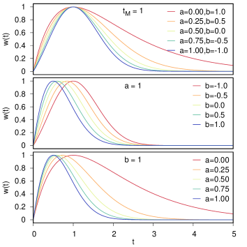
Figure 1: The shape of a Voigt-1D function. (top) The maximum value is fixed at $t_{\text{M}}=1$; (center) $a$ is fixed at 1; (bottom) $b$ is fixed at 1.

The Voigt-1D window has the following properties:

• The window function is the FID envelope $f(t)$ multiplied by $t$. The Fourier transform of $w(t)$ is $(i/2\pi)\hat{f}^{\prime}(x)$, where $\hat{f}(x)$ is the Fourier transform of the $f(t)$ , and $\hat{f}^{\prime}(x)$ is its first derivative. Using this relationship, we can show that the lineshape of the magnitude Fourier transform spectrum of the FID, after being multiplied with the window function, is exactly Voigt (see supplementary material, Section 1). This property ensures the ability of lineshape correction of the window function, except for extremely negative $b$ ($b<-2\sqrt{a}$), where sidelobes start to appear in the lineshape profile.

• The product of the window function $w(t;a,b)$ and an FID envelope $f(t;a_{0},b_{0})$ is still in the form of the window function $w(t;a^{\prime},b^{\prime})$, where parameters are updated as $a^{\prime}=a+a_{0}$, and $b^{\prime}=b+b_{0}$. That is,

  $$\begin{gathered}w(t;a,b)f(t;a_{0},b_{0})=\\ \frac{M(a+a_{0},b+b_{0})}{M(a,b)}w(t;a+a_{0},b+b_{0})\end{gathered}$$

• The ratio between $a$ and $b$ determines the shape of the window function. For a given $t_{\text{M}}$, $a$ increases as $b$ decreases, and larger $a$ generates a narrower window shape that approaches a Gaussian window. For a given $a$ or a given $b$, the increase of the other parameter result in a smaller $t_{\text{M}}$ and also narrower window. This property shows the wide tunability of the window function.

• The window function is independent of the FID length. In contrast to standard symmetric window functions, whose maximum is always at the center of the FID, the Voigt-1D window simply extends its values when the FID length is extended. This property ensures the result of windowing is not affected by experimental adjustments on the DAQ length, making it ideal for automatic processing of segmented chirped pulse data that cover multiple frequency bands.

2.2 Metrics for performance measurement

As widely accepted metrics in spectroscopy, SnR and FWHM characterize the intensity and the resolution of spectral lines, respectively. High SnR and narrow FWHM are often anti-correlated, which cannot be achieved simultaneously. We choose SnR/FWHM, in addition to SnR and FWHM, to measure the performance of the Voigt-1D window, so that maximizing SnR/FWHM reflects the goal of reaching highest possible SnR with highest possible spectral resolution.

Another implicit performance metric is the sampling density of the frequency grid, $\Delta\nu$, which is the reciprocal of the length of the time domain signal. In discrete Fourier transform, $\Delta\nu$ can be improved by zero-padding, i.e., appending certain length of $0$ arrays to the end of the original signal. The side-effect of zero-padding is to cause periodic ripples on the baseline due to spectral leakage.

2.3 Evaluation of the performance metrics: SnR

The SnR is evaluated by the ratio of the peak intensity and the noise level of the spectrum. These quantities can be calculated directly from mathematical formulae for any FID signal.

The peak intensity of an FID signal $f(t)$ from $t=0$ to $T$ is $\int_{0}^{T}f(t)\mathrm{d}t$. If the signal is multiplied by a window function $w(t)$, the peak intensity becomes $\int_{0}^{T}f(t)w(t)\mathrm{d}t$.

Assume the noise in the time domain is a pure white Gaussian noise with standard deviation of $\sigma$. The standard deviation of the magnitude Fourier transform of the noise, from $t=0$ to $T$, is $\sqrt{T}\sigma$. If the time domain white Gaussian noise is multiplied by a window function $w(t)$, the frequency domain noise has a standard deviation of $\sigma\sqrt{\int_{0}^{T}w^{2}(t)\mathrm{d}t}$ (see supplementary material, Section 2). For simplicity, we may assume $\sigma=1$. We may see that the noise of un-windowed FID grows to infinity as $T\rightarrow+\infty$, and therefore the upper bound $T$ needs to be specified for calculating the SnR. On the other hand, for a window function of which $\int_{0}^{+\infty}w^{2}(t)\mathrm{d}t$ is finite, the noise is also finite even when $T\rightarrow+\infty$.

Using the equations above, we can write the SnR of a windowed spectral line as

$$\text{SnR}(T)=\frac{\int_{0}^{T}f(t)w(t)\mathrm{d}t}{\sqrt{\int_{0}^{T}w^{2}(t)\mathrm{d}t}}$$ (5)

From Equation 5, the SnR of a un-windowed spectral line is

$$\text{SnR}(T)=\frac{\int_{0}^{T}f(t;a_{0},b_{0})\mathrm{d}t}{\sqrt{T}}=$$ (6)

$$\begin{cases}\cfrac{1-e^{-b_{0}T}}{b_{0}\sqrt{T}},\quad(a_{0}=0)\\ \cfrac{\sqrt{\pi}}{\sqrt{4a_{0}T}}e^{b_{0}^{2}/4a_{0}}\bigg{[}\text{erf}\Big{(}\cfrac{2a_{0}T+b_{0}}{\sqrt{4a_{0}}}\Big{)}-\text{erf}\Big{(}\cfrac{b_{0}}{\sqrt{4a_{0}}}\Big{)}\bigg{]},(a_{0}>0)\end{cases}$$

where $\text{erf}(x)=\cfrac{2}{\sqrt{\pi}}\int_{0}^{x}e^{-t^{2}}\mathrm{d}t$ is the error function. The maximum SnR is reached by finding the root of $\text{SnR}^{\prime}(T)=0$. In the $a_{0}=0$ case, the numerical result is $t_{\text{max}}\approx 1.26/b_{0}$, which was stated by Matson [4]. The maximum SnR at $t_{\text{max}}$ is approximately 0.715 (the $a_{0}=0$ case).

For the Voigt-1D window defined in Eq. 2, we consider the $T\rightarrow+\infty$ case because $\int_{0}^{+\infty}w^{2}(t)\mathrm{d}t$ is finite. We define the following two integrals:

$$P(a,b) =\int_{0}^{+\infty}t\exp(-at^{2}-bt)\mathrm{d}t$$ (7)

$$Q(a,b) =\int_{0}^{+\infty}t^{2}\exp(-2at^{2}-2bt)\mathrm{d}t$$ (8)

In the general case where $a>0$,

$$P(a,b) =\frac{1}{2a}-\frac{b\sqrt{\pi}}{4\sqrt{a^{3}}}\text{erfcx}\Big{(}\frac{b}{2\sqrt{a}}\Big{)}$$ (9)

$$Q(a,b) =\frac{\sqrt{2\pi}(a+b^{2})}{16\sqrt{a^{5}}}\text{erfcx}\Big{(}\frac{b}{\sqrt{2a}}\Big{)}-\frac{b}{8a^{2}}$$ (10)

where $\text{erfcx}(x)=e^{x^{2}}(1-\text{erf}(x))$ is the scaled complementary error function. In the Lorentzian-limited case where $a=0$,

$$P(0,b) =\int_{0}^{+\infty}te^{-bt}\mathrm{d}t=\frac{1}{b^{2}}$$ (11)

$$Q(0,b) =\int_{0}^{+\infty}t^{2}e^{-2bt}\mathrm{d}t=\frac{1}{4b^{3}}$$ (12)

With these two integrals, we can write the SnR of a Voigt-1D windowed spectral line, with FID decay parameters $(a_{0},b_{0})$ and window parameters $(a,b)$, as

$$s(a_{0},b_{0},a,b)=\frac{P(a_{0}+a,b_{0}+b)}{\sqrt{Q(a,b)}}$$ (13)

To find the maximum point of $s(a_{0},b_{0},a,b)$ with respect to $a$ and $b$, numerical method is necessary because its partial derivatives are transcendental functions that can only be solved numerically. In our computer code, we used standard least-square method to find the minimum of the negation of $s(a_{0},b_{0},a,b)$

2.4 Evaluation of the performance metrics: FWHM

The full widths of the spectral lines can only be calculated numerically. To find the full widths at level $y$, we simulated the spectral profile $f(x)$, find the numerical points that are closest to $f(x)=y$, and then measure the distance between these points. For un-windowed and Voigt-1D windowed spectra, we can write out the exact equations of $f(x)$, and therefore can simulate the spectral profile with a fine $x$ grid numerically. For Kaiser windowed spectra, we do not have the exact lineshape function, and therefore the spectral profile is generated by digital Fourier transform, and smoothed by univariate spline interpolation.

2.5 Determination of FID initial parameters $a_{0}$ and $b_{0}$

The value of the performance metrics are not only the function of the window function, but also the shape of the original FID that is controlled by the initial parameters $a_{0}$ and $b_{0}$. In the derivations above, we set the start of DAQ as $t=0$. This frame of reference simplifies the mathematical expressions of the window function and performance metrics. In real chirped pulse experiments, however, the chirp excitation has a noticeable duration $t_{\text{cp}}$. In addition, a certain dead time $t_{\text{d}}$ is often placed between the end of excitation and the start of DAQ, so that electronics can be correctly switch on or off, and transient noises can be blocked. Figure 2 illustrates the relations between these times. In this frame of reference, the actual start of the FID of a molecular line is $-t_{0}$ ($t_{0}>0$) in Figure 2, which is between $-t_{\text{d}}$ and $-t_{\text{d}}-t_{\text{cp}}$ and can be calculated if the excitation frequency is known (see Supplementary Material, Section 3.6).

Figure 2: Illustration of the reference frame of time in a chirped pulse experiment.

The presence of $t_{0}$ affects the shape of the FID envelope. Let $b_{\lambda}$ to be the real Lorentzian component of the FID, we may write the FID envelope as

$$f(t) =\exp(-a_{0}(t+t_{0})^{2}-b_{\lambda}(t+t_{0}))$$ (14)

$$=\exp(-a_{0}t^{2}-(b_{\lambda}+2a_{0}t_{0})t)\cdot\exp(-a_{0}t_{0}^{2}-b_{\lambda}t_{0})$$

Compared with Equation 1, we have $b_{0}=b_{\lambda}+2a_{0}t_{0}$, i.e., the exponential decay term depends not only on the real broadening effect due to physics, but also on the Gaussian decay term and delay time $t_{0}$ due to mathematical relations. The extra intensity scalar $\exp(-a_{0}t_{0}^{2}-b_{\lambda}t_{0})$ represents the loss of line intensity due to $t_{0}$, which is discussed by Gerecht et al.[14]. The effect of $t_{0}$ is independent of the choice of frame of reference.

When the FID is Lorentzian dominated, i.e., $b_{\lambda}\geq a_{0}$, the effect of $t_{0}$ is not obvious. However, when the FID is Doppler dominated, the effect can be significant. Doppler dominated FID occurs both in room-temperature (sub)millimeter chirped pulse spectroscopy, where the Doppler broadening of the molecular line is not negligible, and in jet cooled spectroscopy, both microwave and (sub)millimeter, where the residual Doppler components from the jet is the main dephasing mechanism.

The optimization of Voigt-1D window function parameters depends on the FID initial parameters $a_{0}$ and $b_{0}$, and therefore implicitly depends on $t_{0}$. For a narrowband chirp, or single line excitation, $t_{0}$ can be precisely calculated and therefore this effect can be precisely accounted for in Equation 13. For a broadband chirp, each line has its unique $t_{0}$ that spans the whole chirp excitation, and this effect is especially significant when $a_{0}t_{0}\geq b_{\lambda}$. A window function, however, has an explicit shape that cannot be the optimal choice for all the $t_{0}$ possibilities. It is inevitable that compromise has to be made, and in this paper, we choose to use the center point of the chirp excitation, $t_{\text{d}}+t_{\text{cp}}/2$, as the “averaged” $t_{0}$ to determine the window function parameters.

2.6 Unit convention

In deriving the mathematical expressions, we did not specify the units of $t$, $a$, and $b$. $a$ has the dimension of time^-2, and $b$ has the dimension of time^-1. Our mathematical derivations can be rescaled to any unit system without altering their properties, as long as $at^{2}$ and $bt$ are kept dimensionless, and the ratio $b/2\sqrt{a}$ remains unchanged. In our data treatment, we use $\upmu$s for $t$, and therefore $a$ is in MHz² and $b$ is in MHz.

3 Results and Discussion

3.1 Choice of window parameters based on theoretical SnR

Figure 3 visualizes Eq. 13 and its corresponding FWHM as a function of $a$ and $b$ for given $(a_{0},b_{0})$ pairs. We calculated three sets: $(a_{0},b_{0})=(1,0)$ for pure Gaussian decay, $(a_{0},b_{0})=(0,1)$ for pure exponential decay, and an intermediate case $(a_{0},b_{0})=(0.25,1)$, so that $b=2\sqrt{a}$. Interestingly, the maxima of both SnR and SnR/FWHM are reached when $a=0$, i.e., the Voigt-1D function is in fact a pure first derivative of the Lorentzian. It can be justified by two reasons. First, when $a=0$, the area under the window function is the largest (see Figure 1), and therefore the window function collects the most signal. Second, the FWHM is smaller when $a=0$ because the window function maximizes the Lorentzian component in the line profile. The $b$ value for maximum SnR/FWHM is approximately half of the $b$ value for maximum SnR.

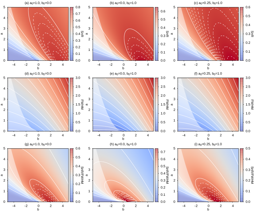
Figure 3: Theoretical SnR (top row), FWHM $\gamma_{V}$ (center row), and SnR/FWHM (bottom row) at the $T\rightarrow+\infty$ limit. (a,d,g) $a_{0}=1.0,b_{0}=0$, (b,e,h) $a_{0}=0,b_{0}=1.0$, (c,f,i) $a_{0}=0.25,b_{0}=1.0,b=2\sqrt{a}$. In the SnR and SnR/FWHM plots, the solid contour lines are spaced by 0.1, and the dashed contour lines are spaced by 0.01 For the FWHM plots, the solid contour lines are spaced by 0.2. The shaded areas in all plots mark the unfavored negative $b$ values where $b<-2\sqrt{a}$.

Under the guide of Eq. 13 and the numerical methods used to generate Figure 3, one can find an optimal $(a,b)$ parameter set of the Voigt-1D window for a particular FID signal, according to the metric to be optimized. To find this parameter set, the initial parameters $(a_{0},b_{0})$, in other words, the Gaussian ($\gamma_{G}$) and Lorentzian ($\gamma_{L}$) FWHM of the original FID signal, need to be determined. If fitting the envelope of the FID is convenient, one can retrieve $(a_{0},b_{0})$ from the time domain fit. If not, fitting a complex Voigt profile to the un-windowed frequency domain spectrum may also lead to a reasonable estimation of $a$ and $b$. Especially, a priori one may fix $a$ to $\pi^{2}\gamma_{G}^{2}/(4\ln 2)$, assuming that $a$ is completely caused by Doppler broadening of the molecule. Although no analytical expression of obtaining the optimal $(a,b)$ parameters can be specified, this procedure to find optimal parameter sets can be easily programmed or tabulated to allow automatic processes.

Figure 3 also demonstrates the wide tunability of the Voigt-1D window function. Around the maxima, there is a wide range of $a$ and $b$ that can yield SnR and SnR/FWHM values more than 90 % of the theoretical maxima. At a given SnR, a series of $(a,b)$ pairs can be chosen to produce different FWHM. In turn, $(a,b)$ pairs on the same contour line in the center row of Figure 3 produce identical FWHM with different weights of the Gaussian and Lorentzian components. Such tunability is helpful when we apply the window function to broadband spectra, where the Doppler component intrinsically varies across the whole spectra. We can show that using the “averaged” window parameters derived from the “averaged” $t_{0}$ can produce SnR and SnR/FWHM near the optimal values across the broadband chirps (See Supplementary Material, Section 4.1).

The flexibility of the Voigt-1D window allows the user to tune the window away from its “optimal” performance. For example, if high resolution is the priority, both $a$ and $b$ need to be as small as possible, because the line width metrics always monotonously increases as $b$ increases for any given $a$, and as $a$ increases for any given $b$. $a=a_{0}$ and $b=-2\sqrt{a_{0}}$ can be a good initial parameter set, and one may further adjust $a$ and $b$ following the constraint $b=-2\sqrt{a}$ for maintaining good lineshape, until a satisfactory resolution is achieved. In this scenario, negative $b$ does not infer anything about an exponentially increasing FID, which is impossible, but servers only as a mathematical treatment to obtain narrow linewidths, at the cost of losing SnR.

3.2 SnR enhancement on single-peak spectra

The performance of the Voigt-1D window was first tested on a set of OCS lines, consisting of 51 entries. These lines were experimentally measured using a millimeter wave chirped pulse spectrometer[22] (See Supplementary Material, Section 3.1 for experimental details). In this data set, each line is the only line within its chirp bandwidth, so that the $(a_{0},b_{0})$ parameters of the FID envelope can be unambiguously modeled. We chose the lines from the OC^34S isotopologue and the $v_{2}=1$ vibrational excited state of the parent isotopic species, in order to avoid saturation effects on the ground state lines of the latter. The line frequencies range from the 60 GHz to 300 GHz, where the lineshape shifts from Lorentzian-dominated to nearly equal weight of Lorentzian and Gaussian components.

For each entry, we treated the data with 2 sets of Voigt-1D window parameters, set (1) optimized for maximizing SnR, and set (2) optimized for maximizing SnR/FWHM. Before applying the Voigt-1D window, we retrieved the initial $a_{0}$ and $b_{0}$ values of the line by fitting the time domain FID signal (see supplementary material, Section 3.4). In the fit, $a_{0}$ is fixed to $\pi^{2}\gamma_{G}^{2}/(4\ln 2)$, where $\gamma_{G}$ is the Doppler FWHM of the OCS line, and $b_{0}$ is fitted from the FID. Afterwards, the two parameter sets were numerically solved by fixing $a=0$, as demonstrated in Figure 3. The results were compared with 3 sets of Kaiser window $\pi\alpha$ values, 0, 4, and 8. $\pi\alpha=0$ is equivalent to un-windowed spectrum, $\pi\alpha=8$ is heavily windowed for best baseline resolution, and then $\pi\alpha=4$ is the medium state between un-windowed and heavily windowed spectra. Before applying the Kaiser windows, the FID signal was truncated to the length that maximizes theoretical SnR of the un-windowed spectrum (Equation 6).

Figure 4 shows the SnR (top panel), FWHM (center panel), and SnR/FWHM (bottom panel) of all 51 entries. In all three plots, the results of the un-windowed spectra, i.e., Kaiser $\pi\alpha=0$, are shown as gray bars in the background, providing the reference point for comparison. The enhancement of the four windows are plotted as line series. 100 % means that the value to be compared (SnR, FWHM, or SnR/FWHM) of the windowed line is identical to the un-windowed line. Note that the 51 entries are independent samples, and therefore the line series are only for visual distinction and does not indicate any correlation between entries.

The performance of four tested windows are summarized as the following:

(1) The SnR. For almost all entries, the Voigt-1D window produces spectral lines of higher SnR than the un-windowed lines, which are already of the highest SnR in theory. This is because the noise in the real FID signals is not pure white noise, and may vary from shot to shot. The Voigt-1D window, however, is insensitive to truncation and therefore can be applied to a long FID record and collect as much information as possible. Two parameter sets of the Voigt-1D window result in similar SnR enhancements, which corresponds to the large tunable parameter space shown in Figure 3. Kaiser windows also improve the SnR in most cases, but the enhancement is less than that from Voigt-1D windows. The higher SnR enhancement by Voigt-1D window can be explained because the Voigt-1D window does not truncate data. The window shape weights the data points such that the noise is suppressed, but it still uses all the information of the full data series. The Kaiser window, on the other hand, has to discard the data after a certain length in exchange for higher SnR, because the Kaiser window has a rigid symmetric window shape.

(2) The FWHM. For all entries, the un-windowed spectra present the smallest FWHM. It is not surprising because applying window function in the time domain is equivalent to convolving the window function profile with the spectral line profile. Nevertheless, the Voigt-1D set (2) only broadens the line by approximately 25 %. These values demonstrate that the Voigt-1D set (2) window does not severely broaden the line in exchange for SnR enhancement. The FWHM produced by Voigt-1D set (1) is similar to that produced by Kaiser window with $\pi\alpha=4$. The FWHM is almost doubled. Finally, Kaiser window with $\pi\alpha=8$ produces 2.5 times broader FWHM.

(3) The SnR/FWHM. Following the discussion of SnR and FWHM, it is expected that Voigt-1D set (2) produces the optimal SnR/FWHM among the 4 tested windows. This window proves that a slight line broadening in exchange for a significant SnR improvement is feasible. Voigt-1D set (1) is in second place, and has higher SnR/FWHM than Kaiser $\pi\alpha=4$, because they produce similar FWHMs but Voigt-1D set (1) produces higher SnR. The Kaiser $\pi\alpha=8$ window has disadvantage in this SnR/FWHM metric, because this window significantly broadens the spectral lines. Nevertheless, Kaiser $\pi\alpha=8$ will have better result if the focus is on baseline resolution, which is important in some applications, such as the identification of isotopologue species in their natural abundances[9].

In addition, applying the Voigt-1D window can help improving frequency sampling together with the SnR enhancement, because of its insensitivity to zero-padding. In the tests discussed above, the high SnR spectra were obtained by FID truncation, and no zero-padding was applied. There are only 3–5 points to describe a line in the frequency domain spectrum. To improve frequency sampling, extending the FID or zero-padding is necessary. Shown in Equations 7–13, Voigt-1D window does not lose SnR in zero-padding. Also, since the window function starts at 0, it suppresses the baseline ripples due to spectral leakage. These ripples, although are not real noise in nature, contaminates the spectral baseline and produces effective larger noise in our SnR calculation. Examples of such ripples can be found in Figure S2. Therefore, if zero-padding is used, the SnR of the un-windowed spectra shown in Figure 4 will be lower, and the SnR enhancement by Voigt-1D window calculated in this way will be higher than what has been presented. The Kaiser window also suppresses these ripples, but only with sufficient large $\pi\alpha$ values (e.g., $>5.6$), which broadens the FWHM.

Figure 4: Summary of SnR (top), FWHM (center), and SnR/FWHM (bottom) of 51 OCS lines, treated with Voigt-1D windows and Kaiser windows. For Voigt-1D windows, parameter set (1) was set to maximizing SnR, and set (2) was set to maximize SnR/FWHM. For Kaiser windows ($\pi\alpha=0,4,8$), the FID signal is truncated to the time that maximizes Equation 13, the theoretical SnR of the un-windowed spectra. In all panels, the metrics from the un-windowed spectra, i.e., Kaiser $\pi\alpha=0$, is plotted as gray bars towards the left axis. The metrics of the rest 4 windows are plotted line point series towards the right axis, on the scale of the enhancement percentage. The dashed line marks the 0 % enhancement level, i.e., the value of the metric is equal to the case of the un-windowed spectra.

3.3 Preservation of frequency resolution on partially resolved spectra

In some scenarios, the frequency resolution is more important than the SnR. With the wide tunability of the Voigt-1D window, it is able to produce spectra with small FWHMs. To evaluate to which degree can the Voigt-1D window preserve the frequency resolution, we measured the $J_{10\leftarrow 9},K=9$ line of CH3CN at 183676 MHz, exhibiting a partially resolved hyperfine structure. The hyperfine splitting is $\sim 0.8$ MHz, and the Doppler-broadening limit of CH3CN is $0.36$ MHz at room temperature. Therefore, the hyperfine splitting is marginally resolvable under the Doppler-broadening limit.

Figure 5 shows the FID signal of a 60 MHz chirp around the $K=9$ line of pure CH3CN vapor measured at 4 $\upmu$bar. The DAQ delay $t_{\text{d}}$ was set to 256 ns. According to the CDMS catalog[23], the hyperfine splitting of this line has 3 strong components at 183675.955 ($F_{10\leftarrow 9}$), 183676.690 ($F_{11\leftarrow 10}$), and 183676.787 MHz ($F_{9\leftarrow 8}$), with relative intensity of 0.997, 1.103, and 0.901. Since the $F_{11\leftarrow 10}$ and $F_{9\leftarrow 8}$ components are spaced less than 0.1 MHz, they are unresolvable due to Doppler-broadening. Therefore, we may simplify the splitting structure into two frequency components which differ by 0.7835 MHz and roughly have a intensity ratio of 1:2. In Figure 5, the beating of the two frequency components is visible at a period of 1/0.7835 MHz $\approx 1.28$ $\upmu$s. We can directly fit this FID as a product of the decay envelope and the beating of two sine waves (see supplementary material, Section 3.4). We fix $a_{0}=0.4508$ MHz², and retrieved $b_{0}=1.005(16)$ MHz.

Figure 5: The FID of the $J_{10\leftarrow 9},K=9$ line of CH3CN at 183676 MHz, fitted to $f(t)=\exp(-0.4508t^{2}-1.005(16)t)$. The DAQ delay is 256 ns. The LO frequency of this FID is at 183720 MHz, and the chirp bandwidth is 60 MHz. The blue trace shows the FID signal, the red trace shows the least-squared fit, and the black trace shows the fit residual (shifted for clarity).

Although the beating envelope is apparent in the time domain, the un-windowed spectrum in the frequency domain completely squeezes the two frequency components into a single peak (Figure 6, top panel). To resolve the two components, frequency resolution, instead of SnR, is the primary goal. To begin, we first adjusted the truncation length (3.3 $\upmu$s) of the Kaiser window ($\pi\alpha=8$) so that the two peaks are just about to separate. Then, we calculated the Voigt-1D window parameters for high resolution, $a=a_{0}=0.4508$ and $b=-2\sqrt{a_{0}}=-1.3428$. The fit results of the windowed spectra are also presented in Figure 6. Both windows are able to resolve the two hyperfine components. In the presented results, the Kaiser window forms slightly wider FWHM and also higher SnR than the Voigt-1D window. Since the resolution power can be continuously tuned by adjusting the window parameters, the Voigt-1D window may be considered having similar performance as the Kaiser window.

Figure 6: Fit results of the $J_{10\leftarrow 9},K=9$ spectral line of CH3CN, treated by the Voigt-1D window and Kaiser window. The spectral intensities are normalized to unity to ease the visual comparison of the noise level. The black curve shows the spectrum, the red curve shows the overall fit, and the colored areas (blue and yellow) show the individual components of the fit. The fit residual is plotted below each spectrum. The red vertical sticks shows the catalog frequency and intensity of the 3 strong hyperfine components. The noise level is estimated using the standard deviation of the fitted residuals.

It is worth mentioning that, the low frequency beating envelope produced by two closely separated frequency components does create a pitfall for parameter selection algorithm of the Voigt-1D windows optimized for highest SnR or SnR/FWHM. The parameter selection based on the results in Section 2.3, demonstrated in Figure 3, leads to zero Gaussian component in the Window function. In this scenario, the window function has a sharp rise at the beginning of the FID, which may coincidentally interfere with the strong beating FID envelope, As a result, the spectral lineshape can be altered significantly, presenting asymmetric features. The readers are referred to Section 4.3 in the supplementary material for a detailed discussion. Nonetheless, by constraining the $b$ parameter of the Voigt-1D window to $-b_{0}$, so that the majority of the exponential decay in the original FID signal is cancelled out by the window function, we can obtain spectral lines with close-to-optimal SnR and correct lineshape.

3.4 Overall performance on broadband spectrum

The performance of the Voigt-1D window on room-temperature broadband chirped pulse spectra are tested by numerical simulation, because the bandwidth of our DDS-based chirped pulse spectrometer is limited to 0.5 GHz. Two simulations were performed, one at 2–10 GHz to simulate Lorentzian-dominated microwave chirped pulse spectra, and one at 640–650 GHz to simulate Doppler-dominated submillimeter chirped pulse spectra. The lines of cis-furfural (C4H3OCHO) [24] were used to simulate the microwave chirp, and the lines of N-methylformamide (HCONHCH3) [25] were used to simulate the submillimeter chirp. A Lorentzian FWHM of 0.1 MHz was used universally for both simulations. More details of the simulation can be found in supplementary material, Section 3.6. In this simulation, we compared the results of the two Voigt-1D window parameter sets, and the result of the Kaiser window ($\pi\alpha=8$).

Figure 7 shows the simulation of the C4H3OCHO spectrum, and Figure 8 shows the simulation of the HCONHCH3 spectrum. In both simulations, the SnR enhancement of the Voigt-1D window behaves as expected. The figures show that the noise level of the un-windowed spectra is similar to the Kaiser windowed spectra, and is slightly higher than the spectra from Voigt-1D set (2) window. Voigt-1D set (1) window produces spectra with noticeable lower noise which can be observed by eye. The dashed square box in Figure 7 also highlights a weaker line next to a stronger line that is visually more distinct in the Voigt-1D set (1) windowed spectrum than other spectrum. The lineshape of the un-windowed magnitude spectra is corrected by the Voigt-1D window, as well as the Kaiser window. Overall, the peak resolution of the Voigt-1D set (2) window is similar to the Kaiser window because of their similar FWHM. In the right bottom panel of Figure 7, a case shows that Voigt-1D set (2) window performs better in resolving a closely spaced doublet than the Kaiser window, because it produces less Gaussian component in the Voigt profile. On the other hand, Kaiser window produces best baseline resolution, which is especially useful in identifying lines in the congested regions marked out by dashed square boxes in Figure 8.

Figure 7: Simulated broadband chirped pulse spectrum of C4H3OCHO between 2–10 GHz. The top left panel shows the FID, the top right panel shows the overall spectrum, and the bottom panels show zoomed-in regions. Red sticks in the bottom panels show the expected transitions from the line catalog. The maximum line intensity is normalized to unity for all traces so that the SnR can be directly compared by measuring the noise only. Voigt-1D set (1) uses $(a,b)=(0,0.9461\text{ MHz})$ for maximizing SnR, and Voigt-1D set (2) uses $(a,b)=(0,\text{ 0.3170})$ for maximizing SnR/FWHM.

Figure 8: Simulated broadband chirped pulse spectrum of HCONHCH3 at 640–650 GHz. The top left panel shows the FID, the top right panel shows the overall spectrum, and the bottom panels show zoomed-in regions. Red sticks in the bottom panels show the expected transitions from the line catalog. The maximum line intensity is normalized to 1 for all traces so that the SnR can be directly compared by measuring the noise only. Voigt-1D set (1) uses $(a,b)=(0,15.7789\text{ MHz})$ for maximizing SnR, and Voigt-1D set (2) uses $(a,b)=(0,6.5515\text{ MHz})$ for maximizing SnR/FWHM.

4 Conclusion

In conclusion, we have proposed a specific window function, noted as the “Voigt-1D” window, for treating the data of chirped pulse experiments. The window function takes the form $w(t;a,b)=t\exp(-at^{2}-bt)/M$, where $t$ is the time variable, $a$ and $b$ are two adjustable parameters, and $M$ is the normalization factor. The window function corrects the spectral lineshape, offers wide tunability by adjusting its two parameters, suppresses baseline ripples from zero-padding, and is able to generate high SnR spectra with properly chosen parameters. We have derived the mathematical SnR equations for a chirped pulse spectral line treated by the Voigt-1D window, and discussed the guideline of parameter selection based on these mathematical expressions. The programmable routines to find two optimal parameter sets, one for achieving maximum SnR, and one for achieving maximum SnR/FWHM, are proposed.

Performance of the Voigt-1D window is evaluated by treating real chirped pulse experimental data of OCS and CH3CN lines, and by treating simulated broadband chirped pulse data. The results are compared with un-windowed magnitude Fourier transform spectra, and with results treated by Kaiser-Bessel windows, which are commonly used in current chirped pulse literature. Our results show that the Voigt-1D window with maximum SnR/FWHM is able to enhance the SnR by 100 % on average, and sometimes up to 250 % than the un-windowed magnitude spectra, at a cost of only 25 % wider FWHM. The Voigt-1D window with maximum SnR can achieve slightly higher SnR enhancement at the cost of almost doubling the FWHM of the un-windowed spectra. Compared with Kaiser window ($\pi\alpha=4$), the SnR enhancement of the Voigt-1D window is higher, whereas the FWHM broadening is lower. When resolving closely spaced lines with similar intensities, the Voigt-1D is able to reach similar, and sometimes better, performance to the Kaiser window ($\pi\alpha=8$). When baseline resolution is the primary goal, such as decomposing congested spectra and identifying weak satellite lines on the wings of strong lines, Kaiser window is still the preferred choice.

5 Supplementary material

Supplementary material includes additional mathematics of the Voigt-1D window, experimental, simulation, and data fitting details, as well as some supplementary results such as the performance of “averaged” window parameters on broadband chirp. The supporting Python code for the optimization of Voigt-1D window function parameters is available at https://doi.org/10.5281/zenodo.4555759 and from the authors upon reasonable request.

6 Acknowledgement

The authors thank the anonymous referees for helpful comments that improved the quality and robustness of this manuscript. This work was funded by the French ANR Labex CaPPA through the PIA under Contract No. ANR-11-LABX-0005-01, the Regional Council of Hauts-de-France, the European Funds for Regional Economic Development (FEDER), and the contract CPER CLIMIBIO. L. Zou thanks the financial support from the European Union’s Horizon 2020 research and innovation programme under the Marie Skłodowska-Curie Individual Fellowship grant No. 894508.

7 Contributor Statement

Luyao Zou: Methodology, Investigation, Formal analysis, Visualization, Writing - Original Draft, Writing - Review & Editing. Roman Motiyenko: Conceptualization, Methodology, Writing - Review & Editing, Supervision.

References

- [1] R. R. Ernst, W. A. Anderson, Application of Fourier Transform Spectroscopy to Magnetic Resonance, Rev. Sci. Instrum. 37 (1) (1966) 93–102. doi:10.1063/1.1719961.
- [2] T. J. Balle, W. H. Flygare, Fabry-Perot cavity pulsed Fourier transform microwave spectrometer with a pulsed nozzle particle source, Rev. Sci. Instrum. 52 (1) (1981) 33–45. doi:10.1063/1.1136443.
- [3] G. G. Brown, B. C. Dian, K. O. Douglass, S. M. Geyer, S. T. Shipman, B. H. Pate, A broadband Fourier transform microwave spectrometer based on chirped pulse excitation, Rev. Sci. Instrum. 79 (5). doi:10.1063/1.2919120.
- [4] G. B. Matson, Signal integration and the signal-to-noise ratio in pulsed NMR relaxation measurements, Journal Magnetic Resonance (1969) 25 (3) (1977) 477 – 480. doi:10.1016/0022-2364(77)90210-4.
- [5] D. D. Traficante, M. Rajabzadeh, Optimum window function for sensitivity enhancement of NMR signals, Concepts in Magnetic Resonance 12 (2) (2000) 83–101.
- [6] M. R. Palmer, C. L. Suiter, G. E. Henry, J. Rovnyak, J. C. Hoch, T. Polenova, D. Rovnyak, Sensitivity of Nonuniform Sampling NMR, J. Phys. Chem. B 119 (22) (2015) 6502–6515. doi:10.1021/jp5126415.
- [7] B. Simon, H. Köstler, Improving the sensitivity of FT-NMR spectroscopy by apodization weighted sampling, J. Biomol. NMR 73 (3-4) (2019) 155–165. doi:10.1007/s10858-019-00243-7.
- [8] M. Kaur, C. M. Lewis, A. Chronister, G. S. Phun, L. J. Mueller, Non-Uniform Sampling in NMR Spectroscopy and the Preservation of Spectral Knowledge in the Time and Frequency Domains, J. Phys. Chem. A 124 (26) (2020) 5474–5486, pMID: 32496067. doi:10.1021/acs.jpca.0c02930.
- [9] C. Pérez, S. Lobsiger, N. A. Seifert, D. P. Zaleski, B. Temelso, G. C. Shields, Z. Kisiel, B. H. Pate, Broadband Fourier transform rotational spectroscopy for structure determination: The water heptamer, Chem. Phys. Lett. 571 (2013) 1 – 15. doi:https://doi.org/10.1016/j.cplett.2013.04.014.
- [10] I. Uriarte, F. Reviriego, C. Calabrese, J. Elguero, Z. Kisiel, I. Alkorta, E. J. Cocinero, Bond length alternation observed experimentally: The case of 1H-indazole, Chem. Eur. J. 25 (43) (2019) 10172–10178.
- [11] B. C. Dian, G. G. Brown, K. O. Douglass, B. H. Pate, Measuring picosecond isomerization kinetics via broadband microwave spectroscopy, Science 320 (5878) (2008) 924–928.
- [12] K. Prozument, G. B. Park, R. G. Shaver, A. K. Vasiliou, J. M. Oldham, D. E. David, J. S. Muenter, J. F. Stanton, A. G. Suits, G. B. Ellison, et al., Chirped-pulse millimeter-wave spectroscopy for dynamics and kinetics studies of pyrolysis reactions, Phys. Chem. Chem. Phys. 16 (30) (2014) 15739–15751.
- [13] B. M. Hays, T. Guillaume, T. S. Hearne, I. R. Cooke, D. Gupta, O. A. Khedaoui, S. D. Le Picard, I. R. Sims, Design and performance of an E-band chirped pulse spectrometer for kinetics applications: OCS–He pressure broadening, J. Quant. Spectrosc. Radiat. Transfer 250 (2020) 107001.
- [14] E. Gerecht, K. O. Douglass, D. F. Plusquellic, Chirped-pulse terahertz spectroscopy for broadband trace gas sensing, Opt. Express 19 (9) (2011) 8973–8984. doi:10.1364/OE.19.008973.
- [15] K. N. Crabtree, M.-A. Martin-Drumel, G. G. Brown, S. A. Gaster, T. M. Hall, M. C. McCarthy, Microwave spectral taxonomy: A semi-automated combination of chirped-pulse and cavity Fourier-transform microwave spectroscopy, J. Chem. Phys. 144 (12) (2016) 124201.
- [16] G. B. Park, R. W. Field, Perspective: The first ten years of broadband chirped pulse Fourier transform microwave spectroscopy, J. Chem. Phys. 144 (20) (2016) 200901.
- [17] A. L. Steber, B. J. Harris, J. L. Neill, B. H. Pate, An arbitrary waveform generator based chirped pulse Fourier transform spectrometer operating from 260 to 295GHz, J. Mol. Spectrosc. 280 (2012) 3 – 10. doi:https://doi.org/10.1016/j.jms.2012.07.015.
- [18] J. L. Neill, B. J. Harris, A. L. Steber, K. O. Douglass, D. F. Plusquellic, B. H. Pate, Segmented chirped-pulse Fourier transform submillimeter spectroscopy for broadband gas analysis, Opt. Express 21 (17) (2013) 19743–19749. doi:10.1364/OE.21.019743.
- [19] C. Abeysekera, L. N. Zack, G. B. Park, B. Joalland, J. M. Oldham, K. Prozument, N. M. Ariyasingha, I. R. Sims, R. W. Field, A. G. Suits, A chirped-pulse Fourier-transform microwave/pulsed uniform flow spectrometer. II. Performance and applications for reaction dynamics, J. Chem. Phys. 141 (21) (2014) 214203. doi:10.1063/1.4903253.
- [20] M. Fatima, C. Pérez, B. E. Arenas, M. Schnell, A. L. Steber, Benchmarking a new segmented K-band chirped-pulse microwave spectrometer and its application to the conformationally rich amino alcohol isoleucinol, Phys. Chem. Chem. Phys. 22 (2020) 17042–17051. doi:10.1039/D0CP01141J.
- [21] G. Turin, An introduction to matched filters, IRE Transactions on Information Theory 6 (3) (1960) 311–329. doi:10.1109/TIT.1960.1057571.
- [22] L. Zou, R. A. Motiyenko, L. Margulès, E. A. Alekseev, Millimeter-wave emission spectrometer based on direct digital synthesis, Rev. Sci. Instrum. 91 (6) (2020) 063104. doi:10.1063/5.0004461.
- [23] H. Müller, F. Schlöder, J. Stutzki, G. Winnewisser, The Cologne Database for Molecular Spectroscopy, CDMS: a useful tool for astronomers and spectroscopists, J. Mol. Struct. 742 (1-3) (2005) 215 – 227. doi:10.1016/j.molstruc.2005.01.027.
- [24] R. Motiyenko, E. Alekseev, S. Dyubko, F. Lovas, Microwave spectrum and structure of furfural, J. Mol. Spectrosc. 240 (1) (2006) 93 – 101. doi:10.1016/j.jms.2006.09.003.
- [25] Belloche, A., Meshcheryakov, A. A., Garrod, R. T., Ilyushin, V. V., Alekseev, E. A., Motiyenko, R. A., Margulès, L., Müller, H. S. P., Menten, K. M., Rotational spectroscopy, tentative interstellar detection, and chemical modeling of N-methylformamide, A&A 601 (2017) A49. doi:10.1051/0004-6361/201629724.