Splitting the Sample at the Largest Uncensored Observation

Abstract

We calculate finite sample and asymptotic distributions for the largest censored and uncensored survival times, and some related statistics, from a sample of survival data generated according to an iid censoring model. These statistics are important for assessing whether there is sufficient follow-up in the sample to be confident of the presence of immune or cured individuals in the population. A key structural result obtained is that, conditional on the value of the largest uncensored survival time, and knowing the number of censored observations exceeding this time, the sample partitions into two independent subsamples, each subsample having the distribution of an iid sample of censored survival times, of reduced size, from truncated random variables. This result provides valuable insight into the construction of censored survival data, and facilitates the calculation of explicit finite sample formulae. We illustrate for distributions of statistics useful for testing for sufficient follow-up in a sample, and apply extreme value methods to derive asymptotic distributions for some of those.

2103.01337

and

1 Introduction

In the analysis of censored survival data, it was long considered an anomalous situation to observe a sample Kaplan-Meier estimator (KME) [7] which is improper, i.e., of total mass less than 1. This occurs when the largest survival time in the sample is censored. In some early treatments it was advocated to remedy this situation by redefining the largest survival time in the sample to be uncensored (cf. Gill [3], p.35). Later it was recognized that one or more of the largest observations being censored conveys important information concerning the possible existence of immune or cured individuals in the population. One aim of the present paper is to focus attention on the importance of considering the location and conformation of the censored observations in the sample.

Even in a population in which no immunes are present, it can be the case that the largest or a number of the largest survival times are censored according to whatever chance censoring mechanism is operating in the population. The possible presence of immunes will be signaled by an interval of constancy of the KME at its right hand end, with the largest observation being censored. The length of that interval and the number of censored survival times larger than the largest uncensored survival time are important statistics for testing for the presence of immunes, and for assessing whether there is sufficient follow-up in the sample to be confident of their presence. We focus particularly on the “sufficient follow-up” issue in the present paper.

Our aim is to derive distributional results that lead to rigorous methods for deciding if the population contains immunes and if the length of observation is sufficient. We proceed by calculating finite sample and asymptotic joint distributions for the largest censored and uncensored survival times under an iid (independent identically distributed) censoring model for the data. These calculations are facilitated by a significant splitting result which states that, conditional on knowing both the value of the largest uncensored survival time and the number of censored observations exceeding this observation, the sample partitions into two conditionally independent subsamples. The observations in each subsample have the distribution of an iid sample of censored survival times, of reduced size, from appropriate truncated random variables. See Theorem 2.1 below for a detailed description of this result.

Using this result we are able to calculate expressions for distributions of statistics, such as those mentioned, related to testing for sufficient follow-up. Those distributions are reported in Section 2. In Section 3 we calculate large sample distributions for the statistics under very general conditions on the tails of the censoring and survival distributions. Special emphasis is placed on the realistic situation where the censoring distribution has a finite right endpoint. These results complement analysis in [10] made under the assumption of an infinite right endpoint. That paper is concerned only with asymptotics whereas in the present paper we have the finite sample distributions in Section 2. With these we can calculate moments of rvs, etc.

A discussion Section 4 contains a motivating example outlining how the results can be applied in practice to validate and improve existing procedures. Proofs for the formulae in Section 2 are in Section 5 and the asymptotic results are proved in Section 6. A supplementary arXiv submission [11] contains plots illustrating some of the distributions in Section 2.

For further background we refer to the book by Maller and Zhou [9] which gives many practical examples from medicine, criminology and various other fields of this kind of data and its analysis. See also the review articles by Othus, Barlogie, LeBlanc and Crowley [12], Peng and Taylor [14], Taweab and Ibrahim [17], Amico and Van Keilegom [1], and a recent paper by Escobar-Bach, Maller, Van Keilegom and Zhao [2].

2 Splitting the Sample: Finite Sample Results

2.1 Setting up: the iid censoring model

We assume a general independent censoring model with right censoring and adopt the following formalism. Assume $F(x)$ and $G(x)$ are two proper, continuous, cumulative distribution functions (cdfs) on $[0,\infty)$. Let $p\in(0,1]$ be a parameter. Define the iid sequence of triples $\{(L_{i},U_{i},B_{i}),i\geq 1\}$, where $L_{i}$ has distribution $F$, $U_{i}$ has distribution $G$ and $B_{i}$ is Bernoulli with

$$P(B_{i}=1)=1-P(B_{i}=0)=p.$$

For each $i$ the components $L_{i}$, $U_{i},$ and $B_{i}$ are assumed mutually independent. The $U_{i}$ are censoring variables and the $L_{i}$ represent lifetimes given that they are finite. Define

$$T_{i}^{*}=\infty\cdot(1-B_{i})+L_{i}B_{i}=\begin{cases}\infty,&\text{ if }B_{i}=0,\\ L_{i},&\text{ if }B_{i}=1.\end{cases}$$

Then $T_{i}^{*}$ has distribution $F^{*}$ given as

$$P(T_{i}^{*}\leq x)=F^{*}(x):=pF(x),\,0\leq x<\infty,\ \text{and}\ P(T_{i}^{*}=\infty)=1-p.$$ (2.1)

We allow $T_{i}^{*}$ to be infinite to cater for cured or immune individuals in the population.

The auxiliary unobserved Bernoulli random variable (rv) $B_{i}$ indicates whether or not individual $i$ is immune; $B_{i}=1$ (resp., $0$) indicates that $i$ is susceptible to death or failure (resp., immune). When $p=1$, equivalently $B_{i}\equiv 1$, all individuals are susceptible; this is the situation in “ordinary” survival analysis (when all individuals in the population are susceptible to death or failure). We do not observe the $B_{i}$ so we do not know whether an individual is susceptible or immune. Overall, our model is commonly known as the “mixture cure model”.

Immune individuals do not fail so their lifetimes are formally taken to be infinite. Thus we set $T_{i}^{*}=\infty$ when $B_{i}=0$, with $P(T_{i}^{*}=\infty)=1-p$ being the probability individual $i$ is immune. The cdf $F$ can be interpreted as the distribution of the susceptibles’ lifetimes.

As is usual in survival data, and essential in our study of long-term survivors, potential lifetimes are censored at a limit of follow-up represented for individual $i$ by the random variable $U_{i}$. The observed lifetime for individual $i$ is thus of the form

$$T_{i}:=U_{i}\wedge T_{i}^{*}.$$ (2.2)

Immune individuals’ lifetimes are, thus, always censored. The distribution of the $T_{i}$ is $H(x):=P(T_{i}^{*}\wedge U_{i}\leq x)$. We also observe indicators of whether censoring is present or absent:

$$C_{i}=1_{\{T^{*}_{i}\leq U_{i}\}}.$$

Tail or survivor functions of distributions $F$, $G$, $F^{*}$ and $H$ on $[0,\infty)$ are denoted by $\overline{F}=1-F$, $\overline{G}=1-G$, $\overline{F}^{*}=1-F^{*}$ and $\overline{H}(x)=1-H(x)$. We note that

$$\overline{H}(x)=P(T_{i}^{*}\wedge U_{i}>x)=\overline{F}^{*}(x)\overline{G}(x)=\big{(}1-p+p\overline{F}(x)\big{)}\overline{G}(x),$$ (2.3)

and

$$\overline{F}^{*}(t):=P(T^{*}>t)=1-p+p\overline{F}(t),\ t\geq 0.$$

To connect this formalism with the observed survival data, we think of the $T_{i}^{*}$ as representing the times of occurrence of an event under study, such as the death of a person, the onset of a disease, the recurrence of a disease, the arrest of a person charged with a crime, the re-arrest of an individual released from prison, etc. We allow the possibility that only a proportion $p\in(0,1]$ of individuals in the population are susceptible to death or failure, and the remaining $1-p$ are “immune” or “cured”.

2.2 Splitting the sample: main structural result

In addition to the notation in the previous subsection, let $M(n):=\max_{1\leq i\leq n}T_{i}$ be the largest observed survival time and let $M_{u}(n)$ be the largest observed uncensored survival time. Since all $T_{i}>0$ with probability 1 we can define $M_{u}(n)$ in terms of the $T_{i}$ and $C_{i}$ by $M_{u}(n)=\max_{1\leq i\leq n}C_{i}T_{i}$.

To state the splitting result, we adopt the convention that for a non-negative random variable $X$ and Borel set $B\subset\mathbb{R}_{+}$ with $P(B)>0$, $(X|X\in B)$ is a random variable with distribution

$$P(X\in A|X\in B)=P(X\in A\cap B)/P(X\in B),\quad A\subset\mathbb{R}_{+},\,A\text{ Borel}.$$ (2.4)

Our splitting theorem says that the sample $S_{n}:=\{T_{i},1\leq i\leq n\}$ partitions into

$$S_{n}:=\{T_{i},1\leq i\leq n\}= \{M_{u}(n)\}\cup\{T_{i}:i\leq n\;\&\;T_{i}<M_{u}(n)\}$$

$$\qquad\qquad\cup\{T_{i}:i\leq n\;\&\;T_{i}>M_{u}(n)\}$$

$$=: \{M_{u}(n)\}\cup S_{n}^{<}\cup S_{n}^{>}.$$ (2.5)

Conditional on knowing that $M_{u}(n)=t>0$ and that $r$ censored observations exceed $M_{u}(n)$, $0\leq r\leq n-1$, $S_{n}^{<}$ consists of $n-r-1$ iid variables with distribution that of $(T_{i}|T_{i}<t)$, and $S_{n}^{>}$ consists of $r$ iid variables with tail function

$$P(T_{i}^{>,c}(t)>x):=\frac{\int_{x}^{\infty}\overline{F}^{*}(s)G(ds)}{\int_{t}^{\infty}\overline{F}^{*}(s)G(ds)},\quad x\geq t,$$ (2.6)

which is the conditional distribution tail of a censored observation given that it is bigger than $t$. (See Eq. (2.13) in [10].) Furthermore, $S_{n}^{<}$ and $S_{n}^{>}$ are conditionally independent. Note that observed lifetimes less than $M_{u}(n)$ may be either censored or uncensored but observed lifetimes greater than $M_{u}(n)$ are necessarily censored.

For further precision in stating the splitting result, we need notation for the numbers of censored observations smaller or greater than $M_{u}(n)$, the largest uncensored survival time in the sample. On $\{M_{u}(n)>0\}$, let

$$N_{c}^{>}(M_{u}(n)):=\{{\rm number\ of\ censored\ observations\ exceeding}\ M_{u}(n)\}.$$ (2.7)

By convention we set

$$\{N_{c}^{>}(M_{u}(n))=0\}=\{M_{u}(n)=M(n)\}=\{{\rm largest\ observation\ uncensored}\}$$

and

$$\{N_{c}^{>}(M_{u}(n))=n\}=\{{\rm all}\ n\ {\rm observations\ censored}\}=\{C_{1}=\cdots=C_{n}=0\}.$$

On $\{N_{c}^{>}(M_{u}(n))=n\}$ we set $M_{u}(n)=0$. Next, let

$$N_{u}(n):=\{{\rm total\ number\ of\ uncensored\ observations\ in\ the\ sample}\},$$ (2.8)

and when $N_{u}(n)>1$, define

$$N_{u}^{<}(M_{u}(n))$$ (2.9)

$$:=\{{\rm number\ of\ uncensored\ observations\ strictly\ less\ than}\ M_{u}(n)\}$$ (2.10)

and

$$N_{c}^{<}(M_{u}(n)):=\{{\rm number\ of\ censored\ observations\ less\ than}\ M_{u}(n)\}.$$ (2.11)

On $\{N_{u}(n)=1\}$, set $N_{u}^{<}(M_{u}(n))=N_{c}^{<}(M_{u}(n))=0$. When $N_{u}(n)=0$, we do not define $N_{u}^{<}(M_{u}(n))$ or $N_{c}^{<}(M_{u}(n))$ (and of course there’s no need for a notation like $N_{u}^{>}(M_{u}(n))$ since such a number would always be 0.) Lastly, let

$$N_{c}(n):=\{{\rm total\ number\ of\ censored\ observations\ in\ the\ sample}\}.$$ (2.12)

We also use the notation $\mathbb{N}_{n}:=\{1,2,\ldots,n\}$, $n=1,2,\ldots,$.With these definitions and conventions, on $\{N_{u}(n)\geq 1\}$ the $N_{u}^{<}(M_{u}(n))$, $N_{c}^{<}(M_{u}(n))$ and $N_{c}^{>}(M_{u}(n))$ take values in $\mathbb{N}_{n-1}\cup\{0\}$, satisfying $N_{u}^{<}(M_{u}(n))+N_{c}^{<}(M_{u}(n))+N_{c}^{>}(M_{u}(n))=n-1$ and $N_{c}(n)=N_{c}^{>}(M_{u}(n))+N_{c}^{<}(M_{u}(n))$, and we have

$$\{N_{u}(n)=0\}=\{{\rm all}\ n\ {\rm observations\ censored}\}=\{M_{u}(n)=0\}.$$

The precise statement of the main splitting result is contained in the next theorem and proved in Section 5. Theorem 2.1 also contains the distribution in (2.13) needed for later calculations. Let $\tau_{F}=\sup\{t>0:F(t)<1\}$ be the right endpoint of the support of the cdf $F$, and similarly define $\tau_{G}$, $\tau_{H}$ and $\tau_{F^{*}}$.

Theorem 2.1.

[Splitting the Sample at $M_{u}(n)$] For a sample of size $n$,

(i) The joint distribution of $\bigl{(}M_{u}(n),N_{c}^{>}(M_{u}(n))\bigr{)}$ is, for $0\leq r\leq n-1$, $0\leq t\leq\tau_{H}$,

$$P\big{(}0\leq M_{u}(n)\leq t,\,N_{c}^{>}(M_{u}(n))=r\big{)}$$ (2.13)

$$=n{n-1\choose r}\int_{y=0}^{t}\Big{(}\int_{z=y}^{\tau_{H}}\overline{F}^{*}(z){\rm d}G(z)\Big{)}^{r}H^{n-r-1}(y)\overline{G}(y){\rm d}F^{*}(y).\ \$$ (2.14)

(ii) Let $A_{r}$ and $B_{n-r-1}$ be Borel subsets of $\mathbb{R}_{+}^{r}$ and $\mathbb{R}_{+}^{n-r-1}$ respectively. Conditional on $N_{c}^{>}(M_{u}(n))=r$, the sets $S_{n}^{<}$ and $S_{n}^{>}$ defined in (2.5) have cardinality $n-r-1$ and $r$. Then, for $0\leq t\leq\tau_{H}$,

$$P\Big{(}(T_{i}:T_{i}\in S_{n}^{<})\in B_{n-r-1},\,(T_{i}:T_{i}\in S_{n}^{>})\in M_{u}(n)+A_{r}$$ (2.15)

$$\qquad\Big{|}M_{u}(n)=t,N_{c}^{>}(M_{u}(n))=r\Big{)}$$ (2.16)

$$= P\big{(}(T_{j}|T_{j}<t)_{j=1,\dots,n-r-1}\in B_{n-r-1}\big{)}P\big{(}(T_{l}^{>,c}(t))_{l=1,\dots,r}\in t+A_{r}\big{)},\ \$$ (2.17)

where $(T_{j}|T_{j}<t)$ is defined using (2.4) and $T_{l}^{>,c}(t)$ has the distribution tail in (2.6).

Remarks. (i)  The case $r=0$ in Theorem 2.1 means no censored observation exceeds $M_{u}(n)$, so $M_{u}(n)=M(n)$, and the second component in the statement of the theorem is empty.

When $r=n-1$, the first component in the statement of the theorem is empty and all observations are censored except for the smallest which is $M_{u}(n)$.

We can also include the case $r=n$ in which all observations are censored in Theorem 2.1 if we interpret the distribution as the conditional distribution given $M_{u}(n)=0$, and again the first component in the statement of the theorem as being empty. For the specific formula, see (5.40) in Section 5.

(ii) The splitting formula (2.15) remains true if conditioning is done on $(M_{u}(n),M(n),N_{c}^{>}(n))$ rather than on $(M_{u}(n),N_{c}^{>}(n))$. This is because the extra information in $M(n)$ beyond that in $M_{u}(n)$ involves only the (censored) observations greater than $M_{u}(n)$. For proof see Corollary 5.1.   $\Box$

2.3 Finite sample distributions of the maximal times

Theorem 2.1 gives a way to think about censored survival data, especially in the presence of a possible immune component, and provides a route to calculating descriptor distributions such as the joint finite sample distribution of $M(n)$ and $M_{u}(n)$. Recall that $\tau_{H}$ is the right endpoint of the support of $H$.

Theorem 2.2.

[Distributions of $M_{u}(n)$ and $M(n)$]

(i) The joint distribution of $M_{u}(n)$ and $M(n)$ is given by

$$P\big{(}0\leq M_{u}(n)\leq t,\,0\leq M(n)\leq x\big{)}$$ (2.18)

$$=\begin{cases}\big{(}\int_{z=0}^{x}\overline{F}^{*}(z){\rm d}G(z)\big{)}^{n},\ t=0,\,0\leq x\leq\tau_{H};\\ H^{n}(x),\ 0\leq t\leq\tau_{H};\,0\leq x\leq t;\\ \big{(}\int_{z=t}^{x}\overline{F}^{*}(z){\rm d}G(z)+H(t)\big{)}^{n},\ 0\leq t<x\leq\tau_{H}.\end{cases}$$ (2.19)

(ii) The distribution of $M_{u}(n)$ is given by

$$P\big{(}M_{u}(n)\leq t\big{)}=J^{n}(t),\ t\geq 0,$$ (2.20)

where $J(t)$ is the distribution of an uncensored lifetime:

$$J(t)=1-\int_{z=t}^{\tau_{H}}\overline{G}(z){\rm d}F^{*}(z)=\int_{z=t}^{\tau_{H}}\overline{F}^{*}(z){\rm d}G(z)+H(t),\ 0\leq t\leq\tau_{H}.$$ (2.21)

Remarks. (i) There is no probability mass outside the region $[0,\tau_{H}]\times[0,\tau_{H}]$ so the distribution in (2.18) equals 1 for $t>\tau_{H}$, $x>\tau_{H}$. Likewise the distribution in (2.21) equals 1 for $t>\tau_{H}$.

Note also that Lines 2 and 3 on the RHS of (2.18) include the value for $t=0$; there is mass on the interval $\{t=0\}\times[0\leq x\leq\tau_{H}]$, as given by the first line on the RHS of (2.18). Illustrative plots of the distributions of $M(n)$ and $M_{u}(n)$ are in the Supplementary Material to the paper.

(ii) $M_{u}(n)$ has the distribution of the maximum of $n$ iid copies of a rv with distribution $J$ on $[0,\infty)$. The distribution has mass $\big{(}\int_{z=0}^{\tau_{H}}\overline{F}^{*}(z){\rm d}G(z)\big{)}^{n}$ at 0 corresponding to all observations being censored. (It may seem pedantic to include these degenerate cases but they are important for checking that distributions are proper (have total mass 1).)

The right extreme $\tau_{J}$ of the distribution $J$ may be strictly less than $\tau_{G}$; in fact, we have $\tau_{J}=\tau_{F}\wedge\tau_{G}$, as is derived in the proof of Theorem 2.2. No uncensored observation, including the sample maximum of the uncensored observations, can exceed the smaller of $\tau_{F}$ and $\tau_{G}$. Note that, in general, $\tau_{J}\neq\tau_{H}=\tau_{F^{*}}\wedge\tau_{G}$. We always have $H(\tau_{H})=1$, $G(\tau_{G})=1$ and $F(\tau_{F})=1$; when $p=1$, so that $F^{*}\equiv F$, then $F^{*}$ has total mass 1 and $\tau_{F^{*}}=\tau_{F}$; when $p<1$ we have $\tau_{F^{*}}=\infty$, and $\tau_{F}\leq\tau_{F^{*}}$, with the possibility that $\tau_{F}<\tau_{F^{*}}$.

(iii)  $M(n)$ has the distribution of the maximum of $n$ iid copies of a rv with distribution $H$ on $[0,\tau_{H}]$; namely,

$$P(M(n)\leq x)=H^{n}(x),\ 0\leq x\leq\tau_{H}.$$ (2.22)

Also important for statistical purposes are the length of the time interval between the largest uncensored survival time and the largest survival time, and the ratio of those times. For them we have the following distributions.

Theorem 2.3.

[Distributions of $M(n)-M_{u}(n)$ and $M(n)/M_{u}(n)$]

We have for $0\leq u\leq\tau_{H}$

$$P\big{(}M(n)-M_{u}(n)\leq u\big{)}=$$ (2.23)

$$n\int_{t=0}^{\tau_{H}}\Big{(}\int_{z=t}^{\min(t+u,\tau_{H})}\overline{F}^{*}(z){\rm d}G(z)+H(t)\Big{)}^{n-1}\overline{G}(t){\rm d}F^{*}(t)$$ (2.24)

$$\hskip 142.26378pt+\Big{(}\int_{z=0}^{u}\overline{F}^{*}(z){\rm d}G(z)\Big{)}^{n},$$ (2.25)

with $P\big{(}M(n)-M_{u}(n)\leq u\big{)}=1$ for $u>\tau_{H}$. We have for $v\geq 1$

$$P\big{(}M(n)\leq vM_{u}(n)|M_{u}(n)>0\big{)}$$ (2.26)

$$\hskip 14.22636pt=\frac{\int_{t=0}^{\tau_{H}}\Big{(}\int_{z=t}^{\min(tv,\tau_{H})}\overline{F}^{*}(z){\rm d}G(z)+H(t)\Big{)}^{n-1}\overline{G}(t){\rm d}F^{*}(t)}{\int_{t=0}^{\tau_{H}}\Big{(}\int_{z=t}^{\tau_{H}}\overline{F}^{*}(z){\rm d}G(z)+H(t)\Big{)}^{n-1}\overline{G}(t){\rm d}F^{*}(t)},$$ (2.27)

with $P\big{(}M(n)\leq vM_{u}(n)|M_{u}(n)>0\big{)}=0$ for $0\leq v<1$. Both (2.23) and (2.26) remain true for $0<\tau_{H}\leq\infty$.

Remarks. (i)  Setting $u=0$ in (2.23) we see that the distribution of the difference $M(n)-M_{u}(n)$ has mass at 0 of

$$P\big{(}M(n)-M_{u}(n)=0\big{)}=P\big{(}M(n)=M_{u}(n)\big{)}=n\int_{t=0}^{\tau_{H}}H^{n-1}(t)\overline{G}(t){\rm d}F^{*}(t),$$ (2.28)

while setting $u=\tau_{H}$ in (2.23) and observing that

$${\rm d}H(t)=\overline{F}^{*}(t){\rm d}G(t)+\overline{G}(t){\rm d}F^{*}(t),$$ (2.29)

we can check that the total mass is 1 by doing the integration

$$n\int_{t=0}^{\tau_{H}}\Big{(}\int_{z=t}^{\tau_{H}}\overline{F}^{*}(z){\rm d}G(z)+H(t)\Big{)}^{n-1}\overline{G}(t){\rm d}F^{*}(t)$$ (2.30)

$$=\Big{(}\int_{z=t}^{\tau_{H}}\overline{F}^{*}(z){\rm d}G(z)+H(t)\Big{)}^{n}\Big{|}_{t=0}^{\tau_{H}}=H^{n}(\tau_{H})-\Big{(}\int_{z=0}^{\tau_{H}}\overline{F}^{*}(z){\rm d}G(z)\Big{)}^{n}$$ (2.31)

$$=1-\Big{(}\int_{z=0}^{\tau_{H}}\overline{F}^{*}(z){\rm d}G(z)\Big{)}^{n}.$$ (2.32)

Taking $u=\tau_{H}$ in the second term on the RHS of (2.23) and adding this to the RHS of (2.30) we get 1.

(ii) The denominator in (2.26) multiplied by $n$ is the expression on the LHS of (2.30) and equal to $P(M_{u}(n)>0)$ as can be seen from (2.21).

2.4 Distributions of the Numbers

The results in Subsection 2.3 are obtained in Section 5 as special cases of the formulae for the joint distributions of $M(n)$, $M_{u}(n)$ and $N_{c}^{>}(M_{u}(n))$ which we derive there. That analysis can be expanded to obtain more generally the joint distribution of $M(n)$, $M_{u}(n)$, $N_{c}^{>}(M_{u}(n))$ and $N_{c}^{<}(M_{u}(n))$ (and then $N_{u}^{<}(M_{u}(n))=n-1-N_{c}^{>}(M_{u}(n))-N_{c}^{<}(M_{u}(n))$). This allows derivation of the joint distribution of $N_{c}^{>}(M_{u}(n))$, $N_{c}^{<}(M_{u}(n))$ and $N_{u}^{<}(M_{u}(n))$, variables which are also useful in addressing questions of sufficient follow-up.

We omit the details of this more general analysis here, but give a main result concerning the vector $(N_{c}^{>}(M_{u}(n)),N_{c}^{<}(M_{u}(n)),N_{u}^{<}(M_{u}(n)))$. This vector is not as might be thought at first multinomially distributed, but it is, conditional on the value of $M_{u}(n)$. This again illustrates the simplicity of exposition gained by conditioning on $M_{u}(n)$. For this result, we need some more notation. Define the functions

$$p_{c}^{>}(t) = \frac{\int_{y=t}^{\tau_{H}}\overline{F}^{*}(y){\rm d}G(y)}{\int_{y=t}^{\tau_{H}}\overline{F}^{*}(y){\rm d}G(y)+H(t)},$$ (2.33)

$$p_{c}^{<}(t) = \frac{\int_{y=0}^{t}\overline{F}^{*}(y){\rm d}G(y)}{\int_{y=t}^{\tau_{H}}\overline{F}^{*}(y){\rm d}G(y)+H(t)},$$ (2.34)

$$p_{u}^{<}(t) = \frac{\int_{y=0}^{t}\overline{G}(y){\rm d}F^{*}(y)}{\int_{y=t}^{\tau_{H}}\overline{F}^{*}(y){\rm d}G(y)+H(t)},$$ (2.35)

which are non-negative and (using (2.29)) add to 1 for each $t\in(0,\tau_{H})$.

Theorem 2.4.

[Distributions of Numbers]

(i) We have for $t>0$, $0\leq r,s,k\leq n-1$, $r+s+k=n-1$, the multinomial probability

$$P\big{(}N_{c}^{>}(M_{u}(n))=r,\,N_{c}^{<}(M_{u}(n))=s,\,N_{u}^{<}(M_{u}(n))=k\big{|}M_{u}(n)=t\big{)}$$ (2.36)

(2.37)

$$\hskip 56.9055pt=\frac{(n-1)!}{r!\,s!\,k!}\times(p_{c}^{>}(t))^{r}(p_{c}^{<}(t))^{s}(p_{u}^{<}(t))^{k}.$$ (2.38)

(ii) Consequently, conditional on $M_{u}(n)=t$, the marginal rvs $N_{c}^{>}(M_{u}(n))$, $N_{c}^{<}(M_{u}(n))$ and $N_{u}^{<}(M_{u}(n))$ are binomial with $n-1$ as the number of trials and success probabilities $p_{c}^{>}(t)$, $p_{c}^{<}(t)$ and $p_{u}^{<}(t)$ respectively.

(iii) Conditional on $M_{u}(n)=t$, the number of censored observations $N_{c}(n)=N_{c}^{>}(M_{u}(n))+N_{c}^{<}(M_{u}(n))$ is Binomial $(n-1,p_{c}(t))$, where $p_{c}(t)=p_{c}^{<}(t)+p_{c}^{>}(t)$.

(iv)  Conditional on $N_{c}(n)=\ell$ and $M_{u}(n)=t$, the number $N_{c}^{>}(M_{u}(n))$ is Binomial $(\ell,p_{c}^{+}(t))$, where

$$p_{c}^{+}(t):=\frac{\int_{y=t}^{\tau_{H}}\overline{F}^{*}(y){\rm d}G(y)}{\int_{y=0}^{\tau_{H}}\overline{F}^{*}(y){\rm d}G(y)}.$$ (2.39)

Remarks. Note that we keep $t>0$ in Theorem 2.4, so conditioning on $M_{u}(n)=t$ as we do implies $M_{u}(n)>0$, thus $N_{u}(n)\geq 1$, and there is at least one uncensored observation. Thus $N_{u}^{<}(M_{u}(n))+N_{c}^{<}(M_{u}(n))+N_{c}^{>}(M_{u}(n))=n-1$.

3 Asymptotic Results

In practice, samples of survival data can be large enough that asymptotic methods are appropriate. Equations (2.20) and (2.22) suggest the use of extreme value methods to find limiting distributions of $M(n)$ and $M_{u}(n)$. For applications we are particularly interested in the cases when $G$ and/or $F$ have finite right endpoints. In the theorem that follows we assume Type III Weibull extreme value domain of attraction conditions on $F$ and $G$, where the extreme value shape parameter is negative (as well as a tail balancing condition in Case 2 of the theorem). We refer to [6] and [15] for general extreme value theory.

Theorem 3.1.

[Asymptotic distribution of $(M(n),M_{u}(n))$] Recall we assume that $F$ and $G$ are continuous distributions. We have the following limiting distributions in cases of interest.
Case 1: Assume $\tau_{F}<\tau_{G}<\infty$ and $0<p<1$, so that $\tau_{J}=\tau_{F}<\tau_{H}=\tau_{G}<\tau_{F^{*}}=\infty$. Suppose in addition that, as $z\downarrow 0$, $0<z<\tau_{G}$,

$$\overline{G}(\tau_{G}-z)=a_{G}(1+o(1))z^{\gamma}L_{G}(z)\ {\rm and}\ \overline{F}(\tau_{F}-z)=a_{F}(1+o(1))z^{\beta}L_{F}(z),$$ (3.1)

where $a_{G},a_{F},\gamma,\beta$ are positive constants and $L_{G}(z)$ and $L_{F}(z)$ are slowly varying as $z\downarrow 0$. Then an asymptotic independence property holds for the random variables $M(n)$ and $M_{u}(n)$, namely, for $u,v\geq 0$,

$$\lim_{n\to\infty}P\big{(}a_{n}(\tau_{G}-M(n))\leq u,\, b_{n}(\tau_{F}-M_{u}(n))\leq v\big{)}$$

$$= \big{(}1-e^{-(1-p)u^{\gamma}}\big{)}\big{(}1-e^{-p\overline{G}(\tau_{F})v^{\beta}}\big{)},$$ (3.2)

for some deterministic norming sequences $a_{n}\to\infty$ and $b_{n}\to\infty$, as $n\to\infty$.

Case 2: Assume $\tau_{F}<\tau_{G}<\infty$ and $p=1$, so that $F^{*}\equiv F$ and $\tau_{J}=\tau_{F}=\tau_{F^{*}}=\tau_{H}<\tau_{G}<\infty$. Suppose in addition that, as $z\downarrow 0$, $0<z<\tau_{G}$,

$$\overline{G}(\tau_{G}-z)=a(1+o(1))z^{\beta}L(z)\ {\rm and}\ \overline{F}(\tau_{F}-z)=a(1+o(1))z^{\beta}L(z),$$ (3.3)

where $a$ and $\beta$ are positive constants and $L(z)$ is slowly varying as $z\downarrow 0$. Then there exists a deterministic sequence $a_{n}\to\infty$ as $n\to\infty$ such that, for $u,v\geq 0$,

$$\lim_{n\to\infty}P\big{(}a_{n}(\tau_{F}-M(n))\leq u,\,a_{n}(\tau_{F}-M_{u}(n))\leq v\big{)}=1-e^{-\overline{G}(\tau_{F})u^{\beta}}.$$ (3.4)

Case 3: Assume $\tau_{G}<\tau_{F}<\infty$ and $0<p<1$, so that $\tau_{J}=\tau_{H}=\tau_{G}<\tau_{F}<\tau_{F^{*}}=\infty$, and assume the first relation in (3.1) holds. Suppose in addition that, in a neighbourhood of $\tau_{G}$, $F$ has a density $f$ which is positive and continuous at $\tau_{G}$. Then there exist deterministic sequences $a_{n}\to\infty$ and $b_{n}\to\infty$ as $n\to\infty$ such that $a_{n}(\tau_{G}-M(n))$ and $b_{n}(\tau_{G}-M_{u}(n))$ are asymptotically independently distributed with marginal cdfs, respectively,

$$1-e^{-(1-pF(\tau_{G}))u^{\gamma}}\ {\rm and}\ 1-e^{-pf(\tau_{G})v^{1+\gamma}/(1+\gamma)},\ u,v\geq 0.$$ (3.5)

Further, this result remains true under the same assumptions when $p=1$, and/or when $\tau_{F}=\infty$.

In any of Cases 1–3 we have $M(n)\stackrel{{\scriptstyle\mathrm{P}}}{{\longrightarrow}}\tau_{H}$ and $M_{u}(n)\stackrel{{\scriptstyle\mathrm{P}}}{{\longrightarrow}}\tau_{J}$ as $n\to\infty$.

Remarks. (i) Under the assumptions of Theorem 3.1, $a_{n}(\tau_{G}-M(n))$ and $b_{n}(\tau_{F}-M_{u}(n))$ (in Case 1) or $b_{n}(\tau_{G}-M_{u}(n))$ (in Case 3) are asymptotically independent with Weibull distributions, or, as a special case, exponential. The required choices of $a_{n}$ and $b_{n}$ are specified in the proof of the theorem.

(ii) A common assumption is of an exponential distribution for lifetime survival: $F(t)=1-e^{-\lambda t}$, $\lambda>0$, $t\geq 0$, and the uniform distribution for censoring, $G=U[A,B]$. This situation, or a close approximation to it, is often the case in practice. See for example Goldman [4], [5], who assumes a scenario of patients being accrued to a trial at random times for a fixed period. The survival distribution is assumed exponential and the censoring is uniform over a known period. These distributions for $F$ and $G$ constitute very good baseline reference distributions for assessing the practicality of theoretical results.

(iii) When $G=U[0,\tau_{G}]$, $\tau_{G}>0$, we have $\overline{G}(\tau_{G}-z)=(z/\tau_{G}){\bf 1}_{\{0\leq z\leq\tau_{G}\}}$. Thus $G$ satisfies (3.1) with $a_{G}=1/\tau_{G}$, $\gamma=1$ and $L_{G}\equiv 1$, while $\tau_{F}=\infty$ when $F$ is exponential$(\lambda)$. Case 3 of Theorem 3.1 applies.

(iv)  For a complementary asymptotic analysis of $M_{u}(n)$ and $M(n)$ when $F$ and $G$ have infinite right endpoints and are in the domain of attraction of the Gumbel distribution, see [10]. We note that the Gumbel domain also includes distributions with finite end point.

(v) In Case 3 of Theorem 3.1, the requirement that $F$ have a positive density in a neighbourhood of $\tau_{G}$ can be replaced with the less restrictive assumption that the quantity $F(\tau_{G}-1/x,\tau_{G}]$, $x>1/\tau_{G}$ (the mass assigned by $F$ to the interval $(\tau_{G}-1/x,\tau_{G}]$) is of the form $c_{\delta}x^{-\delta}L(1/x)$, where $\delta>0$, $c_{\delta}>0$ and $L(1/x)$ is slowly varying as $x\to\infty$. The factor $f(\tau_{G})/(1+\gamma)$ is then replaced with $c_{\delta}\delta/(\delta+\gamma)$ in (3.5). The version in (3.5) is recovered under the assumptions of the theorem when $c_{\delta}$ is replaced by $f(\tau_{G})$ and $\beta=1$. We omit the details.

3.1 Exact vs Asymptotic

Here we give a small illustration of how the results can be used. We concentrate on Case 3 of Theorem 3.1, the case of insufficient follow-up. Table 1 has the 95% quantiles of the distribution of $M(n)-M_{u}(n)$ in (2.23) assuming uniform censoring and a unit exponential survival distribution truncated at $\tau_{F}=4.61$ (a unit exponential with 99% of its mass below $\tau_{F}$). Sample sizes of $n=50,100,500,5000,20000$, are listed, with $n=\infty$ denoting the corresponding quantiles from the asymptotic distribution in (3.5). Values of $\tau_{G}$ range from 1 (very heavy censoring, insufficient follow-up) to $\tau_{G}=4$ (lighter censoring, but still insufficient follow-up). Susceptible proportion is $p=0.7$.

	50	100	500	5000	20000	$\infty$
$1$	0.528	0.401	0.198	0.067	0.034	0
$2$	1.004	0.796	0.425	0.151	0.079	0
$3$	1.596	1.317	0.760	0.292	0.164	0
$4$	2.293	1.954	1.224	0.438	0.319	0
$1$	3.73	4.01	4.43	4.74	4.81	5.77
$2$	5.02	5.62	6.72	7.55	7.90	9.51
$3$	6.52	7.59	9.81	11.92	13.39	15.67
$4$	8.11	9.77	13.68	15.49	22.56	25.84

Table 1: 95% quantiles for $M(n)-M_{u}(n)$.
Upper panel, unscaled, lower panel, scaled.

The upper panel in Table 1 has the unscaled 95% quantiles; in the lower panel $M(n)-M_{u}(n)$ is scaled by the factor giving the asymptotic distribution in Theorem 3.1 (the second distribution in (3.5)). The approach to the asymptotic distribution is rather slow but faster when censoring is heavy (small $\tau_{G}$). In a sample situation we could use estimated distributions in place of those assumed.

4 Discussion: Testing for Sufficient follow-up

Maller and Zhou [9] coin the phrase sufficient follow-up and, based on properties of the KME, specify it to be present in a population when $\tau_{F}\leq\tau_{G}$. (A rationale for this is in Sections 2.2 and 2.3 of [9]). To perform a test of this, we assume the contrapositive hypothesis, $H_{0}:\tau_{G}<\tau_{F}$. This implies that $\tau_{G}<\infty$, and for this reason we have emphasised the necessity to include distributions with finite right endpoints in our analyses. Cases 3 and 4 of Theorem 3.1 are especially relevant in this context. Notwithstanding this, distributions with infinite right endpoints (such as, for example, the exponential, Weibull or lognormal) are commonly used in practice to model survival times (and, possibly the censoring times). There may indeed be situations in which an infinite right endpoint is not unrealistic (certain individuals can be strictly immune to a disease, in that they can never catch the disease); in other situations the assumption is a close enough approximation for practical purposes. For a comprehensive theory we need to thoroughly explore both possibilities, as in [2] and [10].

Statistics for testing $H_{0}$ can be constructed from the number of censored survival times larger than the largest uncensored survival time and/or the length of the interval of constancy of the KME at its right hand end. Consequently we have concentrated on finding the distributions of these and similar quantities as an aid to the development of rigorous statistical methods. Apart from providing foundational results for this purpose, Theorem 2.1 gives strong intuitive insight into the structure of a censored sample.

The importance of developing a reliable test for sufficient follow-up is underscored by a recent study of Liu et al. [8], in which such testing is done on a very extensive scale. Those researchers processed follow-up data files for 11,160 patients across 33 cancer types, calculating median follow-up times as well as median times to event (or censorship) based on the observed times for four endpoints (overall survival, disease-specific survival, disease-free interval, or progression-free interval). They classified all $33\times 4$ resulting KMEs as having sufficient or insufficient follow-up (or noted cases in which tests were inconclusive) in order to give endpoint usage recommendations for each cancer type. They stress: For each endpoint, it is very important to have a sufficiently long follow-up time to capture the events of interest, and the minimum follow-up time needed depends on both the aggressiveness of the disease and the type of endpoint ([8], p.401). See also Othus et al. ([13], p.1038), who ask for … Further research … to identify tests for adequacy of follow-up.

The test statistics used in [8] are

$$Q_{n}=\frac{1}{n}\#\{{\rm uncensored\ observations\ exceeding}\ 2M_{u}(n)-M(n)\},$$ (4.1)

suggested by Maller and Zhou ([9], p.81), and a similarly constructed alternative suggested by Shen [16]. Large values of $Q_{n}$ are associated with sufficient follow-up, thus, provide evidence against $H_{0}:\tau_{G}<\tau_{F}$. We reject $H_{0}$ and conclude that follow-up is sufficient if the observed value of $Q_{n}$ exceeds its 95-th percentile calculated under the null.

The results in Section 2 can be used to get expressions for the distribution of $Q_{n}$. Conditional on the event $(M_{u}(n)=t,M(n)=x)$, the RHS of (4.1) is

$$\frac{1}{n}\sum_{i=1}^{n}{\bf 1}\{2t-x<T_{i},C_{i}=1\}=\frac{1}{n}\sum_{i=1}^{n}{\bf 1}\{2t-x<T_{i}^{*}\leq U_{i}\}$$ (4.2)

(with $Q_{n}=0$ if $2t-x\geq\tau_{H}$). Using Theorem 2.1 and Remark (ii) following it, $nQ_{n}$ is conditionally distributed as a Binomial $(n,\pi(2t-x))$ rv, where $\pi(2t-x)=\int_{2t-x}^{\tau_{H}}\overline{G}(t){\rm d}F^{*}(t)$ when $0<2t-x<\tau_{H}$. Since we know the joint distribution of $M(n)$ and $M_{u}(n)$ from Theorem 2.2, we can obtain formulae for the previously unknown unconditional distribution of $Q_{n}$, and for similarly constructed statistics. So our present results open up wide areas of statistical application. We leave further development of these ideas till later.

5 Proofs for Section 2

Recall we assume throughout that $F$ and $G$ are continuous, including at 0 and at their right extremes if these are finite. Thus the (censored) survival times are all distinct with probability 1.

5.1 Proof of Theorem 2.1

A natural split of the sample into values greater than or less than $M_{u}(n)$ is exploited to prove Theorem 2.1. We need some notation for sample values less than and greater than $M_{u}(n)$. First consider sample values greater than $M_{u}(n)$. Fix $0<t\leq\tau_{H}$ and let

$$\big{(}T_{i}^{>}(t),C_{i}^{>}(t)\big{)}_{1\leq i\leq n}=\big{(}T_{i}^{*,>}(t)\wedge U_{i}^{>}(t),\,{\bf 1}(T_{i}^{*,>}(t)\leq U_{i}^{>}(t))\big{)}_{1\leq i\leq n}$$ (5.1)

be a censored sample from $(T_{i}^{*,>}(t),U_{i}^{>}(t))_{i\geq 1}$, where $(T_{i}^{*,>}(t))$ and $(U_{i}^{>}(t))$ are two independent sequences of iid positive random variables whose components have distributions the same as

$$T^{*,>}(t)\stackrel{{\scriptstyle\mathrm{D}}}{{=}}\big{(}T^{*}|T^{*}>t\big{)}\ {\rm and}\ U^{>}(t)\stackrel{{\scriptstyle\mathrm{D}}}{{=}}\big{(}U|U>t\big{)}.$$ (5.2)

(Recall the convention in (2.4)). Analogously, let

$$T^{>,c}(t)\stackrel{{\scriptstyle\mathrm{D}}}{{=}}\big{(}T^{>}(t)|U^{>}(t)<T^{*,>}(t)\big{)}.$$ (5.3)

For sample values less than $M_{u}(n)$, fix $t>0$ and let $(T_{i}(t)_{i\geq 1}$ be a sequence of iid positive random variables having distribution

$$T(t)\stackrel{{\scriptstyle\mathrm{D}}}{{=}}\big{(}T|T<t\big{)}.$$ (5.4)

Having set up this preliminary notation we can commence to prove the statement in Theorem 2.1. Let $A_{k}$ and $B_{k}$ denote arbitrary Borel sets in $[0,\infty)^{k}$. Take $0<r<n-1$ and $t>0$ and consider

$$P\big{(}M_{u}(n)>t;\,{\rm there\ are}\ r\,{\rm censored\ observations\ exceeding}\ M_{u}(n)\,{\rm and\ they}$$ (5.5)

$$\quad{\rm are\ in}\ M_{u}(n)+A_{r};\,{\rm the\ remaining}\ n-r-1\ {\rm observations\ are\ in}\ B_{n-r-1}\big{)}.$$ (5.6)

We can calculate this probability as

$$\sum_{\ell=1}^{n}\sum_{i_{1},\ldots,i_{n-r-1}}P\big{(}C_{\ell}=1,\,T_{\ell}>t\vee\max_{j\in\mathbb{N}_{n-r-1}}T_{i_{j}},\,(T_{i_{j}})_{j\in\mathbb{N}_{n-r-1}}\in B_{n-r-1},$$ (5.7)

$$(T_{i})_{i\in\mathbb{N}_{n}\setminus\{i_{1},\ldots,i_{n-r-1},\ell\}}\in T_{\ell}+A_{r}\,\&\,C_{i}=0,i\in\mathbb{N}_{n}\setminus\{i_{1},\ldots,i_{n-r-1},\ell\}\big{)}.$$ (5.8)

In this expression, $i_{1},\ldots,i_{n-r-1}$ are $n-r-1$ unequal integers in $\mathbb{N}_{n-1}$, distinct from $\ell$, and $T_{\ell}$ exceeds all of the corresponding $T_{i_{j}}$, and also $T_{\ell}>t$; these $T_{i_{j}}$ are the observations, both censored and uncensored, smaller than $T_{\ell}$. The remaining $T_{i}$, of which there are $r$, i.e., those with $i\in\mathbb{N}_{n}\setminus\{i_{1},\ldots,i_{n-r-1},\ell\}$, are the censored observations exceeding $T_{\ell}$, which is the largest uncensored observation in the sample, and those $T_{i}$ are in $T_{\ell}+A_{r}$.

On the event in (5.7), $T_{\ell}=T_{\ell}^{*}\leq U_{\ell}$ and $T_{i}=U_{i}<T_{i}^{*}$, for $i\in\mathbb{N}_{n}\setminus\{i_{1},\ldots,i_{n-r-1},\ell\}$. Thus, using exchangeability to renumber the observations conveniently, the probability in (5.7) equals

$$n{n-1\choose n-r-1}P\big{(}U_{r+1}\geq T_{r+1}^{*}>t\vee\max_{r+2\leq i\leq n}T_{i},\,(T_{i})_{r+2\leq i\leq n}\in B_{n-r-1};$$ (5.10)

(5.11)

$$\hskip 42.67912ptT_{i}\in T_{r+1}^{*}+A_{r},\,T_{i}^{*}>U_{i}>T_{r+1}^{*},\,i\in\mathbb{N}_{r}\big{)}.$$ (5.12)

Condition on $T_{r+1}^{*}$ and integrate to rewrite this as

$$n{n-1\choose r}\int_{y=t}^{\tau_{H}}P\big{(}(T_{i})_{i\in\mathbb{N}_{r}}\in y+A_{r},T_{i}^{*}>U_{i}>y,i\in\mathbb{N}_{r}\big{)}$$ (5.13)

(5.14)

$$\qquad\times\overline{G}(y)P\big{(}y>\max_{r+2\leq i\leq n}T_{i},\,(T_{i})_{r+2\leq i\leq n}\in B_{n-r-1}\big{)}{\rm d}F^{*}(y),$$ (5.15)

where we see that the observations greater than $T_{r+1}^{*}$ are independent of those smaller than it, and recall that $P(T_{r+1}^{*}\leq y)=F^{*}(y)$ and $P(U_{r+1}>y)=\overline{G}(y)$. (Notice that since one or other of $F^{*}$ or $G$ attributes no mass to values exceeding $\tau_{H}=\min(\tau_{F^{*}},\tau_{g})$, we can replace $\tau_{F^{*}}$ and $\tau_{G}$ by $\tau_{H}$ in any of the integrals such as appear in (5.13).)

The first probability in (5.13) is

$$P\big{(}(T_{i})_{i\in\mathbb{N}_{r}}\in y+A_{r}\big{|}T_{i}^{*}>U_{i}>y,i\in\mathbb{N}_{r}\big{)}\times P\big{(}T_{i}^{*}>U_{i}>y,i\in\mathbb{N}_{r}\big{)},$$ (5.16)

and the first probability in (5.16) is

$$P\big{(}(T_{i}^{>}(y))_{i\in\mathbb{N}_{r}}\in y+A_{r}\big{|}T_{i}^{*,>}(y)>U_{i}^{>}(y),i\in\mathbb{N}_{r}\big{)}$$ (5.17)

$$=P\big{(}(T_{i}^{>,c}(y))_{i\in\mathbb{N}_{r}}\in y+A_{r}\big{)}$$ (5.18)

(using the notation in (5.3)). The second probability in (5.16) is

$$P({\rm in\ a\ sample\ of\ size}\ r,\,{\rm all\ observations\ are\ censored\ and\ all\ exceed}\ y)$$ (5.19)

$$\hskip 28.45274pt=\Big{(}\int_{u=y}^{\tau_{H}}\overline{F}^{*}(u){\rm d}G(u)\Big{)}^{r}.$$ (5.20)

Consequently the first probability in (5.13) can be written as

$$P\big{(}(T_{i}^{>,c}(y))_{i\in\mathbb{N}_{r}}\in y+A_{r}\big{)}\times\Big{(}\int_{z=y}^{\tau_{H}}\overline{F}^{*}(z){\rm d}G(z)\Big{)}^{r}.$$ (5.21)

Using the notation in (5.4), the second probability in (5.13) can be written as

$$P\big{(}(T_{i}(y))_{r+2\leq i\leq n}\in B_{n-r-1}\big{)}\times P^{n-r-1}\big{(}T_{i}<y\big{)}$$ (5.22)

$$=P\big{(}(T_{i}(y))_{r+2\leq i\leq n}\in B_{n-r-1}\big{)}\times H^{n-r-1}(y).$$ (5.23)

So we can write (5.13) and consequently (5.5) for $0<r<n-1$ as

$$n{n-1\choose r}\int_{y=t}^{\tau_{H}}P\big{(}(T_{i}^{>,c}(y))_{i\in\mathbb{N}_{r}}\in y+A_{r}\big{)}\Big{(}\int_{z=y}^{\tau_{H}}\overline{F}^{*}(z){\rm d}G(z)\Big{)}^{r}$$ (5.26)

$$\hskip 28.45274pt\times P\big{(}(T_{i}(y))_{r+2\leq i\leq n}\in B_{n-r-1}\big{)}H^{n-r-1}(y)\overline{G}(y){\rm d}F^{*}(y).$$

When $r=0$, (5.5) is interpreted as

$$P\big{(}M_{u}(n)>t;\,{\rm no\ censored\ observation\ exceeds}\ M_{u}(n),$$ (5.27)

$${\rm and\ the\ remaining}\ n-1\ {\rm observations\ are\ in}\ B_{n-1}\big{)}.$$ (5.28)

We can calculate this probability as

$$\sum_{\ell=1}^{n}P\big{(}C_{\ell}=1,\,T_{\ell}>t\vee\max_{i\in\mathbb{N}_{n}\setminus\{\ell\}}T_{i},\,(T_{i})_{i\in\mathbb{N}_{n}\setminus\{\ell\}}\in B_{n-1}\big{)}$$ (5.29)

$$=n\int_{y=t}^{\tau_{H}}P\big{(}(T_{i}(y))_{2\leq i\leq n}\in B_{n-1}\big{)}H^{n-1}(y)\overline{G}(y){\rm d}F^{*}(y),$$ (5.30)

which agrees with (5.26) when $r=0$ if we interpret $y+A_{0}=\emptyset$, the empty set.

When $r=n-1$, (5.5) is interpreted as

$$P\big{(}M_{u}(n)>t,\,{\rm the\ remaining}\ n-1\ {\rm observations\ are\ censored}$$

$$\qquad{\rm and\ in}\ M_{u}(n)+A_{n-1}\big{)}$$

$$=\sum_{\ell=1}^{n}P\big{(}C_{\ell}=1,\,T_{\ell}>t,U_{i}<T_{i}^{*},i\in\mathbb{N}_{n}\setminus\{\ell\},(U_{i})_{i\in\mathbb{N}_{n}\setminus\{\ell\}}\in T_{\ell}+A_{n-1}\big{)}$$

$$=n\int_{y=t}^{\tau_{H}}P\big{(}(U_{i}(y))_{2\leq i\leq n}\in y+A_{n-1}\big{)}\Big{(}\int_{z=y}^{\tau_{H}}\overline{F}^{*}(z){\rm d}G(z)\Big{)}^{n-1}\overline{G}(y){\rm d}F^{*}(y),$$

which agrees with (5.26) when $r=n-1$ if we interpret $B_{0}=\emptyset$.

Thus we see that (5.26) holds for all $0\leq r\leq n-1$ with the appropriate interpretations. Choosing $A_{r}=[0,\infty)^{r}$ and $B_{n-r-1}=[0,\infty)^{n-r-1}$ in (5.26) and taking complements gives (2.13), and from (2.13) we have

$$P\big{(}M_{u}(n)\in{\rm d}t,N_{c}^{>}(M_{u}(n))=r\big{)}$$ (5.31)

(5.32)

$$=n{n-1\choose r}\Big{(}\int_{z=t}^{\tau_{G}}\overline{F}^{*}(z){\rm d}G(z)\Big{)}^{r}H^{n-r-1}(t)\overline{G}(t){\rm d}F^{*}(t),$$ (5.33)

for $0\leq r\leq n-1$. So (5.26) and consequently (5.5) can be rewritten as

$$\int_{y=t}^{\tau_{H}}P\big{(}(T_{i}^{>,c}(y))_{i\in\mathbb{N}_{r}}\in y+A_{r}\big{)}\times P\big{(}(T_{i}(y))_{r+2\leq i\leq n}\in B_{n-r-1}\big{)}$$ (5.34)

$$\hskip 113.81102pt\times P\big{(}M_{u}(n)\in{\rm d}y,N_{c}^{>}(M_{u}(n))=r\big{)}.$$ (5.35)

Recalling the definitions in (5.1)–(5.4), this gives (2.15).   $\Box$

Remarks. (i) Conditional on $\{M_{u}(n)=t,N_{c}^{>}(n)=r\}$, $t>0$, $0<r<n-1$, the independent components into which the sample splits are

$$\{(T_{i},C_{i}):T_{i}<t,1\leq i\leq n-r-1\}\ {\rm and}\ \{(T_{i},C_{i}):t<U_{i}<T_{i}^{*},1\leq i\leq r\},$$ (5.36)

where $T_{i}=T_{i}^{*}\wedge U_{i}$ and $C_{i}={\bf 1}_{\{T_{i}^{*}\leq U_{i}\}}$, $1\leq i\leq n$. The cases $r=0$ and $r=n-1$ are included in Theorem 2.1 with appropriate interpretations, as previously noted.

(ii) We can include the case $r=n$ in Theorem 2.1 by deriving the conditional distribution of the observations given $M_{u}(n)=0$. When $r=n$ all observations are censored in which case the second component in (5.36) contains the whole sample and the first component in (5.36) is empty. By convention we then set $M_{u}(n)=0$. Then we can calculate

$$P\big{(}T_{i}\leq t_{i},1\leq i\leq n,M_{u}(n)=0\big{)} = P\big{(}T_{i}^{*}>U_{i},U_{i}\leq t_{i},1\leq i\leq n\big{)}$$ (5.37)

$$= \prod_{i=1}^{n}\int_{z=0}^{t_{i}}\overline{F}^{*}(z){\rm d}G(z),$$ (5.38)

and thus, for $0<x\leq\tau_{H}$,

$$P\big{(}M_{u}(n)=0,M(n)\leq x\big{)}=\Big{(}\int_{z=0}^{x}\overline{F}^{*}(z){\rm d}G(z)\Big{)}^{n}.$$ (5.39)

Dividing (5.37) by (5.39) with $x=\tau_{H}$ gives the required conditional distribution as:

$$P\big{(}T_{i}\leq t_{i},1\leq i\leq n|M_{u}(n)=0\big{)}=\frac{\prod_{i=1}^{n}\int_{z=0}^{t_{i}}\overline{F}^{*}(z){\rm d}G(z)}{\big{(}\int_{z=0}^{\tau_{H}}\overline{F}^{*}(z){\rm d}G(z)\big{)}^{n}},\ t_{i}\geq 0.$$ (5.40)

The next corollary is required for Remark (ii) following Theorem 2.1. Define integers $I_{n}^{<}:=\{i\in\mathbb{N}_{n}:T_{i}<M_{u}(n)\}$ and $I_{n}^{>}:=\{i\in\mathbb{N}_{n}:T_{i}>M_{u}(n)\}$, and let $\sigma^{<}$ be the smallest $\sigma$-field making $(T_{i},C_{i})_{i\in I_{n}^{<}}$ measurable; and likewise let $\sigma^{>}$ be the smallest $\sigma$-field making $(T_{i},C_{i})_{i\in I_{n}^{>}}$ measurable.

Corollary 5.1.

Let $A^{<}$ be any event in $\sigma^{<}$ and $A^{>}$ any event in $\sigma^{>}$. Then for any Borel $B\subseteq[0,\infty)$, $t>0$, $0\leq r\leq n-1$,

$$P\big{(}A^{<}\big{|}A^{>},M_{u}(n)=t,M(n)\in B,N_{c}^{>}(M_{u}(n))=r)$$ (5.43)

$$\qquad=P\big{(}A^{<}\big{|}M_{u}(n)=t,N_{c}^{>}(M_{u}(n))=r).$$

Proof of Corollary 5.1 For a Borel $B_{1}\subseteq\mathbb{R}_{+}=[0,\infty)$, $t>0$, $0\leq r\leq n-1$, we have

$$P\big{(}A^{<}, A^{>},M_{u}(n)\in B_{1},M(n)\in B,N_{c}^{>}(M_{u}(n))=r\big{)}$$ (5.44)

$$= \int_{t\in B_{1}}P\big{(}A^{<},A^{>},t\vee\max_{i\in I_{n}^{>}}U_{i}\in B\big{|}M_{u}(n)=t,N_{c}^{>}(M_{u}(n))=r\big{)}$$

$$\qquad\times P(M_{u}(n)\in{\rm d}t,N_{c}^{>}(M_{u}(n))=r).$$

When $$N_{c}^{>}(M_{u}(n))=r A^{<} \sigma^{<} A^{<}=\big{\{}I_{n}^{<}=\{i_{1},\ldots,i_{n-r-1}\},\,(T_{i},C_{i})_{i\in I_{n}^{<}}\in B_{n-r-1}\big{\}} i_{1},\ldots,i_{n-r-1} \mathbb{N}_{n} B_{n-r-1} (\mathbb{R}_{+}\times\{0,1\})^{n-r-1} \{M_{u}(n)=t,\,N^{>}(M_{u}(n))=r\} A^{<}(t) T_{i}(t) T_{i} A^{<} A^{>} A^{>}(t)$$, an event in is of the form , where are unequal integers in and is Borel in . Then, on the event , we obtain by writing for in . Similarly, we can formulate and . Using these remarks, (5.44) becomes

$$= \int_{t\in B_{1}}P(A^{<}(t))\,\times\,P\big{(}A^{>}(t),t\vee\max_{i\in I_{n}^{>}}U_{i}^{>}\in B\big{)}$$

$$\qquad\times P(M_{u}(n)\in{\rm d}t,N_{c}^{>}(M_{u}(n))=r),$$ (5.45)

where the factorisation of the integrand is justified by Theorem 2.1. Now for $t>0$

$$\int_{0<y\leq t}P\big{(}A^{>},M_{u}(n)\in{\rm d}y,M(n)\in B,N_{c}^{>}(M_{u}(n))=r)$$ (5.46)

$$=\int_{0<y\leq t}P\big{(}A^{>}(y),y\vee\max_{i\in I_{n}^{>}}U_{i}^{>}\in B\big{)}$$ (5.47)

$$\hskip 113.81102pt\times P(M_{u}(n)\in{\rm d}y,N_{c}^{>}(M_{u}(n))=r),$$ (5.48)

by Theorem 2.1 again. From this we see that (5.45) equals

$$\int_{t\in B_{1}}P(A^{<}(t))\,\times\,P\big{(}A^{>},M_{u}(n)\in{\rm d}t,M(n)\in B,N_{c}^{>}(M_{u}(n))=r).$$ (5.49)

Comparing the LHS of (5.45) with (5.49) shows that

$$P\big{(}A^{<}\big{|}A^{>},M_{u}(n)=t,M(n)\in B,N_{c}^{>}(M_{u}(n))=r\big{)}$$ (5.50)

$$=P(A^{<}(t))=P\big{(}A^{<}\big{|}M_{u}(n)=t,N_{c}^{>}(M_{u}(n))=r\big{)},$$ (5.51)

which is (5.43).   $\Box$

5.2 Proof of Theorem 2.2

Part (i) Keep $0\leq x\leq\tau_{H}$, $0\leq t\leq\tau_{H}$ and $0\leq r\leq n-1$, and calculate, using Theorem 2.1,

$$P\big{(}0<M(n)\leq x\big{|}M_{u}(n)=t,\,N_{c}^{>}(M_{u}(n))=r\big{)}$$ (5.52)

$$={\bf 1}_{\{t\leq x\}}P\big{(}\max_{1\leq i\leq n}T_{i}\leq x\big{|}M_{u}(n)=t,\,N_{c}^{>}(M_{u}(n))=r\big{)}$$ (5.53)

$$={\bf 1}_{\{t\leq x\}}P\big{(}T_{i}(t)\leq x,1\leq i\leq n-r-1\big{)}P\big{(}T_{i}^{>,c}(t)\leq x,1\leq i\leq r\big{)},\ \$$ (5.54)

where if $r=0$ the second probability on the RHS is taken as 1 and if $r=n-1$ the first probability on the RHS is taken as 1. The first probability on the RHS of (5.52) also equals 1 when $t\leq x$. So, recalling the definition of $T_{1}^{>,c}(t)$ in (5.3), we get

$$P\big{(}0<M(n)\leq x\big{|}M_{u}(n)=t,\,N_{c}^{>}(M_{u}(n))=r\big{)}$$ (5.55)

$$={\bf 1}_{\{t\leq x\}}P^{r}\big{(}T_{1}^{>,c}(t)\leq x\big{)}={\bf 1}_{\{t\leq x\}}\left(\frac{\int_{z=t}^{x}\overline{F}^{*}(z){\rm d}G(z)}{\int_{z=t}^{\tau_{H}}\overline{F}^{*}(z){\rm d}G(z)}\right)^{r}.$$ (5.56)

Next keep $0<t\leq x\leq\tau_{H}$ and $0\leq r\leq n-1$, and use this together with (2.13) to calculate

$$P\big{(}0<M_{u}(n)\leq t,0\leq M(n)\leq x,N_{c}^{>}(M_{u}(n))=r\big{)}$$ (5.57)

$$=\int_{y=0}^{t}P\big{(}0\leq M(n)\leq x|M_{u}(n)=y,N_{c}^{>}(M_{u}(n))=r\big{)}$$ (5.58)

$$\hskip 170.71652pt\times P\big{(}M_{u}(n)\in{\rm d}y,N_{c}^{>}(M_{u}(n))=r\big{)}$$ (5.59)

$$=\int_{y=0}^{t}{\bf 1}_{\{y\leq x\}}\frac{\Big{(}\int_{z=y}^{x}\overline{F}^{*}(z){\rm d}G(z)\Big{)}^{r}}{\Big{(}\int_{z=y}^{\tau_{H}}\overline{F}^{*}(z){\rm d}G(z)\Big{)}^{r}}$$ (5.60)

$$\hskip 71.13188pt\times n{n-1\choose r}\Big{(}\int_{z=y}^{\tau_{H}}\overline{F}^{*}(z){\rm d}G(z)\Big{)}^{r}H^{n-r-1}(y)\overline{G}(y){\rm d}F^{*}(y)$$ (5.61)

$$\hskip 14.22636pt=n{n-1\choose r}\int_{y=0}^{t}\Big{(}\int_{z=y}^{x}\overline{F}^{*}(z){\rm d}G(z)\Big{)}^{r}H^{n-r-1}(y)\overline{G}(y){\rm d}F^{*}(y).$$ (5.62)

(Observe that ${n\choose r}(n-r)=n{n-1\choose r}$.)

Add over $0\leq r\leq n-1$ in (5.57) and recall (2.29) to get

$$P\big{(}0<M_{u}(n)\leq t,\,0\leq M(n)\leq x\big{)}$$ (5.63)

$$=n\int_{y=0}^{t}\Big{(}\int_{z=y}^{x}\overline{F}^{*}(z){\rm d}G(z)+H(y)\Big{)}^{n-1}\overline{G}(y){\rm d}F^{*}(y)$$ (5.64)

(5.65)

$$=\Big{(}\int_{z=t}^{x}\overline{F}^{*}(z){\rm d}G(z)+H(t)\Big{)}^{n}-\big{(}\int_{z=0}^{x}\overline{F}^{*}(z){\rm d}G(z)\big{)}^{n}.$$ (5.66)

Adding in the value for $t=0$ in (5.39) gives

$$P\big{(}0\leq M_{u}(n)\leq t,\,0<M(n)\leq x\big{)}=\Big{(}\int_{z=t}^{x}\overline{F}^{*}(z){\rm d}G(z)+H(t)\Big{)}^{n}$$

for $0\leq t\leq x\leq\tau_{H}$, and hence the third line on the RHS of (2.18).

For $0\leq x<t\leq\tau_{H}$, take $t=x$ in both sides of (5.63) to get

$$P\big{(}0<M_{u}(n)\leq x,0\leq M(n)\leq x\big{)}=H^{n}(x)-\big{(}\int_{z=0}^{x}\overline{F}^{*}(z){\rm d}G(z)\big{)}^{n}.$$

Adding in the value for $t=0$ in (5.39) gives

$$P\big{(}0\leq M(n)\leq x\big{)}=P\big{(}0\leq M_{u}(n)\leq x,\,0\leq M(n)\leq x\big{)}=H^{n}(x)$$

(as it should), and hence the second line on the RHS of (2.18).

Setting all $t_{j}=t\geq 0$ in (5.37) gives

$$P\big{(}M_{u}(n)=0,M(n)\leq x\big{)}=\Big{(}\int_{z=0}^{x}\overline{F}^{*}(z){\rm d}G(z)\Big{)}^{n},$$ (5.67)

which is the first line in (2.18).

Part (ii) Taking $x=\tau_{H}$ in the first and third lines on the RHS of (2.18) gives

$$P\big{(}0\leq M_{u}(n)\leq t\big{)}=\Big{(}\int_{z=t}^{\tau_{H}}\overline{F}^{*}(z){\rm d}G(z)+H(t)\Big{)}^{n},$$

which is (2.20) in terms of the righthand formula in (2.21). The lefthand formula in (2.21) comes from an integration by parts. For the right extreme $\tau_{J}$ of the distribution $J$ we have $\tau_{J}=\tau_{F}\wedge\tau_{G}$. This is established by checking the behaviour of the second integral in (2.21) in the cases: Case 1, $p=1$, and (a) $\tau_{F^{*}}=\tau_{F}\leq\tau_{G}$, or else (b) $\tau_{F^{*}}=\tau_{F}>\tau_{G}$; and Case 2, $0<p<1$, in which case $\tau_{F^{*}}=\infty$, and again we may have, (a) $\tau_{F}\leq\tau_{G}$, or else (b) $\tau_{F}>\tau_{G}$.   $\Box$

5.3 Proof of Theorem 2.3

To prove (2.23), take $0<u\leq\tau_{H}$ and write

$$P\big{(}M(n)-M_{u}(n)\leq u\big{)}$$ (5.68)

$$=P\big{(}M(n)=M_{u}(n)\big{)}+P\big{(}0<M(n)-M_{u}(n)\leq u\big{)}=:A+B.\$$ (5.69)

Decompose the component $A$ as

$$A=P\big{(}M(n)=M_{u}(n)\big{)}$$

$$=P\big{(}M_{u}(n)=0,M(n)=M_{u}(n)\big{)}+P\big{(}0<M(n)=M_{u}(n)\big{)}=:A_{1}+A_{2}.$$

Here $A_{1}=P\big{(}M(n)=0\big{)}=0$. For $A_{2}$ we calculate

$$P\big{(}0<M(n)=M_{u}(n)\leq t\big{)}=P\big{(}0<M_{u}(n)\leq t,N_{c}^{>}(M_{u}(n))=0\big{)}$$ (5.70)

$$=\sum_{\ell=1}^{n}P\big{(}0<T_{\ell}^{*}\leq t\wedge U_{\ell},T_{i}\leq T_{\ell}^{*},i\in\mathbb{N}_{n},i\neq\ell\big{)}$$ (5.71)

(5.72)

$$=n\int_{y=0}^{t}H^{n-1}(y)\overline{G}(y){\rm d}F^{*}(y).$$ (5.73)

Taking $t=\tau_{H}$ in (5.70) we find

$$A_{2}=P\big{(}0<M_{u}(n)=M(n)\leq\tau_{H}\big{)}=n\int_{y=0}^{\tau_{H}}H^{n-1}(y)\overline{G}(y){\rm d}F^{*}(y).$$ (5.74)

Further decompose $B$ in (5.68) as

$$P\big{(}0<M(n)-M_{u}(n)\leq u\big{)}=P\big{(}M_{u}(n)=0,0<M(n)\leq u\big{)}$$

$$+P\big{(}M_{u}(n)>0,0<M(n)-M_{u}(n)\leq u\big{)}=:B_{1}+B_{2}.$$

By (5.67), $B_{1}=\big{(}\int_{z=0}^{u}\overline{F}^{*}(z){\rm d}G(z)\big{)}^{n}$. To get $B_{2}$, we calculate, for $0<u\leq\tau_{H}$,

$$B_{2}=P\big{(}M_{u}(n)>0,0<M(n)-M_{u}(n)\leq u\big{)}$$

$$=\int_{0<t\leq\tau_{H}}P\big{(}0\leq M(n)\leq t+u\big{|}M_{u}(n)=t\big{)}P\big{(}M_{u}(n)\in{\rm d}t\big{)}$$

$$=\int_{0<t\leq\tau_{H}}\frac{\Big{(}\int_{z=t}^{\min((t+u),\tau_{H})}\overline{F}^{*}(z){\rm d}G(z)+H(t)\Big{)}^{n-1}}{\Big{(}\int_{z=t}^{\tau_{H}}\overline{F}^{*}(z){\rm d}G(z)+H(t)\Big{)}^{n-1}}$$

$$\hskip 56.9055pt\times n\Big{(}\int_{z=t}^{\tau_{H}}\overline{F}^{*}(z){\rm d}G(z)+H(t)\Big{)}^{n-1}\overline{G}(t){\rm d}F^{*}(t)$$

$$=n\int_{0<t\leq\tau_{H}}\Big{(}\int_{z=t}^{\min((t+u),\tau_{H})}\overline{F}^{*}(z){\rm d}G(z)+H(t)\Big{)}^{n-1}\overline{G}(t){\rm d}F^{*}(t).$$

The conditional distribution of $M(n)$ given $M_{u}(n)$ follows from (2.20) and (5.63). For $P\big{(}M(n)-M_{u}(n)\leq u\big{)}$ we add $A+B=A_{1}+A_{2}+B_{1}+B_{2}=A_{2}+B_{1}+B_{2}$. But note that $A_{2}$ is the same as $B_{2}$ with $u$ set equal to 0, so that $P\big{(}M(n)-M_{u}(n)\leq u\big{)}$ is given by $B_{1}+B_{2}$ (with $u=0$ allowed in $B_{2}$). This verifies (2.23).

To prove (2.26), take $v\geq 1$ and write

$$P\big{(}M_{u}(n)>0,M(n)\leq vM_{u}(n)\big{)}$$

$$=P\big{(}0<M(n)=M_{u}(n)\big{)}+P\big{(}0<M_{u}(n)<M(n)\leq vM_{u}(n)\big{)}$$

$$=:A+C.$$

Here $A=A_{1}+A_{2}=A_{2}$ as in (5.74). When $v=1$, $C=0$. When $v>1$, $C$ is

$$P\big{(}0<M_{u}(n)<M(n)\leq vM_{u}(n)\big{)}$$ (5.75)

$$=\int_{0<t\leq\tau_{H}}P\big{(}t<M(n)\leq vt\big{|}M_{u}(n)=t\big{)}P\big{(}M_{u}(n)\in{\rm d}t\big{)}$$ (5.76)

$$=\int_{0<t\leq\tau_{H}}\frac{\Big{(}\int_{z=t}^{\min(tv,\tau_{H})}\overline{F}^{*}(z){\rm d}G(z)+H(t)\Big{)}^{n-1}}{\Big{(}\int_{z=t}^{\tau_{H}}\overline{F}^{*}(z){\rm d}G(z)+H(t)\Big{)}^{n-1}}$$ (5.77)

$$\hskip 113.81102pt\times n\Big{(}\int_{z=t}^{\tau_{H}}\overline{F}^{*}(z){\rm d}G(z)+H(t)\Big{)}^{n-1}\overline{G}(t){\rm d}F^{*}(t)$$ (5.78)

(5.79)

$$=n\int_{0<t\leq\tau_{H}}\Big{(}\int_{z=t}^{\min(tv,\tau_{H})}\overline{F}^{*}(z){\rm d}G(z)+H(t)\Big{)}^{n-1}\overline{G}(t){\rm d}F^{*}(t).$$ (5.80)

For $P\big{(}M_{u}(n)>0,M(n)\leq vM_{u}(n)\big{)}$ we take $A+C=A_{2}+C$. But $A_{2}$ is the same as $C$ with $v$ set equal to 1. So $P\big{(}M_{u}(n)>0,M(n)\leq vM_{u}(n)\big{)}$ is given by $C$ (with $v=1$ allowed in $C$). Then to obtain (2.26) divide (5.75) as it is by (5.75) with $v$ set equal to $\infty$.   $\Box$

5.4 Proof of Theorem 2.4

Here we use the découpage de Lévy (e.g., Resnick [15], p.212), which we used in [10] and which we now review. Relative to a sequence $\{(T_{i}^{*},U_{i}),i\geq 1\}$, as specified in Section 2, define random indices $K_{i}^{u}$ and $K_{i}^{c}$ by

$$K^{u}_{0}= 0,\quad K^{u}_{i}=\inf\{m>K^{u}_{i-1}:T_{m}^{*}\leq U_{m}\},\ i\geq 1,$$ (5.81)

$$\ {\rm and}\quad K^{c}_{0}= 0,\quad K^{c}_{i}=\inf\{m>K^{c}_{i-1}:T_{m}^{*}>U_{m}\},\ i\geq 1.$$ (5.82)

The sequences $\{T_{K^{u}_{i}},i\geq 1\}$ and $\{T_{K^{c}_{i}},i\geq 1\}$, select out the subsequences of uncensored and censored observations, respectively. Note that $T_{K^{u}_{i}}^{*}=T_{K^{u}_{i}}$ and $U_{K_{i}^{c}}=T_{K_{i}^{c}}$. The $T_{K^{u}_{i}}$ and $T_{K^{c}_{i}}$ are iid with respective distributions

$$P(T_{K^{u}_{i}}\in A)=P(T_{1}\in A|T_{1}^{*}\leq U_{1})\ {\rm and}\ P(T_{K^{c}_{i}}\in A)=P(U_{1}\in A|T_{1}^{*}>U_{1}),$$ (5.83)

for Borel $A\subseteq[0,\infty)$. Both subsequences $\{(T_{K^{u}_{i}}^{*},U_{K^{u}_{i}})\}$ and $\{(T_{K^{c}_{i}}^{*},U_{K^{c}_{i}})\}$ are comprised of iid random vectors. Furthermore, the three sequences

$$\{(T_{K^{u}_{i}}^{*},\,U_{K^{u}_{i}}),\,i\geq 1\},\,\{(T_{K^{c}_{i}}^{*},\,U_{K^{c}_{i}}),\,i\geq 1\},\,\{N_{u}(i):=\sum_{m=1}^{i}{\bf 1}_{\{T_{m}^{*}\leq U_{m}\}},\,i\geq 1\},$$ (5.84)

are independent of each other.

Recall the notations for the numbers $N_{u}(n)$, $N_{c}(n)$, $N_{u}^{<}(M_{u}(n))$, $N_{c}^{<}(M_{u}(n))$ and $N_{c}^{>}(M_{u}(n))$ in (2.7)–(2.12) for a sample of size $n$. In calculating (2.36), we have a sample of size $n$ and condition on $M_{u}(n)=t$ with $t>0$. This means that there is at least once uncensored observation, so $N_{u}(n)\geq 1$. We index the $N_{u}(n)$ uncensored observations as $(T_{K^{u}_{i}}^{*})_{1\leq i\leq N_{u}(n)}$ and the $N_{c}(n)=n-N_{u}(n)-1$ censored observations as $(U_{K^{c}_{i}})_{1\leq i\leq N_{c}(n)}$.

Part (i)  To prove (2.36) we begin by calculating, for nonnegative integers $r,s,k$, with $0\leq r,s,k\leq n-1$, $r+s+k=n-1$, and $t>0$, the probability

$$P\big{(}N_{c}^{>}(M_{u}(n))=r,\,N_{c}^{<}(M_{u}(n))=s\big{|}M_{u}(n)=t,\,N_{u}(n)=k+1\big{)}.$$ (5.85)

Substituting for the definitions of the numbers in (2.7)–(2.12) we have to calculate for (5.85) the probability of the event

$$\Big{\{}\sum_{i=1}^{n-k-1}{\bf 1}_{\{t<U_{K^{c}_{i}}<T_{K^{c}_{i}}^{*}\}}=r\Big{\}},\ 0\leq r\leq n-1$$ (5.86)

(note that the requirement $N_{c}^{<}(M_{u}(n))=s$ in (5.85) is redundant because we must have $N_{c}^{<}(M_{u}(n))=n-r-k-1$), conditional on the event

$$\Big{\{}\max_{1\leq i\leq k+1}T_{K^{u}_{i}}^{*}=t,\,\sum_{i=1}^{n}{\bf 1}_{\{U_{K^{u}_{i}}\geq T_{K^{u}_{i}}^{*}\}}=k+1\Big{\}},\ 0\leq k\leq n-1.$$ (5.87)

Denote the sum in (5.86) by

$$N_{c}^{>}(t,n-k-1):=\sum_{i=1}^{n-k-1}{\bf 1}_{\{t<U_{K^{c}_{i}}<T_{K^{c}_{i}}^{*}\}}.$$ (5.88)

As a result of the découpage in (5.84), the variables in (5.87), having index “$u$”, are independent of those in (5.86), having index “$c$”. So the conditioning event in (5.87) is independent of the event in (5.86). Thus the probability in (5.85) equals $P(N_{c}^{>}(t,n-k-1)=r)$. With this notation we can write what we have proved so far as

$$P\big{(}N_{c}^{>}(M_{u}(n))=r,\,N_{c}^{<}(M_{u}(n))=s\big{|}M_{u}(n)=t,\,N_{u}(n)=k+1\big{)}$$ (5.89)

$$\hskip 113.81102pt=P\big{(}N_{c}^{>}(t,n-k-1)=r\big{)}.$$ (5.90)

Rewriting the conditional probability in (5.85) using (5.89), and the fact that $N_{u}^{<}(M_{u}(n))=N_{u}(n)-1$ on $\{M_{u}(n)>0\}$, we obtain

$$P\big{(}N_{c}^{>}(M_{u}(n))=r,\,N_{c}^{<}(M_{u}(n))=s,\,N_{u}^{<}(M_{u}(n))=k|M_{u}(n)=t\big{)}$$ (5.91)

(5.92)

$$=P\big{(}N_{c}^{>}(M_{u}(n))=r,\,N_{c}^{<}(M_{u}(n))=s|M_{u}(n)=t,\,N_{u}(n)=k+1\big{)}$$ (5.93)

$$\hskip 170.71652pt\times P\big{(}N_{u}(n)=k+1|M_{u}(n)=t\big{)}$$ (5.94)

(5.95)

$$=P\big{(}N_{c}^{>}(t,n-k-1)=r\big{)}\times P\big{(}N_{u}^{<}(M_{u}(n))=k|M_{u}(n)=t\big{)}.$$ (5.96)

The first probability on the RHS of (5.91) is by (5.88) a binomial with success probability

$$P(t<U_{K^{c}_{i}}<T_{K^{c}_{i}}^{*}) = \frac{P(t<U_{1}<T_{1}^{*})}{P(U_{1}<T_{1}^{*})}=\frac{\int_{y=t}^{\tau_{H}}\overline{F}^{*}(y){\rm d}G(y)}{\int_{y=0}^{\tau_{H}}\overline{F}^{*}(y){\rm d}G(y)}$$

$$= \frac{\int_{y=t}^{\tau_{H}}\overline{F}^{*}(y){\rm d}G(y)}{\int_{y=t}^{\tau_{H}}\overline{F}^{*}(y){\rm d}G(y)+H(t)}\times\frac{J(t)}{p_{c}},$$

where $J(t)$ is defined in (2.21) and $p_{c}:=\int_{y=0}^{\tau_{H}}\overline{F}^{*}(y){\rm d}G(y)$. Recalling the notation in (2.33), we can thus write

$$P(t<U_{K^{c}_{i}}<T_{K^{c}_{i}}^{*})=p_{c}^{>}(t)\times\frac{J(t)}{p_{c}}.$$

A similar computation gives

$$1-p_{c}^{>}(t)\times\frac{J(t)}{p_{c}}=p_{c}^{<}(t)\times\frac{J(t)}{p_{c}}.$$

Thus the first probability on the RHS of (5.91) equals

$${n-k-1\choose r}(p_{c}^{>}(t))^{r}(p_{c}^{<}(t))^{n-k-1-r}\times\Big{(}\frac{J(t)}{p_{c}}\Big{)}^{n-k-1}.$$ (5.97)

For the second probability on the RHS of (5.91) we have to carry out a computation similar to that in the proof of Theorem 2.1. We find after some calculation

$$P\big{(}N_{u}^{<}(M_{u}(n))=k,\,0<M_{u}(n)\leq t\big{)}$$ (5.98)

$$\hskip 56.9055pt={n\choose k+1}\Big{(}\int_{y=0}^{t}\overline{G}(y){\rm d}F^{*}(y)\Big{)}^{k+1}\times p_{c}^{n-k-1}.$$ (5.99)

This is valid for $0\leq k\leq n-1$.

As a check on (5.98), adding (5.98) over $0\leq k\leq n-1$ gives the expression in (2.20) for $P\big{(}M_{u}(n)\leq t\big{)}$, and differentiating (2.20) gives a formula for $P\big{(}M_{u}(n)\in{\rm d}t\big{)}$. Now divide the formula for $P\big{(}M_{u}(n)\in{\rm d}t\big{)}$ into the corresponding differential of (5.98). (Formally, we calculate Radon-Nikodym derivatives.) Then, recalling (2.33), we arrive at

$$P\big{(}N_{u}^{<}(M_{u}(n))=k|M_{u}(n)=t\big{)}={n-1\choose k}(p_{u}^{<}(t))^{k}\times\Big{(}\frac{p_{c}}{J(t)}\Big{)}^{n-k-1}.$$ (5.100)

Multiplying (5.97) and (5.100) together and setting $s=n-r-k-1$ gives (2.36).

Part (ii) The binomial distributions are immediate from (2.36).

Part (iii) This also follows directly from (2.36) by a convolution calculation.

Part (iv) For this we use the identity

$$P\big{(}N_{c}^{>}(M_{u}(n))=r\big{|}N_{c}(n)=\ell,M_{u}(n)=t\big{)}$$ (5.101)

(5.102)

$$=\frac{P\big{(}N_{c}^{>}(M_{u}(n))=r,N_{c}(n)=\ell\big{|}M_{u}(n)=t\big{)}}{P\big{(}N_{c}(n)=\ell\big{|}M_{u}(n)=t\big{)}}.$$ (5.103)

Here the numerator equals

$$P\big{(}N_{c}^{>}(M_{u}(n))=r,N_{c}^{<}(n)=\ell-r,N_{u}(M(n))=n-1-\ell\big{|}M_{u}(n)=t\big{)}$$

for which we can obtain a formula from (2.36), and the denominator is given by the binomial distribution in Part (iii). Then it’s easily verified that (5.101) is a binomial probability with $p_{c}^{+}(t)$ defined as in (2.39).   $\Box$

6 Proof of Theorem 3.1

Take any sequences $a_{n}>0$, $b_{n}>0$, $a_{n}\to\infty$, $b_{n}\to\infty$, and use the identity $P(A\cap B)=1+P(A^{c}\cap B^{c})-P(A^{c})-P(B^{c})$ to write, for any $u,v>0$,

$$P\big{(}a_{n}(\tau_{H}-M(n))\leq u,\ b_{n}(\tau_{J}-M_{u}(n))\leq v\big{)}$$ (6.1)

$$=P\big{(}M(n)\geq\tau_{H}-u/a_{n},\ M_{u}(n)\geq\tau_{J}-v/b_{n}\big{)}$$ (6.2)

$$=1+P\big{(}M(n)<\tau_{H}-u/a_{n},\ M_{u}(n)<\tau_{J}-v/b_{n}\big{)}$$ (6.3)

$$\hskip 42.67912pt-P\big{(}M(n)<\tau_{H}-u/a_{n}\big{)}-P\big{(}M_{u}(n)<\tau_{J}-v/b_{n}\big{)}.$$ (6.4)

Recall we assume throughout that $F$ and $G$ are continuous distributions.

Case 1:  Assume $\tau_{F}<\tau_{G}<\infty$ and $p<1$. Then $\tau_{J}=\tau_{F}<\tau_{H}=\tau_{G}<\tau_{F^{*}}=\infty$. Assume also (3.1). For $n\in\mathbb{N}$ define $a_{n}:=\sup\{x>1/\tau_{G}:\overline{G}(\tau_{G}-1/x)\geq 1/n\}$. Then $a_{n}\uparrow\infty$, $n\overline{G}(\tau_{G}-1/a_{n})\to 1$, and by the first relation in (3.1), $a_{n}\sim(na_{G}L_{G}(1/a_{n}))^{1/\gamma}$ as $n\to\infty$. Similarly we can choose $b_{n}$ to satisfy $n\overline{F}(\tau_{F}-1/b_{n})\to 1$, and then $b_{n}\sim(na_{G}L_{F}(1/b_{n}))^{1/\beta}\to\infty$ as $n\to\infty$.

Since $\tau_{H}>\tau_{J}$ we can assume $a_{n}$ and $b_{n}$ are large enough for $\tau_{H}-u/a_{n}>\tau_{J}=\tau_{F}>\tau_{J}-v/b_{n}=\tau_{F}-v/b_{n}$ for any $u,v>0$. Recognizing this we can use (2.18), (2.20), and (2.22) to express the RHS of (6.1) as

$$1+\Big{(}\int_{\tau_{J}-v/b_{n}}^{\tau_{H}-u/a_{n}}\overline{F}^{*}(z){\rm d}G(z)+H(\tau_{J}-v/b_{n})\Big{)}^{n}$$ (6.5)

$$\hskip 56.9055pt-H^{n}(\tau_{H}-u/a_{n})-J^{n}(\tau_{J}-v/b_{n}).$$ (6.6)

Recall $\overline{F}^{*}(z)=1-pF(z)$ and $\overline{H}(z)=\overline{F}^{*}(z)\overline{G}(z)$. Hence by (3.1), the relation $a_{n}^{\gamma}\sim na_{G}L_{G}(1/a_{n})$, and the slow variation of $L_{G}$,

$$n\overline{H}(\tau_{H}-u/a_{n}) = n\big{(}1-pF(\tau_{G}-u/a_{n})\big{)}\overline{G}(\tau_{G}-u/a_{n})$$ (6.7)

$$\sim (1-p)a_{G}\frac{u^{\gamma}L_{G}(u/a_{n})}{L_{G}(1/a_{n})}\to(1-p)u^{\gamma},\ n\to\infty.$$ (6.8)

Here $F(\tau_{G}-u/a_{n})=1$ since $\tau_{G}-u/a_{n}>\tau_{F}$. Then by a standard approximation

$$\lim_{n\to\infty}H^{n}(\tau_{H}-u/a_{n})=e^{-\lim_{n\to\infty}n\overline{H}(\tau_{H}-u/a_{n})}=e^{-(1-p)u^{\gamma}},\ u>0.$$ (6.9)

For the $J$ term in (6.5) use (2.21), $\tau_{J}=\tau_{F}<\tau_{H}=\tau_{G}$ and the mean value theorem for integrals to write

$$n\overline{J}(\tau_{J}-v/b_{n})=np\int_{\tau_{F}-v/b_{n}}^{\tau_{F}}\overline{G}(z){\rm d}F(z)=np\overline{G}(\tau_{F}-z_{n})\overline{F}(\tau_{F}-v/b_{n})$$ (6.10)

where $0\leq z_{n}\leq v/b_{n}$. The slow variation of $L_{F}$ and $b_{n}\sim(na_{F}L_{F}(1/b_{n}))^{1/\beta}$ imply $\lim_{n\to\infty}n\overline{F}(\tau_{F}-v/b_{n})=v^{\beta}$. Since $\overline{G}(\tau_{F}-z_{n})\to\overline{G}(\tau_{F})$, the RHS of (6.10) has limit $p\overline{G}(\tau_{F})v^{\beta}$. Thus

$$\lim_{n\to\infty}J^{n}(\tau_{J}-v/b_{n})=e^{-p\overline{G}(\tau_{F})v^{\beta}}.$$ (6.11)

Now for the integral term in (6.5), subtract from 1 the expression in parentheses, recall that $\tau_{H}=\tau_{G}$, $\tau_{J}=\tau_{F}$ and $\tau_{H}-u/a_{n}>\tau_{J}=\tau_{F}>\tau_{J}-v/b_{n}$, and calculate as follows:

$$1-\int_{\tau_{J}-v/b_{n}}^{\tau_{H}-u/a_{n}}\overline{F}^{*}(z){\rm d}G(z)-H(\tau_{J}-v/b_{n})$$ (6.12)

(6.13)

$$=\overline{H}(\tau_{F}-v/b_{n})-\int_{\tau_{F}-v/b_{n}}^{\tau_{G}-u/a_{n}}\big{(}1-p+p\overline{F}(z)\big{)}{\rm d}G(z)$$ (6.14)

(6.15)

$$=\big{(}1-p+p\overline{F}(\tau_{F}-v/b_{n})\big{)}\overline{G}(\tau_{F}-v/b_{n})-(1-p)\int_{\tau_{F}-v/b_{n}}^{\tau_{G}-u/a_{n}}{\rm d}G(z)$$ (6.16)

$$\hskip 170.71652pt-p\int_{\tau_{F}-v/b_{n}}^{\tau_{F}}\overline{F}(z){\rm d}G(z).$$ (6.17)

The last equality comes about because $\overline{F}(z)=0$ for $z\geq\tau_{F}$. After a cancellation and multiplying through by $n$, the last expression takes the form

$$np\overline{F}(\tau_{F}-v/b_{n})\overline{G}(\tau_{F}-v/b_{n})+n(1-p)\overline{G}(\tau_{G}-u/a_{n})$$ (6.18)

$$\hskip 113.81102pt-np\int_{\tau_{F}-v/b_{n}}^{\tau_{F}}\overline{F}(z){\rm d}G(z).$$ (6.19)

After integrating by parts and use of the mean value theorem, (6.18) becomes

$$n(1-p)\overline{G}(\tau_{G}-u/a_{n})+np\int_{\tau_{F}-v/b_{n}}^{\tau_{F}}\overline{G}(z){\rm d}F(z)$$ (6.20)

$$=n(1-p)\overline{G}(\tau_{G}-u/a_{n})+np\overline{G}(\tau_{F}-z_{n})\overline{F}(\tau_{F}-v/b_{n}),$$ (6.21)

where $0\leq z_{n}\leq v/b_{n}$. For the same $a_{n}$ and $b_{n}$ the expression on the RHS of (6.20) has limit

$$(1-p)u^{\gamma}+p\overline{G}(\tau_{F})v^{\beta}.$$ (6.22)

Putting together (6.9), (6.11) and (6.22) and recalling (6.1) and (6.5) gives

$$\lim_{n\to\infty}P\big{(}a_{n}(\tau_{H}-M(n))\leq u,b_{n}(\tau_{J}-M_{u}(n))\leq v\big{)}$$

$$=1+e^{-p\overline{G}(\tau_{F})v^{\beta}-(1-p)u^{\gamma}}-e^{-p\overline{G}(\tau_{F})v^{\beta}}-e^{-(1-p)u^{\gamma}},\ \$$

and hence the independent distributions in (3.1).

Case 2: Assume $\tau_{F}<\tau_{G}<\infty$ and $p=1$, so that $F^{*}\equiv F$, $\overline{F}^{*}=\overline{F}$ and $\tau_{J}=\tau_{F}=\tau_{F^{*}}=\tau_{H}<\tau_{G}<\infty$. Assume also (3.3). In this case we choose just one norming sequence $a_{n}$ so that $n\overline{G}(\tau_{G}-1/a_{n})\to 1$, thus $a_{n}\sim(naL(1/a_{n}))^{1/\beta}$, and the component parts on the RHS of (6.1) can be calculated as

$$n\overline{H}(\tau_{F}-u/a_{n})=n\overline{F}(\tau_{F}-u/a_{n})\overline{G}(\tau_{F}-u/a_{n})$$ (6.23)

(6.24)

$$=na(1+o(1))\frac{u^{\beta}L(u/a_{n})}{a_{n}^{\beta}}(\overline{G}(\tau_{F})+o(1))\to\overline{G}(\tau_{F})u^{\beta}.\quad$$ (6.25)

The asymptotic relations follow from (3.3). Similarly, using (6.10),

$$n\overline{J}(\tau_{F}-v/a_{n})\to\overline{G}(\tau_{F})v^{\beta}.$$ (6.26)

To deal with the second summand in (6.5) in this case, we have to consider two subcases. We set $b_{n}=a_{n}$ for this part. Suppose first that $0<u<v$. Working from the second line of (6.12), we look at

$$\overline{H}(\tau_{F}-v/b_{n})-\int_{\tau_{F}-v/b_{n}}^{\tau_{F}}\overline{F}(z){\rm d}G(z)=\int_{\tau_{F}-v/a_{n}}^{\tau_{F}}\overline{G}(z){\rm d}F(z).$$ (6.27)

This follows from an integration by parts. Using the mean value theorem, the RHS here is

$$\overline{G}(\tau_{F}-z_{n})\overline{F}(\tau_{F}-v/a_{n})=a(1+o(1))\frac{v^{\beta}L(v/a_{n})}{a_{n}^{\beta}}\big{(}\overline{G}(\tau_{F})+o(1)\big{)}$$ (6.28)

where $0\leq z_{n}\leq v/a_{n}$. Multiplying (6.28) by $n$ and letting $n\to\infty$ we obtain the limit $\overline{G}(\tau_{F})v^{\beta}$ on the RHS, and hence

$$\lim_{n\to\infty}\Big{(}\int_{\tau_{J}-v/a_{n}}^{\tau_{H}-u/a_{n}}\overline{F}^{*}(z){\rm d}G(z)+H(\tau_{F}-v/a_{n})\Big{)}^{n}=e^{-v^{\beta}\overline{G}(\tau_{F})}.$$ (6.29)

Thus, via (6.1), putting together (6.23), (6.26) and (6.29) we get

$$\lim_{n\to\infty}P\big{(}a_{n}(\tau_{H}-M(n))\leq u,\ a_{n}(\tau_{J}-M_{u}(n))\leq v\big{)}=1-e^{-\overline{G}(\tau_{F})u^{\beta}}.$$ (6.30)

The second subcase is when $u>v$, so $\tau_{H}-u/a_{n}<\tau_{J}-v/a_{n}$. In this case we use the second line on the RHS of (2.18) to write

$$P\big{(}M(n)<\tau_{H}-u/a_{n},\ M_{u}(n)<\tau_{J}-v/a_{n}\big{)}=H^{n}(\tau_{F}-u/a_{n})$$

$$=\big{(}1-\overline{F}(\tau_{F}-u/a_{n}))\overline{G}(\tau_{F}-u/a_{n}))\big{)}^{n}\to e^{-\overline{G}(\tau_{F})u^{\beta}},$$

by (6.23). So we get (6.30) again and hence (3.4).

Case 3:  Assume $\tau_{G}<\tau_{F}$ and keep $0<p<1$. In this case $\tau_{J}=\tau_{H}=\tau_{G}<\tau_{F}<\tau_{F^{*}}=\infty$. Assume also the first relation in (3.1). Once again we calculate the component parts on the RHS of (6.1). This time we have to scale differently. We take $a_{n}$ to satisfy $n\overline{G}(\tau_{G}-1/a_{n})\to 1$ and $a_{n}\sim(na_{G}L_{G}(1/a_{n}))^{1/\gamma}$ as in Case 1, but set $b_{n}:=\sup\{x>1/\tau_{G}:x^{-1}\overline{G}(\tau_{G}-1/x)\geq 1/n\}$. Then $n\overline{G}(\tau_{G}-1/b_{n})\sim b_{n}\to\infty$ and $b_{n}\sim(na_{G}L_{G}(1/b_{n}))^{\frac{1}{1+\gamma}}$. Thus $a_{n}$ is bigger than $b_{n}$, ultimately, and, for any $u,v>0$, we have $u/a_{n}<v/b_{n}$ hence $\tau_{G}-u/a_{n}>\tau_{G}-v/b_{n}$ for $n$ large enough.

In place of (6.7) we have, by continuity of $F$, the first relation in (3.1), and the relation $a_{n}^{\gamma}\sim na_{G}L_{G}(1/a_{n})$,

$$n\overline{H}(\tau_{H}-u/a_{n})=n\big{(}1-pF(\tau_{G}-u/a_{n})\big{)}\overline{G}(\tau_{G}-u/a_{n})\to\big{(}1-pF(\tau_{G}))u^{\gamma},$$ (6.31)

For the $J$ part, modify (6.10) to

$$\overline{J}(\tau_{J}-v/b_{n})=p\int_{\tau_{G}-v/b_{n}}^{\tau_{G}}\overline{G}(z){\rm d}F(z)=p\int_{0}^{v/b_{n}}\overline{G}(\tau_{G}-z)f(\tau_{G}-z){\rm d}z$$ (6.32)

(6.33)

$$=p\int_{0}^{v/b_{n}}(1+o(1))a_{G}z^{\gamma}L_{G}(z)f(\tau_{G}-z){\rm d}z$$ (6.34)

$$=pa_{G}f(\tau_{G}-z_{n})\int_{0}^{v/b_{n}}(1+o(1))z^{\gamma}L_{G}(z){\rm d}z,$$ (6.35)

where $0\leq z_{n}\leq v/b_{n}$. To deal with $\overline{G}$ we used the first relation in (3.1) and to deal with $F$ we used the mean value theorem, together with the assumption that, in a neighbourhood of $\tau_{G}$, $F$ has a density $f$ which is positive and continuous at $\tau_{G}$. Letting $n\to\infty$ with $b_{n}^{1+\gamma}\sim na_{G}L_{G}(1/b_{n})$, we get from (6.32) and the slow variation of $L_{G}$ that

$$\lim_{n\to\infty}n\overline{J}(\tau_{J}-v/b_{n})=\frac{pf(\tau_{G})v^{1+\gamma}}{1+\gamma}.$$ (6.36)

Finally, in place of (6.12): for any $u,v>0$ we have $\tau_{G}-u/a_{n}>\tau_{G}-v/b_{n}$ for $n$ large enough. Use integration by parts, $\overline{H}(x)=\big{(}1-p+p\overline{F}(x)\big{)}\overline{G}(x)$ by (2.3), $\tau_{H}=\tau_{J}=\tau_{G}$, and the mean value theorem, to calculate

$$n\overline{H}(\tau_{J}-v/b_{n})-n\int_{\tau_{J}-v/b_{n}}^{\tau_{H}-u/a_{n}}\big{(}1-pF(z)\big{)}{\rm d}G(z)$$

$$=n\big{(}1-pF(\tau_{G}-u/a_{n})\big{)}\overline{G}(\tau_{G}-u/a_{n})+np\int_{\tau_{G}-v/b_{n}}^{\tau_{G}-u/a_{n}}\overline{G}(z){\rm d}F(z)$$

$$=\big{(}1-pF(\tau_{G})+o(1)\big{)}(1+o(1))u^{\gamma}$$

$$\hskip 113.81102pt+npf(\tau_{G}-z_{n})\int_{u/a_{n}}^{v/b_{n}}(1+o(1))a_{G}z^{\gamma}L_{G}(z){\rm d}z$$

$$=\big{(}1-pF(\tau_{G})\big{)}u^{\gamma}+\frac{p(f(\tau_{G})+o(1))}{1+\gamma}\Big{(}v^{1+\gamma}-O\Big{(}\frac{b_{n}^{1+\gamma}u^{1+\gamma}}{a_{n}^{1+\gamma}}\Big{)}\Big{)},$$

where $u/a_{n}\leq z_{n}\leq v/b_{n}$. With the previous choices of $a_{n}$ and $b_{n}$ we find from this that

$$\lim_{n\to\infty}n\Big{(}\overline{H}(\tau_{J}-v/b_{n})-\int_{\tau_{J}-v/b_{n}}^{\tau_{G}-u/b_{n}}\overline{F}^{*}(z){\rm d}G(z)\Big{)}$$ (6.37)

$$=\big{(}1-pF(\tau_{G})\big{)}u^{\gamma}+\frac{pf(\tau_{G})v^{1+\gamma}}{1+\gamma}.$$ (6.38)

Put together (6.31), (6.36) and (6.37) and recall (6.1) and (6.5) to get (3.5).

For this case, we can easily check that all the working so far remains true under the same assumptions when $p=1$, and for none of it is the value of $F$ beyond $\tau_{G}$ relevant, so the results hold equally well when $\tau_{F}=\infty$.   $\Box$

7 Illustrations of cdfs

In this section we plot the cdfs of some of the distributions in Section 2. Most figures have $F=U[0,a]$ and $G=U[0,10]$, with $a=15,10,5$. In this scenario, $a=15$ represents insufficient follow-up, $a=10$ is a marginal case (insufficient), and $a=5$ represents sufficient follow-up. All plots were done using the statistical package R.

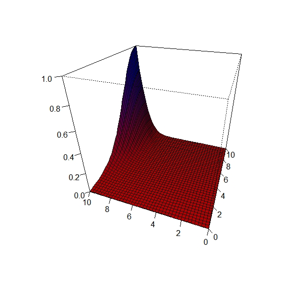
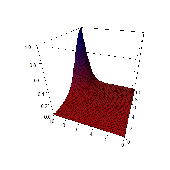
Figure 1: The joint cdf of $M(n)$ and $M_{u}(n)$ as given by (2.18) with
$F=U[0,a]$, $G=U[0,10]$, $p=0.7$. Left to right: $a=15,10,5$.

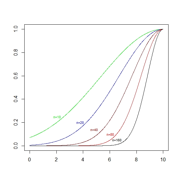
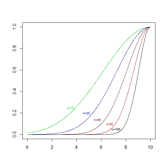
Figure 2: The cdf of $M_{u}(n)$ as given by (2.20) with $F=U[0,a]$, $G=U[0,10]$, $p=0.7$. Left to right: $a=15,10,5$.

Figure 3: The cdf of $M(n)$ as given by (2.22) with $F=U[0,a]$, $G=U[0,10]$, $p=0.7$. Left to right: $a=15,10,5$.

Figure 4: The cdf of $M(n)-M_{u}(n)$ as given by (2.23) with $F=$U[0, a$]$, $G=U[0,10]$, $p=0.7$. Left to right: $a=15,10,5$.

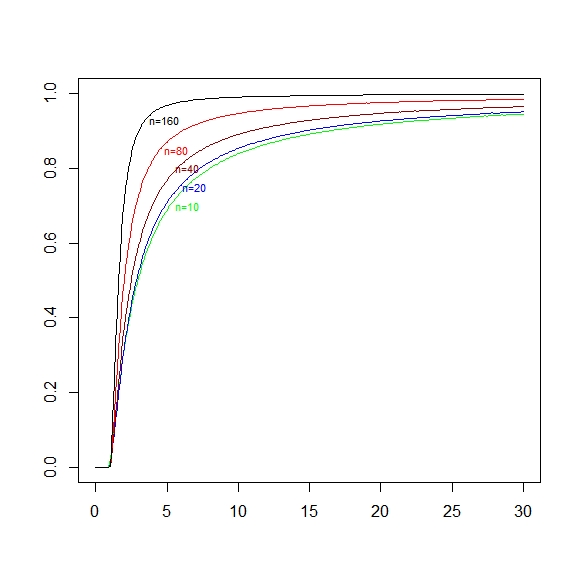
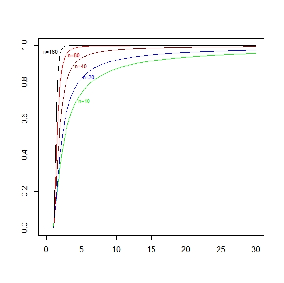
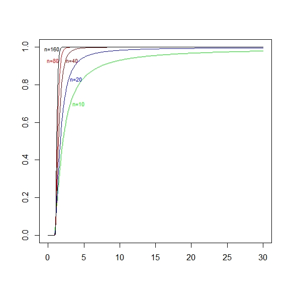
Figure 5: The cdf of $M(n)/M_{u}(n)$ (conditional on $M_{u}(n)>0$) as given by (2.26) with $F=$Exp($\lambda=0.0802$), $G=U[0,10]$, $p=0.7$.

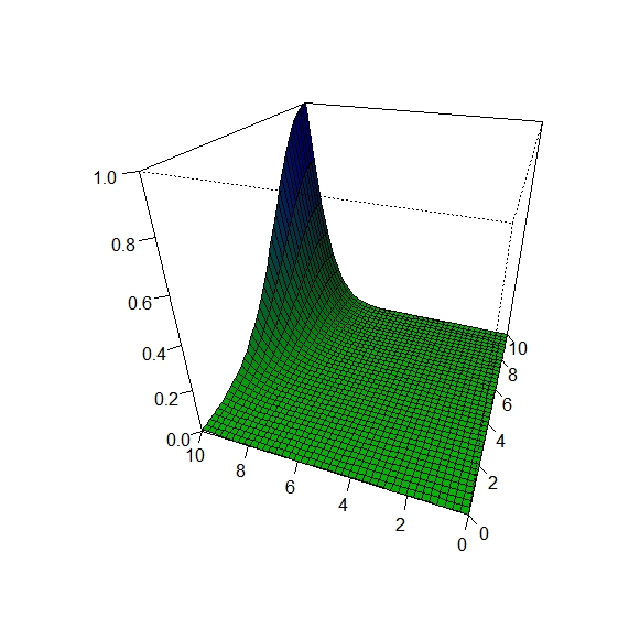
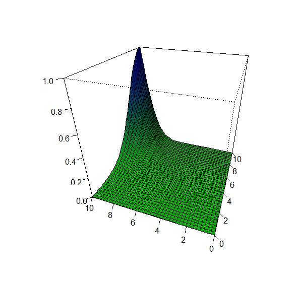
Figure 6: The joint cdf of $M(n)$ and $M_{u}(n)$ as given by (2.18) with $F=U[0,a]$, $G=U[0,10]$, $n=20$. Left to right: $p=0.33,0.66,1$. Top to bottom: $a=15,10,5$.

Figure 7: The cdf of $M_{u}(n)$ as given by (2.20) with $F=U[0,a]$, $G=U[0,10]$. Left to right: $p=0.33,0.66,1$. Top to bottom: $a=15,10,5$.

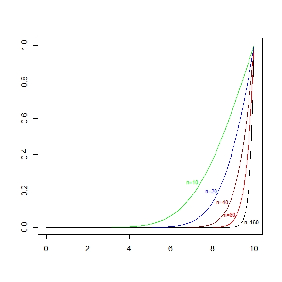
Figure 8: The cdf of $M(n)$ as given by (2.22) with $F=U[0,a]$, $G=U[0,10]$. Left to right: $p=0.33,0.66,1$. Top to bottom: $a=15,10,5$.

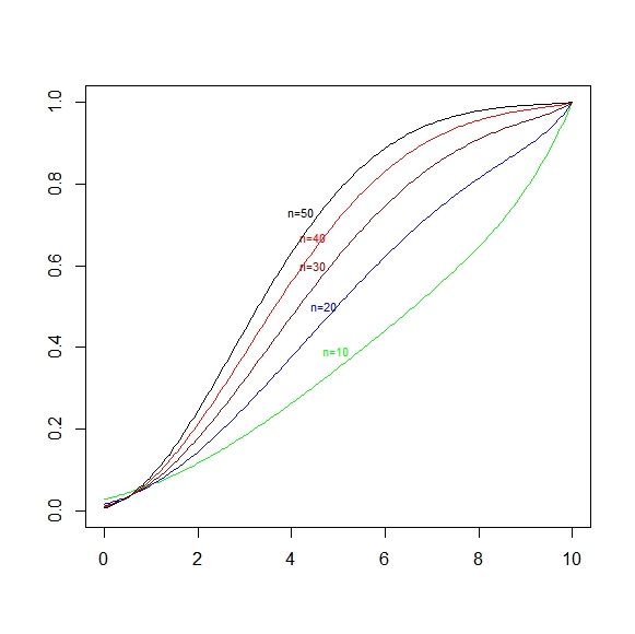
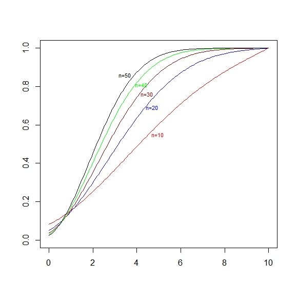
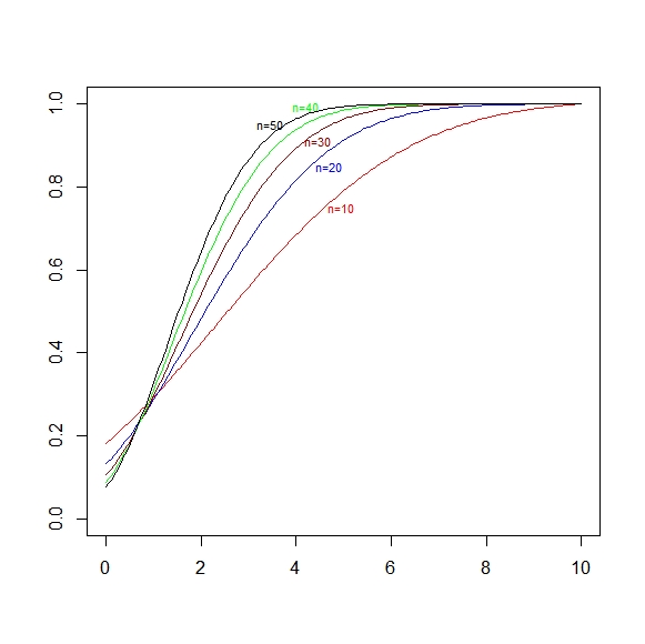
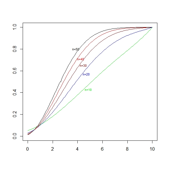
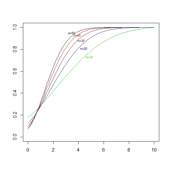
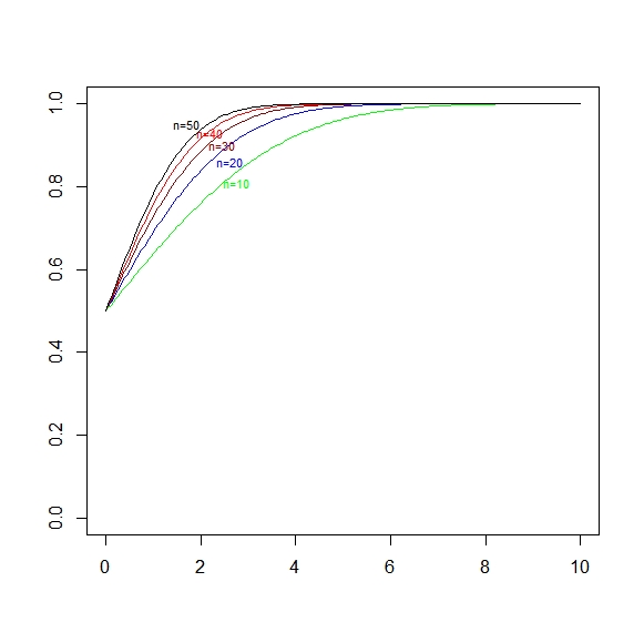
Figure 9: The cdf of $M(n)-M_{u}(n)$ as given by (2.23) with $F=U[0,a]$, $G=U[0,10]$. Left to right: $p=0.33,0.66,1$. Top to bottom: $a=15,10,5$.

References

- [1] Amico, M. and Van Keilegom, I. (2018) Cure models in survival analysis. Annual Review of Statistics and Its Application, 5, 311–342.
- [2] Escobar-Bach, M., Maller, R.A., Van Keilegom, I. and Zhao, M. (2020) Estimation of the cure rate for distributions in the Gumbel maximum domain of attraction under insufficient follow-up. Biometrika, to appear.
- [3] R.D. Gill. Censoring and stochastic integrals. Mathematical Centre Tracts, 124, Amsterdam: Mathematisch Centrum, 1980.
- [4] Goldman, A. (1984) Survivorship analysis when cure is a possibility: A Monte Carlo study. Stat. Med., 3, 153–163.
- [5] Goldman, A. (1991) The cure model and time confounded risk in the analysis of survival and other timed events. J. Clinical Epidemiology, 44, 1327–1340.
- [6] de Haan, L. and Ferreira, A. (2006) Extreme Value Theory. Springer, New York.
- [7] Kaplan, E.L. and Meier, P. (1958) Nonparametric estimation from incomplete observations. J. Amer. Statist. Assoc., 53, 457–481.
- [8] Liu, J., Lichtenberg, T., Hoadley, K.A., Poisson, L.M., Lazar, A.J., Cherniack, A.D.. Kovatich, A.J., Benz, C.C., Levine, D.A., Lee, A.V., Omberg, L., Wolf, D.M., Shriver, C.D., Thorsson, V. and Hu, H. (2018) An integrated TCGA pan-cancer clinical data resource to drive high-quality survival outcome analytics, Cell, 173(2), 400–416.
- [9] Maller, R.A. and Zhou, X. (1996) Survival Analysis with Long Term Survivors. Wiley, Chichester.
- [10] Maller, R.A. and Resnick, S.I. (2020) Extremes of censored and uncensored lifetimes in survival data. Under revision for Extremes.
- [11] Maller, R.A., Resnick, S.I. and Shemehsavar, S. (2020) Splitting the sample at the largest uncensored observation. arXiv:2103.01337
- [12] Othus, M., Barlogie, B., LeBlanc, M.L, and Crowley, J.J. (2012) Cure models as a useful statistical tool for analyzing survival. Clinical Cancer Research, 18, 311–342.
- [13] Othus, M., Bansal A., Erba, H., Ramsey, S. (2020) Bias in mean survival from fitting cure models with limited follow-up. Value in Health, 23, 1034–1039.
- [14] Peng, Y. and Taylor, J.M.G. (2014) Cure models. In: Klein, J., van Houwelingen, H., Ibrahim, J.G., and Scheike, T.H., Eds, Handbook of Survival Analysis, Handbooks of Modern Statistical Methods series, Chapter 6. Chapman & Hall, Boca Raton, FL, USA., 113–134.
- [15] Resnick, S.I. (2008) Extreme Values, Regular Variation and Point Processes. Springer, New York. Reprint of the 1987 original.
- [16] Shen, Pao-sheng (2000) Testing for sufficient follow-up in survival data. Statistics & Probability Letters, 49, 313–322.
- [17] F. Taweab and N. A. Ibrahim (2014) Cure rate models: a review of recent progress with a study of change-point cure models when cured is partially known. J. Appl. Sci., 14, 609–616.