Reeb flows transverse to foliations

Abstract.

Let $\mathcal{F}$ be a co-oriented $C^{2}$ foliation on a closed, oriented 3-manifold. We show that $T\mathcal{F}$ can be perturbed to a contact structure with Reeb flow transverse to $\mathcal{F}$ if and only if $\mathcal{F}$ does not support an invariant transverse measure. The resulting Reeb flow has no contractible orbits. This answers a question of Colin and Honda. The main technical tool in our proof is leafwise Brownian motion which we use to construct good transverse measures for $\mathcal{F}$; this gives a new perspective on the Eliashberg–Thurston theorem.

1. Introduction

In their seminal work [EET98], Eliashberg and Thurston proved that a $C^{2}$ foliation of a closed, oriented 3-manifold not homeomorphic to $S^{1}\times S^{2}$ may be $C^{0}$ approximated by positive or negative contact structures. When the foliation is taut, the approximating contact structures are universally tight and weakly symplectically fillable. This theorem, along with its subsequent generalizations [KR17, Bow16a], serves as a bridge between contact topology and the theory of foliations. In one direction, one can export genus detection results from Gabai’s theory of sutured manifolds to the world of Floer homology [Gab83, OS04]. In the other direction, a uniqueness result of Vogel for the approximating contact structure implies that invariants of the approximating contact structure become invariants of the deformation class of the foliation [Vog16, Bow16b].

Colin and Honda asked when the approximating contact structure can be chosen so that its Reeb flow is transverse to the foliation. When this is the case, the foliation can be used to control the Reeb dynamics. In particular, a transverse Reeb flow can have no contractible Reeb orbits. A contact form with this property is called hypertight. The hypertight condition is useful for defining and computing pseudo-holomorphic curve invariants. A motivating example for us is cylindrical contact homology, an invariant of contact structures that is well defined when the contact structure supports at least one hypertight contact form [BH18].

Colin and Honda constructed such transverse Reeb flows for sutured hierarchies [CH05]. They recently extended their methods to finite depth foliations on closed 3-manifolds [CH18]. In this setting, although the Reeb flow cannot be made transverse to the closed leaf, it is transverse to a related essential lamination and hence has no contractible orbits. The goal of the present paper is to give a complete answer to the existence question for transverse Reeb flows for all $C^{2}$ foliations.

A closed leaf is an obstruction to a transverse Reeb flow. Suppose that $\Sigma$ is a closed, oriented surface and $\alpha$ is the 1-form representing a contact structure $\xi$. By Stokes’ theorem, $\int_{\Sigma}d\alpha=0$ and it follows that $d\alpha=0$ at some point on $\Sigma$. The Reeb flow must be tangent to $\Sigma$ at this point. In particular, this implies that foliations with transverse Reeb flows have no compact leaves, and hence are taut.

More generally, suppose that $M$ is a closed, oriented 3-manifold with a co-orientable foliation $\mathcal{F}$ which supports an invariant transverse measure (possibly not of full support). Then $M$ has a closed 2-current $\Sigma$ tangent to $\mathcal{F}$. The argument above still applies to show that $\mathcal{F}$ does not have a transverse Reeb flow.

We prove that for $C^{2}$ foliations, this is the only obstruction.

Theorem 1.

Let $\mathcal{F}$ be a co-orientable $C^{2}$ foliation on a closed, oriented 3-manifold $M$. Then $T\mathcal{F}$ can be perturbed to a contact structure with Reeb flow transverse to $\mathcal{F}$ if and only if $\mathcal{F}$ does not support an invariant transverse measure.

When $\mathcal{F}$ is taut, an invariant transverse measure gives rise to a nontrivial class in $H^{1}(M,\mathbb{R})$. Therefore, we have the following corollary (c.f. Conjecture 1.5 from [CH05]):

Corollary 1.

If $M$ is a closed, oriented 3-manifold with a co-oriented $C^{2}$ taut foliation and $M\ncong S^{1}\times S^{2}$, then $M$ supports a hypertight contact structure.

Proof.

If $H^{1}(M,\mathbb{R})=0$, then the foliation has no invariant transverse measure and 1 applies. Otherwise, $M$ supports a finite depth taut foliation. In this case, Theorem 3.14 of [CH18] gives the desired hypertight contact structure. ∎

One should think of invariant transverse measures as exceptional. In fact, under some conditions, it follows from a result of Bonatti–Firmo that non-existence of invariant transverse measures is generic for $C^{\infty}$ foliations.

Corollary 2.

Suppose that $M$ a closed, oriented, atoroidal 3-manifold. Then any $C^{\infty}$ taut foliation on $M$ is $C^{0}$ close to a hypertight contact structure.

Corollary 3.

Cylindrical contact homology is an invariant of the taut deformation class of $C^{\infty}$ taut foliations on closed, oriented, atoroidal 3-manifolds.

We defer explanations of the last two corollaries to Section 6.

Our method contrasts with prior constructions of contact approximations. The strategy of Eliashberg and Thurston begins with identifying some closed curves in leaves of $\mathcal{F}$ with attracting holonomy. They produce a contact perturbation in the neighbourhood of these curves, and then “flow” the contactness to the rest of the 3-manifold. It is not clear how to control the Reeb vector field during this flow operation. In the case of sutured hierarchies, Colin and Honda give an explicit inductive construction of the contact perturbation. At each step of the sutured hierarchy, they can ensure that the Reeb flow has a good standard form near the boundary compatible with the sutures.

Our construction begins with an arbitrary transverse measure for $\mathcal{F}$ and smooths it out by logarithmic diffusion. This process is similar to the leafwise heat flow studied by Garnett [Gar83]. The advantage of our diffusion process is that we can show that in finite time, the transverse measure becomes log superharmonic. Roughly speaking, this means that the transverse distance between two nearby leaves is the exponential of a superharmonic function. This gives a global picture of the holonomy of $\mathcal{F}$. Finally, we show that there is a canonical way to deform a log superharmonic transverse measure into a contact structure. Since this perturbation is done in one shot, we have full control over the Reeb flow.

2. Examples

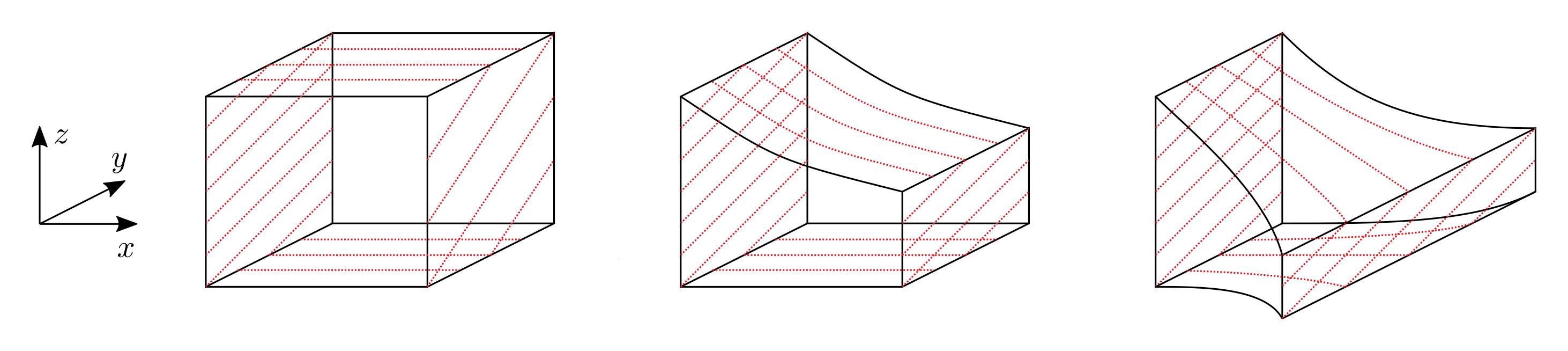
Figure 1. Here are three boxes, each equipped with both a product foliation transverse to the $z$ direction and an approximating contact structure. The top and bottom faces of each box are leaves. The red dotted lines show the characteristic foliation of the contact structure on some of the boxes’ faces. Observe that in the first box, the slope of the characteristic foliation on the left face is greater than the slope on the right face. These ever increasing slopes are unsustainable in a closed manifold. The second and third boxes (corresponding with 1 and 2) are diffeomorphic to the first, but we have introduced some contraction of the leaves of the foliation. Now the slopes on the left and right faces can be made identical, facilitating gluing up to a closed manifold.

Example 1 (creating contact regions using holonomy).

Consider $\mathbb{R}^{3}$ foliated by planes $z=\text{const}$ and endowed with the Riemannian metric $g=dx^{2}+dy^{2}+2^{-2x}dz^{2}$. This is a local model for a foliation with holonomy. One may produce a contact structure by rotating the tangent planes to the foliation by a Riemannian angle of $\varepsilon$ around an axis parallel to the $x$ axis. Any line parallel to the $x$ axis is a Legendrian. Travelling along such a Legendrian in the positive $x$ direction, the Riemannian angles are constant, so the Euclidean angles are increasing. This twisting of contact planes along a Legendrian is the hallmark of a contact structure.

In equations, the contact form is $\alpha:=2^{-x}dz+\varepsilon dy$ and

$$d\alpha=-2^{-x}dx\wedge dz$$

In this case, the Reeb flow is not transverse to the foliation but points in the $y$ direction. This construction may equally well be done in the quotient of $\mathbb{R}^{3}$ by the isometry $(x,y,z)\mapsto(x+1,y,2z)$. Here we have seen the general rule that “Legendrians (in the characteristic foliation on a leaf) flow in the direction of contracting holonomy”.

Example 2 (Anosov flows).

1 can be modified so that the Reeb flow is transverse to the leaves. We make the Legendrian flow Anosov, i.e. spreading out in the $y$-direction as well as contracting in the $z$-direction. The relevant metric is $g=dx^{2}+2^{2x}dy^{2}+2^{-2x}dz^{2}$.

It is instructive to write this example in different coordinates. Let $\mathbb{H}=\left\{\,(x,y)\,\mid\,y\geq 0\,\right\}$ be the upper half plane. Let $f(x,y)=y$. Give $\mathbb{H}\times\mathbb{R}$ coordinates $x,y,t$. The 1-form $fdt$ defines the horizontal foliation and is an example of a harmonic transverse measure. The Anosov flow is parallel to the $y$ axis. The 1-form $\alpha=fdt-\varepsilon\star d\log f$ is a contact perturbation. Indeed,

$$\alpha =ydt+\varepsilon\frac{1}{y}dx$$

$$\alpha\wedge d\alpha =\varepsilon(2\frac{1}{y}dx\wedge dy\wedge dt)+O(\varepsilon^{2})$$

This time, the Reeb flow is transverse to the foliation since $d\alpha$ evaluates positively on $\mathcal{F}$. The moral here is that “spreading of the Legendrians” in the characteristic foliation can contribute to contactness, and also help to make the Reeb flow transverse to the foliation.

Example 3 (a coarsely harmonic transverse measure).

Here is an example of a foliation with holonomy that one can keep in mind while reading the rest of the paper. Let $P$ be a pair of pants with boundary components $a$,$b$, and $c$. Let $\varphi$ be a diffeomorphism of $P$ exchanging $b$ and $c$. Let $M^{\circ}$ be the mapping torus of $\varphi$. The manifold $M^{\circ}$ has a foliation by parallel copies of $P$. It has two toroidal boundary components, each with a horizontal foliation and one “twice as long” as the other. Glue these boundary components together by a map $\theta\mapsto 2\theta$, where $\theta$ parameterizes the direction transverse to $P$. Call the resulting foliated manifold $M$.

Now let $f$ be a function on $P$ which takes the value $1$ on $b$ and $c$ and the value $2$ on $a$. We can further arrange that $f$ is invariant under $\varphi$ and has only a single critical point. Then $f$ pulls back to $M^{\circ}$. After some smoothing near the cuffs, the 1-form $f\,d\theta$ is a smooth transverse measure on $M$. With respect to this transverse measure, the manifold has contracting holonomy along paths from $a$ to $b$ or $a$ to $c$.

Example 4 (sutured manifold).

The foliation in 3 has every leaf dense, but we will also need to consider foliations whose leaves accumulate on sublaminations. The example to keep in mind is a taut sutured manifold. One of the simplest sutured manifolds is the solid torus $T_{n}$ with $2n$ longitudinal sutures, $n\geq 2$. It is foliated by a stack of monkey saddles, each of which accumulates on the boundary leaves. For a natural choice of Riemannian metric, the foliation has contracting holonomy along every path to infinity in a leaf. This foliation supports a contact structure whose characteristic foliation on each leaf consists of radial lines emanating from a single elliptic singularity to infinity. The Reeb flow has a single periodic orbit along the core of the solid torus; every other orbit enters along a positively oriented boundary leaf and leaves along a negatively oriented one. See Fig. 2

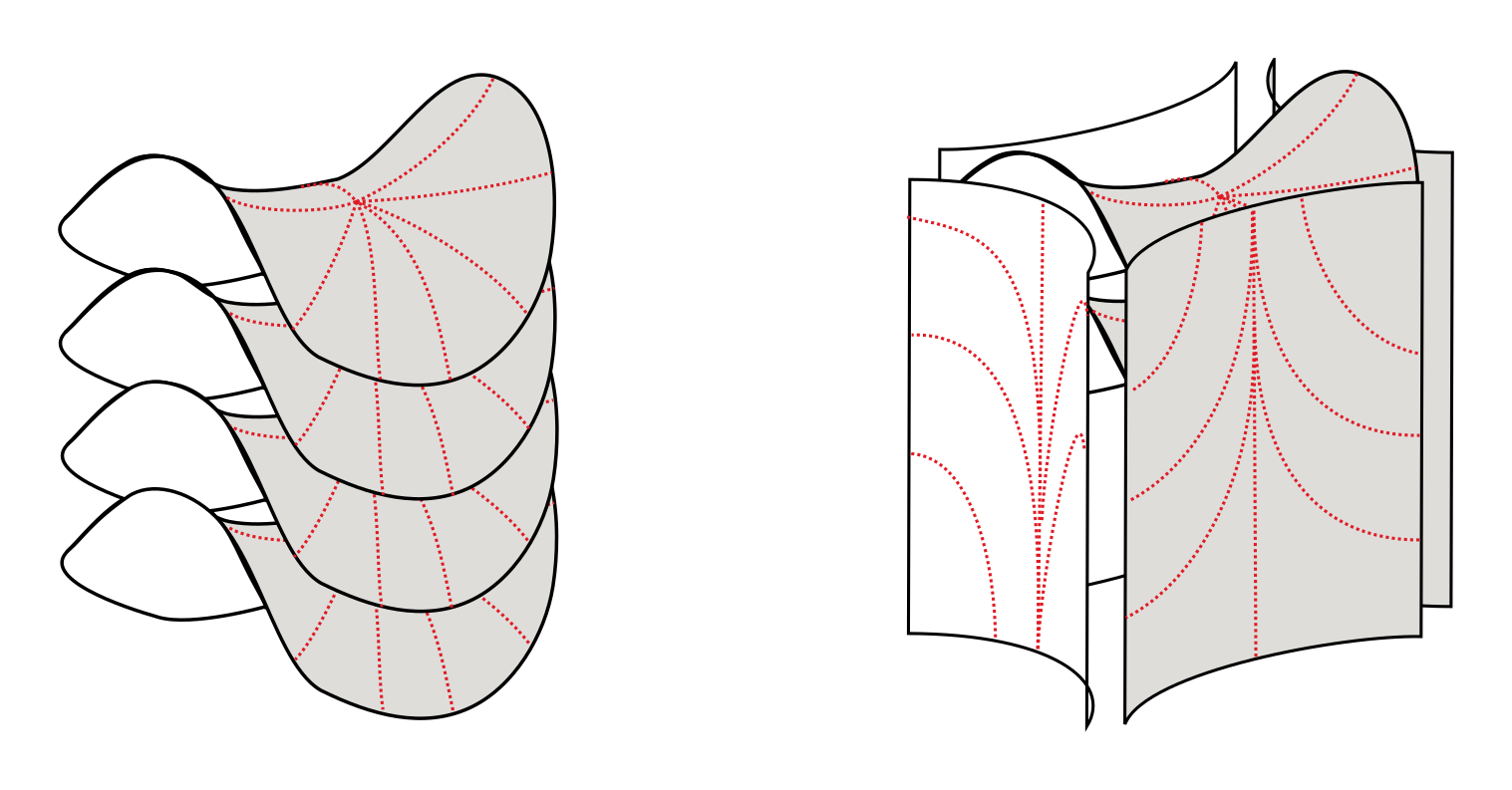
Figure 2. This is a foliation by saddles of the solid torus with four longitudinal sutures. The $S^{1}$ direction is vertical. The limiting annular boundary leaves are added on the right. The red dotted lines denote the characteristic foliation of an approximating contact structure.

3. Preliminaries

Unless stated otherwise, all manifolds are closed oriented and all foliations are oriented and co-oriented.

3.1. Foliations and their regularity

A foliation is a decomposition of a 3-manifold into surfaces, locally modelled on $\mathbb{R}^{2}\times\mathbb{R}$. A foliation is specified by a covering of $M$ by charts such that their transition maps preserve the decomposition of $\mathbb{R}^{3}$ into horizontal planes. The surfaces in the decomposition are called leaves. A foliation is oriented if the transition maps preserve the orientations of the leaves and co-oriented if the transition maps preserve the orientation of the transverse $\mathbb{R}$ factor.

For $k\geq l$, we say that a foliation is $C^{k,l}$ if the mixed partial derivatives of the transition maps up to order $l$ in the transverse direction and up to order $k$ in total exist and are continuous. Calegari showed that the tangential regularity (i.e. the value of $k$) of a foliation can always be improved to $\infty$ by a topological isotopy. However, it might not be possible to improve the transverse regularity class of a foliation; the holonomy maps of a $C^{k,0}$ foliation are $C^{0}$ functions which might not be conjugate to smooth functions. When we say that a foliation is $C^{k}$, we mean that it is $C^{\infty,k}$. We will also use the notation $C^{k,l}$ to denote the regularity class of functions on $M$.

3.2. Transverse measures

A transverse measure is an assignment of a positive real number to each arc positively transverse to $\mathcal{F}$. We ask that the assignment be countably additive under concatenation of arcs. An invariant transverse measure is one with respect to which the length of a transverse arc does not change under any homotopy keeping its endpoints on the same pair of leaves.

A compact leaf $\lambda$ gives rise to an invariant transverse measure which assigns to each transverse arc the number of intersections with $\lambda$. We will generally be concerned with smooth transverse measures of full support. Such a transverse measure $\tau$ can be encoded as a nowhere-vanishing $C^{k,l}$ 1-form with $\ker(\tau)=T\mathcal{F}$.

3.3. Taut foliations

A foliation $\mathcal{F}$ on a 3-manifold $M$ is taut if any of the following equivalent conditions hold:

1. For each point $x\in M$, there is a closed curve transverse to $\mathcal{F}$ passing through $x$.

2. There is a volume preserving flow transverse to $\mathcal{F}$.

3. There is a closed 2-form $\omega$ evaluating positively on $T\mathcal{F}$.

Taut foliations enjoy a number of good properties.

1. Loops transverse to $\mathcal{F}$ are not contractible.

2. Leaves of $\mathcal{F}$ are $\pi_{1}$-injective.

If we exclude the exceptional case $M\cong S^{1}\times S^{2}$ we can say more.

1. $M$ is irreducible.

2. The universal cover $\widetilde{M}$ is $\mathbb{R}^{3}$.

3. Leaves of $\widetilde{F}$ are properly embedded planes in $\widetilde{M}$.

If a foliation has no compact leaves, then it is taut.

3.4. Contact structures

A contact structure on an oriented 3-manifold $M$ is a plane field $\xi$ such that there exists a 1-form $\alpha$ with $\xi=\ker(\alpha)$ and $\alpha\wedge d\alpha>0$. The Reeb flow of $\alpha$ is a vector field $R$ uniquely defined by the following properties:

$$d\alpha(R,-) =0$$

$$\alpha(R) =1$$

The Reeb flow is always transverse to $\xi$, and moreover is transverse to any tangent plane on which $d\alpha>0$. The Reeb flow preserves $\alpha$. In particular, it preserves the volume form $\alpha\wedge d\alpha$. Compare this with the second definition of taut foliation above; it follows that a foliation with a transverse Reeb flow is taut.

Given a surface $\Sigma\subset M$, the characteristic foliation of $\xi$ on $\Sigma$ is the singular codimension 1 foliation on $\Sigma$ defined by the intersection of $\xi$ with $\Sigma$.

3.5. Holonomy

Let $M$ be an oriented 3-manifold with a taut, co-oriented $C^{2}$ foliation, $\mathcal{F}$. Choose a background Riemannian metric for $M$.

A transversal to $\mathcal{F}$ is an closed arc transverse to $\mathcal{F}$ making a Riemannian angle of at least $\pi/4$ with $\mathcal{F}$. The precise value of this bound is unimportant; it is simply necessary that we be able to uniformly compare transversals to vectors in $T^{\perp}\mathcal{F}$.

Let $\gamma\colon[0,T]\to M$ be a path which is tangent to $\mathcal{F}$ and supported in a single foliation chart $U$. Let $I_{0},I_{T}\subset U$ be transversals to $\mathcal{F}$ through $\gamma(0),\gamma(T)$ respectively. We define the holonomy map $h_{\gamma}\colon I_{0}\to I_{T}$ to be a map preserving the transverse coordinate of the foliation chart. The holonomy map can be defined for arbitrary paths $\gamma$ tangent to $\mathcal{F}$ by composing holonomy maps for short subpaths. As $\gamma$ grows in length, the domain of $h_{\gamma}$ tends to shrink.

Since $\mathcal{F}$ is $C^{2}$, the infinitesimal holonomy map $h^{\prime}_{\gamma}\colon T^{\perp}_{\gamma(0)}\mathcal{F}\to T^{\perp}_{\gamma(T)}\mathcal{F}$ exists. Suppose now that $\mathcal{F}$ is equipped with a smooth transverse measure $\tau$, encoded as a 1-form with $\ker(\tau)=T\mathcal{F}$. Then we define

$$\left|h_{\gamma}^{\prime}\right|_{\tau}=\frac{\tau(h_{\gamma}^{\prime}(v))}{\tau(v)}$$

where $v$ is any non-zero vector in $T^{\perp}_{\gamma(0)}\mathcal{F}$. In other words, $\left|h_{\gamma}^{\prime}\right|_{\tau}$ is the factor by which holonomy along $\gamma$ stretches $\tau$-lengths. Note that the dependence on $\tau$ is weak; given any two transverse measures $\tau,\mu$, the norms $|\cdot|_{\mu}$ and $|\cdot|_{\tau}$ differ by at most an absolute constant factor.

Given a leaf $\lambda$ and a basepoint $b$ in $\widetilde{\lambda}$, we define the Radon-Nikodym derivative of $\tau$, $f_{\tau,\lambda}\colon\widetilde{\lambda}\to\mathbb{R}$, by

$$f_{\tau,\lambda}(x)=\left|h_{\gamma}^{\prime}\right|_{\tau}$$

where $\gamma$ is a path in $\widetilde{\lambda}$ from $b$ to $x$, and $h_{\gamma}^{\prime}$ is the holonomy of $\widetilde{\mathcal{F}}$ along $\gamma$. One should think of $f_{\tau,\lambda}$ as the transverse distance to a nearby leaf as measured by $\tau$. We omit the basepoint from the notation, but one should remember that $f_{\tau,\lambda}$ is only defined up to a constant factor due to this ambiguity. When there is no danger of ambiguity, we abbreviate $f_{\tau,\lambda}$ to $f_{\tau}$.

A theme in what follows is that for the best transverse measures, $f_{\tau,\lambda}$ has no local minima. When $f_{tau,\lambda}$ is harmonic on each leaf $\widetilde{\lambda}$, $\tau$ is called a harmonic transverse measure. When $\log f_{\tau,\lambda}$ is superharmonic (resp. strictly superharmonic) on each leaf $\widetilde{\lambda}$, we say that $\tau$ is log superharmonic (resp. strictly log superharmonic). Since log is concave, every harmonic transverse measure is also log superharmonic.

While $f_{\tau}$ is defined on $\widetilde{M}$ and makes sense only up to constant factors for each leaf, several related objects descend to $M$. The 1-form $d\log f_{\tau}$ is a well-defined section of $T^{*}\mathcal{F}$. It measures the infinitesimal rate of contraction or expansion of leaves in directions tangent to $\mathcal{F}$. The function $\Delta\log f_{\tau}$, where $\Delta$ denotes the leafwise Laplacian operator, is consequently also defined on $M$. Finally, the leafwise level sets of $f_{\tau}$ descend to a singular codimension 2 foliation on $M$.

3.6. Leafwise Brownian motion and diffusion

Fix a background Riemannian metric. Let $\lambda$ be the leaf of $\mathcal{F}$ containing a point $x$. Let $\Gamma_{x}$ be the space of continuous paths in $\lambda$ starting at $x$. We define $W_{x}$ to be the Wiener measure on paths beginning from a point $x$. For any function $g$ on $M$, we define its time $t$ diffusion $D^{t}(g)$ by

$$D^{t}(g)(x)=\operatorname{\mathbb{E}}_{\gamma\sim W_{x}}\left[g(\gamma(t))\right].$$

In the course of the proof, we will define another diffusion operator $\mathcal{D}_{T,R,S}$ acting on transverse measures. These two operators should not be confused.

3.7. Assorted notation

Given points $x,y$ on the universal cover of a leaf $\lambda$, let $d(x,y)$ denote the leafwise Riemannian distance between $x$ and $y$ in $\widetilde{\lambda}$. We denote by $\star_{2}$ the leafwise Hodge star operator acting on $\Lambda^{*}(T^{*}F)$.

4. Existence of transverse Reeb flows

In this section, we prove 1. Let $M$ be a closed, oriented 3-manifold with a co-oriented $C^{2}$ foliation $\mathcal{F}$. If $\mathcal{F}$ supports an invariant transverse measure, then as discussed in the introduction, there is no Reeb flow transverse to $\mathcal{F}$.

For the rest of the section, we consider the case that $\mathcal{F}$ supports no transverse invariant measure. In particular, this implies that $\mathcal{F}$ is taut. Our goal is to construct a contact perturbation of $T\mathcal{F}$ with Reeb flow transverse to $\mathcal{F}$.

4.1. Structure theorem for $C^{2}$ foliations

Deroin and Kleptsyn gave a precise picture of the long term dynamics of leafwise Brownian motion and the holonomy along such paths. We reproduce their main theorem here for reference:

Theorem 2 ([DK07]).

Let $\mathcal{F}$ be a $C^{1}$ foliation of a closed 3-manifold $M$. Then either $\mathcal{F}$ supports an invariant transverse measure, or $\mathcal{F}$ has a finite number of minimal sets $\mathcal{M}_{1},\dots,\mathcal{M}_{k}$ equipped with probability measures $\mu_{1},\dots,\mu_{k}$, and there exists a real $\kappa>0$ such that:

1. Contraction. For every point $x\in M$ and almost every leafwise Brownian path $\gamma$ starting at $x$, there is a transversal $I_{\gamma}$ at $x$ and a constant $C_{\lambda}>0$, such that for every $t>0$, the holonomy map $h_{\gamma|_{[0,t]}}$ is defined on $I_{\gamma}$ and

   $$|h_{\gamma|_{[0,t]}}(I_{\gamma})|\leq C_{\gamma}\exp(-\kappa t)$$

2. Distribution. For every point $x\in M$ and almost every leafwise Brownian path $\gamma$ starting at $x$, the path $\gamma$ tends to one of the minimal sets, $\mathcal{M}_{j}$, and is distributed with respect to $\mu_{j}$, in the sense that

   $$\lim_{t\to\infty}\frac{1}{t}\gamma_{*}\operatorname{leb}_{[0,t]}=\mu_{j}$$

   where $\operatorname{leb}_{[0,t]}$ is the standard Lebesgue measure on $[0,t]$.

3. Attraction. The probability $p_{j}(x)$ that a leafwise Brownian path starting at a point $x$ of $M$ tends to $\mathcal{M}_{j}$ is a continuous leafwise harmonic function (which equals 1 on $\mathcal{M}_{j}$).

4. Diffusion. When $t$ goes to infinity, the diffusions $D^{t}$ of a continuous function $f:M\to\mathbb{R}$ converge uniformly to the function $\sum_{j}c_{j}p_{j}$, where $c_{j}=\int f\,d\mu_{j}$. In particular, the functions $p_{j}$ form a base in the space of continuous leafwise harmonic functions.

Remark 1.

It might be surprising that holonomy is contracting in almost every direction. It is instructive to verify 2 for the foliation in 3. A point undertaking Brownian motion in a pair of pants in $\mathcal{F}$ has three options for a cuff through which to exit. Two of these options have contracting holonomy and one has expanding holonomy. Therefore, with overwhelming probability, holonomy along leafwise Brownian path is exponentially contracting. In this case, there is only one minimal set $\mathcal{M}_{1}=M$. The ergodicity statement reduces to the ergodicity of the associated dynamical system on the $S^{1}$ factor transverse to the leaves of $M^{\circ}$ defined by

$$z\mapsto\begin{cases}\sqrt{z},&\text{with probability 1/2}\\ -\sqrt{z},&\text{with probability 1/2}\end{cases}$$

where $S^{1}$ is identified with the unit circle in $\mathbb{C}$.

Remark 2.

The non-existence of an invariant transverse measure is equivalent to an isoperimetric inequality for subsurfaces of leaves, i.e. the existence of a Cheeger constant $h>0$ such that $\frac{\left|\partial S\right|}{\left|S\right|}\geq h$ for any compact subsurface $S$ of the leaves of $\mathcal{F}$. Therefore, the theorem above may be regarded as an analogue of the Cheeger inequality for foliations: if $\mathcal{F}$ has a nonzero Cheeger constant, then leafwise random walks converge quickly to a stationary distribution.

Our foliations are $C^{2}$, so we can upgrade the contraction result to an infinitesimal version:

Proposition 1.

Let $\mathcal{F}$ be a $C^{2}$ foliation of a closed 3-manifold $M$. Suppose further that $\mathcal{F}$ does not support an invariant transverse measure. Then there exists a real number $\kappa>0$ such that for every point $x\in M$ and almost every leafwise Brownian path $\gamma$ starting at $x$, there is a constant $C_{\gamma}>0$ such that for every time $t>0$, the holonomy map $h_{\gamma|_{[0,t]}}$ satisfies

$$\left|h_{\gamma|_{[0,t]}}^{\prime}\right|\leq C_{\gamma}\exp(-\kappa t)$$

Remark 3.

We don’t need to specify a transverse measure for the norm $\left|\cdot\right|$ since $C_{\gamma}$ can absorb constant factors.

Proof.

Given an orientation preserving homeomorphism $g$ between two intervals $I_{0}$ and $I_{1}$, we define the distortion of $g$ by

$$\operatorname{distortion}(g)=\sup_{a,b,c,d\in I_{0}}\frac{a-b}{c-d}\bigg{/}\frac{g(a)-g(b)}{g(c)-g(d)}.$$

The distortion is equal to 1 if and only if $g$ is linear. It is submultiplicative with respect to composition of functions. If $g$ is $C^{2}$, then there is a bound on the distortion in terms of $g^{\prime\prime}$:

$$\operatorname{distortion}(g) =\frac{\sup_{x\in I_{0}}g^{\prime}(x)}{\inf_{x\in I_{0}}g^{\prime}(x)}$$ (1)

$$\leq 1+\frac{\left|I_{0}\right|\sup_{x\in I_{0}}{\left|g^{\prime\prime}(x)\right|}}{\inf_{x\in I_{0}}\left|g^{\prime}(x)\right|}$$ (2)

Let $\varepsilon$ be small enough that holonomy maps over leafwise paths of length $\leq 1$ are defined on all transversals of length $\leq\varepsilon$. Let $A$ be an upper bound for the quotient $\frac{\sup_{x\in I_{0}}\left|g^{\prime\prime}(x)\right|}{\inf_{x\in I_{0}}\left|g^{\prime}(x)\right|}$ over all holonomy maps $g$ for transversals of length $\leq\varepsilon$ along paths of length $\leq 1$.

Let us now consider a leafwise Brownian path $\gamma$ starting at a point $x\in M$. By 2, we may choose a short transversal $I_{\gamma}$ through $x$ such that holonomy of $I_{\gamma}$ along $\gamma$ exists for all time, and moreover that there exists a constant $C_{\gamma}$ permitting the inequality

$$\left|h_{\gamma\mid_{[0,t]}}(I_{\gamma})\right|<C_{\gamma}\cdot\exp(-\kappa t)<\varepsilon$$ (3)

for all $t>0$. Break the holonomy $h_{\gamma|_{[0,t]}}$ into a composition

$$h_{\gamma|_{[0,t]}}=h_{\gamma|_{[t-1,t]}}\circ\dots\circ h_{\gamma|_{[1,2]}}\circ h_{\gamma|_{[0,1]}}.$$

Let $V(i)$ be the Riemannian leafwise distance between $\gamma(i)$ and $\gamma(i+1)$. Since distortion is submultiplicative, we have

$$\operatorname{distortion}(h_{\gamma|_{[0,t]}}) <\prod_{i=0}^{t-1}\operatorname{distortion}(h_{\gamma|_{[i,i+1]}})$$ (4)

$$<\prod_{i=0}^{t-1}\left(1+A\left|h_{\gamma\mid_{[0,i]}}(I_{\gamma})\right|\right)^{\lceil V_{i}\rceil}$$ (5)

$$<\prod_{i=0}^{t-1}(1+A\cdot C_{\gamma}\exp(-\kappa i))^{\lceil V_{i}\rceil}$$ (6)

In Eq. 5, we used the fact that $\gamma|_{[i,i+1]}$ is homotopic rel. endpoints to the concatenation of at most $\lceil V_{i}\rceil$ paths of length at most 1 and invoked Eq. 2. Since $V_{i}$ has finite moments, the last expression is almost surely bounded by a constant $B$ independent of $t$ with probability 1. Now we can estimate $h^{\prime}_{\gamma|_{[0,t]}}$ using our bound on the distortion of $h_{\gamma|_{[0,t]}}$ combined with the macroscopic bound given by 2:

$$\left|h^{\prime}_{\gamma|_{[0,t]}}\right| <B\left|h_{\gamma|_{[0,t]}}(I_{\gamma})\right|$$

$$<B\cdot C_{\gamma}\exp(-\kappa t)$$

∎

4.2. Logarithmic diffusion

In this subsection, $x$ will be a point in $M$ and $\lambda$ will be the leaf containing $x$. We will abbreviate $f_{\tau,\lambda}$ to $f_{\tau}$ when there is no danger of ambiguity. Let $W_{x}$ be the distribution of leafwise Brownian paths starting at a point $x$. Given a time $T>0$, we define a diffusion operator $\mathcal{D}_{T}$ acting on positive transverse measures by

$$\mathcal{D}_{T}(\tau)|_{x} =\exp\left(\operatorname{\mathbb{E}}_{\gamma\sim W_{x}}\left[\log\left|h^{\prime}_{\gamma|_{[0,T]}}\right|_{\tau}\right]\right)\tau|_{x}$$

where $\gamma$ is a leafwise Brownian path starting from $x$.

In other words, the $\mathcal{D}_{T}(\tau)$ length of an infinitesimal transverse arc through $x$ is the geometric mean of the $\tau$ lengths obtained by holonomy transport along time $T$ leafwise random walks. For an individual leaf $\lambda$, the function $\log f_{\tau,\lambda}$ on $\widetilde{\lambda}$ evolves according to the standard heat flow. If the geometric mean were to be replaced with an arithmetic mean, we would obtain the leafwise heat flow defined by Garnett [Gar83]. Unlike the heat flow operator, our diffusion operator does not conserve mass. Its advantage is that it gives greater weight to the well-behaved smaller holonomies, and therefore allows us to prove a quantitative convergence result.

The main result of this subsection is 2, which asserts that at some large but finite time $T$, the Radon-Nikodym derivatives of the diffused transverse measure are exponentials of strictly superharmonic functions. This implies, for example, that the distance to a nearby leaf, as measured by the diffused transverse measure, never has local minima.

As written, it is hard to prove any transverse regularity for the diffused measure. One cannot compare the diffused transverse measure at two nearby points on distinct leaves because holonomy of a transversal connecting these two points typically blows up in finite time along some long Brownian paths. We resolve this by introducing a cutoff function $\varphi_{R,S}$. We set

$$\mathcal{D}_{T,R,S}(\tau)|_{x}=\exp\left(\operatorname{\mathbb{E}}_{\gamma\sim W_{x}}\left[\log\left|h^{\prime}_{\gamma|_{[0,T]}}\right|_{\tau}\right]\varphi_{R,S}\left(x,\gamma(t_{\mathrm{far}})\right)\right)\tau|_{x}$$

where $t_{\mathrm{far}}\in[0,T]$ is the time minimizing $\varphi_{R,S}(x,\gamma(t_{\mathrm{far}}))$ and $\varphi_{R,S}(x,-)$ is a smooth cutoff function defined on $\widetilde{\lambda}$ satisfying the following conditions:

• $\varphi_{R,S}(x,y)=1$ when $d(x,y)<R$

• $\varphi_{R,S}(x,y)=0$ when $d(x,y)>SR$

• $\varphi$ has all derivatives bounded in absolute value by $\frac{10}{S}$

• The superlevel sets of $\varphi(x,-)$ on $\widetilde{\lambda}$ are topological disks.

The reader may now proceed to the proof of 2 and refer to the preceding technical lemmas as needed.

Lemma 1.

$\mathcal{D}_{T,R,S}(\tau)$ is $C^{\infty,1}$ for all $T,R,S$.

Proof.

This is where the cutoff comes in handy. Let $x$ be a point on a leaf $\lambda$. In $\widetilde{M}$, choose a neighbourhood $U$ of the radius $SR$ disk in $\widetilde{\lambda}$ centred at $x$ which is skinny enough in the transverse direction that it is foliated as a product. In a neighbourhood of $x$, the values of $\mathcal{D}_{T,R,S}(\tau)$ depend only on information in $U$. If we were to ignore the dependence of $t_{\mathrm{far}}$ on $\gamma$, then smoothness of $\mathcal{D}_{T,R,S}(\tau)$ would follow from standard results regarding the smoothness of heat kernels with respect to compact variations of the metric. The dependence of $t_{\mathrm{far}}$ on $\gamma$ can indeed be trivialized, as we now detail.

Suppose $x(\varepsilon)$ is a smooth path in $U$ with $x(0)=x$. To show that $\tau$ is once differentiable at $x$, we need to show that

$$\frac{\partial}{\partial\varepsilon}\mathcal{D}_{T,R,S}(\tau)(v)\mid_{x(\varepsilon)}$$

exists for any smooth vector field $v$.

Let $\widetilde{\lambda}_{\varepsilon}\subset U$ be the leaf containing $x(\varepsilon)$. Let $\psi_{\varepsilon}:\mathbb{R}^{2}\to\lambda_{\varepsilon}$ be a smooth family of diffeomorphisms parameterized by $\varepsilon$ such that $\psi_{\varepsilon}(0)=x(\varepsilon)$ and that $\psi_{\varepsilon}^{*}(\varphi(x(\varepsilon),-))$ is a standard, rotationally symmetric function on $\mathbb{R}^{2}$ independent of $\varepsilon$. Call this standard cutoff function $\varphi_{0}:\mathbb{R}^{2}\to\mathbb{R}$.

Let

$$g_{\varepsilon}=\psi_{\varepsilon}^{*}(g)$$

$$f^{\varepsilon}_{\tau}=\psi_{\varepsilon}^{*}(f_{\tau})$$

where $g$ is the Riemannian metric on $\widetilde{M}$. We resolve the scaling ambiguity of $f^{\varepsilon}_{\tau}$ by fixing $f^{\varepsilon}_{\tau}(x(\varepsilon))=\tau(v)$; this makes $f_{\tau}^{\varepsilon}$ a $C^{\infty,1}$ function on $\mathbb{R}^{2}\oplus\mathbb{R}$, where the $\mathbb{R}$ factor is parameterized by $\varepsilon$.

Let $W_{\mathbb{R}^{2}}$ be the distribution of Brownian paths in $\mathbb{R}^{2}$ starting from the origin. We can write $\mathcal{D}_{T,R,S}(\tau)$ in terms of Brownian motion on $\mathbb{R}^{2}$.

$$\mathcal{D}_{T,R,S}(\tau)(v)\mid_{x(\varepsilon)} =\exp\left(\operatorname{\mathbb{E}}_{\gamma\sim W_{x(\varepsilon)}}\left[\log\left|h^{\prime}_{\gamma|_{[0,T]}}\right|_{\tau}\right]\varphi_{R,S}\left(x,\gamma(t_{\mathrm{far}})\right)\right)\tau(v)|_{x(\varepsilon)}$$ (7)

$$=\exp\left(\operatorname{\mathbb{E}}_{\gamma\sim W_{x(\varepsilon)}}\left[\log f_{\tau}(\gamma(T))\varphi_{R,S}\left(x,\gamma(t_{\mathrm{far}})\right)\right]\right)$$ (8)

$$\begin{split}&=\exp\Big{(}\operatorname{\mathbb{E}}_{\gamma\sim W_{\mathbb{R}^{2}}}\Big{[}e^{-\frac{1}{2}\int_{0}^{T}g_{\varepsilon}(\dot{\gamma}(t),\dot{\gamma}(t))+\Gamma_{ii}^{k}\dot{\gamma}_{k}(t)-\dot{\gamma}(t)^{2}\,dt}\\ &\qquad\log f^{\varepsilon}_{\tau}(\gamma(T))\varphi_{0}(x,\gamma(t_{\mathrm{far}}))\Big{]}\Big{)}\end{split}$$ (9)

Here, $\Gamma_{ii}^{k}$ is a contraction of the Christoffel symbol for $g_{\varepsilon}$. The factor

$$e^{-\frac{1}{2}\int_{0}^{T}g_{\varepsilon}(\dot{\gamma}(t),\dot{\gamma}(t))+\dot{\gamma}_{k}(t)\Gamma_{ii}^{k}-\dot{\gamma}(t)^{2}\,dt}$$

is responsible for converting between the Wiener measure on paths in $\mathbb{R}^{2}$ and the Wiener measure on paths in $\lambda_{\varepsilon}$.

In LABEL:eqn:coord, $t_{\mathrm{far}}$ depends on $\gamma$ but importantly does not depend on $\varepsilon$. This is because we arranged for $\varphi_{0}$ to be independent of $\varepsilon$. Let us now differentiate LABEL:eqn:coord with respect to $\varepsilon$. For simplicity, we’ll differentiate its logarithm instead.

$$\begin{split}&\frac{\partial\log\mathcal{D}_{T,R,S}(\tau)(v)|_{x(\varepsilon)}}{\partial\varepsilon}=\operatorname{\mathbb{E}}_{\gamma\sim W_{\mathbb{R}^{2}}}\Big{[}e^{-\frac{1}{2}\int_{0}^{T}g_{\varepsilon}(\dot{\gamma}(t),\dot{\gamma}(t))+\Gamma_{ii}^{k}\dot{\gamma}_{k}(t)-\dot{\gamma}(t)^{2}dt}\\ &\qquad\Big{(}\Big{(}-\frac{1}{2}\int_{0}^{T}\frac{\partial g_{\varepsilon}}{\partial\varepsilon}(\dot{\gamma}(t),\dot{\gamma}(t))+\frac{\partial\Gamma^{k}_{ii}}{\partial\varepsilon}\dot{\gamma}_{k}(t)\,dt\Big{)}\log f^{\varepsilon}_{\tau}(\gamma(T))\\ &\qquad+\frac{\partial\log f^{\varepsilon}_{\tau}(\gamma(T))}{\partial\varepsilon}\Big{)}\varphi_{0}(x,\gamma(t_{\mathrm{far}}))\Big{]}\end{split}$$ (10)

$$\quad=\operatorname{\mathbb{E}}_{\gamma\sim W_{x(\varepsilon)}}\Big{[}\Big{(}-\frac{1}{2}\int_{0}^{T}A(\dot{\gamma}(t),\dot{\gamma}(t))+B\cdot\dot{\gamma}(t)\,dt\Big{)}C(\gamma(T))+D\Big{]}$$ (11)

where in the last line we have converted back to an expectation over $x\sim W_{x(\varepsilon)}$ and substituted shorthands $A$, $B$, $C$, and $D$ for relevant terms. All that is left to do is to check that Eq. 11 is finite. The term involving the product of $A$ and $C$ exists since it is bounded by a constant multiple of the quadratic variation of $\gamma$ which is finite. The term involving the product of $B$ and $C$ may be split apart using Cauchy-Schwarz, yielding an upper bound

$$\sqrt{\operatorname{\mathbb{E}}_{\gamma\sim W_{x(\varepsilon)}}\left[\left(-\frac{1}{2}\int_{0}^{T}B\cdot\dot{\gamma}(t)\,dt\right)^{2}\right]\operatorname{\mathbb{E}}_{\gamma\sim W_{x(\varepsilon)}}\left[C(\gamma(T))^{2}\right]}$$ (12)

An application of the Itô isometry formula reduces the first expectation in Eq. 12 to a well-behaved Itô integral. The second expectation in Eq. 12 is just the variance of a bounded random variable. So Eq. 12 is bounded. Returning to Eq. 11, the final term involving $D$ is just the expectation of a bounded random variable. Since everything in sight is uniformly continuous in $\varepsilon$, it follows that $\frac{\partial}{\partial\varepsilon}\mathcal{D}_{T,R,S}(\tau)(v)|_{x(\varepsilon)}$ exists and is continuous in $\varepsilon$.

Higher derivatives with respect to $\varepsilon$ have similar formulas. Thus, $\mathcal{D}_{T,R,S}(\tau)$ has as much regularity as do $g_{\varepsilon}$ and $f^{\varepsilon}_{\tau}$, which is to say $C^{\infty,1}$. ∎

Lemma 2.

For any fixed $T,S$,

$$\begin{split}&\lim_{R\to\infty}\operatorname{\mathbb{E}}_{\gamma\sim W_{x}}\left[\log f_{\tau}(\gamma(T))\varphi_{R,S}(x,\gamma(t_{\mathrm{far}}))\right]\\ =&\lim_{R\to\infty}\operatorname{\mathbb{E}}_{\gamma\sim W_{x}}\left[\log f_{\tau}(\gamma(T))\varphi_{R,S}(x,\gamma(T))\right]\\ =&\operatorname{\mathbb{E}}_{\gamma\sim W_{x}}\left[\log f_{\tau}(\gamma(T))\right]\end{split}$$ (13)

and the convergence for either limit is uniform over $x\in M$ and over $S$. In other words, tail events from abnormally long paths do not contribute much to the expectation. In particular, the right side exists and is continuous.

Proof.

In order to quantify the contribution of tail events to the expectation, we need to bound both how fast $\log f$ grows on $\widetilde{\lambda}$ and how fast Brownian motion can travel on $\widetilde{\lambda}$. Since $d\log f_{\tau}$ is continuous on $M$, it is bounded above in norm. Therefore, $\log f_{\tau}$ is $L$-Lipschitz on $\widetilde{\lambda}$ for some $L$. Let $K$ be a global upper bound for the absolute value of the Gaussian curvature of leaves in $M$. Roughly speaking, Brownian motion travels at the usual square root speed on length scales below $\frac{1}{\sqrt{K}}$, and travels at linear speed at length scales above $\frac{1}{\sqrt{K}}$. (A random walk is exponentially unlikely to backtrack in the presence of negative curvature.) A concentration result for the linear speed gives the estimate

$$\Pr\left[d(x,\gamma(T))>r\right] <\Pr\left[d(x,\gamma(t_{\mathrm{far}}))>r\right]$$

$$<C_{0}\exp\left(-\frac{c_{0}r}{T\sqrt{K}}\right)$$

for some absolute constants $c_{0}$ and $C_{0}$. This estimate is formally justified by heat kernel estimates from [CLY81] or [CC00], Theorem B.7.1. So the maximum possible contribution of tail events to either expectation is

$$\int_{R}^{\infty}(Lr+C)C_{0}\exp\left(-\frac{c_{1}r}{T\sqrt{K}}\right)\,dr$$

where $L$, $C$, and $K$ are constants depending only on $M$, $\mathcal{F}$, and the metric. This integral converges to zero as $R\to\infty$. ∎

In what follows, $\Delta$ denotes the leafwise Laplace operator.

Lemma 3.

For fixed $T$,

$$\lim_{R,S\to\infty}\operatorname{\mathbb{E}}_{\gamma\sim W_{x}}\left[\Delta(\log f(-)\varphi(x,-))(\gamma(T))\right]=\operatorname{\mathbb{E}}_{\gamma\sim W_{x}}\left[\Delta(\log f)(\gamma(T))\right]$$

and the convergence is uniform over $M$. In particular, the right side exists and is continuous.

Proof.

This follows from an argument parallel to that in the proof of 2. The freedom to send $S\to\infty$ allows us to control the derivatives of $\varphi$. ∎

It will be necessary to understand how $\log f(x)$ behaves as $x$ undergoes Brownian motion. Itô’s lemma gives the answer:

Lemma 4 (Itô’s lemma).

Suppose $x$ evolves according to Brownian motion on a Riemannian manifold $\lambda$ with diffusion rate $\sigma$. Then for a real valued function $g$ on $\lambda$, $g(x)$ follows a drift-diffusion process with diffusion rate $\sigma\left|\nabla g\right|$ and drift rate $\frac{\sigma^{2}}{2}\Delta g$.

Lemma 5.

There exists $\kappa>0$ such that for each minimal set $\mathcal{M}_{i}$,

$$\int_{\mathcal{M}_{i}}\Delta\log f_{\tau}\,d\mu_{i}<-\kappa$$ (14)

where $\mu_{i}$ is the probability measure on $\mathcal{M}_{i}$.

Proof.

The basic idea is that, by Itô’s lemma, the integral on the left side of Eq. 14 dictates the average drift rate of $\log f_{\tau}$ for long Brownian paths in $\mathcal{M}_{i}$. This drift rate should be negative in accordance with 2. We must take a bit more care because, as written, 2 doesn’t give bounds on the expectation of $C_{\gamma}$.

Let $\kappa$ and $C_{\gamma}$ be the constants from 1. Let $g=\Delta\log f_{\tau}$. Choose $x\in\mathcal{M}_{i}$ and let $\gamma\sim W_{x}$ where $W_{x}$ is the distribution of leafwise Brownian paths starting at $x$. Choose $C$ large enough that $\Pr_{\gamma\sim W_{x}}\left[C_{\gamma}<C\right]>0$. Let $A$ be the event that $C_{\gamma}<C$. Let $A_{t}$ be the event that for all $s\in[0,t]$,

$$f_{\tau}(\gamma(s))<C\exp(-\kappa s).$$ (15)

By definition, $A=\bigcap_{t}A_{t}$. Since $\Pr\left[A\right]>0$, the conditional probabilities satisfy

$$\lim_{\begin{subarray}{c}i,j\to\infty\\ i>j\end{subarray}}\Pr[A_{i}\mid A_{j}]=1.$$

For any $\varepsilon>0$, 2 lets us choose a time $dt$ large enough that the time $dt$ diffused function, $D^{dt}g$, satisfies

$$\left|D^{dt}g-\int_{\mathcal{M}_{i}}g\,d\mu_{i}\right|<\varepsilon$$

at every point in $\mathcal{M}_{i}$. For any time $t$, set $t^{\prime}:=\lfloor t-dt\rfloor$. The essential properties of $t^{\prime}$ are that it is (locally) independent of $t$, it is a bounded time in the past, and yet is far enough in the past that Brownian motion has had some time to diffuse.

Now taking the logarithm of the defining constraint Eq. 15, we have

$$-\kappa t+\log C >\operatorname{\mathbb{E}}\left[\log f_{\tau}(\gamma(t))\mid A_{t}\right]$$ (16)

$$\begin{split}&=\frac{1}{\Pr\left[A_{t}\mid A_{t^{\prime}}\right]}\bigg{(}\operatorname{\mathbb{E}}\left[\log f_{\tau}(\gamma(t))\mid A_{t^{\prime}}\right]\\ &\qquad-\operatorname{\mathbb{E}}\left[\log f_{\tau}(\gamma(t))\mid\neg A_{t}\cap A_{t^{\prime}}\right]\Pr\left[\neg A_{t}\mid A_{t^{\prime}}\right]\bigg{)}\end{split}$$ (17)

$$\begin{split}&>\frac{1}{\Pr\left[A_{t}\mid A_{t^{\prime}}\right]}\bigg{(}\operatorname{\mathbb{E}}\left[\log f_{\tau}(\gamma(t))\mid A_{t^{\prime}}\right]\\ &\qquad-\operatorname{\mathbb{E}}\left[\log f_{\tau}(\gamma(t))-\log f_{\tau}(\gamma(t^{\prime}))+\kappa t^{\prime}-\log C\mid\neg A_{t}\cap A_{t^{\prime}}\right]\\ &\qquad\cdot\Pr\left[\neg A_{t}\mid A_{t^{\prime}}\right]\bigg{)}\end{split}$$ (18)

$$=\frac{\operatorname{\mathbb{E}}\left[\log f_{\tau}(\gamma(t))\mid A_{t^{\prime}}\right]}{\Pr\left[A_{t}\mid A_{t^{\prime}}\right]}+o(t)$$ (19)

Since $\lim_{t\to\infty}\Pr[A_{t}\mid A_{t^{\prime}}]\to 1$, we conclude that

$$\operatorname{\mathbb{E}}\left[\log f_{\tau}(\gamma(t))\mid A_{t^{\prime}}\right]<-\kappa t+o(t).$$ (20)

Eq. 19 requires some justification. By 2, conditioned on any value of $\gamma(t^{\prime})$, the distribution of

$$\log f_{\tau}(\gamma(t))-\log f_{\tau}(\gamma(t^{\prime}))$$

has a finite expectation. Moreover 2, it gives a uniform bound on the tails of this distribution depending only on $t-t^{\prime}$. Since $\Pr\left[\neg A_{t}\mid A_{t^{\prime}}\right]\to 0$, the term dropped in Eq. 19 is negligible as claimed.

On the other hand, we can compute the growth rate of the left side of Eq. 20 using Itô’s lemma:

$$\frac{d\operatorname{\mathbb{E}}\left[\log f_{\tau}(t)\mid A_{t^{\prime}}\right]}{dt} =\operatorname{\mathbb{E}}\left[g(\gamma(t))\mid A_{t^{\prime}}\right]$$

$$=\operatorname{\mathbb{E}}\left[D^{t-t^{\prime}}g(\gamma(t^{\prime}))\mid A_{t^{\prime}}\right]$$

$$>\int_{\mathcal{M}_{i}}g\,d\mu_{i}-\varepsilon$$

Here, it was critical for the application of Itô’s lemma that $A_{t^{\prime}}$ is a piecewise constant function of $t$ so that $\gamma(t)\mid A_{t^{\prime}}$ is a diffusion process. Comparing with Eq. 20, we conclude

$$\int_{\mathcal{M}_{i}}g\,d\mu_{i}<-\kappa+\varepsilon.$$

Taking $\varepsilon\to 0$ finishes the proof of the lemma. ∎

Now we are ready to prove the main result of this section.

Proposition 2.

If $T$, $R$ and $S$ are chosen sufficiently large, then $\mathcal{D}_{T,R,S}(\tau)$ is log superharmonic. That is, on each leaf $\widetilde{\lambda}$ of $\widetilde{\mathcal{F}}$, the function $\log f_{\mathcal{D}_{T,R,S}(\tau),\lambda}$ is strictly superharmonic.

Proof.

The function $\Delta\log(f_{\tau})$ is continuous on $M$. By 2, as $T\to\infty$,

$$\operatorname{\mathbb{E}}_{\gamma\sim W_{x}}\left[\Delta\log(f_{\tau})(\gamma(T))\right]$$

uniformly tends to a linear combination

$$\sum_{i}p_{i}\int_{\mathcal{M}_{i}}\Delta\log f_{\tau}\,d\mu_{i}$$

where $\mu_{i}$ is the probability measure on the $i$^th minimal set, $\mathcal{M}_{i}$, and $p_{i}$ are continuous, leafwise harmonic functions on $M$. Choose $\kappa$ satisfying Eq. 14 as guaranteed by 5. For large enough $T$, we can guarantee that for any point $x\in M$,

$$\operatorname{\mathbb{E}}_{\gamma\sim W_{x}}\left[\Delta\log(f_{\tau})(\gamma(T))\right]<-\frac{\kappa}{2}.$$ (21)

A fundamental property of Brownian motion is that it commutes with the Laplacian, in the sense that for any function $g$,

$$\Delta\operatorname{\mathbb{E}}_{\gamma\sim W_{x}}\left[g(\gamma(T))\right]=\operatorname{\mathbb{E}}_{\gamma\sim W_{x}}\left[\Delta g(\gamma(T))\right].$$ (22)

Now we are ready to estimate $\Delta\log f_{\mathcal{D}_{T,R,S}(\tau)}$.

$$\lim_{R,S\to\infty}\Delta\log f_{\mathcal{D}_{T,R,S}(\tau)} =\lim_{R,S\to\infty}\Delta\operatorname{\mathbb{E}}_{\gamma\sim W_{x}}\left[\log(f_{\tau}(\gamma(T))\varphi_{R,S}(x,\gamma(t_{\mathrm{far}})))\right]$$

$$=\lim_{R,S\to\infty}\Delta\operatorname{\mathbb{E}}_{\gamma\sim W_{x}}\left[\log(f_{\tau}(\gamma(T))\varphi_{R,S}(x,\gamma(T)))\right]$$

$$=\lim_{R,S\to\infty}\operatorname{\mathbb{E}}_{\gamma\sim W_{x}}\left[\Delta(\log(f_{\tau}(-))\varphi_{R,S}(x,-))(\gamma(T))\right]$$

$$=\operatorname{\mathbb{E}}_{\gamma\sim W_{x}}\left[\Delta(\log f_{\tau})(\gamma(T))\right]$$

$$<-\frac{\kappa}{2}$$

2 and 3 further say that the limits above converge uniformly over $x\in M$. Therefore, for large enough $R$ and $S$, $\log f_{\mathcal{D}_{T,R,S}(\tau)}$ is a strictly superharmonic function on each leaf $\widetilde{\lambda}$ of $\widetilde{\mathcal{F}}$. ∎

Proof of 1.

Suppose that $\mathcal{F}$ supports no invariant transverse measure. Then by 2, we can find a log superharmonic transverse measure $\tau$. Let $\beta$ be the section of $T^{*}\mathcal{F}$ defined by $\beta=\star_{2}d\log f$, where $\star_{2}$ is the Hodge star operator on a leaf. The fact that $\log f$ is strictly superharmonic can be written as

$$\star_{2}d\star_{2}d\log f>0$$

Therefore $d\beta>0$ on $T\mathcal{F}$. Furthermore, $\beta\geq 0$ on $\ker(d\log f_{\tau})$.

Choose a vector field $v$ transverse to $\mathcal{F}$ with $\tau(v)=1$, and extend $\beta$ to a 1-form on $M$ by choosing $\beta(v)=0$. Let $\sigma$ be the unit norm 2-vector tangent to $T\mathcal{F}$. Now consider the 1-form $\alpha=\tau+\varepsilon\beta$.

$$\alpha\wedge d\alpha =(\tau+\varepsilon\beta)\wedge d(\tau+\varepsilon\beta)$$

$$=\varepsilon(\tau\wedge d\beta+\beta\wedge d\tau)+O(\varepsilon^{2})$$

Here, $\tau\wedge d\tau$ vanishes because $\tau$ defines a foliation. Evaluating both sides on $v\otimes\sigma$, we get

$$(\alpha\wedge d\alpha)(v\otimes\sigma) =\varepsilon\tau(v)d\beta(\sigma)-\varepsilon(\beta\wedge(\iota_{v}d\tau))(\sigma)+O(\varepsilon^{2})$$

$$=\varepsilon\tau(v)d\beta(\sigma)+\varepsilon(\beta\wedge d\log f_{\tau})(\sigma)+O(\varepsilon^{2})$$

By construction, $d\beta(\sigma)>0$ and $\beta\wedge d\log f_{\tau}\geq 0$. Therefore, for small enough $\varepsilon$, the right side is positive everywhere in $M$. So $\alpha$ is a contact perturbation of $\mathcal{F}$.

Moreover, we have

$$d\alpha(\sigma) =\varepsilon d\beta(\sigma)$$

$$>0$$

So the Reeb flow of $\alpha$ is transverse to $\mathcal{F}$. ∎

5. Obstruction 2-currents and Farkas’ lemma

In the proof of 1, we saw that the desired perturbing 1-form $\beta\in\Gamma(T^{*}\mathcal{F})$ need only satisfy $d\beta>0$ on $T\mathcal{F}$ and $\beta\geq 0$ on the level sets of $f_{\tau}$. When $f_{\tau}$ is log superharmonic, the 1-form $\beta=\star_{2}d\log f$ immediately satisfies these conditions. In this section, we give a more flexible criterion for the existence of such a $\beta$ which depends only on the topology of the level sets of $f_{\tau}$. It has the advantage that for transverse measures one sees in the wild, one can often directly verify the condition and avoid using logarithmic diffusion. The main observation leading to the criterion is that the constraints on $\beta$ are linear, and so can be analyzed via linear programming duality.

Let $\tau$ be an arbitrary non-vanishing $C^{\infty,1}$ transverse measure. Orient the level sets of $f_{\tau}$ so as to agree with the orientation induced as the boundary of a superlevel set. An obstruction 2-current for $\tau$ is a 2-current in $M$ which is contained in and co-oriented with $\mathcal{F}$, and whose boundary consists of level sets for $f_{\tau}$ with the negative orientation. For example, a sublevel set near a local minimum for $f_{\tau}$ is an obstruction 2-current. While an arbitrary sublevel set of $f_{\tau}$ in a leaf $\widetilde{\lambda}\subset\widetilde{\mathcal{F}}$ might appear to be an obstruction 2-current, it typically does not project to a 2-current in $M$ with finite mass.

Proposition 3.

Either there exists a section $\beta$ of $T^{*}\mathcal{F}$ with $d\beta>0$ on $T\mathcal{F}$ and $\beta\geq 0$ on level sets of $f_{\tau}$, or there exists an obstruction 2-current for $\tau$.

Before giving the proof of 3, we will recall some background from convex optimization. A closed, convex cone in a Banach space is proper if it does not contain a line through the origin. We will need a hybrid version of Farkas’ lemma with allowances for some strict and some non-strict inequalities. We include a proof because we couldn’t find the form we require in the literature.

Lemma 6 (Farkas’ lemma).

Let $X$, $Y_{1}$, $Y_{2}$ be Banach spaces with $X$ reflexive and separable. Let $B\colon Y_{1}\oplus Y_{2}\to X^{*}$ be a continuous linear map. Let $\langle\cdot,\cdot\rangle:(Y_{1}\oplus Y_{2})\otimes X\to\mathbb{R}$ denote the induced pairing. Let $C_{i}$ be a closed, convex cone in $Y_{i}$. Suppose further that $C_{2}$ is proper and that the images $B(C_{1})$ and $B(C_{2})$ are closed. Then exactly one of the following alternatives holds:

1. There exists $x\in X$ satisfying $\langle x,C_{1}\rangle\geq 0$ and $\langle x,C_{2}\setminus\left\{\,0\,\right\}\rangle>0$.

2. There exists $y_{1}\in C_{1}$ and $y_{2}\in C_{2}\setminus\left\{\,0\,\right\}$ satisfying $\langle X,(y_{1},y_{2})\rangle=0$.

Proof.

It is clear that the alternatives are mutually exclusive, so we need only prove that at least one of the alternatives holds. We will use the shorthand $B(C)=B(C_{1})+B(C_{2})$.

Suppose that $B(C)=X^{*}$. Choose any nonzero $(a_{1},a_{2})\in(C_{1},C_{2})$. Then choose $(b_{1},b_{2})\in(C_{1},C_{2})$ satisfying $B((b_{1},b_{2}))=-B((a_{1},a_{2}))$. The element $(y_{1},y_{2})=(a_{1}+b_{1},a_{2}+b_{2})$ satisfies alternative two. The fact that $y_{2}\neq 0$ follows from properness of $C_{2}$.

Suppose instead that $B(C)$ does not contain some point $v\in X^{*}$. By the Hahn–Banach hyperplane separation theorem, there exists a linear functional $x\in X^{**}$ separating $v$ from $B(C)$, in the sense that $x(v)<0$ and $x(B^{*}(C))\geq 0$. Since $X$ is reflexive, $x$ may be realized as a point in $X$.

Let $H_{x}$ be the hyperplane in $X^{*}$ defined by $x$. Let $A=B(C)\cap-B(C)$. Points in $A$ are “corners” of $B(C)$. Observe that $A\subset H_{x}$. We will now show that it can be further arranged that $H_{x}\cap B(C)=A$.

If $w\in(H_{x}\cap B(C))\setminus A$, then another application of the Hahn–Banach theorem gives a linear functional $x^{\prime}\in X^{**}$ separating $-w$ from $B(C)$. Now $H_{x+x^{\prime}}\cap B(C)$ is strictly contained in $H_{x}\cap B(C)$, and does not include $w$. In effect, we have tilted $H_{x}$ away from $w$. So we have a strategy for removing a single unwanted point from $H_{x}\cap B(C)$. We will now use Zorn’s lemma to show that we can remove all the unwanted points.

Let $\mathcal{S}=\left\{\,H_{x}\cap B(C)\,\right\}$, where $x$ varies over linear functionals supporting $B(C)$. The elements of $\mathcal{S}$ are all closed subsets of $B(C)$. The family $\mathcal{S}$ is partially ordered by inclusion. Since $X$ is separable, any chain in $\mathcal{S}$ may be refined to a countable chain. Given a countable chain $\left\{\,H_{x_{i}}\cap B(C)\,\right\}_{i\in\mathbb{N}}$, let

$$\overline{x}=\sum_{i}\frac{1}{2^{i}\lVert x_{i}\rVert}x_{i}.$$

With this choice,

$$H_{\overline{x}}\cap B(C)=\bigcap_{i\in\mathbb{N}}H_{x_{i}}\cap B(C).$$

Therefore, every chain in $\mathcal{S}$ has a lower bound in $\mathcal{S}$. By Zorn’s lemma, $\mathcal{S}$ has a minimal element. By the discussion in the previous paragraph, such a minimal element must be equal to $A$.

Now we have a nonzero candidate $x\in X$ solving the non-strict versions of the inequalities in alternative one. This choice of $x$ satisfies $\langle x,(y_{1},y_{2})\rangle=0$ if and only if $B((y_{1},y_{2}))\in A$. If there exists $a_{2}\in C_{2}\setminus\left\{\,0\,\right\}$ with $B((0,a_{2}))\in A$, then we may find $(b_{1},b_{2})\in(C_{1},C_{2})$ satisfying $B((b_{1},b_{2}))=-B((0,a_{2}))$. As before, properness of $C_{2}$ guarantees that $a_{2}+b_{2}\neq 0$. Thus, the element $(b_{1},a_{2}+b_{2})$ satisfies alternative two. Otherwise, alternative one holds.

∎

Proof of 3.

Let $X$ be the Sobolev space of sections of $T^{*}\mathcal{F}$ with $L^{2}$ norm on mixed partials up to some large order $k$ in the tangential direction and order $2$ in the transverse direction. Since $X$ is a separable Hilbert space, Farkas’ lemma will apply. For $i\in\left\{\,1,\,2\,\right\}$, let $Y_{i}$ be the space of $i$-currents tangent to $\mathcal{F}$. Let $C_{1}\subset Y_{1}$ be the closed cone generated by 1-currents contained in and co-oriented with the level sets of $f_{\tau}$. Let $Y_{2}$ be the space of 2-currents tangent to $\mathcal{F}$ and let $C_{2}\subset Y_{2}$ be the closed cone generated by 2-currents co-oriented with $\mathcal{F}$.

Although $C_{1}$ is not proper, $C_{2}$ is proper. The lack of properness for $C_{1}$ occurs near critical points of $f_{\tau}$. At such points, there is a tangent vector $v$ such that both $-v$ and $v$ are limits of oriented subarcs of the level sets of $\tau$. Therefore, $v$ and $-v$ are both elements of $C_{1}$. On the other hand, if $y\in C_{2}\setminus\left\{\,0\,\right\}$, then $-y$ is a 2-current negatively tangent to $\mathcal{F}$ and does not lie in $C_{2}$.

Define the pairing $\langle\cdot,\cdot\rangle\colon X\otimes(Y_{2}\oplus Y_{2})\to\mathbb{R}$ by

$$\langle\beta,(y_{1},y_{2})\rangle=\int_{y_{2}}d\beta+\int_{y_{1}}\beta.$$

By Stokes’ theorem, an element $(y_{1},y_{2})\in Y_{1}\oplus Y_{2}$ satisfies $\langle X,(y_{1},y_{2})\rangle=0$ if and only if $y_{1}=-\partial y_{2}$. So by Farkas’ lemma, either there exists a section of $T^{*}\mathcal{F}$ satisfying the desired properties, or there exists a non-zero 2-current $y_{2}$ positively tangent to $\mathcal{F}$ such that $\partial y_{2}$ is negatively tangent to the level sets of $f_{\tau}$. This is exactly an obstruction 2-current. ∎

Proposition 4.

If $\log f_{\tau}$ is a strictly superharmonic function on each leaf, then there are no obstruction 2-currents for $\tau$.

Proof.

This is a generalization of the fact that superharmonic functions have no local minima. Suppose that $S$ is an obstruction 2-current for $\tau$. It is helpful to keep in mind the simplest case of a compact surface $S$ in a leaf $\lambda$ with boundary a negatively oriented union of level sets of $f_{\tau,\lambda}$.

Strict superharmonicity of $\log f_{\tau}$ is equivalent to

$$\star_{2}d\star_{2}d\log(f_{\tau})<0,$$

where $\star_{2}$ is the Hodge star operator on a leaf. So by Stokes’ theorem,

$$0 >\int_{S}d\star_{2}d\log f_{\tau}$$

$$=\int_{\partial S}\star_{2}d\log f_{\tau}$$

$$\geq 0$$

The last inequality uses the property of obstruction 2-currents that $\partial S$ is a subcurrent of the level sets of $f_{\tau}$, which are in turn equal to the level sets of $\log f_{\tau}$. Contradiction. ∎

Example (3 revisited).

Adopt the notation from 3. Let $T$ be the torus in $M$ along which one can cut to obtain $M^{\circ}$. Let $\tau=fd\theta$. Let us show that $\tau$ has no obstruction 2-current. Call the purported obstruction 2-current $\Sigma$. It is possible to modify $\Sigma$ so that its boundary lies on $T$. Then $\Sigma$ is a positive combination of horizontal pairs of pants. A pair of pants has two components which are positively oriented level sets of $f$ and one that is a negatively oriented level set of $f$. Therefore, the positively oriented boundary of $\Sigma$ has twice the length of the negatively oriented boundary. Even with cancellation, the positive boundary cannot be empty. Therefore $\Sigma$ cannot be an obstruction 2-current. By 3, $fd\theta$ may be perturbed to a contact structure with Reeb flow transverse to $\mathcal{F}$.

6. Perturbing away transverse measures

The following lemma was observed by Bowden and documented in Lemma 7.2 of [Zha16]:

Lemma 7.

Let $M$ be an atoroidal 3-manifold and $\mathcal{F}$ a $C^{\infty}$ taut foliation on $M$. Then $\mathcal{F}$ can be $C^{0}$ approximated by a $C^{\infty}$ taut foliation $\mathcal{F}^{\prime}$ such that either $\mathcal{F}^{\prime}$ has no transverse invariant measure or the pair $(M,\mathcal{F}^{\prime})$ is homeomorphic to a surface bundle over $S^{1}$ foliated by the fibers.

Proof sketch.

On $C^{2}$ foliations, invariant transverse measures are either supported on compact leaves or have full support. In the former case, if $\mathcal{F}$ is $C^{\infty}$, a result of Bonatti–Firmo allows us to perturb away compact leaves of genus $\geq 2$ [BF94]. In the latter case, Tischler showed that $(Y,\mathcal{F})$ is a deformation of a fibration [Tis70]. ∎

Proof of 2.

Given a $C^{\infty}$ taut foliation $\mathcal{F}$ on an atoroidal manifold $M$, 7 yields a new foliation $\mathcal{F}^{\prime}$ which is $C^{0}$ close to $\mathcal{F}$ that either has no invariant transverse measure or is a surface bundle over $S^{1}$. If $\mathcal{F}^{\prime}$ has no invariant transverse measure, then 1 applies. Suppose instead that $\mathcal{F}^{\prime}$ is a surface bundle over $S^{1}$. Since $M$ is atoroidal, the fiber genus is at least 2 and the monodromy is pseudo-Anosov. By [CH18, Theorem 3.17], the (unique) contact perturbation of $\mathcal{F}^{\prime}$ is hypertight. ∎

Proof of 3.

Vogel proved that if $\mathcal{F}$ is a $C^{2}$ taut foliation on an atoroidal 3-manifold, all contact structures in a $C^{0}$ neighbourhood of $T\mathcal{F}$ are isotopic. Moreover, pairs of taut foliations which are homotopic through taut foliations have isotopic contact approximations [Vog16, Theorem 9.3]. By 2, this contact approximation is hypertight and hence has well-defined cylindrical contact homology. ∎

7. Questions

• Can the results of the present paper be extended to $C^{\infty,1}$ or even to $C^{\infty,0}$ foliations? Many powerful constructions of foliations proceed by iteratively splitting a branched surface [Li02]. The resulting foliation is typically only $C^{\infty,0}$. Kazez–Roberts and Bowden independently showed that the Eliashberg–Thurston theorem does extend to $C^{\infty,0}$ foliations [KR17, Bow16a]. The difficulty in extending our approach is that the direction of expanding holonomy is no longer well defined for $C^{\infty,0}$ foliations. One possible line of attack would be to use the work of Ishii et al. which shows that branched surfaces satisfying a certain handedness condition admit transverse Reeb flows [IIKN20].

• What can be said in higher dimensions? One would like to generalize the Eliashberg–Thurston theorem to codimension 1 leafwise symplectic foliations in arbitrary dimension. 2 and its dependencies all work in arbitrary dimension, giving a log superharmonic transverse measure in the absence of an invariant transverse measure. When can it be upgraded to a log plurisuperharmonic transverse measure?

• Is a Reeb flow $R$ transverse to a foliation $\mathcal{F}$ product covered, i.e. conjugate to the standard flow $\frac{\partial}{\partial z}$ on $\widetilde{M}\cong\mathbb{R}^{3}$? This is equivalent to the statement that $\widetilde{M}/R$ is topologically an open disk. Since $R$ is transverse to a taut foliation, $\widetilde{M}/R$ is a (possibly non-Hausdorff) 2-manifold. The fact that the flow of $R$ preserves contact planes prohibits certain types of non-Hausdorff behaviour in $\widetilde{M}/R$. In particular, a smooth 1-parameter family of flow lines cannot break into two different families. However, as pointed out to the author by Fenley, there could conceivably still be a sequence of flow lines with more than one limiting flow line.

References

- [BF94] Christian Bonatti and Sebastião Firmo. Feuilles compactes d’un feuilletage générique en codimension $1$. Annales scientifiques de l’École normale supérieure, 27(4):407–462, 1994.
- [BH18] Erkao Bao and Ko Honda. Definition of Cylindrical Contact Homology in dimension three. Journal of Topology, 11(4):1002–1053, December 2018. arXiv: 1412.0276.
- [Bow16a] Jonathan Bowden. Approximating C0-foliations by contact structures. Geometric and Functional Analysis, 26(5):1255–1296, October 2016.
- [Bow16b] Jonathan Bowden. Contact structures, deformations and taut foliations. Geometry & Topology, 20(2):697–746, April 2016. arXiv: 1304.3833.
- [CC00] Alberto Candel and Lawrence Conlon. Foliations II. American Mathematical Soc., 2000.
- [CH05] Vincent Colin and Ko Honda. Constructions controlees de champs de Reeb et applications. Geometry & Topology, 9(4):2193–2226, December 2005. arXiv: math/0411640.
- [CH18] Vincent Colin and Ko Honda. Foliations, contact structures and their interactions in dimension three. arXiv:1811.09148 [math], November 2018. arXiv: 1811.09148.
- [CLY81] Siu Yuen Cheng, Peter Li, and Shing-Tung Yau. On the Upper Estimate of the Heat Kernel of a Complete Riemannian Manifold. American Journal of Mathematics, 103(5):1021–1063, 1981. Publisher: Johns Hopkins University Press.
- [DK07] Bertrand Deroin and Victor Kleptsyn. Random Conformal Dynamical Systems. Geometric and Functional Analysis, 17(4):1043–1105, November 2007.
- [EET98] Yakov M. Eliashberg, Y. Eliashberg, and William P. Thurston. Confoliations. American Mathematical Soc., 1998.
- [Gab83] David Gabai. Foliations and the topology of 3-manifolds. Journal of Differential Geometry, 18(3):445–503, 1983. Publisher: Lehigh University.
- [Gar83] Lucy Garnett. Foliations, the ergodic theorem and Brownian motion. Journal of Functional Analysis, 51(3):285–311, May 1983.
- [IIKN20] Ippei Ishii, Masaharu Ishikawa, Yuya Koda, and Hironobu Naoe. Positive flow-spines and contact 3-manifolds. arXiv:1912.05774 [math], September 2020. arXiv: 1912.05774.
- [KR17] William Kazez and Rachel Roberts. $C^0$ approximations of foliations. Geometry & Topology, 21(6):3601–3657, 2017. Publisher: Mathematical Sciences Publishers.
- [Li02] Tao Li. Laminar branched surfaces in $3$–manifolds. Geometry & Topology, 6(1):153–194, 2002. Publisher: Mathematical Sciences Publishers.
- [OS04] Peter Ozsvath and Zoltan Szabo. Holomorphic disks and genus bounds. Geometry & Topology, 8(1):311–334, February 2004.
- [Tis70] D. Tischler. On fibering certain foliated manifolds overS1. Topology, 9(2):153–154, May 1970.
- [Vog16] Thomas Vogel. On the uniqueness of the contact structure approximating a foliation. Geometry & Topology, 20(5):2439–2573, 2016. Publisher: Mathematical Sciences Publishers.
- [Zha16] Boyu Zhang. A monopole Floer invariant for foliations without transverse invariant measure. arXiv:1603.08136 [math], November 2016. arXiv: 1603.08136.