SWP: Microsecond Network SLOs Without Priorities

Abstract.

The increasing use of cloud computing for latency-sensitive applications has sparked renewed interest in providing tight bounds on network tail latency. Achieving this in practice at reasonable network utilization has proved elusive, due to a combination of highly bursty application demand, faster link speeds, and heavy-tailed message sizes. While priority scheduling can be used to reduce tail latency for some traffic, this comes at a cost of much worse delay behavior for all other traffic on the network. Most operators choose to run their networks at very low average utilization, despite the added cost, and yet still suffer poor tail behavior.

This paper takes a different approach. We build a system, swp, to help operators (and network designers) to understand and control tail latency without relying on priority scheduling. As network workload changes, swp is designed to give real-time advice on the network switch configurations needed to maintain tail latency objectives for each traffic class. The core of swp is an efficient model for simulating the combined effect of traffic characteristics, end-to-end congestion control, and switch scheduling on service-level objectives (SLOs), along with an optimizer that adjusts switch-level scheduling weights assigned to each class. Using simulation across a diverse set of workloads with different SLOs, we show that to meet the same SLOs as swp provides, FIFO would require 65% greater link capacity, and 79% more for scenarios with tight SLOs on bursty traffic classes.

1. Introduction

The performance of many cloud applications is becoming increasingly dominated by network tail latency (qjump, ; silo, ; killermicro, ). Even when average case message performance is acceptable, end-to-end application performance is often limited by worst case message behavior. On today’s data center networks, the latency of a typical remote procedure call (RPC) or remote memory (RDMA) operation can vary by several orders of magnitude from average case behavior, even when networks are kept at low to moderate utilization. Many application programmers have learned that they simply should not expect network communication to be fast, except on average (vahdat, ).

Consistently low network tail latency has proved elusive for a number of reasons. Data center network switches use FIFO queues where interactions between traffic types can dominate tail behavior. Data center network traffic is highly bursty, meaning that average and tail load can diverge radically, even within a single traffic class. While link speeds are rapidly scaling up, with 100 Gpbs and even 400 Gbps links becoming standard (broadcom, ; switchtrend, ), application demand is scaling up even more rapidly (jupiter, ). Faster links means that a substantial fraction of data center network traffic completes within a few round trips, reducing the portion of traffic subject to congestion control (aeolus, ) and further complicating efforts to keep queues small.

While priority scheduling and admission control can achieve guaranteed low latency (qjump, ; silo, ), that only works for a small slice of well-behaved network traffic and it comes at the cost of much worse variability for the remaining traffic. Our interest is in providing tight bounds for all traffic classes—in particular, we show that priority scheduling is needlessly aggressive in many situations. Likewise, endpoint congestion control attempts to keep queues bounded and small to achieve better response times for very short transfers, but this often comes at a cost of worse latency variation for medium-sized transfers and a loss of throughput for long flows (dctcp, ; hpcc, ; homa, ). Our interest is in supporting tight latency bounds across traffic classes and mixtures of short and medium-length flows.

We assume that the network operator splits traffic into a small number of classes, where each traffic class has a service level objective (SLO) (mogulnines, ). We assume these SLOs are probabilistic rather than absolute, matching the probabilistic SLOs for network and service availability that operators already provide. At datacenter scale with hundreds of thousands of servers, deterministic SLOs are impossible except for a small fraction of datacenter traffic (qjump, ; silo, ). The SLOs we consider in this paper provide tight bounds, such that 99% of messages (or flowlets (flowlet, )), regardless of size, are delivered within a small integer factor of the time they would take on an unloaded network. We note that our tools are generalizable to weaker or stricter SLOs, and to different SLOs for different transfer sizes.

Further, we assume the network operator continuously gathers the distribution of message lengths and interarrival times (burstiness) of messages within each traffic class. This can be accomplished through traffic sampling at the RPC, socket, virtual machine, or RDMA level, with periodic updates of traffic estimates. We assume no change to the standard socket level API—the network interface or switch does not have access to message/flowlet length (except in retrospect). Thus, we do not consider switch scheduling mechanisms that use flow length to favor short messages, such as shortest remaining flow first (homa, ), or to implement deadline first scheduling (pifo, ; spfifo, ). We also assume widely used endpoint congestion control mechanisms, specifically DCTCP (dctcp, ) and HPCC (hpcc, ).

At the switch level, we assume only standard configurability of modern datacenter switches such as Broadcom’s Tomahawk 4 (broadcom, ) or Intel’s Tofino 2—the operator can assign strict priorities or scheduling weights to each of a small number of traffic classes. A class with a normalized weight of 0.4 and with a queue of packets, for example, will have its packets scheduled at least 40% of the time. Within each class, we assume FIFO scheduling. We also explore the potential benefit of switch programmability by considering the use of a calendar queue (cal-queues, ) to implement fair queueing within each traffic class. We make the simplifying assumption of considering a single bottleneck at a time, leaving multiple bottlenecks for future work.

With these knobs, we build swp (SLOs without priorities) to efficiently determine if target network SLOs can be met given estimated load, burstiness, and flow length distribution for each traffic class. If SLOs can be met, swp provides switch configuration weights for each traffic class. swp can also be used prospectively, to evaluate the feasibility of target SLOs given potential future traffic changes, e.g., due to the rollout of a new application, an anticipated spike in traffic, or a prospective change in endpoint congestion control policy.

swp provides two benefits. First, instead of giving priority to whichever traffic class has the tightest deadlines, we allow the scheduling weight for each class to be the minimum necessary to meet its SLO given its burstiness, message size distribution, and utilization. The more bursty a traffic class, and the tighter its SLOs, the greater headroom is needed above and beyond its average utilization, in order to meet its SLOs. In many circumstances, a set of scheduling weights can meet the SLOs of each class, where strict priorities, or endpoint congestion control alone, would not be able to. If all classes can meet their deadlines, excess capacity is distributed to (approximately) minimize the chance of an SLO violation.

Second, if the bursts of traffic in one class are uncorrelated with the traffic in other classes, we can overcommit weights relative to what each class would need if it was running in isolation. Since each class does not require its entire headroom all the time, a link multiplexed between multiple traffic classes can statistically support a higher load than would be possible otherwise. One can think of this as the equivalent of the use of slack in deadline scheduling, but computed on traffic aggregates. This extra capacity is not completely free: if a particular traffic class exceeds its expected utilization or burstiness, it can cause missed deadlines for other traffic classes.

A key barrier to swp is the efficient computation of tail latency behavior given a particular switch configuration and message arrival pattern. The state of the art would be to simulate (or directly observe) the queueing behavior in detail for a sufficiently long sample to gain statistical reliability, repeated for each possible switch configuration. The inner loop of that calculation is gated by the operational behavior of the congestion control mechanism—the queue length at each instant in time, what packets are marked (in DCTCP (dctcp, )) or congestion information returned (in HPCC (hpcc, )), when that information would reach the endpoint, how the endpoint would react, etc.

Instead, for our setting, we only need sufficient accuracy to predict tail latency SLOs. We create a high-level abstract model of each endpoint congestion control algorithm, where the control loop operates at a time lag but with perfect information about the remote queue. This simplified model speeds up execution time by 50-80$\times$ relative to ns3. We calibrate the models (one each for HPCC and DCTCP) using ns3 simulations, and we show that the resulting models are accurate enough to provide a basis for computing switch configurations to meet probabilistic tail latency SLOs.

We evaluate the robustness of swp in simulation. We sample randomly among plausible scenarios of three and five traffic classes, with varying utilization, burstiness, traffic size distribution, and SLO tightness. We use swp to determine the optimal configuration to meet the SLO for each scenario with the least aggregate bandwidth. We then repeat the same scenario assuming a single FIFO queue, multiple FIFO queues (one per traffic class) with weights assigned by swp, and an idealized hierarchical fair queuing scheduler with per traffic class weights assigned by swp.

Averaged across all five-class scenarios, FIFO requires 65% more link capacity to accomplish the same SLOs as swp. This benefit increases to 79% for more challenging scenarios where at least one traffic class has a tighter SLO and is relatively bursty. Using swp with fair queueing gains another factor of two in link capacity on average across all scenarios, while still meeting SLOs.

2. Background and Motivation

In this section, we consider the limitations in the use of priorities and traffic shaping to achieving tight service level objectives for multiple classes of traffic.

We begin by defining terms. Our goal is to provide tight, probabilistic bounds on tail latency for latency-sensitive traffic in data center networks. To distinguish connections that may be reused, we consider each message separately, e.g., each remote procedure call (RPC), remote memory operation (RDMA), or independent data transfer, where latency is measured as the time to complete the transfer. We define message latency as the time to complete a message transfer, including transmission, propagation, and queueing delay, from when the first packet is available to be sent until the last packet arrives at the destination. In particular, we include in the latency any queueing at the end host queue needed for traffic shaping or congestion control.

We define message slowdown as the message latency divided by the minimum latency on an unloaded network. For example, in a network with a round trip propagation delay of 10$\mu$sec and 100Gbps links, the minimum latency for a 125KB transfer would be 20$\mu$sec. We can also define tail slowdown behavior separately for different message sizes to prevent swp from optimizing for small messages at the expense of medium-sized or long messages.

The specification of the tail probability bound on message slowdown is configurable in swp, but our aim is to provide bounds that are tight enough for application developers to largely ignore tail effects. Thus, we focus in this paper at tail message slowdowns, across different message sizes, of a small integer multiple of the best case behavior.

It is impossible to provide bounds on the slowdown for any shared resource without some characterization or bound on the arrival process of requests. Mogul and Wilkes call this Customer Behavior Expectations (CBE) (mogulnines, ). We assume only a probabilistic characterization, provided by an ongoing measurement of application network usage. Some prior attempts at providing network quality of service, such as IntServ (rsvp, ), assume users provide hard limits on their traffic demands which can be guaranteed (or denied) at runtime depending on current traffic conditions. For many cloud applications, however, network traffic demand is a dynamic property at varying time scales, resistant to deterministic limits. At any point a flash crowd may appear, and the system should be configured to handle these within its promised probabilistic performance envelope.

We assume traffic is inherently bursty, with traffic measurement conducted on a long enough interval to allow us to construct a model of the traffic behavior. For each traffic class, we assume a sampled measurement process of the distribution of message sizes and message interarrival distribution to characterize traffic from that class.

Following the terminology in Mogul and Wilkes (mogulnines, ), a Service Level Objective (SLO) lets a provider describe in precise terms the quality of service it aims to give its users. By writing an SLO, an operator codifies the properties that can be relied on, guarding each party against potentially mismatched expectations. A building block for SLOs is the service level indicator (SLI), specifying some metric of interest, such as the tail latency for small requests or average throughput for larger requests. For a particular class of traffic, the SLO specifies a bound for the relevant SLI and can combine bounds on different SLIs in a conjunction. For example, we can specify that all memcache traffic, regardless of message size, has a tail slowdown of no more than three, at least 99% of the time. swp provides a small specification language for the network operator to specify its SLIs and SLOs. swp determines whether the SLO can be met given competing classes of traffic and network capacity.

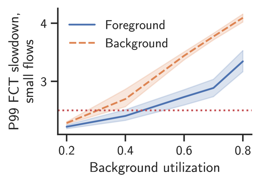
(a) CC + FIFO

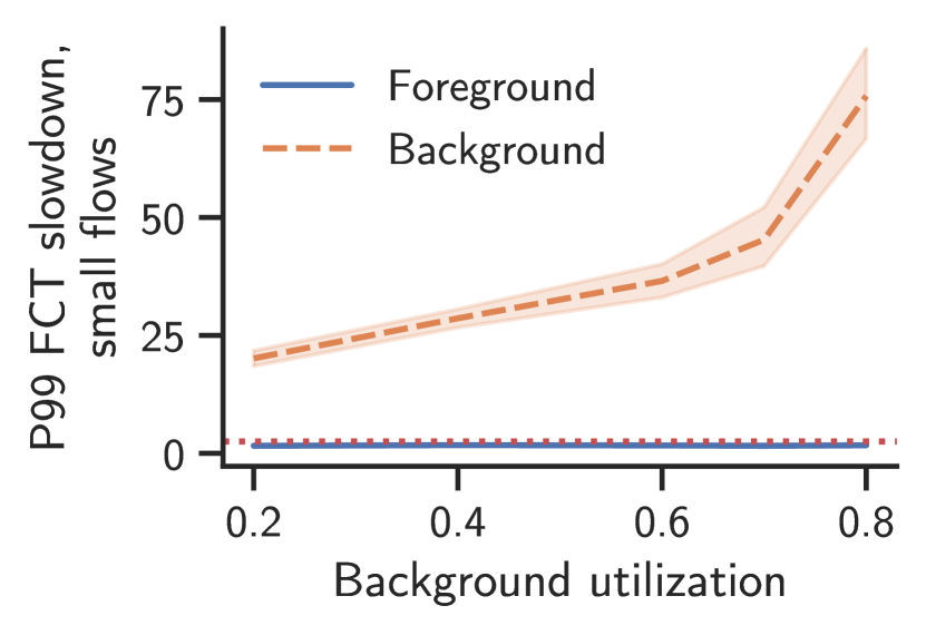
(b) CC + PQ

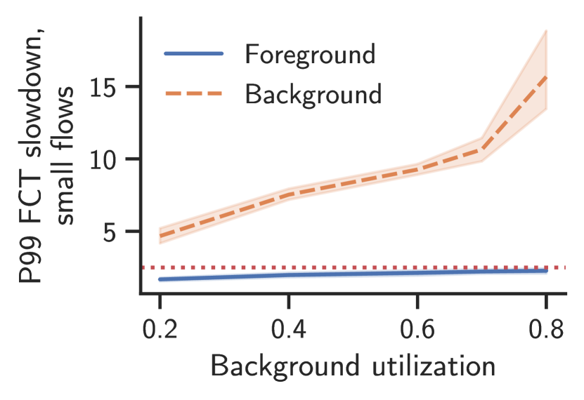
(c) CC + TC

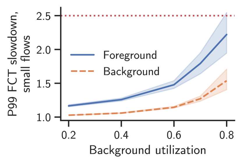
(d) FQ + TC

Figure 1. Tail (99%) message slowdown for the Homa W3 workload (homa, ). Foreground traffic is set to 10% of the link bandwidth, with variable background traffic. The dotted horizontal line shows a 2.5$\boldsymbol{\times}$ SLO, and the y-axis scale varies between graphs. Shaded regions represent the 95% confidence interval. We compare endpoint congestion control (CC) and a FIFO queue at the switch; CC and strict priority queueing (PQ); CC and per-traffic class (TC) scheduling weights at the switch, tuned to meet the foreground SLO with 80% background traffic; scheduling weights and per-traffic class fair queueing among queued flows. While priority scheduling can provide latency guarantees for foreground traffic, it leaves the tail latency of background traffic higher than necessary.

2.1. Limits of Priority Scheduling

To motivate the approach taken by swp, we develop a simple experiment to characterize the limitations of priority scheduling for providing feasible SLOs for non-priority traffic. Our evaluation of swp explores the parameter space more fully.

We start with a large number of servers connected by 100 Gbps links and a round-trip delay of 10 $\mathrm{\SIUnitSymbolMicro s}$. We focus on a single bottleneck, located near the destination, with traffic split between foreground (higher priority) and background (lower priority) traffic. Message sizes for both foreground and background traffic are drawn from the Homa W3 distribution (homa, ), taken as a sample of all messages in a Google data center. We assume the two traffic classes are independent of each other, but within each traffic class, flows have log-normal interarrival time distributions with a shape parameter $\sigma$ of two. Further, we assume HPCC congestion control with an initial window size of the bandwidth-delay product (hpcc, ).

For this experiment, we focus on 99% tail message slowdown for messages less than the bandwidth-delay product. In this workload, these account for the large majority of requests but less than half of the total bytes transferred. To test how well each configuration insulates foreground traffic from background traffic, we fix the foreground utilization at 10% and vary the background utilization from 20% to 80%. We choose a target slowdown of 2.5$\times$ for the SLO, that is, a tail latency for 125 KB messages of 50 $\mathrm{\SIUnitSymbolMicro s}$.

Fig. 1 compares the 99% tail message slowdowns for four configurations. First, we pair endpoint congestion control with a FIFO queue at the switch, shared between both foreground and background traffic (Fig. 1(a)). As expected, using a shared queue means that background traffic can interfere with foreground tail latency. At low load, both foreground and background traffic can achieve the target SLO. As background load increases, endpoint congestion control limits the effect of the background traffic on the foreground traffic, but at high enough loads, the unconstrained portion of the traffic (within the initial window) can impact foreground tail delay.

Note that the tail latency for foreground and background traffic differ. This is because the inter-arrival distribution is heavy-tailed and hence bursty within its own traffic class, but uncorrelated across traffic classes. Conditional on a small background message arriving at the switch, it is more likely that other background flows will already be queued at the switch; this is the definition of heavy-tailed behavior. Foreground traffic is more likely to encounter other foreground flows; however, the foreground load is lower so that occurs less often.

Next, we add strict priority scheduling at the switch, where foreground traffic always takes precedence over background traffic (Fig. 1(b)). This achieves the SLO for the foreground traffic regardless of the background traffic intensity, but only at the cost of much higher small message response time for background traffic. Note that the y-axis is rescaled to show the effect. Because the foreground traffic takes priority, if the background traffic arrives during a burst of foreground traffic, it will experience head-of-line blocking—no progress until the burst is cleared. This has a measurable effect on background tail latency, even though the foreground traffic uses only 10% of the link in aggregate.

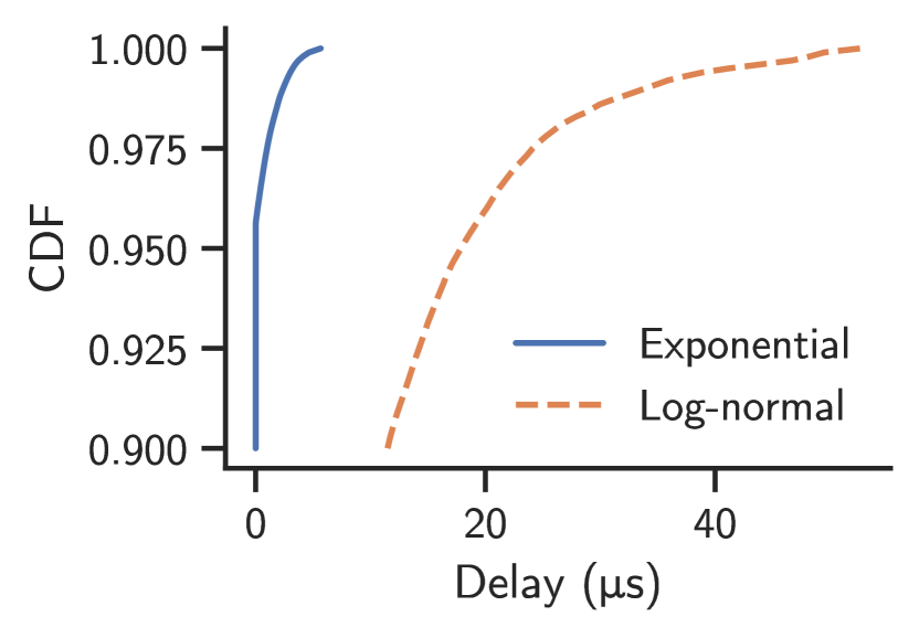
(a) Sensitivity to burstiness

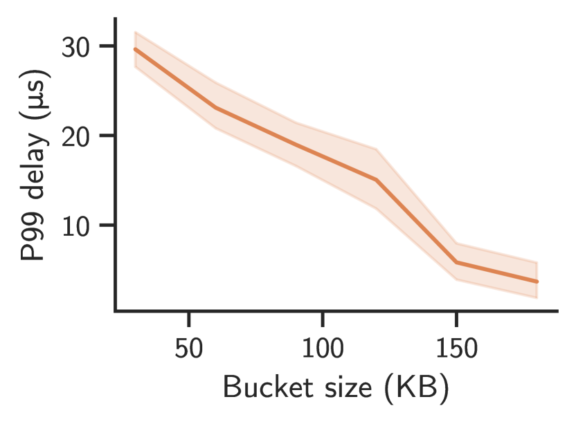
(b) Adjusting the bucket size

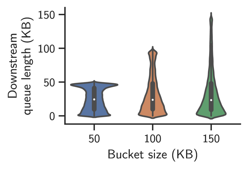
(c) Effect on downstream queues

Figure 2. When a workload is bursty, leaky bucket parameters must be tuned to preserve low tail delays at the host. However, this will in turn increase the tail of downstream queue lengths (as seen by an arriving packet).

Although not shown because of the y-axis rescaling, the foreground traffic achieves its SLO with considerable room to spare; in this scenario, prioritization is overly conservative, needlessly harming background tail latency.

The third graph in the figure (Fig. 1(c)) considers the impact of traffic class weights on SLOs. In this case, the switch has separate FIFO queues for each traffic class, and schedules among each queue according to its weight if both queues are occupied. When only one queue is occupied, that queue is scheduled. To our knowledge, there are no well-established guidelines for how to set traffic weights. Instead, data center operators act by trial and error—adjust weights to meet a specific SLO in a specific situation.

We model this by setting the foreground scheduling weight so that it meets its SLO tail latency target even for the highest level of background traffic (80% load), with a small margin of error. A single weight is able to insulate the foreground tail latency across the entire range of background traffic intensity, unlike CC+FIFO. Likewise, although the background traffic is unable to meet the target SLO, it experiences much better tail latency than with priority scheduling.

We could do even better for reducing background tail latency if we were to know in advance the average traffic intensity of the background traffic. At low background utilization, the traffic weights chosen above are needlessly strict. With less competing background traffic, we can afford to give the foreground traffic less weight—less headroom above its traffic demand—and still meet its SLOs. This is because most of the time the foreground traffic will arrive at the switch to find the background queue empty, improving its overall performance. This insight—that we should set weights given knowledge of the foreground and background traffic characteristics—lies at the core of the design of swp.

Finally, we consider the case of a programmable switch capable of implementing fair queueing (fq, ) through the use of calendar queues (cal-queues, ). We assume a hierarchical setting, where weights are used to choose among traffic classes when both have traffic present. Within each traffic class, separate calendar queues are used to implement fair queueing among flows with traffic queued within that class. Fair queueing allows better isolation between competing flows within the same traffic class, by eliminating head-of-line blocking. With a diversity of message sizes, with FIFO queueing a short message can be delayed behind packets of a longer flow. A fair queued system allows the short message to be scheduled earlier. Recall that we give the foreground traffic just enough weight to meet the SLO in the presence of background traffic at 80% load, with the remaining capacity given to the background traffic. With fair queueing, the foreground traffic requires so little weight to meet the SLO that the background traffic even outperforms it (Fig. 1(d)). In this case the SLO could be further tightened without incurring additional SLO violations. In $\S$3.3, we describe a more sophisticated and more general optimizer that can find weights to meet distinct SLOs for multiple traffic classes.

2.2. Deterministic Latency Bounds

Prior work in bounding network tail latency has used endpoint traffic shaping and worst case analysis to derive deterministic guarantees. These guarantees are, in a sense, stronger than what is provided by swp, in that they provide bounds on worst case behavior for queueing even at the tail, as long as packets are not corrupted in flight. On the other hand, particularly for large scale systems with bursty traffic, the bounds are substantially looser than what swp can provide.

For example, QJump (qjump, ) and Silo (silo, ) apply a send-side leaky bucket filter to constrain the worst case load in the network. Even if all nodes send a burst at exactly the same time, the leaky bucket will constrain the worst case queueing at the bottleneck to, roughly, the bucket size times the number of senders, provided that the switch is configured to give priority to these latency-sensitive packets. This follows from a classic result due to Parekh and Gallager: if 1) admission to a network is governed by leaky bucket, 2) the network uses fair queueing, and 3) the arrival rates are constrained to ensure stability, then the delay in the network can be bounded (parekh-gallager, ).

There are two important limitations that led us to use a probabilistic, rather than a deterministic, model. First, most datacenter network traffic is highly bursty (dc-traffic, ). When source bursts can exceed the bucket size, a leaky bucket mechanism will impose an additional queueing delay at the source, to prevent bursts from one node from compromising the SLO’s provided to another. Second, the latency bound scales in proportion to the product of the bucket size and the number of senders. As the number of possible senders increases, the allowable burst must decrease proportionately to keep the SLO constant. For example, for a small data center with 1000 servers connected by 100Gbps links and a bucket size of 10KB buffer per server, worst case latency is nearly a millisecond.

This places the network designer in a bind. Tighten the bucket size, and more delay is experienced at the source; loosen the bucket size, and the worst case network queueing goes up. We illustrate this with a simple experiment (Fig. 2). First, we consider the send side queue. In Fig. 2(a), we assume exponentially distributed message sizes, with an arrival rate 5% smaller than the leaky bucket rate $r$. We set the bucket size to yield reasonable send side tail latency with Poisson arrivals, and then consider what happens when we shift to moderately bursty arrivals (log-normal with a shape parameter of 1.5). Tail delays with the more realistic log-normal distribution are an order of magnitude higher than would be predicted under the analytically tractable model.

To compensate for burstier traffic, we can increase the bucket size, as shown in Fig. 2(b)—source queueing delay decreases. Unfortunately, this only trades queueing at the host for queueing further downstream. Fig. 2(c) shows the distributions of downstream queue lengths at different bucket sizes. For each distribution, the median, the quartiles, and a rotated kernel density estimation is drawn. We see that as the bucket size increases, so too does the tail of downstream queueing.

3. The swp Methodology

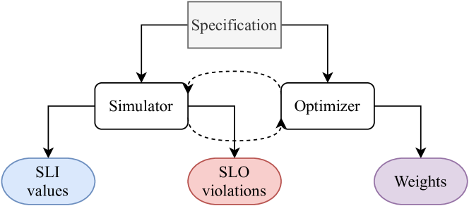
Figure 3. The swp workflow. Rectangular boxes indicate user inputs, rounded boxes indicate swp components, and ovals indicate outputs. Dashed lines show the optimization loop for finding weight allocations.

Our goal with swp is to build a tool to aid network operators with configuring their network switches to achieve tail latency SLOs for multiple classes of traffic. Specifically, swp

1. allows users to specify a network configuration, a set of traffic classes, and their SLOs,

2. automatically finds switch weights for meeting those SLOs (if possible), and

3. provides descriptive answers to what-if style questions about SLO behavior.

We begin with a brief overview of the swp workflow ($\S$3.1). Then, we show how to parameterize the network model and specify a traffic class’s SLOs ($\S$3.2). Lastly, we discuss how simulation outputs are used as input to a downstream optimizer, and we describe the one we use for automatically finding switch weights ($\S$3.3). The network simulator is described in detail in $\S$4.

3.1. Overview

Fig. 3 depicts swp’s workflow. For each traffic class, the user provides information about its flow sizes and interarrival times. These can be in the form of a trace, a measured cumulative probability distribution, or a generator function. Once the workloads have been characterized, the next steps are to specify each traffic class’s SLIs and SLOs ($\S$2) and describe the network used by the simulator in $\S$4. We use Dhall (dhall, ) as the configuration language because it allows for typed and modular configurations, and it can be converted to widely used formats like JSON and YAML. Specifications can be fed to either the simulator itself through the standard front end or to the weight optimizer. If the simulator is invoked directly through the front end, it will simply run the classes together according to the specification and return whether the SLOs are met or violated, and why. Alternatively, the optimizer will run the simulator many times in search of a suitable weight allocation.

3.2. Specification

⬇

1-- Top-level configuration

2{ network =

3 { link = T.Gbps 100

4 , rtt = T.Us 10

5 }

6, queue = Queue.FIFO

7, cc = ./dctcp.dhall

8, classes = [ ./foo.dhall, ./bar.dhall ]

9} : Config

10

11-- In ‘dctcp.dhall‘

12CC.Normal

13 { r_init = T.Gbps 100

14 , u_target = 1.0

15 , thresh = T.KB 100

16 , beta = 1.0

17 , eta = 5.5

18 }

19

20-- In ‘foo.dhall‘

21{ name = "Foo"

22, flowsizes = Workload.Cdf "websearch.txt"

23, interarrivals =

24 Workload.Lognormal

25 { mu = 11.3, sigma = 2.0 }

26, slis =

27 [ { name = "tail_slowdown"

28 , metric = Metric.Percentile 0.99

29 , attr = Attr.Slowdowns

30 -- ... (snip)

31 }

32 ]

33, slo = "tail_slowdown < 3.0"

34}

35-- ‘bar.dhall‘ is similar

Figure 4. An abridged specification with two traffic classes.

Fig. 4 shows an example specification for a network configuration, traffic classes, SLIs, and SLOs. First, we provide the link capacity and the round-trip time (lines 3–4), followed by the queueing discipline used at the bottleneck (line 6). The congestion control protocol is imported from dctcp.dhall (reproduced in lines 12–18). The meanings of the congestion control parameters are described in more detail in the next section. Likewise, the traffic classes Foo and Bar are imported from foo.dhall and bar.dhall, respectively.

We define a traffic class Foo on line 21. Foo’s message size distribution is given by the cumulative distribution in websearch.txt, as described in Homa (homa, ). For interarrival times, we approximate them using a log-normal distribution with mean $\mu$ equal to 11.3 and shape parameter $\sigma$ equal to 2.0. Together, the mean interarrival time and message size specify the average bandwidth required for this traffic class; the interarrival and message distribution, along with the congestion control protocol, control the burstiness of traffic at the bottleneck link.

To evaluate this traffic class’s performance, we select the 99th percentile slowdown as our SLI. We can also filter over flow size ranges in the SLI definition, but this is omitted from this example for brevity. The last step for Foo is to form an SLO by writing a logical predicate over the SLI (line 33). Here, we say that the P99 slowdown should be less than 3$\times$. We could also combine different SLIs with different thresholds, e.g., so that small messages can have a tighter bound than longer transfers.

The example includes a second traffic class Bar, defined in much the same way, but with independent choices for traffic size distribution, interarrival burstiness, SLIs, and SLOs.

Once the specification is written, the user can pass it to swp to ask it to make SLO predictions under simulation. The front end will:

1. Read and validate the specification.

2. Use the specification to build and run a simulation, which will terminate with a set of statistics.

3. Digest the statistics to populate the SLIs.

4. Predict whether or not each SLO will be met.

A key contribution is to make simulations fast enough that a large space of configurations and SLOs can be quickly explored. Upon completion, swp will produce a set of predictions. For each traffic class, it predicts a value for each SLI as well as a final prediction for the SLO. A slightly modified version of the specification can also be passed to the weight optimizer, which we describe next.

Algorithm 1 Weight optimization loop

1:baselines $\leftarrow$ FindBaselines(classes)

2:weights $\leftarrow$ Normalize(baselines) $\triangleright$ class to weight

3:success $\leftarrow$ False

4:while not timed out do

5:    losses $\leftarrow$ GetLosses(classes, weights) $\triangleright$ simulate

6:    losses $\leftarrow$ Sort(losses) $\triangleright$ (class, loss) pairs sorted by loss

7:    if all losses negative then

8:         success $\leftarrow$ True

9:         break     

10:    $\_$, $l_{\text{min}}$ $\leftarrow$ losses[0]

11:    if $l_{\text{min}}>0$ then

12:         break $\triangleright$ fail when min loss is positive     

13:    rev $\leftarrow$ reverse(losses)

14:    iterator $\leftarrow$ zip(losses, rev) $\triangleright$ iterate from both ends

15:    for ($k$, $l_{k}$), ($q$, $l_{q}$) in iterator do

16:         if $l_{k}\geq 0$ or $l_{q}\leq 0$ then

17:             break          

18:         $\Delta$ $\leftarrow$ $|l_{k}/2|\cdot\text{weights}[k]$ $\triangleright$ transfer amount

19:         weights[$k$] $\leftarrow$ weights[$k$] - $\Delta$

20:         weights[$q$] $\leftarrow$ weights[$q$] + $\Delta$     

21:return weights, success

3.3. A Weight Optimizer

The final component of swp is an optimizer that hooks into the simulator’s Rust API and searches for switch weights that can meet the SLOs of a set of traffic classes. To start, each traffic class defines a loss function that takes the simulation output and quantifies the distance between the observed SLI value and its target SLO threshold. For the purpose of tail latency SLOs, we assume the threshold is an upper bound, so if the value exceeds the threshold, then the class requires more capacity, but if the SLI is under the threshold, then the class potentially has extra slack that can be given to other classes. To compute loss, we simply use

(1) $$\text{loss}=-\frac{\text{SLO threshold}-\text{SLI value}}{\text{SLO threshold}}.$$

Here, a negative loss indicates the SLO is met, and a positive loss indicates the SLO is missed.

To find a starting point for the search process, we define a baseline weight allocation for each class: the minimum normalized switch weight a class requires to meet its SLO assuming worst case behavior by all other competing traffic classes—that is, that all other traffic classes always have a packet queued at the bottleneck switch. We use a binary search for this; each class’s baselines are found in parallel.

Once the baselines are found, we normalize them such that they sum to one, and then we enter the optimization loop. At each step of the loop, we first compute the losses by running the classes together in simulation and then sorting their losses in ascending order. Then in an inner loop we iterate through the losses from both ends simultaneously, with the minimum loss class paired with the maximum loss class, and so on. If class $k$ is paired with class $q$, and if $k$ met its SLO while $q$ did not, then we simply transfer weight from $k$ to $q$ in proportion to $k$’s loss. The optimization succeeds when all losses are negative, and it fails when either 1) no loss is negative or 2) the optimization loop times out. Pseudocode for the optimization loop is shown in Alg. 1.

4. A Network Model

Because it runs as the inner loop of swp, our network model is designed to be as simple as possible while still making accurate predictions about the aggregate tail SLO behavior seen in a network. Like any model, it will necessarily diverge from reality. Our goal, however, is not to represent the network stack with full fidelity but to isolate and represent the aspects are most significant for whether tail SLOs are met by a particular configuration.

The need for something that is simple and fast is motivated in part by our experience with ns-3 (ns-3, )—a thorough and widely-used network simulator—whose attention to detail lends it high fidelity, but whose explicit modeling of protocol mechanisms prevents rapid answers to what-if questions. ns-3 simulates every packet arrival and departure at every link, queue, and host, along with host timeouts and the full host network protocol stack, with multiple events to send a packet through transport, network, and link layers. Particularly for establishing confidence intervals in tail behavior with bursty workloads, this level of detail can make simulations take hours rather than minutes. Using ns-3 would also place a limit on how quickly swp could react to measured changes in workload.

We believe that a model of the network can be useful even if it ignores most of the above details, especially if it is only used to reason about aggregate statistical behavior. The central challenge, however, is defining one that adequately balances simplicity against fidelity. One of our contributions is a functional, rather than an operational, model of the network to try to better strike this balance.

4.1. Overview

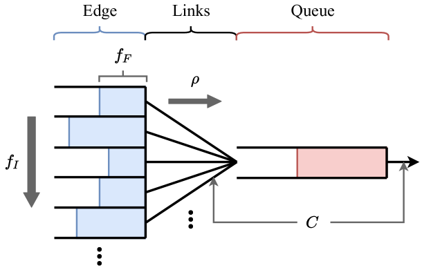
Figure 5. A simple network model with a single bottleneck where all links have capacity $\boldsymbol{C}$. Flows arrive according to some flow size and interarrival time distribution, and each flow $\boldsymbol{i}$ sends at some rate $\boldsymbol{\rho_{i}\leq C}$.

Fig. 5 depicts the network model. All links have capacity $C$, and there is a single bottleneck with an infinite queue, following some queueing discipline. Flows are generated at the edge with flow sizes and interarrival times drawn from distributions $f_{F}$ and $f_{I}$. Upon arrival, each flow $i$ begins sending data at some rate $\rho_{i}$ governed by a model of congestion control (described in the next section). The delay between sources at the edge and the bottleneck is $\tau$ (giving a round-trip time of $2\tau$).

Restricting the model to include only a single bottleneck queue in this manner is a simplification, but meeting SLOs in even this simple case is nontrivial. Moreover, where congestion is caused by incast or fan-in, there is only one bottleneck, and Google has previously reported that last hop congestion is the most common in datacenters (jupiter, ). In Section $\S$5.1, we compare predictions made by simulating against this model to those made by ns-3 on a single bottleneck link.

4.2. Congestion Control

While usually complex, congestion control algorithms often have a functional description that can be succinctly summarized. For example, a particular algorithm will react to congestion signals, choose a balance between utilization and queueing, and converge to a target bandwidth allocation after some number of steps. Our goal is to design a model that captures these characteristics. Throughout, we use the notation $x^{+}$ to mean $\max(0,x)$. First, for any given flow, its ideal sending rate at time $t$ is denoted $R(t)$, and it is given by

(2) $$R(t)=\begin{cases}r_{\text{init}}&t\leq 2\tau\\ r(t)^{+}&\text{otherwise}\\ \end{cases},$$

where $r(t)$ is an update rule which will be described shortly. Recall that $\tau$ is the one-way delay between the sources and the bottleneck. Upon arrival, a new flow begins sending immediately at some initial rate $r_{\text{init}}$, and it will continue sending at this rate until it receives congestion control feedback at time $2\tau$. Many modern datacenter protocols, such as DCQCN (dcqcn, ) and HPCC (hpcc, ), set $r_{\text{init}}$ to the line rate $C$. For protocols with a smaller $r_{\text{init}}$ value, we assume the initial window is paced (tcppacing, ) rather than ack clocked. We model the feedback delay explicitly because it has important implications on the number of uncontrolled bytes in the network. As link speeds increase and flow size distributions skew smaller, a greater fraction of traffic is transmitted in an uncontrolled manner (bfc, ; aeolus, ).

Update rule.

The update rule $r(t)$ defines the core of the control loop, and it applies to a flow as soon as the flow first receives feedback. At this time, we say the flow is controlled. Likewise if a flow has begun sending but has not yet received feedback, we say it is uncontrolled. Given this terminology, a high-level and idealized description of the update rule is

$$\text{rate}=\frac{\text{total capacity}-\text{uncontrolled rate}-\text{queue drain}}{\#\text{ of controlled flows}},$$

where “uncontrolled rate” refers to the total sending rate across all uncontrolled flows. This rule follows our intuition that the rate at which a controlled flow should send at any given time depends on how much residual capacity there is at the bottleneck—and that, in turn, depends on 1) how much uncontrolled traffic there is and 2) how much queueing has accumulated at the switch. For simplicity we do not model differences in fairness, so the residual capacity is simply divided evenly among all controlled flows.

We build on this idealized version by introducing delays in signal propagation as well as parameters for approximating different congestion control algorithms. We begin by defining the uncontrolled rate more precisely. Let $i$ be an arbitrary flow, $S_{i}$ be its initial size, and $t_{\text{a},i}$ be its arrival time. The uncontrolled rate contributed by this flow $i$ at time $t$, called $r_{\text{u},i}(t)$, is given by

(3) $$r_{\text{u},i}(t)=\begin{cases}\dfrac{\min(r_{\text{init}}\cdot 2\tau,S_{i})}{2\tau}&0\leq t-t_{\text{a},i}\leq 2\tau\\ 0&\text{otherwise}\\ \end{cases}.$$

In other words, each flow will contribute up to $r_{\text{init}}\cdot 2\tau$ uncontrolled bytes upon arrival, paced out over $2\tau$ time. The total uncontrolled rate at time $t$ is then just the sum over the individual flows,

(4) $$r_{\text{u}}(t)=\sum_{i}r_{\text{u},i}(t).$$

Next, the number of controlled flows at time $t$ is simply the number of flows that have already sent $r_{\text{init}}\cdot 2\tau$ bytes and are still sending at time $t$:

(5) $$N(t)=\big{|}\{i\mid t-t_{\text{a}}>2\tau\text{ and }i\text{ has unsent bytes}\}\big{|}.$$

And finally, let $Q(t)$ be the number of bytes queued at the bottleneck at time $t$.

We are now ready to state the update rule $r(t)$. Recalling that $C$ is the total link capacity, the update rule for each controlled flow is

(6) $$r(t)=\frac{U\cdot C-\beta\cdot r_{\text{u}}(t-2\tau)-\dfrac{(Q(t-\tau)-T)^{+}}{2\tau}}{N(t-2\tau)},$$

where $U$, $\beta$, and $T$ are parameters to the congestion control model. Different settings will approximate different congestion control algorithms.

The parameter $U$ is the target utilization, and $\beta$ is always zero or one, controlling whether or not the model reacts to the uncontrolled rate. These parameters are meant to model an algorithm like HPCC (hpcc, ), which 1) tries to keep near-zero queues by intentionally underutilizing links, and 2) can detect congestion without waiting for queueing to occur. On the other hand, algorithms like DCTCP (dctcp, ), DCQCN (dcqcn, ), and TIMELY (timely, ) can only detect congestion after a queue builds up. In this case, $\beta$ would be set to zero, and the threshold at which the model reacts to queueing is controlled by $T$.

We also note the time delays on $r_{\text{u}}$, $Q$, and $N$. These reflect our intuition about which signals are collected at the sources ($t-2\tau$), and which signals are collected at the switch ($t-\tau$). For example, a new flow that arrives cannot have its uncontrolled rate affect the rates assigned to other flows until $2\tau$ after its arrival. However, since queueing is measured at the bottleneck, the buildup of a queue can be indicated to sources after $\tau$ time.

Convergence speed.

Recall that $R(t)$ from (2) is the ideal sending rate of a flow at time $t$, as determined by the parameters and the model. The actual rate assigned to flows $\rho(t)$ will converge to $R(t)$ on a certain timescale dictated by the convergence speed of the congestion control algorithm. The convergence timescale is controlled by a smoothing parameter $\eta$:

(7) $$\frac{d\rho}{dt}=\frac{R(t)-\rho(t)}{\eta\tau}.$$

This differential equation is the continuous-time equivalent of applying an exponentially weighted moving average (first-order low pass filter) to $R(t)$ to derive $\rho(t)$. Higher values of $\eta$ will result in slower convergence. A full listing of the model’s congestion control parameters are given in Table 1.

Model parameter	Description
$r_{\text{init}}$	Initial send rate
$U$	Target utilization
$T$	Queue threshold
$\beta$	Uncontrolled traffic reaction
$\eta$	Convergence smoothing

Table 1. swp’s congestion control parameters.

Multiple traffic classes.

The above model assumes there is only one class of traffic, but algorithms like DCTCP can be adapted to the case where there are multiple traffic classes, and each class is associated with a fixed scheduling weight at the switch. Here, we describe how to generalize the model to cover this scenario. To state our goal concretely, suppose there are $n$ classes, and suppose $k$ is an arbitrary class—with weight $w_{k}$—that is continuously backlogged on some time interval. Then in the congestion control model, we want the capacity $C_{k}$ that is available to class $k$ to be such that

(8) $$C_{k}\geq\frac{w_{k}}{\sum_{l=1}^{n}w_{l}}C$$

on that time interval. Moreover, if a class is not using the link, its capacity should be divided among all active classes in proportion to their weights.

First, we restrict congestion signals $r_{\text{u}}$, $Q$, and $N$ to only include information about a particular class $k$, yielding $r_{\text{u},k}$, $Q_{k}$, and $N_{k}$. For example, $r_{\text{u},k}$ would be the total rate of uncontrolled traffic due to class $k$. Now we define the model’s notion of an active class. We say a class $k$ is active at time $t$ when at least one of two conditions holds:

1. $Q_{k}(t)>0$, or

2. $k$ has a packet on the bottleneck wire at time $t$.

For convenience, we define a predicate $\text{active}_{k}(t)$ which is true whenever the above criterion is met for class $k$. We will also define a function $W$ which maps a set of class indices $K$ to the sum of the class’ weights,

(9) $$W(K)=\sum_{k\in K}w_{k}.$$

With these definitions, we can write the bottleneck capacity available to class $k$ at time $t$ as

(10) $$C_{k}(t)=\frac{w_{k}}{W(\{l\mid\text{active}_{l}(t)\}\cup\{k\})}C.$$

Unlike in the original definition of $r(t)$ in (6), we now have a link capacity that is time varying. Substituting this as well as the class-specific signals from above, we can write the update rule for class $k$ as

(11) $$r_{k}(t)=\frac{U\cdot C_{k}(t-\tau)-\beta\cdot r_{\text{u},k}(t-2\tau)-\dfrac{(Q_{k}(t-\tau)-T)^{+}}{2\tau}}{N_{k}(t-2\tau)}.$$

Aside from the update rule, everything in the multi-class case works in the same way as before.

4.3. Queueing Discipline

We consider several standard queueing disciplines: first-in first-out (FIFO), priority queueing (PQ), round robin (RR), deficit round robin (DRR), as well as common hierarchical and weighted variants. Some of these policies had long been considered impractical to implement on switches, but recent work has shown how the mechanisms on newer programmable switches can be used to approximate policies like weighted fair queueing (cal-queues, ). We include a variety of policies in our model to observe their impact on SLOs.

5. Evaluation

5.1. Evaluating the Network Model

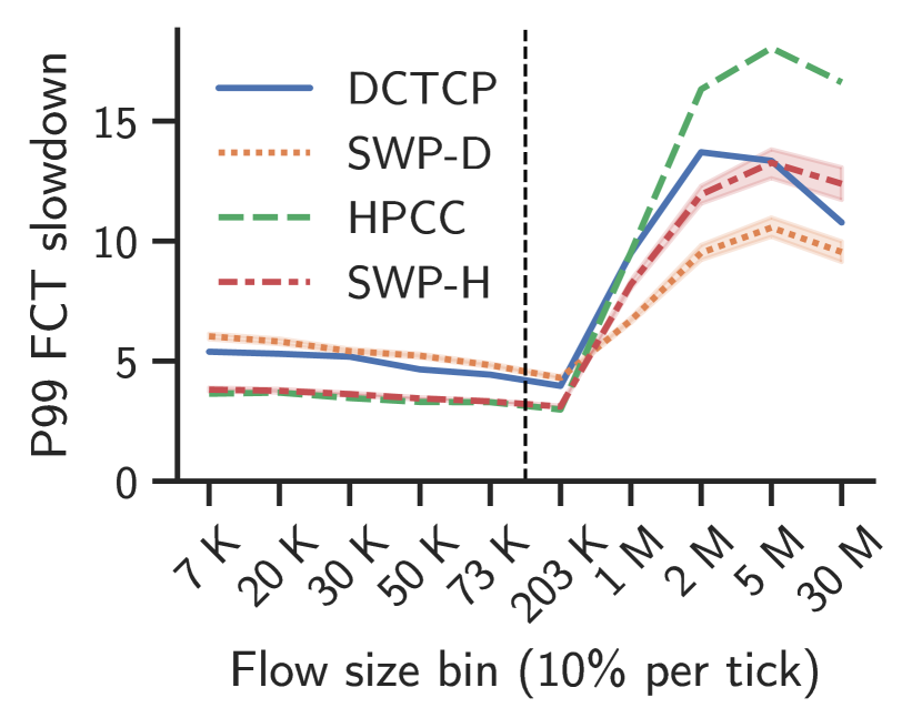
(a) WebSearch, 30% utilization

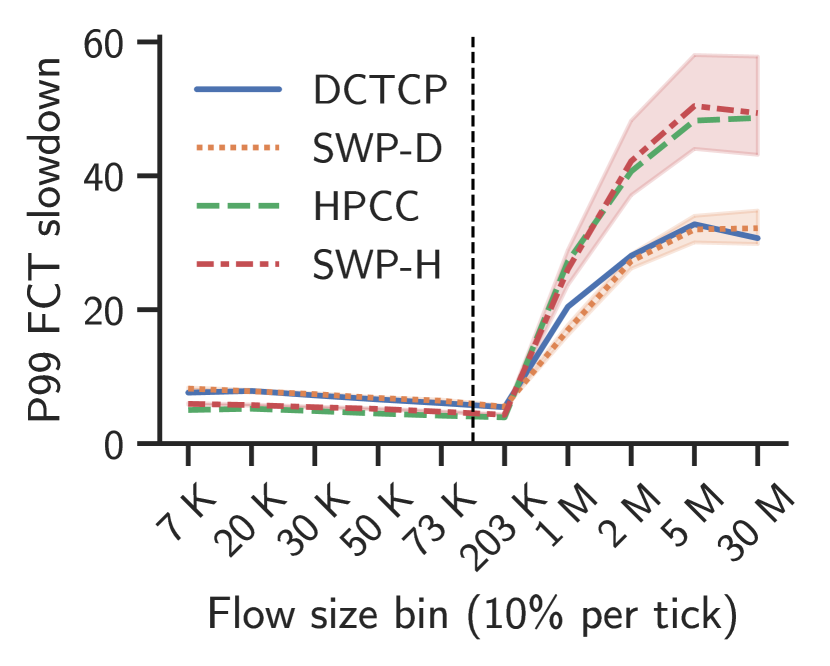
(b) WebSearch, 60% utilization

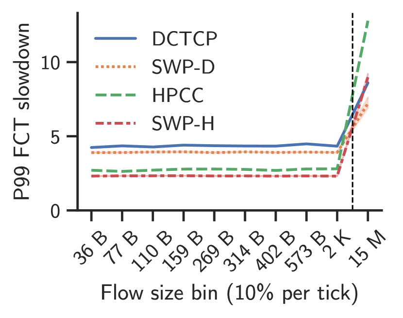
(c) Google, 30% utilization

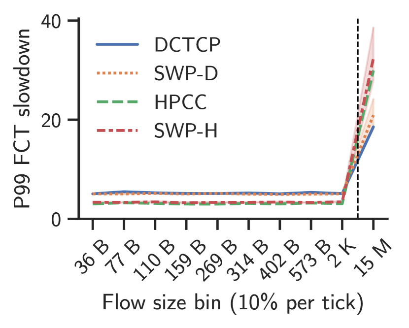
(d) Google, 60% utilization

Figure 6. When there is a single bottleneck, swp’s network model is effective at predicting the P99 slowdown of short flows under DCTCP and HPCC. Here, SWP-D and SWP-H are tuned to match the behavior of DCTCP and HPCC, respectively, by setting the congestion control parameters (Table 1) to those shown in Table 2. Once the parameters are set, they are unchanged across load levels and flow size distributions. Binning is done according to flow size. In this experiment, there are ten equally-sized bins, and each tick on the horizontal axis is labeled with the largest flow size in the corresponding bin. The dashed vertical line approximately indicates one BDP.

Parameter	SWP-D	SWP-H
$r_{\text{init}}$	100 Gbps	100 Gbps
$\boldsymbol{U}$	100%	90%
$\boldsymbol{T}$	100 KB	0 KB
$\boldsymbol{\beta}$	0.0	1.0
$\boldsymbol{\eta}$	5.5	5.0

Table 2. The congestion control parameters used for SWP-D and SWP-H in Fig. 6. Bolded rows indicate where parameters differ between the two configurations.

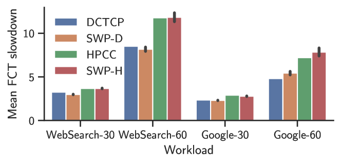
Figure 7. For flows larger than a megabyte, SWP-D and SWP-H can approximate the mean slowdown given by DCTCP and HPCC. Labels on the horizontal axis give the flow size distribution and the utilization.

Workload	ns-3	swp	Slowdown
WebSearch-30	113.22	1.68	67.39$\boldsymbol{\times}$
WebSearch-60	124.69	2.35	53.06$\boldsymbol{\times}$
Google-30	54.77	0.67	81.75$\boldsymbol{\times}$
Google-60	55.95	0.80	69.94$\boldsymbol{\times}$

Table 3. swp’s simplified model allows a simulator to simulate 50,000 flows over 50$\boldsymbol{\times}$ faster than ns-3 in a comparable scenario. Here, ns-3 is running DCTCP and swp is running SWP-D. Running times are shown in minutes.

Before using swp to predict SLOs, we first evaluate our network model by comparing its predictions to the output of ns-3 simulating a single bottleneck link. For a higher degree of confidence, we try different flow size distributions at different load levels using both DCTCP and HPCC, and we analyze tail latencies across fine-grained flow size bins. The goal of the model is not to report accurate predictions for per-flow statistics, but rather to capture information about aggregate statistics like the averages and tails of flow completion times (FCTs). This is what allows us to distill complex behavior into a simple model and achieve quicker answers to the questions we are trying to ask.

Specifically, we evaluate the model along three axes:

1. How well does the model predict the tail FCT slowdown of short flows?

2. How well does the model predict the average FCT slowdown of long flows?

3. How much faster is the model when compared to ns-3?

For short flows, we believe the model should accurately predict tail slowdowns, since those will depend largely on the aggregate behavior of the congestion control model defined in $\S$4.2. However, since we explicitly do not model differences in fairness among long flows, we do not always expect accurate tail predictions for them. For these flows, we instead evaluate the model’s ability to predict accurate average slowdowns. This reflects common practice, since short messages often require low, predictable latency while long ones should achieve acceptable throughput.

In these experiments, we use a 100 Gbps bottleneck link and a 10 $\mathrm{\SIUnitSymbolMicro s}$ round trip time (RTT). We configure ns-3 with multiple sources sending to the same destination through a bottleneck, similarly to the model shown in Fig. 5. We use two publicly available flow size distributions: one is a web search application (dctcp, ), and the other is an aggregated workload from a Google datacenter (homa, ). The workloads are run with a bursty log-normal interarrival time distribution (shape parameter $\sigma=2$) at two different load levels, 30% and 60%. We also run them with both DCTCP and HPCC.

Fig. 6 shows the tail FCT slowdown predictions produced by the model across these configurations and across equally-sized flow size bins. For short flows, the model is able to accurately predict the slowdowns at the 99th percentile, and at 60% utilization it can even reasonably predict the tail slowdown of long flows. At low utilization, the tail predictions for long flows are less accurate because 1) the model does not model short-term unfairness for long flows and 2) at low utilization events have higher variance, and this increases the tail variance of long flows. The average FCT slowdown for long flows, however, remains accurate across load levels. This is shown in Fig. 7. Lastly, the model arrives at these predictions up to 80$\times$ faster than does ns-3. Table 3 shows the running time of ns-3 running DCTCP compared against swp’s model, with measurements taken on an Intel Xeon E5-2680 CPU. The swp simulator simulates 50,000 flows up to 81$\times$ faster than does ns-3. Running times for HPCC and its corresponding swp model are similar.

5.2. Evaluating Network Configurations

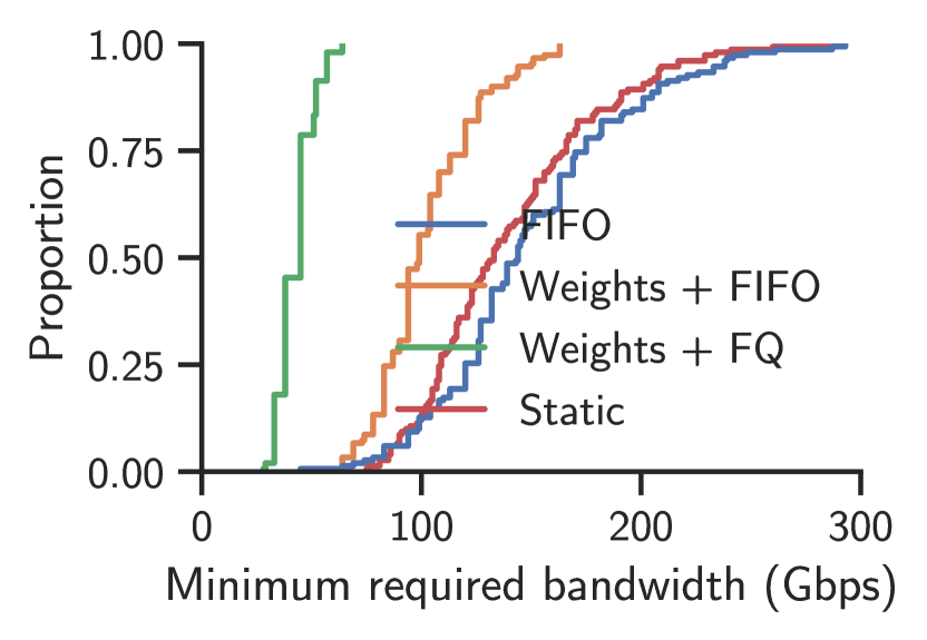
(a) All configurations

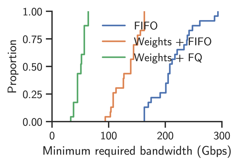
(b) Configurations with at least one tight SLO (threshold $<$ 4) on a bursty class ($\sigma>$ 1.7)

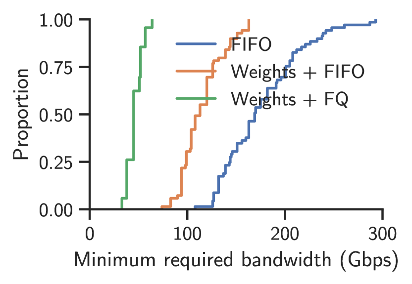
(c) Configurations with at least one tight SLO (threshold $<$ 4)

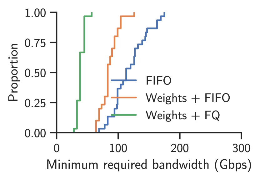
(d) Configurations with no tight SLOs and lower burstiness (all thresholds $\geq$ 4 and all $\boldsymbol{\sigma\leq 1.7}$)

Figure 8. swp finds weights that can meet a set of SLOs using significantly less bandwidth than would be required with pure FIFO queueing. The advantage of weights over FIFO is yet more pronounced with tighter SLOs and higher application burstiness.

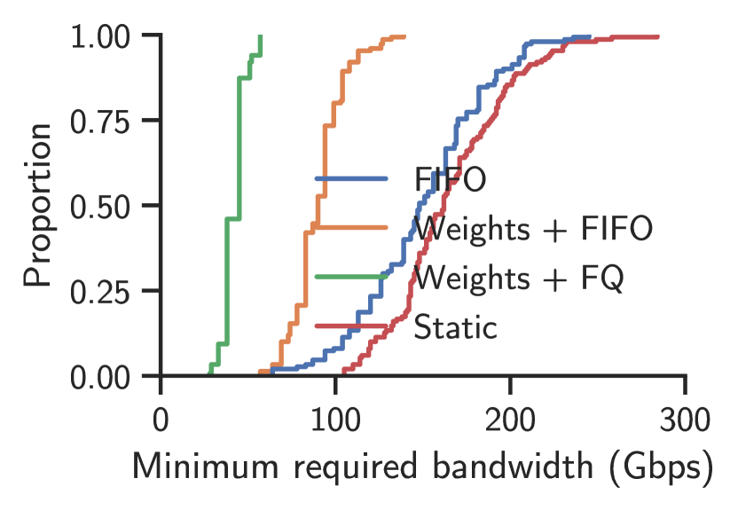
(a) All configurations

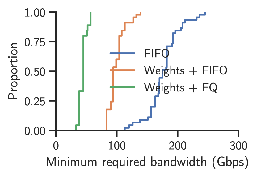
(b) Configurations with at least one tight SLO (threshold $<$ 4) on a bursty class ($\sigma>$ 1.7)

Figure 9. When we choose five random traffic classes instead of three, the benefit of optimizing weights increases. Moreover, statically provisioning each class for the worst case becomes costlier than using pure FIFO.

Parameter	Sample space
Flow sizes	Google, Facebook, Alibaba
Burstiness ($\sigma$)	[1.0, 2.0]
Mean rate (3-class)	[5 Gbps, 10 Gbps]
Mean rate (5-class)	[3 Gbps, 6 Gbps]
SLO threshold	[3.0, 8.0]

Table 4. The sample space for the random configurations used in Fig. 8 and Fig. 9. The Google flow size distribution is the same as the one in $\S$5.1, and the Facebook and Alibaba distributions are taken from the public repository of HPCC (hpcc-repo, ). Burstiness is the shape parameter $\boldsymbol{\sigma}$ for the log-normal interarrival time distribution.

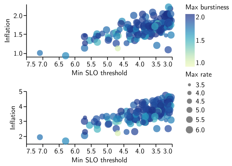
Figure 10. Minimum bandwidth inflation of FIFO over Weights+FIFO (top) and Weights+FQ (bottom), where inflation is defined as the quotient of the minimum bandwidth requirements. Each circle is a configuration with five traffic classes. For each one, we track the minimum SLO threshold, the maximum burstiness, and the maximum mean rate. Here we see that the tighter the SLO threshold, the higher the inflation on average.

We next use the optimizer described in $\S$3.3 to evaluate swp’s ability to identify switch configurations that meet target SLOs. Whether a particular configuration can be satisfied by swp, a FIFO queue, or both is a coarse-grained metric. Instead, we generate a randomly generated set of scenarios, and consider the minimum total bandwidth at the bottleneck that is sufficient to meet the combined SLO for that configuration. Lower required bandwidth for the same scenario is better—it implies that the same SLOs can be met with higher link utilization on a fixed bandwidth link. We do not consider priority scheduling in this experiment as that would require extremely high link capacities to meet the target SLOs, requiring very long runtimes to reach convergence at the tail.

We compare shared FIFO, per-class scheduling weights chosen by swp with FIFO within each class, and the same with fair queueing within each class. We consider scenarios with three simultaneous traffic classes, and to cover a wide range of cases, we sample traffic class characteristics randomly. For each class, we uniformly select at random a flow size distribution from three measured datacenter workloads, a burstiness (log-normal $\sigma$) between 1 - 2, a mean sending rate between 5-10 Gbps, and an SLO threshold for 99% tail latency slowdown between 3 - 8$\times$. We divide transfers into those that are smaller than the bandwidth-delay product for this network (125KB) and those that are larger. The tail latency slowdown is enforced against both sets independently, but with twice the slowdown threshold for larger flows. This is to allow solutions that favor small flows, without unduly starving medium-sized flows. Table 4 summarizes the sample space from which the random values are drawn. We use a 10 $\mathrm{\SIUnitSymbolMicro s}$ round trip time, and where congestion control applies, we use the model of DCTCP.

For each of 150 randomly chosen scenarios, we use swp to search for the minimum link capacity required to simultaneously meet all three SLOs for both small and large flows, separately for per-class FIFO and an idealized version of per-class fair queueing. We also use binary search to identify the minimum link capacity needed to meet the SLOs with a shared FIFO queue at the bottleneck.

Fig. 8(a) shows the cumulative distribution function for the minimum link capacity under different strategies and traffic scenarios. Averaged across all configurations, using FIFO alone requires on average 44% more link bandwidth than if swp is used to optimize per-class FIFO weights, and an average of 247% more bandwidth than with swp with optimized hierarchical weighted fair queueing.

If we restrict the configurations to those with at least one bursty class ($\sigma>1.7$) with a tight SLO (threshold $<$ 4), the average gap between swp and FIFO widens to 62% (Fig. 8(b)). Fig. 8(c) shows the results for configurations with SLO $<$ 4, but no restriction on burstiness, while Fig. 8(d) shows the results with all SLOs $\geq$ 4 and burstiness $\leq$ 1.7. The greatest advantage for swp comes on more challenging scenarios.

We can also ask: how important is the swp optimizer described in Algorithm 1 to the benefits of our approach? To study this, we consider a static version of swp, where we compute the bandwidth needed for each traffic class to meet its SLOs independently, assuming no knowledge of the behavior of the other traffic classes. We then run this on the same scenarios as we considered above. The result is plotted on the same graph in Fig. 8(a), labeled as static. The benefits of swp relative to FIFO roughly disappear—that is, the advantage of per-class SLOs comes from being able to take advantage of the cumulative slack across traffic classes.

Next, we consider configurations with five random traffic classes instead of three, where we keep aggregate load the same by adjusting per-class mean rates to be from 3 to 6 Gbps. The result is shown in Fig. 9. With more traffic classes, there is greater diversity of requirements, presenting more opportunities for optimization. In this setting, using FIFO queueing alone now requires 65% more link bandwidth than using optimized FIFO weights (Fig. 9(a)), and in the challenging scenario of a tight SLO on a bursty class, that number increases to 79% (Fig. 9(b)). Statically provisioning bandwidth for the worst case is also now more costly than pure FIFO queueing.

Finally, the inflation factor of a configuration is the ratio between the bandwidth required to meet SLOs with FIFO, divided by (respectively) that required by swp weights with per-class FIFO and swp with per-class fair queueing. Fig. 10 provides a scatter plot of inflation factors for all 150 five-class configurations, with each configuration indexed by the value of the tightest SLO, the greatest burstiness, and the greatest mean rate across the five traffic classes. In general, configurations with tighter SLOs show greater benefit for carefully optimized per-class traffic weights.

6. Related Work

Achieving quality of service in packet switched networks is a long-standing and rich research area. Quality of service is easiest to achieve when we can assume that switches or routers can keep per-flow state, such as Autonet-2 (an2, ), Intserv (intserv, ), and RSVP (rsvp, ). Parekh and Gallager showed that packet latency bounds could be provided given fair queueing in the network (fq, ; parekh-gallager, ). Others have shown it is possible to emulate fair queueing without per-flow state at every router (csfq, ). However, because of the difficulty of implementing these approaches at high speeds, most work in the Internet gravitated to the use of priorities (diffserv, ) to deliver quality of service. The underlying assumption was that only a small amount of near constant-bit rate traffic would need prioritization. By contrast, our work focuses on providing quality of service for datacenter traffic, where most or almost all network requests have timeliness constraints and the traffic demand is inherently bursty.

Per-packet latency guarantees. The closest to our work are QJump (qjump, ) and Silo (silo, ) as they both target providing quality of service guarantees in the datacenter. Both use a leaky bucket at sources to ensure senders do not exceed some average rate and burstiness allowance. Then, QJump uses switch priorities to bound the network packet delays for latency sensitive applications. SILO on the other hand uses network calculus to develop a VM placement algorithm that can ensure network queueing delays do not exceed some bound. Like earlier work, these approaches target individual packet delays, rather than application-level metrics, and traffic shaping can impose significant delays at the source particularly for bursty traffic. Moreover, for large scale datacenter networks, tight worst-case bounds can only be provided for a small fraction of the traffic. Our goal with swp is to provide quality of service for arbitrary size messages for most or all of the network traffic, using probabilistic rather than deterministic guarantees.

Scheduling flows for low latency. A number of systems, such as D³ (d3, ), D²TCP (d2tcp, ), and PDQ (pdq, ) use deadlines to schedule flows for low latency. pFabric (pfabric, ) uses shortest remaining time first to reduce average latency for short flows. A significant limitation with these approaches is that they require applications to provide the size of each flow, before it starts, to be able to assign it a deadline or scheduling priority. Many applications in wide use lack this information, and in fact the UNIX socket API does not allow applications to specify it even if known. In addition, these schemes require switch hardware modifications. swp helps operators achieve SLOs without new switch hardware or changing applications, provided aggregate information is available about the distribution of flow sizes and burstiness.

Homa (homa, ) is a transport protocol that uses switch priorities and receiver-driven use of priority queues to achieve low tail latency for short messages with existing hardware. Like these other approaches, however, Homa assumes the size of the flow is available. It also lacks a mechanism for predicting what tail latency guarantees it can provide, nor does it provide an algorithm for balancing SLOs across traffic classes or flow sizes.

7. Conclusion

In this paper, we have built and evaluated swp, a new tool for quickly identifying network switch configurations to achieve tight tail latency bounds for bursty datacenter traffic patterns. Given measured data about the distribution of message sizes and message interarrival times, swp finds traffic-class based switch scheduling weights to accomplish class-specific operator-defined service level objectives (SLOs). A key innovation is a 50-80$\times$ faster network simulation engine that elides detail but produces accurate estimates of tail behavior through a bottleneck link for two popular data center congestion control protocols, DCTCP and HPCC, for a variety of switch scheduling algorithms. We use swp on randomly chosen scenarios to show that swp can identify switch configurations that meet target SLOs at much lower bandwidth than FIFO.

This work does not raise any ethical issues.

References

- [1] High-Precision-Congestion-Control. https://github.com/alibaba-edu/High-Precision-Congestion-Control, 2019. [HPCC repository; commit 14cf7a3].
- [2] ns-3 Network Simulator. https://www.nsnam.org, 2020. [accessed Aug. 2020].
- [3] The Dhall configuration language. https://dhall-lang.org, 2021. [accessed Jan. 2021].
- [4] A. Aggarwal, S. Savage, and T. E. Anderson. Understanding the performance of TCP pacing. In Proceedings IEEE INFOCOM 2000, pages 1157–1165, 2000.
- [5] A. G. Alcoz, A. Dietmüller, and L. Vanbever. SP-PIFO: Approximating Push-In First-Out Behaviors using Strict-Priority Queues . In 17th USENIX Symposium on Networked Systems Design and Implementation (NSDI 20), pages 59–76, Feb. 2020.
- [6] M. Alizadeh, A. Greenberg, D. A. Maltz, J. Padhye, P. Patel, B. Prabhakar, S. Sengupta, and M. Sridharan. Data Center TCP (DCTCP). In Proceedings of the ACM SIGCOMM 2010 Conference, pages 63–74, 2010.
- [7] M. Alizadeh, S. Yang, M. Sharif, S. Katti, N. McKeown, B. Prabhakar, and S. Shenker. Pfabric: Minimal near-optimal datacenter transport. In Proceedings of the ACM SIGCOMM 2013 Conference on SIGCOMM, SIGCOMM ’13, page 435–446, New York, NY, USA, 2013. Association for Computing Machinery.
- [8] T. E. Anderson, S. S. Owicki, J. B. Saxe, and C. P. Thacker. High speed switch scheduling for local area networks. ACM Trans. Comput. Syst., 11(4):319–352, 1993.
- [9] L. Barroso, M. Marty, D. Patterson, and P. Ranganathan. Attack of the Killer Microseconds. Commun. ACM, 60(4):48–54, Mar. 2017.
- [10] T. Benson, A. Anand, A. Akella, and M. Zhang. Understanding data center traffic characteristics. SIGCOMM Comput. Commun. Rev., 40(1):92–99, Jan. 2010.
- [11] S. Blake, D. Black, M. Carlson, E. Davies, Z. Wang, and W. Weiss. RFC 2475: An Architecture for Differentiated Services, 1994.
- [12] R. Braden, D. Clark, and S. Shenker. RFC 1633: Integrated Services in the Internet Architecture: an Overview, 1994.
- [13] Broadcom. StrataXGS. https://www.broadcom.com/products/ethernet-connectivity/switching/strataxgs.
- [14] A. Demers, S. Keshav, and S. Shenker. Analysis and simulation of a fair queueing algorithm. SIGCOMM Comput. Commun. Rev., 19(4):1–12, Aug. 1989.
- [15] P. Goyal, P. Shah, K. Zhao, N. K. Sharma, M. Alizadeh, and T. E. Anderson. Backpressure Flow Control. arxiv:1909.09923, 2019.
- [16] M. P. Grosvenor, M. Schwarzkopf, I. Gog, R. N. M. Watson, A. W. Moore, S. Hand, and J. Crowcroft. Queues don’t matter when you can JUMP them! In 12th USENIX Symposium on Networked Systems Design and Implementation (NSDI 15), pages 1–14, Oakland, CA, May 2015. USENIX Association.
- [17] C.-Y. Hong, M. Caesar, and P. B. Godfrey. Finishing Flows Quickly with Preemptive Scheduling. In Proceedings of the ACM SIGCOMM 2012 Conference on Applications, Technologies, Architectures, and Protocols for Computer Communication, SIGCOMM ’12, page 127–138, New York, NY, USA, 2012. Association for Computing Machinery.
- [18] S. Hu, W. Bai, G. Zeng, Z. Wang, B. Qiao, K. Chen, K. Tan, and Y. Wang. Aeolus: A Building Block for Proactive Transport in Datacenters. In Proceedings of the ACM SIGCOMM 2020 Conference, pages 422–434, 2020.
- [19] K. Jang, J. Sherry, H. Ballani, and T. Moncaster. Silo: Predictable message latency in the cloud. In Proceedings of the 2015 ACM Conference on Special Interest Group on Data Communication, SIGCOMM ’15, page 435–448, 2015.
- [20] Y. Li, R. Miao, H. H. Liu, Y. Zhuang, F. Feng, L. Tang, Z. Cao, M. Zhang, F. Kelly, M. Alizadeh, and M. Yu. HPCC: High Precision Congestion Control. In Proceedings of the ACM SIGCOMM 2019 Conference, pages 44–58, 2019.
- [21] R. Mittal, V. T. Lam, N. Dukkipati, E. Blem, H. Wassel, M. Ghobadi, A. Vahdat, Y. Wang, D. Wetherall, and D. Zats. TIMELY: RTT-based Congestion Control for the Datacenter. In Proceedings of the ACM SIGCOMM 2015 Conference, pages 537–550, 2015.
- [22] J. C. Mogul and J. Wilkes. Nines Are Not Enough: Meaningful Metrics for Clouds. In Proceedings of the Workshop on Hot Topics in Operating Systems, HotOS ’19, page 136–141, 2019.
- [23] B. Montazeri, Y. Li, M. Alizadeh, and J. K. Ousterhout. Homa: a receiver-driven low-latency transport protocol using network priorities. In Proceedings of the 2018 Conference of the ACM Special Interest Group on Data Communication, SIGCOMM 2018, pages 221–235, 2018.
- [24] A. K. Parekh and R. G. Gallager. A generalized processor sharing approach to flow control in integrated services networks: the single-node case. IEEE/ACM Transactions on Networking, 1(3):344–357, 1993.
- [25] N. K. Sharma, C. Zhao, M. Liu, P. G. Kannan, C. Kim, A. Krishnamurthy, and A. Sivaraman. Programmable calendar queues for high-speed packet scheduling. In 17th USENIX Symposium on Networked Systems Design and Implementation (NSDI 20), pages 685–699, Santa Clara, CA, Feb. 2020. USENIX Association.
- [26] A. Singh, J. Ong, A. Agarwal, G. Anderson, A. Armistead, R. Bannon, S. Boving, G. Desai, B. Felderman, P. Germano, A. Kanagala, J. Provost, J. Simmons, E. Tanda, J. Wanderer, U. Hölzle, S. Stuart, and A. Vahdat. Jupiter Rising: A Decade of Clos Topologies and Centralized Control in Google’s Datacenter Network. In Proceedings of the ACM SIGCOMM 2015 Conference, pages 183–197, 2015.
- [27] S. Sinha, S. Kandula, and D. Katabi. Harnessing TCP’s Burstiness with Flowlet Switching. In Fourth Workshop on Hot Topics in Networks. ACM SIGCOMM, 2004.
- [28] A. Sivaraman, S. Subramanian, M. Alizadeh, S. Chole, S. Chuang, A. Agrawal, H. Balakrishnan, T. Edsall, S. Katti, and N. McKeown. Programmable Packet Scheduling at Line Rate. In Proceedings of the ACM SIGCOMM 2016 Conference, pages 44–57, 2016.
- [29] I. Stoica, S. Shenker, and H. Zhang. Core-stateless fair queueing: Achieving approximately fair bandwidth allocations in high speed networks. SIGCOMM Comput. Commun. Rev., 28(4):118–130, Oct. 1998.
- [30] The Next Platform. Flattening networks – and budgets – with 400G ethernet. https://www.nextplatform.com/2018/01/20/flattening-networks-budgets-400g-ethernet/. January 20, 2018.
- [31] A. Vahdat. Coming of age in the fifth epoch of distributed computing. https://www.youtube.com/watch?v=Am_itCzkaE0, Aug. 2020.
- [32] B. Vamanan, J. Hasan, and T. Vijaykumar. Deadline-Aware Datacenter TCP (D2TCP). In Proceedings of the ACM SIGCOMM 2012 Conference on Applications, Technologies, Architectures, and Protocols for Computer Communication, SIGCOMM ’12, page 115–126, New York, NY, USA, 2012. Association for Computing Machinery.
- [33] C. Wilson, H. Ballani, T. Karagiannis, and A. Rowtron. Better Never than Late: Meeting Deadlines in Datacenter Networks. In Proceedings of the ACM SIGCOMM 2011 Conference, SIGCOMM ’11, page 50–61, New York, NY, USA, 2011. Association for Computing Machinery.
- [34] L. Zhang, S. Berson, S. Herzog, S. Jamin, and R. Braden. RFC 2205: Resource ReSerVation Protocol (RSVP) – Version 1 Functional Specification, 1997.
- [35] Y. Zhu, H. Eran, D. Firestone, C. Guo, M. Lipshteyn, Y. Liron, J. Padhye, S. Raindel, M. H. Yahia, and M. Zhang. Congestion Control for Large-Scale RDMA Deployments. In Proceedings of the ACM SIGCOMM 2015 Conference, pages 523–536, 2015.