Dynamic covariate balancing:
estimating treatment effects over time with potential local projections

Abstract

This paper studies the estimation and inference of treatment histories in panel data settings when treatments change dynamically over time. We propose a method that allows for (i) treatments to be assigned dynamically over time based on high-dimensional covariates, past outcomes, and treatments; (ii) outcomes and time-varying covariates to depend on treatment trajectories; (iii) heterogeneity of treatment effects. Our approach recursively projects potential outcomes’ expectations on past histories. It then controls the bias by balancing dynamically observable characteristics. We study the asymptotic and numerical properties of the estimator and illustrate the benefits of the procedure in an empirical application.

Keywords: Causal Inference, Local Projections, High Dimensions, Treatment Effects, Panel Data.
JEL Code: C10.

1 Introduction

Researchers collect a panel of $n$ independent observations observed over a finite number of $T$ periods in an observational study. The dataset encompasses time-varying covariates, outcomes, and time-varying treatments. The primary objective is to conduct inference on the average effect of exposure to different treatment histories, such as the effect of being treated for a certain number of periods.

The first challenge is that treatments change dynamically over time. In a survey of all articles in 2021 top-5 economics journals, more than $20\%$ of studies with time-varying treatments exhibit treatment dynamics, a figure similar in magnitude to the number of papers utilizing Difference-in-Differences (DiD) designs ($30\%$). Recent work has extended DiD or related methods for when potential outcomes depend on a treatment path (see De Chaisemartin and d’Haultfoeuille, 2022; Roth et al., 2023), but these approaches require parallel trends across groups with different treatment paths. If units can dynamically choose treatments in response to their previous outcomes (or treatments), this will lead to violations of the parallel trends assumption (Ghanem et al., 2022; Marx et al., 2022). We, therefore, introduce an approach that is valid when treatment decisions at period $t$ can depend on the history of outcomes and treatments prior to $t$. The second challenge is that treatment dynamics are difficult to estimate. Individuals may select into treatment arbitrarily based on high-dimensional covariates, outcomes, and treatments, e.g., when maximizing future expected utilities (Heckman and Navarro, 2007). This motivates a method that does not impose modeling assumptions on selection into treatment mechanisms (i.e., propensity score).

This paper studies the estimation and inference of the effects of treatment histories when potential outcomes (and covariates) depend on present and past treatments. Individuals dynamically select into treatment based on past (time-varying) covariates, outcomes, and treatments. There are no unobserved confounders after controlling for high-dimensional past characteristics (Ding and Li, 2019). Researchers remain agnostic on the propensity score.

We leverage a model on the potential outcomes’ conditional expectations as an (approximately) linear function of previous potential outcomes and (high-dimensional) covariates in each period. Our model is motivated by local projection frameworks (Jordà, 2005; Montiel Olea and Plagborg-Møller, 2021). Local projections impose a (linear) model on observed outcomes conditional on each period observables and do not require estimating how each time-varying covariate changes in response to treatments – which would be prone to large estimation error in high dimensions. However, different from standard local projections, our model is imposed on expected potential instead of observed outcomes. This difference is important here because of treatments’ serial correlation and selection into treatment based on past outcomes and covariates: a model on realized outcomes imposes restrictions on the distribution of the treatment assignments, whereas a potential outcome model does not. Building on the literature on marginal structural models (Robins et al., 2000), we identify the parameters of interest by recursively projecting outcomes’ conditional expectations over past histories, allowing for dynamic selection into treatment.

Our estimation method, Dynamic Covariate Balancing (DCB), estimates the parameters of the model by using recursive penalized projections through lasso (Hastie et al., 2015). It then reweights observations to guarantee balance between treated and control units. Balancing covariates is intuitive and common in practice: in cross-sectional studies, treatment, and control units are comparable when the two groups have similar characteristics (Imai and Ratkovic, 2014; Li et al., 2018; Hainmueller, 2012). We generalize covariate balancing in the absence of dynamics of Zubizarreta (2015); Athey et al. (2018); Ben-Michael et al. (2018); Hirshberg and Wager (2017) to a dynamic setting. We show that balancing with potential local projections corresponds to constructing weights sequentially in time by first balancing treated and control units’ covariates in the first period and then balancing histories in the next periods reweighted by the weights obtained in the previous period. The estimated balancing weights solve a sequence of quadratic programs to minimize the weights’ variance.

Our estimation procedure guarantees a vanishing bias of order faster than $n^{-1/2}$ and a parametric rate of convergence of the estimated treatment effect in high-dimensional settings. In addition, the optimization problem over the set of balancing weights admits a feasible solution, with the true propensity score being one such solution (and without requiring knowledge of it). This result highlights the benefits of balancing over propensity score reweighting here: the proposed balancing weights have a smaller variance than inverse probability weights and – by leveraging an (approximate) high-dimensional linear outcome model – do not require the correct specification of the propensity score. This is an advantage especially in dynamic settings: the propensity score defines the joint probability that units are assigned to a given treatment history, and therefore inverse probability weights can exhibit large variance in finite sample (see e.g., Figure 9). Finally, we provide guarantees for inference. Relative to cross-sectional studies, our dynamic structure necessitates novel considerations for identification, balancing, and derivations, that require analyzing joint distributions of correlated residuals from sequential projections.

We illustrate our method in an empirical application using data from Acemoglu et al. (2019) on studying the effects of democracy on economic growth. Here, the authors assume a dynamic selection model. Whereas effects are in magnitude and sign consistent with Acemoglu et al. (2019), we show that standard local projections and Acemoglu et al. (2019)’s linear regression lead to significantly smaller point estimates compared to our approach. We also show that (A)IPW methods lead to a more substantial imbalance (and bias) compared to DCB due to the instability of the propensity score in both high and low-dimensions.

Our problem connects to the literature on DiD methods, local projections, and dynamic treatments. We provide a formal comparison in Section 2.4 and an overview below.

Different from the literature on DiD (Roth, 2022; Rambachan and Roth, 2023; Imai and Kim, 2016; Goodman-Bacon, 2021; de Chaisemartin and d’Haultfoeuille, 2019; Callaway and Sant’Anna, 2019; Abraham and Sun, 2018; Athey and Imbens, 2022), here we allow for dynamic selection into treatment, violated under parallel trends assumed in this literature (Marx et al., 2022; Ghanem et al., 2022). Different from the time-series literature (Plagborg-Møller, 2019; Montiel Olea and Plagborg-Møller, 2021; Stock and Watson, 2018), this paper uses information from panel data and allows for arbitrary dependence of outcomes, covariates, and treatment assignments over time. This difference motivates the recursive identification and estimation strategy proposed here. For instance, in the context of local projections, Rambachan and Shephard (2019) show that the causal interpretability of local projections relies on independent assignments over time. Here, we consider serially correlated treatments that depend on past outcomes. Finally, in a more recent work Dube et al. (2023) study local projections with DiD designs. Different from the current paper, the authors do not consider recursive projections or balancing methods, and they assume parallel trends.

Our paper provides the first dynamic balancing equations under a local projection model. In econometrics, Arkhangelsky and Imbens (2019) propose balancing assuming no treatment dynamics, whereas here, treatment dynamics require different (and novel) balancing conditions. In the statistics literature, we generalize balancing in static settings (e.g. Ben-Michael et al., 2018) to dynamic settings. In the context of dynamics, different from Imai and Ratkovic (2015), who estimate a single set of balancing weights over all possible combinations of time periods and covariates, here the number of moment conditions grows linearly with $T$ and not exponentially. Unlike Zhou and Wodtke (2018), who extend entropy balancing of Hainmueller (2012) to dynamic settings, we do not estimate one model for each covariate in the past (which is prone to large estimation error in high dimensions). DCB explicitly characterizes the high-dimensional model’s bias in a dynamic setting to avoid overly conservative moment conditions, while Kallus and Santacatterina (2018) design conservative balancing conditions for the worst-case bias. Different from Yiu and Su (2018), we do not require estimating the propensity score. Our insight with respect to all these references (both for high and low dimensional settings) is that by leveraging a potential local projection model and computing balancing weights sequentially, balancing reduces to few and easy-to-compute dynamic restrictions. This insight is even more relevant with high-dimensional covariates, which none of these references study for dynamic treatments.

Our approach connects to the literature on dynamic treatments. A typical approach in the dynamic treatment literature is to estimate a dynamic choice model, i.e., propensity score (e.g. Heckman and Navarro, 2007; Heckman et al., 2016). Here, we leverage the potential outcome model to estimate treatment effects consistently without necessitating consistent estimation of the treatment assignment mechanism. References in bio-statistics include Robins (1986), Robins et al. (2000), Hernán et al. (2001), Boruvka et al. (2018), Blackwell (2013), Bang and Robins (2005) (for a review, Vansteelandt et al., 2014). Bojinov and Shephard (2019), Bojinov et al. (2020) study IPW estimators from a design-based perspective.

Doubly robust estimators for dynamic treatments have been studied by Nie et al. (2021); Zhang et al. (2013); Jiang and Li (2015); Tchetgen and Shpitser (2012); Babino et al. (2019). These methods use information from the estimated propensity score. Therefore, in high dimensions, they are sensitive to the misspecification of the propensity score (e.g., Farrell, 2015). Similarly, in studies regarding high-dimensional panel data, researchers require correct specification of the propensity score (Lewis and Syrgkanis, 2020; Zhu, 2017; Shi et al., 2018; Chernozhukov et al., 2018; Bodory et al., 2020; Belloni et al., 2016; Chernozhukov et al., 2017), or impose homogeneous treatment effects (Krampe et al., 2020; Kock and Tang, 2015) (Lewis and Syrgkanis (2020) also provide bounds on how misspecification of the propensity score affect rates of convergence). Bodory et al. (2020) propose doubly robust estimators that leverage product of rates assumptions (and consistent estimation of the propensity score). More generally, prior works that formally study properties of dynamic AIPW methods in high dimensions require product of rates conditions for the estimated propensity score and conditional mean function, and consistent estimation of both. The reader may refer to follow-up work of Bradic et al. (2021), who provide an extensive study of doubly-robust methods under these conditions in high dimensions. Different from all these references, our framework does not require consistent estimation of the propensity score, relevant, for example, when individuals select into treatment when maximizing an unobserved utility function. Finally, in work subsequent to the current paper, Chernozhukov et al. (2022) generalize balancing with dynamics for arbitrary influence functions, allowing for non-linear outcome models. Our focus on the potential local projection model is motivated by its wide use in applications.

2 Dynamics and potential local projections

This section introduces the setup and main assumptions in the presence of two time periods. We extend our framework to multiple time periods in Section 4.1.

Researchers observe a panel with $n$ $i.i.d.$ copies of a random vector

$$\Big{(}X_{i,1},D_{i,1},Y_{i,1},X_{i,2},D_{i,2},Y_{i,2}\Big{)}\sim_{i.i.d.}\mathcal{P}$$

where $D_{i,1},D_{i,2}\in\{0,1\}$ are binary treatments at time $t=1,t=2$, respectively, $X_{i,t},Y_{i,t}$ denote covariates and the outcome at time $t$. We allow for arbitrary nonstationarity and dependence over time for a given unit. Whenever we omit the index $i$ (e.g., writing $D_{t}$), we refer to the vector of observations for all $n$ units. Covariates, treatments and outcomes realize as in Figure 1. We refer to $\mathbf{1}$ and $\mathbf{0}$ as vectors of ones and zeros of dimension $T$.

Figure 1: Sampling process in two periods. First, baseline covariates $X_{i,1}$ realize at $t=0$. Then, treatment $D_{i,1}$ is assigned and the outcomes and covariates $(Y_{i,1},X_{i,2})$ realize at $t=1$. Finally, the treatment $D_{i,2}$ is assigned and, afterwards, the endline outcome $Y_{i,2}$ realizes.

2.1 Estimand

Potential outcomes are functions of the entire treatment history. Define $Y_{i,2}(d_{1},d_{2})$ the potential outcome at time $t=2$, under treatment $d_{1}$ in the first period and $d_{2}$ in the second period. Our goal is to conduct inference on the estimand(s)

$$\mathrm{ATE}(d_{1:2},d_{1:2}^{\prime})=\mu_{2}(d_{1},d_{2})-\mu_{2}(d_{1}^{\prime},d_{2}^{\prime}),\quad\mu_{2}(d_{1},d_{2})=\mathbb{E}\Big{[}Y_{i,2}(d_{1},d_{2})\Big{]},$$

for given treatment histories $(d_{1},d_{2}),(d_{1}^{\prime},d_{2}^{\prime})$. For example, researchers may be interested in estimating $\mathrm{ATE}(\mathbf{1},\mathbf{0}),$ which denotes the total effect of treating an individual for two consecutive periods (Athey and Imbens, 2022); or the direct effect $\mathrm{ATE}((1,0),\mathbf{0})$, which denotes the effect of increasing the treatment in the first period only. Our framework allows for generic $\mathrm{ATE}(d_{1:2},d_{1:2}^{\prime})$ for arbitrary histories $(d_{1:2},d_{1:2}^{\prime})$. Figure 2 shows that the treatment effects typically capture two sources of dynamics: the direct effect of the treatment on the outcomes and the indirect effect through intermediate covariates and outcomes.

2.2 Sequential selection into treatment

Treatment histories may affect (intermediate) outcomes and covariates. Let $Y_{i,1}(d_{1},d_{2}),X_{i,2}(d_{1},d_{2})$ be the intermediate potential outcome and potential covariates for a treatment history $(d_{1},d_{2})$. Here, $X_{i,1}$ denotes baseline covariates.

Assumption 1 (No Anticipation).

For $d_{1}\in\{0,1\}$, let (i) $Y_{i,1}(d_{1},1)=Y_{i,1}(d_{1},0)$, and (ii) $X_{i,2}(d_{1},1)=X_{i,2}(d_{1},0)$.

Assumption 1 has two implications: (i) intermediate potential outcomes only depend on past but not future treatments; (ii) the treatment status at $t=2$ has no contemporaneous effect on covariates. Assumption 1 allows for anticipatory effects governed by expectations (Heckman and Navarro, 2007) (e.g., individuals may select into treatment based on expected future utilities), but it prohibits anticipatory effects based on the future treatment realizations (see Bojinov and Shephard, 2019; Athey and Imbens, 2022, for a discussion). Also, Assumption 1 does not impose restrictions on treatments $(D_{1},D_{2})$.

Example 2.1 (Observed outcomes).

Consider a dynamic model of the form

$$Y_{i,2}=g_{2}\Big{(}Y_{i,1},X_{i,1},X_{i,2},D_{i,1},D_{i,2},\varepsilon_{i,2}\Big{)},\quad Y_{i,1}=g_{1}\Big{(}X_{i,1},D_{i,1},\varepsilon_{i,1}\Big{)},\quad X_{i,2}=g_{0}\Big{(}X_{i,1},D_{i,1},\varepsilon_{i,X}\Big{)}$$

for some arbitrary functions $g_{2}(\cdot),g_{1}(\cdot),g_{0}(\cdot)$ and unobservables $(\varepsilon_{i,2},\varepsilon_{i,1},\varepsilon_{i,X})$, with

$$\varepsilon_{i,2}\perp D_{i,2}|Y_{i,1},X_{i,1},X_{i,2},D_{i,1},\quad(\varepsilon_{i,X},\varepsilon_{i,1})\perp D_{i,1}|X_{i,1}.$$

We can write

$$Y_{i,2}(d_{1},d_{2})=g_{2}\Big{(}Y_{i,1}(d_{1}),X_{i,1},X_{i,2}(d_{1}),d_{1},d_{2},\varepsilon_{i,2}\Big{)},$$

where $Y_{i,1}(d_{1})=g_{1}\Big{(}X_{i,1},d_{1},\varepsilon_{i,1}\Big{)},X_{i,2}=g_{0}\Big{(}X_{i,1},d_{1},\varepsilon_{i,X}\Big{)}$. Since $g_{1}(\cdot),g_{0}(\cdot)$ are not functions of $d_{2}$, Assumption 1 holds, for any $(D_{i,1},D_{i,2})$. Here,

$$\mathrm{ATE}(\mathbf{1},\mathbf{0})=\mathbb{E}\left[g_{2}\Big{(}Y_{i,1}(1),X_{i,1},X_{i,2}(1),1,1,\varepsilon_{i,2}\Big{)}\right]-\mathbb{E}\left[g_{2}\Big{(}Y_{i,1}(0),X_{i,1},X_{i,2}(0),0,0,\varepsilon_{i,2}\Big{)}\right],$$

defines the overall effect. (Assumption 3 below will impose restrictions on $\mathbb{E}[g_{2}(\cdot)]$.) ∎

In the rest of our discussion, we index potential outcomes and covariates by past treatment history under Assumption 1. We define $H_{i,2}=\Big{[}D_{i,1},X_{i,1},X_{i,2},Y_{i,1}\Big{]},$ the vector of past treatment assignments, covariates, and outcomes in the previous period. We refer to

$$H_{i,2}(d_{1})=\Big{[}d_{1},X_{i,1},X_{i,2}(d_{1}),Y_{i,1}(d_{1})\Big{]}$$

as the potential history under treatment status $d_{1}$ in the first period. Here, $H_{i,2}$ can include interaction terms, omitted for brevity.

Assumption 2 (Sequential Ignorability).

Assume that for all $(d_{1},d_{2})\in\{0,1\}^{2}$ ,

$$(A) Y_{i,2}(d_{1},d_{2})\perp D_{i,2}\Big{|}D_{i,1},X_{i,1},X_{i,2},Y_{i,1}$$

$$(B) \Big{(}Y_{i,2}(d_{1},d_{2}),H_{i,2}(d_{1})\Big{)}\perp D_{i,1}\Big{|}X_{i,1},$$

Sequential ignorability is common in the literature on dynamic treatments (Robins et al., 2000). It states that treatment in the first period is exogenous conditional on baseline covariates, and the treatment in the second period is exogenous conditional on all observable characteristics at time $t=2$. Sequential ignorability assumes no unobserved factors after controlling for high dimensional observable characteristics and arbitrary past information. Sequential ignorability differs from and complements parallel trend restrictions in the DiD literature, which would not allow for dynamic selection into treatment (Ghanem et al., 2022; Roth et al., 2023). The choice between a DiD design or a dynamic treatment design depends on the nature of selection into treatment, with the dynamic treatment design most suited when treatments are likely to change over time based on past information.

A class of economic models satisfying Assumption 2 are discrete choice models under conditional independence assumptions considered in Heckman et al. (2016), Heckman and Navarro (2007), Rust (1994), to cite some. As noted in Heckman et al. (2016), conditional independence assumptions “are especially well motivated if analysts have rich data on the determinants of choices,” here formalized by assuming that covariates are high dimensional.

Example 2.1 Cont’d

Assumption 2 holds if

$$D_{i,2}=f_{2}\Big{(}D_{i,1},X_{i,1},X_{i,2},Y_{i,1},\varepsilon_{D_{i,2}}\Big{)},\quad D_{i,1}=f_{1}\Big{(}X_{i,1},\varepsilon_{D_{i,1}}\Big{)},$$ (1)

for some arbitrary (unknown) functions $f_{1},f_{2}$, where the unobservables satisfy

$$\varepsilon_{D_{i,2}}\perp\varepsilon_{i,2}\Big{|}D_{1,i},X_{i,1},X_{i,2},Y_{i,1},\quad\varepsilon_{D_{i,1}}\perp(\varepsilon_{i,1},\varepsilon_{i,2})\Big{|}X_{i,1}.$$

Figure 2: The left panel illustrates all the possible causal paths under Sequential Ignorability (Assumption 2). Here, past treatments may affect intermediate covariates, and future treatments may depend on past treatments, covariates and outcomes. The right panel presents two estimands of interest. In particular, $\mathrm{ATE}(\mathbf{1},\mathbf{0})$ (the effect of increasing treatments in both periods) denotes the effect mediated through all red edges, including the dotted red edge. Instead, $\mathrm{ATE}((1,0),(0,0))$ (the direct effect of only increasing treatment in the first period) denotes the effect mediated through all red edges excluding the dotted red edge.

2.3 Potential local projections

Following in spirit, Jordà (2005), we approximate the expectation of potential outcomes as linear functions of (high-dimensional) past characteristics. Different from Jordà (2005), linearity is imposed on expected potential instead of realized outcomes. Define

$$\theta_{1}(x_{1},d_{1},d_{2}) =\mathbb{E}\Big{[}Y_{i,2}(d_{1},d_{2})\Big{|}X_{i,1}=x_{1}\Big{]},$$

$$\theta_{2}(x_{1},x_{2},y_{1},d_{1},d_{2}) =\mathbb{E}\Big{[}Y_{i,2}(d_{1},d_{2})\Big{|}X_{i,1}=x_{1},X_{i,2}=x_{2},Y_{i,1}=y_{1},D_{i,1}=d_{1}\Big{]},$$

the conditional expectation of the potential outcome, given baseline covariates ($t=1$), and given the history at time $t=2$, respectively.

Assumption 3 (Model).

For some $\beta_{d_{1},d_{2}}^{(1)}\in\mathbb{R}^{p_{1}},\beta_{d_{1},d_{2}}^{(2)}\in\mathbb{R}^{p_{2}}$

$$\theta_{1}(x_{1},d_{1},d_{2})=x_{1}\beta_{d_{1},d_{2}}^{(1)},\quad\theta_{2}\Big{(}x_{1},x_{2},y_{1},d_{1},d_{2}\Big{)}=\Big{[}d_{1},x_{1},x_{2},y_{1}\Big{]}\beta_{d_{1},d_{2}}^{(2)}.$$

Assumption 3 allows for heterogeneity in the treatment history $(d_{1},d_{2})$, and the dimensions $p_{1},p_{2}$ can be large (grow with $n$, either or both because of additional covariates or also covariates transformations). As for marginal structural models (Robins et al., 2000), the model in Assumption 3 has two advantages. First, it does not require estimating a structural model for each time-varying-covariate, that would be prone to large estimation error in high dimensions. Second, it is agnostic on the treatment assignment mechanism because the model is imposed on potential outcomes. Time fixed-effects are directly incorporated in the model, since coefficients (and intercepts) can vary with time.

Lemma 2.1 (Identification).

Let Assumptions 1, 2, 3 hold. Then

$$\mathbb{E}\Big{[}Y_{i,2}\Big{|}H_{i,2},D_{i,2}=d_{2},D_{i,1}=d_{1}\Big{]}=\mathbb{E}\Big{[}Y_{i,2}(d_{1},d_{2})\Big{|}H_{i,2},D_{i,1}=d_{1}\Big{]}=H_{i,2}(d_{1})\beta_{d_{1},d_{2}}^{(2)}$$

$$\mathbb{E}\Big{[}\mathbb{E}\Big{[}Y_{i,2}\Big{|}H_{i,2},D_{i,2}=d_{2},D_{i,1}=d_{1}\Big{]}\Big{|}X_{i,1},D_{i,1}=d_{1}\Big{]}=\mathbb{E}\Big{[}Y_{i,2}(d_{1},d_{2})\Big{|}X_{i,1}\Big{]}=X_{i,1}\beta_{d_{1},d_{2}}^{(1)}.$$

The proof is in Appendix A.1. Lemma 2.1 builds on results in the literature on marginal structural models (Robins et al., 2000; Bang and Robins, 2005; Tran et al., 2019). The connection we make between marginal structural models and local projections in economics is a contribution of independent interest. Lemma 2.1 motivates a recursive identification (and estimation) strategy, where we first project the observed outcome on the information in the second period. We then project its conditional expectation on information in the first period while controlling for the treatment in the second period (see Section 3).

Example 2.2 (Linear Model).

Let $X_{i,1},X_{i,2}$ also contain an intercept. Consider the following set of conditional expectations

$$\mathbb{E}\Big{[}Y_{i,1}(d_{1})\Big{|}X_{i,1}\Big{]}=X_{i,1}\alpha_{d_{1}},\quad\mathbb{E}\Big{[}X_{i,2}(d_{1})\Big{|}X_{i,1}\Big{]}=W_{d_{1}}X_{i,1}$$

$$\mathbb{E}\Big{[}Y_{i,2}(d_{1},d_{1})\Big{|}X_{i,1},X_{i,2},Y_{i,1},D_{i,1}=d_{1}\Big{]}=\Big{(}X_{i,1},X_{i,2}(d_{1}),Y_{i,1}(d_{1})\Big{)}\beta_{d_{1},d_{2}}^{(2)},$$

for some arbitrary parameters $\alpha_{d_{1}}\in\mathbb{R}^{p_{1}}$ and $\beta_{d_{1},d_{2}}^{(2)}\in\mathbb{R}^{p_{2}}$ . In the above display, $W_{d_{1}},V_{d_{1}}$ denote unknown matrices in $\mathbb{R}^{p_{2}\times p_{1}}$ . The model satisfies Assumption 3. ∎

Remark 1 (Linearity in high-dimensions as an approximation to the true model).

In the same spirit of Belloni et al. (2014), our results also directly extend to the case where we relax Assumption 3 and assume only approximate linearity up to an order $\mathcal{O}_{p}(r_{p}),$ where $r_{p}$ is an arbitrary sequence which depends on $p$ with $r_{p}=o(n^{-1/2})$. This setting embeds empirical applications where many covariates (and their transformation) can approximate the conditional mean function as linear. Linearity here also allows us to (re)interpret existing estimators widely used in applications such as local projections. We note that even estimators that use the propensity score require consistent estimation of the coefficients of a linear model in high-dimensions, what known as rate doubly-robustness (e.g. Athey and Wager, 2021).∎

2.4 Examples and comparisons with local projections and DiD

We pause here to compare our assumptions with those of local projections and DiD.

Different from standard local projections, here we assume and identify a local projection model for potential outcomes $Y_{2}(d_{1},d_{2})$ instead of realized outcomes $Y_{2}$ (see Jordà, 2005; Montiel Olea and Plagborg-Møller, 2021, for reviews of these models). To illustrate this difference, consider a two periods settings without time-varying covariates, and

$$Y_{i,t} =Y_{i,t-1}\alpha+D_{i,t}\beta+X_{i,1}\gamma+\varepsilon_{i,t},\quad\mathbb{E}\Big{[}\varepsilon_{i,t}\Big{|}Y_{i,t-1},D_{i,t},D_{i,t-1},X_{i,1}\Big{]}=0.$$ (2)

Under Equation (2), we can write

$$\mathbb{E}\Big{[}Y_{i,2}|X_{i,1},D_{i,1}\Big{]} =\alpha\beta D_{i,1}+\beta\mathbb{E}\Big{[}D_{i,2}|X_{i,1},D_{i,1}\Big{]}+X_{i,1}(\gamma+\alpha\gamma)$$ (3)

$$\mathbb{E}\Big{[}Y_{i,2}|X_{i,1},D_{i,2},D_{i,1}\Big{]} =\alpha\beta D_{i,1}+\beta D_{i,2}+X_{i,1}(\gamma+\alpha\gamma)+\mathbb{E}[\varepsilon_{i,1}|D_{i,2},X_{i,1}]$$

$$\mathbb{E}\Big{[}Y_{i,2}(d_{1},d_{2})|X_{i,1},D_{i,1}\Big{]} =\alpha\beta d_{1}+\beta d_{2}+X_{i,1}(\gamma+\alpha\gamma)$$

The first equation is a reduced form corresponding to regressing the outcome at time $t=2$ on past treatments and covariates, the second equation is its equivalent also controlling for $D_{i,2}$ (see Alloza et al., 2020), and the third is the reduced form for potential outcomes.

The first equation in (3) shows that the interpretation of the parameters of the local projection of the observed outcome $Y_{i,2}$ onto $(D_{i,1},X_{i,1})$ depends on properties of $\mathbb{E}\Big{[}D_{i,2}|X_{i,1},D_{i,1}\Big{]}$. Once we project $Y_{i,2}$ onto $(D_{i,1},X_{i,1})$, the estimated coefficient for $D_{i,1}$ denotes the effect of treating an individual at time $t=1$ only if $D_{i,2}$ and $D_{i,1}$ are independent. The second equation shows that controlling for $D_{i,2}$ may lead to omitted variable bias on the coefficient multiplying $D_{i,2}$ if future treatments depend on past outcomes. Therefore, standard local projections recover estimands whose interpretation depends on the distribution of the treatments, whereas the treatments’ distribution may change with a change in policy (see e.g. Wolf and McKay, 2022, for an insightful discussion). A third possible approach and different from the specifications in (3) is to estimate each equation for $Y_{i,t},Y_{i,t-1},X_{i,t}$ and obtain the desired $\mathrm{ATE}(\cdot)$ through products and sums of the coefficients. This approach is prone to large estimation error with high-dimensional time-varying covariates because it estimates a separate model for each covariate. Our approach leverages the potential outcome model in the third equation in (3), whose parameters do not depend on the realized treatments $D^{\prime}s$.

Our problem also connects to the literature on two-way fixed effects and Difference-in-Differences (see Roth et al., 2023, for an overview). This literature focuses on staggered adoption, whereas treatments here can change arbitrarily over time. In particular, the parallel trend assumption in DiD designs prohibits dynamic selection into treatment considered here (see Ghanem et al., 2022; Marx et al., 2022, for a discussion). Using Equation (3) for a simple illustration, we can interpret a version of parallel trends as

$$\mathbb{E}\Big{[}\varepsilon_{i,t}-\varepsilon_{i,t-1}\Big{|}D_{i,1:T}=\mathbf{1}\Big{]}=\mathbb{E}\Big{[}\varepsilon_{i,t}-\varepsilon_{i,t-1}\Big{|}D_{i,1:T}=\mathbf{0}\Big{]},$$ (4)

violated when future assignments depend on past outcomes (and therefore $\varepsilon_{i,t}$). Therefore, DiD designs are suited in the presence of unobserved additive unit-level confounders but lack of dynamic selection different from (and complementary to) our framework.

3 Estimation with dynamic balancing in two periods

This section studies estimation in two periods. We defer to Section 5 a complete guide for practice, including discussion about the model, tuning parameters, and complexity.

3.1 Estimation of the coefficients

We first estimate the regression coefficients with Algorithm 1. The algorithm recursively projects the estimated conditional mean functions on past histories. Specifically, we first estimate a linear model for $Y_{i,2}$ conditional on the history $H_{i,2}$. We then estimate a linear model for the predicted value of $Y_{i,2}$ – controlling for its treatment at time $t=2$ – and projecting this onto covariates at time $t=1$.

We use lasso for penalization (Hastie et al., 2015). The algorithm considers two separate model specifications. The first allows for arbitrary heterogeneity in observable characteristics. This specification is cumbersome for longer time horizons because the effective sample size shrinks exponentially with the number of periods (see the discussion in Section 5). The second specification assumes separable treatment effects, and it is more parsimonious. It is possible to model heterogeneity in treatment effects in the second specification by including interaction terms between observable characteristics and treatments. We require that the parameters of the estimated model converge to the true parameters of the linear model for each regression at a rate of order $o(n^{-1/4})$. This condition is typically attained for lasso and discussed in detail in Section 4.2 (Assumption 6 (i) and discussion therein). Therefore, given the convergence rate requirement, a more parsimonious model such as the linear model in Algorithm 1 imposes stronger restrictions on the estimation error of the parameters.

Algorithm 1 Recursive local projection for $t=2$

1:Observations, history $d_{1:2}=(d_{1},d_{2})$, model $\in$ {full interactions, linear}.

2:if model $=$ full interactions then

3:     Estimate $\beta_{d_{1:2}}^{(2)}$ by regressing $Y_{i,2}$ onto $H_{i,2}$ for all $i:(D_{i,1:2}=d_{1:2})$;

4:     Estimate $\beta_{d_{1:2}}^{(1)}$ by regression $H_{i,2}\hat{\beta}_{d_{1:2}}^{2}$ onto $X_{i,1}$ for $i$ that has $D_{i,1}=d_{1}$.

5:else

6:     Estimate $\beta^{(2)}$ by regressing $Y_{i,2}$ onto $(H_{i,2},D_{i,2})$ for all $i$ (without penalizing $(D_{i,1},D_{i,2})$) and define $H_{i,2}\hat{\beta}_{d_{1},d_{2}}=(H_{i,2},d_{2})\hat{\beta}^{(2)}$ for all $i:D_{i,1}=d_{1}$ ;

7:     Estimate $\beta^{(1)}$ by regressing $(H_{i,2},d_{2})\hat{\beta}^{2}$ onto $(X_{i,1},D_{i,1})$ for all $i$ (without penalizing $D_{i,1}$) and define $X_{i,1}\hat{\beta}_{d_{1},d_{2}}^{(1)}=(X_{i,1},d_{1})\hat{\beta}^{(1)}$ for all $i$.

8:end if

3.2 Dynamic covariate balancing

Figure 3: Balancing to estimate $\mathbb{E}[Y_{2}(1,1)]$. In the first period we balance covariates of those individuals in the (light and dark) shaded areas with those of all the individuals (red box). In the second period we balance covariates between the gray and black box.

Given the estimated coefficients $\hat{\beta}^{(1)},\hat{\beta}^{(2)}$, and following previous literature on doubly-robust scores (Tchetgen and Shpitser, 2012; Zhang et al., 2013; Jiang and Li, 2015; Nie et al., 2021), we propose an estimator that exploits linearity while reweighting observations to guarantee balance. Formally, we consider an estimator

$$\hat{\mu}_{2}(d_{1},d_{2};\hat{\gamma}_{1},\hat{\gamma}_{2}) =\sum_{i=1}^{n}\Big{\{}\hat{\gamma}_{i,2}(d_{1},d_{2})Y_{i,2}-\Big{(}\hat{\gamma}_{i,2}(d_{1},d_{2})-\hat{\gamma}_{i,1}(d_{1},d_{2})\Big{)}H_{i,2}\hat{\beta}_{d_{1},d_{2}}^{(2)}\Big{\}}$$ (5)

$$-\sum_{i=1}^{n}\Big{(}\hat{\gamma}_{i,1}(d_{1},d_{2})-\frac{1}{n}\Big{)}X_{i,1}\hat{\beta}_{d_{1},d_{2}}^{(1)}.$$

The estimator in (5) uses regression adjustments over each period, and reweight observations by weights $\hat{\gamma}_{1},\hat{\gamma}_{2}$ (inputs of the estimator). The construction of such estimator leverages properties of influence functions (Tchetgen and Shpitser, 2012). We will omit the arguments $(\hat{\gamma}_{1},\hat{\gamma}_{2})$ in $\hat{\mu}_{2}$ whenever clear from the context.

A first choice of the weights are inverse probability weights (IPW). As for multi-valued treatments (Imbens, 2000), these weights for the first and second period can be written as

$$\frac{1\{D_{i,1}=d_{1}\}}{nP(D_{i,1}=d_{1}|X_{i,1})},\quad\frac{1\{D_{i,1}=d_{1}\}}{nP(D_{i,1}=d_{1}|X_{i,1})}\times\frac{1\{D_{i,2}=d_{2}\}}{P(D_{i,2}=d_{2}|Y_{i,1},X_{i,1},X_{i,2},D_{i,1})}.$$ (6)

However, in high dimensions, IPW weights require the correct specification of the propensity score, which in practice may be unknown. Also, in small sample, such weights are sensitive to poor overlap (high variance), because inverse probability weights denote the entire treatment history. Motivated by these considerations, we leverage the local projection model and propose replacing IPW with more stable weights.

We start studying covariate balancing conditions induced by the local projection model. By denoting $\bar{X}_{1}$ the sample average of covariates $X_{1}$, we can write

$$\hat{\mu}_{2}(d_{1},d_{2})=\bar{X}_{1}\beta_{d_{1},d_{2}}^{(1)}+T_{1}+T_{2}+T_{3},$$ (7)

where

$$T_{1} =\Big{(}\hat{\gamma}_{1}(d_{1},d_{2})^{\top}X_{1}-\bar{X}_{1}\Big{)}(\beta_{d_{1},d_{2}}^{(1)}-\hat{\beta}_{d_{1},d_{2}}^{(1)})+\Big{(}\hat{\gamma}_{2}(d_{1},d_{2})^{\top}H_{2}-\hat{\gamma}_{1}(d_{1},d_{2})^{\top}H_{2}\Big{)}(\beta_{d_{1},d_{2}}^{(2)}-\hat{\beta}_{d_{1},d_{2}}^{(2)})$$ (8)

and

$$T_{2} =\hat{\gamma}_{2}(d_{1},d_{2})^{\top}\Big{[}Y_{2}-H_{2}\beta_{d_{1},d_{2}}^{2}\Big{]},\quad T_{3}=\hat{\gamma}_{1}(d_{1},d_{2})^{\top}\Big{[}H_{2}\beta_{d_{1},d_{2}}^{2}-X_{1}\beta_{d_{1},d_{2}}^{(1)}\Big{]}.$$

Lemma 3.1 (Covariate balancing conditions).

The following holds

$$T_{1}\leq \underbrace{\|\hat{\beta}_{d_{1},d_{2}}^{1}-\beta_{d_{1},d_{2}}^{(1)}\|_{1}\Big{|}\Big{|}\bar{X}_{1}-\hat{\gamma}_{1}(d_{1},d_{2})^{\top}X_{1}\Big{|}\Big{|}_{\infty}}_{(i)}+$$

$$\underbrace{\|\hat{\beta}_{d_{1},d_{2}}^{2}-\beta_{d_{1},d_{2}}^{(2)}\|_{1}\Big{|}\Big{|}\hat{\gamma}_{2}(d_{1},d_{2})^{\top}H_{2}-\hat{\gamma}_{1}(d_{1},d_{2})^{\top}H_{2}\Big{|}\Big{|}_{\infty}}_{(ii)}.$$

Element $(i)$ is equivalent to what is discussed in Athey et al. (2018) in one period setting. Element $(ii)$ depends on the additional error induced by dynamics in the second period. The estimation error depends on the product between the imbalance of covariates characterized by the expressions in $(i),(ii)$ and the estimation error of the coefficients, in the spirit of strong doubly-robustness properties. Therefore the above suggests controlling the norms

$$\Big{|}\Big{|}\bar{X}_{1}-\hat{\gamma}_{1}(d_{1},d_{2})^{\top}X_{1}\Big{|}\Big{|}_{\infty},\quad\Big{|}\Big{|}\hat{\gamma}_{2}(d_{1},d_{2})^{\top}H_{2}-\hat{\gamma}_{1}(d_{1},d_{2})^{\top}H_{2}\Big{|}\Big{|}_{\infty}.$$ (9)

By imposing that the first norm converges to zero, the weights in the first-period balance covariates in the first period only. The second condition requires that histories in the second period are balanced, given the weights in the previous period.

The remaining terms in (7) are mean zero under the following conditions.

Lemma 3.2 (Balancing error).

Let assumptions 1 - 3 hold. Suppose that $\hat{\gamma}_{1}$ is measurable with respect to the sigma algebra $\sigma(X_{1},D_{1})$ and $\hat{\gamma}_{2}$ is measurable with respect to the sigma algebra $\sigma(X_{1},X_{2},Y_{1},D_{1},D_{2})$. Suppose in addition that $\hat{\gamma}_{i,1}(d_{1},d_{2})=0$ if $D_{i,1}\neq d_{1}$ and $\hat{\gamma}_{i,2}(d_{1},d_{2})=0$ if $(D_{i,1},D_{i,2})\neq(d_{1},d_{2})$. Then

$$\mathbb{E}\Big{[}T_{2}\Big{|}X_{1},D_{1},Y_{1},X_{2},D_{2}\Big{]}=0,\quad\mathbb{E}\Big{[}T_{3}\Big{|}X_{1},D_{1}\Big{]}=0.$$

The proof is in Appendix A.3. Lemma 3.2 conveys a key insight: if we can guarantee that each component in Equation (9) is sufficiently small, $\hat{\mu}$ is centered around the target estimand plus a small estimation error (since $\mathbb{E}[\bar{X}_{1}]\beta_{d_{1},d_{2}}^{(1)}=\mathbb{E}[Y_{i,2}(d_{1},d_{2})]$). Lemma 3.2 imposes the following intuitive conditions. The balancing weights in the first period are non-zero only for those units whose assignment in the first period coincide with the target assignment $d_{1}$, and similarly for $(d_{1},d_{2})$ in the second period. Moreover, we can only balance based on information observed before the realization of potential outcomes but not based on future information. A special case of weights satisfying such conditions are IPW weights in (6).

Algorithm 2 presents the algorithmic details in two periods. In the first period, we balance baseline covariates between the treated and control groups as in Athey et al. (2018). Second, we estimate $\hat{\gamma}_{2}$ for the desired treatment history $(D_{i,1},D_{i,2})=(d_{1},d_{2})$. The weights $\hat{\gamma}_{i,2}$ are not zero only for individuals with treatment history $(D_{i,1},D_{i,2})=(d_{1},d_{2})$ as discussed in Lemma 3.2. The estimated weights $\hat{\gamma}_{2}$ balance observable characteristics between different treatment groups at time $t=2$, after reweighting with the weights estimated in the previous period. We choose weights that sum to one, are positive, and do not assign the largest weight to a few observations. For each period, the optimization problem solves a quadratic program recursively that minimizes the weights’ variances (and with scalable computational complexity). In Section 5 we provide more details about its implementation.

Finally, note that the advantages of balancing are well understood both in high and low dimensional scenarios (Zubizarreta, 2015). Here, because we consider an arbitrary class of weights $\hat{\gamma}$ (i.e., without imposing parametric assumptions on such weights, see Bruns-Smith et al., 2023), our residual balancing procedure improves balance (and improve the estimator’s performance) in both high and low dimensional settings.

Algorithm 2 Dynamic covariate balancing (DCB): two periods

1:Observations $(D_{1},X_{1},Y_{1},D_{2},X_{2},Y_{2})$, treatment history $(d_{1},d_{2})$, finite parameters $K$, constraints $\delta_{1}(n,p),\delta_{2}(n,p)$.

2:Estimate $\beta_{d_{1:2}}^{1},\beta_{d_{1:2}}^{2}$ as in Algorithm 1.

3:$\hat{\gamma}_{i,1}=0,\text{ if }D_{i,1}\neq d_{1},\hat{\gamma}_{i,2}=0$ if $(D_{i,1},D_{i,2})\neq(d_{1},d_{2})$

4:Estimate

$$\hat{\gamma}_{1}=\arg\min_{\gamma_{1}}||\gamma_{1}||^{2},\quad\text{s.t. } \Big{\|}\bar{X}_{1}-\frac{1}{n}\sum_{i=1}^{n}\gamma_{i,1}X_{i,1}\Big{\|}_{\infty}\leq\delta_{1}(n,p),$$ (10)

$$\quad 1^{\top}\gamma_{1}=1,\gamma_{1}\geq 0,\|\gamma_{1}\|_{\infty}\leq\log(n)n^{-2/3}.$$

$$\hat{\gamma}_{2}=\arg\min_{\gamma_{2}}||\gamma_{2}||^{2},\quad\text{s.t. } \Big{\|}\frac{1}{n}\sum_{i=1}^{n}\hat{\gamma}_{i,1}H_{i,2}-\frac{1}{n}\sum_{i=1}^{n}\gamma_{i,2}H_{i,2}\Big{\|}_{\infty}\leq\delta_{2}(n,p),$$

$$\quad 1^{\top}\gamma_{2}=1,\gamma_{2}\geq 0,\|\gamma_{2}\|_{\infty}\leq K\log(n)n^{-2/3}.$$

return $\hat{\mu}(d_{1},d_{2})$ as in Equation (5).

4 Complete algorithm and theoretical guarantees

In this section, we present the complete algorithm with multiple time periods and formal theoretical guarantees for estimation and inference.

4.1 Multiple time periods

Algorithm 3 Dynamic covariate balancing (DCB): multiple time periods

1:Observations $\{Y_{i,1},X_{i,1},D_{i,1},\cdots,Y_{i,T},X_{i,T},D_{i,T}\}$, treatment history $(d_{1:T})$, finite parameters $\{K_{1,t}\}_{t=1}^{T}$, constraints $\delta_{1}(n,p_{1}),\delta_{2}(n,p_{2}),\cdots,\delta_{T}(n,p_{T})$.

2:Estimate $\beta_{d_{1:T}}^{(t)}$, running Algorithm 1 recursively for $T$ (instead of two) periods.

3:Let $\hat{\gamma}_{i,0}=1/n$ and $t=0$;

4:for each $t\leq T-1$ do

5:     $\hat{\gamma}_{i,t}=0,\text{ if }D_{i,1:t}\neq d_{1:t}$

6:     Estimate time $t$ weights with

$$\hat{\gamma}_{t}=\arg\min_{\gamma_{t}}\sum_{i=1}^{n}\gamma_{i,t}^{2}, \text{s.t. }\Big{\|}\frac{1}{n}\sum_{i=1}^{n}\hat{\gamma}_{i,t-1}H_{i,t}-\gamma_{i,t}H_{i,t}\Big{\|}_{\infty}\leq K_{1,t}\delta_{t}(n,p_{t}),$$ (11)

$$\quad 1^{\top}\gamma_{t}=1,\gamma_{t}\geq 0,\|\gamma_{t}\|_{\infty}\leq\log(n)n^{-2/3}.$$

7:end for$\triangleright$ obtain $T$ balancing vectors return Estimate of the average potential outcome as in Equation (14)

Algorithm 3 generalizes our procedure to finite $T$ periods. Let $d_{1:T}=(d_{1},\cdots,d_{T})$. Define

$$\mathrm{ATE}(d_{1:T},d_{1:T}^{\prime})=\mu_{T}(d_{1:T})-\mu_{T}(d_{1:T}^{\prime}),\quad\mu_{T}(d_{1:T})=\mathbb{E}\Big{[}Y_{T}(d_{1:T})\Big{]}.$$ (12)

This estimand denotes the difference in potential outcomes for two treatment histories $d_{1:T},d_{1:T}^{\prime}$. We define $\mathcal{F}_{t}=\Big{(}D_{1},\cdots,D_{t-1},X_{1},\cdots,X_{t},Y_{1},\cdots,Y_{t-1}\Big{)}$ the information at time $t$ after excluding the treatment assignment $D_{t}$. We denote

$$H_{i,t}=\Big{[}D_{i,1},\cdots,D_{i,t-1},X_{i,1},\cdots,X_{i,t},Y_{i,1},\cdots,Y_{i,t-1}\Big{]}\in\mathbb{R}^{p_{t}}$$ (13)

the vector containing information from time one to time $t$, after excluding the treatment assigned in the present period $D_{t}$. Interaction components may also be considered, omitted here for brevity. We let the potential history (as a function of the treatment history) be

$$H_{i,t}(d_{1:(t-1)})=\Big{[}d_{1:(t-1)},X_{i,1:t}(d_{1:(t-1)}),Y_{i,1:(t-1)}(d_{1:(t-1)})\Big{]}.$$

The following assumption generalizes Assumptions 1-3 from the two-period setting.

Assumption 4.

For any $d_{1:T},\in\{0,1\}^{T}$, and $t\leq T$,

• (No-anticipation) The potential history $H_{i,t}(d_{1:T})$ is constant in $d_{t:T}$;

• (Sequential ignorability) $\Big{(}Y_{i,T}(d_{1:T}),H_{i,t+1}(d_{1:(t+1)}),\cdots,H_{i,T-1}(d_{1:(T-1)})\Big{)}\perp D_{i,t}|\mathcal{F}_{t}$;

• (Potential projections) For some $\beta_{d_{1:T}}^{(t)}\in\mathbb{R}^{p_{t}}$,

  $$\mathbb{E}\Big{[}Y_{i,T}(d_{1:T})|D_{i,1:(t-1)}=d_{1:(t-1)},X_{i,1:t},Y_{i,1:(t-1)}\Big{]}=H_{i,t}(d_{1:(t-1)})\beta_{d_{1:T}}^{(t)}.$$

Condition (A) imposes non-anticipation each period (Boruvka et al., 2018). Condition (B) states that treatment assignments are randomized based on the past only. Condition (C) states that the conditional expectation of the potential outcome at time $T$ is linear in $H_{i,t}(d_{1:(t-1)})$. Identification follows similarly to Lemma 2.1, omitted for brevity.

For given weights $\hat{\gamma}_{1:T}$, and coefficients $\hat{\beta}^{(1:T)}$, we estimate $\mu_{T}(d_{1:T})$ with

$$\hat{\mu}_{T}(d_{1:T})= \sum_{i=1}^{n}\hat{\gamma}_{i,T}(d_{1:T})Y_{i,T}-\sum_{i=1}^{n}\sum_{t=2}^{T}\Big{(}\hat{\gamma}_{i,t}(d_{1:T})-\hat{\gamma}_{i,t-1}(d_{1:T})\Big{)}H_{i,t}\hat{\beta}_{d_{1:T}}^{(t)}$$ (14)

$$-\sum_{i=1}^{n}\Big{(}\hat{\gamma}_{i,1}(d_{1:T})-\frac{1}{n}\Big{)}X_{i,1}\hat{\beta}_{d_{1:T}}^{(1)}.$$

Coefficients are estimated recursively as in the two periods setting (see Algorithm 1). Estimation of the weights follows from the following lemma.

Lemma 4.1.

Suppose that $\hat{\gamma}_{i,T}(d_{1:T})=0$ if $D_{i,1:T}\neq d_{1:T}$. Then

$$\hat{\mu}_{T}(d_{1:T})-\mu_{T}(d_{1:T})= \underbrace{\sum_{t=1}^{T}\Big{(}\hat{\gamma}_{t}(d_{1:T})H_{t}-\hat{\gamma}_{t-1}(d_{1:T})H_{t}\Big{)}(\beta_{d_{1:T}}^{(t)}-\hat{\beta}_{d_{1:T}}^{(t)})}_{(I_{1})}+\underbrace{\hat{\gamma}_{T}^{\top}(d_{1:T})\varepsilon_{T}}_{(I_{2})}$$ (15)

$$+\underbrace{\sum_{t=2}^{T}\hat{\gamma}_{t-1}(d_{1:T})\Big{(}H_{t}\beta_{d_{1:T}}^{(t)}-H_{t-1}\beta_{d_{1:T}}^{(t-1)}\Big{)}}_{(I_{3})}$$

where $\varepsilon_{i,t}(d_{1:T})=Y_{i,T}(d_{1:T})-H_{i,t}(d_{1:(t-1)})\beta_{d_{1:T}}^{(t)}.$

The proof is in Appendix A.2. Lemma 4.1 decomposes the estimation error into three components. First, ($I_{1}$), depends on the estimation error of the coefficient and on balancing properties of the weights. ($I_{1}$) suggests imposing balancing conditions on

$$\Big{|}\Big{|}\hat{\gamma}_{t}(d_{1:T})H_{t}-\hat{\gamma}_{t-1}(d_{1:T})H_{t}\Big{|}\Big{|}_{\infty}$$

each period. The components characterizing the estimation error are $(I_{2})=\hat{\gamma}_{T}(d_{1:T})^{\top}\varepsilon_{T}$, and ($I_{3}$). In the following lemma, we provide conditions such that ($I_{3}$) is mean zero.

Lemma 4.2.

Let Assumption 4 hold. Suppose that the sigma algebra $\sigma(\hat{\gamma}_{t}(d_{1:T}))\subseteq\sigma(\mathcal{F}_{t},D_{t})$. Suppose in addition that $\hat{\gamma}_{i,t}(d_{1:T})=0$ if $D_{i,1:t}\neq d_{1:t}$. Then

$$\mathbb{E}\Big{[}\hat{\gamma}_{i,t-1}(d_{1:T})H_{t}\beta_{d_{1:T}}^{(t)}-\hat{\gamma}_{i,t-1}(d_{1:T})H_{t-1}\beta_{d_{1:T}}^{(t-1)}\Big{|}\mathcal{F}_{t-1},D_{t-1}\Big{]}=0.$$

The proof is in Appendix A.3.

4.2 Theoretical properties and inference

Next, we study the theoretical properties of the estimator in finite $T$ periods. We consider a high dimensional regime where the dimension covariates in each period $p_{1},\cdots,p_{T}$ can grow to infinity, as long as $\log(\max_{t}p_{t}n)/n^{1/4}\to 0$. We impose the following conditions.

Assumption 5 (Overlap and tails’ conditions).

Assume that ${P(D_{i,t}=d_{t}|\mathcal{F}_{t-1},D_{t-1})}\in(\delta,1-\delta),\delta\in(0,1)$ for each $t\in\{1,\cdots,T\}$. Assume also that $H_{i,t}^{(j)},j\in\{1,\cdots,p_{t}\}$ is Sub-Gaussian given $H_{i,t-1}$ and similarly $X_{i,1}^{(j)},j\in\{1,\cdots,p_{1}\}$ is Sub-Gaussian.

The first condition is the overlap condition, standard in the causal inference literature (Imbens and Rubin, 2015). The second condition is a tail restriction. The sub-gaussianity restriction is imposed to obtain an exponential concentration of the covariates’ means. Such a condition can be relaxed to assuming that the product of the inverse probability weights times the covariates is sub-exponential – holding, for example, under the overlap restriction and sub-exponential covariates – at the expense of more tedious derivations.

Theorem 4.3 (Existence of feasible weights).

Let Assumptions 4, 5 hold. Consider $\delta_{t}(n,p_{t})\geq c_{0}{n^{-1/2}}{\log^{3/2}(p_{t}n)}$ for a finite constant $c_{0}$, and $K_{2,t}=2K_{2,t-1}b_{t}$ for some constant $b_{t}<\infty$. Then, with probability $\eta_{n}\rightarrow 1$, for each $t\in\{1,\cdots,T\},T<\infty$, for some $N>0$, $n>N$, there exists a feasible $\hat{\gamma}_{t}^{*}$, solving the optimization in Algorithm 3, where

$$\hat{\gamma}_{i,0}^{*}=1/n,\quad\hat{\gamma}_{i,t}^{*}=\hat{\gamma}_{i,t-1}^{*}\frac{1\{D_{i,t}=d_{t}\}}{P(D_{i,t}=d_{t}|\mathcal{F}_{t-1},D_{t-1})}\Big{/}\sum_{i=1}^{n}\hat{\gamma}_{i,t-1}^{*}\frac{1\{D_{i,t}=d_{t}\}}{P(D_{i,t}=d_{t}|\mathcal{F}_{t-1},D_{t-1})}.$$

Theorem 4.3 has important implications. Inverse probability weights tend to be unstable in a small sample for moderately large periods. The algorithm thus finds weights that minimize the small sample variance, with the IPW weights being one possible solution.

Corollary 1.

Under the conditions in Theorem 4.3, for some $N>0$, $n>N$, with probability $\eta_{n}\rightarrow 1$, $n||\hat{\gamma}_{t}||^{2}\leq n||\hat{\gamma}_{t}^{*}||^{2}$, for $t\in\{1,2\}$.

Corollary 1 formalizes the result that IPW weights have larger variance than balancing weights (even in the presence of overlap).

In summary, Theorem 4.3 shows that the true propensity score is a feasible solution for the proposed program. The theorem does not require researchers to know or estimate the propensity score. Instead, the theorem shows that the program will be able to recover the true propensity score (without knowledge of it) if the propensity score has the smallest variance across all balancing weights. In settings where the score is unstable and has a large variance, our method will balance covariates using more robust balancing weights.

Assumption 6.

Let the following hold: for every $t\in\{1,\cdots,T\}$, $d_{1:T}\in\{0,1\}^{T}$,

• $\max_{t}\|\hat{\beta}_{d_{1:T}}^{(t)}-\beta_{d_{1:T}}^{(t)}\|_{1}\delta_{t}(n,p_{t})=o_{p}(1/\sqrt{n})$, $\delta_{t}(n,p_{t})\geq c_{0,t}{n^{-1/4}}{\log(2p_{t}n)}$ for a finite constant $c_{0,t}$, $\max_{t}\|\hat{\beta}_{d_{1:T}}^{(t)}-\beta_{d_{1:T}}^{(t)}\|_{1}=o_{p}(n^{-1/4})$;

• Let $\nu_{i,t}=(H_{i,t}\beta_{d_{1:T}}^{(t)}-H_{i,t-1}\beta_{d_{1:T}}^{(t-1)}),\varepsilon_{i,T}=Y_{i,T}-H_{i,T}\beta_{d_{1:T}}^{(t)}$. For a finite constant $C$, $\mathbb{E}[\varepsilon_{i,T}^{4}|H_{i,T},D_{i,T}]<C$, $\mathbb{E}[\nu_{i,t}^{4}|H_{i,t-1},D_{i,t-1}]<C$, almost surely. In addition, $Y_{i,T}$ is a sub-gaussian random variable.

• $\mbox{Var}(\varepsilon_{i,T}|H_{i,T},D_{i,T}),\mbox{Var}(H_{i,t}\beta_{d_{1:T}}^{(t)}-H_{i,t-1}\beta_{d_{1:T}}^{(t-1)}|H_{i,t-1},D_{i,t-1})>u_{min}$, almost surely, for some constant $u_{min}>0$.

Assumption 6 imposes the consistency in estimating the outcome models. Condition (i) is attained for many high-dimensional estimators, such as the lasso method, under regularity assumptions; see, e.g., Bühlmann and Van De Geer (2011). An example and derivation for condition (i) for Lasso is included in Example A.1 (see Appendix A.4). The remaining conditions impose moment assumptions, attained for sub-gaussian random variables.

Theorem 4.4 (Parametric convergence rate).

Let Assumptions 4 - 6 hold. Then, whenever $\log(n(\sum_{t}p_{t}))/n^{1/4}\to 0$ with $n,p_{1},\cdots,p_{T}\to\infty$,

$$\hat{\mu}_{T}(d_{1:T})-\mu_{2}(d_{1:T}^{\prime})=\mathcal{O}_{P}\Big{(}n^{-1/2}\Big{)}.$$

Theorem 4.4 shows that the proposed estimator guarantees parametric convergence rate with high-dimensional covariates.

Theorem 4.5 (Asymptotic Inference).

Let Assumptions 4 - 6 hold. Then, whenever $\log(n\sum_{t}p_{t})/n^{1/4}\to 0$, as $n,p_{1},\cdots,p_{T}\rightarrow\infty$,

$$\lim_{n\rightarrow\infty}P\Big{(}\Big{|}{\frac{\sqrt{n}\Big{(}\hat{\mu}(d_{1:T})-\mu_{T}(d_{1:T})\Big{)}}{\hat{V}_{T}(d_{1:T})^{1/2}}}\Big{|}>\sqrt{\chi_{T+1}(\alpha)}\Big{)}\leq\alpha,$$ (16)

where

$$\hat{V}_{T}(d_{1:T})= n\sum_{i=1}^{n}\hat{\gamma}_{i,T}^{2}(d_{1:T})(Y_{i,T}-H_{i,T}\hat{\beta}_{d_{1:T}}^{(t)})^{2}+\sum_{t=1}^{T-1}n\sum_{i=1}^{n}\hat{\gamma}_{i,t}^{2}(d_{1:t})(H_{i,t+1}\hat{\beta}_{d_{1:T}}^{t+1}-H_{i,t}\hat{\beta}_{d_{1:T}}^{t})^{2}$$

$$+\frac{1}{n}\sum_{i=1}^{n}(\bar{X}_{1}\hat{\beta}_{d_{1:T}}^{(1)}-X_{i,1}\hat{\beta}_{d_{1:T}}^{(1)})^{2}$$

and $\chi_{T+1}(\alpha)$ is $(1-\alpha)$ quantile of a chi-squared random variable with $T+1$ degrees of freedom.

Theorem 4.6 (Inference on ATE).

Let the conditions in Theorem 4.5 hold. Let $d_{1}\neq d_{1}^{\prime}$ Then, whenever $\log(np_{T})/n^{1/4}\to 0$ with $n,p_{1},\cdots,p_{T}\to\infty$,

$$\lim_{n\rightarrow\infty}P\Big{(}\Big{|}{(\hat{V}_{T}(d_{1:T})+\hat{V}_{T}(d_{1:T}^{\prime}))^{-1/2}\sqrt{n}\Big{(}\hat{\mu}(d_{1:T})-\hat{\mu}(d_{1:T}^{\prime})-\mathrm{ATE}(d_{1:T},d_{1:T}^{\prime})\Big{)}}\Big{|}>\sqrt{\chi_{2T+2}(\alpha)}\Big{)}\leq\alpha.$$

The proof is in Appendix B.

Remark 2 (Tighter/Gaussian confidence bands).

The confidence band depends on a chisquared random variable with $T+1$ degrees of freedom. In Appendix B.2 we show that under additional conditions we can get

$$(\hat{V}_{T}(d_{1:T})+\hat{V}_{T}(d_{1:T}^{\prime}))^{-1/2}\sqrt{n}\Big{(}\hat{\mu}(d_{1:T})-\hat{\mu}(d_{1:T}^{\prime})-\mathrm{ATE}(d_{1:T},d_{1:T}^{\prime})\Big{)}\rightarrow_{d}\mathcal{N}(0,1)$$

and hence, tighter confidence bands. The assumptions needed is that $n||\hat{\gamma}_{t}||_{2}^{2}$ converge almost surely to (some) finite constant. This condition imposes restrictions on the degree of dependence of the optimal weights, and holds for a bernoulli design. In addition, this condition also holds whenever we parametrize the weights $\hat{\gamma}_{t}(H_{i,t})$ as a function of $H_{i,t}$ and impose appropriate restriction on the complexity of function classes $\mathcal{G}_{t}$, $\hat{\gamma}_{t}\in\mathcal{G}_{t}$, as for choices of riesz representers in Chernozhukov et al. (2022). We do not use the critical quantile of a standard Gaussian random variable in Theorem 4.6 because of the possible lack of almost sure convergence of $n||\hat{\gamma}_{t}||_{2}$, when either we have limited overlap in finite sample or we impose no functional form restrictions on such weights (see Section 5 for more details). ∎

Remark 3 (Variance conditional on $X_{i,1}$).

It is possible to use chi-squared distribution with $T$ (instead of $T+1$) degrees of freedoms if the estimand of interest is the ATE conditional on baseline covariates $X_{i,1}$ instead of the unconditional ATE. In this case he variance should not account for the last term $\frac{1}{n}\sum_{i=1}^{n}(\bar{X}_{1}\hat{\beta}_{d_{1:T}}^{(1)}-X_{i,1}\hat{\beta}_{d_{1:T}}^{(1)})^{2}$. We use such a variance estimator in our numerical study and application, since in our application units are countries, motivating our focus on the treatment effect conditional on countries’ baseline characteristics. ∎

5 Guide to practice

The complete Algorithm 3 is implemented off-the-shelf in the R-package DynBalancing.

It requires researchers to specify four main parameters: the length $h$ of the treatment history considered (i.e., carry-over effects), two treatment histories of length $h$, $d_{(T-h):T},d_{(T-h):T}^{\prime}$ to compare, the model used to estimate the coefficients (linear or fully interacted) as in Algorithm 1, and whether to consider a pooled regression.

Choosing the length of the treatment history $h$

In the presence of short panels, selecting the length of the treatment history $h=T$ is natural, i.e., studying a treatment path that spans the entire panel. However, with long panels, this may reduce the effective sample size used to estimate causal effects or be infeasible. By selecting a treatment history $h$ shorter than the number of periods $T$ (i.e., $h<T$), we estimate causal effects of the form

$$\mathbb{E}\left[Y_{i,T}\Big{(}D_{1:(T-h)},d_{T-h+1},\cdots,d_{T}\Big{)}\right]-\mathbb{E}\left[Y_{i,T}\Big{(}D_{1:(T-h)},d_{T-h+1}^{\prime},\cdots,d_{T}^{\prime}\Big{)}\right]$$ (17)

for given treatment histories $d_{(T-h):T},d_{(T-h):T}^{\prime}$. Equation (17) estimates the effect of exposing an individual to two different treatment histories only over the last $h$ periods and average over previous treatment assignments. Our analysis and estimation follow similarly to what is discussed in Algorithm 3, with the difference that we construct balancing weights starting from period $T-h$ and proceed sequentially until time $T$ (observable characteristics before time $T-h$ can be used as additional controls). Similarly, the estimator in Equation (14) only uses information from time $T-h$ to $T$, hence reducing the effective length of the time periods. As in Imai et al. (2018), the focus on estimands in Equation (17) makes our procedure robust to long panels.

Choice of the model specification (linear or fully interacted)

The estimation error $||\hat{\beta}_{d_{1:T}}^{(t)}-\beta_{d_{1:T}}^{(t)}||_{1}$ in $T$ periods depends on modeling assumptions. For the fully interacted model, $||\hat{\beta}_{d_{1:T}}^{(t)}-\beta_{d_{1:T}}^{(t)}||_{1}$ scales exponentially with $T$ since this model requires running regressions over the subsample with treatment histories $D_{1:t}=d_{1:t}$. The linear model avoids that the effective sample size shrinks exponentially in $T$ but imposes homogeneity restrictions of treatment effects as in Acemoglu et al. (2019). Therefore, researchers must choose the model, considering the trade-off between the variance (increasing in the length of the treatment history) and bias (due to treatment effect heterogeneity). Considering linear specification with interaction terms with covariates is also possible when researchers expect heterogeneity through observable characteristics.

Pooled regression

When pooled is true, we consider a regression

$$Y_{i,t}(d_{1:t})=\beta_{0}+\beta_{1}d_{t}+\beta_{2}Y_{i,t-1}(d_{1:(t-1)})+X_{i,t}(d_{1:(t-1)})\gamma+\tau_{t}+\varepsilon_{i,t},$$

where $\tau_{t}$ denotes fixed effects, and an estimand as in Equation (17), pooling together effects estimated in different periods. For given treatment history length $h$, it uses each observation $(i,t),t\geq h$ (including information about past histories until time $t-h$) as separate observations, assuming stationarity in treatment effects. We then cluster standard errors at the individual level to allow for correlation in time for each unit. In practice, we recommend reporting results both from a pooled and not pooled regression as robustness checks.

Inference

Theorem 4.5 and Remark 2 present two choices of critical values: a more conservative choice using the square-root of a chi-squared critical value, and the Gaussian critical value. Our package reports both. In our numerical studies (Section 6), the Gaussian quantile performs well under strong sparsity and strong overlap, but its corresponding coverage deteriorates as overlap decreases. Instead, the chi-squared critical quantile presents valid coverage throughout all the designs. We recommend that researchers use Gaussian critical quantiles in settings with moderate or good overlap of treatment assignments, such as when treatments correlate strongly over time. We recommend the chi-squared quantiles otherwise.

Researchers can also choose between the conditional or unconditional variance on baseline covariates. When researchers are interested in sample average causal effects, e.g., effects conditional on countries’ characteristics, we recommend the former, otherwise the latter.

Remark 4 (Tuning parameters).

Similarly to balancing in one-dimensional setting (Athey et al., 2018), Algorithm 3 requires choosing tuning parameters for Equation (11). A complete description is in Algorithm 4 and uses a data-adaptive procedure (i.e., researchers do not need to specify the tuning parameters). In a nutshell, we choose $\delta_{t}(n,p)=\log^{3/2}(p_{t}n)/n^{1/2}$ (here $p_{t}$ is the dimension of covariates at time $t$) as prescribed by the theoretical analysis in Section 4.2. To guarantee balance with many covariates, we first select the smallest constant $K_{1}$ for covariates with non-zero estimated coefficients and second the smallest constant for the remaining covariates until a feasible solution is reached. This choice minimizes the estimator’s bias and, within the set of weighting estimators with the smallest bias, selects the one with the smallest variance while prioritizing balance on covariates with non-zero coefficients. Section 6 illustrates the benefits of this procedure. ∎

Remark 5 (Computational complexity).

The program in Algorithm 3 is a sequence of $T$ quadratic programs with linear constraints. Its computational complexity scales polynomially with $n,p$. Figure 6 provides an example showing that the computational time is between a few seconds and a few minutes for $T\in\{1,\cdots,10\}$ on a personal laptop (the running time also includes running the data-adaptive procedure to choose the tuning parameters). ∎

Remark 6 (Unbalanced panels).

Our method allows for imbalanced panels since estimation is performed sequentially (both for the coefficients and weights). If some observations are missing over some periods, the algorithm will exclude such units when estimating the coefficients and weights for that period(s) but not for the remaining ones. ∎

6 Numerical Experiments

This section collects results from numerical experiments.We estimate

$$\mathbb{E}\Big{[}Y_{i,T}(\mathbf{1})-Y_{i,T}(\mathbf{0})\Big{]},\quad T\in\{2,3\}.$$

We let the baseline covariates $X_{i,1}$ be drawn from as i.i.d. $\mathcal{N}(0,\Sigma)$ with $\Sigma^{(i,j)}=0.5^{|i-j|}$. Covariates in the subsequent period are generated according to an auto-regressive model $\{X_{i,t}\}_{j}=0.5\{X_{i,t-1}\}_{j}+\mathcal{N}(0,1),j=1,\cdots,p_{t}.$ Treatments are drawn from a logistic model that depends on all previous treatments and past covariates: $D_{i,t}\sim\mbox{Bern}\Big{(}(1+e^{\iota_{i,t}})^{-1}\Big{)}$ with

$$\iota_{i,t}=\eta\sum_{s=1}^{t}X_{i,s}\phi+\sum_{s=1}^{t-1}\delta_{s}(D_{i,s}-\bar{D}_{s})+\xi_{i,t},\quad\bar{D}_{s}=n^{-1}\sum_{i=1}^{n}D_{i,s}$$ (18)

and $\xi_{i,t}\sim\mathcal{N}(0,1)$, for $t\in\{1,2,3\}$. Here, $\eta,\delta$ controls the association between covariates and treatment assignments. We consider values of $\eta\in\{0.1,0.3,0.5\}$, $\delta_{1}=0.5,\delta_{2}=0.25$. We let $\phi\propto 1/j$, with $\|\phi\|_{2}^{2}=1$, similarly to balancing conditions presented in Athey et al. (2018). The larger $\eta$ corresponds to weaker overlap (see Table 1).

Table 1: Summary statistics of the distribution of the propensity score in two and three periods in a sparse setting with $\mathrm{dim}(X)=300$.

	$\eta=0.1$			$\eta=0.3$			$\eta=0.5$
	T=2	T=3		T=2	T=3		T=2	T=3
Min	0.012	$0.003$		0.004	0.0002		0.001	0.00000
1st Quantile	0.126	0.049		0.105	0.031		0.079	0.018
Median	0.218	0.097		0.216	0.097		0.216	0.094
3rd Quantile	0.248	0.126		0.259	0.153		0.277	0.183
Max	$0.352$	0.175		0.377	0.226		0.429	0.286

We generate the outcome according to the following equations:

$$Y_{i,t}(d_{1:t})=\sum_{s=1}^{t}\Big{(}X_{i,s}\beta+\lambda_{s,t}Y_{i,s-1}+\tau d_{s}\Big{)}+\varepsilon_{i,t}(d_{1:t}),\quad t=1,2,3,$$

where elements of $\varepsilon_{i,t}(d_{1:t})$ are i.i.d. $\mathcal{N}(0,1)$ and $\lambda_{1,2}=1,\lambda_{1,3},\lambda_{2,3}=0.5$. We consider three different settings: Sparse with $\beta^{(j)}\propto 1\{j\leq 10\}$, Moderate with moderately sparse $\beta^{(j)}\propto 1/j^{2}$ and the Harmonic setting with $\beta^{(j)}\propto 1/j$. We set $\|\beta\|_{2}=1,\tau=1$.

6.1 Methods

We consider the following competing methodologies. Augmented IPW, with known propensity score and with estimated propensity score. The method replaces the balancing weights in Equation (5) with the (estimated or known) propensity score. Estimation of the propensity score is performed using a logistic regression (denoted as aIPWl) and a penalized logistic regression as in Negahban et al. (2012) (denoted as aIPWh). For both AIPW and IPW we consider stabilized inverse probability weights. We also compare to existing balancing procedures for dynamic treatments. Namely, we consider Marginal Structural Model (MSM) with balancing weights computed using the method in Yiu and Su (2018); Yiu and Su (2020). The method consists of estimating Covariate-Association Balancing weights CAEW (MSM) as in Yiu and Su (2018); Yiu and Su (2020). (We do not also compare to Imai and Ratkovic 2015 for MSM since it is intractable in high-dimensions). We also consider “Dynamic” Double Lasso that estimates the effect of each treatment assignment separately, after conditioning on the present covariate and past history for each period using the double lasso discussed in one period setting in Belloni et al. (2014). Naive Lasso runs a regression controlling for covariates and treatment assignments only. Sequential Estimation estimates the conditional mean in each time period sequentially using the lasso method, and it predicts end-line potential outcomes as a function of the estimated potential outcomes in previous periods. We also consider two “intuitive” but biased estimators. We define DiD switchback as a difference-in-differences estimator that takes the difference between the outcome at time $T$ and the outcome at time $T-1$ for those units that switched from control to treatment in the last period, subtracts the difference of the outcomes for time $T$ and $T-1$ for those units under control for all periods. It then multiplies the estimated effect by the number of periods of interest to make (since we are interested in the overall effect of being exposed to treatment for all periods). Finally, we define Simple LP (Local Projection) the estimator that projects $Y_{T}$ onto baseline covariates $X_{i,1}$ and treatment $D_{i,1}$ and take the coefficient multiplying $D_{i,1}$ as the estimated effect, while penalizing the coefficients for $X_{i,1}$ via Lasso. For Dynamic Covariate Balancing, DCB choice of tuning parameters is data adaptive, and it uses a grid-search method discussed in Appendix C. We estimate coefficients as in Algorithm 1 for DCB and (a)IPW, with a linear model in treatment assignments. Estimation of the penalty for the lasso methods is performed via cross-validation.

6.2 Results

We consider $\mathrm{dim}(\beta)=\mathrm{dim}(\phi)=100$ and set the sample size to be $n=400$. The regression in the first period contains $p_{1}=101$ covariates, in the second period $p_{2}=203$ covariates, and in the third $p_{3}=305$ covariates.

In Table 2 we collect results for the average mean squared error for estimating the average treatment effect in two and three periods. Throughout all simulations, the proposed method significantly outperforms any other competitor, with one single exception for $T=2$, good overlap and harmonic design. It also outperforms using known propensity score, consistently with our findings in Theorem 4.3, where we show that the propensity score is a feasible solution of DCB weights (and in the absence of knowledge of the propensity score). Improvements are particularly significant when (i) overlap deteriorates; (ii) the number of periods increases from two to three. This can also be observed in the panel at the bottom of Figure 4, where we report the decrease in MSE (in logarithmic scale) when using our procedure for $T=3$. In Appendix D we present results with misspecified models.

Table 2: Mean Squared Error (MSE) for estimating the average treatment effect of always vs never being under treatment of Dynamic Covariate Balancing (DCB) across $200$ repetitions with sample size $400$ and $101$ variables in time period 1. This implies that the number of variables in time period $2$ and $3$ are $203$ and $304$. Oracle Estimator is denoted with aIPW^∗ whereas aIPWh(l) denote AIPW with high(low)-dimensional estimated propensity. CAEW (MSM) corresponds to the method in Yiu and Su (2020), D.Lasso is adaptation of Double Lasso (Belloni et al., 2014).

	$\eta=0.1$				$\eta=0.3$				$\eta=0.5$
	sparse	mod	harm		sparse	mod	harm		sparse	mod	harm
$T=2$
aIPW∗	$0.069$	$0.092$	$0.071$		$0.102$	$0.104$	$0.118$		0.131	$0.127$	$0.132$
DCB	$0.060$	${0.077}$	$0.075$		${0.092}$	${0.076}$	${0.084}$		0.099	0.077	0.085
aIPWh	${0.064}$	$0.091$	${0.070}$		$0.180$	$0.204$	$0.218$		$0.265$	$0.312$	$0.368$
aIPWl	$0.260$	$0.229$	$0.212$		$0.157$	$0.201$	$0.165$		$0.214$	$0.234$	$0.213$
IPWh	$2.37$	$1.78$	$2.80$		$10.19$	$6.49$	$11.72$		$15.25$	$8.09$	$16.67$
Seq.Est.	$0.932$	$1.333$	$0.692$		$1.388$	$1.787$	$1.152$		$1.759$	$1.795$	$1.664$
Lasso	$0.247$	$0.410$	$0.132$		$0.509$	$0.710$	$0.298$		$0.762$	$0.948$	$0.560$
CAEW	$0.432$	$0.444$	$0.517$		$1.934$	$1.274$	$1.974$		$3.376$	$2.168$	$4.423$
Dyn.D.Lasso	$0.124$	$0.118$	$0.256$		$0.208$	$0.147$	$0.430$		$0.218$	$0.153$	$0.554$
DiD Switchback	$2.06$	$1.71$	$1.60$		$14.52$	$6.98$	$20.72$		$38.79$	$6.98$	$52.48$
Simple LP	$1.28$	$1.40$	$1.37$		$1.613$	$1.682$	$1.573$		$1.777$	$1.689$	$1.808$
$T=3$
aIPW∗	$0.226$	$0.296$	$0.261$		$0.403$	$0.251$	$0.339$		$0.472$	$0.496$	$0.562$
DCB	${0.155}$	${0.208}$	${0.199}$		${0.257}$	${0.217}$	${0.329}$		$0.294$	$0.267$	$0.455$
aIPWh	$0.201$	$0.273$	$0.280$		$0.595$	$0.747$	$0.835$		$0.999$	$1.328$	$1.607$
aIPWl	$0.823$	$0.625$	$0.829$		$0.623$	$0.704$	$0.638$		$1.078$	$1.396$	$1.234$
IPWh	$11.03$	$8.09$	$12.84$		$34.65$	$20.34$	$39.37$		$47.65$	$23.30$	$45.47$
Seq.Est.	$2.608$	$4.016$	$2.316$		$3.722$	$5.269$	$3.818$		$5.279$	$6.829$	$5.467$
Lasso	$0.409$	$0.492$	$0.514$		$0.559$	$0.732$	$0.507$		$1.290$	$1.315$	$1.174$
CAEW	$3.580$	$2.446$	$4.279$		$18.50$	$12.07$	$22.85$		$30.07$	$18.71$	$33.01$
Dyn.D.Lasso	$0.471$	$0.344$	$0.679$		$0.694$	$0.378$	$1.182$		$0.964$	$0.383$	$1.594$
DiD Switchback	$24.9$	$27.98$	$20.52$		$21.07$	$7.503$	$38.33$		$59.23$	$22.15$	$89.07$
Simple LP	$7.38$	$7.54$	$7.38$		$8.180$	$8.154$	$8.294$		$9.131$	$9.087$	$9.217$

In the top panel of Figure 4 we report the length of the confidence interval and the point estimates. The length increases with the number of periods, and point estimates are more accurate for a non-harmonic (more sparse) setting.

Table 3: Conditional average Coverage Probability of Dynamic Covariate Balancing (DCB) over $200$ repetitions, with $\eta=0.5$ (poor overlap). Here, $n=400$ and $p=100$; implying that the number of variables at time $2$ and time $3$ are $2p$ and $3p$, respectively. Homoskedastic and heteroskedastic estimators of the variance are denoted with Ho and He, respectively. The first two panels use the square-root of the chi-squared critical quantiles as discussed in Theorems 4.5, 4.6 (see Table 4 in the Appendix for the confidence intervals’ length) and the last panel uses instead critical quantiles from the standard normal table (see Remark 2).

	$T=2$							$T=3$
	Sparse		Moderate		Harmonic			Sparse		Moderate		Harmonic
	Ho	He	Ho	He	Ho	He		Ho	He	Ho	He	Ho	He
$\mu(\mathbf{1})$: $95\%$ Coverage Probability
$p$=$100$	1.00	0.98	1.00	0.99	0.99	0.96		0.99	0.99	1.00	1.00	1.00	0.96
$p$=$200$	0.99	0.99	0.99	0.98	0.97	0.95		1.00	0.99	0.99	0.98	0.99	0.93
$p$=$300$	1.00	0.99	0.99	0.99	0.96	0.94		0.99	0.97	0.99	0.97	0.98	0.93
$\mu(\mathbf{1})-\mu(\mathbf{0})$: $95\%$ Coverage Probability
$p$=$100$	1.00	0.99	1.00	1.00	1.00	1.00		1.00	1.00	1.00	0.99	0.99	0.99
$p$=$200$	1.00	1.00	0.99	0.99	1.00	0.99		1.00	0.99	1.00	1.00	0.97	0.96
$p$=$300$	1.00	1.00	1.00	1.00	0.98	0.97		1.00	0.99	1.00	0.99	0.99	0.97
$\mu(\mathbf{1})-\mu(\mathbf{0})$: $95\%$ Coverage Probability with Gaussian quantile
$p$=$100$	0.96	0.94	$0.98$	$0.96$	0.98	0.94		0.97	0.90	0.98	0.92	0.90	0.79
$p$=$200$	0.97	0.94	$0.98$	$0.92$	0.91	0.85		0.98	0.92	0.98	0.91	0.75	0.64
$p$=$300$	0.99	0.96	$0.99$	$0.95$	0.89	0.84		0.92	0.85	0.94	0.86	0.73	0.61

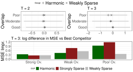
Figure 4: Top panels collect the point estimate (crosses), minus the true effect of the treatment, and confidence intervals of DCB for $p=100$ across the three different designs. The bottom panel reports the decrease in MSE (in logarithmic scale) of the proposed method compared to the best competitor (excluding the one with known propensity score) for $T=3$.

Finally, we report finite sample coverage of the proposed method, DCB in Table 3 for estimating $\mu(\mathbf{1})$ and $\mu(\mathbf{1})-\mu(\mathbf{0})$ (for $T\in\{2,3\}$) in the first two panel with $\eta=0.5$ (see Table 4 in the Appendix for the confidence intervals’ length). The former is of interest when the effect under control is more precise and its variance is asymptotically neglegible compared to the estimated effect under treatment (e.g., many more individuals are not exposed to any treatment). The latter is of interest when both $\mu(1,1)$ and $\mu(0,0)$ are estimated from approximately a proportional sample. In the third panel, we report coverage when instead a Gaussian critical quantile (instead of the square root of a chi-squared quantile discussed in our theorems) is used. We observe that our procedure can lead to correct (over) coverage, while the Gaussian critical quantile leads to under-coverage in the presence of poor overlap and many variables, but correct coverage with fewer variables and two periods only.

We compare DCB and AIPW with high dimensional covariates with a longer time period. Namely, in Figure 5, we collect results for $T\in\{1,\cdots,10\}$. We generate data using a sparse model, $p=100,n=400$ over two-hundred replications. The outcome at time $t$ depends on the contemporaneous treatment, covariates, and previous outcome at time $t-1$. To simulate a scenario where a strong correlation occurs between treatments over a long time period, we generate

$$\mathbb{E}[D_{i,t}|D_{t-1},X_{t}]=(1-\alpha)D_{i,t-1}+\alpha(1+e^{\iota_{i,t}})^{-1},$$

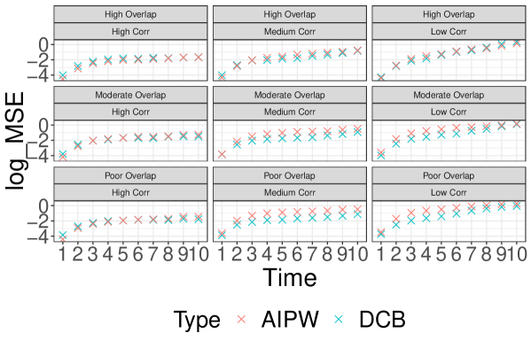
Figure 10: Mean-squared error in log-scale. Simulations for $T\leq 10,p=100,n=400$, two-hundred replications. Here high-correlation denotes strong serial depedence between treatment assignments with $\alpha=0.9$, medium with $\alpha=0.7$ and weak with $\alpha=0.5$. $\eta\in\{0.1,0.3,0.5\}$ for good, moderate and poor overlap, respectively.

where similarly to the propensity score model Equation (18), $\iota_{i,t}=\frac{\eta}{\alpha}X_{i,t-1}\phi+\frac{\eta}{\alpha}X_{i,t}\phi+\frac{1}{2}(D_{i,t-1}-\bar{D}_{t-1})+\xi_{i,t},\xi_{i,t}\sim\mathcal{N}(0,1)$. Here $\eta$ controls overlap together with $\alpha$, where $\eta/\alpha$ has a similar role of the overlap constant in previous simulations. In the figure we report results for $\alpha\in\{0.9,0.7,0.5\}$ (denoted as “High, Medium and Low correlation” respectively), and $\eta\in\{0.3,0.5\}$. In Figure 5, we observe that for very strong time dependence between treatments (i.e., there are limited or no dynamics in assignments) the two methods are comparable. When instead, there are relatively more dynamics in treatment assignments the proposed method significantly improves in mean-squared error, with larger improvements in the presence of poorer overlap. In the Appendix, Figure 10 we provide results also for very good overlap ($\eta=0.1$), where the methods mostly provide comparable results on average.

Finally, in Figure 6 we presents an example of computational time of the method as $T$ varies, showing that the time for $T\leq 10$ is between few seconds and ten minutes on a personal computer. For $T=20$ the computational time is 60 minutes (on a single core, 30 on two cores) in our empirical application.

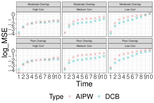
Figure 5: Mean-squared error in log-scale. Simulations for $T\leq 10,p=100,n=400$, two-hundred replications. Here high-correlation denotes strong serial depedence between treatment assignments with $\alpha=0.9$, medium with $\alpha=0.7$ and weak with $\alpha=0.5$. $\eta\in\{0.3,0.5\}$ for moderate and poor overlap, respectively.

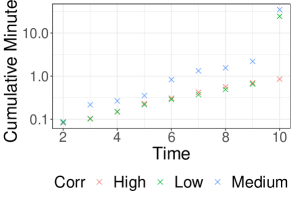
Figure 6: Example of cumulative computational time in minutes to run the first (one) simulation on a personal laptop as $T$ varies High-correlation denotes strong serial dependence between treatments ($\alpha=0.9$), medium corresponds to $\alpha=0.7$ and weak to $\alpha=0.5$. We set $\eta=0.1$.

6.3 Additional numerical studies and misspecified model

In Appendix D we study settings with a misspecified outcome model, low dimensional covariates and settings where the signal of the coefficients decay in the spirit of Wüthrich and Zhu (2023). We show that our findings in the current section are robust to these alternative designs. In particular, in contexts with misspecified models (Appendix D.1) we observe that DCB outperforms AIPW, with a known propensity score. The main reason is due to the instability of the inverse probability weights in dynamic settings. Because these weights define the joint probability of treatment assignments, these can exhibit instability (poor overlap) in small samples, increasing the variance of the AIPW estimator (which we observe in Appendix D.1 as we decompose the bias and variance of each estimator). These findings further motivate the advantages of DCB.

7 Empirical application

In this section, we present an empirical application for studying the effect of democracy on GDP growth using data from Acemoglu et al. (2019). Acemoglu et al. (2019) studied dynamic treatment effects of democracy under GDP growth under sequential ignorability (Assumption 1 in Acemoglu et al., 2019). Figure 7 illustrates the dynamics of treatments. Many units switch treatment over time, violating standard event studies designs, and motivating an approach for dynamic treatments, for example considered in Acemoglu et al. (2019). We revisit the study of Acemoglu et al. (2019) and illustrate the advantages of our method.

7.1 Data and estimation

The data consist of an extensive collection of countries observed between $1960$ and $2010$. We consider observations starting from $1989$. After removing missing values, we run regressions with 141 countries. The outcome is the log-GDP in the country $i$ in period $t$ as in Acemoglu et al. (2019). We use the same treatment specification as in Acemoglu et al. (2019), which is binary and constructed using a political index. We study the effect of exposing countries at time $t$ to democracy for in $s$ years before (and including) $t$ versus not exposing them to democracy for the previous $s$ years. Namely, the estimand is the $s$-long run effect of democracy, after averaging over past assignments as discussed in Section 5. We let $s\in\{1,\cdots,20\}$ to study the impact from one to twenty years of democracy.

For each country, we condition on lag outcomes in the past four years as in the preferred specification of Acemoglu et al. (2019), and past four treatments. We consider a pooled regression (see Section 5) and two alternative specifications. The first is parsimonious and includes dummies for different regions (continents) and different intercepts for different periods. Note that, similarly to what discussed in Zubizarreta (2015), even with a parsimonious specification, residual balancing can substantially improve the finite sample performance of the estimator, as we show in the right panel of Figure 8. The second one controls for the past four outcomes, past four treatments, for the geographical region, and histories based on colonial history and regimes types as defined in the data from Acemoglu et al. (2019). Note that our specification does not include country fixed effects, as our (and Robins (1986)’s) framework assumes that treatments are exogenous conditional on past information. To control for confounding bias that may arise from country specific characteristics (and time) our second specification controls for a large vector of country’s characteristics. We therefore see our second specification as more robust to possible confounding mechanisms. Coefficients are estimated as in Algorithm 1 with model $=$ linear.

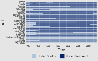
Figure 7: The left panel illustrates the dynamics of treatments. The right panel provides an example of dynamic selection into treatment where treatments may depend on past treatments, outcomes and other past observables (allowed in our framework).

7.2 Results

Figure 8 collects our results. Democracy has a statistically insignificant effect over the first few years and a statistically significant positive impact on long-run GDP growth after six years. Point estimates are in sign and magnitude consistent with what found by Acemoglu et al. (2019), and results are robust across the two specifications for DCB.

We compare our method to three alternative specifications: (i) the AIPW method that uses the same estimation method we propose in Algorithm 1 for estimating the conditional mean function, and the propensity score via penalized generalized linear models as in Negahban et al. (2012); (ii) the linear estimator reported by Acemoglu et al. (2019) (Table 2, Column 3), where dynamic effects are estimated by propagating the effect over past outcomes at each period, as suggested by Acemoglu et al. (2019); the simple local projection, that projects the outcome on the treatment and the past outcome $s$ periods before, controlling for country, time fixed effects and lagged outcome at time $s$ (this specification follows similarly to the regression specifications in macro-economic applications as in Auerbach et al., 2020).

The simple local projection approach reports the smallest point estimates compared to all methods. This result is consistent with our theoretical discussion: local projections average over the distribution of future assignments. Therefore, the causal effects estimated by the local projection differ from the target long-run effect, which instead fixes future treatment assignments. This difference illustrates the benefits of recursive projections in the presence of dynamic selection into treatment, when the goal is to estimate long-run treatment effects. The effect estimated as in Acemoglu et al. (2019) is larger than the local projection method but significantly smaller than the effect estimated through DCB. Therefore, the specification in Acemoglu et al. (2019) may capture some but not all the long-run effects. After controlling for imbalance with DCB, average treatment effects are twice as large. To investigate differences with (A)IPW methods, the right panel in Figure 8 presents comparisons in terms of the imbalance over the lagged outcome at time $t-1$ when using balancing or inverse probability weights. As Acemoglu et al. (2019) note, “Besides controlling for the fact that democratizations are more frequent after economic crises, the lags of GDP per capita summarize the impact of a range of economic factors that affect both growth and democracy, such as commodity prices, agricultural productivity, and technology. Indeed, many of these economic factors should have an impact on future GDP, primarily through their influence on current GDP.” Therefore, an imbalance in lagged GDP may suggest the presence of bias. We report the relative improvement in absolute imbalance (average across the potential outcomes under treatment and control) and observe substantial gain over using inverse probability weights. Such gains illustrate the advantage of balancing in small sample. Finally, Figure 9 complements Figure 8 showing instability of inverse probability weights.

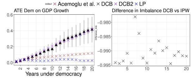
Figure 8: Effect of democracy on economic growth. Left-hand side: pooled regression from $t\in\{1989,\cdots,2010\}$ Gray region denotes the $90\%$ confidence band for the least parsimonious model, with light-gray corresponding to the $\sqrt{\chi_{2T}(\alpha)}$ critical quantile, and darker area to the Gaussian critical quantile. DCB and DCB2 refer to two separate specification, with DCB corresponding to the more parsimonious one. LP denotes a local projection on $t$ periods before, controlling for country, time fixed effects and past outcomes. Right-hand side reports $\log(|I(dcb)|+1)/\log(|I(aipw)|+1)-1\approx|I(dcb)|/|I(aipw)|-1$, where $I(\cdot)$ denotes the imbalance (as in Lemma 3.1) in the lagged outcome using either the DCB weights or IPW weights.

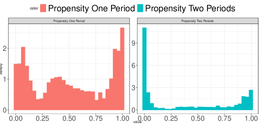
Figure 9: Estimated probability of treatment for one year (left-panel) and two consec- utive years (right-panel). Estimation is performed via logistic regression with a pooled regression with year, region fixed effects and four lagged outcomes. The right panel also controls for the past treatment assignment. The figure illustrates the sensitivity of inverse probability weights to longer time horizon, motivating more stable balancing weights.

8 Discussion

This paper studies the problem of inference on dynamic treatments via covariate balancing. We consider a potential local projection model with high-dimensional covariates, and we introduce novel balancing conditions that allow for the optimal $\sqrt{n}$-consistent estimation. Simulations and empirical applications illustrate the method’s advantages.

Several questions remain open. First, the asymptotic properties crucially rely on cross-sectional independence while allowing for general dependence over time. Future work should addres extensions where cross-sectional $i.i.d.$-ness does not necessarily hold. Second, our asymptotic results assume a fixed period. Future work should study settings with large $T$ (see e.g., Section 5). It would also be interesting to study whether conditions on overlap might be replaced by alternative (weaker) assumptions.

Finally, dynamic treatment regimes and parallel trends impose different (and complementary) assumptions for causal inference. Reconciling these two frameworks and proposing methods that are robust to either condition remains an open research question.

We organize the Appendix as follows. In Appendix A, we present the main lemmas (including sufficient conditions for the convergence rate of lasso). We present proofs of the algorithms in Appendix B. Appendix C presents additional algorithms. Appendix D presents additional simulations, and Appendix E an additional empirical application.

Throughout our discussion, we say that $y\lesssim x$ if the left-hand side is less or equal to the right-hand side up to a multiplicative constant term. We will refer to $\beta^{t}$ as $\beta^{(t)}_{d_{1:T}}$ whenever clear from the context. Recall that when we omit the script $i$, we refer to the vector of all observations. We define

$$\nu_{i,t}(d_{1:T})=H_{i,t+1}\beta^{(t+1)}_{d_{1:T}}-H_{i,t}\beta^{(t)}_{d_{1:T}},\quad\varepsilon_{i,T}(d_{1:T})=Y_{i,T}(d_{1:T})-H_{i,T}\beta_{d_{1:T}}^{(T)}.$$

and $\hat{\nu}_{i,t}$ for estimated coefficients (omitting the argument $(d_{1:T})$ for notational convenience). Let $\nu_{i,0}=X_{i,1}\beta^{1}-\mathbb{E}[X_{i,1}]\beta^{1}$ and $\hat{\nu}_{i,0}=X_{i,1}\hat{\beta}^{1}-\bar{X}_{1}\hat{\beta}^{1}$. We will refer to $\hat{\gamma}_{i,t}(d_{1:T})$ as the weights to estimate $\mu_{T}(d_{1:T})$ as in Algorithm 3. We omit the argument $d_{1:T}$ in $\hat{\gamma}_{i,t}(\cdot),\nu_{i,t}(\cdot)$ whenever clear from the context. We denote $\sigma(X)$ the sigma-algebra generated by a random variable $X$.

Appendix A Lemmas

A.1 Proof of Lemma 2.1

The first equation in Lemma 2.1 is a direct consequence of condition (A) in Assumption 2, and the linear model assumption (Assumption 3). Consider the second equation in Lemma 2.1. By condition (B) in Assumption 2, we have

$$\mathbb{E}\Big{[}Y_{i,2}(d_{1},d_{2})\Big{|}X_{i,1}\Big{]}=\mathbb{E}\Big{[}Y_{i,2}(d_{1},d_{2})\Big{|}X_{i,1},D_{i,1}=d_{1}\Big{]}.$$

Using the law of iterated expectations (since $X_{i,1}$ is measurable with respect to $H_{i,2}$)

$$\mathbb{E}\Big{[}Y_{i,2}(d_{1},d_{2})\Big{|}X_{i,1},D_{i,1}=d_{1}\Big{]}=\mathbb{E}\Big{[}\mathbb{E}[Y_{i,2}(d_{1},d_{2})|H_{i,2},D_{i,1}=d_{1}]|X_{i,1},D_{i,1}=d_{1}\Big{]}.$$

Using condition (A) in Assumption 2, we have

$$\mathbb{E}[Y_{i,2}(d_{1},d_{2})|H_{i,2},D_{i,1}=d_{1}]=\mathbb{E}[Y_{i,2}(d_{1},d_{2})|H_{i,2},D_{i,1}=d_{1},D_{i,2}=d_{2}]$$

the proof completes as $\mathbb{E}[Y_{i,2}(d_{1},d_{2})|H_{i,2},D_{i,1}=d_{1},D_{i,2}=d_{2}]=\mathbb{E}[Y_{i,2}|H_{i,2},D_{i,1}=d_{1},D_{i,2}=d_{2}]$ as a consequence of condition (A) in Assumption 2.

A.2 Proof of Lemma 4.1

We prove the main lemmas for multiple periods as the two-periods case is a special case.

Throughout the proof we omit the argument $d_{1:T}$ of $\hat{\gamma}_{t}(d_{1:T})$ for notational convenience. Recall that $\hat{\gamma}_{i,T}=0$ if $D_{i,1:T}\neq d_{1:T}$. Therefore,

$$\hat{\gamma}_{i,T}Y_{i,T}=\hat{\gamma}_{i,T}Y_{i,T}(d_{1:T})=\hat{\gamma}_{i,T}(H_{i,T}\beta_{d_{1:T}}^{T}+\varepsilon_{i,T}).$$

We can write

$$\sum_{i=1}^{n}\Big{(}\hat{\gamma}_{i,T}Y_{i,T}-\sum_{t=2}^{T}(\hat{\gamma}_{i,t}-\hat{\gamma}_{i,t-1})H_{i,t}\hat{\beta}_{d_{1:T}}^{t}-(\hat{\gamma}_{i,1}-\frac{1}{n})X_{i,1}\hat{\beta}_{d_{1:T}}^{1}\Big{)}$$

$$=\sum_{i=1}^{n}\Big{(}\hat{\gamma}_{i,T}H_{i,T}\beta_{d_{1:T}}^{T}-\sum_{t=2}^{T}(\hat{\gamma}_{i,t}-\hat{\gamma}_{i,t-1})H_{i,t}\hat{\beta}_{d_{1:T}}^{t}-(\hat{\gamma}_{i,1}-\frac{1}{n})X_{i,1}\hat{\beta}_{d_{1:T}}^{1}\Big{)}+\hat{\gamma}_{T}^{\top}\varepsilon_{T}.$$

Consider first the term

$$\sum_{i=1}^{n}(\hat{\gamma}_{i,T}H_{i,T}\beta_{d_{1:T}}^{T}-(\hat{\gamma}_{i,T}-\hat{\gamma}_{i,T-1})H_{i,T}\hat{\beta}_{d_{1:T}}^{T})=(\hat{\gamma}_{T}H_{T}-\hat{\gamma}_{T-1}H_{T})(\beta_{d_{1:T}}^{T}-\hat{\beta}_{d_{1:T}}^{T})+\hat{\gamma}_{T-1}H_{T}\beta_{d_{1:T}}^{T}.$$

For any $s>1$,

$$\sum_{i=1}^{n}(\hat{\gamma}_{i,s}-\hat{\gamma}_{i,s-1})H_{i,s}\hat{\beta}_{d_{1:T}}^{s}=(\hat{\gamma}_{s}H_{s}-\hat{\gamma}_{s-1}H_{s})(\hat{\beta}_{d_{1:T}}^{s}-\beta_{d_{1:T}}^{s})+\hat{\gamma}_{s}H_{s}\beta_{d_{1:s}}^{s}-\hat{\gamma}_{s-1}H_{s}\beta_{d_{1:s}}^{s}.$$

For $s=1$, it follows

$$\sum_{i=1}^{n}(\hat{\gamma}_{i,1}-\frac{1}{n})X_{i,1}\hat{\beta}_{d_{1:T}}^{1}=(\hat{\gamma}_{1}X_{1}-\bar{X}_{1})(\hat{\beta}_{d_{1:T}}^{1}-\beta_{d_{1:T}}^{1})+\hat{\gamma}_{1}X_{1}\beta_{d_{1:s}}^{1}-\bar{X}_{1}\beta_{d_{1:s}}^{1}.$$

Therefore, we can write

$$\sum_{i=1}^{n}\Big{(}\hat{\gamma}_{i,T}Y_{i,T}-\sum_{t=2}^{T}(\hat{\gamma}_{i,t}-\hat{\gamma}_{i,t-1})H_{i,t}\hat{\beta}_{d_{1:T}}^{t}-(\hat{\gamma}_{i,1}-\frac{1}{n})X_{i,1}\hat{\beta}_{d_{1:T}}^{1}\Big{)}$$

$$=(\hat{\gamma}_{T}H_{T}-\hat{\gamma}_{T-1}H_{T})(\beta_{d_{1:T}}^{T}-\hat{\beta}_{d_{1:T}}^{T})+\sum_{s=2}^{T-1}(\hat{\gamma}_{s}H_{s}-\hat{\gamma}_{s-1}H_{s})(\beta_{d_{1:T}}^{s}-\hat{\beta}_{d_{1:T}}^{s})+(\hat{\gamma}_{1}X_{1}-\bar{X}_{1})(\beta_{d_{1:T}}^{1}-\hat{\beta}_{d_{1:T}}^{1})$$

$$+\hat{\gamma}_{T}H_{T}\beta_{d_{1:T}}^{T}+\gamma_{T}^{\top}\varepsilon_{T}-\Big{[}\sum_{s=2}^{T-1}\hat{\gamma}_{s+1}H_{s}\beta_{d_{1:s}}^{s}-\hat{\gamma}_{s}H_{s}\beta_{d_{1:s}}^{s}\Big{]}-\hat{\gamma}_{1}X_{1}\beta_{d_{1:s}}^{1}+\bar{X}_{1}\beta_{d_{1:s}}^{1}.$$

The proof completes after collecting the desired terms.

A.3 Proof of Lemma 4.2

Since $\hat{\gamma}_{i,t}(d_{1:T})$ is equal to zero if $D_{i,1:t}\neq d_{1:t}$ we can focus to the case where $D_{i,1:t}=d_{1:t}$. Since weights at time $t-1$ are measurable with respect to $\mathcal{F}_{t-1},D_{t-1}$, we only need to show

$$\mathbb{E}[\hat{\gamma}_{i,t-1}(d_{1:T})H_{t}\beta_{d_{1:T}}^{t}|\mathcal{F}_{t-1},D_{-i,t-1},D_{i,(1:(t-1))}=d_{1:(t-1)}]=\hat{\gamma}_{i,t}(d_{1:T})H_{t-1}\beta_{d_{1:T}}^{t-1}.$$ (19)

On the event that $D_{i,(1:(t-1))}\neq d_{1:(t-1)}$ the expression is zero on both sides and the result trivially holds. Therefore, we can implicitely assume that $D_{i,(1:(t-1))}=d_{1:(t-1)}$ since otherwise the result trivially holds. Under Assumption 4 we can write

$$\mathbb{E}[\hat{\gamma}_{i,t-1}(d_{1:T})H_{t}\beta_{d_{1:T}}^{t}|\mathcal{F}_{t-1},D_{t-1}] =\mathbb{E}\Big{[}\hat{\gamma}_{i,t-1}(d_{1:T})\mathbb{E}[Y_{i,T}(d_{1:T})|\mathcal{F}_{t},D_{t}]\Big{|}\mathcal{F}_{t-1},D_{t-1}\Big{]}$$ (20)

$$=\hat{\gamma}_{i,t-1}(d_{1:T})\mathbb{E}[Y_{i,T}(d_{1:T})|\mathcal{F}_{t-1},D_{t-1}]$$

by the tower property of the expectation and the definition of $\mathcal{F}_{t}$. Now notice that under Assumption 4 (B), $\begin{aligned} \mathbb{E}[Y_{i,T}(d_{1:T})|\mathcal{F}_{t-1},D_{t-1}]=\mathbb{E}[Y_{i,T}(d_{1:T})|\mathcal{F}_{t-1}].\end{aligned}$ Therefore

$$\hat{\gamma}_{i,t-1}(d_{1:T})\mathbb{E}[Y_{i,T}(d_{1:T})|\mathcal{F}_{t-1}]=\hat{\gamma}_{i,t-1}(d_{1:T})H_{i,t-1}\beta_{d_{1:(t-1)}}^{t-1}.$$ (21)

A.4 Sufficient conditions for lasso

In this section we provide sufficient conditions for the convergence rate of lasso in two periods as in Assumption 6 (i). $T$-periods follows similarly.

Lemma A.1 (Sufficient conditions for Lasso).

Suppose that $||H_{2}||_{\infty},||X_{1}||_{\infty}$ are uniformly bounded almost surely and $||\beta_{d_{1:2}}^{(2)}||_{0},||\beta_{d_{1:2}}^{(1)}||_{0}\leq s,||\beta_{d_{1:2}}^{(2)}||_{\infty},||\beta_{d_{1:2}}^{(1)}||_{\infty}\leq s$. Suppose that $H_{2},X_{1}$ both satisfy the restricted eigenvalue assumption, and the column normalization condition (Negahban et al., 2012). Suppose that $\hat{\beta}_{d_{1:2}}^{(1)},\hat{\beta}_{d_{1:2}}^{(2)}$ are estimated with Lasso as in Algorithm 1 with a full interaction model and with penalty parameter $\lambda_{n}\asymp s\sqrt{\log(p)/n}$. Let Assumptions 1 - 3 hold. Let $\varepsilon_{2}(d_{1:2})|H_{2}$ be subgaussian almost surely and $\nu_{1}(d_{1})|X_{1}$ be sub-gaussian almost surely. Then for $t\in\{1,2\}$,

$$\Big{|}\Big{|}\hat{\beta}_{d_{1:2}}^{(t)}-\beta_{d_{1:2}}^{(t)}\Big{|}\Big{|}_{1}=\mathcal{O}_{p}\Big{(}s^{2}\sqrt{\log(p)/n}\Big{)}.$$

Therefore,

$$\|\hat{\beta}_{d_{1:2}}^{(t)}-\beta_{d_{1:2}}^{(t)}\|_{1}\delta_{t}(n,p)=o_{p}(1/\sqrt{n}),$$

for $\delta_{t}(n,p)\asymp\log(np)/n^{1/4}$ and $s^{2}\log^{3/2}(np)/n^{1/4}=\mathcal{O}(1)$.

The proof is discussed below and follows similarly to Negahban et al. (2012), with minor modifications. The above result provides a set of sufficient conditions such that Assumption 6 (i) holds for a feasible choice of $\delta_{t}$. Interestingly, the estimation error propagates each period through stricter restrictions on the sparsity parameter $s$ compared to the standard lasso method (whose error scales with $\sqrt{s}$ instead of $s$). The reason is because of the recursive approach.

Proof.

The result for

$$\Big{|}\Big{|}\hat{\beta}_{d_{1:2}}^{2}-\beta_{d_{1:2}}^{2}\Big{|}\Big{|}_{1}=\mathcal{O}_{p}\Big{(}s\sqrt{\log(p)/n}\Big{)}$$

follows verbatim from Negahban et al. (2012) Corollary 2. For the result for $\hat{\beta}_{d_{1:2}}^{1}$ it suffices to notice, following the same argument from Negahban et al. (2012) (Corollary 2), that

$$\Big{|}\Big{|}\hat{\beta}_{d_{1:2}}^{1}-\beta_{d_{1:2}}^{1}\Big{|}\Big{|}_{1}=O(s\lambda_{n}),\text{ for }\lambda_{n}\geq\Big{|}\Big{|}\frac{1}{n}X_{1}^{\top}(H_{2}\hat{\beta}_{d_{1:2}}^{2}-X_{1}\beta_{d_{1:2}}^{1})\Big{|}\Big{|}_{\infty},$$

since here we used the estimated outcome $H_{2}\hat{\beta}_{d_{1:T}}^{2}$ as the outcome of interest in our estimated regression instead of the true outcome. The upper bound as a function of $\lambda_{n}$ follows directly from Theorem 1 in Negahban et al. (2012). We note that we can write

$$\Big{|}\Big{|}\frac{1}{n}X_{1}^{\top}(H_{2}\hat{\beta}_{d_{1:2}}^{2}-X_{1}\beta_{d_{1:2}}^{1})\Big{|}\Big{|}_{\infty} \leq\Big{|}\Big{|}\frac{1}{n}X_{1}^{\top}\nu_{1}\Big{|}\Big{|}_{\infty}+\Big{|}\Big{|}\frac{1}{n}X_{1}^{\top}(H_{2}\hat{\beta}_{d_{1:2}}^{2}-H_{2}\beta_{d_{1:2}}^{2})\Big{|}\Big{|}_{\infty}$$

$$=\Big{|}\Big{|}\frac{1}{n}X_{1}^{\top}\nu_{1}\Big{|}\Big{|}_{\infty}+\Big{|}\Big{|}\frac{1}{n}X_{1}^{\top}H_{2}(\beta_{d_{1:2}}^{2}-\hat{\beta}_{d_{1:2}}^{2})\Big{|}\Big{|}_{\infty}$$

$$\leq\Big{|}\Big{|}\frac{1}{n}X_{1}^{\top}\nu_{1}\Big{|}\Big{|}_{\infty}+||X_{1}||_{\infty}||H_{2}||_{\infty}||\beta_{d_{1:2}}^{2}-\hat{\beta}_{d_{1:2}}^{2}||_{1}.$$

We now study each component separately. By sub-gaussianity, since $\mathbb{E}[\nu_{1}|X_{1}]=0$ by Assumption 3, we have for all $t>0$, by Hoeffding inequality and the union bound,

$$P\Big{(}\Big{|}\Big{|}\frac{1}{n}X_{1}^{\top}\nu_{1}\Big{|}\Big{|}_{\infty}>t\Big{|}X_{1}\Big{)}\leq p\exp\Big{(}-M\frac{t^{2}n}{s}\Big{)}$$

for a finite constant $M$. This result follows since $\nu_{1}\leq||\beta_{1}||_{1}||X_{1}^{(j)}||_{\infty}\leq Ms$. It implies that

$$\Big{|}\Big{|}\frac{1}{n}X_{1}^{\top}\nu_{1}\Big{|}\Big{|}_{\infty}=O_{p}(\sqrt{s\log(p)/n})$$

The second component instead is $O_{p}(s\sqrt{\log(p)/n})$ by the bound on $||\beta_{d_{1:2}}^{2}-\hat{\beta}_{d_{1:2}}^{2}||_{1}$. This complete the proof. Finally, observe also that the same argument follows recursively for any finite $T$, with the estimation error depending on $T$. ∎

A.5 Auxiliary Lemmas

In the lemmas below we will refer to $a,c_{0},C$ as finite constants.

Lemma A.2 (Existence of Feasible $\hat{\gamma}_{1}$).

Suppose that $X_{i,1}^{(j)}$ is subgaussian for all $j\in\{1,\cdots,p_{1}\}$, $X_{i,1}\in\mathbb{R}^{p_{1}}$. Suppose that for $d_{1}\in\{0,1\}$, $P(D_{i,1}=d_{1}|X_{i,1})\in(\delta,1-\delta)$, for some $\delta\in(0,1)$. For finite constants $c_{0},C<\infty$, with probability at least $1-5/n$, for $\log(2np_{1})/n\leq c_{0}$, $\delta_{1}(n,p_{1})\geq C\sqrt{2\log(2np_{1})/n}$, there exists a feasible $\hat{\gamma}_{1}$ solving Algorithm 3. In addition,

$$\lim_{n\rightarrow\infty}P\Big{(}n||\hat{\gamma}_{1}||_{2}^{2}\leq\mathbb{E}\Big{[}\frac{1}{P(D_{i,1}=d_{1}|X_{i,1})}\Big{]}\Big{)}=1.$$

Proof of Lemma A.2.

This proof follows similarly to the one-period setting in Athey et al. (2018).

Feasible guess

To prove existence of a feasible weight, we use a feasible guess. We prove the claim for a general $d_{1}\in\{0,1\}$. Consider first

$$\hat{\gamma}_{i,1}^{*}=\frac{1\{D_{i,1}=d_{1}\}}{nP(D_{i,1}=d_{1}|X_{i,1})}\Big{/}\underbrace{\Big{(}\frac{1}{n}\sum_{i=1}^{n}\frac{1\{D_{i,1}=d_{1}\}}{P(D_{i,1}=d_{1}|X_{i,1})}\Big{)}}_{(D)}.$$ (22)

(D) is bounded away from zero

For the guess in Equation (22) to be well-defined, we need that the denominator is bounded away from zero. We now provide bounds on the denominator. Since $P(D_{i,1}=d_{1}|X_{i,1})\in(\delta,1-\delta)$ by Hoeffding inequality

$$P\Big{(}\Big{|}\frac{1}{n}\sum_{i=1}^{n}\frac{1\{D_{i,1}=d_{1}\}}{P(D_{i,1}=d_{1}|X_{i,1})}-1\Big{|}>t\Big{)}\leq 2\exp\Big{(}-\frac{nt^{2}}{2a^{2}}\Big{)},$$

for a finite constant $a$ that only depends on the overlap constant $\delta$. With probability at least $1-1/n$,

$$\frac{1}{n}\sum_{i=1}^{n}\frac{1\{D_{i,1}=d_{1}\}}{P(D_{i,1}=d_{1}|X_{i,1})}>1-\sqrt{2a^{2}\log(2n)/n}.$$ (23)

Therefore for $n$ large enough such that $\sqrt{2a^{2}\log(2n)/n}<1-\kappa$, taking some $\kappa\in(0,1)$, weights are finite with probability at least $1-1/n$.

Weights sum up to one and satisfies $\mathcal{O}(n^{-2/3})$ constraint

The weights in Equation (22) sum up to one and with probability at least $1-1/n$

$$\frac{1\{D_{i,1}=d_{1}\}}{nP(D_{i,1}=d_{1}|X_{i,1})}\lesssim n^{-2/3}\Rightarrow\gamma_{i,1}^{*}\leq K_{2,1}n^{-2/3}$$

for a constant $K_{2,1}$, where the first inequality follows by the overlap assumption that $P(D_{i,1}=d_{1}|X_{i,1})\in(\delta,1-\delta)$, and the second by Equation (23).

First constraint in Algorithm 3

We are left to show that the first constraint in Algorithm 3 is satisfied.

Under Assumption 4, $\mathbb{E}\Big{[}\frac{1}{n}\sum_{i=1}^{n}\frac{1\{D_{i,1}=d_{1}\}X_{i,1}^{(j)}}{P(D_{i,1}=1|X_{i,1})}|X_{1}\Big{]}=\bar{X}_{1}^{(j)}.$ In addition, since $X_{i,1}$ is subgaussian, and $1/P(D_{i,1}=d_{1}|X_{i,1})$ is uniformly bounded,

$$P\Big{(}\Big{|}\Big{|}\bar{X}_{1}-\frac{1}{n}\sum_{i=1}^{n}\frac{1\{D_{i,1}=d_{1}\}}{P(D_{i,1}=1|X_{i,1})}X_{i,1}\Big{|}\Big{|}_{\infty}>t\Big{)}\leq p_{1}2\exp\Big{(}-\frac{nt^{2}}{2a^{2}}\Big{)}$$

for a finite constant $a^{2}$. With trivial rearrangement, with probability $1-1/n$,

$$\Big{|}\Big{|}\bar{X}_{1}-\frac{1}{n}\sum_{i=1}^{n}\frac{1\{D_{i,1}=d_{1}\}}{P(D_{i,1}=1|X_{i,1})}X_{i,1}\Big{|}\Big{|}_{\infty}\leq a\sqrt{2\log(2np)/n}$$ (24)

Consider now the denominator $(D)$ in Equation (22). We have shown that with probability $1-1/n$, for a finite constant $a<\infty$,

$$\Big{|}\frac{1}{n}\sum_{i=1}^{n}\frac{1\{D_{i,1}=d_{1}\}}{P(D_{i,1}=d_{1}|X_{i,1})}-1\Big{|}\leq 2a\sqrt{\log(2n)/n}.$$ (25)

Therefore, with probability $1-2/n$,

$$\Big{|}\Big{|}\bar{X}_{1}-\frac{\frac{1}{n}\sum_{i=1}^{n}\frac{1\{D_{i,1}=d_{1}\}}{P(D_{i,1}=1|X_{i,1})}X_{i,1}}{\frac{1}{n}\sum_{i=1}^{n}\frac{1\{D_{i,1}=d_{1}\}}{P(D_{i,1}=1|X_{i,1})}}\Big{|}\Big{|}_{\infty}=\Big{|}\Big{|}\frac{\bar{X}_{1}\frac{1}{n}\sum_{i=1}^{n}\frac{1\{D_{i,1}=d_{1}\}}{P(D_{i,1}=1|X_{i,1})}-\frac{1}{n}\sum_{i=1}^{n}\frac{1\{D_{i,1}=d_{1}\}}{P(D_{i,1}=1|X_{i,1})}X_{i,1}}{\frac{1}{n}\sum_{i=1}^{n}\frac{1\{D_{i,1}=d_{1}\}}{P(D_{i,1}=1|X_{i,1})}}\Big{|}\Big{|}_{\infty}$$ (26)

$$\qquad=\Big{|}\Big{|}\frac{\bar{X}_{1}\frac{1}{n}\sum_{i=1}^{n}\frac{1\{D_{i,1}=d_{1}\}}{P(D_{i,1}=1|X_{i,1})}+\bar{X}_{1}-\bar{X}_{1}-\frac{1}{n}\sum_{i=1}^{n}\frac{1\{D_{i,1}=d_{1}\}}{P(D_{i,1}=1|X_{i,1})}X_{i,1}}{\frac{1}{n}\sum_{i=1}^{n}\frac{1\{D_{i,1}=d_{1}\}}{P(D_{i,1}=1|X_{i,1})}}\Big{|}\Big{|}_{\infty}$$

$$\qquad\leq\Big{|}\Big{|}\frac{\bar{X}_{1}-\frac{1}{n}\sum_{i=1}^{n}\frac{1\{D_{i,1}=d_{1}\}}{P(D_{i,1}=1|X_{i,1})}X_{i,1}}{\frac{1}{n}\sum_{i=1}^{n}\frac{1\{D_{i,1}=d_{1}\}}{P(D_{i,1}=1|X_{i,1})}}\Big{|}\Big{|}_{\infty}+\frac{2a\sqrt{\log(2n)/n}}{\frac{1}{n}\sum_{i=1}^{n}\frac{1\{D_{i,1}=d_{1}\}}{P(D_{i,1}=1|X_{i,1})}}$$

$$\qquad\leq\frac{a\sqrt{2\log(2np)/n}+2a\sqrt{\log(2n)/n}}{\frac{1}{n}\sum_{i=1}^{n}\frac{1\{D_{i,1}=d_{1}\}}{P(D_{i,1}=1|X_{i,1})}},$$

where the first inequality follows by the triangular inequality and by concentration of the term $\frac{1}{n}\sum_{i=1}^{n}\frac{1\{D_{i,1}=d_{1}\}}{P(D_{i,1}=1|X_{i,1})}$ around one at exponential rate as in Equation (25). The second inequality follows by concentration of the numerator as in Equation (24). With probability $1-1/n$, the denominator $(D)$ is bounded away from zero. Therefore for a universal constant $C<\infty$,

$$\small P\Big{(}\Big{|}\Big{|}\bar{X}_{1}-\frac{\frac{1}{n}\sum_{i=1}^{n}\frac{1\{D_{i,1}=d_{1}\}}{P(D_{i,1}=1|X_{i,1})}X_{i,1}}{\frac{1}{n}\sum_{i=1}^{n}\frac{1\{D_{i,1}=d_{1}\}}{P(D_{i,1}=1|X_{i,1})}}\Big{|}\Big{|}_{\infty}\leq Ca\sqrt{2\log(2np)/n}\Big{)}\geq 1-3/n.$$ (27)

Bound on $||\hat{\gamma}||_{2}^{2}$

We are left to provide bounds on $||\hat{\gamma}_{1}||_{2}^{2}$. For $n$ large enough, with probability at least $1-5/n$, $||\hat{\gamma}_{1}||_{2}^{2}\leq||\hat{\gamma}_{1}^{*}||_{2}^{2}$ since $\hat{\gamma}_{1}^{*}$ is a feasible solution. By overlap, the fourth moment of $1/P(D_{i,1}=d_{1}|X_{i,1})$ is bounded. By the strong law of large numbers and Slutsky theorem,

$$n||\hat{\gamma}_{1}^{*}||_{2}^{2} =\sum_{i=1}^{n}\frac{1\{D_{i,1}=d_{1}\}}{nP(D_{i,1}=d_{1}|X_{i,1})^{2}}\Big{/}\Big{(}\sum_{i=1}^{n}\frac{1\{D_{i,1}=d_{1}\}}{nP(D_{i,1}=d_{1}|X_{i,1})}\Big{)}^{2}\rightarrow_{as}\frac{\mathbb{E}[\frac{1\{D_{i,1}=d_{1}\}}{P(D_{i,1}=d_{1}|X_{i,1})^{2}}]}{\mathbb{E}[\frac{1\{D_{i,1}=d_{1}\}}{P(D_{i,1}=d_{1}|X_{i,1})}]^{2}}<\infty.$$ (28)

which completes the proof. ∎

Lemma A.3 (Existence of a feasible $\hat{\gamma}_{t}$).

Let

$$Z_{i,t}(d_{t})=\frac{1\{D_{i,t}=d_{t}\}}{P(D_{i,t}=d_{t}|Y_{i,1},\cdots,Y_{i,t-1},X_{i,1},\cdots,X_{i,t-1},D_{i,1},\cdots,D_{i,t-1})}.$$

Let Assumption 5 hold and let for finite constants $c_{0},\bar{c}$,

$$\delta_{t}(n,p_{t})\geq c_{0}\frac{\log^{3/2}(p_{t}n)}{n^{1/2}},\quad\mbox{and}\quad K_{2,t}=2K_{2,t-1}\bar{c}.$$

Then with probability $\eta_{n}\rightarrow 1$, for some $N>0$, $n\geq N$, there exists a feasible $\hat{\gamma}_{t}^{*}$ solving the optimization in Algorithm 3, where

$$\hat{\gamma}_{i,t}^{*}=\hat{\gamma}_{i,t-1}Z_{i,t}(d_{t})\Big{/}\sum_{i=1}^{n}\hat{\gamma}_{i,t-1}Z_{i,t}(d_{t})$$

In addition,

$$\lim_{n\rightarrow\infty}P\Big{(}n||\hat{\gamma}_{t}||_{2}^{2}\leq C_{t}\Big{)}=1$$ (29)

for a constant $1\leq C_{t}<\infty$ independent of $(p_{t},n)$.

Proof of Lemma A.3.

The proof follows by induction. By Lemma A.2 we know that there exist a feasible $\hat{\gamma}_{1}$, with $\lim_{n\rightarrow\infty}P(n||\hat{\gamma}_{1}||_{2}^{2}\leq C_{1})=1$, for some finite $C_{1}<\infty$. Suppose now that there exist feasible $\hat{\gamma}_{1},...,\hat{\gamma}_{t-1}$, such that

$$\lim_{n\rightarrow\infty}P(n||\hat{\gamma}_{s}||_{2}^{2}\leq C_{s})=1$$ (30)

for some finite constant $C_{s}<\infty$ depends on $s$, and for all $s<t$. We want to show that the statement holds for $\hat{\gamma}_{t}$. We find $\gamma_{t}^{*}$ that satisfies the constraint, with

$$\hat{\gamma}_{i,t}^{*}=\hat{\gamma}_{i,t-1}\frac{1\{D_{i,t}=d_{t}\}}{P(D_{i,t}=d_{t}|H_{i,t})}\Big{/}\Big{(}\sum_{i=1}^{n}\hat{\gamma}_{i,t-1}\frac{1\{D_{i,t}=d_{t}\}}{P(D_{i,t}=d_{t}|H_{i,t})}\Big{)}.$$ (31)

We break the proof into several steps.

Finite and Bounded Weights

To show that such weights are finite, with high probability, we need to impose bounds on the numerator and the denominator of the weights in Equation (31). We want to bound for a finite constant $\bar{C}<\infty$,

$$P\Big{(}\Big{\{}\max_{i\in\{1,...,n\}}\hat{\gamma}_{i,t-1}\frac{1\{D_{i,t}=d_{t}\}}{P(D_{i,t}=d_{t}|H_{i,t})}>\bar{C}n^{-2/3}K_{2,t-1}\Big{\}}\bigcup\Big{\{}\sum_{i=1}^{n}\hat{\gamma}_{i,t}\frac{1\{D_{i,t}=d_{t}\}}{P(D_{i,t}=d_{t}|H_{i,t})}>\epsilon\Big{\}}\Big{)}$$

$$\leq\underbrace{P\Big{(}\max_{i\in\{1,...,n\}}\hat{\gamma}_{i,t-1}\frac{1\{D_{i,t}=d_{t}\}}{P(D_{i,t}=d_{t}|H_{i,t})}>\bar{C}n^{-2/3}K_{2,t-1}\Big{)}}_{(i)}+\underbrace{P\Big{(}\sum_{i=1}^{n}\hat{\gamma}_{i,t}\frac{1\{D_{i,t}=d_{t}\}}{P(D_{i,t}=d_{t}|H_{i,t})}>\epsilon\Big{)}}_{(ii)}.$$

Bound on $(i)$

We start by $(i)$. Observe first that we can bound

$$\max_{i\in\{1,...,n\}}\hat{\gamma}_{i,t-1}\frac{1\{D_{i,t}=d_{t}\}}{P(D_{i,t}=d_{t}|H_{i,t})}\leq n^{-2/3}K_{2,t-1}\max_{i\in\{1,...,n\}}\frac{1\{D_{i,t}=d_{t}\}}{P(D_{i,t}=d_{t}|H_{i,t})}\leq K_{2,t-1}\bar{C}n^{-2/3}$$

for a finite constant $\bar{C}$ by strong overlap (Assumption 5).

Bound on $(ii)$

We now provide bounds on $(ii)$. Since $\sigma(H_{t-1})\subseteq\sigma(H_{t})$

$$\mathbb{E}\Big{[}\sum_{i=1}^{n}\hat{\gamma}_{i,t-1}\frac{1\{D_{i,t}=d_{t}\}}{P(D_{i,t}=d_{t}|H_{i,t})}\Big{]} =\mathbb{E}\Big{[}\mathbb{E}\Big{[}\sum_{i=1}^{n}\hat{\gamma}_{i,t-1}\frac{1\{D_{i,t}=d_{t}\}}{P(D_{i,t}=d_{t}|H_{i,t})}\Big{|}H_{t-1}\Big{]}\Big{]}$$

$$=\mathbb{E}\Big{[}\sum_{i=1}^{n}\hat{\gamma}_{i,t-1}\mathbb{E}\Big{[}\mathbb{E}\Big{[}\frac{1\{D_{i,t}=d_{t}\}}{P(D_{i,t}=d_{t}|H_{i,t})}\Big{|}H_{t}\Big{]}\Big{|}H_{t-1}\Big{]}\Big{]}=\sum_{i=1}^{n}\hat{\gamma}_{i,t-1}=1.$$

Let $C_{t-1}$ be the upper limit on $n||\hat{\gamma}_{t-1}||_{2}^{2}$, and let

$$c:=1\Big{/}C_{t-1}\quad\eta_{n,t}:=P(||\hat{\gamma}_{t-1}||_{2}^{2}\leq 1/(cn)),$$ (32)

for some constant $c$, which depends on $t-1$ (the dependence with $t-1$ is suppressed for expositional convenience). Observe in addition that $\eta_{n,t}\rightarrow 1$ by the induction argument (see Equation (30)). We write for a finite constant $a$, for any $h>0$

$$P\Big{(}\Big{|}\sum_{i=1}^{n}\hat{\gamma}_{i,t-1}\frac{1\{D_{i,t}=d_{t}\}}{P(D_{i,t}=d_{t}|H_{i,t})}-1\Big{|}>h\Big{)}$$ (33)

$$\leq P\Big{(}\Big{|}\sum_{i=1}^{n}\hat{\gamma}_{i,t-1}\frac{1\{D_{i,t}=d_{t}\}}{P(D_{i,t}=d_{t}|H_{i,t})}-1\Big{|}>h\Big{|}||\hat{\gamma}_{t-1}||_{2}^{2}\leq 1/(cn)\Big{)}\eta_{n,t}+(1-\eta_{n,t})$$

$$\leq 2\exp\Big{(}-\frac{ah^{2}}{2||\hat{\gamma}_{t-1}||_{2}^{2}}\Big{|}||\hat{\gamma}_{t-1}||_{2}^{2}\leq 1/(cn)\Big{)}\eta_{n,t}+(1-\eta_{n,t})$$

$$\leq 2\exp\Big{(}-\frac{ch^{2}an}{2}\Big{)}\eta_{n,t}+(1-\eta_{n,t}).$$

The third inequality follows from the fact that $\hat{\gamma}_{t-1}$ is measurable with respect to $H_{t-1}$ and $\frac{1\{D_{i,t}=d_{t}\}}{P(D_{i,t}=d_{t}|H_{i,t})}$ is sub-gaussian conditional on $H_{i,t-1}$ (since uniformly bounded). Therefore with probability at least $1-\kappa$,

$$\Big{|}\sum_{i=1}^{n}\hat{\gamma}_{i,t-1}\frac{1\{D_{i,t}=d_{t}\}}{P(D_{i,t}=d_{t}|H_{i,t})}-1\Big{|}\leq\sqrt{2\log(2\eta_{n,t}/(\kappa+\eta_{n,t}-1))/(acn)}.$$ (34)

By setting $\kappa=\eta_{n,t}/n+(1-\eta_{n,t})$, with probability at least $1-\eta_{n,t}/n+(1-\eta_{n,t})$,

$$\Big{|}\sum_{i=1}^{n}\hat{\gamma}_{i,t-1}\frac{1\{D_{i,t}=d_{t}\}}{P(D_{i,t}=d_{t}|H_{i,t})}-1\Big{|}\leq\sqrt{2\log(2n)/acn},$$

and hence the denominator is bounded away from zero for $n$ large enough (recall that $\eta_{n,t}\rightarrow 1$ by induction).

First Constraint in Algorithm 3

We now show that the proposed weights in Equation (31) satisfy the first constraint in Algorithm 3. The second constraint trivially holds, while the third follows from the “finite and bounded weights” argument discussed in the paragraph above. We write

$$\mathbb{E}\Big{[}\sum_{i=1}^{n}\hat{\gamma}_{i,t-1}H_{i,t}^{(j)}-\sum_{i=1}^{n}\hat{\gamma}_{i,t-1}\frac{1\{D_{i,t}=d_{t}\}}{P(D_{i,t}=d_{t}|H_{i,t})}H_{i,t}^{(j)}\Big{]}$$

$$=\mathbb{E}\Big{[}\mathbb{E}\Big{[}\sum_{i=1}^{n}\hat{\gamma}_{i,t-1}H_{i,t}^{(j)}-\sum_{i=1}^{n}\hat{\gamma}_{i,t-1}\frac{1\{D_{i,t}=d_{t}\}}{P(D_{i,t}=d_{t}|H_{i,t})}H_{i,t}^{(j)}\Big{|}H_{t}\Big{]}\Big{]}=0.$$

We want to show concentration. We write for any $h>0$,

$$P\Big{(}\Big{|}\Big{|}\sum_{i=1}^{n}\hat{\gamma}_{i,t-1}H_{i,t}-\sum_{i=1}^{n}\hat{\gamma}_{i,t-1}\frac{1\{D_{i,t}=d_{t}\}}{P(D_{i,t}=d_{t}|H_{i,t})}H_{i,t}\Big{|}\Big{|}_{\infty}>h\Big{)}$$

$$\leq\underbrace{P\Big{(}\Big{|}\Big{|}\sum_{i=1}^{n}\hat{\gamma}_{i,t-1}H_{i,t}-\sum_{i=1}^{n}\hat{\gamma}_{i,t-1}\frac{1\{D_{i,t}=d_{t}\}}{P(D_{i,t}=d_{t}|H_{i,t})}H_{i,t}\Big{|}\Big{|}_{\infty}>h\Big{|}||\hat{\gamma}_{t-1}||_{2}^{2}\leq 1/cn\Big{)}\eta_{n,t}}_{(I)}+\underbrace{(1-\eta_{n,t})}_{(II)},$$

where $\eta_{n,t}=P(||\hat{\gamma}_{t-1}||_{2}^{2}\leq 1/cn)$ for some constant $c$ (that depends on $t-1$). We study $(I)$, whereas, by the induction argument $(II)\rightarrow 0$ (Equation (30)).

Bound on $(I)$

For a constant $\bar{c}<\infty$, sub-gaussianity of $H_{i,t}|H_{t-1}$ and overlap, we can write for any $\lambda,h>0$,

$$(I)\leq\sum_{j=1}^{p}\mathbb{E}\Big{[}\mathbb{E}\Big{[}\exp\Big{(}\lambda\bar{c}||\hat{\gamma}_{t-1}||_{2}^{2}-\lambda h\Big{)}|H_{t-1},||\hat{\gamma}_{t-1}||_{2}^{2}\leq 1/cn\Big{]}\Big{|}||\hat{\gamma}_{t-1}||_{2}^{2}\leq 1/cn\Big{]}\eta_{n,t}.$$ (35)

Since $\hat{\gamma}_{t-1}$ is measurable with respect to $H_{t-1}$, we can write

$$\eqref{eqn:exp}\leq\eta_{n,t}p_{t}\exp\Big{(}\lambda^{2}/(cn)-\lambda h\Big{)}.$$ (36)

Choosing $\lambda=hcn/2$ we obtain that the above equation converges to zero as $\log(p_{t})/n=o(1)$. After trivial rearrangement, with probability at least $1-(1-\eta_{n,t})-1/n$ (recall that $\eta_{n,t}\rightarrow 1$ by induction) ,

$$\Big{|}\Big{|}\sum_{i=1}^{n}\hat{\gamma}_{i,t-1}H_{i,t}-\sum_{i=1}^{n}\hat{\gamma}_{i,t-1}\frac{1\{D_{i,t}=d_{t}\}}{P(D_{i,t}=d_{t}|H_{i,t})}H_{i,t}\Big{|}\Big{|}_{\infty}\lesssim\sqrt{\log(np_{t})/n}.$$ (37)

As a result, we can write

$$\Big{|}\Big{|}\sum_{i=1}^{n}\hat{\gamma}_{i,t-1}H_{i,t}-\frac{\sum_{i=1}^{n}\hat{\gamma}_{i,t-1}\frac{1\{D_{i,t}=d_{t}\}}{P(D_{i,t}=d_{t}|H_{i,t})}H_{i,t}}{\sum_{i=1}^{n}\hat{\gamma}_{i,t-1}\frac{1\{D_{i,t}=d_{t}\}}{P(D_{i,t}=d_{t}|H_{i,t})}}\Big{|}\Big{|}_{\infty}$$

$$=\Big{|}\Big{|}\frac{\sum_{i=1}^{n}\hat{\gamma}_{i,t-1}H_{i,t}\sum_{i=1}^{n}\hat{\gamma}_{i,t-1}\frac{1\{D_{i,t}=d_{t}\}}{P(D_{i,t}=d_{t}|H_{i,t})}-\sum_{i=1}^{n}\hat{\gamma}_{i,t-1}\frac{1\{D_{i,t}=d_{t}\}}{P(D_{i,t}=d_{t}|H_{i,t})}H_{i,t}}{\sum_{i=1}^{n}\hat{\gamma}_{i,t-1}\frac{1\{D_{i,t}=d_{t}\}}{P(D_{i,t}=d_{t}|H_{i,t})}}\Big{|}\Big{|}_{\infty}$$

$$\lesssim\underbrace{\Big{|}\Big{|}\frac{\sum_{i=1}^{n}\hat{\gamma}_{i,t-1}H_{i,t}\Big{(}1-\sum_{i=1}^{n}\hat{\gamma}_{i,t-1}\frac{1\{D_{i,t}=d_{t}\}}{P(D_{i,t}=d_{t}|H_{i,t})}\Big{)}}{\sum_{i=1}^{n}\hat{\gamma}_{i,t-1}\frac{1\{D_{i,t}=d_{t}\}}{P(D_{i,t}=d_{t}|H_{i,t})}}\Big{|}\Big{|}_{\infty}}_{(l)}+\underbrace{\Big{|}\Big{|}\frac{\sum_{i=1}^{n}\hat{\gamma}_{i,t-1}H_{i,t}\Big{(}1-\frac{1\{D_{i,t}=d_{t}\}}{P(D_{i,t}=d_{t}|H_{i,t})}\Big{)}}{\sum_{i=1}^{n}\hat{\gamma}_{i,t-1}\frac{1\{D_{i,t}=d_{t}\}}{P(D_{i,t}=d_{t}|H_{i,t})}}\Big{|}\Big{|}_{\infty}}_{(ll)}.$$

Observe now that the denominators of the above expressions are bounded away from zero with high probability as discussed in Equation (34). The numerator of $(ll)$ is bounded by Equation (37). We are left with the numerator of $(l)$. Note first that

$$\mathbb{E}\Big{[}\sum_{i=1}^{n}\hat{\gamma}_{i,t-1}\frac{1\{D_{i,t}=d_{t}\}}{P(D_{i,t}=d_{t}|H_{i,t})}\Big{|}H_{i,t}\Big{]}=1.$$

We can write

$$\Big{|}\Big{|}\sum_{i=1}^{n}\hat{\gamma}_{i,t-1}H_{i,t}\Big{(}1-\sum_{i=1}^{n}\hat{\gamma}_{i,t-1}\frac{1\{D_{i,t}=d_{t}\}}{P(D_{i,t}=d_{t}|H_{i,t})}\Big{)}\Big{|}\Big{|}_{\infty}\leq\underbrace{\max_{k}\Big{|}\sum_{i=1}^{n}\hat{\gamma}_{i,t-1}H_{i,t}^{(k)}\Big{|}}_{(j)}\underbrace{\Big{|}1-\sum_{i=1}^{n}\hat{\gamma}_{i,t-1}\frac{1\{D_{i,t}=d_{t}\}}{P(D_{i,t}=d_{t}|H_{i,t})}\Big{|}}_{(jj)}.$$

Here $(jj)$ is bounded as in Equation (34), with probability $1-1/n$ at a rate $\sqrt{\log(n)/n}$. The component $(j)$ instead is bounded as

$$(j)\leq\max_{k,i}|H_{i,t}^{(k)}|\lesssim\log(p_{t}n)$$

with probability $1-1/n$ using subgaussianity of $H_{i,t}^{(k)}$ (Wainwright, 2019). Therefore, all constraints in Algorithm 3 are satisfied with probability converging to one.

Finite Norm

We now need to show that Equation (29) holds. With probability converging to one,

$$n||\hat{\gamma}_{t}||_{2}^{2} \leq n||\hat{\gamma}_{t}^{*}||_{2}^{2}=\sum_{i=1}^{n}n\hat{\gamma}_{i,t-1}^{*2}\frac{1\{D_{i,t}=d_{t}\}}{P(D_{i,t}=d_{t}|H_{i,t})^{2}}\Big{/}\Big{(}\sum_{i=1}^{n}\hat{\gamma}_{i,t-1}^{*}\frac{1\{D_{i,t}=d_{t}\}}{P(D_{i,t}=d_{t}|H_{i,t})}\Big{)}^{2}.$$

The denominator converges in probability to one by Equation (34). The numerator can instead be bounded by $n||\gamma_{t-1}^{*}||^{2}$ up-to a finite multiplicative constant by Assumption 5. By the recursive argument $n||\gamma_{t}^{*}||^{2}=O_{p}(1)$. ∎

Lemma A.4.

The weights solving the optimization problem in Algorithm 3 are such that $||\hat{\gamma}_{t}||_{2}^{2}\geq 1/n.$

Proof.

Observe that for either algorithms, weights sum to one. The minimum under this constraint only is obtained at $\hat{\gamma}_{i,t}=1/n$ for all $i$ concluding the proof. ∎

Lemma A.5 (Sub-gaussianity).

Suppose that $Y_{i,T}$ is a sub-gaussian random variable. Then $\varepsilon_{i,T},\nu_{i,t},t\in\{0,\cdots,T\}$ for finite $T$ are also sub-gaussian random variables.

Proof of Lemma A.5.

First, note that for generic random variables $Z,X$, $\mathbb{E}[Z|X]$ is sub-gaussian if $Z$ is sub-gaussian. The reason is because $\mathbb{E}[Z|X]$ is a contraction in $L_{p}$ spaces. Because subgaussianity is satisfied if $||Z||_{p}<K^{P}p^{p/2}$ for a constant $K$, it follows that $\mathbb{E}[Z|X]$ is subgaussian as $||\mathbb{E}[Z|X]||_{p}\leq||Z||_{p}.$ In addition, for two sub-gaussian random variables $X_{1},X_{2}$, $X_{1}+X_{2}$ is also sub-gaussian. To show this we can use the definition of sub-gaussianity using the moment generating function. In particular, for any $\lambda>0$, we have $\mathbb{E}[e^{\lambda[(X_{1}+X_{2})-\mathbb{E}[X_{1}+X_{2}]]}]\leq\sqrt{\mathbb{E}[e^{2\lambda(X_{1}-\mathbb{E}[X_{1}])}]}\sqrt{\mathbb{E}[e^{2\lambda(X_{2}-\mathbb{E}[X_{2}])}]}$. The result directly follows from the definition of sub-gaussianity using the moment generating function (Wainwright, 2019). Lemma A.5 directly follows from these two properties as it is simple to show that $\varepsilon_{i,T},\nu_{i,t}$ are defined as sums and differences of sub-gaussian random variables. ∎

Appendix B Proofs of the Main Theorems

Proof of Theorem 4.3

Theorem 4.3 is a direct corollary of Lemmas A.2 and A.3.

Proof of Theorem 4.5

Theorem 4.4 is a direct corollary of Theorem 4.5.

Weights do not diverge to infinity

First note that by Lemmas A.2, A.3, there exist a $\hat{\gamma}_{t}^{*}$ such that for $N$ large enough, with probability converging to one, for some $N>0$, and $n>N$

$$n||\hat{\gamma}_{t}||_{2}^{2}\leq n||\hat{\gamma}_{t}^{*}||_{2}^{2}=O_{p}(1).$$ (38)

Similarly, $n\sum_{i=1}^{n}\gamma_{i,t}^{2}\mbox{Var}(\nu_{i,t}|H_{i,t})=O_{p}(1)$ and $n\sum_{i=1}^{n}\gamma_{i,T}^{2}\mbox{Var}(\varepsilon_{i,T}|\mathcal{F}_{T})=O_{p}(1)$ since the conditional variances are uniformly bounded by the finite fourth moment condition.

Error Decomposition

We denote $\bar{\sigma}^{2}$ the lower bound on the conditional variances and $\sigma_{up}^{2}$ a the upper bound on the variances under Assumption 6. Recall $\nu_{i,t}=H_{i,t+1}\beta^{t+1}_{d_{1;T}}-H_{i,t}\beta^{t}_{d_{1:T}},\nu_{i,0}=X_{i,1}\beta^{1}-\mathbb{E}[X_{i,1}]\beta^{1}$ and $\hat{\nu}_{i,t}$ for estimated coefficients, $\hat{\nu}_{i,t}=H_{i,t+1}\hat{\beta}^{t+1}_{d_{1;T}}-H_{i,t}\hat{\beta}^{t}_{d_{1:T}},\hat{\nu}_{i,0}=X_{i,1}\hat{\beta}^{1}-\bar{X}_{1}\hat{\beta}^{1}$. We write

$$\frac{\hat{\mu}(d_{1:T})-\mu(d_{1:T})}{\sqrt{\hat{V}_{T}(d_{1:T})}} =\underbrace{\frac{\hat{\mu}(d_{1:T})-\mu(d_{1:T})}{\sqrt{\sum_{i=1}^{n}\hat{\gamma}_{i,T}^{2}\mbox{Var}(\varepsilon_{i,T}|H_{i,T})+\sum_{i=1}^{n}\sum_{t=1}^{T-1}\hat{\gamma}_{i,t}^{2}\mbox{Var}(\nu_{i,t}|H_{i,t})+\frac{1}{n^{2}}\sum_{i=1}^{n}\mathrm{Var}(X_{i,1}\beta^{1})}}}_{(I)}\times$$ (39)

$$\times\underbrace{\frac{\sqrt{\sum_{i=1}^{n}\hat{\gamma}_{i,T}^{2}\mbox{Var}(\varepsilon_{i,T}|H_{i,T})+\sum_{i=1}^{n}\sum_{t=0}^{T-1}\hat{\gamma}_{i,t}^{2}\mbox{Var}(\nu_{i,t}|H_{i,t})+\frac{1}{n}\mathrm{Var}(X_{i,1}\beta^{1})}}{\sqrt{\sum_{i=1}^{n}\Big{\{}\hat{\gamma}_{i,T}^{2}(Y_{i,T}-H_{i,T}\hat{\beta}_{d_{1:T}}^{T})^{2}+\sum_{t=0}^{T-1}\hat{\gamma}_{i,t}^{2}\hat{\nu}_{i,t}^{2}+\frac{1}{n^{2}}\hat{\nu}_{i,0}^{2}\Big{\}}}}}_{(II)}.$$

Term $(I)$

We consider the term $(I)$. By Lemma 4.1, we have

$$(I)=\underbrace{\frac{\sum_{t=1}^{T}(\beta^{t}-\hat{\beta}^{t})^{\top}(\hat{\gamma}_{t}H_{t}-\hat{\gamma}_{t-1}H_{t})+(\beta^{1}-\hat{\beta}^{1})(\hat{\gamma}_{1}X_{1}-\bar{X}_{1})}{\sqrt{\sum_{i=1}^{n}\hat{\gamma}_{i,T}^{2}\mbox{Var}(\varepsilon_{i,T}|H_{i,T})+\sum_{i=1}^{n}\sum_{t=1}^{T-1}\hat{\gamma}_{i,t}^{2}\mbox{Var}(\nu_{i,t}|H_{i,t})+\frac{1}{n}\mathrm{Var}(X_{i,1}\beta^{1})}}}_{(j)}$$

$$+\underbrace{\frac{\sum_{i=1}^{n}\hat{\gamma}_{i,T}\varepsilon_{i,T}+\sum_{t=1}^{T-1}\hat{\gamma}_{i,t}\nu_{i,t}+(\bar{X}_{1}\beta^{1}-\mu(d_{1:T}))}{\sqrt{\sum_{i=1}^{n}\hat{\gamma}_{i,T}^{2}\mbox{Var}(\varepsilon_{i,T}|H_{i,T})+\sum_{i=1}^{n}\sum_{t=1}^{T-1}\hat{\gamma}_{i,t}^{2}\mbox{Var}(\nu_{i,t}|H_{i,t})+\frac{1}{n}\mathrm{Var}(X_{i,1}\beta^{1})}}}_{(jj)}.$$

We start from $(j)$. Since $\sum_{i=1}^{n}\hat{\gamma}_{i,t}=1$ and the variances are bounded from below (see Lemma A.4), it follows that

$$\sum_{i=1}^{n}\hat{\gamma}_{i,T}^{2}\mbox{Var}(\varepsilon_{i,T}|H_{i,T})+\sum_{i=1}^{n}\sum_{t=1}^{T-1}\hat{\gamma}_{i,t}^{2}\mbox{Var}(\nu_{i,t}|H_{i,t})+\frac{1}{n}\mathrm{Var}(X_{i,1}\beta^{1})\geq T\bar{\sigma}^{2}\sum_{i=1}^{n}\frac{1}{n^{2}}=T\bar{\sigma}^{2}/n.$$

Therefore, since the denominator is bounded from below by $\bar{\sigma}\sqrt{T/n}$, and since, by Holder’s inequality

$$\sum_{t=1}^{T}(\beta^{t}-\hat{\beta}^{t})^{\top}(\hat{\gamma}_{t}H_{t}-\hat{\gamma}_{t-1}H_{t})+(\beta^{1}-\hat{\beta}^{1})^{\top}(\hat{\gamma}_{1}X_{1}-\bar{X}_{1})\lesssim T\max_{t}\delta_{t}(n,p)||\beta^{t}-\hat{\beta}^{t}||_{1}=o_{p}(n^{-1/2})$$ (40)

under Assumption 6 and the fact that $T$ is fixed. We can now write

$$(I)=\underbrace{\frac{\sum_{i=1}^{n}\hat{\gamma}_{i,T}\varepsilon_{i,T}}{\sqrt{\sum_{i=1}^{n}\hat{\gamma}_{i,T}^{2}\mbox{Var}(\varepsilon_{i,T}|H_{i,T})}}}_{(i)}\times\underbrace{\sqrt{\frac{\sum_{i=1}^{n}\hat{\gamma}_{i,T}^{2}\mbox{Var}(\varepsilon_{i,T}|H_{i,T})}{\sum_{i=1}^{n}\hat{\gamma}_{i,T}^{2}\mbox{Var}(\varepsilon_{i,T}|H_{i,T})+\sum_{i=1}^{n}\sum_{t=1}^{T-1}\hat{\gamma}_{i,t}^{2}\mbox{Var}(\nu_{i,t}|H_{i,t})+\frac{1}{n}\mathrm{Var}(X_{i,1}\beta^{1})}}}_{(ii)}$$

$$+\sum_{t=1}^{T-1}\underbrace{\frac{\sum_{i=1}^{n}\hat{\gamma}_{i,1}\nu_{i,t}}{\sqrt{\sum_{i}\mbox{Var}(\nu_{i,t}|H_{i,t})\hat{\gamma}_{i,t}^{2}}}}_{(iii)}\times\underbrace{\frac{\sqrt{\sum_{i}\mbox{Var}(\nu_{i,t}|H_{i,t})\hat{\gamma}_{i,t}^{2}}}{\sqrt{\sum_{i=1}^{n}\hat{\gamma}_{i,T}^{2}\mbox{Var}(\varepsilon_{i,T}|H_{i,T})+\sum_{i=1}^{n}\sum_{t=1}^{T-1}\hat{\gamma}_{i,t}^{2}\mbox{Var}(\nu_{i,t}|H_{i,t})+\frac{1}{n}\mathrm{Var}(X_{i,1}\beta^{1})}}}_{(iv)}$$

$$+\underbrace{\frac{\bar{X}_{1}\beta^{1}-\mu(d_{1:T})}{\sqrt{\frac{1}{n}\mathrm{Var}(X_{i,1}\beta^{1})}}}_{(v)}\times\underbrace{\frac{\sqrt{\frac{1}{n}\mathrm{Var}(X_{i,1}\beta^{1})}}{\sqrt{\sum_{i=1}^{n}\hat{\gamma}_{i,T}^{2}\mbox{Var}(\varepsilon_{i,T}|H_{i,T})+\sum_{i=1}^{n}\sum_{t=1}^{T-1}\hat{\gamma}_{i,t}^{2}\mbox{Var}(\nu_{i,t}|H_{i,t})+\frac{1}{n}\mathrm{Var}(X_{i,1}\beta^{1})}}}_{(vi)}+o_{p}(1).$$

First, notice that $\sigma(\hat{\gamma}_{T})\subseteq\sigma(D_{T},\mathcal{F}_{T})$, and by Assumption 4, $\mathbb{E}[\varepsilon_{T}|\mathcal{F}_{T},D_{T}]=0$. Therefore,

$$\mathbb{E}[\hat{\gamma}_{i,T}\varepsilon_{i,T}|\mathcal{F}_{T},D_{T}]=0,\quad\bar{\sigma}^{2}||\hat{\gamma}_{T}||_{2}^{2}\leq\mbox{Var}\Big{(}\sum_{i=1}^{n}\hat{\gamma}_{i,T}\varepsilon_{i,T}|\mathcal{F}_{T},D_{T}\Big{)}\leq||\hat{\gamma}_{T}||_{2}^{2}\sigma_{\varepsilon}^{2},$$

where the first statement follows directly from Lemma 4.2 and the second statement holds for a finite constant $\sigma_{\varepsilon}^{2}$ by the third moment condition in Assumption 6. By the fourth moment conditions in Assumption 6, for a constant $0<C<\infty$,

$$\mathbb{E}\Big{[}\Big{(}\sum_{i=1}^{n}\hat{\gamma}_{i,T}\varepsilon_{i,T}\Big{)}^{3}\Big{|}\mathcal{F}_{T},D_{T}\Big{]} =\sum_{i=1}^{n}\hat{\gamma}_{i,T}^{3}\mathbb{E}[\varepsilon_{i,T}^{3}|\mathcal{F}_{T},D_{T}]$$

$$\leq C\sum_{i=1}^{n}\hat{\gamma}_{i,T}^{3}\leq C||\hat{\gamma}_{T}||_{2}^{2}\max_{i}|\hat{\gamma}_{i,T}|\lesssim\log(n)n^{-2/3}||\hat{\gamma}_{T}||_{2}^{2}.$$

Thus,

$$\mathbb{E}\Big{[}\sum_{i=1}^{n}\hat{\gamma}_{i,T}^{3}\varepsilon_{i,T}^{3}\Big{|}\mathcal{F}_{T},D_{T}\Big{]}\Big{/}\mbox{Var}\Big{(}\sum_{i=1}^{n}\hat{\gamma}_{i,T}\varepsilon_{i,T}\Big{|}\mathcal{F}_{T},D_{T}\Big{)}^{3/2}=O(\log(n)n^{-2/3}||\hat{\gamma}_{T}||_{2}^{-1})=o(1).$$

By Lyapunov theorem, we have

$$\frac{\sum_{i=1}^{n}\hat{\gamma}_{i,T}\varepsilon_{i,T}}{\sqrt{\sum_{i=1}^{n}\hat{\gamma}_{i,T}\mbox{Var}(\varepsilon_{i,T}|\mathcal{F}_{T},D_{T})}}\Big{|}\sigma(\mathcal{F}_{T},D_{T})\rightarrow_{d}\mathcal{N}(0,\sigma^{2}).$$

Consider now $(iii)$ for a generic time $t$. We study the behaviour of $\sum_{i=1}^{n}\hat{\gamma}_{i,t}\nu_{i,t}$ conditional on $\sigma(\mathcal{F}_{t},D_{t})$. Since $\sigma(\hat{\gamma}_{t})\subseteq\sigma(\mathcal{F}_{t},D_{t})$, $\hat{\gamma}_{t}$ is deterministic given $\sigma(\mathcal{F}_{t},D_{t})$. By Lemma 4.2, $\mathbb{E}[\hat{\gamma}_{i,t}\nu_{i,t}|\mathcal{F}_{t},D_{t}]=0.$ We now study the second moment. Notice that

$$\bar{\sigma}^{2}||\hat{\gamma}_{t}||_{2}^{2}\leq\mbox{Var}(\sum_{i=1}^{n}\hat{\gamma}_{i,t}\nu_{i,t}\big{|}\mathcal{F}_{t},D_{t}) =\sum_{i=1}^{n}\hat{\gamma}_{i,t}^{2}\mbox{Var}(\nu_{i,t}|\mathcal{F}_{t},D_{t})\leq\sum_{i=1}^{n}\hat{\gamma}_{i,t}^{2}\sigma_{ub}^{2}.$$

Finally, we consider the third moment. Under Assumption 6,

$$\mathbb{E}\Big{[}\sum_{i=1}^{n}\hat{\gamma}_{i,t}^{3}\nu_{i,t}^{3}\Big{|}\mathcal{F}_{t},D_{t}\Big{]}=\sum_{i=1}^{n}\hat{\gamma}_{i,t}^{3}\mathbb{E}[\nu_{i,t}^{3}|\mathcal{F}_{t},D_{t}]\leq\sum_{i=1}^{n}\hat{\gamma}_{i,t}^{3}u_{max}^{3}\lesssim\log(n)n^{-2/3}||\hat{\gamma}_{t}||_{2}^{2}.$$

Since $||\hat{\gamma}_{t}||_{2}\geq 1/\sqrt{n}$ by Lemma A.4 and since $\mbox{Var}(\nu_{i,t}|\mathcal{F}_{t},D_{t})>u_{min}$,

$$\mathbb{E}\Big{[}\sum_{i=1}^{n}\hat{\gamma}_{i,t}^{3}\nu_{i,t}^{3}\Big{|}\mathcal{F}_{t},D_{t}\Big{]}\Big{/}\mbox{Var}\Big{(}\sum_{i=1}^{n}\hat{\gamma}_{i,t}\nu_{i,t}\Big{|}\mathcal{F}_{t},D_{t}\Big{)}^{3/2}=O(\log(n)n^{-2/3}||\hat{\gamma}_{t}||_{2}^{-1})=o(1).$$

$$\Rightarrow\frac{\sum_{i=1}^{n}\hat{\gamma}_{i,t}\nu_{i,t}}{\sqrt{\sum_{i=1}^{n}\hat{\gamma}_{i,t}^{2}\mbox{Var}(\nu_{i,t}|\mathcal{F}_{t},D_{t})}}\Big{|}\sigma(\mathcal{F}_{t},D_{t})\rightarrow_{d}\mathcal{N}(0,1).$$

The same reasoning applies verbatim to $(v)$. Therefore, collecting our results

$$\frac{\sum_{i=1}^{n}\hat{\gamma}_{i,T}\varepsilon_{i,T}}{\sqrt{\sum_{i=1}^{n}\mbox{Var}(\varepsilon_{i,T}|H_{i,T},D_{i,T})\hat{\gamma}_{i,T}^{2}}}\quad\Big{|}\quad\sigma(\mathcal{F}_{T},D_{T})\quad\rightarrow_{d}\mathcal{N}(0,1)$$ (41)

$$\frac{\sum_{i=1}^{n}\hat{\gamma}_{i,t}\nu_{i,t}}{\sqrt{\sum_{i=1}^{n}\hat{\gamma}_{i,t}^{2}\mbox{Var}(\nu_{i,t}|\mathcal{F}_{t},D_{t})}}\quad\Big{|}\quad\sigma(\mathcal{F}_{t},D_{t})\quad\rightarrow_{d}\mathcal{N}(0,1),\quad\forall t\in\{1,...,T-1\}$$

$$\frac{\bar{X}_{1}\beta^{1}-\mu(d_{1:T})}{\sqrt{\frac{1}{n}\mathrm{Var}(X_{i,1}\beta^{1})}}\rightarrow_{d}\mathcal{N}(0,1).$$

In addition, to complete the characterization of the joint distribution, observe that

$$\mathbb{E}[\hat{\gamma}_{i,t}\varepsilon_{i,T}\hat{\gamma}_{i,t}\nu_{i,t}|\mathcal{F}_{T},D_{T}]=\hat{\gamma}_{i,t}\nu_{i,t}\hat{\gamma}_{i,T}\mathbb{E}[\varepsilon_{i,T}|\mathcal{F}_{T},D_{T}]=0$$ (42)

$$\mathbb{E}[\hat{\gamma}_{i,t}\hat{\gamma}_{i,s}\nu_{i,s}\hat{\gamma}_{i,t}\nu_{i,t}|\mathcal{F}_{\max\{s,t\}},D_{\max\{s,t\}}]=\hat{\gamma}_{i,t}\hat{\gamma}_{i,s}\nu_{i,\min\{t,s\}}\mathbb{E}[\nu_{i,\max\{s,t\}}|\mathcal{F}_{\max\{s,t\}},D_{\max\{s,t\}}]=0.$$

Since each component at time $t$ is measurable with respect to $\sigma(\mathcal{F}_{t+1},D_{t+1})$, it follows the joint convergence result

$$\Big{[}Z_{0},Z_{1},\cdots Z_{T}\Big{]}^{\top}\rightarrow_{d}\mathcal{N}\left(0,I\right),$$

$$Z_{t}=\frac{\sum_{i=1}^{n}\hat{\gamma}_{i,t}\nu_{i,t}}{\sqrt{\sum_{i=1}^{n}\hat{\gamma}_{i,t}^{2}\mbox{Var}(\nu_{i,t}|\mathcal{F}_{t},D_{t})}},\quad t\in\{1,\cdots,T-1\},$$

$$Z_{T}=\frac{\sum_{i=1}^{n}\hat{\gamma}_{i,T}\varepsilon_{i,T}}{\sqrt{\sum_{i=1}^{n}\mbox{Var}(\varepsilon_{i,T}|H_{i,T},D_{i,T})\hat{\gamma}_{i,T}^{2}}},\quad Z_{0}=\frac{\bar{X}_{1}\beta^{1}-\mu(d_{1:T})}{\sqrt{\frac{1}{n}\mathrm{Var}(X_{i,1}\beta^{1})}}.$$

We are left to consider the components $(ii)$, $(iv)$, $(vi)$. Define

$$W_{T} =\sqrt{\frac{\sum_{i=1}^{n}\hat{\gamma}_{i,T}^{2}\mbox{Var}(\varepsilon_{i,T}|H_{i,T})}{\sum_{i=1}^{n}\hat{\gamma}_{i,T}^{2}\mbox{Var}(\varepsilon_{i,T}|H_{i,T-1})+\sum_{i=1}^{n}\sum_{t=1}^{T-1}\hat{\gamma}_{i,t}^{2}\mbox{Var}(\nu_{i,t}|H_{i,t})+\frac{1}{n}\mathrm{Var}(X_{i,1}\beta^{1})}},$$

$$W_{t} =\frac{\sqrt{\sum_{i}\mbox{Var}(\nu_{i,t}|H_{i,t})\hat{\gamma}_{i,t}^{2}}}{\sqrt{\sum_{i=1}^{n}\hat{\gamma}_{i,T}^{2}\mbox{Var}(\varepsilon_{i,T}|H_{i,T})+\sum_{i=1}^{n}\sum_{t=1}^{T-1}\hat{\gamma}_{i,t}^{2}\mbox{Var}(\nu_{i,t}|H_{i,t})+\frac{1}{n}\mathrm{Var}(X_{i,1}\beta^{1})}},\quad t\in\{1,\cdots,T-1\}$$

$$W_{0} =\frac{\sqrt{\frac{1}{n}\mathrm{Var}(X_{i,1}\beta^{1})}}{\sqrt{\sum_{i=1}^{n}\hat{\gamma}_{i,T}^{2}\mbox{Var}(\varepsilon_{i,T}|H_{i,T})+\sum_{i=1}^{n}\sum_{t=1}^{T-1}\hat{\gamma}_{i,t}^{2}\mbox{Var}(\nu_{i,t}|H_{i,t})+\frac{1}{n}\mathrm{Var}(X_{i,1}\beta^{1})}}$$

Note that $||W||_{2}=1$. Note also that we can write the expression $(I)$ as $\sum_{t=0}^{T}Z_{t}W_{t}$. Therefore we write for any $t\geq 0$, $P\Big{(}\Big{|}\sum_{t=0}^{T}W_{t}Z_{t}\Big{|}>t\Big{)}\leq P\Big{(}||W||_{2}\sqrt{\sum_{t=0}^{T}Z_{t}^{2}}>t\Big{)}=P\Big{(}\sum_{t=0}^{T}Z_{t}^{2}>t^{2}\Big{)},$ where the last equality follows from the fact that $||W||_{2}=1$. Note now that since $Z_{t}$ are independent standard normal, $\sum_{t=0}^{T}Z_{t}^{2}$ is chisquared with $T+1$ degrees of freedom.

Term $(II)$

We are only left to show that $(II)\rightarrow_{p}1$. We can then invoke Slutsky theorem to complete the proof. We can write

$$|(II)^{2}-1| =\Big{|}\frac{\sum_{i=1}^{n}\hat{\gamma}_{i,T}^{2}(Y_{i,T}-H_{i,T}\hat{\beta}^{T})^{2}+\sum_{t=1}^{T-1}\hat{\gamma}_{i,t}^{2}\hat{\nu}_{i,t}^{2}+\frac{1}{n^{2}}\sum_{i=1}^{n}\hat{\nu}_{i,0}^{2}}{\sum_{i=1}^{n}\hat{\gamma}_{i,T}^{2}\mbox{Var}(\varepsilon_{i,T}|H_{i,T-1})+\sum_{i=1}^{n}\sum_{t=1}^{T-1}\hat{\gamma}_{i,t}^{2}\mbox{Var}(\nu_{i,t}|H_{i,t})+\frac{1}{n}\mathrm{Var}(X_{i,1}\beta^{1})}-1\Big{|}$$ (43)

$$\eqref{eqn:II} \lesssim\underbrace{\Big{|}\frac{n\sum_{i=1}^{n}\hat{\gamma}_{i,T}^{2}\varepsilon_{i,T}^{2}+n\sum_{t=1}^{T-1}\hat{\gamma}_{i,t}^{2}\nu_{i,t}^{2}+\frac{1}{n}\sum_{i=1}^{n}(X_{i,1}\beta^{1}-\mathbb{E}[X_{i,1}]\beta^{1})^{2}}{n\sum_{i=1}^{n}\hat{\gamma}_{i,T}^{2}\mbox{Var}(\varepsilon_{i,T}|H_{i,T-1})+n\sum_{i=1}^{n}\sum_{t=1}^{T-1}\hat{\gamma}_{i,t}^{2}\mbox{Var}(\nu_{i,t}|H_{i,t})+\mathrm{Var}(X_{i,1}\beta^{1})}-1\Big{|}}_{(A)}$$ (44)

$$+\Big{|}\underbrace{\frac{n\sum_{i=1}^{n}\hat{\gamma}_{i,T}^{2}\Big{[}(Y_{i,T}-H_{i,T}\hat{\beta}^{T})^{2}-(Y_{i,T}-H_{i,T}\beta^{T})^{2}\Big{]}}{n\sum_{i=1}^{n}\hat{\gamma}_{i,T}^{2}\mbox{Var}(\varepsilon_{i,T}|H_{i,T-1})+n\sum_{i=1}^{n}\sum_{s=1}^{T}\hat{\gamma}_{i,s}^{2}\mbox{Var}(\nu_{i,s}|H_{i,s})+\mathrm{Var}(X_{i,1}\beta^{1})}}_{(B)}\Big{|}$$

$$+\sum_{t=1}^{T-1}\Big{|}\underbrace{\frac{n\sum_{i=1}^{n}\hat{\gamma}_{i,t}^{2}\Big{[}(H_{i,t+1}\hat{\beta}^{t+1}-H_{i,t}\hat{\beta}^{t+1})^{2}-(H_{i,t+1}\beta^{t+1}-H_{i,t}\beta^{t})^{2}\Big{]}}{n\sum_{i=1}^{n}\hat{\gamma}_{i,T}^{2}\mbox{Var}(\varepsilon_{i,T}|H_{i,T-1})+n\sum_{i=1}^{n}\sum_{s=1}^{T}\hat{\gamma}_{i,s}^{2}\mbox{Var}(\nu_{i,s}|H_{i,s})+\mathrm{Var}(X_{i,1}\beta^{1})}}_{(C)}\Big{|}$$

$$+\underbrace{\Big{|}\frac{\frac{1}{n}\sum_{i=1}^{n}(X_{i,1}\hat{\beta}^{1}-\bar{X}_{1}\hat{\beta}^{1})^{2}-(X_{i,1}\beta^{1}-\mathbb{E}[X_{i,1}]\beta^{1})^{2}}{n\sum_{i=1}^{n}\hat{\gamma}_{i,T}^{2}\mbox{Var}(\varepsilon_{i,T}|H_{i,T-1})+n\sum_{i=1}^{n}\sum_{s=1}^{T}\hat{\gamma}_{i,s}^{2}\mbox{Var}(\nu_{i,s}|H_{i,s})+\mathrm{Var}(X_{i,1}\beta^{1})}\Big{|}}_{(D)}.$$

To show that (A) converges it suffices to note that the denominator is bounded from below by a finite positive constant by Lemmas A.2, A.3 and the fact that each variance component is bounded away from zero under Assumption 6.

The conditional variance of each component in the numerator reads as follows (recall by the above lemmas that $n||\hat{\gamma}_{t}||^{2}=O_{p}(1)$)

$$\mathrm{Var}\Big{(}n\sum_{i=1}^{n}\hat{\gamma}_{i,T}^{2}\varepsilon_{i,T}^{2}\Big{|}H_{T}\Big{)}\leq n^{2}\bar{C}||\hat{\gamma}_{T}||_{4}^{4}\leq\log^{2}(n)n^{2}\bar{C}n^{-4/3}||\hat{\gamma}_{T}||_{2}^{2}=O_{p}(1)\log^{2}(n)nn^{-4/3}=o_{p}(1),$$

$$\mathrm{Var}\Big{(}n\sum_{i=1}^{n}\hat{\gamma}_{i,t}^{2}\nu_{i,t}^{2}\Big{|}H_{t}\Big{)}\leq\bar{C}n^{2}||\hat{\gamma}_{T}||_{4}^{4}\leq n^{2}\log^{2}(n)\bar{C}n^{-4/3}||\hat{\gamma}_{t}||_{2}^{2}=O_{p}(1)\log^{2}(n)nn^{-4/3}=o_{p}(1)$$

$$\frac{1}{n}\mathrm{Var}\Big{(}(X_{i,1}\beta^{1}-\mathbb{E}[X_{i,1}]\beta^{1})^{2}\Big{)}=o(1).$$

and hence (A) converges to zero by the continuous mapping theorem.

For the term (B), the denominator is bounded similarly to (A). The numerator is

$$n\sum_{i=1}^{n}\hat{\gamma}_{i,T}^{2}\Big{[}(Y_{i,T}-H_{i,T}\hat{\beta}^{T})^{2}-(Y_{i,T}-H_{i,T}\beta^{T})^{2}\Big{]}\leq n\sum_{i=1}^{n}\hat{\gamma}_{i,T}^{2}\Big{(}H_{i,T}(\hat{\beta}^{T}-\beta^{T})\Big{)}^{2}$$ (45)

$$+2n\sum_{i=1}^{n}\hat{\gamma}_{i,T}^{2}\varepsilon_{i,T}H_{i,T}(\hat{\beta}^{T}-\beta^{T}).$$

We can now write

$$n\sum_{i=1}^{n}\hat{\gamma}_{i,T}^{2}\Big{(}H_{i,T}(\hat{\beta}^{T}-\beta^{T})\Big{)}^{2} \leq||\hat{\beta}^{T}-\beta^{T}||_{1}^{2}n||\hat{\gamma}_{T}||^{2}||\max_{i}|H_{i,T}|||^{2}_{\infty}$$

$$n\sum_{i=1}^{n}\hat{\gamma}_{i,T}^{2}\varepsilon_{i,T}H_{i,T}(\hat{\beta}^{T}-\beta^{T}) \leq||\hat{\beta}^{T}-\beta^{T}||_{1}\max_{i}||H_{i,T}||_{\infty}\max_{j}|\varepsilon_{j,T}|n||\hat{\gamma}_{T}||^{2}$$

Notice now that by Lemma A.5 and Assumption 5, with probability $1-1/n$, we have $||\max_{i}H_{i,T}||_{\infty}=O(\log(np)),\max_{j}|\varepsilon_{j,T}|=\mathcal{O}(\log(n))$. Since $||\hat{\beta}^{T}-\beta^{T}||_{1}=o_{p}(n^{-1/4}),n||\hat{\gamma}_{T}||^{2}=O_{p}(1)$ and $\log(np)/n^{1/4}=o(1)$ the above expression is $o_{p}(1)$. Consider now (C), namely

$$n\sum_{i=1}^{n}\hat{\gamma}_{i,t}^{2}\Big{[}(H_{i,t+1}\hat{\beta}^{t+1}-H_{i,t}\hat{\beta}^{t})^{2}-(H_{i,t+1}\beta^{t+1}-H_{i,t}\beta^{t})^{2}\Big{]}\leq n\sum_{i=1}^{n}\hat{\gamma}_{i,t}^{2}\Big{(}H_{i,t}(\beta^{t}-\hat{\beta}^{t})\Big{)}^{2}$$

$$+2\Big{|}n\sum_{i=1}^{n}\hat{\gamma}_{i,t}^{2}(H_{i,t+1}\beta^{t+1}-H_{i,t}\beta^{t})\Big{(}H_{i,t}(\beta^{t}-\hat{\beta}^{t})\Big{)}\Big{|}+2\Big{|}n\sum_{i=1}^{n}\hat{\gamma}_{i,t}^{2}(H_{i,t+1}(\hat{\beta}^{t+1}-\beta^{t+1}))(H_{i,t+1}\beta^{t+1}-H_{i,t}\beta^{t})\Big{|}$$

$$+n\sum_{i=1}^{n}\hat{\gamma}_{i,t}^{2}\Big{(}H_{i,t+1}(\beta^{t+1}-\hat{\beta}^{t+1})\Big{)}^{2}+2\Big{|}n\sum_{i=1}^{n}\hat{\gamma}_{i,t}^{2}\Big{(}H_{i,t+1}(\beta^{t+1}-\hat{\beta}^{t+1})\Big{)}\Big{(}H_{i,t}(\beta^{t}-\hat{\beta}^{t})\Big{)}\Big{|}.$$

Similar reasoning as for the terms in Equation (45) applies to each of the terms above (using sub-gaussianity in Lemma A.5) and it is easy to show that the expression above is of order $o_{p}(1)$. The reasoning follows verbatim for (D).

Rate of convergence is $n^{-1/2}$.

To study the rate of convergences it suffices to show that (for fixed $T$)

$$n\Big{[}\sum_{i=1}^{n}\hat{\gamma}_{i,T}^{2}\mbox{Var}(\varepsilon_{i,T}|H_{i,T-1})+\sum_{i=1}^{n}\sum_{t=1}^{T-1}\hat{\gamma}_{i,t}^{2}\mbox{Var}(\nu_{i,t}|H_{i,t})\Big{]}+\mathrm{Var}(X_{i,t}\beta^{1})=O(1).$$

This follows directly from Lemma A.3, A.2 and the bounded conditional third moment assumption in Assumption 6.

B.1 Proof of Theorem 4.6

Let $H_{i,0}=\emptyset,D_{i,0}=\emptyset$. The proof of the corollary follows similarly to Theorem 4.5

$$\frac{\hat{\mu}(d_{1:T})-\hat{\mu}(d_{1:T}^{\prime})-\mu(d_{1:T})+\mu(d_{1:T}^{\prime})}{\sqrt{\sum_{d\in\{d_{1:T},,d_{1:T}^{\prime}\}}\sum_{i=1}^{n}\hat{\gamma}_{i,T}^{2}(d)(Y_{i,T}-H_{i,T}\hat{\beta}_{d}^{T})^{2}+\sum_{t=0}^{T-1}\hat{\gamma}_{i,t}^{2}(d)\hat{\nu}_{i,t}^{2}(d)}}$$ (46)

$$=\underbrace{\frac{\hat{\mu}(d_{1:T})-\hat{\mu}(d_{1:T}^{\prime})-\mu(d_{1:T})+\mu(d_{1:T}^{\prime})}{\sqrt{\sum_{d\in\{d_{1:T},,d_{1:T}^{\prime}\}}\sum_{i=1}^{n}\hat{\gamma}_{i,T}^{2}(d)\mbox{Var}(\varepsilon_{i,T}(d)|H_{i,T},D_{T})+\sum_{i=1}^{n}\sum_{t=0}^{T-1}\hat{\gamma}_{i,t}^{2}(d)\mbox{Var}(\nu_{i,t}(d)|H_{i,t},D_{i,t})}}}_{(I)}\times$$

$$\times\underbrace{\frac{\sqrt{\sum_{d\in\{d_{1:T},,d_{1:T}^{\prime}\}}\sum_{i=1}^{n}\hat{\gamma}_{i,T}^{2}(d)\mbox{Var}(\varepsilon_{i,T}(d)|H_{i,T})+\sum_{i=1}^{n}\sum_{t=0}^{T-1}\hat{\gamma}_{i,t}^{2}(d)\mbox{Var}(\nu_{i,t}(d)|H_{i,t})}}{\sqrt{\sum_{d\in\{d_{1:T},,d_{1:T}^{\prime}\}}\sum_{i=1}^{n}\hat{\gamma}_{i,T}^{2}(d)(Y_{i,T}-H_{i,T}\hat{\beta}_{d}^{T})^{2}+\sum_{t=0}^{T-1}\hat{\gamma}_{i,t}^{2}(d)\hat{\nu}_{i,t}^{2}(d)}}}_{(II)}.$$

The component $(II)$ converges in probability to one as discussed in the proof of Theorem 4.5. The component $(I)$ behaves similarly to the component $(I)$ in Theorem 4.5 following verbatim the same argument with a single modification: here $(I)$ can be written as $Z_{t}(d_{1:T})W_{t}+Z_{t}(d_{1:T}^{\prime})W_{t}^{\prime}$, where

$$\Big{[}Z_{0}(d_{1:T}),\cdots Z_{T}(d_{1:T}),Z_{0}(d_{1:T}^{\prime}),\cdots Z_{T}(d_{1:T}^{\prime})\Big{]}^{\top}\rightarrow_{d}\mathcal{N}\left(0,I\right),$$

$$Z_{t}(d_{1:T})=\frac{\sum_{i=1}^{n}\hat{\gamma}_{i,t}(d_{1:T})\nu_{i,t}(d_{1:T})}{\sqrt{\sum_{i=1}^{n}\hat{\gamma}_{i,t}(d_{1:T})^{2}\mbox{Var}(\nu_{i,t}(d_{1:T})|H_{i,t},D_{i,t})}},\quad t\in\{0,\cdots,T-1\},$$

$$Z_{T}(d_{1:T})=\frac{\sum_{i=1}^{n}\hat{\gamma}_{i,T}(d_{1:T})\varepsilon_{i,T}}{\sqrt{\sum_{i=1}^{n}\mbox{Var}(\varepsilon_{i,T}(d_{1:T})|H_{i,T},D_{i,T})\hat{\gamma}_{i,T}^{2}}},$$

$$W_{T} =\sqrt{\frac{\sum_{i=1}^{n}\hat{\gamma}_{i,T}^{2}(d_{1:T})\mbox{Var}(\varepsilon_{i,T}|H_{i,T},D_{i,T})}{\sum_{d\in\{d_{1:T},,d_{1:T}^{\prime}\}}\sum_{i=1}^{n}\hat{\gamma}_{i,T}^{2}(d)\mbox{Var}(\varepsilon_{i,T}(d)|H_{i,T},D_{i,T})+\sum_{i=1}^{n}\sum_{t=0}^{T-1}\hat{\gamma}_{i,t}^{2}(d)\mbox{Var}(\nu_{i,t}(d)|H_{i,t},D_{i,t})}},$$

$$W_{t} =\sqrt{\frac{\sum_{i}\mbox{Var}(\nu_{i,t}|H_{i,t},D_{i,t})\hat{\gamma}_{i,t}(d_{1:t})^{2}}{\sum_{d\in\{d_{1:T},,d_{1:T}^{\prime}\}}\sum_{i=1}^{n}\hat{\gamma}_{i,T}^{2}(d)\mbox{Var}(\varepsilon_{i,T}(d)|H_{i,T},D_{i,T})+\sum_{i=1}^{n}\sum_{t=0}^{T-1}\hat{\gamma}_{i,t}^{2}(d)\mbox{Var}(\nu_{i,t}(d)|H_{i,t},D_{i,t})}},$$

and similarly $W_{t}^{\prime}$ corresponding to $d_{1:t}^{\prime}$. Here, independence of $\Big{[}Z_{0}(d_{1:T}),\cdots Z_{T}(d_{1:T})\Big{]}$ of $\Big{[}Z_{0}(d_{1:T}^{\prime}),\cdots Z_{T}(d_{1:T}^{\prime})\Big{]}$ follows from the fact that $d_{1}\neq d_{1}^{\prime}$ and hence $\gamma_{i,t}(d_{1:T})\gamma_{i,s}(d_{1:T}^{\prime})=0$ for all $s,t$ conditional on $X_{1},D_{1}$. The weights by construction satisfy $||(W,-W^{\prime})||_{2}^{2}=1$. Therefore we write for any $e\geq 0$,

$$P\Big{(}\Big{|}\sum_{t=0}^{T}W_{t}Z_{t}(d_{1:T})-\sum_{t=0}^{T}W_{t}^{\prime}Z_{t}(d_{1:T}^{\prime})\Big{|}>e\Big{)} \leq P\Big{(}||W||_{2}\sqrt{\sum_{d\in\{d_{1:T},d_{1:T}^{\prime}\}}\sum_{t=0}^{T}Z_{t}^{2}(d_{1:T})}>e\Big{)}$$

$$=P\Big{(}\chi^{2}_{2T+2}>e^{2}\Big{)},$$

with $\chi_{2T}^{2}$ being a chi-squared random variable with $2T+2$ degrees of freedom.

B.2 Tighter asymptotic results

Theorem B.1 (Tighter confidence bands under more restrictive conditions).

Suppose that the conditions in Theorem 4.6 hold. Suppose in addition that for all $t\in\{1,\cdots,T-1\}$, $n\sum_{i=1}^{n}\hat{\gamma}_{i,t}^{2}\mathrm{Var}(\nu_{i,t}|\mathcal{F}_{t-1})\rightarrow_{as}c_{t},n\sum_{i=1}^{n}\hat{\gamma}_{i,t}^{2}\mathrm{Var}(\varepsilon_{i,T}|\mathcal{F}_{T-1})\rightarrow_{as}c_{T}$ for constants $\{c_{t}\}_{t=1}^{T}$. Then, whenever $\log(np)/n^{1/4}\to 0$ with $n,p\to\infty$,

$$(\hat{V}_{T}(d_{1:T})+\hat{V}_{T}(d_{1:T}^{\prime}))^{-1/2}\sqrt{n}\Big{(}\hat{\mu}(d_{1:T})-\hat{\mu}(d_{1:T}^{\prime})-\mathrm{ATE}(d_{1:T},d_{1:T}^{\prime})\Big{)}\rightarrow_{d}\mathcal{N}(0,1).$$ (47)

Proof of Theorem B.1.

The proof follows verbatim from the proof of Theorem 4.6, while here the components $W_{t}\rightarrow_{a.s.}c_{t},W_{t}^{\prime}\rightarrow_{a.s.}c_{t}^{\prime}$ for constants $c_{t},c_{t}^{\prime}$. Note that by Lemma A.3, the asymptotic limits $c_{t}$ must be finite since

$$n\sum_{i=1}^{n}\hat{\gamma}_{i,t}^{2}\mathrm{Var}(\nu_{i,t}|\mathcal{F}_{t-1})\leq\bar{u}n||\hat{\gamma}_{t}||^{2}=O_{p}(1),$$

where $\bar{u}$ is a finite constant by Assumption 6 (ii). Following the same argument as in the proof of Theorem 4.6, we obtain that the left-hand side of Equation (47) converges to

$$\sum_{t=0}^{T}c_{t}Z_{t}-\sum_{t=0}^{T}c_{t}^{\prime}Z_{t}^{\prime},\quad(Z_{0},\cdots,Z_{T},Z_{0}^{\prime},\cdots,Z_{T}^{\prime})\sim\mathcal{N}(0,I).$$

The variance is therefore $\sum_{t=0}^{T}c_{t}^{2}+\sum_{t=0}^{T}c_{t}^{2^{\prime}}=1$, since $||(W,-W)||^{2}=1$ as discussed in the proof of Theorem 4.6. ∎

Appendix C Tuning parameters

Algorithm 4 presents the choice of the tuning parameters. The algorithm imposes stricter tuning on those covariates whose coefficients are non-zero. Whenever many coefficients (more than one-third) are non-zero, we impose a stricter balancing on those with the largest size.

Algorithm 4 Tuning Parameters for DCB

1:Observations $\{Y_{i,1},X_{i,1},D_{i,1},...,Y_{i,T},X_{i,T},D_{i,T}\}$, $\delta_{t}(n,p)$, treatment history $(d_{1:T})$, $L_{t},U_{t}$, grid length $G$, number of grids $R$.

2:Estimate coefficients as in Algorithm 1 (applied recursively for multiple time periods) and let $\hat{\gamma}_{i,0}=1/n$;

3:Define $R$ grids of length $G$, denoted as $\mathcal{G}_{1},...,\mathcal{G}_{R}$, equally between $L_{t}$ an $U_{t}$.

4:Define

$$\mathcal{S}_{1}=\{j:|\hat{\beta}^{t,(j)}|\neq 0\},\quad\mathcal{S}_{2}=\{j:|\hat{\beta}^{t,(j)}|=0\}.$$

5:(Non-sparse regression): if $|\mathcal{S}_{1}|$ is too large (i.e., $>\mathrm{dim}(\hat{\beta}^{t})/3$), select $\mathcal{S}_{1}$ the set of the $1/3^{rd}$ largest coefficients in absolute value and $\mathcal{S}_{2}=\mathcal{S}_{1}^{c}$.

6:for each $s_{1}\in 1:G$ do

7:     for each $K_{1,t}^{a}\in\mathcal{G}_{s_{1}}$ do

8:         for each $K_{1,t}^{b}\in\mathcal{G}_{s_{1}}$ do

9:              Let $\hat{\gamma}_{i,t}=0,\text{ if }D_{i,1:t}\neq d_{1:t}$ and define $\hat{\gamma}_{t}:=\text{argmin}_{\gamma_{t}}\sum_{i=1}^{n}\gamma_{i,t}^{2}$

s.t. $$\Big{|}\frac{1}{n}\sum_{i=1}^{n}\hat{\gamma}_{i,t-1}H_{i,t}^{(j)}-\gamma_{i,t}H_{i,t}^{(j)}\Big{|}\leq K_{1,t}^{a}\delta_{t}(n,p),\quad\forall j:\hat{\beta}^{t,(j)}\in\mathcal{S}_{1}$$ (48)

$$\Big{|}\frac{1}{n}\sum_{i=1}^{n}\hat{\gamma}_{i,t-1}H_{i,t}^{(j)}-\gamma_{i,t}H_{i,t}^{(j)}\Big{|}\leq K_{1,t}^{b}\delta_{t}(n,p)\quad\forall j:\hat{\beta}^{t,(j)}\in\mathcal{S}_{2}$$

$$\sum_{i=1}^{n}\gamma_{i,t}=1,\quad||\gamma_{t}||_{\infty}\leq\log(n)n^{-2/3},\gamma_{i,t}\geq 0.$$

10:              Stop if: a feasible solution exists.

11:         end for

12:     end for

13:end forreturn $\hat{\mu}_{T}(d_{1:T})$

Appendix D Additional simulation studies

Table 4: Confidence intervals length for design in main text with chi-squared distribution.

	$t=2,\eta=0.3$	$t=2,\eta=0.5$	$t=3,\eta=0.3$	$t=3,\eta=0.5$
p = 50 - Sparse	$1.640$	$1.806$	$3.107$	$3.370$
p = 100 - Sparse	$1.754$	$1.912$	$3.221$	$3.488$
p = 200 - Sparse	$1.691$	$1.829$	$3.052$	$3.474$
p = 300 - Sparse	$1.706$	$1.847$	$3.113$	$3.446$
p = 50 - Moderate	$1.565$	$1.686$	$3.160$	$3.335$
p = 100 - Moderate	$1.640$	$1.745$	$3.215$	$3.466$
p = 200 - Moderate	$1.559$	$1.658$	$3.085$	$3.323$
p = 300 - Moderate	$1.541$	$1.628$	$3.028$	$3.230$
p = 50 - Harmonic	$1.641$	$1.777$	$3.138$	$3.287$
p = 100 - Harmonic	$1.682$	$1.796$	$3.201$	$3.323$
p = 200 - Harmonic	$1.678$	$1.781$	$3.257$	$3.433$
p = 300 - Harmonic	$1.733$	$1.856$	$3.348$	$3.527$

D.1 Simulations under misspecification

We simulate the outcome model over each period using non-linear dependence between the outcome, covariates, and past outcomes. The function that we choose for the dependence of the outcome with the past outcome and covariates follows similarly to Athey et al. (2018), where, differently, here, such dependence structure is applied not only to the first covariate only (while keeping a linear dependence with the remaining ones) but to all covariates, making the scenarios more challenging for the DCB method. Formally, the DGP is the following:

$$Y_{2}(d_{1},d_{2}) =\log(1+\exp(-2-2X_{1}\beta_{d_{1},d_{2}}))+\log(1+\exp(-2-2X_{2}\beta_{d_{1},d_{2}}))$$

$$+\log(1+\exp(-2-2Y_{1}))+d_{1}+d_{2}+\varepsilon_{2},$$

and similarly for $Y_{3}(d_{1},d_{2},d_{3})$, with also including covariates and outcomes in period $T=2$. Coefficients $\beta$ are obtained from the sparse model formulation discussed in the main text. Results are collected in Table 6 for the MSE and for the bias and variance in he subsequent tables below. Interestingly, we observe that DCB performs relatively well under the misspecified model, even if our method does not use any information on the propensity score. We also note that our adaptation of the double lasso to dynamic setting performs comparable or better in the presence of two periods only or a sparse structure. However, as the number of periods increase or sparsity decreases Double Lasso’s performance deteriorates.

Finally, we observe that DCB outperforms AIPW, with a known propensity score. The main reason is due to the instability of the inverse probability weights in dynamic settings. Because these weights define the joint probability of treatment assignments, these can exhibit instability (poor overlap) in small samples, increasing the variance of the AIPW estimator. This behavior can be observed as we decompose the bias and variance of AIPW: whereas AIPW has a smaller finite sample bias than DCB with a misspecified model, its variance is substantially larger.

Table 5: MSE under misspecified model in a sparse setting.

	$T=2$			$T=3$
	$\eta=0.3$	$\eta=0.5$		$\eta=0.3$	$\eta=0.5$
DCB	$0.238$	$0.354$		$0.751$	$0.402$
aIPW*	$0.434$	$0.802$		$1.363$	$1.622$
aIPWh	$0.863$	$1.363$		$1.882$	$2.464$
CAEW (MSM)	$0.815$	$1.364$		$7.889$	$8.675$
D. Lasso	$0.121$	$0.142$		$0.689$	$0.503$
Seq.Est	$0.811$	$0.346$		$2.288$	$2.031$
DiD switchback	$60.05$	$100.5$		$795.5$	$1104$
Local Projection	$0.639$	$0.382$		$1.995$	$1.922$

Table 6: MSE under misspecified model in a moderately sparse setting.

	$T=2$			$T=3$
	$\eta=0.3$	$\eta=0.5$		$\eta=0.3$	$\eta=0.5$
DCB	$0.212$	$0.256$		$0.326$	$0.384$
aIPW*	$0.428$	$0.789$		$1.364$	$1.616$
aIPWh	$0.826$	$1.313$		$1.857$	$2.434$
CAEW (MSM)	$0.781$	$1.317$		$7.833$	$8.616$
D. Lasso	$0.115$	$0.133$		$0.675$	$0.494$
Seq.Est	$0.847$	$0.366$		$2.316$	$2.058$
DiD switchback	$59.71$	$100.1$		$795$	$1104$
Local Projection	$0.670$	$0.408$		$2.023$	$1.950$

Table 7: Bias for sparse setting under misspecified model.

	$t=2,\eta=0.3$	$t=2,\eta=0.5$	$t=3,\eta=0.3$	$t=3,\eta=0.5$
DCB	$0.227$	$0.340$	-$0.467$	-$0.199$
AIPW - Known Prop	$0.146$	$0.288$	-$0.0003$	$0.318$
AIPW - High Prop	$0.852$	$1.119$	$1.245$	$1.459$
AIPW - Low Prop	$0.551$	$1.045$	$1.378$	$2.057$
CAEW	$0.760$	$1.086$	$2.718$	$2.872$
Double Lasso	$0.156$	$0.225$	$0.671$	$0.469$
Seq.Est.	-$0.793$	-$0.448$	-$1.391$	-$1.276$
DiD Switchback	$7.66$	$9.98$	$28.02$	$33.15$
Local Projection	-0.746	-0.566	-1.370	-1.343

Table 8: Variance for sparse setting under misspecified model.

	$t=2,\eta=0.3$	$t=2,\eta=0.5$	$t=3,\eta=0.3$	$t=3,\eta=0.5$
DCB	$0.187$	$0.239$	$0.533$	$0.363$
AIPW - Known Prop	$0.413$	$0.719$	$1.364$	$1.521$
Naive Lasso	$0.273$	$0.259$	$1.058$	$1.194$
AIPW - High Prop	$0.138$	$0.111$	$0.333$	$0.336$
AIPW - Low Prop	$0.612$	$0.225$	$0.827$	$0.438$
CAEW	$0.237$	$0.184$	$0.500$	$0.425$
Double Lasso	$0.098$	$0.092$	$0.239$	$0.284$
Seq.Est.	$0.183$	$0.145$	$0.354$	$0.404$
DiD Switchback	$1.25$	$0.86$	$10.17$	$5.39$
Local Projection	0.079	0.061	0.118	0.118

Table 9: Bias for moderately sparse model under misspecification.

	$t=2,\eta=0.3$	$t=2,\eta=0.5$	$t=3,\eta=0.3$	$t=3,\eta=0.5$
This Paper	$0.202$	$0.358$	$0.096$	$0.323$
AIPW - Known Prop	$0.123$	$0.266$	-$0.010$	$0.308$
AIPW - High Prop	$0.830$	$1.097$	$1.235$	$1.449$
AIPW - Low Prop	$0.529$	$1.023$	$1.367$	$2.047$
CAEW	$0.738$	$1.064$	$2.708$	$2.862$
Double Lasso	$0.134$	$0.202$	$0.661$	$0.459$
Seq.Est.	-$0.815$	-$0.470$	-$1.401$	-$1.286$
DiD Switchback	$7.64$	$9.96$	$28.01$	$33.15$
Local Projection	-0.768	-0.588	-1.380	-1.353

Table 10: Variance for moderately sparse model under misspecification.

	$t=2,\eta=0.3$	$t=2,\eta=0.5$	$t=3,\eta=0.3$	$t=3,\eta=0.5$
This Paper	$0.171$	$0.129$	$0.317$	$0.280$
AIPW - Known Prop	$0.413$	$0.719$	$1.364$	$1.521$
AIPW - High Prop	$0.138$	$0.111$	$0.333$	$0.336$
AIPW - Low Prop	$0.612$	$0.225$	$0.827$	$0.438$
CAEW	$0.237$	$0.184$	$0.500$	$0.425$
Double Lasso	$0.098$	$0.092$	$0.239$	$0.284$
Seq.Est.	$0.183$	$0.145$	$0.354$	$0.404$
DiD Switchback	$1.25$	$0.86$	$10.17$	$5.39$
Local Projection	0.079	0.061	0.118	0.118

D.2 Simulations with low dimensional covariates

In Figure 11, we explore the performance of the method in low dimensional scenarios where $p\in\{10,20\}$. DCB outperforms AIPW and IPW uniformly except for $p=10$ and strong overlap of the propensity score, where DCB performs comparably or slightly worst than AIPW. However, in all other scenarios where overlap decays (both moderate and weak overlap), DCP outperforms AIPW in low-dimensional settings. Improvements of DCB over AIPW increase with the number of periods. These results justify DCB also in low dimensional scenarios in the presence of poor or moderately poor overlap of the propensity score.

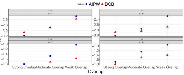
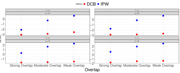
Figure 11: Comparison of DCB with AIPW and IPW (with estimated propensity score and estimated conditional mean function) over 200 replications. Low dimensional scenarios with $p\in\{10,20\}$. The y-axis report the MSE in log-scale the the x-axis reports different scenarios in terms of overlap (strong, moderate and weak overlap).

D.3 Comparisons as signal strength varies

In this section, we present simulations results with the same design as in Section 6 for a sparse setting ($p=10$), but with one distinction: we multiply the signal of the coefficients by $\eta\in\{0.1,0.3,0.5\}$ (overlap constant), varying the strength of the signal in the linear regression. This approach follows in spirit with simulations in Section 3 in Wüthrich and Zhu (2023). Similarly to what observed in Wüthrich and Zhu (2023), as the signal decreases ($\eta$ moves from $0.5$ to $0.1$ in our case), the performance of AIPW that uses lasso deteriorates. The relative improvements of DCB over AIPW increase as the signal strength decreases, further motivating the proposed method.

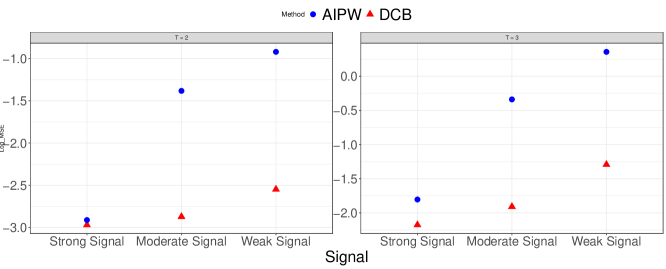
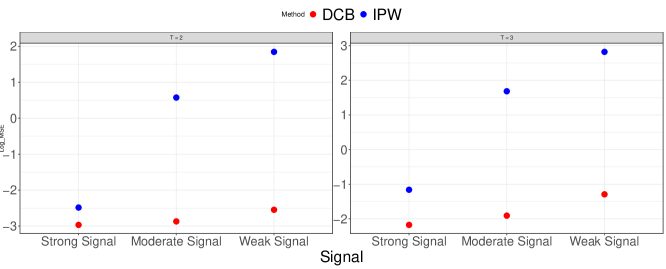
Figure 12: $p=100$, simulation design as in Section D with one difference: the coefficients $\beta$ multiply by $\eta$ with $\eta\in\{0.1,0.3,0.5\}$ (strong, moderate and weak signal, respectively). y-axis reports the MSE in log-scale.

Appendix E Effect of government contracts on local multipliers

In this section we offer a different application studying the effect of defense procurament contracts on local multipliers, using data from Auerbach et al. (2020). The finding in this application are consistent with the findings in our application in the main text.

A growing literature at the intersection of micro and macroeconomics focuses on estimating the effect of “local” fiscal multipliers, i.e., the effects of differential fiscal shocks at lower levels of aggregation within States in the United States. Examples include Auerbach et al. (2020); Nakamura and Steinsson (2014); Chodorow-Reich (2019) among others. A common method is to use variants of local projections (Jordà, 2005) to estimate short and long-term treatment effects. In this section, we illustrate how our procedure complements current practice using data from Auerbach et al. (2020).

E.1 Data and estimation

We follow Auerbach et al. (2020) and use change in defense government expenditure to construct the treatment of interest, available until 2016. The outcomes of interest are employment and growth rate, both available for 383 metropolitan areas. We augment the dataset in Auerbach et al. (2020) using census data at the metropolitan in the years 2010 - 2016 to control for many covariates. We construct four binary treatments: whether defense government spending has increased by at least $10,20,30\%$ over the previous year.

Figure LABEL:fig:treatment_path illustrates the dynamics of treatments for defense government spending exceeding at least $5\%$ the spending in the previous year. Most of the units switch treatment over time. Change in treatment may be associated with past growth rate, employment rate, level of government spending, and other factors, motivating controlling for many characteristics.

Our estimand of interest is formally defined as

$$\tau_{s}=\frac{1}{T}\sum_{t}\mathbb{E}\Big{[}Y_{i,t}(\mathbf{1}_{s},D_{i,(t-s):(-\infty)})-Y_{i,t}(\mathbf{0}_{s},D_{i,(t-s):(-\infty)})\Big{]},\quad s\in\{1,2,3\},$$ (49)

as the effect of being under treatment for one, two, or three most recent periods.

We consider a pooled estimation strategy over the years 2010 - 2016. We control for past growth rate, past employment rate, log defense government expenditure in the past two years, log population, migration rate, age distribution, and household size distribution, and in addition to those, we include state and time-fixed effects. Coefficients are estimated with a penalized linear regression (Algorithm 1 with model $=$ linear).

E.2 Results

Figure 13 reports treatment effects estimates of the proposed method (denoted as “$10,20,30\%$ DCB” in the figure’s legend). Each point $s$ on the x-axis corresponds to the average effect $\tau_{s}$. $90\%$-confidence intervals are depicted in gray. The darker gray area denotes confidence intervals with Gaussian quantiles, and the shaded gray area confidence intervals with (conservative) $\sqrt{\chi_{2T}}$-quantiles. Treatment effects are positive and increasing as we increase government spending from $10\%$ to $30\%$. Effects are also increasing as the number of periods of exposure to treatment increases from one to three years.

To illustrate the difference of our procedure from standard projection methods, Table 11 compares point estimates of our procedure with local projections for a $30\%$ increase in defense government spending. The standard local projection is estimated by projecting the observed outcome $Y_{t+2}$ onto the treatment $D_{t}$, controlling for time and unit fixed effects, as in Auerbach et al. (2020), and in the spirit of two-way fixed effect models.

The magnitude and sign of treatment effects estimated using our approach are comparable to the ones estimated via local projections by Auerbach et al. (2020). However, point estimates of the estimated (standard) local projection are smaller than estimates obtained with our approach at the three years horizon and comparable otherwise. Smaller point estimates at a longer horizon are intuitive: the standard local projection estimates the impulse response function, i.e., the effect of changing treatment in the previous three years, averaging over future (realized) treatment assignments. Here, we recover the different estimand $\tau_{s}$ that studies treatment effects for three consecutive periods.

Finally, for longer (three periods) horizons, the proposed approach presents a much smaller variance than the IPW estimator, with probabilities estimated via logistic regression. This result is intuitive as IPW is prone to poor overlap (larger variance) with a longer time horizon because probability weights depend on the joint probability of treatment history. We also compare balancing with the AIPW method that uses the same estimation strategy of DCB and balance covariates via inverse probability weights with such weights estimated using a high-dimensional (penalized) generalized linear model (Negahban et al., 2012). Here, DCB and AIPW present comparable results for employment, whereas we see a variance reduction by more than $50\%$ for estimating GDP at the three years horizon when using DCB.

Table 11: Effect of increasing defense government spending by $30\%$ over one, two or three periods ($s\in\{1,2,3\}$). DCB denotes the proposed method, AIPW uses the same outcome model as DCB and estimates the propensity score via a penalized logistic regression, IPW estimates inverse probability weights via a simple logistic regression and LP denotes a standard local projection of $Y_{i,t}$ on the treatment at time $t-s$, controlling for time and unit fixed effects.

	GDP				Emp
	DCB	AIPW	IPW	LP	DCB	AIPW	IPW	LP
$s=1$	0.29	0.20	0.36	0.30	0.14	0.14	0.10	0.06
	(0.33)	(0.25)	(0.31)	(0.12)	(0.12)	(0.10)	(0.18)	(0.12)
$s=2$	0.04	0.16	0.12	0.08	0.33	0.26	0.16	0.11
	(0.47)	(0.55)	(0.74)	(0.18)	(0.20)	(0.18)	(0.29)	(0.18)
$s=3$	1.04	2.19	2.63	0.11	0.49	0.69	1.09	0.09
	(1.09)	(1.75)	(2.36)	(0.17)	(0.55)	(0.47)	(1.24)	(0.17)

Figure 13: Effect of government spending: pooled regression from $t\in\{2010,\cdots,2016\}$ Gray region denotes the $90\%$ confidence band for treatments corresponding to a $30\%$ increase in defense government spending. The light-gray corresponding to the $\sqrt{\chi_{2T}(\alpha)}$ critical quantile, and darker area to the Gaussian critical quantile. $10,20,30\%$ denote correspond to different treatments as increasing defense government spending by $10,20,30\%$.

References

- Abbring and Van den Berg (2003) Abbring, J. H. and G. J. Van den Berg (2003). The nonparametric identification of treatment effects in duration models. Econometrica 71(5), 1491–1517.
- Abraham and Sun (2018) Abraham, S. and L. Sun (2018). Estimating dynamic treatment effects in event studies with heterogeneous treatment effects. Available at SSRN 3158747.
- Acemoglu et al. (2019) Acemoglu, D., S. Naidu, P. Restrepo, and J. A. Robinson (2019). Democracy does cause growth. Journal of Political Economy 127(1), 47–100.
- Alloza et al. (2020) Alloza, M., J. Gonzalo, and C. Sanz (2020). Dynamic effects of persistent shocks. arXiv preprint arXiv:2006.14047.
- Arkhangelsky and Imbens (2019) Arkhangelsky, D. and G. Imbens (2019). Double-robust identification for causal paneldata models. arXiv preprint arXiv:1909.09412.
- Athey and Imbens (2022) Athey, S. and G. W. Imbens (2022). Design-based analysis in difference-in-differences settings with staggered adoption. Journal of Econometrics 226(1), 62–79.
- Athey et al. (2018) Athey, S., G. W. Imbens, and S. Wager (2018). Approximate residual balancing: debiased inference of average treatment effects in high dimensions. Journal of the Royal Statistical Society: Series B (Statistical Methodology) 80(4), 597–623.
- Athey and Wager (2021) Athey, S. and S. Wager (2021). Policy learning with observational data. Econometrica 89(1), 133–161.
- Auerbach et al. (2020) Auerbach, A., Y. Gorodnichenko, and D. Murphy (2020). Local fiscal multipliers and fiscal spillovers in the usa. IMF Economic Review 68, 195–229.
- Babino et al. (2019) Babino, L., A. Rotnitzky, and J. Robins (2019). Multiple robust estimation of marginal structural mean models for unconstrained outcomes. Biometrics 75(1), 90–99.
- Bang and Robins (2005) Bang, H. and J. M. Robins (2005). Doubly robust estimation in missing data and causal inference models. Biometrics 61(4), 962–973.
- Belloni et al. (2014) Belloni, A., V. Chernozhukov, and C. Hansen (2014). Inference on treatment effects after selection among high-dimensional controls. The Review of Economic Studies 81(2), 608–650.
- Belloni et al. (2016) Belloni, A., V. Chernozhukov, C. Hansen, and D. Kozbur (2016). Inference in high-dimensional panel models with an application to gun control. Journal of Business & Economic Statistics 34(4), 590–605.
- Ben-Michael et al. (2018) Ben-Michael, E., A. Feller, and J. Rothstein (2018). The augmented synthetic control method. arXiv preprint arXiv:1811.04170.
- Blackwell (2013) Blackwell, M. (2013). A framework for dynamic causal inference in political science. American Journal of Political Science 57(2), 504–520.
- Bodory et al. (2020) Bodory, H., M. Huber, and L. Lafférs (2020). Evaluating (weighted) dynamic treatment effects by double machine learning. arXiv preprint arXiv:2012.00370.
- Bojinov et al. (2020) Bojinov, I., A. Rambachan, and N. Shephard (2020). Panel experiments and dynamic causal effects: A finite population perspective. arXiv preprint arXiv:2003.09915.
- Bojinov and Shephard (2019) Bojinov, I. and N. Shephard (2019). Time series experiments and causal estimands: exact randomization tests and trading. Journal of the American Statistical Association, 1–36.
- Boruvka et al. (2018) Boruvka, A., D. Almirall, K. Witkiewitz, and S. A. Murphy (2018). Assessing time-varying causal effect moderation in mobile health. Journal of the American Statistical Association 113(523), 1112–1121.
- Bradic et al. (2021) Bradic, J., W. Ji, and Y. Zhang (2021). High-dimensional inference for dynamic treatment effects. arXiv preprint arXiv:2110.04924.
- Bruns-Smith et al. (2023) Bruns-Smith, D., O. Dukes, A. Feller, and E. L. Ogburn (2023). Augmented balancing weights as linear regression. arXiv preprint arXiv:2304.14545.
- Bühlmann and Van De Geer (2011) Bühlmann, P. and S. Van De Geer (2011). Statistics for high-dimensional data: methods, theory and applications. Springer Science & Business Media.
- Caetano et al. (2022) Caetano, C., B. Callaway, S. Payne, and H. S. Rodrigues (2022). Difference in differences with time-varying covariates. arXiv preprint arXiv:2202.02903.
- Callaway and Sant’Anna (2019) Callaway, B. and P. H. Sant’Anna (2019). Difference-in-differences with multiple time periods. Available at SSRN 3148250.
- Chernozhukov et al. (2017) Chernozhukov, V., M. Goldman, V. Semenova, and M. Taddy (2017). Orthogonal machine learning for demand estimation: High dimensional causal inference in dynamic panels. arXiv preprint arXiv:1712.09988.
- Chernozhukov et al. (2018) Chernozhukov, V., C. Hansen, Y. Liao, and Y. Zhu (2018). Inference for heterogeneous effects using low-rank estimations. arXiv preprint arXiv:1812.08089.
- Chernozhukov et al. (2022) Chernozhukov, V., W. Newey, R. Singh, and V. Syrgkanis (2022). Automatic debiased machine learning for dynamic treatment effects and general nested functionals. arXiv preprint arXiv:2203.13887.
- Chodorow-Reich (2019) Chodorow-Reich, G. (2019). Geographic cross-sectional fiscal spending multipliers: What have we learned? American Economic Journal: Economic Policy 11(2), 1–34.
- de Chaisemartin and d’Haultfoeuille (2019) de Chaisemartin, C. and X. d’Haultfoeuille (2019). Two-way fixed effects estimators with heterogeneous treatment effects. Technical report, National Bureau of Economic Research.
- De Chaisemartin and d’Haultfoeuille (2022) De Chaisemartin, C. and X. d’Haultfoeuille (2022). Difference-in-differences estimators of intertemporal treatment effects. Technical report, National Bureau of Economic Research.
- Ding and Li (2019) Ding, P. and F. Li (2019). A bracketing relationship between difference-in-differences and lagged-dependent-variable adjustment. Political Analysis 27(4), 605–615.
- Dube et al. (2023) Dube, A., D. Girardi, O. Jorda, and A. M. Taylor (2023). A local projections approach to difference-in-differences event studies. Technical report, National Bureau of Economic Research.
- Farrell (2015) Farrell, M. H. (2015). Robust inference on average treatment effects with possibly more covariates than observations. Journal of Econometrics 189(1), 1–23.
- Ghanem et al. (2022) Ghanem, D., P. H. Sant’Anna, and K. Wüthrich (2022). Selection and parallel trends. arXiv preprint arXiv:2203.09001.
- Goodman-Bacon (2021) Goodman-Bacon, A. (2021). Difference-in-differences with variation in treatment timing. Journal of Econometrics.
- Hainmueller (2012) Hainmueller, J. (2012). Entropy balancing for causal effects: A multivariate reweighting method to produce balanced samples in observational studies. Political Analysis 20(1), 25–46.
- Hastie et al. (2015) Hastie, T., R. Tibshirani, and M. Wainwright (2015). Statistical learning with sparsity: the lasso and generalizations. CRC press.
- Heckman et al. (2016) Heckman, J. J., J. E. Humphries, and G. Veramendi (2016). Dynamic treatment effects. Journal of econometrics 191(2), 276–292.
- Heckman and Navarro (2007) Heckman, J. J. and S. Navarro (2007). Dynamic discrete choice and dynamic treatment effects. Journal of Econometrics 136(2), 341–396.
- Hernán et al. (2001) Hernán, M. A., B. Brumback, and J. M. Robins (2001). Marginal structural models to estimate the joint causal effect of nonrandomized treatments. Journal of the American Statistical Association 96(454), 440–448.
- Hirshberg and Wager (2017) Hirshberg, D. A. and S. Wager (2017). Augmented minimax linear estimation. arXiv preprint arXiv:1712.00038.
- Imai and Kim (2016) Imai, K. and I. S. Kim (2016). When should we use linear fixed effects regression models for causal inference with longitudinal data? Unpublished working paper. Retrieved September 19.
- Imai et al. (2018) Imai, K., I. S. Kim, and E. Wang (2018). Matching methods for causal inference with time-series cross-section data.
- Imai and Ratkovic (2014) Imai, K. and M. Ratkovic (2014). Covariate balancing propensity score. Journal of the Royal Statistical Society: Series B (Statistical Methodology) 76(1), 243–263.
- Imai and Ratkovic (2015) Imai, K. and M. Ratkovic (2015). Robust estimation of inverse probability weights for marginal structural models. Journal of the American Statistical Association 110(511), 1013–1023.
- Imbens (2000) Imbens, G. W. (2000). The role of the propensity score in estimating dose-response functions. Biometrika 87(3), 706–710.
- Imbens and Rubin (2015) Imbens, G. W. and D. B. Rubin (2015). Causal inference in statistics, social, and biomedical sciences. Cambridge University Press.
- Jiang and Li (2015) Jiang, N. and L. Li (2015). Doubly robust off-policy value evaluation for reinforcement learning. arXiv preprint arXiv:1511.03722.
- Jordà (2005) Jordà, Ò. (2005). Estimation and inference of impulse responses by local projections. American economic review 95(1), 161–182.
- Kallus and Santacatterina (2018) Kallus, N. and M. Santacatterina (2018). Optimal balancing of time-dependent confounders for marginal structural models. arXiv preprint arXiv:1806.01083.
- Kock and Tang (2015) Kock, A. B. and H. Tang (2015). Inference in high-dimensional dynamic panel data models. arXiv preprint arXiv:1501.00478.
- Krampe et al. (2020) Krampe, J., E. Paparoditis, and C. Trenkler (2020). Impulse response analysis for sparse high-dimensional time series. arXiv preprint arXiv:2007.15535.
- Lewis and Syrgkanis (2020) Lewis, G. and V. Syrgkanis (2020). Double/debiased machine learning for dynamic treatment effects via g-estimation. arXiv preprint arXiv:2002.07285.
- Li et al. (2018) Li, F., K. L. Morgan, and A. M. Zaslavsky (2018). Balancing covariates via propensity score weighting. Journal of the American Statistical Association 113(521), 390–400.
- Marx et al. (2022) Marx, P., E. Tamer, and X. Tang (2022). Parallel trends and dynamic choices. arXiv preprint arXiv:2207.06564.
- Montiel Olea and Plagborg-Møller (2021) Montiel Olea, J. L. and M. Plagborg-Møller (2021). Local projection inference is simpler and more robust than you think. Econometrica 89(4), 1789–1823.
- Nakamura and Steinsson (2014) Nakamura, E. and J. Steinsson (2014). Fiscal stimulus in a monetary union: Evidence from us regions. American Economic Review 104(3), 753–792.
- Negahban et al. (2012) Negahban, S. N., P. Ravikumar, M. J. Wainwright, B. Yu, et al. (2012). A unified framework for high-dimensional analysis of -estimators with decomposable regularizers. Statistical science 27(4), 538–557.
- Nie et al. (2021) Nie, X., E. Brunskill, and S. Wager (2021). Learning when-to-treat policies. Journal of the American Statistical Association 116(533), 392–409.
- Plagborg-Møller (2019) Plagborg-Møller, M. (2019). Bayesian inference on structural impulse response functions. Quantitative Economics 10(1), 145–184.
- Rambachan and Roth (2023) Rambachan, A. and J. Roth (2023). A more credible approach to parallel trends. Review of Economic Studies, rdad018.
- Rambachan and Shephard (2019) Rambachan, A. and N. Shephard (2019). A nonparametric dynamic causal model for macroeconometrics. Available at SSRN 3345325.
- Robins (1986) Robins, J. (1986). A new approach to causal inference in mortality studies with a sustained exposure period—application to control of the healthy worker survivor effect. Mathematical modelling 7(9-12), 1393–1512.
- Robins et al. (2000) Robins, J. M., M. A. Hernan, and B. Brumback (2000). Marginal structural models and causal inference in epidemiology.
- Roth (2022) Roth, J. (2022). Pretest with caution: Event-study estimates after testing for parallel trends. American Economic Review: Insights 4(3), 305–322.
- Roth et al. (2023) Roth, J., P. H. Sant’Anna, A. Bilinski, and J. Poe (2023). What’s trending in difference-in-differences? a synthesis of the recent econometrics literature. Journal of Econometrics.
- Rust (1994) Rust, J. (1994). Structural estimation of markov decision processes. Handbook of econometrics 4, 3081–3143.
- Shi et al. (2018) Shi, C., A. Fan, R. Song, and W. Lu (2018). High-dimensional a-learning for optimal dynamic treatment regimes. Annals of statistics 46(3), 925–957.
- Stock and Watson (2018) Stock, J. H. and M. W. Watson (2018). Identification and estimation of dynamic causal effects in macroeconomics using external instruments. The Economic Journal 128(610), 917–948.
- Tchetgen and Shpitser (2012) Tchetgen, E. J. T. and I. Shpitser (2012). Semiparametric theory for causal mediation analysis: efficiency bounds, multiple robustness, and sensitivity analysis. Annals of statistics 40(3), 1816.
- Tran et al. (2019) Tran, L., C. Yiannoutsos, K. Wools-Kaloustian, A. Siika, M. Van Der Laan, and M. Petersen (2019). Double robust efficient estimators of longitudinal treatment effects: Comparative performance in simulations and a case study. The international journal of biostatistics 15(2).
- Vansteelandt et al. (2014) Vansteelandt, S., M. Joffe, et al. (2014). Structural nested models and g-estimation: the partially realized promise. Statistical Science 29(4), 707–731.
- Wainwright (2019) Wainwright, M. J. (2019). High-dimensional statistics: A non-asymptotic viewpoint, Volume 48. Cambridge University Press.
- Wolf and McKay (2022) Wolf, C. K. and A. McKay (2022). What can time-series regressions tell us about policy counterfactuals? Technical report, National Bureau of Economic Research.
- Wüthrich and Zhu (2023) Wüthrich, K. and Y. Zhu (2023). Omitted variable bias of lasso-based inference methods: A finite sample analysis. The review of economics and statistics 105(4), 982–997.
- Yiu and Su (2018) Yiu, S. and L. Su (2018). Covariate association eliminating weights: a unified weighting framework for causal effect estimation. Biometrika 105(3), 709–722.
- Yiu and Su (2020) Yiu, S. and L. Su (2020). Joint calibrated estimation of inverse probability of treatment and censoring weights for marginal structural models. Biometrics.
- Zhang et al. (2013) Zhang, B., A. A. Tsiatis, E. B. Laber, and M. Davidian (2013). Robust estimation of optimal dynamic treatment regimes for sequential treatment decisions. Biometrika 100(3), 681–694.
- Zhou and Wodtke (2018) Zhou, X. and G. T. Wodtke (2018). Residual balancing weights for marginal structural models: with application to analyses of time-varying treatments and causal mediation. arXiv preprint arXiv:1807.10869.
- Zhu (2017) Zhu, Y. (2017). High-dimensional panel data with time heterogeneity: estimation and inference. Available at SSRN 2665374.
- Zubizarreta (2015) Zubizarreta, J. R. (2015). Stable weights that balance covariates for estimation with incomplete outcome data. Journal of the American Statistical Association 110(511), 910–922.