Empirical Bayes Model Averaging
with Influential Observations:
Tuning Zellner’s $g$ Prior for Predictive Robustness

Christopher M. Hans^a,∗, Mario Peruggia^a and Junyan Wang^a

^aDepartment of Statistics, The Ohio State University, Columbus, OH 43210, USA

* Corresponding author: (hans@stat.osu.edu)

Abstract

The behavior of Bayesian model averaging (BMA) for the normal linear regression model in the presence of influential observations that contribute to model misfit is investigated. Remedies to attenuate the potential negative impacts of such observations on inference and prediction are proposed. The methodology is motivated by the view that well-behaved residuals and good predictive performance often go hand-in-hand. Focus is placed on regression models that use variants on Zellner’s $g$ prior. Studying the impact of various forms of model misfit on BMA predictions in simple situations points to prescriptive guidelines for “tuning” Zellner’s $g$ prior to obtain optimal predictions. The tuning of the prior distribution is obtained by considering theoretical properties that should be enjoyed by the optimal fits of the various models in the BMA ensemble. The methodology can be thought of as an “empirical Bayes” approach to modeling, as the data help to inform the specification of the prior in an attempt to attenuate the negative impact of influential cases.

KEY WORDS: Bayesian regression; BMA; Outliers; Regression diagnostics; Residuals; Shrinkage estimation.

1 Introduction

While there are many strategies for Bayesian regression modeling when there is uncertainty about model composition, Bayesian model averaging has been predominant in both literature and practice over the last two decades. This is particularly true when prediction is the primary objective. In this setting, a prior distribution is first placed over the collection of all models under consideration. For each model $\mathcal{M}_{\gamma}$, a prior distribution is then placed on the model-specific parameters, leading to a joint posterior distribution over both models and parameters. Predictions of a new outcome $\tilde{\bm{Y}}$ are typically made by computing a weighted average of the predictions under all possible models,

$$\mbox{Pred}(\tilde{\bm{Y}})=\sum_{\gamma\in\Gamma}\mbox{Pred}(\tilde{\bm{Y}}\mid\mathcal{M}_{\gamma})w(\mathcal{M}_{\gamma}),$$

where $\Gamma$ is a set that indexes all models under consideration, $\mathcal{M}_{\gamma}$ is a particular model and $w(\mathcal{M}_{\gamma})$ is the weight assigned to model $\mathcal{M}_{\gamma}$ in the averaging. Most commonly, $\mbox{Pred}(\tilde{\bm{Y}})$ is taken to be $E(\tilde{\bm{Y}}\mid\bm{Y})$, which minimizes expected posterior predictive $L_{2}$ loss, in which case the model-specific predictions are $E(\tilde{\bm{Y}}\mid\bm{Y},\mathcal{M}_{\gamma})$ and the model-specific weights are the posterior probabilities $\pi(\mathcal{M}_{\gamma}\mid\bm{Y})$ (Bernardo and Smith, 1994). Reviews of BMA are provided in Hoeting et al. (1999) and Clyde and George (2004). The term “BMA” is quite general and can be applied to many different data-analytic settings. In this work, “BMA” refers to Bayesian model averaging for linear regression, where an analyst has available $p$ potential covariates and would like to average over the $2^{p}$ possible regression models that can be constructed using subsets of the covariates. Seminal work on regression model composition uncertainty, which underlies BMA, can be found in Mitchell and Beauchamp (1988), George and McCulloch (1993), Smith and Kohn (1996), George and McCulloch (1997), Raftery et al. (1997) and Chipman et al. (2001).

While methods for diagnosing and remedying model misfit are well-established and routinely taught in regression modeling courses (see, e.g., Neter et al., 1996; Cook and Weisberg, 1982), the literature on model misfit for Bayesian analyses of classical linear regression models is somewhat less well-developed. Addressing potential or known model misfit is sometimes accomplished by modifying the likelihood, writing down a model that is flexible enough to describe the observed data. One example is the use of heavy-tailed error distributions to accommodate outliers (West, 1984). Model-based approaches to outlier detection and residual analysis have been considered by Chaloner and Brant (1988) and Hoeting et al. (1996).

The corpus of literature on Bayesian regression modeling and, in particular, Bayesian averaging of many regression models has expanded greatly since the development of early work addressing model misfit in Bayesian regression. While existing work provides useful guidelines for thinking about model misfit for specific Bayesian models, it is not clear that it provides prescriptive guidelines that can be applied in many of the currently-used Bayesian regression modeling settings.

For example, priors related to Zellner’s $g$ prior (Zellner, 1986) have become one of the “standard” setups for Bayesian regression modeling. The popularity of such priors is due, in part, to their computational simplicity. Use of these priors requires choosing an approach for handling hyperparameters, which we refer to generically as $g$. Current popular approaches for handling $g$ include empirical Bayes (EB) methods that focus on specifying $g$ by maximizing the marginal likelihood of the data with respect to either a single model or a mixture of models. Fully Bayes approaches assign a prior distribution to $g$ and then integrate it out of the model. While these approaches are sound when the model fits well, it is less clear that maximizing the marginal likelihood or integrating $g$ out of the model will be optimal in the presence of model misfit due to influential outliers, as the discrepancy between prior and likelihood may result in sub-optimal out-of-sample inference (say, the prediction of new cases).

In this work, we focus on methods of model specification in the presence of influential outliers that are strongly connected to the concept of residual analysis. We take the view that well-behaved residuals and good predictive performance usually go hand-in-hand. Any particular choice for handling $g$ corresponds to a specific Bayesian model and hence specific fitted values and residuals. By tuning the value of $g$ in Zellner’s $g$ prior over a continuous interval, we obtain continuously-varying residuals. Broadly speaking, in the presence of model misfit we seek to choose a value of $g$ that yields well-behaved residuals and hence attenuates the impact of the model misfit and, ultimately, achieves better out-of-sample predictive performance. In practice, we seek to find prescriptive guidelines for accomplishing this task by focusing on minimizing prediction error. Our investigation concerns not only an individual regression model but also an entire ensemble of regression models that may be combined together via BMA. In this case, model misfit due to influential outliers can exist at both the local (individual model) level and the global (model-averaged) level. By tuning the priors to attenuate the impact of model misfit, we eventually achieve improved out-of-sample predictive performance.

In Section 2 we introduce our regression model setting and review Zellner’s $g$ prior. Section 3 makes connections between the choice of $g$ and optimal prediction in the presence of influential outliers, and provides prescriptive guidelines for tuning Zellner’s $g$ prior. Section 4 describes the approach we have developed for applying these prescriptive guidelines in practice, and Section 5 investigates the performance of this approach in simulation studies. Section 6 applies our approach in an analysis of a data set and compares its predictive performance to other common methods. A summary of the results and a discussion of open questions and related work are provided in Section 7.

2 Regression model setting

We consider situations where an analyst observes an $n\times 1$ vector of response values, $\bm{Y}$, and an $n\times p$ matrix $\bm{X}$ which contains $p$ covariate values for each of the $n$ cases. As is common in the literature, unless specified otherwise, we assume throughout that the columns of $\bm{X}$ have been mean centered (see, e.g., Liang et al., 2008; Bayarri et al., 2012; Li and Clyde, 2018, for justifications and discussion of this modeling choice). There are $2^{p}$ possible subsets of the $p$ covariates that could be used to construct a mean function for a linear regression model, and interest lies in computing model-averaged predictions as described in Section 1 over the space of all possible regression models. In this setup, a model $\mathcal{M}_{\gamma}$ corresponds to a subset of $k$ predictors. We use the binary $p$-vector $\gamma$ to index all possible models: $\gamma_{j}=1$ when $X_{j}$ is included in a model and $\gamma_{j}=0$ otherwise. The notation $\mathcal{M}_{\gamma}$ is used to denote a model containing predictors indicated by the vector $\gamma$. Other quantities subscripted by $\gamma$ denote model-specific terms, e.g. $\bm{X}_{\gamma}$ is the $n\times k$ matrix which contains the columns of $\bm{X}$ that are included in model $\mathcal{M}_{\gamma}$.

Our work focuses on data analysis settings where either (i) the total number of predictors $p$ is not too large or (ii) where $p$ may be large, but we constrain the maximum number of predictors in a model to be $k^{*}\ll p$ (e.g., as in Hans et al., 2007). The simulations and examples presented in Sections 5 and 6 consider $p$ as large as ten. We focus on small-$p$ settings in part because they are relevant for a wide swath of applied data analysis, where an investigator is interested in understanding the relationship between a small set of regressors and a response variable, and in part due to the computational challenges associated with averaging over very large model spaces that are faced by all BMA methods.

BMA requires hierarchical specification of a prior probability, $\pi(\mathcal{M}_{\gamma})$, for each model under consideration, and then, for each model, a likelihood and a prior for the model-specific regression parameters. For normal linear regression modeling, the likelihood for a specific model $\mathcal{M}_{\gamma}$ is derived from the distribution of $\bm{Y}$ given the model parameters, $(\alpha,\bm{\beta}_{\gamma},\sigma^{2})$,

$$p(\bm{Y}\mid\alpha,\bm{\beta}_{\gamma},\sigma^{2},\mathcal{M}_{\gamma})=\mbox{N}(\bm{Y}\mid\alpha\mathbf{1}_{n}+\bm{X}_{\gamma}\bm{\beta}_{\gamma},\sigma^{2}I_{n}),$$

where $\bm{\beta}_{\gamma}$ are the regression coefficients corresponding to the predictors $\bm{X}_{\gamma}$ in model $\mathcal{M}_{\gamma}$, $\alpha$ is an intercept, $\sigma^{2}$ is the error variance, $\mathbf{1}_{n}$ is an $n\times 1$ vector of ones, and $I_{n}$ is the $n\times n$ identity matrix. The model-specific priors on the parameters are known to play a key role in inference and prediction, and there are many possibilities for their specification. A common approach, which we adopt in this work, is to assume $\pi(\alpha,\bm{\beta}_{\gamma},\sigma^{2}\mid\mathcal{M}_{\gamma})=\pi(\bm{\beta}_{\gamma}\mid\sigma^{2},\mathcal{M}_{\gamma})\pi(\alpha,\sigma^{2}\mid\mathcal{M}_{\gamma})$ and to use the improper, “objective” prior $\pi(\alpha,\sigma^{2}\mid\mathcal{M}_{\gamma})\propto\sigma^{-2}$ (Jeffreys, 1961; Berger et al., 1998).

Various approaches to specifying the prior probabilities $\pi(\mathcal{M}_{\gamma})$ have been studied in the literature. While the uniform prior over models, $\pi(\mathcal{M}_{\gamma})=2^{-p}$, was discussed in the early Bayesian variable selection literature (George and McCulloch, 1993), it does not control the false positive rate in the context of variable selection when making multiple comparisons (Scott and Berger, 2010). An alternate prior formulation that provides better multiplicity control is the $\mbox{Beta-Binomial}(1,1)$ prior, $\pi(\mathcal{M}_{\gamma})=(p+1)^{-1}{p\choose|\mathcal{M}_{\gamma}|}^{-1}$, where $|\mathcal{M}_{\gamma}|$ is the number of variables in model $\mathcal{M}_{\gamma}$ (Ley and Steel, 2009; Scott and Berger, 2010). This is a special case of the Beta-Binomial prior considered by Kohn et al. (2001) and can be interpreted as first specifying a uniform prior over model size and then, conditionally on model size, specifying a uniform prior over models. More recent advances in model space prior specification include the loss-based prior of Villa and Lee (2020). Unless specified otherwise, we use the $\mbox{Beta-Binomial}(1,1)$ prior in this work.

The research literature on priors for the model-specific regression coefficients, $\pi(\bm{\beta}_{\gamma}\mid\sigma^{2},\mathcal{M}_{\gamma})$, is extensive. Historically, one of the most popular classes of priors for the regression coefficients is based on Zellner’s $g$ prior,

$$\bm{\beta}_{\gamma}\mid\sigma^{2},\mathcal{M}_{\gamma}\sim\mbox{N}(0,g_{\gamma}\sigma^{2}(\bm{X}_{\gamma}^{T}\bm{X}_{\gamma})^{-1}),$$ (1)

where $g_{\gamma}>0$ is a hyperparameter (Zellner, 1986). This prior has received much attention in the literature and in practice due in part to the fact that, for specific treatments of $g_{\gamma}$, Zellner’s $g$-prior allows for computationally efficient model averaging when $p$ is not too large. In the context of BMA, when minimizing expected posterior predictive $L_{2}$ loss, model averaged predictions require calculation of $E(\bm{\beta}_{\gamma}\mid\bm{Y},\mathcal{M}_{\gamma})$ and $\pi(\mathcal{M}_{\gamma}\mid\bm{Y})\propto m(\bm{Y}\mid\mathcal{M}_{\gamma})\pi(\mathcal{M}_{\gamma})$ for each model, where $m(\bm{Y}\mid\mathcal{M}_{\gamma})$ is the marginal likelihood for model $\mathcal{M}_{\gamma}$. Closed form expressions for these quantities exist when $g_{\gamma}$ is treated as a constant in the model. The marginal likelihood for model $\mathcal{M}_{\gamma}$ is

$$m(\bm{Y}\mid\mathcal{M}_{\gamma}) = \int p(\bm{Y}\mid\alpha,\bm{\beta}_{\gamma},\sigma^{2},\mathcal{M}_{\gamma})\pi(\alpha,\bm{\beta}_{\gamma},\sigma^{2}\mid\mathcal{M}_{\gamma})\,d\alpha\,d\bm{\beta}_{\gamma}\,d\sigma^{2}$$

$$= \frac{\Gamma((n-1)/2)}{\pi^{(n-1)/2}n^{1/2}|\!|\bm{Y}-\bar{\bm{Y}}|\!|^{n-1}}\frac{(1+g_{\gamma})^{(n-k-1)/2}}{(1+g_{\gamma}(1-R_{\gamma}^{2}))^{(n-1)/2}},$$

where $\bar{\bm{Y}}$ is the $n\times 1$ vector where all elements are equal to the sample average value of the $Y_{i}$’s, $|\!|\cdot|\!|$ is the $L_{2}$ norm and $R^{2}_{\gamma}$ is the coefficient of determination for model $\mathcal{M}_{\gamma}$. The posterior mean of the regression coefficients under model $\mathcal{M}_{\gamma}$ is

$$E(\bm{\beta}_{\gamma}\mid\bm{Y},\mathcal{M}_{\gamma})=\frac{g_{\gamma}}{1+g_{\gamma}}\hat{\bm{\beta}}_{LS},$$ (2)

where $\hat{\bm{\beta}}_{LS}$ is the ordinary least squares estimate of $\bm{\beta}_{\gamma}$ under model $\mathcal{M}_{\gamma}$, and $\rho_{\gamma}=g_{\gamma}/(1+g_{\gamma})\in(0,1)$ is sometimes called the shrinkage factor. Under this model, the prior combines with the data to shrink the least squares estimate toward zero by a factor of $\rho_{\gamma}$. Computation of all of these quantities is trivial once the usual calculations for least-squares estimation have been performed.

Specification (or modeling) of $g_{\gamma}$ is important, as it impacts the marginal likelihood, which in turn impacts model averaging. There is a large literature discussing methods for handling this parameter. Approaches that specify fixed values of the $g_{\gamma}$ include the unit information prior (Kass and Wasserman, 1995), the risk inflation criterion (Foster and George, 1994), the local empirical Bayes prior (Hansen and Yu, 2001) and the global empirical Bayes prior (George and Foster, 2000; Clyde and George, 2000). Some of these approaches specify a single $g$ that is common to all models, while others specify different $g_{\gamma}$’s for different models. Som et al. (2014) use different $g_{\gamma}$’s for different groups of predictor variables. Liang et al. (2008) and Bayarri et al. (2012) provide motivation for assigning a prior distribution to $g$ and suggest priors that enjoy appealing theoretical properties while maintaining computational tractability. Other priors for $g$ have been proposed by Zellner and Siow (1980), West (2003), Cui and George (2008), Maruyama and Strawderman (2010), and Maruyama and George (2011).

The method we describe in Section 4 can be viewed as an empirical Bayes approach to specifying hyperparameter values, and so existing empirical Bayes methods are of special interest to us. Global empirical Bayes methods use the data to estimate a hyperparameter $g$ that is common to all models. The parameter is typically estimated by maximizing the marginal likelihood of the observed data given $g$, $m(\bm{Y}\mid g)=\sum_{\gamma\in\Gamma}m(\bm{Y}\mid\mathcal{M}_{\gamma},g)\pi(\mathcal{M}_{\gamma})$, where the parameters $\alpha$, $\bm{\beta}_{\gamma}$ and $\sigma^{2}$ have been integrated out of each model to obtain the model-specific marginal likelihood $m(\bm{Y}\mid\mathcal{M}_{\gamma},g)$. Clyde (2001) describes an EM algorithm that can be used to find the value of $g$ that maximizes the model-averaged marginal likelihood. The local empirical Bayes approach allows for different $g_{\gamma}$ for each model and uses the data to estimate them by maximizing the model-specific marginal likelihood $m(\bm{Y}\mid\mathcal{M}_{\gamma},g_{\gamma})$. While empirical Bayes approaches use the data to estimate specific values $g_{\gamma}$, fully-Bayesian approaches assign prior distributions to the $g_{\gamma}$ and use the data to integrate over uncertainty about them a posteriori. Of the fully-Bayes methods, the hyper-$g/n$ prior of Liang et al. (2008) is noteworthy as it is amenable to efficient computation and has desirable theoretical properties. This approach assigns the prior $\pi(g_{\gamma}\mid\mathcal{M}_{\gamma})=(a-2)(1+g_{\gamma}/n)^{-1/2}/(2n)$, with $a=3$ recommended as a default specification. We compare our method to these three approaches in Section 5.

The prior mean vector $E(\bm{\beta}_{\gamma}\mid\sigma^{2},\mathcal{M}_{\gamma})$ is routinely taken to be the zero vector in (1). When lacking prior information about the location of the vector of regression coefficients, centering the prior at zero shrinks the posterior distribution toward zero—corresponding to no linear association between $\bm{Y}$ and the collection of predictors $\bm{X}_{\gamma}$—as can be seen in (2). Zellner’s original formulation of the $g$ prior (Zellner, 1986) allowed for shrinkage toward non-zero mean vectors. In this case, we write the prior as

$$\bm{\beta}_{\gamma}\mid\sigma^{2},\mathcal{M}_{\gamma}\sim\mbox{N}(\bm{\theta}_{\gamma},g_{\gamma}\sigma^{2}(\bm{X}_{\gamma}^{T}\bm{X}_{\gamma})^{-1}),$$ (3)

where $\bm{\theta}_{\gamma}$ is the prior mean vector for $\bm{\beta}_{\gamma}$. Under this prior, the posterior mean of $\bm{\beta}_{\gamma}$ under model $\mathcal{M}_{\gamma}$ is

$$E(\bm{\beta}_{\gamma}\mid\bm{Y},\mathcal{M}_{\gamma})=\frac{1}{1+g_{\gamma}}\bm{\theta}_{\gamma}+\frac{g_{\gamma}}{1+g_{\gamma}}\hat{\bm{\beta}}_{LS}=(1-\rho_{\gamma})\bm{\theta}_{\gamma}+\rho_{\gamma}\hat{\bm{\beta}}_{LS},$$

where $\rho_{\gamma}=g_{\gamma}/(1+g_{\gamma})$, called the shrinkage factor above, can now be interpreted as determining the posterior mean as a convex combination of the prior mean of $\bm{\beta}_{\gamma}$ and the data-based estimate of $\bm{\beta}_{\gamma}$. The marginal likelihood under prior (3) for a model $\mathcal{M}_{\gamma}$ with $k$ predictors is

$$m(\bm{Y}\mid\mathcal{M}_{\gamma}) = \frac{\Gamma((n-1)/2)}{\pi^{(n-1)/2}n^{1/2}}|\!|\bm{Y}-\bar{\bm{Y}}|\!|^{-(n-1)}(1+g_{\gamma})^{(n-k-1)/2}$$ (4)

$$\hskip 72.26999pt\times\left(1+g_{\gamma}(1-R_{\gamma}^{2})+\frac{|\!|\bm{Y}-\bm{X}_{\gamma}\bm{\theta}_{\gamma}|\!|^{2}-|\!|\bm{Y}|\!|^{2}}{|\!|\bm{Y}-\bar{\bm{Y}}|\!|^{2}}\right)^{-\frac{n-1}{2}}.$$

Dividing (4) by the marginal likelihood for the “null model”, $\mathcal{M}_{N}$—the model with no predictors that assumes a common mean for all $Y_{i}$—yields the Bayes factor for comparing model $\mathcal{M}_{\gamma}$ to model $\mathcal{M}_{N}$:

$$BF(\mathcal{M}_{\gamma}:\mathcal{M}_{N})=(1+g_{\gamma})^{(n-k-1)/2}\left(1+g_{\gamma}(1-R_{\gamma}^{2})+\frac{||\bm{Y}-\bm{X_{\gamma}\theta_{\gamma}}||^{2}-||\bm{Y}||^{2}}{||\bm{Y}-\bm{\bar{Y}}||^{2}}\right)^{-\frac{n-1}{2}}.$$ (5)

We revisit this version of Zellner’s $g$ prior in Section 4.1.

3 Outliers and Model-Averaged Prediction Accuracy

Model-averaged predictions for linear regression depend on the posterior distribution over models, $\pi(\mathcal{M}_{\gamma}\mid\bm{Y})$, and the within-model estimates of the regression coefficients, $E(\bm{\beta}_{\gamma}\mid\bm{Y},\mathcal{M}_{\gamma})$, both of which depend on $g_{\gamma}$. When $p$ predictors are available and we are averaging over the space $\Gamma$ of all possible $2^{p}$ models, the model-averaged predictions of $n$ new cases $\tilde{\bm{Y}}$ at the same matrix of regressors $\bm{X}$ used to fit the model can be written as

$$\mbox{Pred}(\tilde{\bm{Y}}) = \sum_{\gamma\in\Gamma}\mbox{Pred}(\tilde{\bm{Y}}\mid\mathcal{M}_{\gamma})\pi(\mathcal{M}_{\gamma}\mid y)$$

$$= \sum_{\gamma\in\Gamma}\left(\bar{\bm{Y}}+\bm{X}_{\gamma}E(\bm{\beta}_{\gamma}\mid\bm{Y},\mathcal{M}_{\gamma})\right)\pi(\mathcal{M}_{\gamma}\mid\bm{Y})$$

$$= \bar{\bm{Y}}+\bm{X}E(\bm{\beta}\mid\bm{Y}),$$

where, for $j=1,\ldots,p$, the $j$th element of the vector $E(\bm{\beta}\mid\bm{Y})$,

$$E(\beta_{j}\mid\bm{Y})=\sum_{\gamma\in\Gamma\;:\;X_{j}\in\mathcal{M}_{\gamma}}E(\beta_{\gamma,X_{j}}\mid\bm{Y},\mathcal{M}_{\gamma})\pi(\mathcal{M}_{\gamma}\mid\bm{Y}),$$

is the model-averaged estimate of $\beta_{j}$, and the sum is taken over all models that include $X_{j}$ as a regressor. The notation $\beta_{\gamma,X_{j}}$ is used to denote the coefficient in model $\mathcal{M}_{\gamma}$ that corresponds to regressor $X_{j}$. We denote the model-averaged estimate of the regression coefficients as $\hat{\bm{\beta}}_{BMA}\equiv E(\bm{\beta}\mid\bm{Y})$.

In this section, we present several examples to illustrate the impact of influential outliers on BMA. In particular we focus on the relationship between outlying value(s), the choice of $g_{\gamma}$ in the prior, and predictive accuracy. The examples shed light on the behavior of BMA in the presence of influential outliers and suggest general strategies for improving model-averaged prediction. Example 1 illustrates the sensitivity of the posterior distribution over models to outliers in an example with three potential predictors. Example 2 focuses on the impact of outliers on model-averaged prediction in a stylized example. This example makes connections between the behavior of residuals and optimal prediction. Sections 3.3 and 3.4 generalize these results to mean-shift and variance-inflation contamination settings with an arbitrary number of predictors, $p$. The examples and results in this section provide the intuition behind the prescriptive guidelines for selecting $g_{\gamma}$ that we pursue in Section 4.

3.1 Example 1: Impact of Outliers on the Posterior

We first present a simple example that illustrates the impact of a single contaminated case on the posterior distribution over models. Let $X_{i1}=i-1-(n-1)/2$, for $i=1,\ldots,n=11$, so that the $X_{i1}$ take the values $-5,-4,\ldots,4,5$ and are mean-centered with $\sum_{i=1}^{n}X_{i1}=0$. Suppose that the true regression line is given by $E(Y_{i}\mid X_{i})=\beta X_{i1}$ and that the data are generated according to

$$Y_{i}=\beta X_{i1}+I(i=j)K+\epsilon_{i},\,\,i=1,\ldots,n,$$

with $\epsilon_{i}\stackrel{{\scriptstyle iid}}{{\sim}}{\rm N}(0,1)$ and $\beta=0.5$, where $I(i=j)$ is a 0/1 indicator function that is nonzero only for case $j$. In this setup, $K\neq 0$ means the response for case $j$ is a contaminated value and constitutes an outlier if $|K|$ is large. Case $j$ will also have high leverage for small and large values of $j$. We simulated $(X_{i1},Y_{i})$ pairs with $n=11$, $\beta=0.5$ and $\sigma^{2}=1$. We also simulated (and then mean centered) two other potential predictor variables: $X_{i2}=X_{i1}+Z_{i}$, with $X_{i}\stackrel{{\scriptstyle iid}}{{\sim}}{\rm N}(0,1)$ so that $X_{1}$ and $X_{2}$ are highly correlated, and $X_{i3}\stackrel{{\scriptstyle iid}}{{\sim}}{\rm N}(0,1)$ with $X_{3}$ independent of $Y$, $X_{1}$ and $X_{2}$. Considering all three potential predictors, the model space contains $2^{3}=8$ possible models (including the null model, containing only an intercept), over which we place a prior distribution that is uniform over model size and, conditional on model size, uniform over models. For each of the non-null models, the prior distribution on the regression coefficients is taken to be Zellner’s $g$-prior centered at zero with $g=n$, corresponding to a unit information prior (Kass and Wasserman, 1995; Fernández et al., 2001). The prior is completed with the standard non-informative prior $\pi(\alpha,\sigma^{2})\propto\sigma^{-2}$.

For a given contaminated case location $j$, we are interested in the impact of $K$ on the posterior probabilities of the eight models. The top row of Figure 1 displays this impact as $K$ ranges from $-10$ to $10$ for $j=1$ (so that the contaminated case corresponds to the smallest $X_{1}$ value), $j=6$ (medium $X_{1}$ value) and $j=11$ (largest $X_{1}$ value). The binary vector $\gamma$ distinguishes the eight models: $(0,0,0)$ corresponds to the model that includes none of the three predictors, $(1,0,0)$ contains only $X_{1}$, $(0,1,1)$ contains $X_{2}$ and $X_{3}$, etc. Clearly, the posterior distribution is quite sensitive to the contaminated case. In cases where the contaminated case attenuates the relationship between $X_{1}$ and $Y$ ($j\approx 1$, $K\approx 10$; $j\approx 11$, $K\approx-10$), the null model becomes more heavily weighted than when there is no contaminated case. In other cases (e.g., $j=11$, $K\approx 10$), the posterior shifts toward models that include too many predictors. When $K=0$ there is no outlier, and so the posterior model probabilities will be the same in each plot ($j=1,6,11$) as indicated by the plotted points.

The marginal inclusion probabilities for each predictor $j$,

$$\pi(\gamma_{j}=1\mid\bm{Y})=\sum_{\gamma\in\Gamma\;:\;\gamma_{j}=1}\pi(\mathcal{M}_{\gamma}\mid\bm{Y}),$$

play an important role in assessing model uncertainty from a Bayesian perspective. Barbieri and Berger (2004) provide conditions under which the median probability model (MPM)—the model that includes all predictors with $\pi(\gamma_{j}=1\mid\bm{Y})\geq 0.5$—is Bayes-optimal for prediction when a single model is to be selected. Carvalho and Lawrence (2008) provide decision-theoretic support for reporting the MPM under a model selection framework. Marginal inclusion probabilities also play a key role in many computational approaches for BMA (e.g., Clyde et al., 2011).

The bottom row of Figure 1 displays how outlier location, magnitude and direction impact the marginal inclusion probabilities for each of the three predictors in this example. The probabilities are clearly sensitive to the nature of the outlier. When $K=0$ (no outlier), the MPM just barely selects the generative model ($X_{1}$ only); the marginal inclusion probability for $X_{2}$ is $0.4996$. Outlier contamination suppresses marginal inclusion probabilities in some cases (outlier location $j=1$, $K$ large; $j=6$, $|K|$ large) while amplifying them in others ($j=11$, $K$ large). Model-averaged inference and prediction depend on the posterior weights for the individual models, which we learn from this example can be impacted greatly by the presence of an influential outlier. This motivates the need to study the impact of outliers on BMA predictive accuracy, which we explore in the next example.

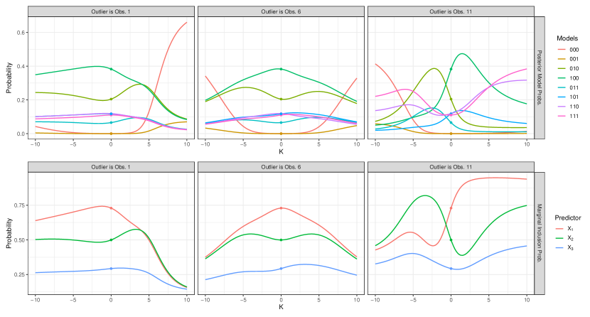
Figure 1: Posterior model probabilities (top row) and marginal inclusion probabilities (bottom row) for Example 1 in Section 3.1. Models in the top row are indexed by $\gamma$, e.g. “010” indicates the model with only $X_{2}$ as a predictor.

3.2 Example 2: Impact on Prediction

This example considers a simplified version of Example 1 in order to illustrate clearly how the choice of $g$ in the $g$ prior impacts model averaged prediction accuracy in the presence of an influential outlier. In this example we consider a single potential predictor $X$ and assume the true mean is given by $E(Y\mid X)=\beta X$. The observed values $X_{i}$, $i=1,\ldots,n=11$, are the same as the values of $X_{i1}$ in Example 1: $X_{i}=i-1-(n-1)/2$. Now, however, we assume that $Y_{i}$ is observed without error for $i=1,\ldots,n-1$, so that $Y_{i}=\beta X_{i}$, and we assume that $Y_{n}=\beta X_{n}-K$. In this example, the first $n-1$ training data points are observed without error because for now we are interested exclusively in quantifying the impact of the influential observation. After developing intuition in this stylized example, we consider the usual setting where data are observed with error in Sections 3.3 and 3.4 and in the rest of the work. The data are plotted in Figure 2 for three different value of $K$.

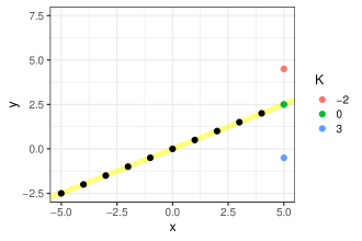
Figure 2: Simple linear regression data with contaminants for Example 3.2

There are two models under consideration: the null model $\mathcal{M}_{N}$ with only an intercept term, and the full model $\mathcal{M}_{1}$ that includes $X$ as a regressor. Letting $\bm{X}$ be the $n\times 1$ matrix of regressor values, under $L_{2}$ loss the Bayes estimators of the mean functions at $\bm{X}$ for these two models under Zellner’s $g$ prior (1) are

$$\hat{E}(\bm{Y}\mid\bm{X},\mathcal{M}_{N}) = \bar{\bm{Y}}=-\mathbf{1}_{n}\frac{K}{n},$$

$$\hat{E}(\bm{Y}\mid\bm{X},\mathcal{M}_{1}) = \bar{\bm{Y}}+\frac{g}{1+g}\bm{X}(\bm{X}^{T}\bm{X})^{-1}\bm{X}^{T}\bm{Y}$$

$$= -\mathbf{1}_{n}\frac{K}{n}+\frac{g}{1+g}\bm{X}\hat{\beta}_{LS}.$$

Suppose we observe testing data at $n$ design points $\tilde{X}_{i}$. We assume the $\tilde{Y}_{i}$ values in the testing data follow the true regression line, $E(\tilde{Y}_{i}\mid\tilde{X}_{i})=\beta\tilde{X}_{i}$, plus independent Gaussian error $\epsilon_{i}$ with mean zero and variance $\sigma^{2}$. Case $n$ in the test data set is assumed to be observed without contamination $(K=0)$. The $\mbox{Beta-Binomial}(1,1)$ prior over the model space assigns prior probabilities of $1/2$ to each model and leads to the model-averaged predictions

$$\hat{\bm{Y}}=\frac{g}{1+g}w(g,\bm{Y})\tilde{\bm{X}}\hat{\beta}_{LS}-\mathbf{1}_{n}\frac{K}{n},$$

where $w(g,\bm{Y})=\pi(\mathcal{M}_{1}\mid\bm{Y})$ is the weight (posterior probability) for model $\mathcal{M}_{1}$. We further define $s(g,\bm{Y})=(g/(1+g))w(g,\bm{Y})$ to be the shrinkage factor for the model-averaged estimate of $\beta$: the factor by which the least squares estimate of $\beta$ is shrunk toward zero when averaging over the two models. The shrinkage factor $s(g,\bm{Y})$ is a non-linear function of $g$.

With the model-averaged predictions in hand, we can quantify predictive accuracy by computing the expected mean squared prediction error over the distribution of the test data $\tilde{\bm{Y}}$ as a function of $g$, conditioned on the observed data $\bm{Y}$:

$$E(MSPE(g)\mid\bm{Y})=E\left[\frac{1}{n}\sum_{i=1}^{n}(\tilde{Y}_{i}-\hat{Y}_{i})^{2}\right]\\ =\frac{1}{n}\left[\left(\beta-s(g,\bm{Y})\hat{\beta}_{LS}\right)^{2}\left(\sum_{i=1}^{n}\tilde{X}_{i}^{2}\right)+2\,\frac{K}{n}\left(\beta-s(g,\bm{Y})\hat{\beta}_{LS}\right)\left(\sum_{i=1}^{n}\tilde{X}_{i}\right)\right]+\frac{K^{2}}{n^{2}}+\sigma^{2}.$$

The expected mean squared prediction error is therefore minimized, as a function of $g$, when

$$s(g,\bm{Y})\hat{\beta}_{LS}=\beta+\frac{\sum_{i=1}^{n}\tilde{X}_{i}(K/n)}{\sum_{i=1}^{n}\tilde{X}_{i}^{2}},$$ (6)

i.e., when the model-averaged prediction line is parallel to a line whose slope is the sum of two terms: the slope of the true regression line and the estimated least squares slope for a data set in which the observations taken at the $n$ design points $\tilde{X}_{i}$ are all equal to $K/n$.

The optimal value of $g$ is thus seen to depend on the the true model slope, the testing design points, and the size $K$ of the contamination. In a situation where the validation design points and the contamination size are random, one could make use of existing knowledge of certaing aspects of their distributions to obtain a plausible value for the second term in the RHS of Equation (6). For example, expected values for $\sum_{i=1}^{n}\tilde{X}_{i}$, $\sum_{i=1}^{n}\tilde{X}_{i}^{2},$ and $K$ could be substituted into the expression. Of special interest is the situation where the testing design points $\tilde{X}_{i}$ coincide with the design points in the training data set. If that happens, then $\sum_{i=1}^{n}\tilde{X}_{i}=0$ and the optimal value of $g$ is the one that makes the model-averaged prediction line parallel to the true regression line. We focus on this situation when developing our methods. The simulation examples in Section 5 examine the behavior of our method when the testing locations $\tilde{\bm{X}}$ are allowed to differ from the training locations $\bm{X}$.

Having characterized the $g$ that leads to optimal predictions, we examine as a function of $g$ the behavior of the quantities $w(g,\bm{Y})$, $s(g,\bm{Y})$, and $E(MSPE(g)\mid\bm{Y})$ when $n=11$, $\beta=0.5$, $K=-5$, and $\sigma^{2}=1$. These quantities are plotted in Figure 3. A question of interest is how the value of $g$ that minimizes expected mean squared prediction error described above compares to other choices of $g$, e.g., the local empirical Bayes estimate. For interpretability, it is helpful to work on the transformed scale $\rho=g/(1+g)$. The red diamond in the top panel of Figure 3 shows that the local empirical Bayes value of $\rho$, i.e., the value of $\rho$ that maximizes the posterior model weight, is given by $\rho=0.967$ (or $\log g=3.378$), yielding $w(g=e^{3.378},\bm{Y})=0.994$. The red diamond in the middle panel tracks the corresponding shrinkage $s(g=e^{3.378},\bm{Y})=0.962$, and the red diamond in the bottom panel tracks the corresponding expected mean squared prediction error, $E(MSPE(g=e^{3.378}\mid\bm{Y}))=1.604$.

The green diamond in the bottom panel, however, shows that the expected squared error of prediction is minimized for $\rho=0.711$ (or $\log g=0.901$) where $E(MSPE(g=e^{0.901}\mid\bm{Y}))=1.207$. The corresponding values of the model weight and shrinkage, tracked by the green diamonds in the top and middle panel, are $0.967$ and $0.688$. The optimal value of $\rho$ is much smaller than the one suggested by local empirical Bayes and much more shrinkage is needed to minimize the expected MSPE.

Figure 3 shows that additional interesting features occur for values of $\rho$ approaching 1 from the left ($g$ going to infinity). For one thing, as a consequence of Bartlett’s paradox (Liang et al., 2008), the posterior weight assigned to the regression model goes to zero and the null model gets fully weighted. Equation (3.2) says that setting $\rho=0$ ($g=0$) and $\rho=1$ ($g=\infty$) will yield the same predictions. Hence, the expected MSPE is the same at $\rho=0$ and $\rho=1$. As we move from the optimal value of $\rho$ (green diamond) toward $\rho$ equal to its local empirical Bayes value (red diamond), the predictive performance deteriorates. In this example, the local empirical Bayes performance is still better than the weak predictive performance for the extreme values $\rho=0$ and $\rho=1$. However, the presence of more influential cases can make the local empirical Bayes performance deteriorate even further and become even more similar to the performance that would be attained by ignoring the independent variable and predicting the mean response observed in the training data set.

Another interesting finding, tracked by the blue diamonds, is that the optimal expected predictive performance attained by setting $\rho=0.711$ (or $\log g=0.901$) is also attained by setting $\rho=0.9999983$ (or $\log g=13.288$) (geometrically, there are two ways to make the prediction and true regression lines parallel). However, one can show that there is a linear relation between the variance and the expectation of the MSPE, and that there is considerable instability in the predictive performance attained for $\rho$ values in a small neighborhood of $\rho=0.9999983$. Confronting this with the considerable stability of the predictive performance attained for $\rho$ values in a sizable neighborhood of $\rho=0.711$ suggests that setting empirically $\rho=0.711$ (i.e., $\log g=0.901$) in the prior specification would be a smart choice in this problem. Note that, in view of the role that $\rho$ plays in determining the shrinkage, it is most natural to seek stability on the $\rho$ scale rather than the $g$ or $\log g$ scale.

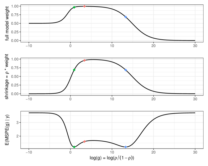
Figure 3: Behavior of $w(g,\bm{Y})$ (top panel), $s(g,\bm{Y})=\rho w(g,\bm{Y})$ (middle panel) and $E(MSPE(g)\mid\bm{Y})$ (bottom panel) as a function of $\log g$. The red diamonds correspond to the local empirical Bayes estimate of $g$; the green and blue diamonds correspond to the values of $g$ that minimize expected mean squared prediction error.

We gain insight into these findings by analyzing, in Figure 4, the behavior of the training data residuals, $\hat{Y}_{i}-Y_{i}$, corresponding to the various values of $\rho$ under consideration. The left panel corresponds to the residuals for the local empirical Bayes value. Aside from the residual for the influential observation, they exhibit a pattern which (while attenuated) mirrors that of the residuals for the constant prediction at the observed mean value plotted in the right panel. Although biased, the residuals corresponding to the optimal $\rho=0.711$, displayed in the middle panel, do not show any pattern. This is in agreement with the previous finding that the expected MSPE is minimized when the prediction line is parallel to the true regression line and supports the intuition that good predictive performance and well behaved residuals go hand in hand.

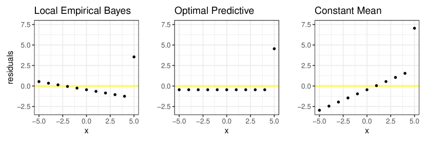
Figure 4: Residuals under three choices of $g$: $g=e^{3.378}$ (left panel), $g=e^{0.901}$ (center panel) and $g=0(\infty)$ (right panel).

3.3 General Mean-shift Contamination

Section 3.2 demonstrated, in a stylized, one-dimensional example, how $g$ could be chosen to minimize prediction error when the training data had been contaminated by a single, influential mean-shift outlier. This section generalizes the result to the setting where multiple candidate predictors exist, the data are contaminated according to the mean-shift contamination described by Abraham and Box (1978), and the response variable is assumed to be observed with error. Suppose the data are generated from the model

$$Y_{i}=\begin{cases}\alpha+\bm{x}_{i}^{T}\bm{\beta}_{True}+\epsilon_{i}+K,&\text{w.p. $\pi$},\\ \alpha+\bm{x}_{i}^{T}\bm{\beta}_{True}+\epsilon_{i},&\text{w.p. $1-\pi$},\end{cases}$$ (7)

where $\epsilon_{i}\stackrel{{\scriptstyle iid}}{{\sim}}N(0,\sigma^{2})$ and $\bm{\beta}_{True}$ is a $p$-dimensional vector which may contain zeros. Let $\bm{X}$ be the $n\times p$ matrix with rows $\bm{x}_{i}^{T}$ and column means zero, and let $\bm{Y}$ be the response vector. Under this model, each case is contaminated independently of the others with probability $\pi$. For simplicity, in this section we assume $\alpha=0$; this assumption does not affect the conclusions we draw.

Assume that for each model $\mathcal{M}_{\gamma}$ we assign Zellner’s $g$ prior to the regression coefficients, $\bm{\beta}_{\gamma}$, and that we allow the scale parameter, $g_{\gamma}$, to differ across models. Denote the collection of scale parameters as $\bm{g}$. For a given prior over the model space, denote the model-averaged estimate of the vector of regression coefficients by $\hat{\bm{\beta}}_{BMA}(\bm{g},\bm{X},\bm{Y})$. With the understanding that this estimate depends on $\bm{g}$, we will refer to this estimate as $\hat{\bm{\beta}}_{BMA}$ for short. Under this model, the vector of model-averaged fitted values is $\hat{\bm{Y}}=\bar{\bm{Y}}+\bm{X}\hat{\bm{\beta}}_{BMA}$.

Suppose future observations $\tilde{\bm{Y}}$ are generated from model (7) using the same design matrix $\bm{X}$ and a possibly different contamination proportion $\tilde{\pi}$. We can examine how the choice of the $g_{\gamma}$ is connected to predictive accuracy by examining the expected sum of squared prediction errors:

$$E(SSPE(\bm{g})\mid\bm{Y},\bm{X}) = E((\tilde{\bm{Y}}-\hat{\bm{Y}})^{T}(\tilde{\bm{Y}}-\hat{\bm{Y}})\mid\bm{X},\bm{Y},\bm{g})$$ (8)

$$= (\hat{\bm{Y}}-E(\tilde{\bm{Y}}))^{T}(\hat{\bm{Y}}-E(\tilde{\bm{Y}}))+$$

$$\hskip 36.135ptE((\tilde{\bm{Y}}-E(\tilde{\bm{Y}}))^{T}(\tilde{\bm{Y}}-E(\tilde{\bm{Y}}))\mid\bm{X},\bm{Y},\bm{g}).$$

The first term in the final expression for the LHS of (8) can be viewed as a squared bias term, while the second term can be viewed as a variance term. The variance term can be shown to be $n\sigma^{2}$, which does not depend on the $g_{\gamma}$, while the squared bias term is

$$(\hat{\bm{Y}}-E(\tilde{\bm{Y}}))^{T}(\hat{\bm{Y}}-E(\tilde{\bm{Y}}))=(\bm{X}\hat{\bm{\beta}}_{BMA}-\bm{X}\bm{\beta}_{True})^{T}(\bm{X}\hat{\bm{\beta}}_{BMA}-\bm{X}\bm{\beta}_{True})+n(\bar{Y}-K\tilde{\pi})^{2}.$$

The term $n(\bar{Y}-K\tilde{\pi})^{2}$ doesn’t depend on the values in $\bm{g}$. If values of $\bm{g}$ exist such that $\hat{\bm{\beta}}_{BMA}=\bm{\beta}_{True}$, those values of $\bm{g}$ would minimize the prediction error. As in the simple case in Section 3.2, a model-averaged regression plane that is parallel to the true mean function will result in optimal predictions as measured by expected $SSPE(\bm{g}\mid\bm{Y},\bm{X})$.

3.4 Variance-inflation Contamination

Suppose the data are generated from the variance-inflation contamination model of Box and Tiao (1968),

$$Y_{i}=\begin{cases}\alpha+\bm{x}_{i}^{T}\bm{\beta}_{True}+\sqrt{K}\epsilon_{i},&\text{w.p. $\pi$},\\ \alpha+\bm{x}_{i}^{T}\bm{\beta}_{True}+\epsilon_{i},&\text{w.p. $1-\pi$},\end{cases}$$ (9)

where $\epsilon_{i}\stackrel{{\scriptstyle iid}}{{\sim}}N(0,\sigma^{2})$. Again, $\bm{\beta}_{True}$ is the $p$-dimensional true regression parameter, which can contain zeros, and we assume $\alpha=0$ to simplify the exposition.

As in Section 3.3, denoting by $\tilde{\pi}$ the contamination proportion in the testing data, $E(SSPE(\bm{g})\mid\bm{X},\bm{Y})$ can be decomposed into a squared bias term and a variance term. The variance term, $n\sigma^{2}(K\tilde{\pi}+1-\tilde{\pi})$, does not depend on $\bm{g}$, while the squared bias term is

$$(\bm{X}\hat{\bm{\beta}}_{BMA}-\bm{X}\bm{\beta}_{True})^{T}(\bm{X}\hat{\bm{\beta}}_{BMA}-\bm{X}\bm{\beta}_{True})+n\bar{Y}^{2}.$$

The conclusion is the same: the BMA regression plane that is parallel to the true regression plane will minimize the expected sum of squared prediction errors, if such a plane exists as a function of $\bm{g}$.

4 Proposed Methods

BMA predictions in regression depend on the posterior distribution over models and on the intra-model estimates of the regression coefficients, all of which depend on the values of $g_{\gamma}$ in Zellner’s $g$ prior. These quantities are sensitive to influential outliers, as demonstrated in the example in Section 3.1. Section 3.2 established, in a simple example, that in the presence of influential outliers prediction error can be minimized if $g$ can be chosen to make the model-averaged regression plane parallel to the true regression plane. Choosing $g$ in this way has the effect of producing well-behaved residuals, which we know from classical regression analysis is desirable. Sections 3.3 and Section 3.4 showed that this intuition holds for more complex model settings.

The intuition developed in Section 3 provides motivation for how one might think about prior specification when there is concern that outliers might impact several (or many) of the models in the ensemble: choose values for the $g_{\gamma}$ to make the model-averaged regression plane parallel to the true regression plane, $\hat{\bm{\beta}}_{BMA}=\bm{\beta}_{True}$. We refer to this as the “parallel condition.” There are two obvious practical limitations to this approach. The first is, of course, that the orientation of the true regression plane is defined by $\bm{\beta}_{True}$, the unknown parameters of the model. The second is that, even if the true $\bm{\beta}_{True}$ were known, there is no guarantee that values $g_{\gamma}$ exist that produce model-averaged coefficients satisfying the parallel condition. This can be illustrated simply in the context of the example in Section 3.2 by taking $K=5$ instead of $K=-5$. When $K=5$, the least squares estimate of the slope is $\hat{\beta}_{LS}=0.2727$. As a function of $g$, the shrinkage coefficient $s(g,\bm{Y})=(g/(1+g))w(g,\bm{Y})$ ranges between zero and one, and so there is no value of $g$ that produces $\hat{\beta}_{BMA}=s(g,\bm{Y})\hat{\beta}_{LS}$ equal to $\beta=0.5$. This extends to the general setting where $p>1$. In this case the model-averaged estimate of the coefficient corresponding to regressor $X_{j}$ is

$$\hat{\beta}_{BMA,j}=\sum_{\gamma\in\Gamma\;:\;X_{j}\in\mathcal{M}_{\gamma}}\left(\frac{g_{\gamma}}{1+g_{\gamma}}\right)\hat{\beta}_{LS,\gamma,j}\pi(\mathcal{M}_{\gamma}\mid\bm{Y}),$$

where $\hat{\beta}_{LS,\gamma,j}$ is the least squares estimate of $\beta_{j}$ in a model $\mathcal{M}_{\gamma}$ that contains $X_{j}$ as a regressor. The terms $\hat{\beta}_{LS,\gamma,j}$ do not depend on the $g_{\gamma}$ and can be bounded above and below by their largest and smallest values across the model space. The terms $(g_{\gamma}/(1+g_{\gamma}))\pi(\mathcal{M}_{\gamma}\mid\bm{Y})$ depend on the $g_{\gamma}$ but are bounded below and above by zero and one, hence there is no guarantee that there exist values of $g_{\gamma}$ that will produce a regression plane that is parallel to the true regression plane with $\hat{\beta}_{BMA,j}=\hat{\beta}_{True,j}$, for $j=1,\ldots,p$.

In this section we address these practical limitations in several ways. First, in Section 4.1, we expand the space of prior distributions so that the parallel condition is achievable for a larger space of observed data sets than is possible under Zellner’s $g$ prior that shrinks toward zero. Second, in Section 4.2 we relax the strict parallel condition by attempting to find values of the model’s hyperparameters that make the model-averaged regression plane as close to parallel to the true regression plane as possible in $L_{2}$ distance. Finally, in Section 4.3 we synthesize these ideas and propose an approach for choosing empirically the values of the model’s hyperparameters with the goal of yielding small prediction error in the presence of influential outliers. As the orientation of the true regression plane is unknown, we propose using robust estimates that are insensitive to influential outliers as part of the procedure for choosing the hyperparameters.

4.1 Expanding the Prior Model

For particular data and true model settings there may not exist values $g_{\gamma}$ under Zellner’s $g$ prior (1) which shrinks all coefficients toward zero that satisfy $\hat{\bm{\beta}}_{BMA}=\bm{\beta}_{True}$. When this is the case, we might instead chose values $g_{\gamma}$ that make the model-averaged regression plane as close to parallel as possible to the true regression plane. To improve the quality of this approximation, we expand the prior model to allow for shrinkage toward a potentially non-zero target, $\bm{\theta}_{\gamma}$. Under this prior, described in (3), the model-averaged estimate of the coefficient corresponding to regressor $X_{j}$ is

$$\hat{\beta}_{BMA,j}=\sum_{\gamma\in\Gamma\;:\;X_{j}\in\mathcal{M}_{\gamma}}\left(\frac{1}{1+g_{\gamma}}\theta_{\gamma,j}+\frac{g_{\gamma}}{1+g_{\gamma}}\hat{\beta}_{LS,\gamma,j}\right)\pi(\mathcal{M}_{\gamma}\mid\bm{Y}).$$

The hyperparameters $\bm{\theta}_{\gamma}$ provide extra flexibility that allows for shrinkage toward targets other than zero. To set notation, let $\{\bm{\theta}_{\gamma},g_{\gamma}\}$ denote the hyperparameters for model $\mathcal{M}_{\gamma}$ and let $\{\bm{\Theta},\bm{g}\}$ denote the collection of hyperparameters $\bm{\theta}_{\gamma}$ and $g_{\gamma}$ across all models indexed by $\gamma\in\Gamma$. By enlarging the collection of hyperparameters from $\bm{g}$ to $\{\bm{\Theta},\bm{g}\}$, we are able to achieve the parallel condition, $\hat{\bm{\beta}}_{BMA}=\bm{\beta}_{True}$, for a wider range of data and true model settings.

This can be seen clearly in a modified version of the example in Section 3.2 where $K=5$ and the true regression coefficient is $\beta=2$. When shrinking toward a prior mean of zero, no value of $g$ is able to produce $\hat{\beta}_{BMA}=\beta$ because $\hat{\beta}_{LS}=1.7727$ and $\beta=2>\hat{\beta}_{LS}$. However, when shrinking toward a potentially non-zero prior mean $\theta$, there are many such $\{\theta,g\}$ pairs that produce $\hat{\beta}_{BMA}=2$, and we can chose a pair according to some rule (e.g., favoring small values of $\theta$ to encourage shrinkage toward zero, or discouraging small values of $g$ to avoid overconfidence in the prior). The added flexibility of shrinking toward a non-zero mean $\theta$ does not guarantee we can achieve the parallel condition, e.g., when $\beta=0.5$ and $K=5$ in the example in Section 3.2, there are no $\{\theta,g\}$ pairs that produce $\hat{\beta}_{BMA}=0.5$. The added flexibility, though, means we can do no worse than shrinking toward zero if our goal is to bring the model-averaged prediction plane as close to parallel to the true regression plane as possible, and so we work with prior (3) from now on.

4.2 Relaxing the Parallel Condition: The Overall-Mixture Prior Specification

Even after expanding the space of priors to include non-zero prior means $\bm{\theta}_{\gamma}$, the parallel condition is not guaranteed to be achievable for all data sets. To address this issue, we might relax the parallel condition and choose hyperparameter values $\{\bm{\Theta},\bm{g}\}$ so that the model-averaged regression plane is as close in $L_{2}$ distance as possible to the true regression plane:

$$\{\hat{\bm{\Theta}},\hat{\bm{g}}\}=\underset{\bm{\Theta},\bm{g}}{\arg\min}\,|\!|\hat{\bm{\beta}}_{BMA}-\bm{\beta}_{True}|\!|^{2}.$$ (10)

This defines an empirical Bayes approach for selecting hyperparameter values that could be implemented if $\bm{\beta}_{True}$ were known or replaced with a suitable estimate. We call this approach the overall-mixture prior specification. The main difficulty in implementing (10) in practice is computational: with $p$ predictors, there are $(2^{p}-1)+(p2^{p-1})$ total hyperparameters: $2^{p}-1$ scale parameters $g_{\gamma}$ and $\sum_{k=0}^{p}k{p\choose k}=p2^{p-1}$ individual location parameters $\theta_{\gamma,k}$, where $\theta_{\gamma,k}$ is the $k$th elements of the prior mean vector for model $\mathcal{M}_{\gamma}$. Not only does this represent a high-dimensional optimization problem, but for any given collection of values $\{\bm{\Theta},\bm{g}\}$ calculating $\hat{\bm{\beta}}_{BMA}$ requires summing over $2^{p}$ models, where each term in the sum contains non-linear functions of elements of $\{\bm{\theta}_{\gamma},g_{\gamma}\}$. Brute-force, numerical optimization approaches might be feasible in very small problems, but will be challenging in general. If interest is limited to point prediction under posterior predictive $L_{2}$ loss and the the parallel condition can be achieved, predictions based on the resulting $\hat{\bm{\beta}}_{BMA}$ would coincide with predictions based directly on ${\bm{\beta}}_{True}$.

4.3 Local Null-Mixture Prior Specification

To ease the computational burdens discussed in Section 4.2 while still using the parallel condition to our advantage, we propose a new local empirical Bayes approach for hyperparameter specification. The approach is “local” in that each model receives its own, unique hyperparameter values $\{\bm{\theta}_{\gamma},g_{\gamma}\}$ and also in that the selection of values for the hyperparameters requires calculations that are dependent only on that model. In principle, this is similar to the local empirical Bayes approach, though our criterion for specifying the hyperparameter values is motivated by the parallel condition (rather than by maximization of the marginal likelihood).

Rather than focusing on the full model-averaged regression plane defined by $\hat{\bm{\beta}}_{BMA}$ in (10), which requires knowledge about all $2^{p}$ models in $\Gamma$, for any given model $\mathcal{M}_{\gamma}$ we focus solely on the relationship between the model $\mathcal{M}_{\gamma}$ and the null model with no predictors, $\mathcal{M}_{N}$. If the only two models under consideration were $\mathcal{M}_{\gamma}$ and $\mathcal{M}_{N}$, the posterior probability of model $\mathcal{M}_{\gamma}$ would be

$$\pi^{*}(\mathcal{M}_{\gamma}\mid\bm{Y})=\left(1+\frac{m(\bm{Y}\mid\mathcal{M}_{N})}{m(\bm{Y}\mid\mathcal{M}_{\gamma})}\frac{\pi^{*}(\mathcal{M}_{N})}{\pi^{*}(\mathcal{M}_{\gamma})}\right)^{-1}=\left(1+\frac{1}{BF(\mathcal{M}_{\gamma}:\mathcal{M}_{N})}\frac{\pi^{*}(\mathcal{M}_{N})}{\pi^{*}(\mathcal{M}_{\gamma})}\right)^{-1},$$

where $BF(\mathcal{M}_{\gamma}:\mathcal{M}_{N})$ is the Bayes factor for comparing model $\mathcal{M}_{\gamma}$ to the null model given in Equation (5). We use $\pi^{*}(\mathcal{M}_{N})$ and $\pi^{*}(\mathcal{M}_{\gamma})$ to denote the assigned prior model probabilities when the model space contains only the two models $\mathcal{M}_{N}$ and $\mathcal{M}_{\gamma}$. As a default, we use $\pi^{*}(\mathcal{M}_{N})=\pi^{*}(\mathcal{M}_{\gamma})=0.5$, which is also what would result from using the uniform prior or the Beta-Binomial$(1,1)$ prior over a model space that contains only these two models. The model-averaged estimate of $\bm{\beta}_{\gamma}$ when the only two models in the model space are $\mathcal{M}_{N}$ and $\mathcal{M}_{\gamma}$ is

$$\hat{\bm{\beta}}_{BMA,\gamma}=\pi^{*}(\mathcal{M}_{\gamma}\mid\bm{Y})\left(\frac{1}{1+g_{\gamma}}\bm{\theta}_{\gamma}+\frac{g_{\gamma}}{1+g_{\gamma}}\hat{\bm{\beta}}_{LS,\gamma}\right),$$

where $\hat{\bm{\beta}}_{LS,\gamma}$ is the least squares estimate of $\bm{\beta}_{\gamma}$. The relaxed parallel condition in (10) then tells us to choose hyperparameter values that satisfy

$$\{\hat{\bm{\theta}}_{\gamma},\hat{g}_{\gamma}\}=\underset{\{\bm{\theta}_{\gamma},g_{\gamma}\}}{\arg\min}\,|\!|\hat{\bm{\beta}}_{BMA,\gamma}-\bm{\beta}_{True,\gamma}|\!|^{2},$$ (11)

where $\bm{\beta}_{True,\gamma}$ is interpreted here as the true regression coefficients for model $\mathcal{M}_{\gamma}$. Once hyperparameters for each of the $2^{p}-1$ models have been found via (11), model-averaged prediction proceeds as usual using the posterior model probabilities $\pi(\mathcal{M}_{\gamma}\mid\bm{Y})$ computed under the original prior $\pi(\mathcal{M}_{\gamma})$ over the entire, unrestricted model space, $\Gamma$.

The local null-mixture approach for selecting hyperparameter values defined in (11) attempts to make the locally-model-averaged regression plane parallel to an unknown regression plane oriented according to $\bm{\beta}_{True,\gamma}$. In practice, we require estimates of these unknown parameters. We opt to use an estimate of $\bm{\beta}_{True,\gamma}$ that is robust in the sense that is relatively insensitive to influential outliers (see Rousseeuw and Leroy, 2005, for a general treatment of robust regression). For a given model $\mathcal{M}_{\gamma}$, we rank each observation according to its Cook’s distance, $D_{i,\gamma}$ (Cook, 1977). We then remove 10% of the cases corresponding to the largest values of Cook’s distance, and compute the ordinary least squares estimate of the regression coefficients using the remaining 90% of the cases. With this robust estimate, $\hat{\bm{\beta}}_{Robust,\gamma}$, in hand, we choose hyperparameters for model $\mathcal{M}_{\gamma}$ that satisfy the criterion

$$\{\hat{\bm{\theta}}_{\gamma},\hat{g}_{\gamma}\}=\underset{\{\bm{\theta}_{\gamma},g_{\gamma}\}}{\arg\min}\,|\!|\hat{\bm{\beta}}_{BMA,\gamma}-\hat{\bm{\beta}}_{Robust,\gamma}|\!|^{2}_{2}.$$

We use the optim function in R (R Core Team, 2021) to implement this approach in the examples in Section 5.

The local null-mixture approach is attractive due to the fact that it reduces the computational burden associated with criterion (10). However, because the hyperparameters are chosen locally—by mixing models $\mathcal{M}_{\gamma}$ and $\mathcal{M}_{N}$—rather than globally—by averaging over all models in (10)—the predictive optimally associated with the parallel condition is not guaranteed. However, based on the intuition developed in Section 3.2, choosing hyperparameters locally will still result in well-behaved residuals that are local to the mixture of the models $\mathcal{M}_{\gamma}$ and $\mathcal{M}_{N}$. As good prediction and well-behaved residuals tend to go hand-in-hand, we expect the local null-mix method to perform well in practice. In addition, as the simulations in Section 5 will demonstrate, this local approach can outperform the global approach when some of the true regression parameters $\beta_{j}$ are equal to zero.

5 Simulations

In this section we present simulation studies comparing the predictive performance of our proposed method to that of the related methods mentioned in Section 2: local empirical Bayes (EB-Local), global empirical Bayes (EB-Global), and the hyper-$g/n$ methods. The computations for the related methods were performed using the BAS package in R (Clyde, 2020). The $\mbox{Beta-Binomial}(1,1)$ prior over the model space with $\pi(\mathcal{M}_{\gamma})=(p+1)^{-1}{p\choose|\mathcal{M}_{\gamma}|}^{-1}$ was used for each of the BMA methods. We also compare the performance of the BMA predictions to the performance of predictions based on the robust estimate $\hat{\bm{\beta}}_{Robust,\gamma}$ described in Section 4.3 under the full model with $\gamma=(1,\ldots,1)^{T}$ (i.e., no model averaging).

In real-world settings, data contamination may constitute a one-off occurrence or it may represent a structural component of the underlying stochastic mechanism (a fraction of the observations may follow a different distribution than the bulk of the observations). In the first case we might expect only the training (or only the testing) data to be contaminated. In the second case we would expect both the training and the testing data to be contaminated. Our simulations evaluate the performance of the different methods in both of these cases, as well as in the case when neither the training nor the testing data are contaminated. We consider contaminations arising from a mean-shift and from a variance-inflation scheme. The data contamination patterns for the five simulations we conducted are summarized in Table 1.

	contamination pattern
	M-S/no	M-S/M-S	V-I/no	V-I/V-I	no/no
training data	M-S	M-S	V-I	V-I	no
testing data	no	M-S	no	V-I	no

Table 1: Data contamination patterns for the training and testing data used in the simulations: mean-shift (M-S), variance-inflation (V-I), and no contamination (no).

	$p=5$						$p=10$
	complexity level						complexity level
	1	2	3	4	5		1	5	10
$\beta_{1}=$	1	1	1	1	1		0.5	0.5	0.5
$\beta_{2}=$	0	2	2	2	2		0.0	1.0	1.0
$\beta_{3}=$	0	0	3	3	3		0.0	1.5	1.5
$\beta_{4}=$	0	0	0	4	4		0.0	2.0	2.0
$\beta_{5}=$	0	0	0	0	5		0.0	2.5	2.5
$\beta_{6}=$							0.0	0.0	3.0
$\beta_{7}=$							0.0	0.0	3.5
$\beta_{8}=$							0.0	0.0	4.0
$\beta_{9}=$							0.0	0.0	4.5
$\beta_{10}=$							0.0	0.0	5.0

Table 2: The columns in the left-hand side of the table display the values of $\bm{\beta}=(\beta_{1},\beta_{2},\beta_{3},\beta_{4},\beta_{5})^{T}$ for the five models of increasing complexity used in the simulations with $p=5$. The columns in the right-hand side of the table display the values of $\bm{\beta}=(\beta_{1},\ldots,\beta_{10})^{T}$ for the three models of increasing complexity used in the simulations with $p=10$.

Prior to possibly being contaminated, the training and the testing data are both generated from the true model

$$\begin{split}\bm{Y}_{Train}&=\bm{X}_{Train}\bm{\beta}+\alpha\bm{1}+\bm{\epsilon},\\ \bm{Y}_{Test}&=\bm{X}_{Test}\bm{\beta}+\alpha\bm{1}+\bm{\epsilon}.\end{split}$$

For simplicity, in all simulations, we set $\alpha=0$. The design matrices $\bm{X}_{Train}$ and $\bm{X}_{Test}$ have dimension $100\times 5$ and their rows are independently generated from a multivariate normal distribution, MVN$(\bm{0},\bm{\Sigma})$, where the covariance matrix $\bm{\Sigma}$ has diagonal elements equal to $1$ and off-diagonal elements equal to $0.6$. The error vector $\bm{\epsilon}$ has i.i.d. standard normal random elements.

In the mean-shift case, we contaminate the data by randomly selecting 5% of the observations and adding $K=10$ to the dependent variable. In the variance-inflation case, we contaminate the data by randomly selecting 5% of the observations and multiplying their errors, $\epsilon_{i}$, by $\sqrt{10}$ before adding them to the mean function so that the errors for the contaminated cases have variance $K=10$. To assess how model complexity affects performance we consider five models of increasing complexity where the number of active predictors ranges from one to five. The values of the vectors of regression coefficients $\bm{\beta}$ for the five models are summarized in the left-hand side of Table 2.

For settings where the training data are contaminated, we use either the mean-shift scheme or the variance-inflation scheme to contaminate the training data set. For the testing data, we either contaminate it with the same scheme used to contaminate the training data set or we leave it uncontaminated. Therefore, we have multiple settings based on the true coefficients and the contamination scheme of the training and testing data sets. Since we have 5 true $\bm{\beta}$ vectors and 5 different contamination combinations, we have 25 different settings in total.

Our simulations consider all $5\times 5=25$ settings resulting from pairing one of the 5 data contamination patterns with one of the 5 model complexity levels. In each of these settings, we simulate 500 training and testing data sets to evaluate the performance of the different methods mentioned at the start of the section. We apply each method to the training data sets to estimate models and let the models make predictions $\bm{\hat{Y}}$ for the testing data sets. Specifically, the BMA predictions $\bm{\hat{Y}}$ are calculated according to the following steps.

1. Centering the training data: We use $\bm{X}_{Train,c}$ to denote the centered training design matrices, and $\bm{X}_{Train,mean}$ to denote the corresponding column mean vector, i.e.,

   $$\bm{X}_{Train,c}=\bm{X}_{Train}-\bm{1}\,\bm{X}_{Train,mean}^{T},$$

   where $\bm{1}$ is a vector of size $n$ with all the elements equal to 1.

2. Fitting models to the training data sets: By applying each of the BMA methods, indexed by $m$, to the centered training data sets $(\bm{Y}_{Train},\bm{X}_{Train,c})$ we obtain fitted BMA planes:

   $$\bm{\hat{Y}}_{Train,m}=\bm{1}\,\bar{\bm{Y}}_{Train}+\bm{X}_{Train,c}\,\bm{\hat{\beta}}_{BMA,m},$$

   where $\bm{\hat{\beta}}_{BMA,m}$ is the BMA estimate of $\bm{\beta}$ for method $m$, $\bar{\bm{Y}}_{Train}$ is the average of $\bm{Y}_{Train}$ (which is also the estimated intercept), and $\bm{\hat{Y}}_{Train,m}$ are the values predicted by method $m$ for the training data.

3. Making predictions: We employ the estimated parameters from the previous step to construct the following prediction plane:

   $$\hat{\bm{Y}}_{m}=\bm{1}\,\bar{\bm{Y}}_{Train}+\left(\bm{X}_{Test}-\bm{1}\,\bm{X}_{Train,mean}^{T}\right)\bm{\hat{\beta}}_{BMA,m}.$$

   By subtracting the column means of the training design matrix from the testing design matrix we ensure that the estimated model parameters can be meaningfully applied to the testing data.

In each of the 25 simulation settings and for each method $m$, after acquiring the predictions $\bm{\hat{Y}}_{m}^{(i)}$ for replication $i$, $i=1,\ldots,500$, we compute the observed MSPE for that iteration as

$$\text{MSPE}_{m}^{(i)}=\frac{1}{n}\left\|{\bm{\hat{Y}}}_{m}^{(i)}-\bm{Y}_{Test}^{(i)}\right\|^{2},$$

where $n$ is the number of observations in the testing data set (here $n=100$). We are mainly interested in assessing the relative performance of the various methods. To this end, for replication $i$, letting $m^{*}$ denote the hyper-$g/n$ method that we take as a reference, we compute the relative percent reduction in MSPE for the other methods relative to $m^{*}$ as

$$\text{RR}_{m,m^{*}}^{(i)}=100\times\frac{\text{MSPE}_{m^{*}}^{(i)}-\text{MSPE}_{m}^{(i)}}{\text{MSPE}_{m^{*}}^{(i)}},\,\,\,i=1,\ldots,500.$$

The relative percent reduction in MSPE values from 500 replications for each of the 25 simulation settings are summarized graphically in the boxplots of Figure 5. First, we note that the two empirical Bayes BMA methods both perform similarly to the hyper-$g/n$ BMA method. Comparing the local null-mixture method to the other BMA methods, perhaps the most conspicuous finding is that, when the training data are contaminated and the testing data are uncontaminated, the proposed method exhibits the largest relative improvements over the competing BMA methods for both contamination schemes (when making visual comparisons, note that the scale on the vertical axes differ across panels). The relative improvements are smaller in settings when both the training and the testing data are contaminated. The variability of the proposed method appears to increase with model complexity. In particular, when the complexity level equals 5, the relative performance of the proposed method can be significantly worse in a small number of replications. The bottom panel in the figure shows that the proposed methodology suffers a little compared to the other BMA methods when the training data are uncontaminated. This behavior is to be expected and suggests that the methodology is best suited for situation in which the analyst suspects that contamination is present, although the median performance deterioration in the case of no contamination is tolerable.

It follows from the last remark in Section 4.2 that, when the parallel condition can be achieved, predictions based directly on $\hat{\bm{\beta}}_{Robust,\gamma}$, the robust estimate of ${\bm{\beta}}_{True}$ under the full model, coincide with the predictions produced by the overall-mixture method under posterior predictive $L_{2}$ loss. Compared to the local null-mixture method, the performance of the robust (overall-mixture) predictions varies with the complexity of the underlying, true, uncontaminated model.

When the true complexity is less than $p$, the performance of the overall-mixture method suffers from its strong reliance on the robust estimate under an overparameterized model and the attendant loss of accuracy from estimation of the $\beta_{j}$ coefficients equal to zero. By contrast, the local null-mixture model attains higher precision because it builds upon separate robust estimates for all possible models including the model that excludes the $\beta_{j}$ equal to zero. This is evidenced by the reduced variability exhibited by the boxplots (local null-mixture vs. robust) for smaller complexity settings in Figure 5.

While less variable overall, the EB-Global and EB-Local methods tend to underperform relative to the local null-mixture and the robust method whenever any contamination is present. When neither the trainig nor the testing data are contaminated, the EB-Global and EB-Local methods exhibit better predictive performance. In such cases, the local null-mixture method outperforms the robust approach when the complexity is small relative to $p$, and does about as well as the robust approach when the complexity matches $p$.

In summary, these results suggest that, in the realistic situation when there is uncertainty about model composition, the local null-mixture method is preferable to the the robust method from a predictive perspective and has the additional advantage of providing posterior descriptions of uncertainty about variable inclusion and other aspects of the posterior and predictive distributions.

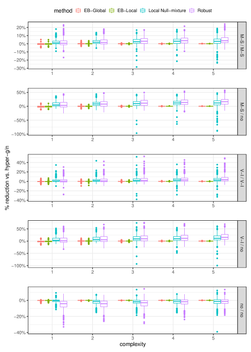
Figure 5: Percent reduction in MSPE relative to the model-averaged hyper-$g/n$ method for the simulation study with $p=5$ predictors under complexity settings (the number of non-zero coefficients) ranging from 1 to 5. Each row corresponds to a contamination scheme, labeled “X / Y”, where X (Y) denotes the contamination scheme for the training (test) data. “M-S” denotes mean-shift contamination, “V-I” denotes variance-inflation contamination, and “no” denotes no contamination.

We performed a second simulation study to demonstrate how the predictive performance of the local null-mixture method scales in comparison to the other methods as $p$ increases. The setup is the same as above but now with double the number of predictors ($p=10$) and three complexity settings (1, 5 and 10). The values of the true coefficients $\bm{\beta}=(\beta_{1},\ldots,\beta_{10})^{T}$ under each of the three complexity settings are given in the right-hand side of Table 2. The results, summarized graphically in Figure 6, confirm the overall features and patterns uncovered by the first simulation study.

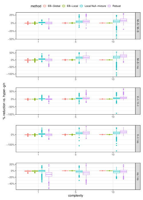
Figure 6: Percent reduction in MSPE relative to the model-averaged hyper-$g/n$ method for the simulation study with $p=10$ predictors under complexity settings (the number of non-zero coefficients) 1, 5 and 10. Each row corresponds to a contamination scheme, labeled “X / Y”, where X (Y) denotes the contamination scheme for the training (test) data. “M-S” denotes mean-shift contamination, “V-I” denotes variance-inflation contamination, and “no” denotes no contamination.

6 Crime Data

To evaluate the out-of-sample predictive performances of several of the methods discussed in this article in a real data analysis setting, we consider the crime data reported in Agresti and Agresti (1970). The methods we evaluate are a subset of those considered in the simulation study (Hyper-$g/n$, EB-Local, EB-Global, and Local Null-mixture), and we again use the Beta-Binomial$(1,1)$ prior over the model space.

For each US state and the District of Columbia, the data comprise a dependent variable, “violent crimes per 100,000 people,” to be modeled in terms of eight socio-economic regressors. Following a preliminary exploratory analysis we took a logarithmic transformation of the dependent variable to remedy the skewness of the observed counts. In addition, the exploratory analysis uncovered positive correlations between the transformed dependent variable and some of the regressors as well as between some of the regressors themselves. Diagnostics for the full linear regression model revealed that the observations for Hawaii (HI) and the District of Columbia (DC) are the most highly influential and that a normality assumption for the errors in the full model might not hold. We also examined residual plots produced by applying various BMA procedures to the data and found that the residuals for the three traditional methods EB-Local, EB-Global, and Hyper-$g/n$, are very similar but differ in several aspects from those of the local null-mixture method (e.g., the local null-mixture method produces a larger residual for Alaska (AK) and a smaller one for DC).

We used $K$-fold cross-validation (Friedman et al., 2001) to evaluate the out-of-sample predictive performance of the various methods, executing the following steps: (a) partition the observations at random into $K$ subsets having approximately equal size; (b) conditional on the selected partition, leave out in turn one of the $K$ subsets as the testing data, and use the remaining $K-1$ subsets as the training data; (c) apply the various BMA methods to the training data to make predictions on the testing data.

Using the cross-validated predictions, the cross-validation error (CVE) of each method, is calculated as

$$CV\!E(\hat{f},\text{method},K,\mathcal{P})=\frac{1}{n}\sum_{i=1}^{n}\left(Y_{i}-\hat{f}^{\setminus\kappa(i)}(\bm{X_{i}},\text{method})\right)^{2},$$ (12)

where $n$ is the number of observations in the data set, $K$ is the number of sets in the selected partition $\mathcal{P}$, $\kappa(i)$ denotes the held-out element of the partition $\mathcal{P}$ to which observation $i$ belongs, and $\hat{f}^{\setminus\kappa(i)}(\bm{X_{i}},\text{method})$ denotes the fitted value at $\bm{X_{i}}$ produced by a given method when the $\kappa(i)$-th element of the partition is removed.

For given $K$, the CVE value varies from partition to partition and, assuming a uniform distribution over partitions, we can define an expected cross-validation error (ECVE). When $K=51$, there is only one partition and the ECVE can be computed exactly using Equation (12). For smaller values of $K$, when there are too many partitions to compute the exact expectation, we repeat the $K$-fold cross-validation procedure $T$ times and approximate the ECVE by

$$\widehat{ECV\!E}(\hat{f},\text{method},K)=\frac{1}{T}\sum_{t=1}^{T}\left(CV\!E(\hat{f},\text{method},K,\mathcal{P}^{(t)})\right),$$ (13)

where $\mathcal{P}^{(t)}$ represents a partition selected at random in repetition $(t)$.

The cross-validation results for values of $K$ equal to 51, 25, and 10 are summarized in Table 3. The EB-Local and EB-Global methods always perform comparably to one another and slightly better than the Hyper-$g/n$ method. The Local Null-mixture method clearly outperforms all other methods for $K$ equal to 51, is noticeably better for $K$ equal to 25, and is only slightly worse for $K$ equal to 10.

	$K=51$		$K=25$		$K=10$
Method	$ECV\!E$	% Red.	$\widehat{ECV\!E}$	% Red.	$\widehat{ECV\!E}$	% Red.
Hyper-$g/n$	0.204	$\cdot$	0.204	$\cdot$	0.209	$\cdot$
EB-Local	0.202	0.94	0.203	0.93	0.207	0.91
EB-Global	0.202	1.17	0.202	1.16	0.207	1.11
Local Null-mixture	0.174	14.73	0.197	3.87	0.218	-4.40

Table 3: For the crime data, $ECV\!E$ and $\widehat{ECV\!E}$ for various BMA methods and the realized percent reduction in their values compared to those obtained using the Hyper-$g/n$ method. The largest realized percent reduction for each cross-validation setting $K$ appears in boldface.

The two most influential cases (DC and HI) have a similar impact on the full model. Apparently, the Local Null-mixture method benefits from the inclusion of one of these two cases in the training set and of the other in the testing set. This happens with probability one when $K$ equals 51 and with decreasing probability as $K$ becomes larger.

7 Discussion

We developed BMA model prediction methodology for common types of regression model misfit, in particular the presence of influential observations and non-constant residual variance. The methodology is motivated by the view that, typically, good predictive performance cannot be attained unless the model residuals are well behaved. The regression models under consideration make use of variants on Zellner’s $g$ prior. By studying the impact of various forms of model misfit on BMA predictions in simple situations we were able to identify prescriptive guidelines for “tuning” Zellner’s $g$ prior to obtain optimal predictions. The methodology can be thought of as an “empirical Bayes” approach to modeling, as the data help to inform the specification of the prior in an attempt to attenuate the negative impact of model misfit. The methods described in the paper can be extended to other types of model misfit, such as non-linearity of the mean function (or model under-fit), and can be implemented with different adaptations of robust $g$-prior specification, as illustrated in Wang (2016).

In modern applications, especially when there are many potential predictor variables, analysts do not have the time (or, due to the size of the problem, are not able) to interactively investigate the quality of fitted models, hampering one’s ability to manually attenuate the impact of model misfit through either model revision or prior tuning. In such complex situations, the guidelines developed in the simple examples considered in this paper can motivate automatic or semi-automatic procedures that provide some insurance against Bayesian predictions that are unduly impacted by gross model specification.

Standard implementations of BMA analyses based on Zellner’s $g$ prior typically make the simplifying assumption that the prior mean of the regression coefficients is zero, leading to shrinkage of the least squares estimate toward the origin, which may be sub-optimal in the presence of model misfit. By developing BMA strategies that take advantage of the full generality of the prior as proposed by Zellner, in particular by allowing for a non-zero prior mean, we are able to achieve shrinkage toward points other than the origin, which can have the effect of attenuating the impact of model misfit on prediction. There is little doubt that our proposed methodology may not be as good as the best possible human analysis (with the understanding, of course, that the quality of such an analysis depends on the skills of the individual analyst), but we have demonstrated through theoretical arguments and empirical investigations that our methodology performs better than routine implementations of BMA that do not account for model misfit.

In our methodology, the tuning of the prior distribution is obtained by considering theoretical properties that should be enjoyed by the optimal fit (mainly, the parallel condition) of the various models in the BMA ensemble. This approach should lead to well-behaved residuals for each of the individual models. An alternative approach to fine-tuning the prior distributions could focus on the realized residuals of the model-averaged fit. This would be a more empirical approach requiring an objective function that assesses quantitatively the quality of the realized residuals coupled with a feasible computational approach for sequentially updating the prior parameters to improve such an objective function. An appeal of such an approach is the potential for the development of dynamic, graphical diagnostics that are closely related to the traditional diagnostics for linear regression that are familiar to most users.

Finally, extension of our methods to situations involving very large data sets may require the development of algorithms that implement computational shortcuts for the determination of the prior tuning parameters. A guiding direction for such work would be to develop shortcuts that, while speeding up computation, do not unduly compromise the Bayesian optimality guarantees implicit in our framework.

Acknowledgments.

This work was supported by the National Science Foundation under awards No. DMS-1310294, No. SES-1424481, and No. SES-1921523. The manuscript is based on the third author’s Ph.D. dissertation completed at The Ohio State University.

References

- Abraham and Box (1978) Abraham, B. and Box, G. E. (1978). Linear Models and Spurious Observations. Applied Statistics, pages 131–138.
- Agresti and Agresti (1970) Agresti, A. and Agresti, B. F. (1970). Statistical Methods for the Social Sciences. CA: Dellen Publishers.
- Barbieri and Berger (2004) Barbieri, M. and Berger, J. O. (2004). Optimal predictive model selection. The Annals of Statistics, 32, 870–897.
- Bayarri et al. (2012) Bayarri, M. J., Berger, J. O., Forte, A., and García-Donato, G. (2012). Criteria for Bayesian model choice with application to variable selection. The Annals of Statistics, 40, 1550–1577.
- Berger et al. (1998) Berger, J. O., Pericchi, L. R., and Varshavsky, J. A. (1998). Bayes factors and marginal distributions in invariant situations. Sankhyā, Ser. A, 60, 307–321.
- Bernardo and Smith (1994) Bernardo, J. M. and Smith, A. F. M. (1994). Bayesian Theory. John Wiley & Sons, New York; Chichester.
- Box and Tiao (1968) Box, G. E. and Tiao, G. C. (1968). A Bayesian approach to some outlier problems. Biometrika, 55(1), 119–129.
- Carvalho and Lawrence (2008) Carvalho, L. E. and Lawrence, C. E. (2008). Centroid estimation in discrete high-dimensional spaces with applications in biology. Proceedings of the National Academy of Sciences, 105, 3209–3214.
- Chaloner and Brant (1988) Chaloner, K. and Brant, R. (1988). A Bayesian approach to outlier detection and residual analysis. Biometrika, 75(4), 651–659.
- Chipman et al. (2001) Chipman, H. A., George, E. I., and McCulloch, R. E. (2001). The practical implementation of Bayesian model selection (with discussion). In P. Lahiri, editor, Model Selection, pages 65–134. IMS, Beachwood, OH.
- Clyde (2020) Clyde, M. (2020). BAS: Bayesian Variable Selection and Model Averaging using Bayesian Adaptive Sampling. R package version 1.5.5.
- Clyde and George (2004) Clyde, M. and George, E. I. (2004). Model uncertainty. Statistical Science, 19, 81–94.
- Clyde et al. (2011) Clyde, M., Ghosh, J., and Littman, M. (2011). Bayesian adaptive sampling for variable selection. Journal of Computational and Graphical Statistics, 20, 80–101.
- Clyde (2001) Clyde, M. A. (2001). Discussion of “The practical implementation of Bayesian model selection” by H. A. Chipman, E. I. Geroge and R. E. McCulloch. In P. Lahiri, editor, Model Selection, pages 117–124. IMS, Beachwood, OH.
- Clyde and George (2000) Clyde, M. A. and George, E. I. (2000). Flexible empirical Bayes estimation for wavelets. Journal of the Royal Statistical Society, Ser. B, 62, 681–698.
- Cook (1977) Cook, R. D. (1977). Detection of influential observation in linear regression. Technometrics, 19, 15–18.
- Cook and Weisberg (1982) Cook, R. D. and Weisberg, S. (1982). Residuals and influence in regression. New York: Chapman and Hall.
- Cui and George (2008) Cui, W. and George, E. I. (2008). Empirical Bayes vs. fully Bayes variable selection. Journal of Statistical Planning and Inference, 138, 888–900.
- Fernández et al. (2001) Fernández, C., Ley, E., and Steel, M. (2001). Benchmark priors for Bayesian model averaging. Journal of Econometrics, 100, 381–427.
- Foster and George (1994) Foster, D. P. and George, E. I. (1994). The risk inflation criterion for multiple regression. Annals of Statistics, 22, 1947–1975.
- Friedman et al. (2001) Friedman, J., Hastie, T., Tibshirani, R., et al. (2001). The Elements of Statistical Learning, volume 1. New York: Springer.
- George and Foster (2000) George, E. and Foster, D. (2000). Calibration and empirical Bayes variable selection. Biometrika, 87(4), 731–747.
- George and McCulloch (1993) George, E. I. and McCulloch, R. E. (1993). Variable selection via Gibbs sampling. Journal of the American Statistical Association, 88, 881–889.
- George and McCulloch (1997) George, E. I. and McCulloch, R. E. (1997). Approaches for Bayesian variable selection. Statistica Sinica, 7, 339–373.
- Hans et al. (2007) Hans, C., Dobra, A., and West, M. (2007). Shotgun stochastic search for “large ” regression. Journal of the American Statistical Association, 102, 507–516.
- Hansen and Yu (2001) Hansen, M. H. and Yu, B. (2001). Model selection and the principle of minimum description length. Journal of the American Statistical Association, 96, 746–774.
- Hoeting et al. (1996) Hoeting, J., Raftery, A. E., and Madigan, D. (1996). A method for simultaneous variable selection and outlier identification in linear regression. Computational Statistics & Data Analysis, 22(3), 251–270.
- Hoeting et al. (1999) Hoeting, J., Madigan, D., Raftery, A., and Volinksy, C. (1999). Bayesian model averaging: A tutorial (with discussion). Statistical Science, 14, 382–417.
- Jeffreys (1961) Jeffreys, H. (1961). Theory of Probability. Oxford University Press, New York.
- Kass and Wasserman (1995) Kass, R. E. and Wasserman, L. (1995). A reference Bayesian test for nested hypotheses and its relationship to the Schwartz criterion. Journal of the American Statistical Association, 90, 928–934.
- Kohn et al. (2001) Kohn, R., Smith, M., and Chan, D. (2001). Nonparametric regression using linear combinations of basis functions. Statistics and Computing, 11, 313–322.
- Ley and Steel (2009) Ley, E. and Steel, M. F. J. (2009). On the effect of prior assumptions in Bayesian model averaging with applications to growth regression. Journal of Applied Econometrics, 24, 651–674.
- Li and Clyde (2018) Li, Y. and Clyde, M. A. (2018). Mixtures of g-priors in generalized linear models. Journal of the American Statistical Association, 113, 1828–1845.
- Liang et al. (2008) Liang, F., Paulo, R., Molina, G., Clyde, M., and Berger, J. O. (2008). Mixtures of -priors for Bayesian variable selection. Journal of the American Statistical Association, 103, 410–423.
- Maruyama and George (2011) Maruyama, Y. and George, E. I. (2011). Fully Bayes factors with a generalized -prior. The Annals of Statistics, 39, 2740–2765.
- Maruyama and Strawderman (2010) Maruyama, Y. and Strawderman, W. (2010). Robust Bayesian variable selection with sub-harmonic priors. arXiv preprint arXiv:1009.1926.
- Mitchell and Beauchamp (1988) Mitchell, T. J. and Beauchamp, J. J. (1988). Bayesian variable selection in linear regression. Journal of the American Statistical Association, 83, 1023–1032.
- Neter et al. (1996) Neter, J., Kutner, M. H., Nachtsheim, C. J., and Wasserman, W. (1996). Applied Linear Statistical Models, volume 4. Irwin Chicago.
- R Core Team (2021) R Core Team (2021). R: A Language and Environment for Statistical Computing. R Foundation for Statistical Computing, Vienna, Austria.
- Raftery et al. (1997) Raftery, A. E., Madigan, D., and Hoeting, J. A. (1997). Bayesian model averaging for linear regression models. Journal of the American Statistical Association, 92, 1197–1208.
- Rousseeuw and Leroy (2005) Rousseeuw, P. J. and Leroy, A. M. (2005). Robust regression and outlier detection, volume 589. John Wiley & sons.
- Scott and Berger (2010) Scott, J. G. and Berger, J. O. (2010). Bayes and empirical-Bayes multiplicity adjustment in the variable-selection problem. Annals of Statistics, 38, 2587–2619.
- Smith and Kohn (1996) Smith, M. and Kohn, R. (1996). Nonparametric regression using Bayesian variable selection. Journal of Econometrics, 75, 317–343.
- Som et al. (2014) Som, A., Hans, C. M., and MacEachern, S. N. (2014). Block hyper- priors in Bayesian regression. arxiv, arXiv:1406.6419 [math.ST].
- Villa and Lee (2020) Villa, C. and Lee, J. E. (2020). A loss-based prior for variable selection in linear regression methods. Bayesian Analysis, 15, 533–558.
- Wang (2016) Wang, J. (2016). Empirical Bayes Model Averaging in the Presence of Model Misfit. Ph.D. thesis, The Ohio State University.
- West (1984) West, M. (1984). Outlier models and prior distributions in Bayesian linear regression. Journal of the Royal Statistical Society: Series B (Methodological), 46, 431–439.
- West (2003) West, M. (2003). Bayesian factor regression models in the “large p, small n” paradigm. In J. M. Bernardo, M. J. Bayarri, J. O. Berger, A. P. Dawid, D. Heckerman, A. F. M. Smith, and M. West, editors, Bayesian Statistics 7, pages 723–732. Oxford University Press.
- Zellner (1986) Zellner, A. (1986). On assessing prior distributions and Bayesian regression analysis with -prior distributions. In P. K. Goel and A. Zellner, editors, Bayesian Inference and Decision Techniques: Essays in Honor of Bruno de Finetti, pages 233–243. North-Holland, Amsterdam.
- Zellner and Siow (1980) Zellner, A. and Siow, A. (1980). Posterior odds ratios for selected regression hypotheses. In J. M. Bernardo, M. H. DeGroot, D. V. Lindley, and A. F. M. Smith, editors, Bayesian Statistics: Proceedings of the First International Meeting held in Valencia (Spain), pages 585–603. Univ. Press, Valencia.