Parallel In-Place Algorithms: Theory and Practice
Abstract.
Many parallel algorithms use at least linear auxiliary space in the size of the input to enable computations to be done independently without conflicts. Unfortunately, this extra space can be prohibitive for memory-limited machines, preventing large inputs from being processed. Therefore, it is desirable to design parallel in-place algorithms that use sublinear (or even polylogarithmic) auxiliary space.
In this paper, we bridge the gap between theory and practice for parallel in-place (PIP) algorithms. We first define two computational models based on fork-join parallelism, which reflect modern parallel programming environments. We then introduce a variety of new parallel in-place algorithms that are simple and efficient, both in theory and in practice. Our algorithmic highlight is the Decomposable Property introduced in this paper, which enables existing non-in-place but highly-optimized parallel algorithms to be converted into parallel in-place algorithms. Using this property, we obtain algorithms for random permutation, list contraction, tree contraction, and merging that take linear work, auxiliary space, and span for . We also present new parallel in-place algorithms for scan, filter, merge, connectivity, biconnectivity, and minimum spanning forest using other techniques.
In addition to theoretical results, we present experimental results for implementations of many of our parallel in-place algorithms. We show that on a 72-core machine with two-way hyper-threading, the parallel in-place algorithms usually outperform existing parallel algorithms for the same problems that use linear auxiliary space, indicating that the theory developed in this paper indeed leads to practical benefits in terms of both space usage and running time.
1. Introduction
Due to the rise of multicore machines with tens to hundreds of cores and terabytes of memory, and the availability of programming languages and tools that simplify shared-memory parallel computing, many parallel algorithms have been designed for large-scale data processing. Compared to distributed or external-memory solutions, one of the biggest challenge for using multicores for large-scale data processing is the limited memory capacity of a single machine. Traditionally, parallel algorithm design has mostly focused on solutions with low work (number of operations) and 0pt (depth or longest critical path) complexities. However, to enable data to be processed in parallel without conflicts, many existing parallel algorithms are not in-place, in that they require auxiliary memory for an input of size . For example, in the shuffling step of distribution sort (sample sort) or radix sort algorithms, even if we know the destination of each element in the final sorted array, it is difficult to directly move all of them to their final locations in parallel in the same input array due to conflicts. As a result, parallel algorithms for this task (e.g., (blelloch2010low, ; Blelloch91, )) use an auxiliary array of linear size to copy the elements into their correct final locations.
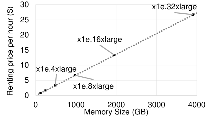
While many parallel multicore algorithms are work-efficient and have low 0pt, the auxiliary memory required by the algorithms can prevent larger inputs from being processed. Purchasing or renting machines multicore machines with larger memory capacities is an option, but for large enough machines, the cost increases roughly linearly with the memory capacity, as shown in Figure 1. Furthermore, additional energy costs need to be paid for machines that are owned, and the energy cost increases proportionally with the memory capacity. Therefore, designing parallel in-place (PIP) algorithms, which use auxiliary space that is sublinear (or even polylogarithmic) in the input size, can lead to considerable savings. In addition, in-place algorithms can also reduce the number of cache misses and page faults due to their lower memory footprint, which in turn can improve overall performance, especially in parallel algorithms where memory bandwidth and/or latency is a scalability bottleneck.
There has been recent work studying theoretically-efficient and practical parallel in-place algorithms for sample sort (axtmann2017place, ), radix sort (obeya2019theoretically, ), partition (kuszmaul2020cache, ), and constructing implicit search tree layouts (berney2018beyond, ). These PIP algorithms achieve better performance than previous algorithms in almost all cases. While these algorithms are insightful and motivate the PIP setting, they are algorithms designed for specific problems and have different notions of what “in-place” means in the parallel setting. In this paper, we generalize the ideas in previous work into two models, which we refer to as the strong PIP model and the relaxed PIP model. At a high level, the relaxed PIP model provides similar properties to the classic in-place PRAM model, and the strong PIP model puts further restrictions on memory allocation that allows PIP algorithms to simultaneously achieve small auxiliary space and low span. We provide more details on these models in Section 3.
The main contribution of this paper is a collection of new PIP algorithms in the two models, which include algorithms for solving scan, merge, filter, partition, sorting, random permutation, list contraction, tree contraction, and several graph problems (connectivity, biconnectivity, and minimum spanning forest). The results are summarized in Table 1, and discussed in more detail in Sections 4–6. Some of the algorithms are known, and we summarize them in this paper. The rest are new to the best of our knowledge, and we distinguish them by presenting our results in theorems and corollaries.
| Model | Problems | Work-efficient | |
| Strong PIP Model | Permuting tree layout | ✓ | (berney2018beyond, ) |
| Reduce, rotating | ✓ | ||
| Scan (prefix sum) | ✓ | * | |
| Filter, partition, quicksort | |||
| Merging, mergesort | |||
| Set operations | ✓ | (BlellochFS16, ) | |
| Relaxed PIP Model | Random permutation | ✓ | * |
| List and tree contraction | ✓ | * | |
| Merging, mergesort | ✓ | * | |
| Filter, partition, quicksort | ✓ | ||
| (Bi)Connectivity | * | ||
| Minimum spanning forest | * |
The algorithmic highlight in this paper is the Decomposable Property defined in Section 4. The high-level idea is to iteratively reduce a problem to a subproblem of sufficiently smaller size, where the the reduction can be performed using a non-in-place algorithm for the same problem. If we can perform the reduction efficiently, then this leads to an efficient algorithm in the relaxed PIP model. This means that we can convert any existing non-in-place but highly-optimized parallel algorithm to an efficient PIP algorithm. We show many examples of this approach in this paper, including algorithms for random permutation, list contraction, tree contraction, merging, and mergesort. We have also designed other PIP algorithms without using the Decomposable Property, including algorithms for scan, filter, and various graph problems.
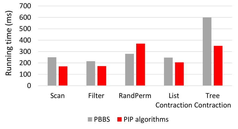
We implement five of our in-place algorithms, and compare them to the optimized non-in-place implementations in the Problem Based Benchmark Suite (PBBS) (shun2012brief, ). The running time comparisons for certain input sizes are shown in Figure 2 and we provide more details in Section 7. We show that in addition to lower space usage, our in-place algorithms can have competitive or even better performance compared to their non-in-place counterparts due to their smaller memory footprint, indicating that the theory for PIP algorithms developed in this paper can lead to practical outcomes. Our implementations are publicly-available at https://github.com/ucrparlay/PIP-algorithms.
2. Preliminaries
Work-Span Model. In this paper, we use the classic work-0pt model for fork-join parallelism with binary forking for analyzing parallel algorithms (CLRS, ; blelloch2020optimal, ). Unlike machine-based cost models such as the PRAM model (JaJa92, ), this model is a language-based model, and we will justify the use of this model in Section 3. In this model, we assume that we have a set of threads that have access to a shared memory. Each thread supports the same operations as in the sequential RAM model, but also has a fork instruction that forks two new child threads. When a thread performs a fork, the two child threads all start by running the next instruction, and the original thread is suspended until all of its children terminate. A computation starts with a single root thread and finishes when that root thread finishes. The work of an algorithm is the total number of instructions and the 0pt (depth) is the length of the longest sequence of dependent instructions in the computation. A thread can allocate a fixed size of memory that is either shared by all threads (referred to as “heap-allocated” memory), or private to this thread and other threads that it forks (referred to as “stack-allocated” memory). The latter case requires freeing the memory allocated after a fork and before the corresponding join. A randomized work-stealing scheduler, which is widely used in real-world parallel languages such as Cilk, TBB, and X10, can execute an algorithm with work and 0pt in time whp111We say with high probability (whp) to indicate with probability at least for , where is the input size. on processors (BL98, ; ABP01, ).
In this paper, we also analyze the auxiliary space used, and we measure space in units of words.
Work-Efficient and Low-Span Parallel Algorithms. The goal of designing a parallel algorithm is to achieve work-efficiency and low span. Work-efficiency means that the algorithm asymptotically uses no more work than the best (sequential) algorithm for the problem. Low span means that the longest sequence of dependent operations has polylogarithmic length. Achieving low span can lead to practical benefits. For instance, the number of steals in a work-stealing scheduler can be bounded by , which is proportional to the number of extra cache misses due to parallelism (Acar02, ; blelloch2010low, ). Low span also leads to fewer rounds of global synchronization, which can lead to significant performance improvements on modern architectures.
The “busy-leaves” property. When using the Cilk work-stealing scheduler, a fork-join program that uses words of space in a stack-allocated fashion when run on one processor will use words of space when run on processors (BL98, ). This is a consequence of the “busy-leaves” property of the work-stealing scheduler.
Problem definitions. Here we define the problems that are used in multiple places in this paper. Other problems are defined in their respective sections. Consider a sequence , an associative binary operator , and an identity element . Reduce returns . Scan (short for an exclusive scan) returns , in addition to the sum of all elements. An inclusive scan returns . Filter takes an array and a predicate function , and returns a new array containing for which is true. Partition is similar to filter, but in addition to placing the elements where is true at the beginning of the array, elements for which is false are placed at the end of the array. We say that a filter or partition is stable if the elements in the output are in the same order as they appear in .
3. Models for Parallel In-Place Algorithms
In the past, PIP algorithms have been designed based the in-place PRAM model (guan1991time, ; langston1993time, ; zheng1999efficient, ; guan1992parallel, ; huang1989stable, ; pietracaprina2015space, ). However, this model and the PRAM model itself have some limitations, which we describe in Section 3.3. Hence, recent work on PIP algorithms (axtmann2017place, ; obeya2019theoretically, ; kuszmaul2020cache, ; berney2018beyond, ) incorporate the PIP setting in the newer work-span model, although they use different notions of “in-place” for the algorithms. In this paper, we generalize the ideas into two models, which we refer to as the strong PIP model and the relaxed PIP model. At a high level, the relaxed PIP model provides similar properties as the in-place PRAM model, and the strong PIP model puts further restrictions on memory allocation that enables PIP algorithms to achieve small auxiliary space and low span simultaneously. Based on our model definitions, algorithms in (kuszmaul2020cache, ; berney2018beyond, ) can be mapped to the strong PIP model, and algorithms in (axtmann2017place, ; obeya2019theoretically, ) can be mapped to the relaxed PIP model. In this section, we will first define these two models, and then discuss their relationship to existing PIP models.
3.1. The Strong PIP Model
We start by defining the strong PIP model based on the work-span model for fork-join parallelism.
Definition 3.1 (Strong PIP model and algorithms).
The strong PIP model assumes a fork-join computation only using -word auxiliary space in a stack-allocated fashion for an input size of when run sequentially (with no auxiliary heap-allocated space). We say that an algorithm is strong PIP if it runs in the strong PIP model and has polylogarithmic 0pt.
For a PIP algorithm in the strong PIP model, the Cilk work-stealing scheduler can bound the total auxiliary space to be words, where is the number of processors (BL98, ). All strong PIP algorithms presented in this paper, as well as existing ones (berney2018beyond, ; kuszmaul2020cache, ), only use -word stack-allocated auxiliary space sequentially. We say a strong PIP algorithm is optimal if its work and 0pt bounds match the best non-in-place counterpart.
3.2. The Relaxed PIP Model
Many existing PIP algorithms (guan1991time, ; langston1993time, ; zheng1999efficient, ; guan1992parallel, ; huang1989stable, ; pietracaprina2015space, ; axtmann2017place, ; obeya2019theoretically, ) exhibit a tradeoff between additional space and 0pt , such that .222We use to hide polylogarithmic factors. We capture these algorithms in our relaxed PIP model, and refer to these algorithms as relaxed PIP algorithms.
Definition 3.2 (Relaxed PIP model and algorithms).
The relaxed PIP model assumes a fork-join computation using -word stack-allocated space sequentially and shared (heap-allocated) auxiliary space for an input of size and some constant . We say that an algorithm is relaxed PIP if it runs in the relaxed PIP model and has 0pt for all values of .
The Cilk work-stealing scheduler can bound the total auxiliary space of relaxed PIP algorithms to be on processors. For brevity, we refer to the auxiliary space in future references to the relaxed PIP model as just the heap-allocated space. Algorithms in the relaxed PIP model allow sublinear auxiliary space, which is less restrictive than in the strong PIP model. This provides more flexibility in algorithm design, while still being useful in practice as relaxed PIP algorithms still use less space than their non-in-place counterparts. In the next section, we introduce a general property, which allows any existing parallel algorithm with polylogarithmic span that satisfies the property to be easily converted into a relaxed PIP algorithm.
3.3. Relationship to Previous Models
PIP algorithms have been analyzed in the in-place PRAM model for decades. Recent work (axtmann2017place, ; obeya2019theoretically, ; kuszmaul2020cache, ; berney2018beyond, ) has designed in-place algorithms into the work-span model, but they only provide algorithms for specific problems rather than focusing on the general parallel in-place setting. In this paper, we formally define the parallel in-place models, and justify the models by discussing the limitations of the previous in-place PRAM, and how our new models overcome it.
The in-place PRAM. Most existing parallel in-place algorithms have been designed in the in-place PRAM (guan1991time, ; langston1993time, ; zheng1999efficient, ; guan1992parallel, ; huang1989stable, ; pietracaprina2015space, ). The PRAM has processors that are fully synchronized between steps, and the running time of an algorithm is the maximum number of steps used by any processor. In this model, the auxiliary space is the sum of the total space used across all processors. As pointed out by Berney et al. (berney2018beyond, ), each processor on a PRAM requires (usually ) auxiliary space to do anything useful (e.g., storing the program counter and using registers). This indicates that if the total auxiliary space for all processors is bounded to be small, then the parallelism is also bounded by . This is because even if we have an infinite number of processors, no more than of them can do useful work simultaneously. The overall PRAM time is , where is the overall work in the algorithm. Hence, in the PRAM setting, an algorithm can only achieve high parallelism when is asymptotically close to . This has been described by Langston et al. (langston1993time, ; zheng1999efficient, ; guan1992parallel, ; huang1989stable, ) as the time-space tradeoff in the PRAM—if the input size is , then the product of auxiliary space and PRAM time is , and an algorithm is optimal on a PRAM when . This limitation arises because the analysis of parallelism and auxiliary space are intertwined in the in-place PRAM.
Decoupling the analysis between parallelism and auxiliary space. Parallel algorithms with low span have many practical benefits even for small processor counts, due to lower scheduling overhead and improved cache locality, as discussed in Section 2. However, low span cannot be achieved in the in-place PRAM unless we use nearly linear auxiliary space. Our goal is to decouple the analysis of parallelism from the restriction of auxiliary space. In both the strong PIP and relaxed PIP models, the auxiliary space in measured in the sequential setting, whereas the span is analyzed based on the fork-join computation graph. This decouples the space analysis from the span analysis. Furthermore, in the strong PIP model, low span and small auxiliary space can be achieved simultaneously.
To achieve the decoupling, we use the separation of the private “stack-allocated” memory from the shared “heap-allocated” memory in work-span model. The heap-allocated memory is what we usually refer to as the shared memory, and is independent of the number of processors. The stack-allocated memory is per processor, and the “busy-leaves” property guarantees that the overall space usage of a program is when it is run on processors, where is the amount of stack-allocated memory when running the algorithm sequentially. Since is usually modest in practice, if the stack-allocated memory is small (e.g., ), then the auxiliary space size will be negligible on modern machines. As a result, the abstraction of the stack-allocated memory separates the per-processor need from the shared resource, and overcomes the limitation of the in-place PRAM by dynamically mapping the algorithm on a machine with processors, with the auxiliary space guarantee.
In addition to the advantages discussed above, the work-span model simplifies parallel algorithm design and analysis, and algorithm designers do not need to worry about low-level details related to hardware such as memory allocation, caching, and load balancing. Recent papers (berney2018beyond, ; kuszmaul2020cache, ; obeya2019theoretically, ) have made a similar observation on the limitation of the in-place PRAM model, and analyzed the in-place algorithms using the work-span model. In this paper, we explicitly formalize this discussion and define the two PIP models based on the work-span model.
Other practical considerations. Here we describe additional benefits to use the new PIP models based on the work-span model. Modern parallel programming languages, such as Cilk, OpenMP, TBB, and X10, directly support algorithms designed for the work-span model using fork-join parallelism, with efficient runtime schedulers. In contrast to the PRAM, in which computations have many synchronization points, computations in the work-span model can be highly asynchronous. This is a practical advantage due to the high synchronization overheads on modern hardware (blelloch2020optimal, ). Furthermore, the PIP algorithms in this paper based on our new models have additional guarantees with respect to multiprogrammed environments (ABP01, ), cache complexity (Acar02, ; BlellochFinemanGibbonsEtAl2011, ; blelloch2010low, ), write-efficiency (BBFGGMS16, ; blelloch2015sorting, ; blelloch2016efficient, ), and resource-obliviousness (Cole2017, ).
4. Decomposable Property
Designing strong PIP algorithms is generally challenging (we present several in Section 5, but if we relax the auxiliary space to sublinear (the relaxed PIP model), then we believe that PIP algorithms can be designed for many more problems. In this section, we introduce the Decomposable Property, which enables any existing parallel algorithm that satisfies the property to be converted into a relaxed PIP algorithm. If the existing parallel algorithm is work-efficient, then the corresponding relaxed PIP algorithm will also be work-efficient.
Theorem 4.1 (Decomposable Property).
Consider a problem with input size and a parallel algorithm to solve it with work . Let . If the problem can be reduced to a subproblem of size using work and space for some , and polylogarithmic 0pt , then there is a relaxed PIP algorithm for this problem with work, span, and auxiliary space.
Proof.
We iteratively reduce the problem size by (this size remains the same throughout the algorithm), and each round takes work and space. Since , this means is asymptotically larger than , and we can reduce the problem size by at least one on each round. By applying this reduction for rounds, we have a relaxed PIP algorithm with work and 0pt, using auxiliary space. ∎
The high-level idea of the Decomposable Property is that, for a problem of size , if we can reduce the problem size to using work proportional to , then we can control the additional space by varying the size of to fit in the auxiliary space. This provides theoretically-efficient relaxed PIP algorithms for parallel algorithms that satisfy this property. On the practical side, we observe that this reduction step usually corresponds to solving a subproblem that is the same as the original problem but with a smaller size. Hence, we can use the best existing non-in-place algorithms for this step. We show in Section 7 that the performance of our relaxed PIP algorithms using this approach is competitive or faster than their non-in-place counterparts. In the rest of this section, we introduce some algorithms that satisfy the Decomposable Property.
4.1. Random Permutation
Generating random permutations in parallel is a useful subroutine in many parallel algorithms. Many parallel algorithms (e.g., randomized incremental algorithms) require randomly permuting the input elements to achieve strong theoretical guarantees. The sequential Knuth (Knuth69, ; Durstenfeld1964, ) shuffle algorithm, shown below, has linear work, where is an integer uniformly drawn from , and is the array to be permuted.
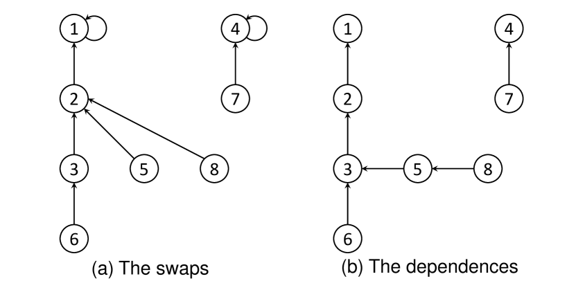
Recent work (shun2015sequential, ) has shown that this sequential iterative algorithm is readily parallel. The pseudocode of this parallel algorithm is shown in Algorithm 1, and is both theoretically and practically efficient. The key idea is to allow multiple swaps to be performed in parallel as long as the sets of source and destination locations of the swaps are disjoint. We illustrate the dependence structure on an example in Figure 3. Given an input array , in Figure 3(a) we create a node for each index, and an edge from the node to the node corresponding to its swap destination. In this example, we can swap locations 6 and 3, 8 and 2, and 7 and 4 simultaneously in the first step since these three swaps do not interfere with each other. To resolve the case where multiple nodes point to the same swap destination, we chain these nodes together, as shown in Figure 3(b). We also remove self-loops. In Algorithm 1, each unfinished swap writes to an auxiliary array using a to reserve both its source and destination locations (Lines 1–1). We assume that takes work, and in practice, it can be implemented using a compare-and-swap loop (shun13reducing, ). We then perform the actual swaps in parallel for the swaps that successfully reserve both of its locations (Line 1). The rest of the swaps will be packed and will try again in the next step. Shun et al. show that Algorithm 1 finishes in rounds whp (shun2015sequential, ). The work and 0pt can be shown to be in expectation and whp, respectively (shun2015sequential, ; blelloch2020optimal, ).
We now show that the random permutation algorithm above satisfies the Decomposable Property. The property for the sequential Knuth shuffle is easy to see—after applying the first swaps, which we refer to as one round, the problem reduces to a subproblem of size , which can be solved using the same algorithm. We note that for any swaps, up to locations will be accessed in the and arrays (, , and for each swap source ). We can use a parallel hash table to store these values using space. When the load factor of the hash table is no more than one-half, then each update or query requires expected work and work whp (knuth1963notes, ; shun2014phase, ). To guarantee that our algorithm has the same bounds as proved in (shun2015sequential, ; blelloch2020optimal, ), we always work on the first unfinished swaps based on the sequential order. The longest dependence length among the first swaps in a phase is bounded by whp since it cannot be longer than the overall dependence length for all swaps, which is bounded by whp. The overall 0pt in a phase is , where the additional factor of due to hash table insertions and queries. The entire algorithm finishes after rounds and is work-efficient. By applying Theorem 4.1, we obtain the following theorem.
Theorem 4.2.
There is a relaxed PIP algorithm for random permutation using expected work, 0pt whp, and auxiliary space for .
Constant-dimension linear programming and smallest enclosing disks. Based on the relaxed PIP algorithm for random permutation, it is straightforward to design relaxed PIP algorithms for constant-dimension linear programming and smallest enclosing disks using randomized incremental construction (seidel1993backwards, ; blelloch2016parallelism, ). The randomized algorithms after randomly permuting the input elements take expected work and span and auxiliary space whp, where is the dimension (blelloch2016parallelism, ), by using the in-place reduce algorithm that will be discussed in Section 5. By using the relaxed PIP random permutation algorithm, we can obtain parallel in-place algorithms for constant-dimension linear programming and smallest enclosing disks in expected work and 0pt whp, using auxiliary space.
4.2. List Contraction and Tree Contraction
List ranking (Reid-Miller93, ; KarpR90, ; JaJa92, ) is one of the most important problems in the study of parallel algorithms. The problem takes as input a set of linked lists, and returns for each element its position in its list. List contraction is used to contract a linked list into a single node, and is used as a subroutine in list ranking.
We now discuss the Decomposable Property of list contraction. The order of contracting elements does not matter as long as all elements are eventually contracted. Therefore, similar to random permutation, we can process elements in a round, and apply existing parallel list contraction algorithms (KarpR90, ; JaJa92, ) to contract these elements. To show an example, we discuss Shun et al.’s non-in-place list contraction algorithm (shun2015sequential, ) and how to turn it into a relaxed PIP algorithm. This is also the algorithm that we implemented in this paper.
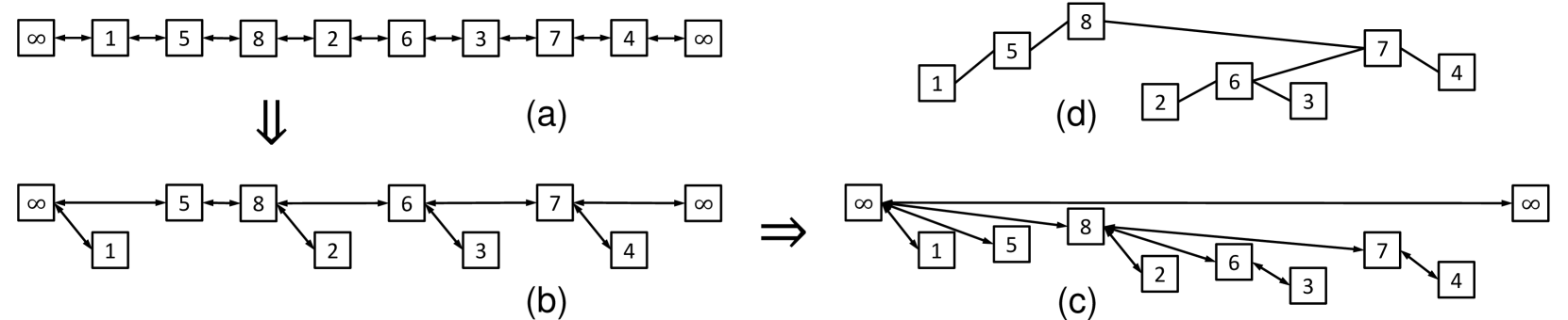
The pseudocode and the high-level idea of this algorithm is given in Algorithm 2. A careful implementation of this algorithm takes worst-case linear work and span whp (shun2015sequential, ; blelloch2020optimal, ). This algorithm assigns a random priority to each list element (Figure 4(a)), contracts all elements that have priority lower than both of its neighbors’ priorities (Figure 4(b)), packs the leftover elements, and iterates until the list is empty. The number of rounds of this algorithm is the length of the longest dependence among the nodes, which is whp (shun2015sequential, ). Figure 4(d) shows the dependences in the example (a node depends on all of its descendants in the tree shown)—here the algorithm finishes in 4 rounds (the height of the tree).
As discussed, the order of the contraction does not matter. Hence, for a problem of size , we can work on elements and contract them using this algorithm, which requires work, span whp (no more than the span for elements), and space. Then the problem reduces to a subproblem of size . We can iteratively apply this for rounds, which yields a relaxed PIP algorithm for list contraction.
After the elements are spliced out, list contraction algorithm generates a tree, and the tree for the example in Figure 4(a) is shown in Figure 4(c). The remaining work in list ranking after list contraction is referred to as “reconstruction” (JaJa92, ), which distributes the values down the tree. Therefore, once we obtain this tree structure, the classic algorithms (JaJa92, ; Reif1993, ) for reconstruction take worst-case linear work and span whp. Representing the tree only requires pointers, which fit into the pointers in the input linked list if we are allowed to overwrite the input. For our new relaxed PIP algorithm, we can store the tree pointers in each round by overwriting the pointers of the elements being processed in the current round. After we recursively solve the smaller subproblem, we can use the classic reconstruction algorithm for the elements in the current round, which takes worst-case linear work and logarithmic span whp. In total, the reconstruction step has the same work, span, and auxiliary space bounds as list contraction.
Tree contraction is a generalization of list contraction and has many applications in parallel tree and graph algorithms (Reid-Miller93, ; JaJa92, ; MillerReif1985, ; shun2015sequential, ). Here we will assume that we are contracting rooted binary trees in which every internal node has exactly two children. As in list contraction, the ordering of contracted tree nodes does not matter as long as a parent-child pair is not contracted in the same round. For a problem of size , we can work on tree nodes each round and contract them using existing tree contraction algorithms, and repeat for rounds. Therefore, the Decomposable Property is satisfied for tree contraction. We can convert the parallel tree contraction algorithm of Shun et al. (shun2015sequential, ; blelloch2020optimal, ) that is not in-place, but theoretically and practically efficient, to a relaxed PIP algorithm that requires expected work and 0pt whp per round, and space.
We obtain the following theorem for list contraction and tree contraction.
Theorem 4.3.
There are relaxed PIP algorithms for list contraction and tree contraction that take work, span whp, and auxiliary space for .
4.3. Merging and Mergesort
Merging two sorted arrays of size and (stored consecutively in an array of size ) is another canonical primitive in parallel algorithm design. We assume without loss of generality that . Parallel in-place merging algorithms have been studied for the PRAM model (guan1991time, ), using work, span, and auxiliary space when mapped to the relaxed PIP model. However, this algorithm is quite complicated and unlikely to be practical. By using the Decomposable Property, we can design a much simpler algorithm based on any existing textbook parallel non-in-place merging algorithm, combined with some features of the sequential in-place merging algorithm (huang1988practical, ). The key idea in (huang1988practical, ) for in-place merging is to split both input arrays into chunks of size , and sort the chunks based on the last element of each chunk. Then, the algorithm merges the first remaining chunk from each of the two input arrays, and when one chunk is used up, the algorithm replaces it with the next chunk in the corresponding array.
To obtain a relaxed PIP algorithm, we set the chunk size to , so that we can process two chunks using auxiliary space. With this space bound, we can use a non-in-place merging algorithm to output the smallest elements and repeat for rounds.
The first step of our algorithm is the same as (huang1988practical, ), which sorts the chunks based on only their last elements, and moves each chunk to their final destination in parallel by using the auxiliary space as a buffer. Sorting all of the chunks takes span. Then, in the merging phase, we move the first chunk from each array to the auxiliary space, use any existing parallel merging algorithm to merge them, until we either run out of the elements in one chunk, at which point we load the next chunk of the corresponding array to the auxiliary space, or until we gather a full chunk of merged elements, at which point we flush it back to the original array and empty the buffer. At any time, there can be at most three chunks in the auxiliary space—two chunks from the input arrays and one chunk for the merged output, and so the required auxiliary space is . We can use any existing non-in-place parallel algorithm (blelloch2018introduction, ; JaJa92, ) to perform the merge in the auxiliary space, which takes linear work and logarithmic 0pt. Such calls to merge in the algorithm can happen at most times— times after loading new chunks to the auxiliary space and times after the output chunk is full and is flushed. Each merge takes work linear in the output size, and span. The overall work is therefore , and the 0pt is . This gives the following theorem.
Theorem 4.4.
Merging two sorted arrays of size and (where ) stored consecutively in memory takes work, span, and auxiliary space for .
When , the auxiliary space is insufficient for sorting all chunks at the beginning, and so we sort chunks at a time until all chunks have been processed. As done in (huang1988practical, ), we use dual binary search to find the smallest chunks to merge, and repeat our above algorithm for rounds. This will not affect the cost bounds.
With the relaxed PIP merging algorithm, we can obtain a relaxed PIP mergesort algorithm with work, auxiliary space, and span.
4.4. Filter, Unstable Partition, and Quicksort
It is easy to see that we can work on a prefix of the filter problem of size using linear work and logarithmic 0pt, and repeat for rounds. The only additional work is to move the unfiltered elements to the beginning of the array, which can be done in linear work and span for each prefix. This gives a relaxed PIP algorithm for filter that takes work, span, and auxiliary space. We can implement partition similarly, and when moving the unfiltered elements to the beginning, we swap the elements so that at the end of the algorithm, the filtered elements are moved to the end of the array. This algorithm has the same cost as filter, although the partition result is not stable. With the relaxed PIP partition algorithm, we can obtain a relaxed PIP algorithm for (unstable) quicksort that takes expected work and span whp, and auxiliary space.
5. Strong PIP Algorithms
The strong PIP model is restrictive because of the polylogarithmic auxiliary space requirement. To date, only a few non-trivial and work-efficient strong PIP algorithms have been proposed: reducing and rotating an array, which are trivial, certain fixed permutations (berney2018beyond, ), and two-way partitioning (kuszmaul2020cache, ). In this section, we review existing strong PIP algorithms for reduce and rotation, and present new algorithms for scan (prefix sum), filter, merging, and sorting.
5.1. Existing Algorithms
Reduce. The classic divide-and-conquer algorithm for reduce is already strong PIP. It is implemented by dividing the input array by two equal sized subarrays, recursively solving the two subproblems in parallel, and finally summing together the partial sums from the two subproblems. This algorithm requires sequential stack space, work and span, and so it is an optimal strong PIP algorithm.
Rotating an array. Given an array and an offset , the output is a rotated array . This can be implemented by first reversing , then reversing , and finally reversing the entire array. Reversing can be implemented with a parallel loop, which requires stack space when run serially. This algorithm requires work and span, and is therefore an optimal strong PIP algorithm.
5.2. Scan
Scan (prefix sum) is probably the most fundamental algorithmic primitive in parallel algorithm design. Here we assume is (addition) for simplicity, but the results in this section also apply to other associative binary operators. Non-in-place implementations of scan have been designed since the last century, and the work-efficient version is generally referred to as the Blelloch scan (blelloch1990pre, ). The Blelloch scan contains two phases. The first phase is referred to as the “up-sweep”, which partitions the array into two halves, computes the sum recursively for each half, then uses the prefix sums for each half to calculate the prefix sums for the entire sequence, and finally stores this result in auxiliary space. Then the algorithm applies a “down-sweep” phase, which propagates the sums from the first phase down to each element recursively—for a subproblem with a prefix sum of ( for the subproblem corresponding to the whole sequence), we recursively solve the left half with prefix sum , and the right half with prefix sum plus the sum of the left half, in parallel. This algorithm takes work and 0pt, but unfortunately, it requires linear auxiliary space to store all of the partial sums.
Making existing approaches in-place. We first discuss a solution to make the Blelloch scan in-place. We partition the array into two equal-sized halves, recursively solve each half, and apply a parallel for-loop to add the sum of the left half to every element in the right half. Directly applying this algorithm leads to work, since the recursion tree has levels, and on each level we need to perform additions, which takes work and span. We can reduce the work overhead by stopping the recursion when we reach a subproblem of size no more than (these subproblems constitute the base cases), and apply a sequential in-place scan for these subproblems, and store the partial sums in the last elements of the subproblem arrays. We then run scan on the sums of the base cases using the aforementioned algorithm. This scan takes work and computes the prefix sum before the beginning of each base case. Lastly, we add this prefix sum to the elements in each base case subproblem to obtain the final result for scan. This algorithm uses work, 0pt, and auxiliary space, which is the recursion depth.
Another approach is to use the Brent-Kung adder (brent1982regular, ), which is a circuit to solve the scan problem with 0pt, gates, and area. We can change the circuit to an algorithm that contains parallel for-loops and each for-loop simulates the gates at one level. The work of this algorithm is linear, which is the same as the number of gates, and the 0pt is — parallel for-loops each taking span for forking the tasks. The output of the original circuit is an inclusive scan (i.e., the output is ). The circuit can be modified to compute the exclusive scan in the same bounds. In conclusion, we can make the the existing approaches in-place, but their span would not be optimal.
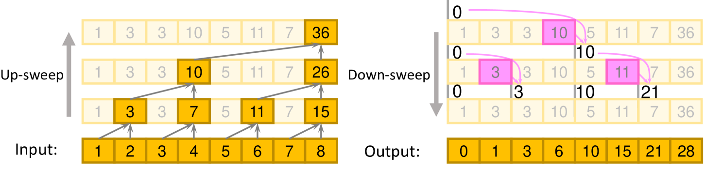
A new optimal strong PIP algorithm. Our new strong PIP algorithm is almost as simple as the non-in-place Blelloch scan, and has the same work and span bounds. The new algorithm as shown in Algorithm 3, and illustrated in Figure 5. In the pseudocode, we assume when it is referenced, but the algorithm does not actually need to store this. The new strong PIP algorithm also contains two phases: the up-sweep and the down-sweep phases, both of which are recursive. The key insight in our new algorithm is to maintain all of the intermediate results in the input array of elements, and use stack space in the down-sweep phase to pass down the partial sums. For each recursive subproblem corresponding to a subarray from index to , we partition it into two halves, to and to , where . In the up-sweep phase, we first recursively solve the two subproblems, and then add the value at index to the value at index . These additions are shown as arrows on the left side of Figure 5. In the down-sweep phase, we keep the prefix sum of each subproblem. Similar to the Blelloch scan, we compute the prefix sum of the right subproblem by adding the sum of the left subproblem to the current prefix sum. In our algorithm, the sum of the left subproblem is stored at . Both recursions stop when , and at the end of the down-sweep, we obtain the exclusive scan result. The down-sweep process and its output on an example are shown on the right side of Figure 5.
Correctness and efficiency. The correctness and efficiency of this algorithm is based on the following observation. In the down-sweep phase, the value of in any recursive call is not being used (except for the root where is the total sum). Hence, in our algorithm, we reuse the space for to store the sum for the next level. The reduction tree (left side of Figure 5) has nodes: nodes for the input and internal nodes storing the partial sums. We note that in the down-sweep phase, only the sums of the left subproblems are used, and there are of them. They are stored in by the end of up-sweep, while stores the total sum. With all of these values, we can run the down-sweep phase in the same way as in the Blelloch scan. The partial sums stored in are passed to the output by the argument in the down-sweep function call, which is stored in the stack space. Hence, the new strong PIP scan algorithm uses work, 0pt, and sequential auxiliary stack space, and is therefore an optimal strong PIP algorithm.
Theorem 5.1.
The new strong PIP scan algorithm is optimal, using work, 0pt, and sequential auxiliary space.
5.3. Other Strong PIP Algorithms
Filter, unstable partition, and quicksort. Consider a -way divide-and-conquer algorithm for filter, where we partition the array into chunks of equal size, filter each chunk, and pack the unfiltered results together. For one level of recursion, this takes linear work and span if chunks are processed one at a time, but within each chunk we move the elements in parallel. This algorithm only requires a constant amount of extra space to store pointers. The number of levels of recursion is , and so the overall work is , and the overall span is . Similar to Section 4.4, we can use this filter algorithm to implement an unstable partition algorithm, with the same cost bounds. In theory, we can plug in any constant for , which gives a strong PIP algorithm with 0pt and auxiliary space, although it is not work-efficient. Alternatively, we can achieve work-efficiency by setting . This does not achieve polylogarithmic 0pt, but has good performance in practice. We implement this filter algorithm and present experimental results in Section 7.
We can obtain an unstable quicksort algorithm that applies the partition algorithm for levels of recursion whp. We note that Kuszmaul and Westover (kuszmaul2020cache, ) recently developed a work-efficient strong PIP algorithm for partition, which gives a work-efficient and polylogarithmic-span quicksort algorithm.
Merging and mergesort. We again consider merging two sorted arrays of size and , which are stored consecutively in an array of size . Again, we can use a two-way divide-and-conquer approach, where we use a dual binary search to find the median among all elements, and in parallel swap the out-of-place elements in two arrays. This swap can be implemented by the strong PIP algorithm for array rotation, discussed in Section 5.1. Then, we recursively run merging on the two subproblems, each of size . The subproblem size shrinks by a factor of 2 on each level of recursion, and so the recursion depth is bounded by . The work to swap the elements at each level is , and so the overall work is . The span and auxiliary space is , which is proportional to the recursion depth. This gives a strong PIP algorithm for merging. A strong PIP mergesort algorithm can be obtained by plugging in this merging algorithm, although it is not work-efficient.
Set operations. We now consider computing the union, intersection, and difference of two ordered sets of size and . If the two sets are given in a binary tree format, then existing algorithms for these operations (BlellochFS16, ; pam, ) are already strong PIP, work-optimal ( work), and have span. We now describe how to implement these operations if the sets are given in arrays stored contiguously in memory. For union, we can first use the merging algorithm described above, and then the filter algorithm described above to remove duplicates. Therefore, computing the union on arrays is strong PIP. For intersection and difference, we can run binary searches to find each element in the smaller set inside the larger set, and then apply the filter algorithm described above to obtain the output, which takes work. The resulting algorithms are not work-efficient, since our strong PIP merging and filter are not work-efficient.
6. Relaxed PIP Graph Algorithms
In this section, we introduce new relaxed PIP algorithms for graph connectivity, biconnectivity, and minimum spanning forest.
Connectivity and Biconnectivity. The standard output size for graph connectivity and biconnectivity is and , respectively. Recent work by Ben-David et al. (bendavid2017implicit, ) introduces a compressed scheme for storing graph connectivity information. For any , it requires output size with an expected query work for connectivity and expected query work for biconnectivity. Constructing such a compressed (bi)connectivity oracle takes expected work and span whp. By setting , we have have the following theorem.
Theorem 6.1.
A (bi)connectivity oracle can be constructed using auxiliary space, expected work, and span whp for . A connectivity query can be answered in expected work, and a biconnectivity query can be answered in expected work.
The high-level idea in the algorithms is to select a subset of the vertices as the “centers” and only keep information for these center vertices. Each vertex has a probability of being selected as a center. This is referred to as the implicit decomposition of the graph. For a query to a non-center vertex , we apply a breadth-first search from to the first center , which takes expected work (bendavid2017implicit, ). For connectivity, ’s label is the same as ’s label. It is also possible that a search does not reach any center, but Ben-David et al. (bendavid2017implicit, ) show that the expected size of a connected component without a center vertex is small ( in expectation), and so the cost to traverse all vertices in such a component is also in expectation. For biconnectivity, an additional step of local analysis is required to obtain the output for from , which requires expected work.
Theorem 6.1 gives algorithms that are almost relaxed PIP, other than having an extra factor of in the product of the space and span bounds. Alternatively, we can obtain new relaxed PIP connectivity and biconnectivity algorithms by using the minimum spanning forest algorithm that will be discussed next, at a cost of additional work.
Minimum Spanning Forest. The idea of implicit decomposition can be extended to the minimum spanning forest (MSF) problem. For simplicity, we assume that the graph is connected, but disconnected graphs can also be handled using an approach described by Ben-David et al. (bendavid2017implicit, ).
We note that the MSF is unique for a graph (assuming that ties are broken consistently). Therefore, for a query to vertex , instead of using a breadth-first search on all edges to find the center in connectivity, we need to search out to a center using only the MSF edges. This can be achieved by using a Prim-like search algorithm from . This increases the work by a factor of to compute the implicit decomposition of the graph and for the query cost (the queue will contains vertices on average for each search).
We can generate an implicit decomposition of the graph using a similar approach as for connectivity and biconnectivity. We then compute the MSF across the centers of the decomposition. The output size of this spanning forest is . To compute the MSF in parallel, we can use Borůvka’s algorithm. We start with every cluster being in its own component, and enumerate all edges for rounds until the entire graph is connected. On each round, we run Borůvka’s algorithm to find the minimum outgoing edges from each component. This takes work—we check all edges in a Borůvka’s round and each edge takes work to find the clusters of both of its endpoints. Similar to connectivity, each vertex only uses MST edges to reach the centers, and so the algorithm based on implicit decomposition is correct. By setting , the cost for each round is work and span. Since there are rounds, we obtain the following theorem.
Theorem 6.2.
Given a graph with vertices and edges, a data structure for minimum spanning forest can be computed in expected work, span whp, and auxiliary space. Querying if an edge is in the MSF takes work.
This MSF algorithm is relaxed PIP. Once we have the implicit spanning forest (the minimum-weight one in this case), we can use the same approaches mentioned above to get relaxed PIP algorithms for connectivity and biconnectivity. Compared to Theorem 6.1, the MSF-based algorithms require a factor of more work, but have lower span.
Related Work. Many researchers have studied the time-space tradeoff for the - connectivity problem, and the results lead to in-place algorithms for the problem (broder1994trading, ; feige1997spectrum, ; beame1998time, ; kosowski2013faster, ; edmonds1998time, ). However, the algorithms are based on random walks and are inherently sequential. Recent work by Chakraborty et al. (Chakraborty2018, ; Chakraborty2019, ; Chakraborty2020, ) has studied in-place algorithms for other graph problems, including graph search and connectivity, and it would be interesting to parallelize these algorithms in the future.
7. Implementations and Experiments
In the previous sections, we have designed parallel in-place algorithms with strong theoretical guarantees. Many of these algorithms are relatively simple, and in this section we describe how to implement these algorithms efficiently so that they can outperform or at least be competitive with their non-in-place counterparts, while using less space. We present implementations for five algorithms: scan, filter, random permutation, list contraction, and tree contraction. The implementations for the first two are fairly simple, and the last three are based on the deterministic reservations framework of Blelloch et al. (BlellochFinemanGibbonsEtAl2012, ).
7.1. Experimental Setup
We run all of our experiments on a 72-core Dell PowerEdge R930 (with two-way hyper-threading) with 42.4GHz Intel 18-core E7-8867 v4 Xeon processors (with a 4800MHz bus and 45MB L3 cache) and 1TB of main memory. We compile the code using the g++ compiler (version 5.4.1) with the -O3 flag, and use Cilk Plus for parallelism.
We compare our PIP algorithms to the non-in-place versions in the Problem Based Benchmark Suite (PBBS) (shun2012brief, ), which is a collection of highly-optimized parallel algorithms and implementations and widely used in benchmarking. The implementations of random permutation, list contraction, and tree contraction in PBBS are from (shun2015sequential, ).
Scan
Filter
List Contraction
Tree Contraction
7.2. Scan and Filter
For scan, we implement Algorithm 3 and switch to a sequential in-place scan when the subproblem size is less than 256. For filter, we implement the PIP algorithm from Section 5.3, but we keep the implementation work-efficient by setting the branching factor , and only apply one level of recursion. However, this increases the span to and has rounds of global synchronization (the chunks are processed one after another), which is a significant overhead. We use the following optimization to significantly reduce this overhead in practice. We move the elements from multiple consecutive chunks in parallel as long as the destination of the last chunk is before the original location of the first chunk. We apply a binary search in each round to find the maximum number of chunks that can be moved in parallel. If the unfiltered elements are distributed relatively evenly in the input and the output size is a constant fraction of the input, then the algorithm requires logarithmic rounds to finish.
We compare our PIP algorithms to the non-in-place versions in PBBS. The PBBS scan is the classic Blelloch scan implementation (Blelloch89, ) and the filter is similar to our implementation, but the output is stored in a separate array. In the PBBS filter, it first filters each -sized chunk in parallel while each chunk is processed sequentially, and then moves the remaining elements to a separate output array in parallel.
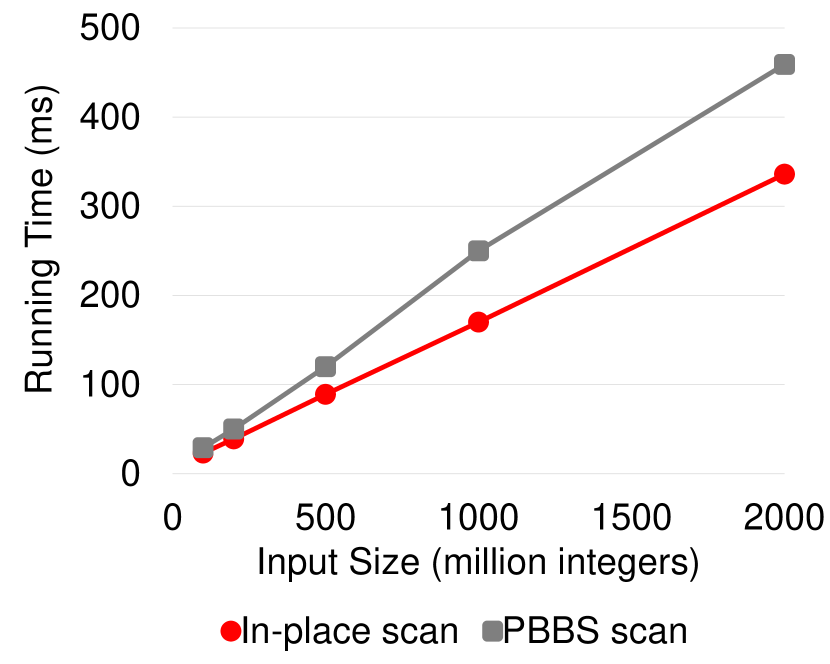
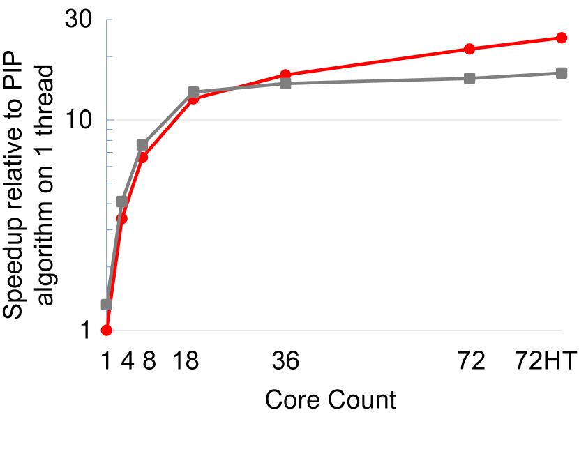
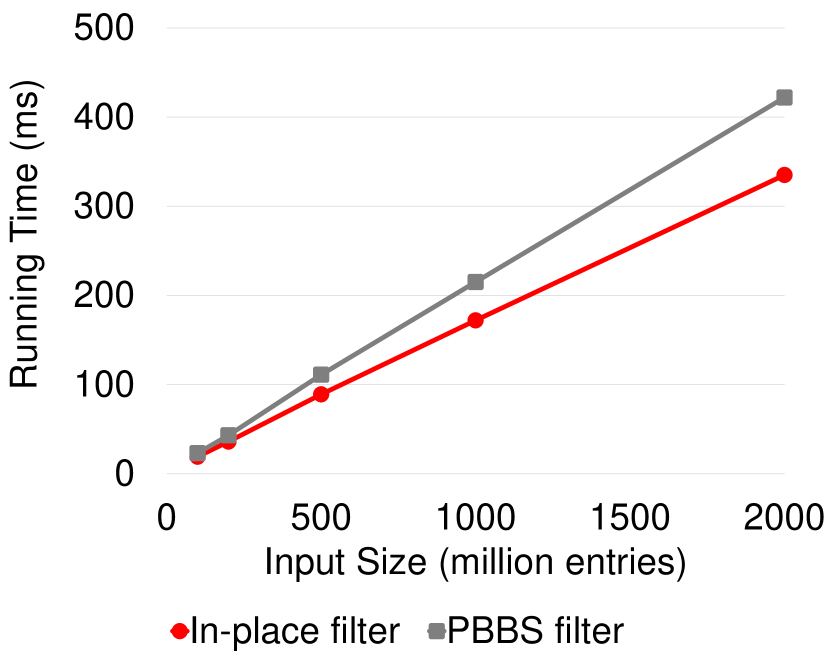
The running times and scalability (parallel speedup relative to the best algorithm on 1 thread, which was our PIP algorithm in all cases) for scan and filter on different input sizes are shown in Figure 6 and Tables 3–3. For filter, 50% of the input entries are kept in the output. Our in-place scan is 30–45% faster and our in-place filter is about 25–30% faster than their non-in-place counterparts due to having a smaller memory footprint. The speedups are also competitive or better than the non-in-place versions. For filter, the fraction of elements in the output affects the performance of both our algorithm and the PBBS algorithm. A larger output fraction increases the number of rounds for movement and global synchronization in the PIP filter algorithm. In Table 4, we vary the output fraction and show that our new algorithms range from about 2x faster (12.5% output) to having about the same performance (87.5% output).
| Input Size | Scan | Filter | ||
|---|---|---|---|---|
| (million) | PBBS | PIP | PBBS | PIP |
| 100 | 29 | 23 | 23 | 19 |
| 200 | 50 | 39 | 43 | 36 |
| 500 | 120 | 89 | 111 | 89 |
| 1000 | 250 | 170 | 215 | 172 |
| 2000 | 459 | 336 | 422 | 335 |
| Core | Scan | Filter | ||
|---|---|---|---|---|
| count | PBBS | PIP | PBBS | PIP |
| 1 | 3150 | 4170 | 2770 | 2150 |
| 4 | 1020 | 1230 | 861 | 701 |
| 8 | 548 | 630 | 524 | 393 |
| 18 | 308 | 331 | 301 | 244 |
| 36 | 280 | 255 | 254 | 191 |
| 72 | 265 | 192 | 222 | 179 |
| 72HT | 250 | 170 | 215 | 172 |
| Output fraction | 12.5% | 25% | 50% | 75% | 87.5% |
|---|---|---|---|---|---|
| PBBS filter | 189 | 202 | 215 | 234 | 252 |
| PIP filter | 94 | 118 | 172 | 212 | 254 |
This experiment indicates that using the PIP scan and filter algorithms can improve both the running time and memory usage over the non-in-place filter algorithm, and is preferable when the input can be overwritten. We note that ParlayLib (blelloch2020parlaylib, ), the latest version of PBBS, also includes the in-place versions of scan and filter, and we plan to compare with these in the future.
7.3. Deterministic Reservations
Implementing the PIP algorithms for random permutation, list contraction, and tree contraction is more challenging since they are more complicated than scan and filter. However, the Decomposable Property can greatly simplify the implementation of these algorithms, and we only need to design an efficient implementation working on a prefix of the problem and run it iteratively. Interestingly, the original implementations of these algorithms in (shun2015sequential, ) are based on a framework named as the deterministic reservations (BlellochFinemanGibbonsEtAl2012, ) that runs similarly in rounds, where each round processes a prefix of the remaining elements. We first briefly overview the framework of deterministic reservations, and then discuss how we can modify the original implementations to obtain new PIP algorithms for random permutation, list contraction, and tree contraction.
Deterministic reservations is a framework for iterates in a parallel algorithm to check if all of their dependencies have been satisfied through the use of shared data structures, and executing the ones that have been satisfied (BlellochFinemanGibbonsEtAl2012, ). Deterministic reservations proceeds in rounds, where on each round, each remaining iterate tries to execute. Iterates that fail to execute will be packed and processed again in the next round. To achieve good performance in practice, instead of processing all iterates on every round, the framework only works on a prefix of the remaining iterates (usually around 1–2% of the input iterates). This naturally meets our requirement for controlling the number of elements to process in the relaxed PIP algorithms. We provide more details on the framework in the appendix.
7.4. Random Permutation
We implement the PIP random permutation algorithm (Algorithm 1) based on deterministic reservations. We have four implementations (RP-Naïve, RP-Flat, RP-OneRes, and RP-Final), and each one improves upon the previous one. We compare our implementation to the code in PBBS library, and here we refer to it as RP-PBBS. More details on our implementations are provided in the appendix.
RP-PBBS runs in rounds, where each round processes a prefix of 2% of the total number of swaps. This approach naturally fits with our PIP random permutation algorithm. Our PIP algorithms also process 2% of the total number of swaps, which empirically gave the best performance.
| Phase: | Reserve | Commit | Cleaning |
|---|---|---|---|
| RP-PBBS | 2/1 | 2/1 | 0/0 |
| RP-Naïve | 0/3 | 0/3 | 3/0 |
| RP-Flat | 1/2 | 1/2 | 2/0 |
| RP-OneRes | 1/1 | 1/2 | 1/0 |
| RP-Final | 1/1 | 2/1 | 1/0 |
The overall goal in our implementations is to reduce the number of memory accesses in the algorithm. The original RP-PBBS implementation from PBBS needs roughly 4 sequential accesses and 2 random accesses per swap on each round. In our new PIP algorithm, we need a data structure to hold all associated memory accesses in the prefix for auxiliary arrays and . In RP-Naïve, we simply use concurrent hash tables (shun2014phase, ), and this implementation incurs roughly 3 sequential accesses and 6 random accesses per swap on each round. As an improvement, RP-Flat uses an array to replace the hash table for the array, which changes the number of sequential and random accesses to 4 and 4, respectively. RP-OneRes removes one of the reservations (the one on Line 1 of Algorithm 1) and reduces the number of random accesses to 3. Our final version, RP-Final, uses an array instead of a hash table for the part of that is accessed contiguously by the iterates. RP-Final incurs 4 sequential accesses and 2 random accesses per swap on each round, which is the same as in the non-in-place version. The approximate numbers of sequential and random memory accesses for each implementation are given in Table 5.
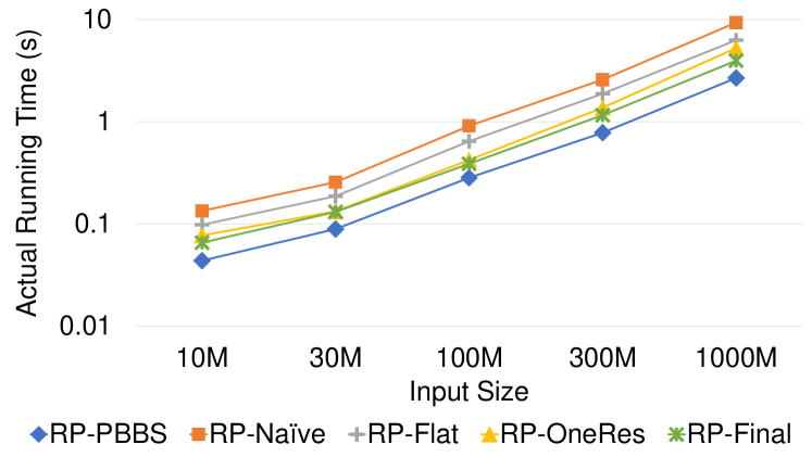
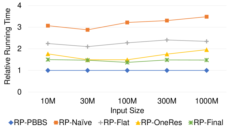
We test the performance of our implementations on inputs of size 10 million to 1 billion 64-bit integers, and compare them with the best non-in-place counterpart, which is from PBBS (RP-PBBS). The actual running times are shown in Figure 7 and Table 6. In Figure 7 (left), we see that all of the implementations have similar and consistent scalability with respect to input size. In Figure 7 (right), we show the running times relative to RP-PBBS. RP-Final only has a modest overhead of 30–40% over RP-PBBS, while only using 4% of the auxiliary space required by RP-PBBS. We can further reduce the additional space by shrinking the prefix size, at the expense of having more rounds, and hence more global synchronization. In Table 7, we present the running times under different amounts of additional space for RP-Final.
| Input size: | 10M | 30M | 100M | 300M | 1000M |
|---|---|---|---|---|---|
| RP-PBBS | 43.7 | 89.2 | 283 | 781 | 2680 |
| RP-Naïve | 134 | 256 | 910 | 2580 | 9330 |
| RP-Flat | 98.1 | 187 | 644 | 1880 | 6280 |
| RP-OneRes | 77.1 | 133 | 422 | 1370 | 5250 |
| RP-Final | 65.6 | 131 | 388 | 1160 | 3960 |
| Additional space | 0.4% | 1% | 2% | 4% |
|---|---|---|---|---|
| Running time (ms) | 537 | 425 | 411 | 388 |
7.5. List Contraction and Tree Contraction
Similar to random permutation, for list contraction and tree contraction, we design our PIP implementations based on the non-in-place implementations from PBBS (shun2012brief, ; shun2015sequential, ). In this case, the auxiliary space in list contraction and tree contraction is the array (shown in Algorithm 2), which has linear size. In list contraction (Algorithm 2) and tree contraction, represents whether node can be contracted in the current round. The deterministic reservations framework also needs to keep this information stored in another form, since it needs to pack the remaining iterates for the next round. We optimized the implementations to remove the array and store the information directly in the deterministic reservations framework—instead of indicating if the ’th iteration can be contracted (using the array), we use an array in the framework that stores this information only for the iterations in the current prefix. Hence, our implementation does not need to explicitly store the array, and thus only needs storage proportional to the prefix size.
| Input Size | List contraction | Tree contraction | ||||
| (million) | PBBS | PIP | PBBS | PIP | ||
| 10 | 59 | 49 | 73 | 46 | ||
| 20 | 79 | 70 | 141 | 82 | ||
| 50 | 142 | 131 | 323 | 198 | ||
| 100 | 247 | 205 | 600 | 350 | ||
| 200 | 494 | 418 | 1170 | 680 | ||
| Core | List contraction | Tree contraction | ||||
| count | PBBS | PIP | PBBS | PIP | ||
| 1 | 13900 | 3350 | 22800 | 12600 | ||
| 4 | 4370 | 1110 | 8020 | 4370 | ||
| 8 | 2180 | 636 | 3950 | 2210 | ||
| 18 | 1010 | 384 | 2060 | 1220 | ||
| 36 | 592 | 302 | 1390 | 1050 | ||
| 72 | 362 | 220 | 899 | 512 | ||
| 72HT | 247 | 205 | 603 | 350 | ||
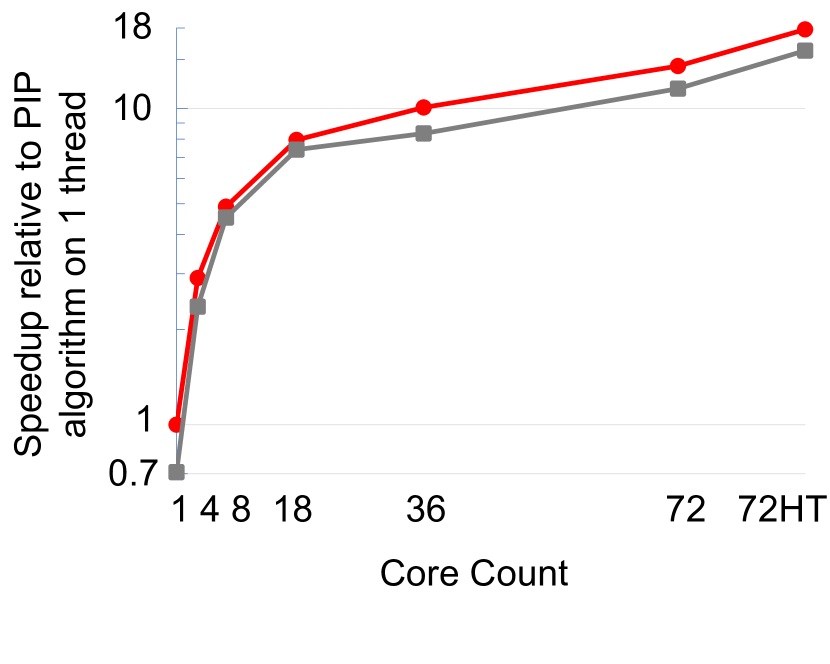
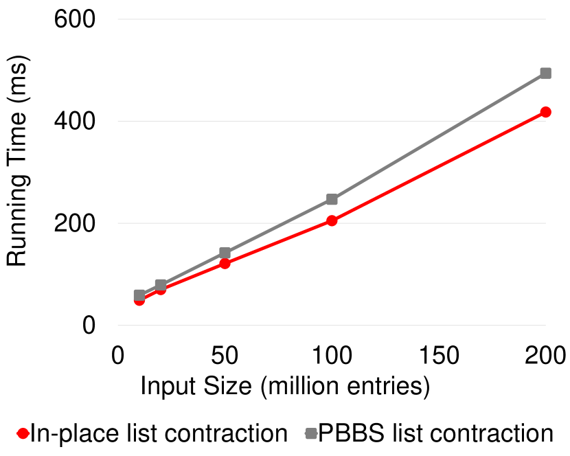
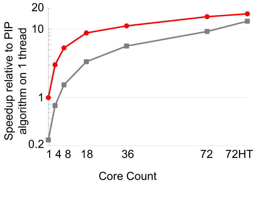
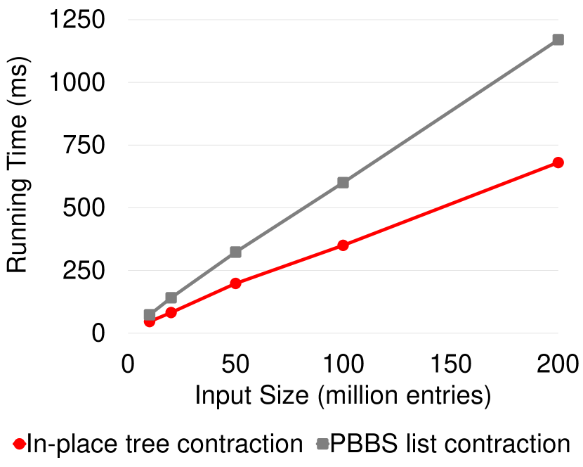
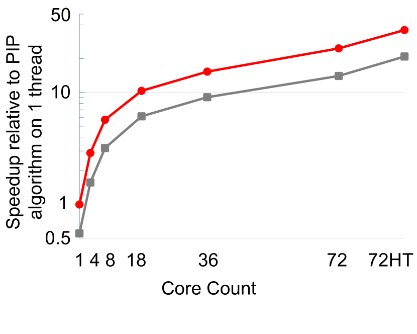
We test the performance of our implementations on inputs of between 10 million to 200 million entries, each of which contain two 64-bit pointers. The running times and speedups over the the PIP algorithm on 1 thread as a function of core counts are shown in Figure 6 and Tables 9–9. Since we eliminated the use of the array in our PIP algorithms and simplified the logic in the implementation (which required changes to the deterministic reservations framework), the parallel execution time improved by 15–20% for list contraction and 60–70% for tree contraction compared to non-in-place version in PBBS by Shun et al. (shun2015sequential, ). It is interesting to observe from Figure 6 and Table 9 that the speedups of the PIP algorithms over the PBBS implementations on one thread is larger than on 72 cores with hyper-threading. We conjecture that on one thread, the simpler logic improves prefetching, whereas when using all hyper-threads, prefetching does not help as much due to the memory bandwidth already being saturated.
7.6. Additional Space Usage
Table 10 shows the input size and total memory usage of our PIP algorithms. We see that for our two strong PIP algorithms (scan and filter), the auxiliary space overhead is negligible (less than 0.1%), and for the three relaxed PIP algorithms (random permutation, list contraction, and tree contraction), the best performance is achieved when the space overhead is between 0.9–3.7%, which is still much smaller than the input size. We can further reduce the space overhead for the relaxed PIP algorithms at the cost of higher running time (e.g., see Table 7). In contrast, the existing non-in-place algorithms for these problems require additional space proportional to the input size.
| Problem | Input size (MB) | Memory usage (MB) | Over-head |
|---|---|---|---|
| Scan | 7629.4 | 7636.2 | 0.1% |
| Filter | 7629.4 | 7636.9 | 0.1% |
| Random permutation | 762.9 | 791.2 | 3.7% |
| List contraction | 762.9 | 773.5 | 1.4% |
| Tree contraction | 1144.4 | 1154.9 | 0.9% |
8. Conclusion
In this paper, we defined two models for analyzing parallel in-place algorithms. We presented new parallel in-place algorithms for scan, filter, partition, merge, random permutation, list contraction, tree contraction, connectivity, biconnectivity, and minimum spanning forest. We implemented several of our algorithms, and showed experimentally that they are competitive or outperform state-of-the-art non-in-place parallel algorithms for the same problems.
Acknowledgements
We thank Guy Blelloch for letting us use his group’s machine for our experiments. This research was supported by DOE Early Career Award #DE-SC0018947, NSF CAREER Award #CCF-1845763, Google Faculty Research Award, DARPA SDH Award #HR0011-18-3-0007, and Applications Driving Architectures (ADA) Research Center, a JUMP Center co-sponsored by SRC and DARPA.
References
- [1] Umut A. Acar, Guy E. Blelloch, and Robert D. Blumofe. The data locality of work stealing. TCS, 35(3), 2002.
- [2] Nimar S. Arora, Robert D. Blumofe, and C. Greg Plaxton. Thread scheduling for multiprogrammed multiprocessors. Theory of Computing Systems (TOCS), 34(2), Apr 2001.
- [3] Michael Axtmann, Sascha Witt, Daniel Ferizovic, and Peter Sanders. In-place parallel super scalar samplesort (ips4o). In ESA, 2017.
- [4] Paul Beame, Allan Borodin, Prabhakar Raghavan, Walter L Ruzzo, and Martin Tompa. A time-space tradeoff for undirected graph traversal by walking automata. SIAM Journal on Computing, 28(3), 1998.
- [5] Naama Ben-David, Guy E. Blelloch, Jeremy T. Fineman, Phillip B. Gibbons, Yan Gu, Charles McGuffey, and Julian Shun. Parallel algorithms for asymmetric read-write costs. In SPAA, 2016.
- [6] Naama Ben-David, Guy E. Blelloch, Jeremy T. Fineman, Phillip B. Gibbons, Yan Gu, Charles McGuffey, and Julian Shun. Implicit decomposition for write-efficient connectivity algorithms. In IPDPS, 2018.
- [7] Kyle Berney, Henri Casanova, Alyssa Higuchi, Ben Karsin, and Nodari Sitchinava. Beyond binary search: parallel in-place construction of implicit search tree layouts. In IPDPS, 2018.
- [8] Guy E. Blelloch. Scans as primitive parallel operations. IEEE Trans. Computers, 38(11), 1989.
- [9] Guy E. Blelloch. Prefix sums and their applications. In Synthesis of Parallel Algorithms. Morgan Kaufmann, 1993.
- [10] Guy E Blelloch, Daniel Anderson, and Laxman Dhulipala. ParlayLib—a toolkit for parallel algorithms on shared-memory multicore machines. In SPAA, 2020.
- [11] Guy E. Blelloch, Laxman Dhulipala, and Yihan Sun. Introduction to parallel algorithms 15-853: Algorithms in the real world. 2018.
- [12] Guy E. Blelloch, Daniel Ferizovic, and Yihan Sun. Just join for parallel ordered sets. In SPAA, 2016.
- [13] Guy E Blelloch, Jeremy T Fineman, Phillip B Gibbons, Yan Gu, and Julian Shun. Sorting with asymmetric read and write costs. In SPAA, 2015.
- [14] Guy E. Blelloch, Jeremy T. Fineman, Phillip B. Gibbons, Yan Gu, and Julian Shun. Efficient algorithms with asymmetric read and write costs. In ESA, 2016.
- [15] Guy E. Blelloch, Jeremy T. Fineman, Phillip B. Gibbons, and Julian Shun. Internally deterministic algorithms can be fast. In PPoPP, 2012.
- [16] Guy E. Blelloch, Jeremy T. Fineman, Phillip B. Gibbons, and Harsha Vardhan Simhadri. Scheduling irregular parallel computations on hierarchical caches. In SPAA, 2011.
- [17] Guy E. Blelloch, Jeremy T. Fineman, Yan Gu, and Yihan Sun. Optimal parallel algorithms in the binary-forking model. In SPAA, 2020.
- [18] Guy E. Blelloch, Phillip B. Gibbons, and Harsha Vardhan Simhadri. Low depth cache-oblivious algorithms. In SPAA, 2010.
- [19] Guy E. Blelloch, Yan Gu, Julian Shun, and Yihan Sun. Parallelism in randomized incremental algorithms. In SPAA, 2016.
- [20] Guy E. Blelloch, Charles E. Leiserson, Bruce M. Maggs, C. Greg Plaxton, Stephen J. Smith, and Marco Zagha. A comparison of sorting algorithms for the Connection Machine CM-2. In SPAA, 1991.
- [21] Robert D. Blumofe and Charles E. Leiserson. Space-efficient scheduling of multithreaded computations. SIAM J. on Computing, 27(1), 1998.
- [22] Richard P. Brent and Hsiang T. Kung. A regular layout for parallel adders. IEEE transactions on Computers, (3), 1982.
- [23] Andrei Z Broder, Anna R Karlin, Prabhakar Raghavan, and Eli Upfal. Trading space for time in undirected - connectivity. SIAM Journal on Computing, 23(2), 1994.
- [24] Sankardeep Chakraborty, Anish Mukherjee, Venkatesh Raman, and Srinivasa Rao Satti. A Framework for In-place Graph Algorithms. In ESA, volume 112, 2018.
- [25] Sankardeep Chakraborty, Anish Mukherjee, and Srinivasa Rao Satti. Space efficient algorithms for breadth-depth search. In Fundamentals of Computation Theory, 2019.
- [26] Sankardeep Chakraborty, Kunihiko Sadakane, and Srinivasa Rao Satti. Optimal in-place algorithms for basic graph problems. In IWOCA, 2020.
- [27] Richard Cole and Vijaya Ramachandran. Resource oblivious sorting on multicores. ACM Trans. Parallel Comput., 3(4), Mar. 2017.
- [28] Thomas H. Cormen, Charles E. Leiserson, Ronald L. Rivest, and Clifford Stein. Introduction to Algorithms (3rd edition). MIT Press, 2009.
- [29] Richard Durstenfeld. Algorithm 235: Random permutation. Commun. ACM, 7(7), 1964.
- [30] Jeff A Edmonds. Time–space tradeoffs for undirected st-connectivity on a graph automata. SIAM Journal on Computing, 27(5), 1998.
- [31] Uriel Feige. A spectrum of time–space trade-offs for undirected - connectivity. Journal of Computer and System Sciences, 54(2), 1997.
- [32] Xiaojun Guan and Michael A. Langston. Time-space optimal parallel merging and sorting. IEEE Transactions on Computers, 1991.
- [33] Xiaojun Guan and Michael A. Langston. Parallel methods for solving fundamental file rearrangement problems. Journal of Parallel and Distributed Computing, 14(4), 1992.
- [34] Bing-Chao Huang and Michael A. Langston. Practical in-place merging. Communications of the ACM, 31(3), 1988.
- [35] Bing-Chao Huang and Michael A. Langston. Stable duplicate-key extraction with optimal time and space bounds. Acta Informatica, 26(5), 1989.
- [36] J. JaJa. Introduction to Parallel Algorithms. Addison-Wesley Professional, 1992.
- [37] Richard M. Karp and Vijaya Ramachandran. Parallel algorithms for shared-memory machines. In Handbook of Theoretical Computer Science, Volume A: Algorithms and Complexity (A). MIT Press, 1990.
- [38] Donald E. Knuth. Notes on “open” addressing. 1963.
- [39] Donald E. Knuth. The Art of Computer Programming, Volume II: Seminumerical Algorithms. Addison-Wesley, 1969.
- [40] Adrian Kosowski. Faster walks in graphs: a time-space trade-off for undirected st connectivity. In SODA, 2013.
- [41] William Kuszmaul and Alek Westover. Brief announcement: Cache-efficient parallel-partition algorithms using exclusive-read-and-write memory. In SPAA, 2020.
- [42] Michael A. Langston. Time-space optimal parallel computation. In Parallel Algorithm Derivation and Program Transformation. Springer, 1993.
- [43] Gary L. Miller and John H. Reif. Parallel tree contraction and its application. In FOCS, 1985.
- [44] Omar Obeya, Endrias Kahssay, Edward Fan, and Julian Shun. Theoretically-efficient and practical parallel in-place radix sorting. In SPAA, 2019.
- [45] Andrea Pietracaprina, Geppino Pucci, Francesco Silvestri, and Fabio Vandin. Space-efficient parallel algorithms for combinatorial search problems. Journal of Parallel and Distributed Computing, 76, 2015.
- [46] Margaret Reid-Miller, Gary L. Miller, and Francesmary Modugno. List ranking and parallel tree contraction. In Synthesis of Parallel Algorithms. Morgan Kaufmann, 1993.
- [47] John H. Reif. Synthesis of Parallel Algorithms. Morgan Kaufmann, 1993.
- [48] Raimund Seidel. Backwards analysis of randomized geometric algorithms. In New Trends in Discrete and Computational Geometry. 1993.
- [49] Julian Shun and Guy E. Blelloch. Phase-concurrent hash tables for determinism. In SPAA, 2014.
- [50] Julian Shun, Guy E. Blelloch, Jeremy T. Fineman, and Phillip B. Gibbons. Reducing contention through priority updates. In SPAA, 2013.
- [51] Julian Shun, Guy E. Blelloch, Jeremy T. Fineman, Phillip B. Gibbons, Aapo Kyrola, Harsha Vardhan Simhadri, and Kanat Tangwongsan. Brief announcement: the problem based benchmark suite. In SPAA, 2012.
- [52] Julian Shun, Yan Gu, Guy E. Blelloch, Jeremy T. Fineman, and Phillip B. Gibbons. Sequential random permutation, list contraction and tree contraction are highly parallel. In SODA, 2015.
- [53] Yihan Sun, Daniel Ferizovic, and Guy E. Blelloch. PAM: Parallel augmented maps. In PPoPP, 2018.
- [54] S. Q. Zheng, Balaji Calidas, and Yanjun Zhang. An efficient general in-place parallel sorting scheme. The Journal of Supercomputing, 14(1), 1999.
Appendix A Appendix
A.1. Deterministic Reservations
We now describe the framework of deterministic reservations in more detail. Each round of deterministic reservations consists of a reserve phase, followed by a synchronization point, and then a commit phase. In Algorithms 1 and 2, the reserve phase is first parallel for-loop that writes to locations in a shared data structure , corresponding to the steps (iterates). This is used to resolve conflicts among different steps that may modify the same memory locations. The commit phase is the second parallel for-loop that checks to see if the reservations for the step were successful (all of its writes end up as the final value in ); if so, the step is executed. Iterates that fail to execute will be packed by the framework and will retry in the next round. This is repeated until no iterates remain.
To achieve the best practical performance, instead of trying all iterates simultaneously (many of which will fail, and waste work), the framework only works on a prefix of all the iterates. After each round, the failed iterates are packed and new iterates are added to the prefix so that we have a sufficient number of iterates for the next round. In practice, we pick a prefix of 1–2% of the overall number of iterates, which gives a good trade-off between work and parallelism, and at the same time it naturally meets our requirement for controlling the execution size in the relaxed PIP algorithm.
For PIP algorithms, we usually need an additional phase in each round, which we refer to as the cleaning phase. In classic parallel algorithms based on deterministic reservations, we only initialize the reservation array at the beginning of the algorithm (line 1 in Algorithm 1 and 2). However, for PIP algorithms, we need to clean the data and reuse the space for the next round.
A.2. Random Permutation Implementations
RP-Naïve. Our first version uses parallel hash tables to replace the auxiliary arrays and , and we refer to this implementation as this algorithm RP-Naïve. Unfortunately, compared to RP-PBBS, RP-Naïve has poor performance in practice. On input sizes between 10 million to 1 billion, RP-Naïve requires 2.9–3.5x running time of the RP-PBBS algorithm, as shown in Figure 7. The reason is that, the original RP-PBBS implementation from PBBS needs roughly 4 sequential accesses and 2 random accesses per swap on each round, and the 2 random accesses per swap is to set and check per round. Since we cannot keep and explicitly but we need to use parallel hash tables, RP-Naïve incurs 6 random accesses per swap (setting and checking , , and ), and 3 more sequential accesses for cleaning. The cleaning for both and is done by simply clearing the entire hash tables, which we found to be more efficient than doing individual hash table deletions.
RP-Flat: packing as an array. In RP-PBBS, the value of is computed by a hash function. Since generating a good hash function in practice is expensive and this value is used in a variety of places, we store it in an array to avoid recomputation. We note that in Algorithm 1, the access of is always associated with index , and we only need to access the values of that are the sources of the swaps in the prefix for the current round. Hence, we only keep an array of the size of the prefix, and use it to store the corresponding value in for each iterate in the prefix. As such, we need to modify the code of deterministic reservations so that it also provides the index of each swap in the overall list of active iterates, so that we can look up its value in . By doing so, we reduce the number of hash table inserts/queries of each swap from three to two (by eliminating the random accesses to ). The cleaning phase incurs two serial accesses per swap since we need to clear the hash table for , which is twice the size of the prefix (as done in RP-Naïve, we clear the entire hash table). We refer to this implementation as RP-Flat.
RP-OneRes: using only one reservation. The previous implementations use two updates per swap (Lines 1 and 1 in Algorithm 1). However, we observe that we can apply just one update on Line 1, and avoid the update on Line 1. Then, the if-condition on Line 1 is modified to
Here indicates the initialized value of hash table, meaning that key is not found in the hash table. The advantage is that we reduce the number of hash table insertions of each swap from two to one, which enables us to use a hash table of half the size and reduce the overall memory footprint. The cleaning phase incurs one sequential access per swap to clear the hash table. We refer to this implementation as RP-OneRes.
RP-Final: packing the consecutive part of in an array. With the modified if-condition on Line 1, for the swap of iterate we need to check the value of . We can use a similar approach as done for in RP-Flat, so that when accessing , instead of a random access to a hash table, we only need a sequential access to an array. Unfortunately, we do not have the inverse mapping from each swap to its index in the active list. However, we do know that the indices are consecutive for all newly added swaps in a round. Hence, we modify the code for deterministic reservations so that it provides the range of the consecutive indices and the range of the keys. We can then use an array with the size of the active list. For reserving , we first check if the key falls in the range. If so, we map it to the associated index and update it in the array; otherwise, we insert it into the hash table. Checking the values in the commit phase is done similarly. In this way, the accesses of are mostly serial, and so we save one random access per swap on each round. For the cleaning phase, we clear the consecutive array, and for any swaps whose target is in the hash table, we delete it from the hash table (unlike our earlier implementations, we do not scan and clear the entire hash table). Most of the swaps will incur a sequential access for clearing it in the consecutive array. However, there is a random access to the hash table for clearing, if the swap target is in the hash table (i.e., it is not a newly added swap for this round). This happens infrequently since most of the swaps are successful if we pick a small prefix in each round. We refer to this implementation as RP-Final. The approximate numbers of sequential and random memory accesses per swap on each round are shown in Table 5.