Next-to-next-to-leading order event generation for $Z$-boson pair
production matched to parton shower

Abstract

We present a novel next-to-next-to-leading order (NNLO) QCD calculation matched to parton shower for the production of a pair of $Z$ bosons decaying to four massless leptons, $pp\to\ell^{+}\ell^{-}\ell^{\prime+}\ell^{\prime-}+X$, at the LHC. Spin correlations, interferences and off-shell effects are included throughout. Our result is based on the resummed beam-thrust spectrum, which we evaluate at next-to-next-to-leading-logarithmic (NNLL${}^{\prime}_{\mathcal{T}_{0}}$) accuracy for the first time for this process, and makes use of the Geneva Monte Carlo framework for the matching to Pythia8 shower and hadronisation models. We compare our predictions with data from the ATLAS and CMS experiments at $13\,\mathrm{TeV}$, finding a good agreement.

1 Introduction

Diboson production at the LHC is of paramount importance to the precision study of electroweak (EW) physics in the Standard Model (SM) and beyond, as it directly probes the non-Abelian EW couplings. The four-lepton channel that proceeds predominantly through intermediate $Z$-boson pairs is of particular importance due to its very clean signature. Consequently, several cross-section measurements and studies of anomalous couplings were carried out by both the ATLAS and CMS collaborations at 7 TeV [1, 2, 3, 4], 8 TeV [5, 6, 7, 8, 9] and 13 TeV [10, 11, 12, 13, 14, 15, 16]. Moreover, analyses of the four-lepton channel have helped to constrain the width and couplings of the Higgs boson [17, 18, 19, 20, 21, 22, 23, 24, 25, 26, 27, 28]. In addition, given that $Z^{\prime}$ resonances are common features in models of new physics, measurements of $Z$ pair production can help to set limits on Beyond the SM scenarios.

Theoretical predictions to $ZZ$ production have been known at NLO in QCD for some time [29, 30, 31, 32, 33, 34]. These were followed by calculations of NLO EW corrections, both for on-shell bosons [35, 36, 37] and for fully leptonic final states [38, 39], and more recently combinations of NLO QCD and EW contributions have appeared [40, 41]. The current state-of-the-art at fixed order in perturbation theory is NNLO [42, 43, 44, 45] in QCD for the process $q\bar{q}\to ZZ\to 4\ell$, combined with NLO EW effects [46]. NLO corrections (at $\mathcal{O}(\alpha_{s}^{3})$) to the loop-induced process $gg\to ZZ\to 4\ell$ are also available [47, 48, 49, 50].

In order to take advantage of the increasing precision of experimental data, it is useful to provide predictions in the form of fully exclusive Monte Carlo (MC) event generators. These allow hadron-level events to be produced that can be directly interfaced to detector simulations and experimental analyses.

For the $q\bar{q}\to ZZ\to 4\ell$ channel, the state-of-the-art in this regard is still matching NLO QCD correction to parton shower (NLOPS), as implemented in Powheg [51, 52], also including NLO EW effects [53]. For the $gg\to ZZ\to 4\ell$ channel NLOPS predictions were presented in Refs. [54, 55].

There has, however, been significant progress in the matching of NNLO calculations to parton showers (NNLOPS) in recent years, with four major approaches to the problem [56, 57, 58, 59, 60, 61, 62, 63]. In this Letter, we consider the Geneva framework developed in [57, 59, 64], which has been successfully applied to the Drell–Yan [59] and Higgsstrahlung [65] processes, as well as diphoton production [66] and hadronic Higgs decays [67].

Currently, the only available NNLOPS calculation featuring two massive bosons in the final state is for the process $pp\to W^{+}W^{-}\to\ell\nu\ell^{\prime}\nu^{\prime}$ [68] via the MiNLO^′ method [56], which made use of a differential reweighting to the Matrix predictions of Ref. [69] to achieve NNLO accuracy. Naïvely, the complexity of the final state would require a nine-dimensional reweighting, something unfeasible in practical terms. In Ref. [68], the authors were able to circumvent this limitation by rewriting the differential cross section in terms of angular coefficients, which they used to reweight each angular contribution separately. The dimensionality of the reweighting procedure was thus reduced to just three. This relied, however, on the approximation that the vector bosons are close to being on-shell, and so cannot be easily applied to the case of $pp\to Z/\gamma^{*}Z/\gamma^{*}\to 4\ell$, given the non-negligible contribution from photon exchange.

Since the Geneva method does not need a multi-differential reweighting to reach NNLO accuracy, we are able to include the full off-shell effects and deliver the first NNLOPS calculation for $ZZ$ production.

The process $pp\to\ell^{+}\ell^{-}\ell^{\prime+}\ell^{\prime-}+X$ features contributions from channels with very different resonance structures. In order to increase efficiency in event generation in such a situation, it is necessary to make use of a phase space generator which samples these channels separately. To this end, we have built an interface between Geneva and the multi-channel integrator Munich [70] which is completely general and allows for the integration of any SM process.

This Letter is organised as follows: we discuss the process definition and the relevant calculation in sec. 2, present our results and the comparison to LHC data in sec. 3 and draw our conclusions in sec. 4. Additional details concerning the calculation are provided in A and B.

2 Process definition

In this Letter, we consider the process $pp\to\ell^{+}\ell^{-}\ell^{\prime+}\ell^{\prime-}+X$, including off-shell effects, $Z/\gamma^{*}$ interference and spin correlations. The derivation of the Geneva formulae has been presented in several papers, see e.g. [59, 65]. Here we content ourselves with presenting the final results for the differential weights of the $0$-,$1$- and $2$- jet partonic cross sections.

These are defined in such a way that they correspond to physical and IR-finite events at a given perturbative accuracy, with the condition that IR singularities cancel on an event-by-event basis. The Geneva method achieves this by mapping IR-divergent final states with $M$ partons into IR-finite final states with $N$ jets, with $M\geq N$. Events are classified according to the value of $N$-jet resolution variables $\mathcal{T}_{N}$ which partition the phase space into different regions according to the number of resolved emissions. In particular, the Geneva Monte Carlo cross section $\mathrm{d}\sigma^{\textsc{mc}}_{N}$ receives contributions from both $N$-parton events and $M$-parton events where the additional emission(s) are below the resolution cut $\mathcal{T}_{N}^{\mathrm{cut}}$ used to separate resolved and unresolved emissions. The unphysical dependence on the boundaries of this partitioning procedure is removed by requiring that the resolution parameters are resummed at high enough accuracy. For the production of a pair of $Z$ bosons at NNLO accuracy, we need to introduce the $0$-jettiness resolution variables $\mathcal{T}_{0}$ and $1$-jettiness $\mathcal{T}_{1}$ defined as

$$\mathcal{T}_{N}=\sum_{k}\min\Bigl{\{}\hat{q}_{a}\cdot p_{k},\hat{q}_{b}\cdot p_{k},\hat{q}_{1}\cdot p_{k},\ldots,\hat{q}_{N}\cdot p_{k}\Bigr{\}}\,,$$ (1)

with $N=0$ or $1$, $q_{a},q_{b}$ representing the beam directions and $q_{k}$ any final state massless direction that minimise $\mathcal{T}_{N}$. These separate the $0$- and $1$-jet exclusive cross sections from the $2$-jet inclusive one.

We find that

$$\frac{\mathrm{d}\sigma^{\textsc{mc}}_{0}}{\mathrm{d}\Phi_{0}}(\mathcal{T}_{0}^{\mathrm{cut}}) =\frac{\mathrm{d}\sigma^{\rm NNLL^{\prime}}}{\mathrm{d}\Phi_{0}}(\mathcal{T}_{0}^{\mathrm{cut}})-\biggl{[}\frac{\mathrm{d}\sigma^{\rm NNLL^{\prime}}}{\mathrm{d}\Phi_{0}}(\mathcal{T}_{0}^{\mathrm{cut}})\biggr{]}_{\rm NNLO_{0}}$$

$$\quad+(B_{0}+V_{0}+W_{0})(\Phi_{0})$$

$$\quad+\int\!\frac{\mathrm{d}\Phi_{1}}{\mathrm{d}\Phi_{0}}\,(B_{1}+V_{1})(\Phi_{1})\,\theta[\mathcal{T}_{0}(\Phi_{1})<\mathcal{T}_{0}^{\mathrm{cut}}]$$

$$\quad+\int\!\frac{\mathrm{d}\Phi_{2}}{\mathrm{d}\Phi_{0}}\,B_{2}(\Phi_{2})\,\theta[\mathcal{T}_{0}(\Phi_{2})<\mathcal{T}_{0}^{\mathrm{cut}}]\,,$$ (2)

$$\frac{\mathrm{d}\sigma^{\textsc{mc}}_{1}}{\mathrm{d}\Phi_{1}}(\mathcal{T}_{0}>\mathcal{T}_{0}^{\mathrm{cut}};\mathcal{T}_{1}^{\mathrm{cut}})$$

$$\quad=\Bigg{\{}\frac{\mathrm{d}\sigma^{\rm NNLL^{\prime}}}{\mathrm{d}\Phi_{0}\mathrm{d}\mathcal{T}_{0}}\mathcal{P}(\Phi_{1})+(B_{1}+V_{1}^{C})(\Phi_{1})$$

$$\quad\quad\quad\quad-\biggl{[}\frac{\mathrm{d}\sigma^{\rm NNLL^{\prime}}}{\mathrm{d}\Phi_{0}\mathrm{d}\mathcal{T}_{0}}\mathcal{P}(\Phi_{1})\,\biggr{]}_{\mathrm{NLO}_{1}}\Bigg{\}}$$

$$\quad\times U_{1}(\Phi_{1},\mathcal{T}_{1}^{\mathrm{cut}})\,\theta(\mathcal{T}_{0}>\mathcal{T}_{0}^{\mathrm{cut}})$$

$$\quad+\int\!\biggl{[}\frac{\mathrm{d}\Phi_{2}}{\mathrm{d}\Phi_{1}^{\mathcal{T}}}\,B_{2}(\Phi_{2})\,\theta[\mathcal{T}_{0}(\Phi_{2})>\mathcal{T}_{0}^{\mathrm{cut}}]\,\theta(\mathcal{T}_{1}<\mathcal{T}_{1}^{\mathrm{cut}})$$

$$\quad\quad\quad\quad-\frac{\mathrm{d}\Phi_{2}}{\mathrm{d}\Phi_{1}^{C}}\,C_{2}(\Phi_{2})\,\theta(\mathcal{T}_{0}>\mathcal{T}_{0}^{\mathrm{cut}})\biggr{]}$$

$$\quad-B_{1}(\Phi_{1})\,U_{1}^{(1)}(\Phi_{1},\mathcal{T}_{1}^{\mathrm{cut}})\,\theta(\mathcal{T}_{0}>\mathcal{T}_{0}^{\mathrm{cut}})\,,$$ (3)

$$\frac{\mathrm{d}\sigma^{\textsc{mc}}_{1}}{\mathrm{d}\Phi_{1}}(\mathcal{T}_{0} \leq\mathcal{T}_{0}^{\mathrm{cut}})$$ (4)

$$= \ \overline{\Theta}^{\mathrm{FKS}}_{\mathrm{map}}(\Phi_{1})\,(B_{1}+V_{1})\,(\Phi_{1})\,\theta(\mathcal{T}_{0}<\mathcal{T}^{\mathrm{cut}}_{0})\,,$$

$$\frac{\mathrm{d}\sigma^{\textsc{mc}}_{\geq 2}}{\mathrm{d}\Phi_{2}}(\mathcal{T}_{0}>\mathcal{T}_{0}^{\mathrm{cut}},\mathcal{T}_{1}>\mathcal{T}_{1}^{\mathrm{cut}})$$

$$\quad=\Bigg{\{}\frac{\mathrm{d}\sigma^{\rm NNLL^{\prime}}}{\mathrm{d}\Phi_{0}\mathrm{d}\mathcal{T}_{0}}\mathcal{P}(\Phi_{1})+(B_{1}+V_{1}^{C})(\Phi_{1})$$

$$\quad\quad\quad\quad-\biggl{[}\frac{\mathrm{d}\sigma^{\rm NNLL^{\prime}}}{\mathrm{d}\Phi_{0}\mathrm{d}\mathcal{T}_{0}}\mathcal{P}(\Phi_{1})\,\biggr{]}_{\mathrm{NLO}_{1}}\Bigg{\}}$$

$$\quad\times U_{1}^{\prime}(\Phi_{1},\mathcal{T}_{1})\theta(\mathcal{T}_{0}\!\!>\!\!\mathcal{T}_{0}^{\mathrm{cut}})\Big{|}_{\Phi_{1}=\Phi_{1}^{\mathcal{T}}\!\!(\Phi_{2})}\!\!\!\!\mathcal{P}(\Phi_{2})\,\theta(\mathcal{T}_{1}\!\!>\!\!\mathcal{T}_{1}^{\mathrm{cut}})$$

$$\quad+\bigl{\{}B_{2}(\Phi_{2})\,[1-\Theta^{\mathcal{T}}(\Phi_{2})\,\theta(\mathcal{T}_{1}<\mathcal{T}_{1}^{\mathrm{cut}})]$$

$$\quad\quad\quad-B_{1}(\Phi_{1}^{\mathcal{T}})\,U_{1}^{{(1)}\prime}(\Phi_{1}^{\mathcal{T}},\mathcal{T}_{1})\,\mathcal{P}(\Phi_{2})\,\theta(\mathcal{T}_{1}>\mathcal{T}_{1}^{\mathrm{cut}})\bigr{\}}$$

$$\quad\times\theta[\mathcal{T}_{0}(\Phi_{2})>\mathcal{T}_{0}^{\mathrm{cut}}]\,,$$ (5)

$$\frac{\mathrm{d}\sigma^{\textsc{mc}}_{\geq 2}}{\mathrm{d}\Phi_{2}}(\mathcal{T}_{0}>\mathcal{T}_{0}^{\mathrm{cut}},\mathcal{T}_{1}\leq\mathcal{T}_{1}^{\mathrm{cut}})$$ (6)

$$\quad=B_{2}(\Phi_{2})\,\overline{\Theta}^{\mathcal{T}}(\Phi_{2})\,\theta(\mathcal{T}_{1}<\mathcal{T}_{1}^{\mathrm{cut}})\,\theta\left(\mathcal{T}_{0}(\Phi_{2})>\mathcal{T}_{0}^{\mathrm{cut}}\right)\,,$$

where the $B_{j}$, $V_{j}$ and $W_{j}$ are the $0$-, $1$- and $2$-loop matrix elements for $j$ QCD partons in the final state.

We have introduced the shorthand notation

$$\frac{\mathrm{d}\Phi_{M}}{\mathrm{d}\Phi_{N}^{\cal O}}=\mathrm{d}\Phi_{M}\,\delta[\Phi_{N}-\Phi^{\cal O}_{N}(\Phi_{M})]\,\Theta^{\cal O}(\Phi_{N})$$ (7)

to indicate that the integration over a region of the $M$-body phase space is performed while keeping the $N$-body phase space and the value of some specific observable $\cal O$ fixed, with $N\leq M$. The $\Theta^{\cal O}(\Phi_{N})$ term in the previous equation limits the integration to the phase space points included in the singular contribution for the given observable $\cal O$. For example, when generating $1$-body events we use

$$\frac{\mathrm{d}\Phi_{2}}{\mathrm{d}\Phi_{1}^{\mathcal{T}}}\equiv\mathrm{d}\Phi_{2}\,\delta[\Phi_{1}-\Phi^{\mathcal{T}}_{1}(\Phi_{2})]\,\Theta^{\mathcal{T}}(\Phi_{2})\,,$$ (8)

where the map used by the $1\to 2$ splitting has been constructed to preserve $\mathcal{T}_{0}$, i.e.

$$\mathcal{T}_{0}(\Phi_{1}^{\mathcal{T}}(\Phi_{2}))=\mathcal{T}_{0}(\Phi_{2})\,,$$ (9)

and $\Theta^{\mathcal{T}}(\Phi_{2})$ defines the projectable region of $\Phi_{2}$ which can be reached starting from a point in $\Phi_{1}$ with a specific value of $\mathcal{T}_{0}$. The use of a $\mathcal{T}_{0}$-preserving mapping is necessary to ensure that the pointwise singular $\mathcal{T}_{0}$ dependence is alike among all terms in eqs. (2) and (2) and that the cancellation of said singular terms is guaranteed on an event-by-event basis.

The expressions in eqs. (4) and (6) encode the nonsingular contributions to the $1$- and $2$-jet rates which arise from non-projectable configurations below the corresponding cut. This is highlighted by the appearance of the complementary $\Theta$ functions, $\overline{\Theta}^{\cal O}$, which account for any configuration that is not projectable either because it would result in an invalid underlying-Born flavour structure or because it does not satisfy the $\mathcal{T}_{0}$-preserving mapping (see also [65]).

The term $V_{1}^{C}$ denotes the soft-virtual contribution of a standard NLO local subtraction (in our implementation, we follow the FKS subtraction as detailed in [71]). We have that

$$V_{1}^{C}(\Phi_{1})=V_{1}(\Phi_{1})+\int\frac{\mathrm{d}\Phi_{2}}{\mathrm{d}\Phi_{1}^{C}}C_{2}(\Phi_{2})\,,$$ (10)

with $C_{2}$ a singular approximation of $B_{2}$: in practice we use the subtraction counterterms which we integrate over the radiation variables $\mathrm{d}\Phi_{2}/\mathrm{d}\Phi_{1}^{C}$ using the singular limit $C$ of the phase space mapping. $U_{1}$ is an NLL Sudakov factor which resums large logarithms of $\mathcal{T}_{1}$ and $U_{1}^{\prime}$ its derivative with respect to $\mathcal{T}_{1}$.

The term $\mathcal{P}(\Phi_{N+1})$ represents a normalised splitting probability which serves to extend the differential dependence of the resummed terms from the $N$-jet to the $(N\!+\!1)$-jet phase space. For example, in eq. (2), the term $\mathcal{P}(\Phi_{1})$ makes the resummed spectrum in the first term (which is naturally differential in the $\Phi_{0}$ variables and $\mathcal{T}_{0}$) differential also in the additional two variables needed to cover the full $\Phi_{1}$ phase space. These splitting probabilities are normalised, i.e. they satisfy

$$\int\!\frac{\mathrm{d}\Phi_{N+1}}{\mathrm{d}\Phi_{N}\mathrm{d}\mathcal{T}_{N}}\,\mathcal{P}(\Phi_{N+1})=1\,.$$ (11)

The two extra variables are chosen to be an energy ratio $z$ and an azimuthal angle $\phi$. The functional forms of the $\mathcal{P}(\Phi_{N+1})$ are based on the Altarelli-Parisi splitting kernels, weighted by parton distribution functions (PDFs) where appropriate.

For the specific details of the implementation of the above formulae we refer the reader to Ref. [59].

The resummed contributions in the previous formulae are obtained from Soft-Collinear Effective Theory (SCET), where a factorisation formula for the production of a colour singlet can be written as

$$\frac{\textrm{d}\sigma^{\rm SCET}}{\textrm{d}\Phi_{0}\textrm{d}\mathcal{T}_{0}}= \sum_{ij}H_{ij}(\Phi_{0},\mu)\int\!\mathrm{d}r_{a}\,\mathrm{d}r_{b}\,B_{i}(r_{a},x_{a},\mu)$$

$$\qquad B_{j}(r_{b},x_{b},\mu)\,S(\mathcal{T}_{0}-\tfrac{r_{a}+r_{b}}{Q},\mu)\,.$$ (12)

The sum in the equation above runs over all possible $q\bar{q}$ pairs $ij=\{u\bar{u},\bar{u}u,d\bar{d},\bar{d}d,\ldots\}$. It also depends on the hard $H_{ij}$, soft $S$ and beam $B_{i,j}$ functions which describe the square of the hard interaction Wilson coefficients, the soft emissions between external partons and the hard emissions collinear to the beams respectively.

In SCET, the resummation of large logarithms is achieved by means of renormalisation group (RG) evolution between the typical energy scale of each component ($\mu_{H},\mu_{B}$ and $\mu_{S}$) and a common scale $\mu$. This proceeds via convolutions of the single scale factors with the evolution functions $U_{i}(\mu_{i},\mu)$. The resulting resummed formula for the $\mathcal{T}_{0}$ spectrum is then given by

$$\frac{\textrm{d}\sigma^{\text{NNLL}^{\prime}}}{\textrm{d}\Phi_{0}\textrm{d}\mathcal{T}_{0}}=\; \sum_{ij}H_{ij}(\Phi_{0},\mu_{H})\,U_{H}(\mu_{H},\mu)\,$$

$$\big{\{}\big{[}B_{i}(t_{a},x_{a},\mu_{B})\otimes U_{B}(\mu_{B},\mu)\big{]}\,$$

$$\times\big{[}B_{j}(t_{b},x_{b},\mu_{B})\otimes U_{B}(\mu_{B},\mu)\big{]}\big{\}}\,$$

$$\otimes\big{[}S(\mu_{s})\otimes U_{S}(\mu_{S},\mu)\big{]}\,,$$ (13)

where the convolutions between the different functions are written in a schematic form. In order to reach NNLL^′ accuracy, we need to know the boundary conditions of the evolution, namely the hard, beam and soft functions up to NNLO accuracy, and the cusp (non-cusp) anomalous dimensions up to three-(two-)loop order. The beam and soft functions at NNLO accuracy are available in the literature [72, 73, 74], as well as the cusp (non-cusp) anomalous dimensions up to three-(two-)loop order [75, 76, 77, 78, 79].

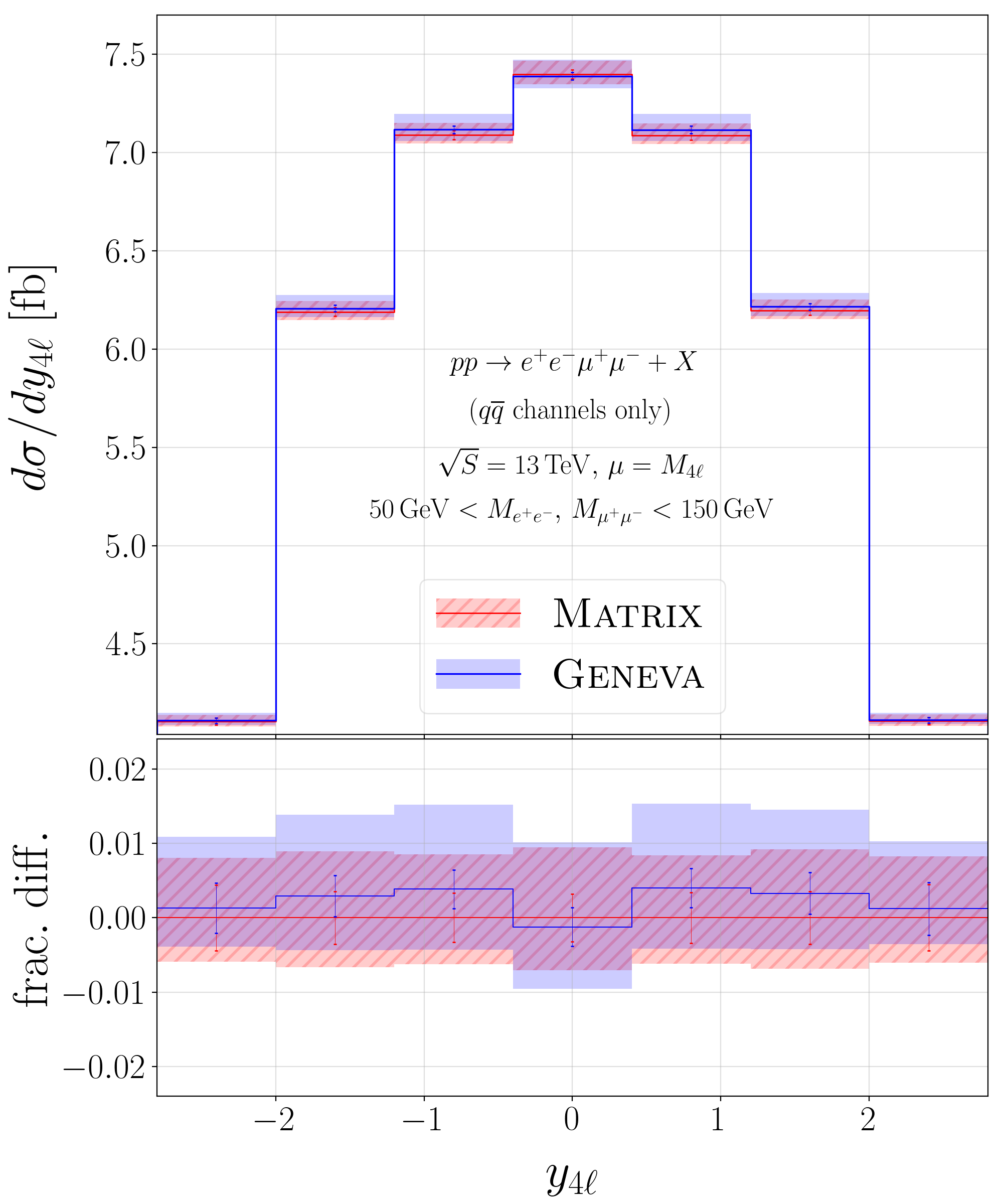
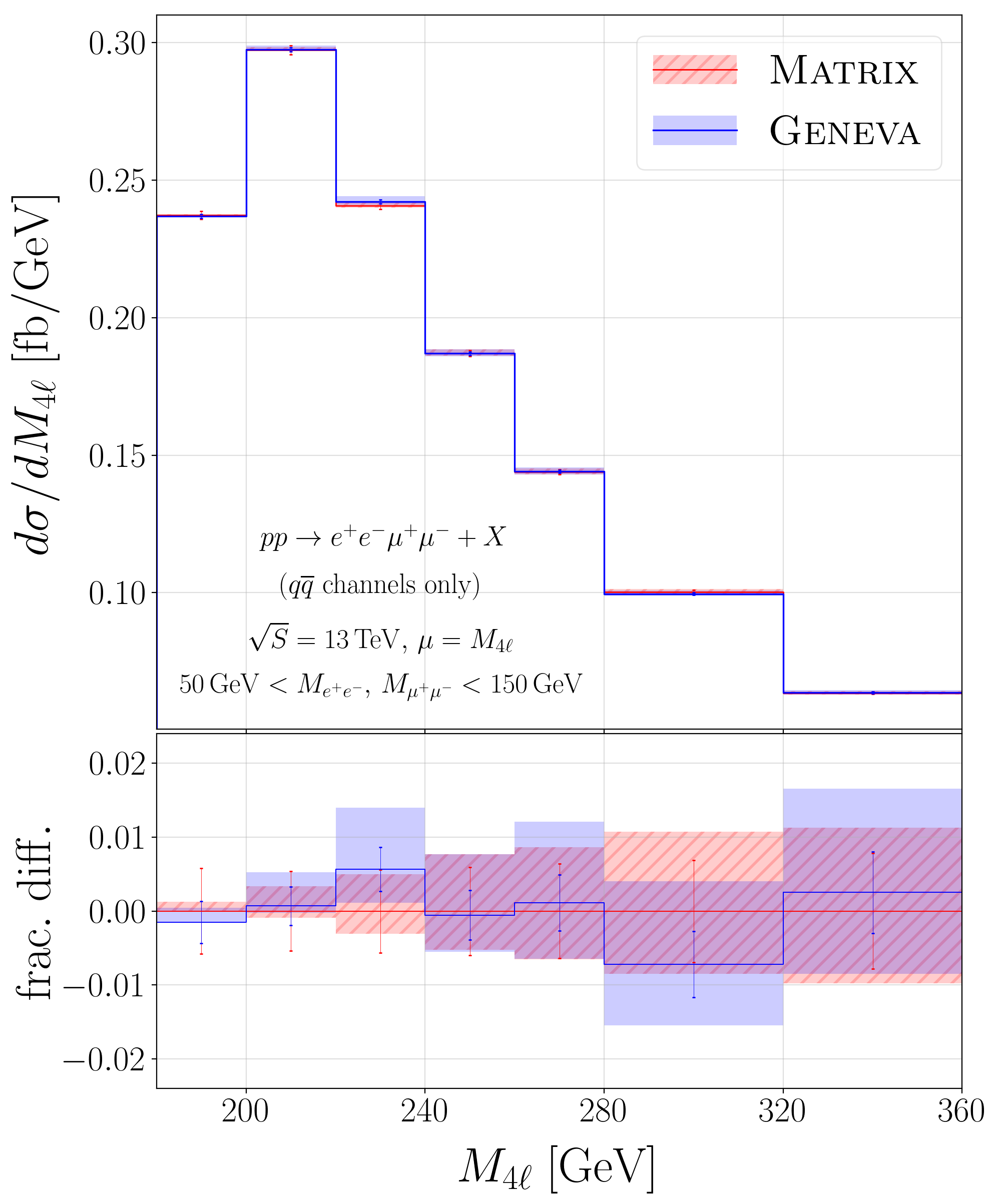
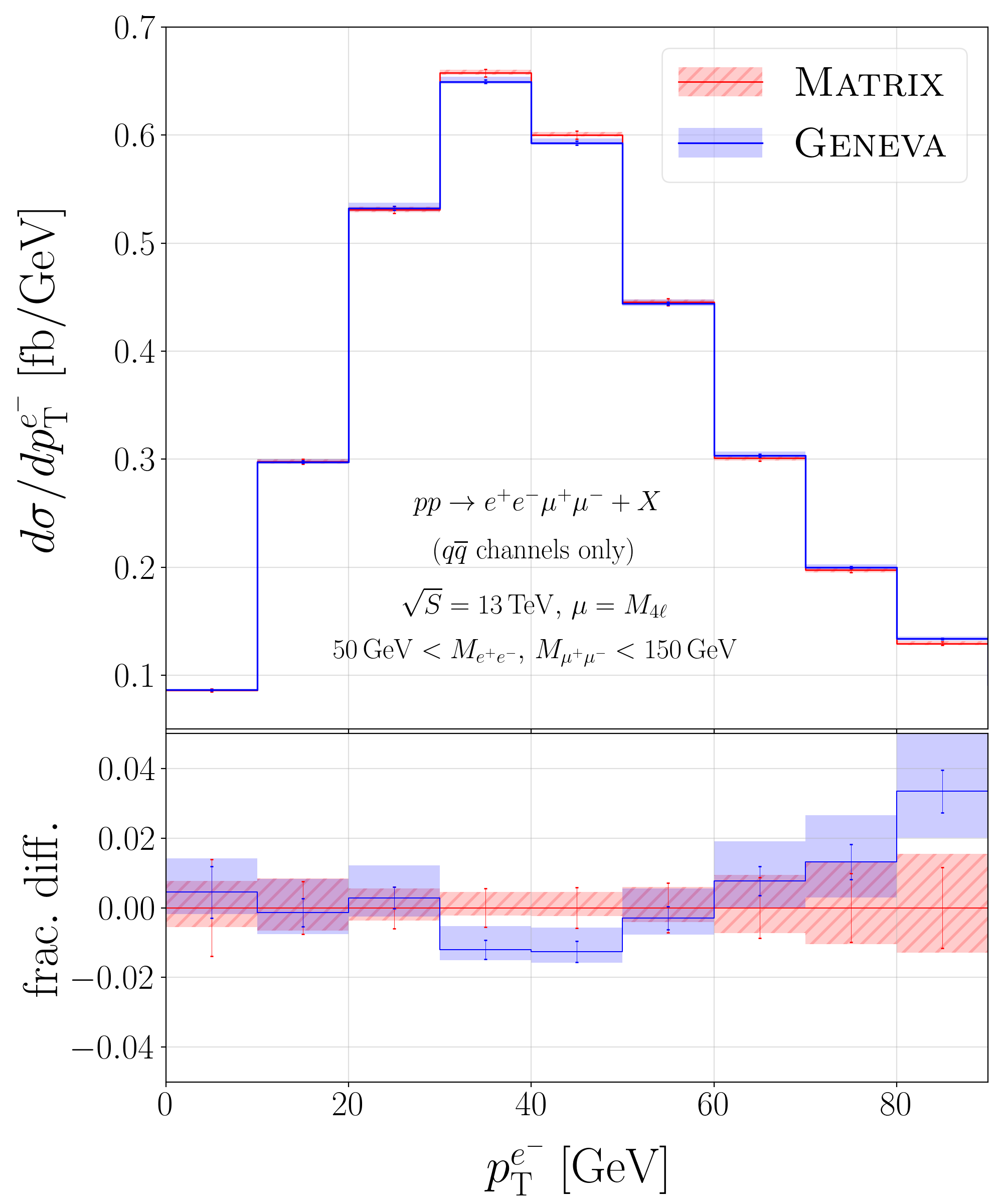
Figure 1: Comparison between the Matrix and Geneva predictions at NNLO accuracy. We show the rapidity of the four leptons (left), the mass of the four leptons (centre) and the transverse momentum of the electron (right). Scale uncertainty bands include 3-point renormalisation and factorisation scale variations. Statistical errors connected to the Monte Carlo integration are shown as vertical error bars.

The two-loop hard function $H_{ij}^{(2)}$ was instead computed starting from the form factors calculated in Refs. [80, 81] and using the numerical implementation in the public code VVamp [82]. Finally, we use OpenLoops2 [83, 84, 85] for the calculation of all the remaining matrix elements.

Starting from these accurate parton-level predictions we can interface to the Pythia8 parton shower to produce the high-multiplicity final states that can in turn be compared to experimental data. The shower adds extra radiation to the exclusive $0$- and $1$-jet cross sections and extends the inclusive $2$-jet cross section by including higher jet multiplicities. This means that we can expect the shower to modify the distributions of exclusive observables sensitive to the radiation, preserving the leading logarithmic accuracy for observables other than $\mathcal{T}_{0}$. At the same time, we have verified that the shower does not modify any distribution which is inclusive over the radiation, as was the case for the Geneva implementation of similar colour-singlet production processes. As a consequence we maintain NNLO accuracy for inclusive observables.

All the details about the interface between Geneva and Pythia8 can be found in section 3 of [59].

3 Results and comparison to LHC data

In the following, we focus on the process

$$pp\rightarrow e^{+}e^{-}\mu^{+}\mu^{-}+X$$ (14)

at a hadronic centre-of-mass energy of 13 $\,\mathrm{TeV}$ and require that the masses of both lepton–antilepton pairs are between 50 and 150 $\,\mathrm{GeV}$. We use the PDF set NNPDF31_nnlo_as_0118 [86] from LHAPDF6 [87] and set both the renormalisation and factorisation scales to the mass $M_{4\ell}$ of the four-lepton system. We choose the resolution cutoffs to be $\mathcal{T}_{0}^{\mathrm{cut}}=1$ GeV and $\mathcal{T}_{1}^{\mathrm{cut}}=1$ GeV.

For the validation, we focus only on the quark–antiquark channels and neglect the loop-induced gluon fusion channel, which only starts appearing in the calculation at NNLO and can therefore be added as a nonsingular fixed-order contribution. At this energy, the latter contribution amounts to $\sim 6$% of the total cross section and, as such, its inclusion will be important when comparing to data.

In Fig. 1 we validate the NNLO accuracy of the Geneva results by comparing with those obtained via an independent NNLO calculation implemented in Matrix. In particular, we show the distributions of the rapidity $y_{4\ell}$, mass $M_{4\ell}$ of the four leptons and the transverse momentum $p_{\mathrm{T}}^{e^{-}}$ of the electron. We observe a good agreement, with the only differences appearing in the shape of the $p_{\mathrm{T}}^{e^{-}}$ distribution. This is likely to be a consequence of the additional higher-order effects provided by Geneva, as observed in previous Geneva predictions for other colour-singlet production processes. We observe, however, that in almost all the bins the theoretical uncertainty bands computed by Geneva and Matrix still overlap.

Next we turn on the shower effects by interfacing to Pythia8. In order to maintain a simple analysis routine and focus only on QCD corrections, we do not include QED effects and multiple-particle interactions (MPI) in the shower.

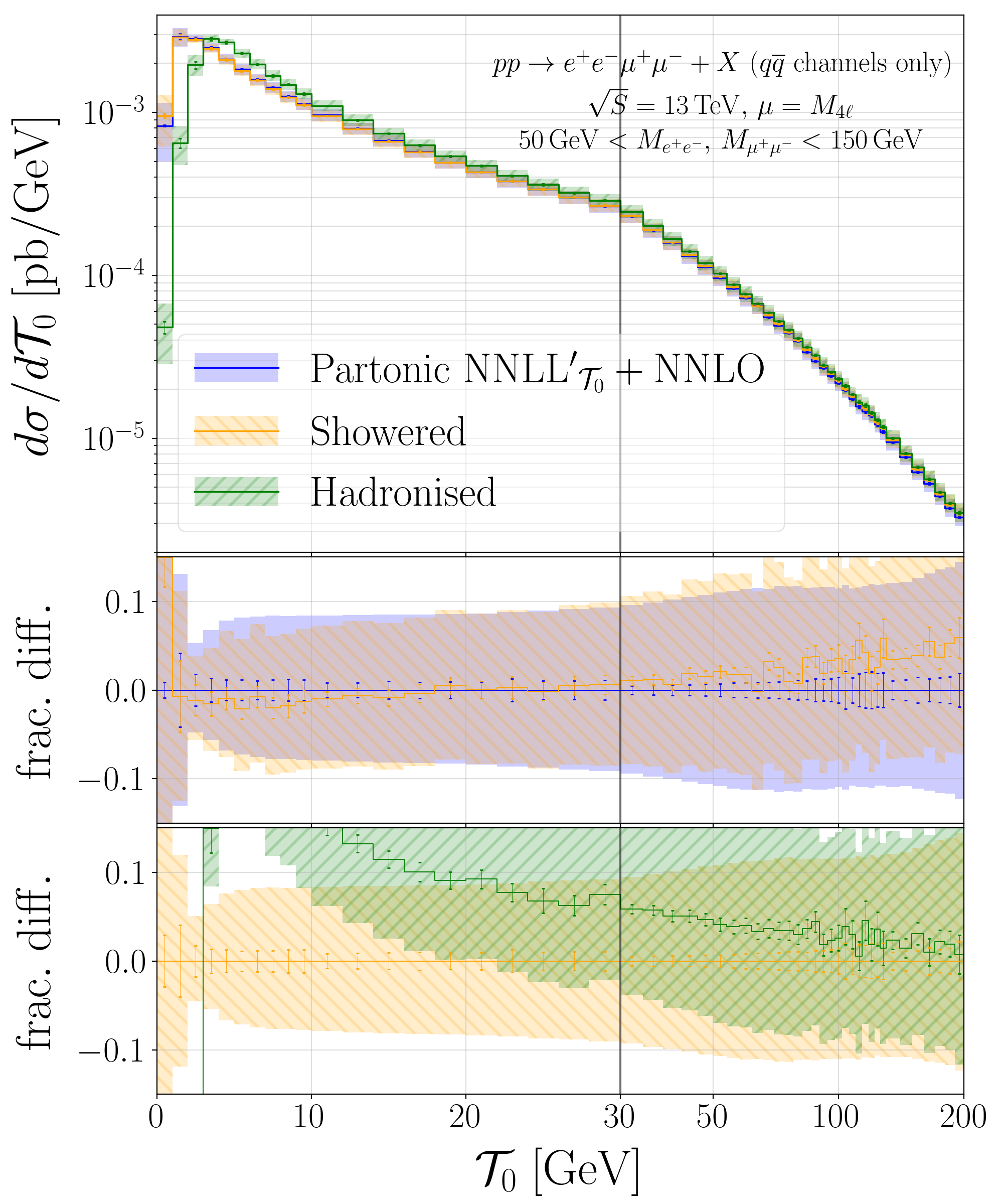
Figure 2: Comparison between the partonic, showered and hadronised results for the beam-thrust $\mathcal{T}_{0}$ distribution in Geneva and Geneva +Pythia8.

In Fig. 2 we present our predictions for the NNLL${}^{\prime}_{\mathcal{T}_{0}}$+NNLO beam-thrust spectrum (partonic result) and study the effect of shower and hadronisation on the $\mathcal{T}_{0}$ distribution. In order to highlight the peak and transition regions where the resummation effects are more important, we show the results on a semi-logarithmic scale, which is linear up to the value of $30$ GeV and logarithmic beyond. In the first ratio plot, we compare the $\mathcal{T}_{0}$ distribution before and after the shower, observing that the NNLL${}^{\prime}_{\mathcal{T}_{0}}$+NNLO accuracy reached at parton level is numerically very well preserved. The largest difference is, as expected, in the first bin where the shower generates all the events with $\mathcal{T}_{0}<\mathcal{T}_{0}^{\mathrm{cut}}$ which were previously integrated out in the inclusive $0$-jet cross section. In the second ratio plot we instead show the effect of hadronisation on the showered distribution. Owing to its nonperturbative origin, hadronisation affects mostly the region of small $\mathcal{T}_{0}$ and becomes less and less important in the tail of the distribution.

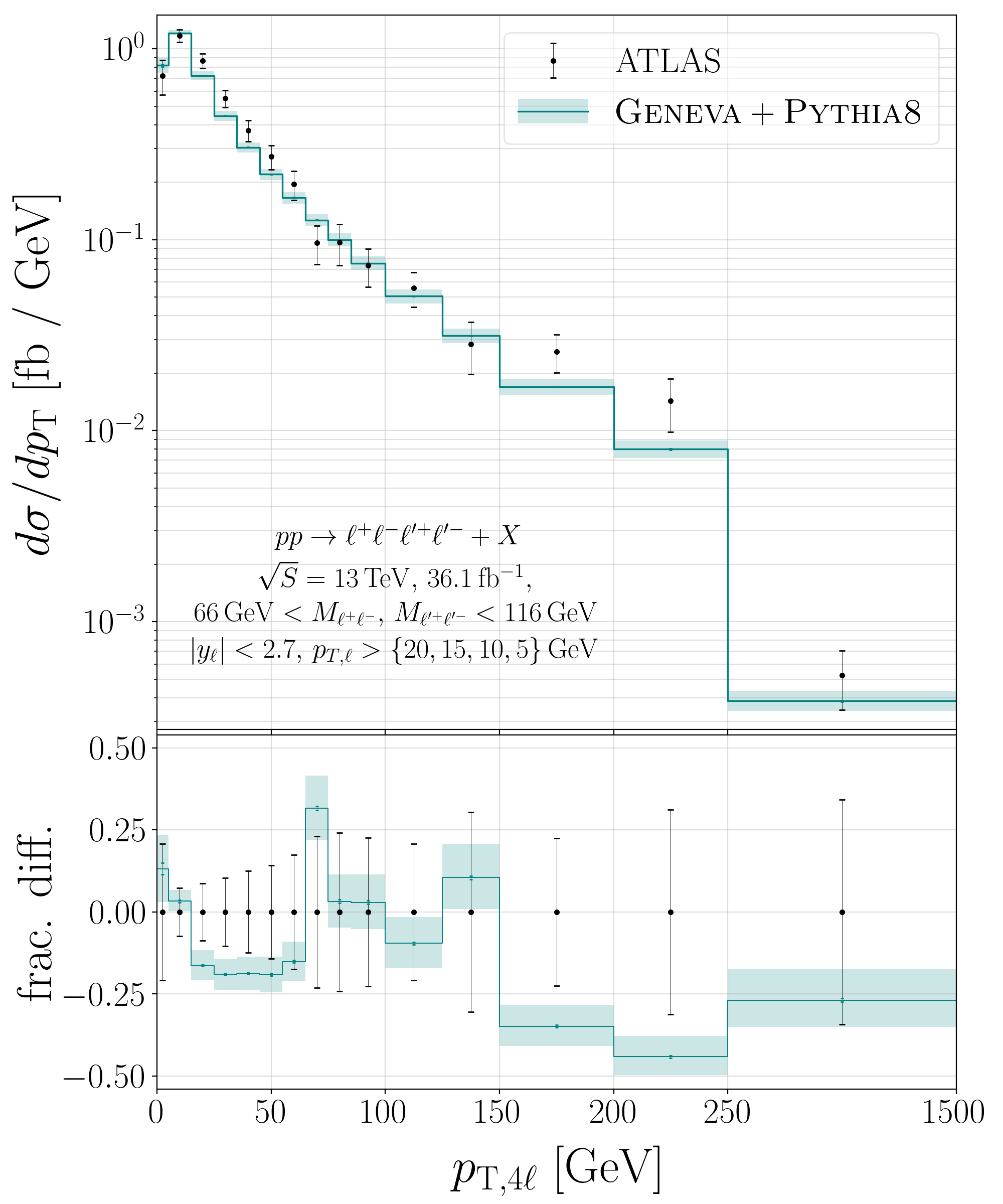
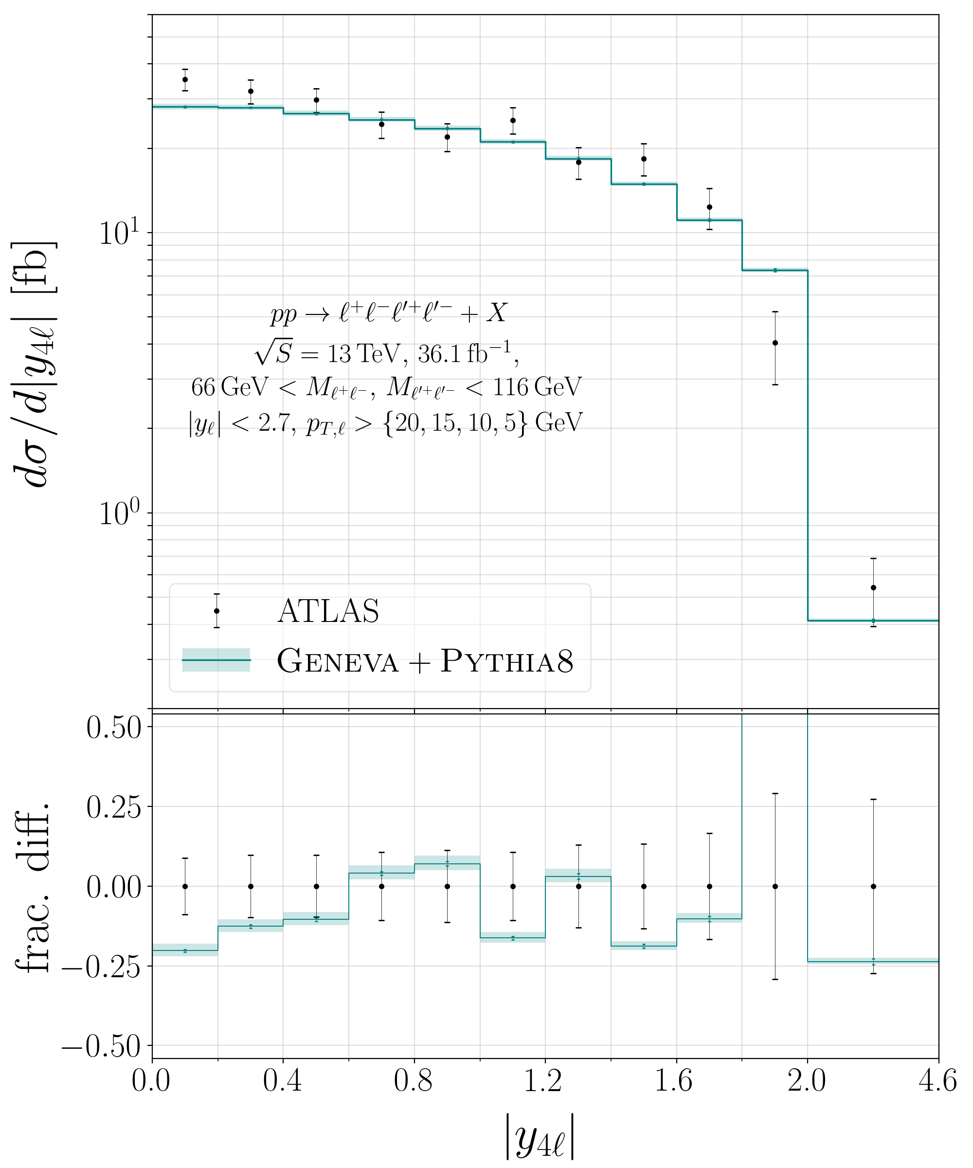
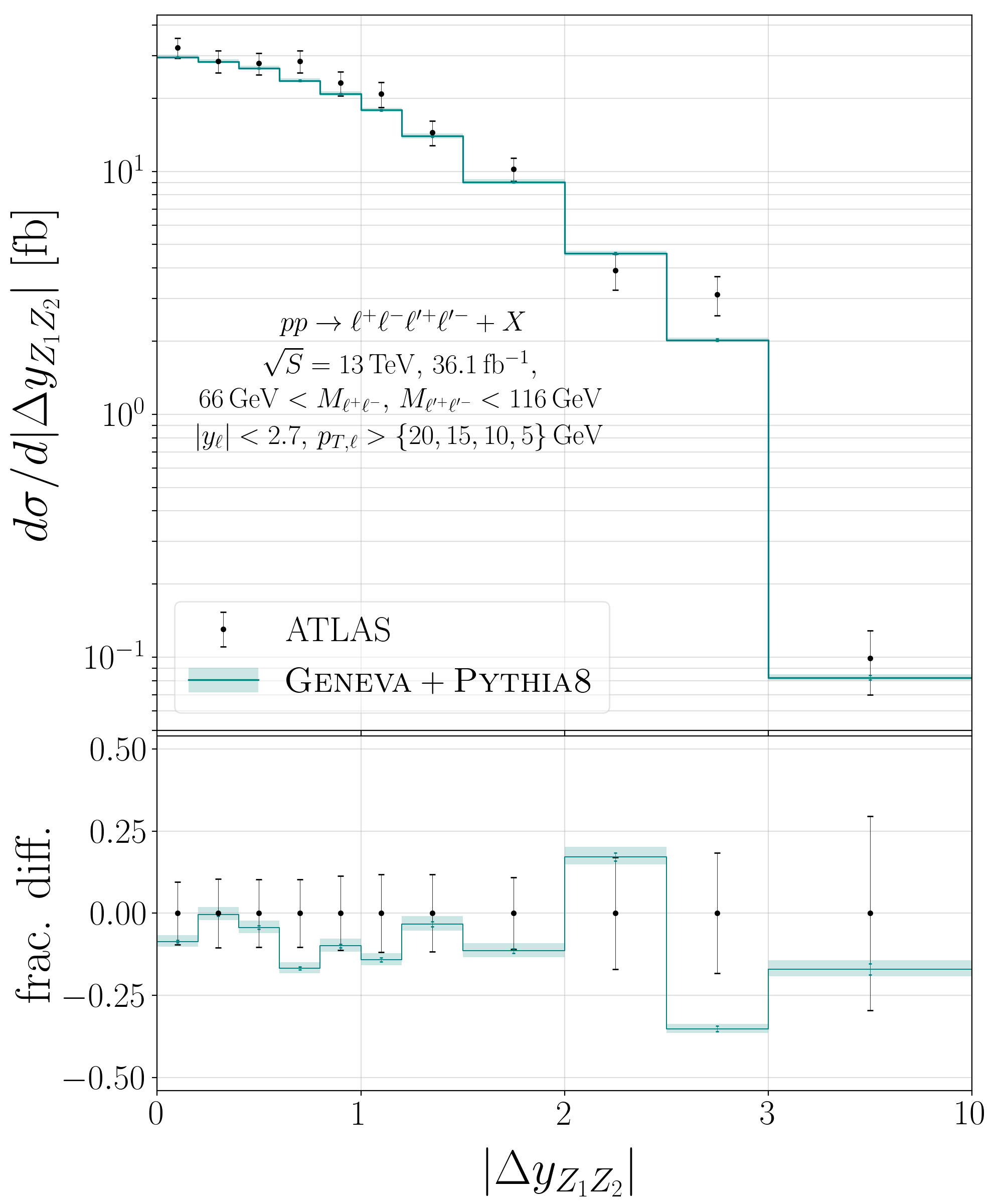
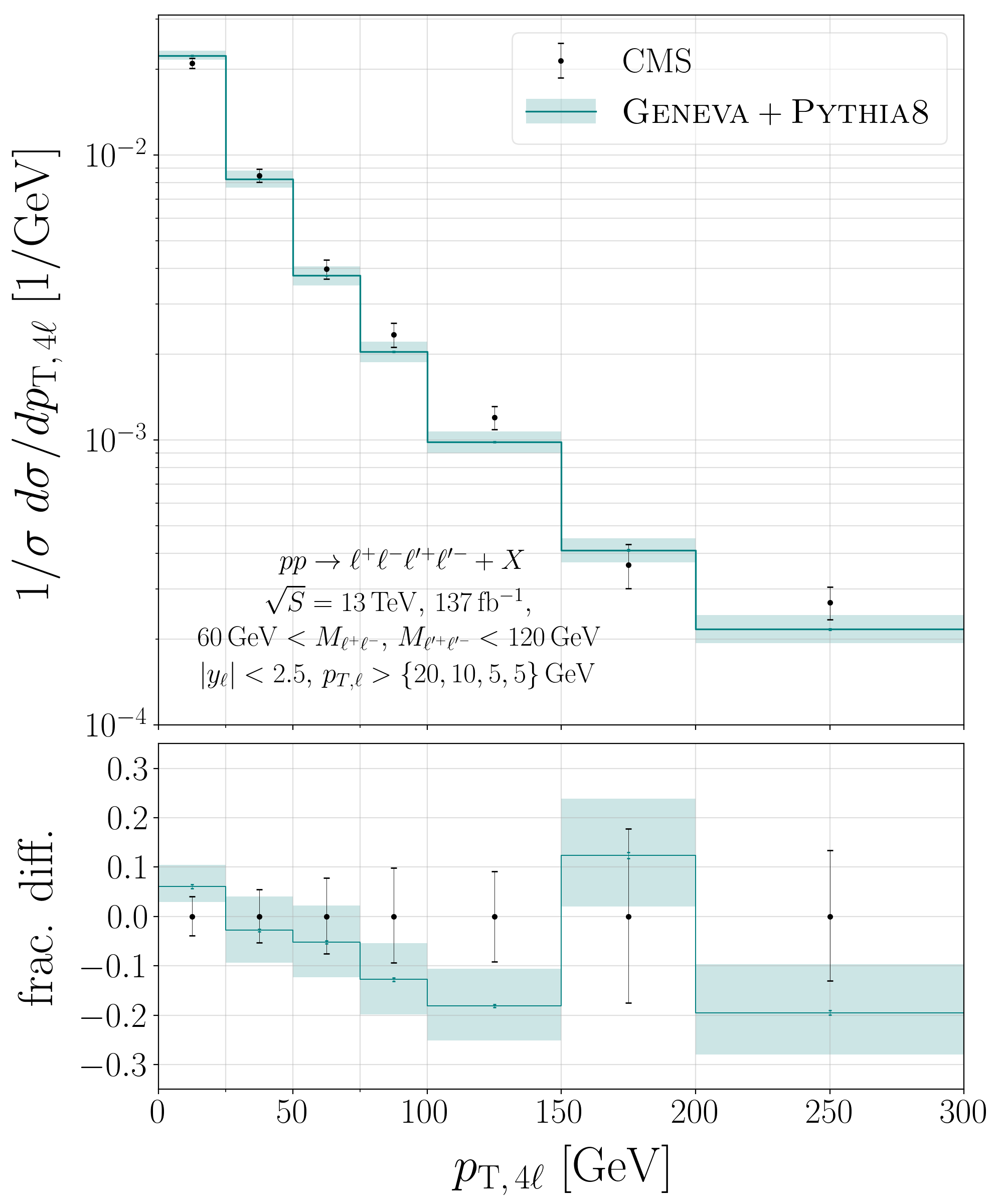
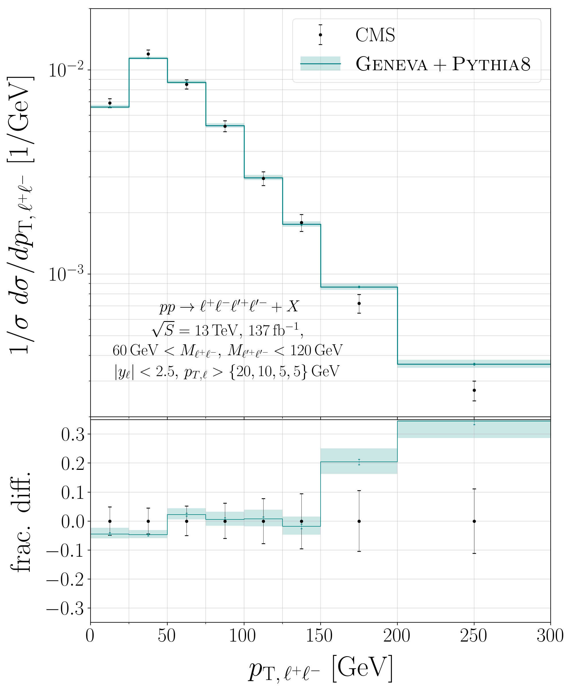
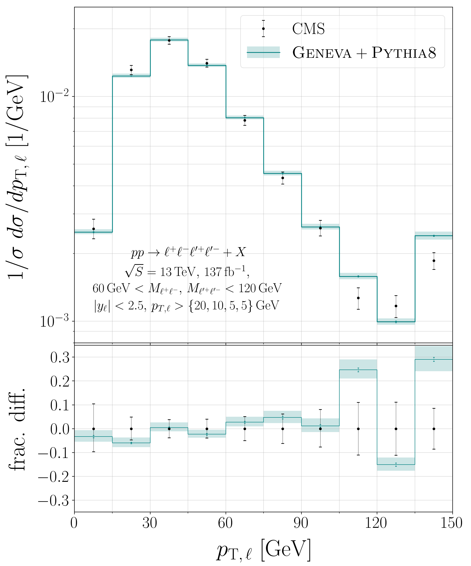
Figure 3: Comparison to ATLAS and CMS measurements from the LHC at 13 TeV. Selection cuts, bin widths and observable definitions are as detailed in the original ATLAS [11] and CMS [16] publications.

Finally, in Fig. 3 we compare our predictions with data obtained at the LHC at 13 $\,\mathrm{TeV}$ both from the ATLAS [11] and CMS [16] experiments. For this comparison we now include the loop-induced gluon fusion channel and MPI effects. The binning of observables and the acceptance cuts applied to the events in each analysis have been modelled according to the experimental requirements. They are briefly listed in the figure, but we refer the reader to the original papers for all the details.

In the first row we show the comparison with ATLAS data, obtained with an integrated luminosity of $36.1$ fb^-1. We consider the distributions for the transverse momentum of the four leptons $p_{\mathrm{T},4\ell}$, and two more inclusive distributions, the absolute value $|y_{4\ell}|$ of the rapidity of the four leptons and the absolute value $|\Delta y_{Z_{1}Z_{2}}|$ of the difference in rapidity between the two reconstructed $Z$ bosons. The agreement with data is reasonably good but the reduced experimental statistics make it difficult to draw more precise conclusions. We only notice a possible tension in the distribution of $|y_{4\ell}|$, where for small values of the rapidity the data seem to be systematically above the Geneva predictions. This behaviour has, however, been observed previously with several other Monte Carlo event generators in the original ATLAS publication [11].

In the second row, we show the comparison with CMS data, obtained with an integrated luminosity of $137$ fb^-1. We focus on the normalised distributions for $p_{\mathrm{T},4\ell}$, the transverse momentum $p_{\mathrm{T},\ell^{+}\ell^{-}}$ of the vector bosons and the transverse momentum $p_{\mathrm{T},\ell}$ of the leptons. The latter two distributions are obtained by averaging over all vector bosons and leptons present in an event. Due to the increased luminosity and the fact that we are comparing normalised distributions, here we observe smaller experimental uncertainties and a better agreement between the data and the Geneva predictions. We highlight the fact that according to the original definition of bins in Ref. [16], the last bin of each distribution we show must be interpreted as an overflow bin containing the contributions from the lower border up to the maximum possible value for that observable. This justifies for example the peculiar behaviour of the last bin of the $p_{\mathrm{T},\ell}$ distribution.

We conclude by noticing that the transverse momentum $p_{\mathrm{T},\ell^{+}\ell^{-}}$ of the vector bosons shows a sizable difference for values larger than $150$ GeV, where EW effects are known to be important [46] and should thus be included to improve the agreement with data.

4 Conclusions

In this Letter, we have presented the first event generator for the production of a pair of $Z$ bosons decaying into four leptons at NNLO accuracy matched to the Pythia 8 parton shower.

This was obtained using the resummation of the $0$-jettiness $\mathcal{T}_{0}$ resolution variable at NNLL^′ accuracy, matched to a fixed-order calculation at NNLO precision. The calculation was performed within the Geneva Monte Carlo framework, which allowed us to interface to the Pythia8 parton shower and hadronisation models.

After successfully validating the NNLO accuracy of the results against Matrix, we studied the effect of the shower on the differential distributions, observing that they are numerically small for inclusive quantities, as expected. Consequently, their NNLO accuracy is correctly maintained. We also verified that the hadronisation has a significant impact only for exclusive observables in the region of small $\mathcal{T}_{0}$, where the nonperturbative effects are not negligible.

Finally, we compared to LHC data, both from the ATLAS and CMS experiments. We found good agreement, except for a tension observed in the region of small absolute rapidity of the four lepton system. A similar behaviour had already been observed for other Monte Carlo generators. We also observed a general overestimation of the production rate for vector bosons at large transverse momentum, motivating the need for the inclusion of EW corrections to improve the agreement with data in this region.

Possible future directions for improvement for this calculation would be the inclusion of the NLO QCD corrections to the gluon fusion channel and of the aforementioned NLO EW corrections.

The code used for the simulations presented in this work is available upon request from the authors and will be made public in a future release of Geneva.

Appendix A Nonsingular power corrections

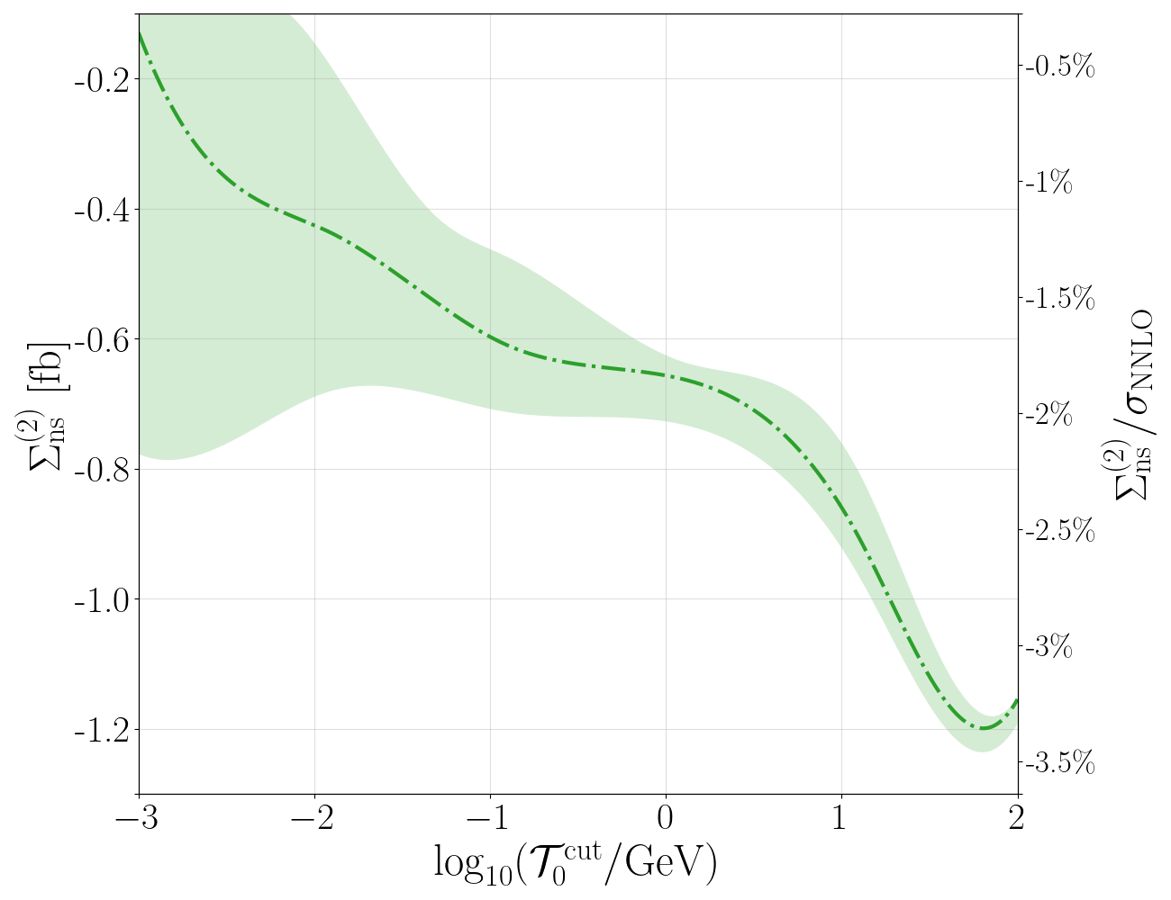
Figure 4: Size of the neglected power corrections $\Sigma^{(2)}_{\mathrm{ns}}$ as a function of the resolution parameter $\mathcal{T}_{0}^{\mathrm{cut}}$. The target result $\sigma_{\rm NNLO}$ is the fixed-order cross section, as computed by Matrix.

The Geneva calculation is based on $N$-jettiness subtraction, using a resolution cutoff $\mathcal{T}_{0}^{\mathrm{cut}}$. The contributions below the cut, given in eq. (2), require a local NNLO subtraction for their implementation. In Geneva, exploiting the $N$-jettiness subtraction, we substitute the expression given in eq. (2) with

$$\frac{\widetilde{\mathrm{d}\sigma^{\textsc{mc}}_{0}}}{\mathrm{d}\Phi_{0}}(\mathcal{T}_{0}^{\mathrm{cut}}) =\frac{\mathrm{d}\sigma^{\rm NNLL^{\prime}}}{\mathrm{d}\Phi_{0}}(\mathcal{T}_{0}^{\mathrm{cut}})-\biggl{[}\frac{\mathrm{d}\sigma^{\rm NNLL^{\prime}}}{\mathrm{d}\Phi_{0}}(\mathcal{T}_{0}^{\mathrm{cut}})\biggr{]}_{\rm NLO_{0}}$$

$$\quad+(B_{0}+V_{0})(\Phi_{0})$$

$$\quad+\int\!\frac{\mathrm{d}\Phi_{1}}{\mathrm{d}\Phi_{0}}\,B_{1}(\Phi_{1})\,\theta[\mathcal{T}_{0}(\Phi_{1})<\mathcal{T}_{0}^{\mathrm{cut}}]\,.$$ (15)

In other words, we neglect the contribution

$$\frac{d\Sigma^{(2)}_{\mathrm{ns}}}{\mathrm{d}\Phi_{0}}(\mathcal{T}_{0}^{\mathrm{cut}}) =\frac{\mathrm{d}\sigma^{\textsc{mc}}_{0}}{\mathrm{d}\Phi_{0}}(\mathcal{T}_{0}^{\mathrm{cut}})-\frac{\widetilde{\mathrm{d}\sigma^{\textsc{mc}}_{0}}}{\mathrm{d}\Phi_{0}}(\mathcal{T}_{0}^{\mathrm{cut}})$$

$$=\biggl{[}\frac{\mathrm{d}\sigma^{\rm NNLL^{\prime}}}{\mathrm{d}\Phi_{0}}(\mathcal{T}_{0}^{\mathrm{cut}})\biggr{]}_{\rm NLO_{0}}$$

$$\quad-\biggl{[}\frac{\mathrm{d}\sigma^{\rm NNLL^{\prime}}}{\mathrm{d}\Phi_{0}}(\mathcal{T}_{0}^{\mathrm{cut}})\biggr{]}_{\rm NNLO_{0}}$$

$$\quad+W_{0}(\Phi_{0})$$

$$\quad+\int\!\frac{\mathrm{d}\Phi_{1}}{\mathrm{d}\Phi_{0}}\,V_{1}(\Phi_{1})\,\theta[\mathcal{T}_{0}(\Phi_{1})<\mathcal{T}_{0}^{\mathrm{cut}}]$$

$$\quad+\int\!\frac{\mathrm{d}\Phi_{2}}{\mathrm{d}\Phi_{0}}\,B_{2}(\Phi_{2})\,\theta[\mathcal{T}_{0}(\Phi_{2})<\mathcal{T}_{0}^{\mathrm{cut}}]\,.$$ (16)

These terms that we are neglecting are power corrections of $\mathcal{O}(\alpha_{s}^{2})$ – their integral is shown in Fig. 4 as a function of $\mathcal{T}_{0}^{\mathrm{cut}}$. On the right axis we also show the relative size of this corrections as a fraction of the NNLO cross section $\sigma_{\rm NNLO}$, computed by Matrix. As expected, we observe that the difference between the Geneva and the Matrix results becomes smaller as the value of $\mathcal{T}_{0}^{\mathrm{cut}}$ decreases. At extremely small values of $\mathcal{T}_{0}^{\mathrm{cut}}$, however, the computation becomes numerically unstable and subject to large statistical uncertainties, reflected in the increased statistical error band. For the results presented in this Letter we set

$$\mathcal{T}_{0}^{\mathrm{cut}}=1\,\mathrm{GeV}\,.$$ (17)

Since these missing contributions only affect the events below the $\mathcal{T}_{0}^{\mathrm{cut}}$, we can recover the correct NNLO cross section by reweighting them by the difference. As for any event generator which requires an infrared-safe definition of events at higher orders, we miss the nonsingular kinematical dependence at $\mathcal{O}(\alpha_{s}^{2})$ for events below the cut. We validated that this does not produce significant distortions in differential distributions by comparing them to Matrix in Fig. 1.

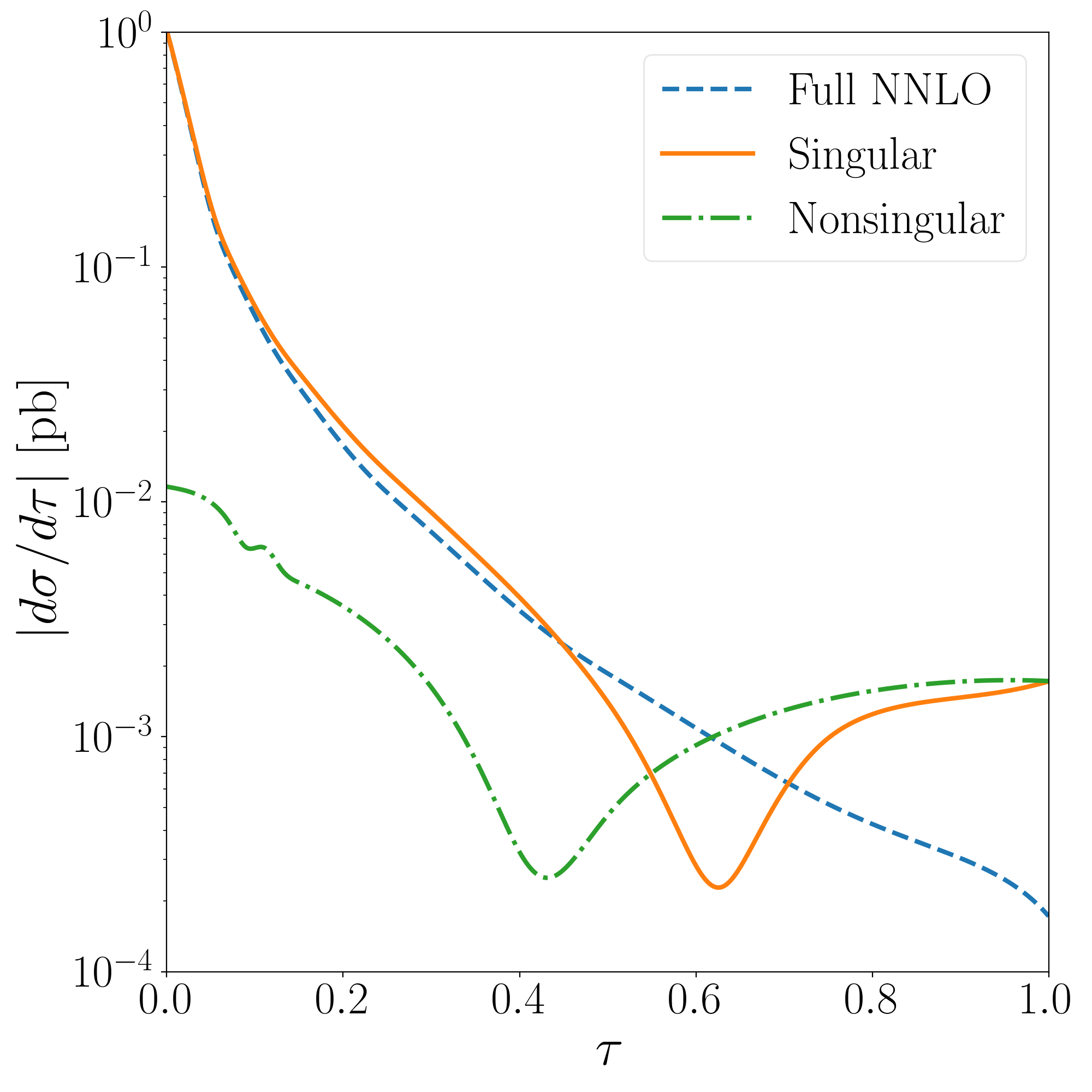
Figure 5: Comparison between the fixed-order distribution (Full NNLO), the absolute value of the expansion of the resummed contribution up to order $\alpha_{S}^{2}$ (Singular) and the absolute value of their difference (Nonsingular), as a function of $\tau$.

Appendix B Profile functions

The scales $\mu_{H}$, $\mu_{B}$, and $\mu_{S}$ at which the hard, beam and soft functions are evaluated are chosen using profile functions [88], following the prescriptions illustrated in Ref. [66]. Here we limit ourselves to explaining briefly the meaning of the four parameters on which they depend, namely $y_{0}$, $x_{1}$, $x_{2}$, and $x_{4}$, and how we set them. According to those prescriptions, the hard scale is kept fixed to $\mu_{H}=Q=M_{4\ell}$, while the beam and soft scales are run to resum the large logarithms. If we define a dimensionless

$$\tau=\frac{\mathcal{T}_{0}}{Q}\,,$$ (18)

in the region where $2y_{0}/Q<\tau<x_{1}$, the scales are chosen canonically, namely

$$\mu_{B}=\sqrt{\mathcal{T}_{0}Q}\qquad\mu_{S}=\mathcal{T}_{0}\,.$$ (19)

For $\tau<2y_{0}/Q$ the beam and soft scales are modified in a continuous way, so that, for $\tau\rightarrow 0$,

$$\mu_{B}\rightarrow\sqrt{y_{0}Q}\qquad\mu_{S}\rightarrow y_{0}\,.$$ (20)

This prevents the scales from reaching nonperturbative values, where the resummation framework breaks down. For this process we maintain the choice made in Ref. [66] and set

$$y_{0}=2.5\,\mathrm{GeV}\,.$$ (21)

At the opposite end of the spectrum, for $\tau>x_{3}$ the resummation must be switched off in order to recover the fixed-order result. This is achieved by setting

$$\mu_{B}=\mu_{S}=Q\,.$$ (22)

The parameter $x_{2}$ is used to choose how we turn off the resummation, usually picking it as the middle point between $x_{1}$ and $x_{3}$. In order to set the values for $x_{1}$ and $x_{3}$ we look at Fig. 5, where we compare the fixed-order distribution (Full NNLO), the absolute value of the expansion of the resummed contribution up to $\mathcal{O}(\alpha_{S}^{2})$ (Singular) and the absolute value of their difference (Nonsingular). We observe that the first two curves almost overlap in the region where $\tau\lesssim 0.2$ and that the nonsingular contribution becomes important at $\tau\approx 0.6$. Based on these considerations we choose the values

$$\{x_{1},x_{2},x_{3}\}=\{0.2,0.4,0.6\}\,.$$ (23)

References

- [1] G. Aad, et al., Measurement of the production cross section and limits on anomalous neutral triple gauge couplings in proton-proton collisions at TeV with the ATLAS detector, Phys. Rev. Lett. 108 (2012) 041804. arXiv:1110.5016, doi:10.1103/PhysRevLett.108.041804.
- [2] G. Aad, et al., Measurement of production in collisions at TeV and limits on anomalous and couplings with the ATLAS detector, JHEP 03 (2013) 128. arXiv:1211.6096, doi:10.1007/JHEP03(2013)128.
- [3] S. Chatrchyan, et al., Observation of Z Decays to Four Leptons with the CMS Detector at the LHC, JHEP 12 (2012) 034. arXiv:1210.3844, doi:10.1007/JHEP12(2012)034.
- [4] S. Chatrchyan, et al., Measurement of the production cross section and search for anomalous couplings in 2l2l’ final states in collisions at TeV, JHEP 01 (2013) 063. arXiv:1211.4890, doi:10.1007/JHEP01(2013)063.
- [5] G. Aad, et al., Measurements of four-lepton production in collisions at 8 TeV with the ATLAS detector, Phys. Lett. B753 (2016) 552–572. arXiv:1509.07844, doi:10.1016/j.physletb.2015.12.048.
- [6] M. Aaboud, et al., Measurement of the production cross section in proton-proton collisions at 8 TeV using the and channels with the ATLAS detector, JHEP 01 (2017) 099. arXiv:1610.07585, doi:10.1007/JHEP01(2017)099.
- [7] S. Chatrchyan, et al., Measurement of and Production Cross Sections in Collisions at , Phys. Lett. B 721 (2013) 190–211. arXiv:1301.4698, doi:10.1016/j.physletb.2013.03.027.
- [8] V. Khachatryan, et al., Measurement of the production cross section and constraints on anomalous triple gauge couplings in four-lepton final states at 8 TeV, Phys. Lett. B740 (2015) 250–272. arXiv:1406.0113, doi:10.1016/j.physletb.2014.11.059.
- [9] V. Khachatryan, et al., Measurements of the production cross sections in the channel in proton–proton collisions at and and combined constraints on triple gauge couplings, Eur. Phys. J. C 75 (10) (2015) 511. arXiv:1503.05467, doi:10.1140/epjc/s10052-015-3706-0.
- [10] G. Aad, et al., Measurement of the Production Cross Section in Collisions at = 13 TeV with the ATLAS Detector, Phys. Rev. Lett. 116 (10) (2016) 101801. arXiv:1512.05314, doi:10.1103/PhysRevLett.116.101801.
- [11] M. Aaboud, et al., cross-section measurements and search for anomalous triple gauge couplings in 13 TeV collisions with the ATLAS detector, Phys. Rev. D 97 (3) (2018) 032005. arXiv:1709.07703, doi:10.1103/PhysRevD.97.032005.
- [12] M. Aaboud, et al., Measurement of the four-lepton invariant mass spectrum in 13 TeV proton-proton collisions with the ATLAS detector, JHEP 04 (2019) 048. arXiv:1902.05892, doi:10.1007/JHEP04(2019)048.
- [13] M. Aaboud, et al., Measurement of production in the final state with the ATLAS detector in collisions at TeV, JHEP 10 (2019) 127. arXiv:1905.07163, doi:10.1007/JHEP10(2019)127.
- [14] V. Khachatryan, et al., Measurement of the ZZ production cross section and Z branching fraction in pp collisions at =13 TeV, Phys. Lett. B 763 (2016) 280–303, [Erratum: Phys.Lett.B 772, 884–884 (2017)]. arXiv:1607.08834, doi:10.1016/j.physletb.2016.10.054.
- [15] A. M. Sirunyan, et al., Measurements of the production cross section and the branching fraction, and constraints on anomalous triple gauge couplings at , Eur. Phys. J. C 78 (2018) 165, [Erratum: Eur.Phys.J.C 78, 515 (2018)]. arXiv:1709.08601, doi:10.1140/epjc/s10052-018-5567-9.
- [16] A. M. Sirunyan, et al., Measurements of production cross sections and constraints on anomalous triple gauge couplings at , Eur. Phys. J. C 81 (3) (2021) 200. arXiv:2009.01186, doi:10.1140/epjc/s10052-020-08817-8.
- [17] G. Aad, et al., Observation of a new particle in the search for the Standard Model Higgs boson with the ATLAS detector at the LHC, Phys. Lett. B 716 (2012) 1–29. arXiv:1207.7214, doi:10.1016/j.physletb.2012.08.020.
- [18] G. Aad, et al., Measurements of Higgs boson production and couplings in the four-lepton channel in pp collisions at center-of-mass energies of 7 and 8 TeV with the ATLAS detector, Phys. Rev. D91 (1) (2015) 012006. arXiv:1408.5191, doi:10.1103/PhysRevD.91.012006.
- [19] G. Aad, et al., Constraints on the off-shell Higgs boson signal strength in the high-mass and final states with the ATLAS detector, Eur. Phys. J. C75 (7) (2015) 335. arXiv:1503.01060, doi:10.1140/epjc/s10052-015-3542-2.
- [20] M. Aaboud, et al., Constraints on off-shell Higgs boson production and the Higgs boson total width in and final states with the ATLAS detector, Phys. Lett. B786 (2018) 223–244. arXiv:1808.01191, doi:10.1016/j.physletb.2018.09.048.
- [21] G. Aad, et al., Measurements of the Higgs boson inclusive and differential fiducial cross sections in the 4 decay channel at = 13 TeV, Eur. Phys. J. C 80 (10) (2020) 942. arXiv:2004.03969, doi:10.1140/epjc/s10052-020-8223-0.
- [22] S. Chatrchyan, et al., Observation of a New Boson at a Mass of 125 GeV with the CMS Experiment at the LHC, Phys. Lett. B 716 (2012) 30–61. arXiv:1207.7235, doi:10.1016/j.physletb.2012.08.021.
- [23] S. Chatrchyan, et al., Measurement of the properties of a Higgs boson in the four-lepton final state, Phys. Rev. D89 (9) (2014) 092007. arXiv:1312.5353, doi:10.1103/PhysRevD.89.092007.
- [24] V. Khachatryan, et al., Constraints on the Higgs boson width from off-shell production and decay to Z-boson pairs, Phys. Lett. B 736 (2014) 64–85. arXiv:1405.3455, doi:10.1016/j.physletb.2014.06.077.
- [25] V. Khachatryan, et al., Limits on the Higgs boson lifetime and width from its decay to four charged leptons, Phys. Rev. D 92 (7) (2015) 072010. arXiv:1507.06656, doi:10.1103/PhysRevD.92.072010.
- [26] V. Khachatryan, et al., Search for Higgs boson off-shell production in proton-proton collisions at 7 and 8 TeV and derivation of constraints on its total decay width, JHEP 09 (2016) 051. arXiv:1605.02329, doi:10.1007/JHEP09(2016)051.
- [27] A. M. Sirunyan, et al., Constraints on anomalous Higgs boson couplings using production and decay information in the four-lepton final state, Phys. Lett. B 775 (2017) 1–24. arXiv:1707.00541, doi:10.1016/j.physletb.2017.10.021.
- [28] A. M. Sirunyan, et al., Measurements of the Higgs boson width and anomalous couplings from on-shell and off-shell production in the four-lepton final state, Phys. Rev. D 99 (11) (2019) 112003. arXiv:1901.00174, doi:10.1103/PhysRevD.99.112003.
- [29] B. Mele, P. Nason, G. Ridolfi, QCD radiative corrections to Z boson pair production in hadronic collisions, Nucl. Phys. B357 (1991) 409–438. doi:10.1016/0550-3213(91)90475-D.
- [30] J. Ohnemus, J. Owens, An Order calculation of hadronic production, Phys. Rev. D43 (1991) 3626–3639. doi:10.1103/PhysRevD.43.3626.
- [31] J. Ohnemus, Hadronic , , and production with QCD corrections and leptonic decays, Phys. Rev. D50 (1994) 1931–1945. arXiv:hep-ph/9403331, doi:10.1103/PhysRevD.50.1931.
- [32] L. J. Dixon, Z. Kunszt, A. Signer, Vector boson pair production in hadronic collisions at order : Lepton correlations and anomalous couplings, Phys. Rev. D60 (1999) 114037. arXiv:hep-ph/9907305, doi:10.1103/PhysRevD.60.114037.
- [33] J. M. Campbell, R. K. Ellis, An Update on vector boson pair production at hadron colliders, Phys. Rev. D60 (1999) 113006. arXiv:hep-ph/9905386, doi:10.1103/PhysRevD.60.113006.
- [34] L. J. Dixon, Z. Kunszt, A. Signer, Helicity amplitudes for O() production of , , , , or pairs at hadron colliders, Nucl. Phys. B531 (1998) 3–23. arXiv:hep-ph/9803250, doi:10.1016/S0550-3213(98)00421-0.
- [35] E. Accomando, A. Denner, A. Kaiser, Logarithmic electroweak corrections to gauge-boson pair production at the LHC, Nucl. Phys. B706 (2005) 325–371. arXiv:hep-ph/0409247, doi:10.1016/j.nuclphysb.2004.11.019.
- [36] A. Bierweiler, T. Kasprzik, J. H. Kühn, Vector-boson pair production at the LHC to accuracy, JHEP 1312 (2013) 071. arXiv:1305.5402, doi:10.1007/JHEP12(2013)071.
- [37] J. Baglio, L. D. Ninh, M. M. Weber, Massive gauge boson pair production at the LHC: a next-to-leading order story, Phys. Rev. D88 (2013) 113005. arXiv:1307.4331, doi:10.1103/PhysRevD.88.113005.
- [38] B. Biedermann, A. Denner, S. Dittmaier, L. Hofer, B. Jäger, Electroweak corrections to at the LHC: a Higgs background study, Phys. Rev. Lett. 116 (16) (2016) 161803. arXiv:1601.07787, doi:10.1103/PhysRevLett.116.161803.
- [39] B. Biedermann, A. Denner, S. Dittmaier, L. Hofer, B. Jäger, Next-to-leading-order electroweak corrections to the production of four charged leptons at the LHC, JHEP 01 (2017) 033. arXiv:1611.05338, doi:10.1007/JHEP01(2017)033.
- [40] S. Kallweit, J. M. Lindert, S. Pozzorini, M. Schönherr, NLO QCD+EW predictions for diboson signatures at the LHC, JHEP 11 (2017) 120. arXiv:1705.00598, doi:10.1007/JHEP11(2017)120.
- [41] M. Chiesa, A. Denner, J.-N. Lang, Anomalous triple-gauge-boson interactions in vector-boson pair production with RECOLA2, Eur. Phys. J. C78 (6) (2018) 467. arXiv:1804.01477, doi:10.1140/epjc/s10052-018-5949-z.
- [42] F. Cascioli, T. Gehrmann, M. Grazzini, S. Kallweit, P. Maierhöfer, A. von Manteuffel, S. Pozzorini, D. Rathlev, L. Tancredi, E. Weihs, production at hadron colliders in NNLO QCD, Phys. Lett. B735 (2014) 311–313. arXiv:1405.2219, doi:10.1016/j.physletb.2014.06.056.
- [43] G. Heinrich, S. Jahn, S. P. Jones, M. Kerner, J. Pires, NNLO predictions for Z-boson pair production at the LHC, JHEP 03 (2018) 142. arXiv:1710.06294, doi:10.1007/JHEP03(2018)142.
- [44] M. Grazzini, S. Kallweit, D. Rathlev, ZZ production at the LHC: fiducial cross sections and distributions in NNLO QCD, Phys. Lett. B750 (2015) 407–410. arXiv:1507.06257, doi:10.1016/j.physletb.2015.09.055.
- [45] S. Kallweit, M. Wiesemann, production at the LHC: NNLO predictions for and signatures, Phys. Lett. B786 (2018) 382–389. arXiv:1806.05941, doi:10.1016/j.physletb.2018.10.016.
- [46] M. Grazzini, S. Kallweit, J. M. Lindert, S. Pozzorini, M. Wiesemann, NNLO QCD + NLO EW with Matrix+OpenLoops: precise predictions for vector-boson pair production, JHEP 02 (2020) 087. arXiv:1912.00068, doi:10.1007/JHEP02(2020)087.
- [47] F. Caola, K. Melnikov, R. Röntsch, L. Tancredi, QCD corrections to ZZ production in gluon fusion at the LHC, Phys. Rev. D92 (9) (2015) 094028. arXiv:1509.06734, doi:10.1103/PhysRevD.92.094028.
- [48] F. Caola, M. Dowling, K. Melnikov, R. Röntsch, L. Tancredi, QCD corrections to vector boson pair production in gluon fusion including interference effects with off-shell Higgs at the LHC, JHEP 07 (2016) 087. arXiv:1605.04610, doi:10.1007/JHEP07(2016)087.
- [49] M. Grazzini, S. Kallweit, M. Wiesemann, J. Y. Yook, production at the LHC: NLO QCD corrections to the loop-induced gluon fusion channel, JHEP 03 (2019) 070. arXiv:1811.09593, doi:10.1007/JHEP03(2019)070.
- [50] M. Grazzini, S. Kallweit, M. Wiesemann, J. Y. Yook, Four lepton production in gluon fusion: off-shell Higgs effects in NLO QCD, arXiv:2102.08344.
- [51] T. Melia, P. Nason, R. Röntsch, G. Zanderighi, W+W-, WZ and ZZ production in the POWHEG BOX, JHEP 11 (2011) 078. arXiv:1107.5051, doi:10.1007/JHEP11(2011)078.
- [52] P. Nason, G. Zanderighi, , and production in the POWHEG-BOX-V2, Eur. Phys. J. C 74 (1) (2014) 2702. arXiv:1311.1365, doi:10.1140/epjc/s10052-013-2702-5.
- [53] M. Chiesa, C. Oleari, E. Re, NLO QCD+NLO EW corrections to diboson production matched to parton shower, Eur. Phys. J. C 80 (9) (2020) 849. arXiv:2005.12146, doi:10.1140/epjc/s10052-020-8419-3.
- [54] S. Alioli, F. Caola, G. Luisoni, R. Röntsch, ZZ production in gluon fusion at NLO matched to parton-shower, Phys. Rev. D 95 (3) (2017) 034042. arXiv:1609.09719, doi:10.1103/PhysRevD.95.034042.
- [55] S. Alioli, S. Ferrario Ravasio, J. M. Lindert, R. Röntsch, Four-lepton production in gluon fusion at NLO matched to parton showers, arXiv:2102.07783.
- [56] K. Hamilton, P. Nason, E. Re, G. Zanderighi, NNLOPS simulation of Higgs boson production, JHEP 1310 (2013) 222. arXiv:1309.0017, doi:10.1007/JHEP10(2013)222.
- [57] S. Alioli, C. W. Bauer, C. Berggren, A. Hornig, F. J. Tackmann, et al., Combining Higher-Order Resummation with Multiple NLO Calculations and Parton Showers in GENEVA, JHEP 1309 (2013) 120. arXiv:1211.7049, doi:10.1007/JHEP09(2013)120.
- [58] S. Alioli, C. W. Bauer, C. Berggren, F. J. Tackmann, J. R. Walsh, et al., Matching Fully Differential NNLO Calculations and Parton Showers, JHEP 1406 (2014) 089. arXiv:1311.0286, doi:10.1007/JHEP06(2014)089.
- [59] S. Alioli, C. W. Bauer, C. Berggren, F. J. Tackmann, J. R. Walsh, Drell-Yan production at NNLL’+NNLO matched to parton showers, Phys. Rev. D92 (9) (2015) 094020. arXiv:1508.01475, doi:10.1103/PhysRevD.92.094020.
- [60] S. Höche, Y. Li, S. Prestel, Drell-Yan lepton pair production at NNLO QCD with parton showers, Phys. Rev. D 91 (7) (2015) 074015. arXiv:1405.3607, doi:10.1103/PhysRevD.91.074015.
- [61] S. Höche, Y. Li, S. Prestel, Higgs-boson production through gluon fusion at NNLO QCD with parton showers, Phys. Rev. D 90 (5) (2014) 054011. arXiv:1407.3773, doi:10.1103/PhysRevD.90.054011.
- [62] P. F. Monni, P. Nason, E. Re, M. Wiesemann, G. Zanderighi, MiNNLOPS: a new method to match NNLO QCD to parton showers, JHEP 05 (2020) 143. arXiv:1908.06987, doi:10.1007/JHEP05(2020)143.
- [63] P. F. Monni, E. Re, M. Wiesemann, MiNNLO: optimizing hadronic processes, Eur. Phys. J. C 80 (11) (2020) 1075. arXiv:2006.04133, doi:10.1140/epjc/s10052-020-08658-5.
- [64] S. Alioli, C. W. Bauer, A. Broggio, A. Gavardi, S. Kallweit, M. A. Lim, R. Nagar, D. Napoletano, L. Rottoli, Matching NNLO to parton shower using N3LL colour-singlet transverse momentum resummation in GENEVA, arXiv:2102.08390.
- [65] S. Alioli, A. Broggio, S. Kallweit, M. A. Lim, L. Rottoli, Higgsstrahlung at NNLL’NNLO matched to parton showers in GENEVA, Phys. Rev. D 100 (9) (2019) 096016. arXiv:1909.02026, doi:10.1103/PhysRevD.100.096016.
- [66] S. Alioli, A. Broggio, A. Gavardi, S. Kallweit, M. A. Lim, R. Nagar, D. Napoletano, L. Rottoli, Precise predictions for photon pair production matched to parton showers in GENEVA, JHEP 04 (2021) 041. arXiv:2010.10498, doi:10.1007/JHEP04(2021)041.
- [67] S. Alioli, A. Broggio, A. Gavardi, S. Kallweit, M. A. Lim, R. Nagar, D. Napoletano, L. Rottoli, Resummed predictions for hadronic Higgs boson decays, arXiv:2009.13533.
- [68] E. Re, M. Wiesemann, G. Zanderighi, NNLOPS accurate predictions for production, JHEP 12 (2018) 121. arXiv:1805.09857, doi:10.1007/JHEP12(2018)121.
- [69] M. Grazzini, S. Kallweit, S. Pozzorini, D. Rathlev, M. Wiesemann, production at the LHC: fiducial cross sections and distributions in NNLO QCD, JHEP 08 (2016) 140. arXiv:1605.02716, doi:10.1007/JHEP08(2016)140.
- [70] Munich is the abbreviation of “MUlti-chaNnel Integrator at Swiss (CH) precision”—an automated parton level NLO generator by S. Kallweit. In preparation.
- [71] S. Frixione, P. Nason, C. Oleari, Matching NLO QCD computations with Parton Shower simulations: the POWHEG method, JHEP 11 (2007) 070. arXiv:0709.2092, doi:10.1088/1126-6708/2007/11/070.
- [72] R. Kelley, M. D. Schwartz, R. M. Schabinger, H. X. Zhu, The two-loop hemisphere soft function, Phys. Rev. D84 (2011) 045022. arXiv:1105.3676, doi:10.1103/PhysRevD.84.045022.
- [73] P. F. Monni, T. Gehrmann, G. Luisoni, Two-Loop Soft Corrections and Resummation of the Thrust Distribution in the Dijet Region, JHEP 08 (2011) 010. arXiv:1105.4560, doi:10.1007/JHEP08(2011)010.
- [74] J. R. Gaunt, M. Stahlhofen, F. J. Tackmann, The Quark Beam Function at Two Loops, JHEP 04 (2014) 113. arXiv:1401.5478, doi:10.1007/JHEP04(2014)113.
- [75] A. Idilbi, X.-d. Ji, F. Yuan, Resummation of threshold logarithms in effective field theory for DIS, Drell-Yan and Higgs production, Nucl. Phys. B753 (2006) 42–68. arXiv:hep-ph/0605068, doi:10.1016/j.nuclphysb.2006.07.002.
- [76] T. Becher, M. Neubert, B. D. Pecjak, Factorization and Momentum-Space Resummation in Deep-Inelastic Scattering, JHEP 01 (2007) 076. arXiv:hep-ph/0607228, doi:10.1088/1126-6708/2007/01/076.
- [77] A. Hornig, C. Lee, I. W. Stewart, J. R. Walsh, S. Zuberi, Non-global Structure of the Dijet Soft Function, JHEP 08 (2011) 054. arXiv:1105.4628, doi:10.1007/JHEP08(2011)054.
- [78] D. Kang, O. Z. Labun, C. Lee, Equality of hemisphere soft functions for , DIS and collisions at , Phys. Lett. B 748 (2015) 45–54. arXiv:1504.04006, doi:10.1016/j.physletb.2015.06.057.
- [79] J. Gaunt, M. Stahlhofen, F. J. Tackmann, J. R. Walsh, N-jettiness Subtractions for NNLO QCD CalculationsarXiv:1505.04794.
- [80] F. Caola, J. M. Henn, K. Melnikov, A. V. Smirnov, V. A. Smirnov, Two-loop helicity amplitudes for the production of two off-shell electroweak bosons in quark-antiquark collisions, JHEP 1411 (2014) 041. arXiv:1408.6409, doi:10.1007/JHEP11(2014)041.
- [81] T. Gehrmann, A. von Manteuffel, L. Tancredi, The two-loop helicity amplitudes for leptons, JHEP 09 (2015) 128. arXiv:1503.04812, doi:10.1007/JHEP09(2015)128.
- [82] The VVamp project, by T. Gehrmann, A. von Manteuffel, and L. Tancredi, is publicly available at http://vvamp.hepforge.org.
- [83] F. Buccioni, J.-N. Lang, J. M. Lindert, P. Maierhöfer, S. Pozzorini, H. Zhang, M. F. Zoller, OpenLoops 2arXiv:1907.13071.
- [84] F. Cascioli, P. Maierhöfer, S. Pozzorini, Scattering Amplitudes with Open Loops, Phys. Rev. Lett. 108 (2012) 111601. arXiv:1111.5206, doi:10.1103/PhysRevLett.108.111601.
- [85] F. Buccioni, S. Pozzorini, M. Zoller, On-the-fly reduction of open loops, Eur. Phys. J. C 78 (1) (2018) 70. arXiv:1710.11452, doi:10.1140/epjc/s10052-018-5562-1.
- [86] R. D. Ball, et al., Parton distributions from high-precision collider data, Eur. Phys. J. C 77 (10) (2017) 663. arXiv:1706.00428, doi:10.1140/epjc/s10052-017-5199-5.
- [87] A. Buckley, J. Ferrando, S. Lloyd, K. Nordström, B. Page, M. Rüfenacht, M. Schönherr, G. Watt, LHAPDF6: parton density access in the LHC precision era, Eur. Phys. J. C75 (3) (2015) 132. arXiv:1412.7420, doi:10.1140/epjc/s10052-015-3318-8.
- [88] I. W. Stewart, F. J. Tackmann, J. R. Walsh, S. Zuberi, Jet resummation in Higgs production at , Phys. Rev. D 89 (2014) 054001. arXiv:1307.1808, doi:10.1103/PhysRevD.89.054001.