Expected Value of Communication
for Planning in Ad Hoc Teamworks

Abstract

A desirable goal for autonomous agents is to be able to coordinate on the fly with previously unknown teammates. Known as “ad hoc teamwork”, enabling such a capability has been receiving increasing attention in the research community. One of the central challenges in ad hoc teamwork is quickly recognizing the current plans of other agents and planning accordingly. In this paper, we focus on the scenario in which teammates can communicate with one another, but only at a cost. Thus, they must carefully balance plan recognition based on observations vs. that based on communication.

This paper proposes a new metric for evaluating how similar are two policies that a teammate may be following - the Expected Divergence Point (edp). We then present a novel planning algorithm for ad hoc teamwork, determining which query to ask and planning accordingly. We demonstrate the effectiveness of this algorithm in a range of increasingly general communication in ad hoc teamwork problems.

Introduction

Modern autonomous agents are often required to solve complex tasks in challenging settings, and to do so as part of a team. For example, service robots have been deployed in hospitals to assist medical teams in the recent pandemic outbreak. The coordination strategy of such robots cannot always be fixed a priori, as it may involve previously unmet teammates that can have a variety of behaviors. These robots will only be effective if they are able to work together with other teammates without the need for coordination strategies provided in advance (Cakmak and Thomaz 2012). This motivation is the basis for ad hoc teamwork, which is defined from the perspective of a single agent, the Ego Agent, that needs to collaborate with teammates without any pre-coordination (Stone et al. 2010; Albrecht and Stone 2018). Without pre-coordination, only very limited knowledge about any teammate, such as that they have limited rationality or what their potential goals are, is available. An important capability of ad hoc teamwork is plan recognition of teammates, as their goals and plans can affect the goals and plans of the ego agent. Inferring these goals is not trivial, as the teammates may not provide any information about their policies, and the execution of their plan might be ambiguous. Hence, it is up to the ego agent to disambiguate between potential goals. The first contribution of this paper is a metric to evaluate ambiguity between two potential teammate policies by quantifying the number of steps a teammate will take (in expectation) until it executes an action that is consistent with only one of the two policies. We show how this edp metric can be computed in practice using a Bellman update.

In addition to applying a reasoning process to independently infer the goal of its teammate, the ego agent can also directly communicate with that teammate to gain information faster than it would get by just observing. However, if such a communication channel is available, it can come with a cost, and the ego agent should appropriately decide when and what to communicate. For example, if the previously described medical robot can fetch different tools for a physician in a hospital, the physician would generally prefer to avoid the additional cognitive load of communicating with the robot, but may be willing to answer an occasional question so that it can be a better collaborator. We refer to this setting where the ego agent can leverage communication to collaborate with little to no knowledge about its teammate as Communication in Ad hoc Teamwork, or cat (Mirsky et al. 2020). The second contribution of this paper is using edp in a novel planning algorithm for ad hoc teamwork that reasons about the value of querying and chooses when and what to query about in the presence of previously unmet teammates.

Lastly, this paper presents empirical results showing the performance of the new edp-based algorithm in these complex settings, showing that it outperforms existing heuristics in terms of total number of steps required for the team to reach its goal. Moreover, the additional computations required of the edp-based algorithm can mostly take place prior to the execution, and hence its online execution time does not differ significantly from simpler heuristics.

Related Work

There is a vast literature on reasoning about teammates with unknown goals (Fern et al. 2007; Albrecht and Stone 2018) and on communication between artificial agents (Cohen, Levesque, and Smith 1997; Decker 1987; Pynadath and Tambe 2002), but significantly less works discuss the intersection between the two, and almost no work in an ad hoc teamwork setting. Goldman and Zilberstein (2004) formalized the problem of collaborative communicating agents as a decentralized POMDP with communication (DEC-POMDP-com). Communication in Ad-Hoc Teamwork (cat) is a related problem that shares some assumptions with DEC-POMDP-com:

• All teammates strive to be collaborative.

• The agents have a predefined communication protocol available that cannot be modified during execution.

• The policies of the ego agent’s teammates are set and cannot be changed. This assumption does not mean that agents cannot react to other agents and their actions, but rather that such reactions are consistent as determined by the set policy.

However, these two problems make different assumptions that separate them. DEC-POMDP-com uses a single model jointly representing all plans, and this model is collaboratively controlled by multiple agents. cat, on the other hand, is set from the perspective of one agent with a limited knowledge about its teammates’ policies (such as that all agents share the same goal and strive to be collaborative) and thus it cannot plan a priori how it might affect these teammates (Stone et al. 2013; Ravula, Alkoby, and Stone 2019).

In recent years there have been some works that considered communication in ad hoc teamwork (Barrett et al. 2014; Chakraborty et al. 2017). These works suggested algorithms for ad hoc teamwork, where teammates either share a common communication protocol, or can test the policies of the teammates on the fly (e.g. by probing). These works are situated in a very restrictive multi-agent setting, namely a multi-arm bandit, where each task consists of a single choice of which arm to pull. Another recent work on multi-agent sequential plans proposed an Inverse Reinforcement Learning technique to infer teammates’ goals on the fly, but it assumes that no explicit communication is available (Wang et al. 2020).

With recent developments in deep learning, several works were proposed for a sub-area of multi-agent systems, where agents share information using learned communication protocols (Hernandez-Leal, Kartal, and Taylor 2019; Mordatch and Abbeel 2018; Foerster et al. 2016). These works make several assumptions not used in this work: that the agents can learn new communication skills, and that an agent can train with its teammates before execution. An exception to that is the work of Van Zoelen et al. (2020) where an agent learns to communicate both beliefs and goals, and applies this knowledge within human-agent teams. Their work differs from ours in the type of communication they allow.

Several other metrics have been proposed in the past to evaluate the ambiguity of a domain and a plan. Worst Case Distinctiveness (wcd) is defined as the longest prefix that any two plans for different goals share (Keren, Gal, and Karpas 2014). Expected Case Distinctiveness (ecd) weighs the length of a path to a goal by the probability of an agent choosing that goal and takes the sum of all the weighted path lengths (Wayllace, Hou, and Yeoh 2017). Both these works only evaluate the distinctiveness between two goals with specific assumptions about how an agent plans, while edp evaluate the expected case distinctiveness for any pair of policies, which may or may not be policies to achieve two different goals.

A specific type of cat scenarios refers to tasks where a single agent reasons about the sequential plans of other agents, and can gain additional information by querying its teammates or by changing the environment (Mirsky et al. 2018, 2020; Shvo and McIlraith 2020). In this paper, we focus on a specific variant of this problem known as Sequential One-shot Multi-Agent Limited Inquiry cat scenario, or somali cat (Mirsky et al. 2020). Consider the use case of a service robot that is stationed in a hospital, that mainly has to retrieve supplies for physicians or nurses, and has two main goals to balance: understanding the task-specific goals of its human teammates, and understanding when it is appropriate to ask questions over acting autonomously. As the name somali cat implies, this scenario includes several additional assumptions: The task is episodic, one-shot, and requires a sequence of actions rather than a single action (like in the multi-armed bandit case); the environment is static, deterministic, and fully observable; the teammate is assumed to plan optimally, given that it is unaware of the ego agent’s plans or costs; and there is one communication channel, where the ego agent can query as an action, and if it does, the teammate will forgo its action to reply truthfully (the communication channel is noiseless). The definition of edp and the algorithm presented in this paper rely on this set of assumptions as well. While previous work by the authors in somali cat gave effective methods for determining when to ask a query (Mirsky et al. 2020), they did not provide a principled method for determining what to query. In this work, we extend previous methods with a principled technique for constructing a query.

Background

The notation and terminology we use in this paper is patterned closely after that of Albrecht and Stone (2017), extended to reason about communication between agents. We define a somali cat problem as a tuple $C=\langle S,A_{A},A_{T},T,C\rangle$ where $S$ is the set of states, $A_{A}$ is the set of actions the ad-hoc agent can execute, $A_{T}$ is the set of actions the teammate can execute, $T$ is the transition function $T:S\times A_{A}\times A_{T}\times S\to[0,1]$, and $C:A_{A}\times A_{T}\rightarrow\mathbb{R}$ maps joint actions to a cost. Specifically, $A_{A}=O_{A}\cup Q$ consists of a set of actions $O_{A}$ that can change the state of the world, which we refer to as ontic actions, as defined in Muise et al. (2015), and a set of potential queries $Q$ it can ask. Similarly, $A_{T}=O_{T}\cup R$ is a set of ontic actions that the teammate can execute $O_{T}$ and the set of possible responses $R$ to the ego agent’s query. Actions in $O_{i}$ can be selected independently from the decisions of other agents, but if the ego agent chooses to query the teammate at timestep $t$, then the action of the ego agent is some $q\in Q$ and the teammate’s action must be $r\in R$. In this case, if the ego agent queries, both agents forego the opportunity to select an ontic action; the ego agent uses an action to query and the teammate uses an action to respond. A policy $\pi$ for agent $i$ is a distribution over tuples of states and actions, such that $\pi_{i}(s,a)$ is the probability with which agent $A_{i}$ executes $a\in A_{i}$ in state $s\in S$. Policy $\pi_{i}$ induces a trajectory $Tr_{i}=\langle s^{0},a_{i}^{1},s^{1},a_{i}^{2},s^{2}...\rangle$. The cost of a joint policy execution is the accumulated cost of the constituent joint actions of the induced trajectories. For simplicity, in this work we assume that all ontic actions have a joint cost of 1. Queries and responses have different costs depending on their complexity.

Additional useful notation that will be used throughout this paper is the Uniformly-Random-Optimal Policy (or urop) $\hat{\pi}_{g}$, that denotes the policy that considers all plans that arrive at goal $g$ with minimal cost, samples uniformly at random from the set of these plans, and then chooses the first action of the sampled plan.

In order to ground $Q$ to a discrete, finite set of potential queries, we first need to define a goal of the teammate $g$ as the set of states in $S$ such that a set of desired properties holds (e.g., both the physician and the robot are in the right room). Given this definition, we can use a concrete set of queries $Q$ of the format: “Is your goal in $G$?” where $G$ is a subset of possible goals. This format of queries was chosen as it can replace any type of query that disambiguates between potential goals (e.g. “Is your goal on the right?”, “What are your next k actions?”), as long as we know how to map the query to the goals it can disambiguate.

Expected Divergence Point

The first major contribution of this paper is a formal way to quantify the ambiguity between two policies, based on the number of steps we expect to observe before we see an action that can only be explained by a plan that can be executed when following one policy, but not by a plan that follows the other policy. Consider 2 policies $\pi_{1},\pi_{2}$, and assume that policy $\pi_{2}$ was used to construct the trajectory $Tr_{2}$.

Definition 1.

The divergence point (dp) from $\pi_{1}$, or the minimal point in time such that we know $Tr_{2}$ was not produced by $\pi_{1}$, is defined as follows:

$$dp(\pi_{1}\mid Tr_{2})=min\{t\mid\pi_{1}(s_{t-1},a_{2}^{t})=0\}$$

Figure 1 shows an example in which the teammate is in the light gray tile $(4,3)$ and is marked using the robot image. The goal of this agent can either be $g_{1}$ or $g_{2}$ (dark gray tiles), and the policies $\hat{\pi}_{g_{1}}$ and $\hat{\pi}_{g_{2}}$ are the urops for $g_{1}$ and $g_{2}$ respectively. If an agent were to follow the path outlined in red starting at state $(4,3)$, then the $dp$ of this path with $\hat{\pi}_{g_{1}}$ would be 3 as the path diverges from $\hat{\pi}_{g_{1}}$ at timestep 3.

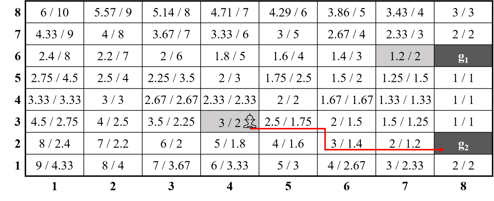
Figure 1: Various edp values in a grid world with two goals. Values are presented as $\textsc{edp}(s,\hat{\pi}_{g_{1}}|\hat{\pi}_{g_{2}})/\textsc{edp}(s,\hat{\pi}_{g_{2}}|\hat{\pi}_{g_{1}})$.

To account for stochastic policies, where a policy will generally produce more than one potential trajectory from a state, we introduce the expected divergence point that considers all possible trajectories constructed from $\pi_{2}$.

Definition 2.

The Expected Divergence Point (edp) of policy $\pi_{1}$ from $\pi_{2}$, starting from state $s$ is

$$\textsc{edp}(s,\pi_{1}\mid\pi_{2})=\mathbb{E}_{Tr_{2}}[dp(\pi_{1}\mid Tr_{2})]$$

Computing edp directly from this equation is non trivial. We therefore rewrite edp as the following Bellman update:

Theorem 1.

The Bellman update for edp of the policies $\pi_{1},\pi_{2}$, starting from state $s$ is:

$$\begin{split}\textsc{edp}&(s,\pi_{1}|\pi_{2})=[1-\sum\limits_{a\in A^{\prime}(s)}\pi_{2}(s,a)]+\\ &\sum\limits_{a\in A^{\prime}(s)}\pi_{2}(s,a)*\sum\limits_{s^{\prime}\in S}T(s,a,s^{\prime})[1+\textsc{edp}(s^{\prime},\pi_{1}|\pi_{2})]\end{split}$$ (1)

where $A^{\prime}(s)=\{a\in A|\pi_{1}(s,a)>0\}$.

Proof.

We first define $P(dp(\pi_{1}\mid Tr_{2})=n)$ to be the probability of seeing $n$ steps before observing an action that $\pi_{1}$ will not take in state $s_{n-1}$, assuming that $Tr_{2}$ is some trajectory sampled from $\pi_{2}$. Then edp can be written as:

$$\textsc{edp}(s,\pi_{1}\mid\pi_{2})=\sum\limits_{t=1}^{\infty}[P(dp(\pi_{1}\mid Tr_{2})=t)*t]$$ (2)

Next, we compute this probability as the joint probability of the $k$-th action in $\pi_{1}$ being different from $a_{2}^{k}$ for all $k<n$ and $\pi_{1}(s_{n-1},a_{1}^{n})=a_{2}^{n}$:

$$\begin{split}&P(dp(\pi_{1}\mid Tr_{2})=1)=P(\pi_{1}(s_{0},a_{2}^{1})=0),\\ &P(dp(\pi_{1}\mid Tr_{2})=2)=P(\pi_{1}(s_{0},a_{2}^{1})\neq 0)*P(\pi_{1}(s_{1},a_{2}^{2})=0),\\ &P(dp(\pi_{1}\mid Tr_{2})=3)=P(\pi_{1}(s_{0},a_{2}^{1})\neq 0)*P(\pi_{1}(s_{0},a_{2}^{2})\neq 0)*\\ &\qquad\qquad\qquad\qquad\qquad~{}~{}~{}~{}~{}~{}P(\pi_{1}(s_{1},a_{2}^{3})=0)\end{split}$$ (3)

and so on. Given these equations, we can rewrite the infinite summation in Equation 2:

$$\begin{split}\textsc{edp}&(s,\pi_{1}|\pi_{2})=\\ &P(\pi_{1}(s_{0},a_{2}^{1})=0)+\\ &2*P(\pi_{1}(s_{0},a_{2}^{1})\neq 0)*P(\pi_{1}(s_{1},a_{2}^{2})=0)+\\ &3*P(\pi_{1}(s_{0},a_{2}^{1})\neq 0)*P(\pi_{1}(s_{0},a_{2}^{2})\neq 0)*P(\pi_{1}(s_{1},a_{2}^{3})=0)+\ldots\end{split}$$

We can factor out a $P(\pi_{1}(s_{0},a_{1})\neq 0)$ from all of the first portion of the summation to get the following:

$$\begin{split}\textsc{edp}&(s,\pi_{1}|\pi_{2})=\\ &P(\pi_{1}(s_{0},a_{2}^{1})=0)+P(\pi_{1}(s_{0},a_{2}^{1})\neq 0)*\\ &[2*P(\pi_{1},a_{2}^{2}=0)+3*(\pi_{1}(s_{0},a_{2}^{2})\neq 0)*P(\pi_{1}(s_{1},a_{2}^{3})=0)+\ldots]\end{split}$$

In reverse to the transition from Equation 2 to Equation 3 and by using Bayes rule, the bracketed portion can be compiled back into an infinite sum:

$$\begin{split}\textsc{edp}&(s,\pi_{1}|\pi_{2})=\\ &P(\pi_{1}(s_{0},a^{1}_{2})=0)+P(\pi_{1}(s_{0},a^{1}_{2})\neq 0)*\\ &\sum\limits_{t=1}^{\infty}[(t+1)*P(dp(\pi_{1}\mid Tr_{2})=t+1\mid\pi_{1}(s_{0},a^{1}_{2})\neq 0)]\end{split}$$

We distribute the multiplication by $(t+1)$ inside the summation to arrive at the following:

$$\begin{split}\textsc{edp}&(s,\pi_{1}|\pi_{2})=\\ &P(\pi_{1}(s_{0},a_{2}^{1})=0)+P(\pi_{1}(s_{0},a_{2}^{1})\neq 0)*\\ &[\sum\limits_{t=1}^{\infty}(t*P(dp_{\pi_{1}}(Tr_{2})=t+1\mid\pi_{1}(s_{0},a_{2}^{1})\neq 0))+\\ &\sum\limits_{t=1}^{\infty}(P(dp_{\pi_{1}}(Tr_{2})=t+1\mid\pi_{1}(s_{0},a_{2}^{1})\neq 0))]\end{split}$$

The second summation simplifies to 1, while the first is equivalent to the edp at the following state. Using this knowledge we derive the following formula for edp:

$$\begin{split}\textsc{edp}&(s,\pi_{1}|\pi_{2})=\\ &P(\pi_{1}(s_{0},a_{2}^{1})=0)+P(\pi_{1}(s_{0},a^{2}_{1})\neq 0)*\\ &[\sum\limits_{s^{\prime}\in S}T(s,a_{2}^{0},s^{\prime})*(1+\textsc{edp}(s^{\prime},\pi_{1}|\pi_{2}))]\end{split}$$

Remember that the term $P(\pi_{1}(s_{0},a_{2}^{1})\neq 0)$ is the probability of sampling a first action in $Tr_{2}$ that will be the same as the action taken in $s_{0}$ according to $\pi_{1}$. Consider the set $A^{\prime}(s)=\{a\in A|\pi_{1}(s,a)>0\}$, and note that $P(\pi_{1}(s_{0},a_{2}^{1})\neq 0)$ is the same as $\sum\limits_{a\in A^{\prime}(s_{0})}\pi_{2}(s_{0},a)$. We therefore arrive at the Bellman update from Equation 1. ∎

There are a few things to note regarding edp. First, it is not a symmetric relation: $\textsc{edp}(s,\pi_{1}|\pi_{2})$ does not necessarily equal $\textsc{edp}(s,\pi_{2}|\pi_{1})$. For example, Figure 1 presents the value of $\textsc{edp}(s,\hat{\pi}_{g_{1}}|\hat{\pi}_{g_{2}})$ and the value of $\textsc{edp}(s,\hat{\pi}_{g_{2}}|\hat{\pi}_{g_{1}})$ side by side for each tile. In addition, neither of the edp values necessarily equals the ecd of this domain, as presented by Wayllace et al. (2017), where ecd estimates the probability of taking action $a$ in state $s$ as the normalized weighted probability of all goals for which $a$ is optimal from $s$. Consider tile $(7,6)$ which is colored in light gray. Assuming uniform probability over goals, the ecd when the teammate is in this state is $1.67$, a value distinct from both the edp values in this state, as well as from their average.

Next, we show how edp can be used to compute the timesteps in which the ego agent is expected to benefit from querying, and then how this information can be used by the ego agent for planning when and what to query.

Expected Zone of Querying

Previous work provided a means to reason about when to act in the environment and when to query, in the form of three different reasoning zones general to all somali cat domains (Mirsky et al. 2020). The zones that were defined with respect to querying are:

Zone of Information ($Z_{I}$)

given the location of the teammate and two of its possible goals $g_{1},g_{2}$, $Z_{I}$ is the interval from the beginning of the plan up to the worst case distinctiveness of $g_{1},g_{2}$ for recognizing the teammate’s goal, as defined by Keren et al. (2014).

Intuitively, these are the timesteps where the ego agent might gain information by querying about these goals.

Zone of Branching ($Z_{B}$)

given the location of the ego agent and two possible goals of the teammate, $Z_{B}$ is the interval from the worst case distinctiveness of $g_{1},g_{2}$ for recognizing the ego agent’s goal and up to the end of the episode. Intuitively, these are the timesteps where the ego agent might take a non-optimal action if it could not disambiguate between the two goals of its teammate.

Zone of Querying ($Z_{Q}$)

given the locations of the ego agent, the teammate, and two possible goals of the teammate, $Z_{Q}$ is the intersection of $Z_{I}$ and $Z_{B}$ for these goals, where there may be a positive value in querying about the two goals instead of acting. Intuitively, these are the timesteps where the ego agent cannot distinguish between the two possible goals of the teammate and it should take different actions in each case.

Consider the running example from Figure 1, and assume that this grid represents a maximal coverage task, where the agents need to go to different goals in order to cover as many goals as possible (Pita et al. 2008). Consider an ego agent with the aim to go to a different goal from its teammate which is in tile $(4,3)$. The Zone of Information which depends only on the behavior of the teammate, is $Z_{I}(\{g_{1},g_{2}\})=\{t\mid t\leq 5\}$, as 5 is the maximum number of steps that the teammate can take before its goal is disambiguated (e.g., if the agent moves east 4 times only its fifth action will disambiguate its goal). If the ego agent is in tile $(5,4)$, then $Z_{B}(\{g_{1},g_{2}\})=\{t\mid t\geq 4\}$ and hence $Z_{Q}(\{g_{1},g_{2}\})=\{4,5\}$. However, if the ego agent is in tile $(2,4)$, then $Z_{B}(\{g_{1},g_{2}\})=\{t\mid t\geq 7\}$, and hence in this case $Z_{Q}(\{g_{1},g_{2}\})=\emptyset$. These existing definitions of zones consider the worst case for disambiguating goals. However, the worst case might be highly uncommon, and planning when to query accordingly can induce high costs. Using edp, we now have the requirements to compute the expected case for disambiguation of goals. We introduce definitions for expected zones:

Definition 3.

The Expected Zone of Information $eZ_{I}$ given the location of the teammate and two goals $g_{1},g_{2}$, $eZ_{I}$ is the expected time period during which the teammate’s plan is ambiguous between $g_{1}$ and $g_{2}$:

$$eZ_{I}(s,g_{1}|g_{2})=\{t|t\leq\textsc{edp}(s,\hat{\pi}_{g_{1}}|\hat{\pi}_{g_{2}})\}$$

where the policies $\hat{\pi}_{g_{1}},\hat{\pi}_{g_{2}}$ are the urops of the teammate for goals $g_{1}$ and $g_{2}$ respectively.

Intuitively, $eZ_{I}$ for two goals is the set of timesteps where we don’t expect to see an action that can only be executed by $g_{1}$ but not by $g_{2}$. Similarly, $eZ_{B}$ for two goals is the set of all timesteps where we expect that the ego agent will take a non-optimal action if it does not have perfect knowledge about the teammate’s true goal.

Definition 4.

The Expected Zone of Branching for goals $g_{1},g_{2}$ is the expected time period where the ego agent can take an optimal action for $g_{2}$ without incurring additional cost if the teammate’s true goal is $g_{1}$:

$$eZ_{B}(s,g_{1}|g_{2})=\{t|t\geq\textsc{edp}(s,\hat{\pi}_{g_{2}}|\hat{\pi}_{g_{1}})\}$$

where the policies $\hat{\pi}_{g_{1}}$ and $\hat{\pi}_{g_{2}}$ are the urops of the ego agent for goals $g_{1}$ and $g_{2}$ respectively.

Definition 5.

The Expected Zone of Querying for goals $g_{1},g_{2}$ is the time period where the ego agent is expected to benefit from querying:

$$eZ_{Q}(s,g_{1}|g_{2})=eZ_{B}(s,g_{1}|g_{2})\cap eZ_{I}(s,g_{1}|g_{2})$$

In our empirical settings, we have control over the ego agent, and can therefore guarantee it will follow an optimal plan given its current knowledge about the teammate’s goal. In this case, we can use the original definition of $Z_{B}$ instead of $eZ_{B}$, as they are equivalent in this setting.

Using $eZ_{Q}$ for Planning

Next, we present a planning algorithm for the ego agent that uses the value of a query to minimize the expected cost of the chosen plan. In this planning process, there are two main problems that need to be solved: determining when to query and what to query. Using the definition of $Z_{Q}$, we can easily determine when querying would certainly be redundant, and respectively, when a query might be useful. Once we know that a query might be beneficial, we can use $eZ_{Q}$ to determine what to query exactly. Notice that the conclusion might still be not to query at all. For example, consider the maximal coverage example from Figure 1, where the teammate is in tile $(4,3)$, and the ego agent is in tile $(8,4)$. As the teammate can choose to move east, there is still ambiguity between $g_{1}$ and $g_{2}$ and the ego agent must choose between moving north or south - so according to $Z_{Q}$ the ego agent should query. However, if it highly unlikely that the teammate would go east, the expected gain from querying decreases significantly. Thus, even though $Z_{Q}$ is not empty, it is not a good strategy for the ego agent to query.

In this section, we discuss how to use the new $eZ_{Q}$ to compute the value of a specific query more accurately than proposed by previous approaches This information will be used in an algorithm for the ego agent that chooses the best query. The first step is calculating the edp for each pair of goals $g_{1}$ and $g_{2}$ and their corresponding urops $\hat{\pi}_{g_{1}}$ and $\hat{\pi}_{g_{2}}$. We use a modified version of the dynamic programming policy evaluation algorithm (Bellman 1966) applied on the bellman update presented in Equation 1 (additional details can be found in the Appendix. As this policy evaluation does not depend on the teammate’s actions, it can be done offline prior to the plan execution, as presented in Figure 1. Next, using these values, we can compute the value of a specific query.

Computing the Value of a Query

Given a somali cat domain $\langle S,A_{A},A_{T},T,C\rangle$, we want to quantify how much, in terms of expected plan cost, the ego agent can gain from asking a specific query. Therefore, we define the value of a query as follows:

Definition 6.

Value of a Query Let $q$ be a query with possible responses $R$, and $\mathcal{P}_{g}$ be the set of possible plans of both agents that arrive at goal $g$. Then the value of query $q$ is

$$V(q)=\mathbb{E}_{p\in\mathcal{P}_{g}}[cost(p)]-\sum\limits_{r\in R}P(r)*\mathbb{E}_{p\in\mathcal{P}_{g}}[cost(p)|r]$$ (4)

Computing the expected cost of this set of plans is non-trivial. We therefore define the following concept:

Definition 7.

The Marginal Cost of a plan $p$ in a somali cat domain with a goal $g$ ($MC_{g}(p)$) is the difference between the cost of $p$ and the cost of a minimal-cost plan that arrives at $g$.

We can replace $cost(p)$ in Equation 4 with $MC_{g}(p)$ to yield an equivalent formula that is easier to compute:

$$\begin{split}V&(q)=\\ &(\mathbb{E}_{p\in\mathcal{P}_{g}}[cost(p)]-c^{*}_{g})-(\sum\limits_{r\in R}P(r)*\mathbb{E}_{p\in\mathcal{P}_{g}}[cost(p)|r]-c^{*}_{g})=\\ &\mathbb{E}_{p\in\mathcal{P}_{g}}[MC_{g}(p)]-\sum\limits_{r\in R}P(r)*\mathbb{E}_{p\in\mathcal{P}_{g}}[MC_{g}(p)|r]\end{split}$$ (5)

where $c^{*}_{g}$ is the minimal cost of a plan that arrives at $g$.

In somali cat, $\mathbb{E}_{p\in\mathcal{P}_{g}}[MC_{g}(p)]$ at state $s$ is proportional to the number of timesteps in which the ego agent doesn’t know which ontic actions are optimal, or formally:

$$\mathbb{E}_{p\in\mathcal{P}_{g}}[MC_{g}(p)]\propto|\bigcup\limits_{g^{\prime}\in G}eZ_{Q}(s,g^{\prime}|g)|$$

In addition, notice that computing $V(q)$ using Equation 5 assumes that the goal of the teammate, $g$, is known. However, the ego agent does not know the true goal $g$ ahead of time, so we need to consider the expected value of a query for each possible goal of the teammate, or $\mathbb{E}_{g\in G}[V(q)|g]$.

Choosing What to Query

Our policy for determining whether or not to query at each timestep is shown in Algorithm 1. It takes as input the Zone of Querying for each pair of goals, $Z_{Q}$, the expected Zone of Querying $eZ_{Q}$, the current set of possible goals $G$, the ego agent’s current belief of the teammate’s goal $P$ and the current timestep $t$. First the algorithm checks if the current timestep is within a Zone of Querying of two goals or more. If not, then the agent knows of an optimal ontic action and no querying is required. Otherwise, we then find the best possible query given $eZ_{Q}$, and only ask this query if its value is greater than its cost.

Algorithm 1 Query Policy

procedure Query($Z_{Q}$ for each pair of goals, $eZ_{Q}$ for each pair of goals, $G$, $P$, current timestep $t$)

     if $\exists g_{1},g_{2}\in G\textit{ s.t. }t\in Z_{Q}(g_{1},g_{2}))$ then

         $query\leftarrow ChooseQuery(G,eZ_{Q},P)$

         if $value(query)-cost(query)>0$ then

              return $query$

         end if

     end if

     return No Query

end procedure

To optimize the expected value of a chosen query, we define a binary vector x for each possible query, such that $x_{i}$ is 1 if and only if $g_{i}$ is included in that query. We then optimize for the difference between the value of a query above and its cost over these vectors using a genetic algorithm. We use a population size of $50$ and optimize for $100$ generations. Members are selected using tournament selection, and then combined using crossover. Each bit in the two resulting members is mutated with probability $0.001$.

Experimental Setup

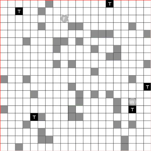
Figure 2: Example instance of the tool fetching domain. Workstations are shown by the grey boxes, toolboxes are shown by the black boxes with a T, the fetcher is shown as the gray circle labeled with an F, while the worker is shown as a gray circle labeled with a W.

Previous work in somali cat introduced an experimental domain known as the tool fetching domain (Mirsky et al. 2020). This domain consists of an ego agent, the fetcher, attempting to meet a teammate, the worker, at some workstation with a tool. The worker needs a specific tool depending on which station is its goal, and the worker’s goal and policy are unknown to the fetcher. It is the job of the fetcher to deduce the goal of the worker based on its actions, to pick up the correct tool from a toolbox and to bring it to the correct workstation. At each timestep, the agents can execute one ontic action each. In this work, the fetcher infers the worker’s true goal by setting a goal’s probability to zero and normalizing the belief distribution when observing a non-optimal action for that goal. Alternatively, the fetcher can query the worker with questions of the form “Is your goal one of the stations $g_{1},g_{2}...g_{N}$?”, where $g_{1},\ldots,g_{N}\subseteq G$ is a subset of all workstations, and the worker replies truthfully. All queries are assumed to have a cost identical to moving one step, regardless of the content of the query. To show the benefits of our algorithm, we introduce 3 generalizations to the tool fetching domain that make the planning problem for the ego agent more complex to solve.

Multiple $Z_{B}$s

We allow multiple toolboxes in the domain. Each toolbox contains a unique set of tools, and only one tool for each station is present in a domain. Including this generalization means that each pair of goals may have different $Z_{B}$ values, which makes determining query timing and content more challenging.

Non-uniform Probability

We allow non-uniform probability distributions for assigning the worker a goal. For instance, goals may be assigned with probability corresponding to the Boltzmann distribution over the negative of their distances. This modification means that the worker is more likely to have goals that are closer to it. Including this generalization means that querying about certain goals may be more valuable than others, and the fetcher will have to consider this distribution when deciding what to query about.

Cost Model

We allow for a more general cost model, where different queries have different costs. In particular, we consider a cost model where each query has some base cost and an additional cost is added for each station asked, a per-station cost. So for instance if queries have a base cost of $0.5$ and a per-station cost of $0.1$, then the query “Is your goal station 1, 3 or 5?” would have a cost of $0.5+3*0.1=0.8$. Including this generalization means that larger queries will cost more, and it may be more beneficial to ask smaller but less informative queries. Results used a cost of $0.5$ when initiating a query and varied the per station cost of each query.

We compare the performance of Algorithm 1 ($eZ_{Q}$ Query) against two baseline ego agents: one agent that never queries but always waits when it is uncertain about which action to take (Never Query). The other baseline is the algorithm introduced by Mirsky et al. (2020), where the ego agent chooses a random query once inside a $Z_{Q}$ (Baseline). In addition, we extended Baseline in two ways to make it choose queries in a more informed way. First by accounting for the changing cost of different queries, as well as for the probability distribution over the teammate’s goals (BL:Cost+Prob) (Macke, Mirsky, and Stone 2020). The second method involves creating a set of stations that each ontic action would be optimal for, and then querying about the set with the median size of these sets. Intuitively, this method first attempts to disambiguate which toolbox to reach and then attempts to disambiguate the worker’s station (BL:Toolbox). All methods take a NOOP action if they are uncertain of the optimal action and do not query. Additional details about the setup and the strategies can be found in the Appendix.

Results

We ran experiments in a $20\times 20$ grid, with $50$ workstations and $5$ toolboxes. Locations of the stations, toolboxes, and agents in each domain instance are chosen randomly. All results are averaged over $100$ domain instances.

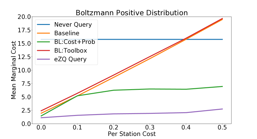
Figure 3: Per-station cost vs marginal cost of domain with Boltzmann distribution of the worker’s distances to goals.

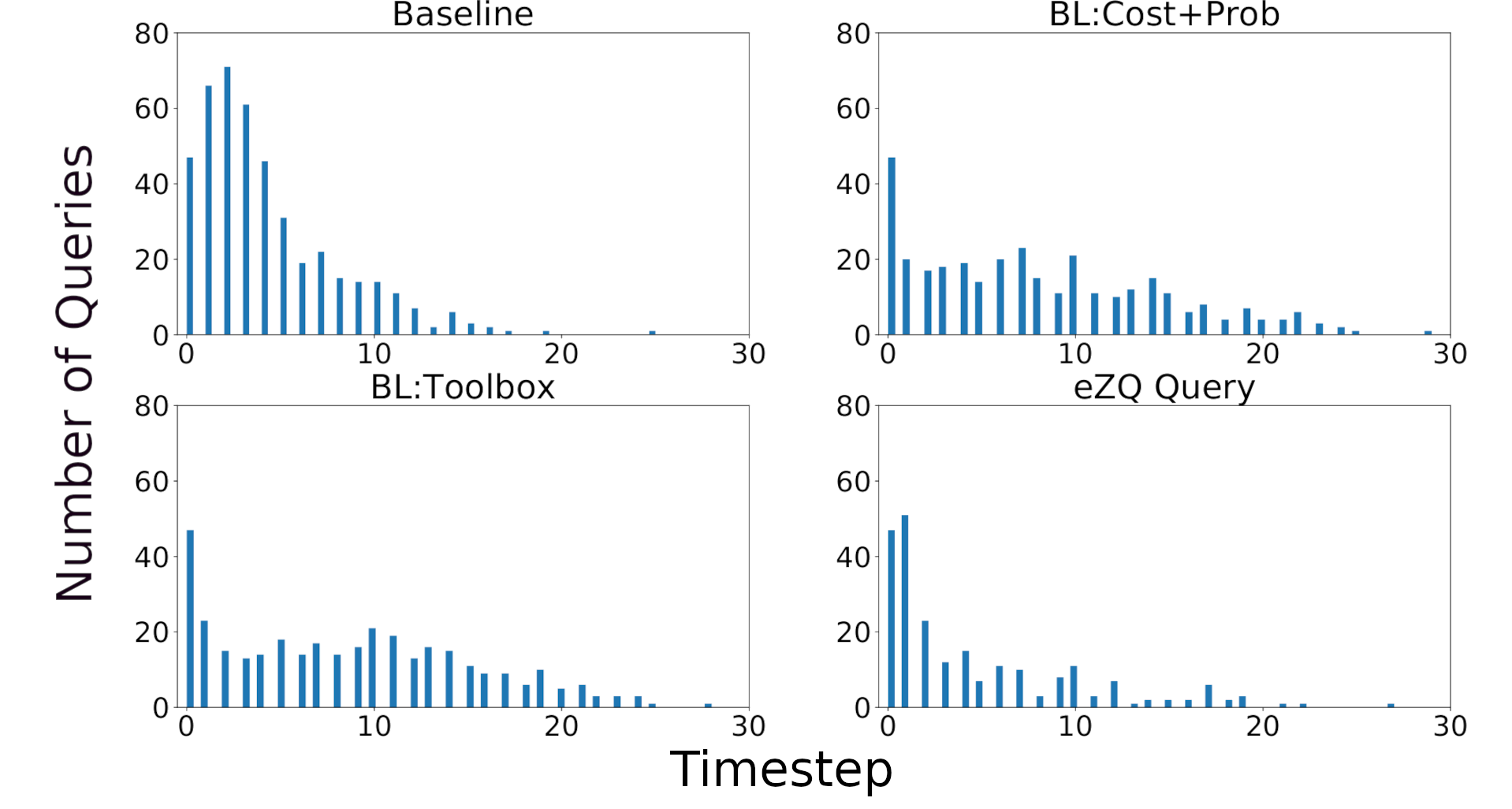
Figure 4: Histogram of number of queries (y-axis) executed per timestep (x-axis) by each method with the Boltzmann distribution of the worker’s distances to goals and a per-station cost of 0.

Figure 2 shows an example of such a tool-fetching domain. We now compare the new algorithm with previous work and the heuristics described above. We demonstrate that $eZ_{Q}$ Query is able to effectively leverage the additional information from our generalizations to obtain a better performance over previous work and the suggested heuristics, in terms of marginal cost (Definition 7).

Figure 3 shows the marginal cost averaged over 100 domain instances with different per-station costs (x-axis) when the probability distribution of the goals of the worker is the Boltzmann distribution over the worker’s distances to each goal. This distribution means that the worker is more likely to choose goals that are farther from it. $eZ_{Q}$ Query performs similarly to the heuristics when the per-station cost is 0, but dramatically outperforms all other methods as this value increases. Additional results showing $eZ_{Q}$ Query under additional goal distributions can be seen in the Appendix.

We also provide an analysis of how the $eZ_{Q}$ Query method is achieving better performance than other methods. Figure 4 shows a histogram of the number of queries executed per timestep by each method. As shown in the histogram, $eZ_{Q}$ Query tends to ask more queries in the earlier timesteps compared to BL:Toolbox and BL:Cost+Prob. This increase is because $eZ_{Q}$ Query is focused on learning the worker’s true goal with minimal cost and is better able to leverage information about the probability distribution over goals to make informed queries, and therefore finds the correct goal more quickly than other methods, but also takes longer before it knows an optimal action. In addition, we found that as the per-station cost increases from $0$ to $0.5$, the total number of queries executed by $eZ_{Q}$ query over all simulations decreases by $23\%$, showing that $eZ_{Q}$ Query executes fewer queries when the cost is higher.

Finally, there is an increased computational cost of using $eZ_{Q}$ Query over other approaches and the proposed heuristics. While calculating edp is expensive and takes several orders of magnitude longer than the rest of the querying algorithm (several hours per domain on average), these values can be computed a priori regardless of the teammate’s actions. As such, the following results are under the assumption that the edp computation is performed in advance, and the following time measurements do not include these offline computations. On average, all heuristic methods took $<0.23$ seconds to complete each simulation, while $eZ_{Q}$ Query took on average $8.9$ seconds on an Ubuntu 16.04 LTS Intel core i7 2.5 GHz, with the genetic algorithm taking on average $6.1$ seconds to run. In practice, the increased time should not be a major detriment. If a robot is communicating with either a human or another robot, the major bottleneck is likely to be the communication channel (e.g. speech, network speed, decision making of the other agent) rather than this time. In addition, when using a genetic algorithm for optimization as we do in this paper, the $eZ_{Q}$ Query computation should only grow in terms of $O(|G|^{2}log(|G|))$ with the number of goals (assuming that edp is precomputed ahead of time and that the number of members and generations do not grow with the number of goals).

Discussion and Future Work

In this paper, we investigated a new metric to quantify ambiguity of teammate policies in ad hoc teamwork settings, by estimating the expected divergence point between different policies a teammate might posses. We then utilized this metric to construct a new ad hoc agent that reasons both about when it is beneficial to query, but also about what is beneficial to query about in order to reduce the ambiguity about its teammate’s goal. Our empirical results show that regardless of the goal-choosing policy of the worker and a varying query cost model, $eZ_{Q}$ Query remains more effective than any of the other methods tested, and even when querying is almost never beneficial, it is still able to adapt and obtain performance that is consistently better than Never Query.

The scope of this work is limited to somali cat problems. In addition, our current methods are designed to work in relatively simple environments with finite state spaces and a limited number of goals. However, the edp formalization opens up new avenues for investigating other complicated somali cat scenarios and other cat scenarios, such as those in which an agent can advise or share its beliefs with its teammates. We conjecture that the $eZ_{Q}$ algorithm can be modified relatively easily to address such challenges, as long as the ego agent remains the initiator of the communication. For instance, edp may be able to be calculated in domains with larger and continuous state spaces by leveraging more sophisticated RL techniques than the policy evaluation algorithm. It might be more challenging to extend this work to domains in which the teammate is the one to initiate the communication, as other works have investigated in the context of reinforcement learning agents (Torrey and Taylor 2013; Cui and Niekum 2018). Nonetheless, this work provides the means to investigate collaborations in ad hoc settings in new contexts, while presenting concrete solutions for planning in somali cat settings.

Appendix A Algorithm Description

To calculate edp for two policies, we use a modified policy evaluation algorithm (Bellman 1966) using the Bellman update provided in Theorem 1. Algorithm 2 shows this calculation: it performs sweeps of the whole state space until all values converge within some error bound $\epsilon$. The main loop updates the estimate of edp for each state using the Bellman Equation 1 in the main paper.

Algorithm 2 Calculate EDP

procedure EDP(policy $\pi_{1}$, policy $\pi_{2}$, state space $S$, action space $A$, transition function $T$, desired accuracy $\epsilon$)

     $EDP\leftarrow\{0|s\in S\}$

     $err\leftarrow\infty$

     while $err>\epsilon$ do

         $err\leftarrow 0$

         $old\leftarrow EDP$

         for $s\in S$ do

              $A^{\prime}\leftarrow\{a\in A|\pi_{1}(s,a)>0\}$

              $EDP[s]\leftarrow[1-\sum\limits_{a\in A^{\prime}}\pi_{2}(s,a)]$

              $EDP[s]\leftarrow EDP[s]+\sum\limits_{a\in A^{\prime}}[\pi_{2}(s,a)]*\sum\limits_{s^{\prime}\in S}T(s,a,s^{\prime})*[1+old[s^{\prime}]]$

              $err\leftarrow\max{(err,|EDP[s]-old[s]|)}$

         end for

     end while

end procedure

Appendix B Experimental Setup

In this section we discuss additional details about the algorithms we tested and the experimental setup to allow reproducibility. In particular, we discuss further details about the BL:Cost+Prob querying strategy and describe in detail how instances of the Tool Fetching Domain were generated.

BL:Cost+Prob

The goal of this method is to use a heuristic to determine what the ego agent should query about after we have determined that a query could be beneficial. We first start by solving a simpler problem: determining what to query when the probability distribution over goals is uniform and every query has a uniform cost. Previous work would query about half the relevant goals, or in other words perform a binary search over the goals (Mirsky et al. 2020). However reasoning more thoroughly regarding which goals to ask about can give even better performance. Consider the pairs of goals $G_{B}=\{(g_{i},g_{j})|t\in Z_{B}(g_{i},g_{j})\}$ where $t$ is the current time and $g_{i},g_{j}\in G_{B}$ is a set of all $N$ possible goals that might still be the true goal of the worker. We can construct a binary vector $\vec{x}$ of length $N$ such that if $x_{i}$ is the $i$-th value in that vector, then station $g_{i}$ is included in the query if and only if $x_{i}=1$. A query that asks about a subset of goals $G^{\prime}\subseteq G$ will disambiguate between the sets $G^{\prime}$ and $G\setminus G^{\prime}$. Therefore, to increase the information gained from the query, we want to split the pairs of goals $(g_{i},g_{j})$ as evenly as possible between $G^{\prime}$ and $G\setminus G^{\prime}$. We can write this maximization goal as follows:

$$\max\sum\limits_{(g_{i},g_{j})\in G_{B}}(x_{i}\oplus x_{j})$$ (6)

The term in the objective is 1 only when one $x$ is 0 and the other is 1. So for instance if the next action to reach goal $g_{1}$ must be the ontic action $o_{1}$, and the next action to reach goal $g_{2}$ must be the ontic action $o_{2}\neq o_{1}$, then we need to eliminate one of these goals as a possibility before we know the next optimal ontic action. This objective ensures that the query would ask about only one of these goals, and therefore about information that is the most relevant to which ontic action the ego agent should take next.

While the above is an improvement over randomly querying, it can give undesirable behavior when there is a non-uniform probability distribution over the worker’s possible goals. To reason about such circumstances, we modify the objective to weigh the goals by the ad-hoc agent’s current belief state $P(g)$:

$$\max\sum\limits_{(g_{i},g_{j})\in G_{B}}(P(g_{i})+P(g_{j}))*(x_{i}\oplus x_{j})$$ (7)

where $P(g_{i})$ refers to the probability that the worker’s goal is $g_{i}$. Intuitively, this new equation will prioritize goals that are more likely. This is desirable, since if a goal already has an extremely low probability, it likely won’t be beneficial to query about it. We sum the two probabilities together since we want to consider these goals in the query if either of them is the true goal.

Finally, a complete model needs to incorporate different query cost models. Since we want to minimize the needed query cost as part of our objective, we add the negative cost of the query to our objective. Consequently, the final objective becomes

$$\max\sum\limits_{(g_{i},g_{j})\in G_{B}}(x_{i}\oplus x_{j})*(P(g_{i})+P(g_{j}))-\sum\limits_{i}(x_{i}*\textit{sc})$$ (8)

where sc is the cost of including a station in a query. This objective now simultaneously attempts to maximize the probability that the ego agent will be able to act in the next timestep and minimize the cost of the query. Whenever the planning algorithm decides on querying, we solve Equation 8 using the Coin-OR Integer Program solver (Forrest et al. 2018).

Domain Instance Generation

When generating a new domain instance, we first randomly select locations in the grid for the workstations and the toolboxes. Each location is chosen with uniform probability, where the only constraint is that two workstations/toolboxes cannot be in the same location. Then for each workstation, we assign its corresponding tool to one of the toolboxes with uniform probability, which means that different toolboxes might have a different number of tools in them. Finally, we choose a location for the worker and fetcher using uniform probability, and calculate the edp and wcd for each pair of stations/toolboxes as required for each of the algorithms. We serialize these results, and reuse them whenever running experiments. We generated 100 domain instances of 20x20 grids, with 50 workstations and 5 toolbox locations that were used in all experiments. Experiments were run using a custom OpenAI Gym Environment (Brockman et al. 2016).

Appendix C Additional Results

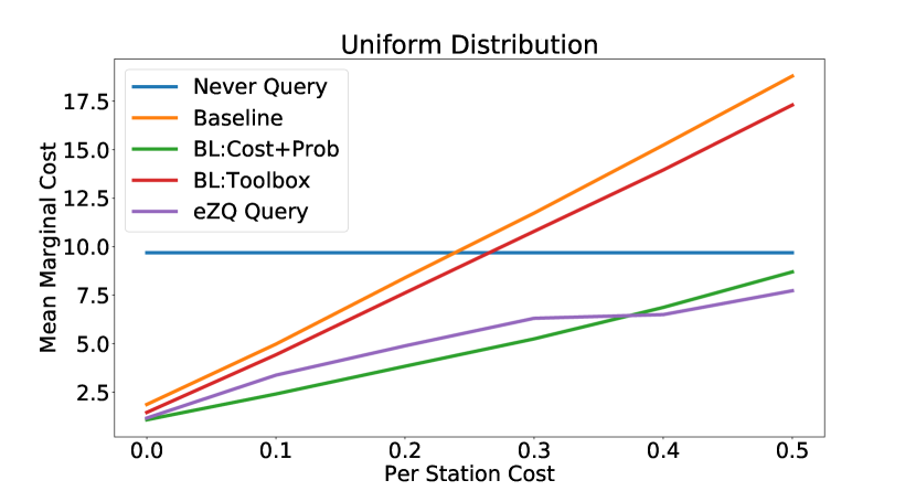
Figure 5: Per-station cost vs. marginal cost of domains with uniform distribution over the goals of the worker.

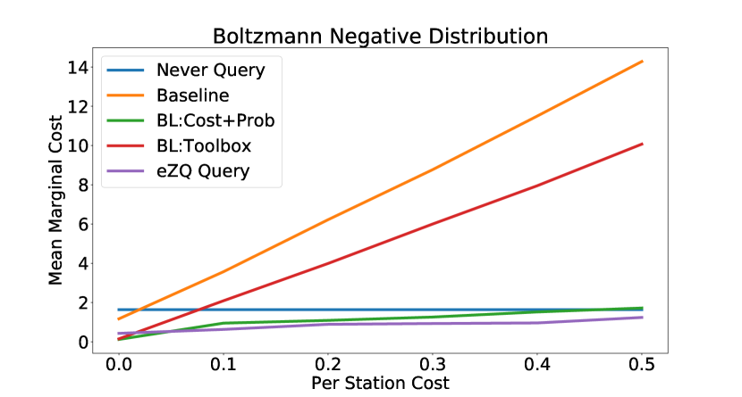
Figure 6: Per station cost vs marginal cost of domain with Boltzmann distribution of the negative of worker’s distances to goals.

In our empirical results, we showed the performance of various querying strategies with the Boltzmann distribution over the worker’s distances to goals. We present here the performance of the same strategies when using two additional distributions, a Uniform distribution and the Boltzmann distribution over the negative of the worker’s distances to goals. The Uniform distribution means that all goals are equally probable, and the Boltzmann distribution over the negative of the worker’s distances means that the worker is more likely to choose goals that are closer to it. Figure 5 shows the marginal cost with a uniform probability distribution. $eZ_{Q}$ Query exhibits equivalent performance to other approaches when the per-station cost is $0$. As the per-station cost increases, the performance of the Baseline methods dramatically worsen and none except BL:Cost+Prob outperforms Never Query when the per-station cost is large enough. By contrast, $eZ_{Q}$ Query continues to perform well and is robust to the varying query costs. Figure 6 shows the average marginal cost with the Boltzmann distribution over the negative of the worker’s distances to goals as the probability distribution. While the potential benefit from querying decreases under this distribution of potential goals, $eZ_{Q}$ Query still outperforms all other querying strategies. BL:Toolbox and BL:Cost+Prob mildly outperform $eZ_{Q}$ Query when the per-station cost is 0. However, $eZ_{Q}$ Query is the only one to consistently outperform Never Query when the per-station cost increases. Never Query in this scenario performs extremely well since when the worker chooses a goal that’s close to its current location, it reveals its true goal through its actions rather quickly. This dramatically reduces the overall need for querying in the first place. However, $eZ_{Q}$ Query is still able to adapt and obtain performance that is consistently better than Never Query.

With two exceptions, $eZ_{Q}$ Query performs significantly better than all other approaches with a p value $<0.05$. The first exception is BL:Cost+Prob with a uniform distribution over goals and a per-station cost $\leq 0.4$. The second exception is BL:Cost+Prob with a Boltzmann distribution over the negative distances to goals and per station cost $\leq 0.2$. We conjecture that our method fails to outperform BL:Cost+Prob under these conditions because there was less information for our method to leverage. For instance, when the distribution over goals is uniform and the per-station cost is 0, asking “is your goal one of stations 1, 2 or 3?” is effectively the same query as “is your goal one of stations 1, 2, 3 or 4?”. This property makes it more difficult for our genetic algorithm to optimize, and can lead to worse performance.

References

- Albrecht and Stone (2017) Albrecht, S. V.; and Stone, P. 2017. Reasoning about hypothetical agent behaviours and their parameters. In AAMAS, 547–555.
- Albrecht and Stone (2018) Albrecht, S. V.; and Stone, P. 2018. Autonomous agents modelling other agents: A comprehensive survey and open problems. Artificial Intelligence 258: 66–95.
- Barrett et al. (2014) Barrett, S.; Agmon, N.; Hazon, N.; Kraus, S.; and Stone, P. 2014. Communicating with unknown teammates. In AAMAS, 1433–1434.
- Bellman (1966) Bellman, R. 1966. Dynamic programming. Science 153(3731): 34–37.
- Brockman et al. (2016) Brockman, G.; Cheung, V.; Pettersson, L.; Schneider, J.; Schulman, J.; Tang, J.; and Zaremba, W. 2016. OpenAI Gym.
- Cakmak and Thomaz (2012) Cakmak, M.; and Thomaz, A. L. 2012. Designing robot learners that ask good questions. In ACM/IEEE international conference on Human-Robot Interaction.
- Chakraborty et al. (2017) Chakraborty, M.; Chua, K. Y. P.; Das, S.; and Juba, B. 2017. Coordinated vs. Decentralized Exploration In Multi-Agent Multi-Armed Bandits. In IJCAI, 164–170.
- Cohen, Levesque, and Smith (1997) Cohen, P. R.; Levesque, H. J.; and Smith, I. A. 1997. On team formation. Synthese Library 87–114.
- Cui and Niekum (2018) Cui, Y.; and Niekum, S. 2018. Active reward learning from critiques. In 2018 IEEE International Conference on Robotics and Automation (ICRA), 6907–6914. IEEE.
- Decker (1987) Decker, K. S. 1987. Distributed problem-solving techniques: A survey. IEEE transactions on systems, man, and cybernetics 17(5): 729–740.
- Fern et al. (2007) Fern, A.; Natarajan, S.; Judah, K.; and Tadepalli, P. 2007. A Decision-Theoretic Model of Assistance. In IJCAI, 1879–1884.
- Foerster et al. (2016) Foerster, J.; Assael, I. A.; de Freitas, N.; and Whiteson, S. 2016. Learning to communicate with deep multi-agent reinforcement learning. In NIPS, 2137–2145.
- Forrest et al. (2018) Forrest, J.; Ralphs, T.; Vigerske, S.; LouHafer; Kristjansson, B.; jpfasano; EdwinStraver; Lubin, M.; Santos, H. G.; rlougee; and Saltzman, M. 2018. coin-or/Cbc: Version 2.9.9. doi:10.5281/zenodo.1317566. URL https://doi.org/10.5281/zenodo.1317566.
- Goldman and Zilberstein (2004) Goldman, C. V.; and Zilberstein, S. 2004. Decentralized control of cooperative systems: Categorization and complexity analysis. Journal of artificial intelligence research 22: 143–174.
- Hernandez-Leal, Kartal, and Taylor (2019) Hernandez-Leal, P.; Kartal, B.; and Taylor, M. E. 2019. A survey and critique of multiagent deep reinforcement learning. AAMAS 1–48.
- Keren, Gal, and Karpas (2014) Keren, S.; Gal, A.; and Karpas, E. 2014. Goal recognition design. In ICAPS.
- Macke, Mirsky, and Stone (2020) Macke, W.; Mirsky, R.; and Stone, P. 2020. Query Content in Sequential One-shot Multi-Agent Limited Inquires when Communicating in Ad Hoc Teamwork. In Workshop on Distributed and Multi-Agent Planning (DMAP) at the International Conference on Automated Planning and Scheduling (ICAPS).
- Mirsky et al. (2020) Mirsky, R.; Macke, W.; Wang, A.; Yedidsion, H.; and Stone, P. 2020. A Penny for Your Thoughts: The Value of Communication in Ad Hoc Teamwork. International Joint Conference on Artificial Intelligence (IJCAI) .
- Mirsky et al. (2018) Mirsky, R.; Stern, R.; Gal, K.; and Kalech, M. 2018. Sequential plan recognition: An iterative approach to disambiguating between hypotheses. Artificial Intelligence 260: 51–73.
- Mordatch and Abbeel (2018) Mordatch, I.; and Abbeel, P. 2018. Emergence of grounded compositional language in multi-agent populations. In AAAI.
- Muise et al. (2015) Muise, C.; Belle, V.; Felli, P.; McIlraith, S.; Miller, T.; Pearce, A. R.; and Sonenberg, L. 2015. Planning over multi-agent epistemic states: A classical planning approach. In Twenty-Ninth AAAI Conference on Artificial Intelligence.
- Pita et al. (2008) Pita, J.; Jain, M.; Marecki, J.; Ordóñez, F.; Portway, C.; Tambe, M.; Western, C.; Paruchuri, P.; and Kraus, S. 2008. Deployed ARMOR protection: the application of a game theoretic model for security at the Los Angeles International Airport. In Proceedings of the 7th international joint conference on Autonomous agents and multiagent systems: industrial track, 125–132.
- Pynadath and Tambe (2002) Pynadath, D. V.; and Tambe, M. 2002. The communicative multiagent team decision problem: Analyzing teamwork theories and models. Journal of artificial intelligence research 16: 389–423.
- Ravula, Alkoby, and Stone (2019) Ravula, M.; Alkoby, S.; and Stone, P. 2019. Ad hoc teamwork with behavior switching agents. In IJCAI.
- Shvo and McIlraith (2020) Shvo, M.; and McIlraith, S. A. 2020. Active Goal Recognition. In AAAI.
- Stone et al. (2010) Stone, P.; Kaminka, G. A.; Kraus, S.; and Rosenschein, J. S. 2010. Ad hoc autonomous agent teams: Collaboration without pre-coordination. In AAAI.
- Stone et al. (2013) Stone, P.; Kaminka, G. A.; Kraus, S.; Rosenschein, J. S.; and Agmon, N. 2013. Teaching and leading an ad hoc teammate: Collaboration without pre-coordination. Artificial Intelligence 203: 35–65.
- Torrey and Taylor (2013) Torrey, L.; and Taylor, M. 2013. Teaching on a budget: Agents advising agents in reinforcement learning. In AAMAS, 1053–1060.
- van Zoelen et al. (2020) van Zoelen, E. M.; Cremers, A.; Dignum, F. P.; van Diggelen, J.; and Peeters, M. M. 2020. Learning to Communicate Proactively in Human-Agent Teaming. In International Conference on Practical Applications of Agents and Multi-Agent Systems, 238–249. Springer.
- Wang et al. (2020) Wang, R. E.; Wu, S. A.; Evans, J. A.; Tenenbaum, J. B.; Parkes, D. C.; and Kleiman-Weiner, M. 2020. Too many cooks: Coordinating multi-agent collaboration through inverse planning. AAMAS .
- Wayllace, Hou, and Yeoh (2017) Wayllace, C.; Hou, P.; and Yeoh, W. 2017. New Metrics and Algorithms for Stochastic Goal Recognition Design Problems. In IJCAI, 4455–4462.