Information-geometry of physics-informed statistical manifolds and its use in data assimilation

Abstract

The data-aware method of distributions (DA-MD) is a low-dimension data assimilation procedure to forecast the behavior of dynamical systems described by differential equations. It combines sequential Bayesian update with the MD, such that the former utilizes available observations while the latter propagates the (joint) probability distribution of the uncertain system state(s). The core of DA-MD is the minimization of a distance between an observation and a prediction in distributional terms, with prior and posterior distributions constrained on a statistical manifold defined by the MD. We leverage the information-geometric properties of the statistical manifold to reduce predictive uncertainty via data assimilation. Specifically, we exploit the information geometric structures induced by two discrepancy metrics, the Kullback-Leibler divergence and the Wasserstein distance, which explicitly yield natural gradient descent. To further accelerate optimization, we build a deep neural network as a surrogate model for the MD that enables automatic differentiation. The manifold’s geometry is quantified without sampling, yielding an accurate approximation of the gradient descent direction. Our numerical experiments demonstrate that accounting for the information-geometry of the manifold significantly reduces the computational cost of data assimilation by facilitating the calculation of gradients and by reducing the number of required iterations. Both storage needs and computational cost depend on the dimensionality of a statistical manifold, which is typically small by MD construction. When convergence is achieved, the Kullback-Leibler and $L_{2}$ Wasserstein metrics have similar performances, with the former being more sensitive to poor choices of the prior.

Keywords Method of Distributions  $\cdot$ Data assimilation  $\cdot$ Uncertainty Reduction  $\cdot$ Machine Learning

1 Introduction

Mathematical models used to represent “reality” are invariably faulty due to a number of mutually reinforcing reasons such as lack of detailed knowledge of the relevant laws of nature, scarcity (in quality and/or quantity) of observations, and inherent spatiotemporal variability of the coefficients used in their parameterizations. Consequently, model predictions must be accompanied by a quantifiable measure of predictive uncertainty (e.g., error bars or confidence intervals); when available, observations should be used to reduce this uncertainty. The probabilistic framework provides a natural means to achieve both goals. For example, a random forcing in Langevin (stochastic ordinary-differential) equations [1] or fluctuating Navier-Stokes (stochastic partial-differential) equations [2] implicitly account for sub-scale variability and processes that are otherwise absent in the underlying model.

Solutions of such stochastic models, and of models with random coefficients, are given in terms of the (joint) probability density function (PDF) or cumulative distribution function (CDF) of the system state(s). They can be computed, with various degrees of accuracy and ranges of applicability, by employing, e.g., Monte Carlo simulations (MCS), polynomial chaos expansions (PCE) and the method of distributions (MD) [3]. MCS are robust, straightforward and trivially parallelizable; yet, they carry (often prohibitively) high computational cost. PCE rely on a finite-dimensional expansion of the solution of a stochastic model; their accuracy and computational efficiency decrease as the correlation length of the random inputs decreases (the so-called curse of dimensionality), making them ill-suited to problems with white noise. The MD yields a (generally approximate) partial differential equation (PDE) for the PDF or CDF of a system state (henceforth referred to as a PDF/CDF equation). The MD can handle inputs with both long and short correlations, although the correlation length might affect the robustness of the underlying closure approximations when the latter are needed. For Langevin systems driven by white noise, the MD yields a Fokker-Planck equation [1] for a system state’s PDF. For colored (correlated) noise, PDF/CDF equations become approximate [4], although their computational footprint typically does not change. If a Langevin system is characterized by $N_{\text{st}}$ system states, then PDF/CDF equations are defined in an augmented $N_{\text{st}}$-dimensional space. Their MD-based derivation requires a closure approximation [3, and references therein] such as the semi-local closure [5, 6] used in our analysis because of its accuracy and manageable computational cost.

The temporal evolution of the PDF of a system state predicted with, e.g., the MD provides a measure of the model’s predictive uncertainty in the absence of observations of the system state. In the lingo of Bayesian statistics, this PDF serves as a prior that can be improved (converted into the posterior PDF) via Bayesian update as data become available. When used in combination with ensemble methods like MCS, standard strategies for Bayesian data assimilation, e.g., Markov chain Monte Carlo (MCMC) and its variants, are often prohibitively expensive [7]. The computational expedience is the primary reason for the widespread use of various flavors of Kalman filter, which perform well when the system state’s PDF is (nearly) Gaussian and models are linear, but are known to fail otherwise. Data-aware MD (DA-MD) [8] alleviates this computational bottleneck, rendering Bayesian update feasible even on a laptop. DA-MD employs the MD to propagate the system state PDF (forecast step) and sequential Bayesian update at measurement locations to assimilate data (analysis step). It offers two major benefits. First, the MD replaces repeated model runs, characteristic of both MCMC [9] and ensemble and particle filters [10, 11], with the solution of a single deterministic equation for the evolving PDF. Second, it dramatically reduces the dimensionality of the PDFs involved in the Bayesian update at each assimilation step because it relies on a single-point PDF rather than a multi-point PDF whose dimensionality is determined by the discretized state being updated. DA-MD takes advantage of the MD’s ability to handle nonlinear models and non-Gaussian distributions [12, 13].

DA-MD recasts data assimilation as a minimization problem, whose loss function represents the discrepancy between observed and predicted posterior distributions. The observed posterior PDF is obtained by direct application of Bayes’ rule at the measurement point, combining the data model and a prior PDF computed via the MD. The predicted PDF is assumed to obey the PDF equation, which acts as a PDE constraint for the loss function. The parameters appearing in the MD are the target of minimization and introduce a suitable parameterization for the space of probabilities (a statistical manifold) with quantifiable geometric properties. The computational effort of DA-MD is thus determined by the efficiency in the solution of a minimization problem on a manifold. This aspect of DA-MD is the central focus of our analysis, in which we exploit information-geometric theory to reformulate the optimization problem by relying on the geometric properties of the MD-defined manifold.

We utilize results from the optimal transport theory and machine learning. Specifically, we employ both the Kullback-Leibler (KL) divergence and the $L_{2}$ Wasserstein distance to measure the discrepancy between predicted and observed posterior distributions at each assimilation point. The former underpins much of information theory [14] and variational inference [15], while the latter has its origins in optimal transport and is now increasingly popular in the wider machine learning community [16]. We employ gradient descent (GD) and natural gradient descent (NGD) for optimization [17], with preconditioning matrices expressing the geometry induced on the statistical manifold by the choice of the discrepancy. These formulations are explicit for univariate distributions; thus, they ideally suit our data assimilation procedure.

Finally, we construct a surrogate model for the solution of the PDF/CDF equation to accelerate sequential minimization of loss functions, taking advantage of the relatively small dimensionality of the statistical manifold. We identify a special architecture of a deep neural network (DNN) that enables the calculation of the terms involved in NGD for both discrepancy choices. The use of DNNs obviates the need to resort to sampling when assessing the manifold’s geometry, a strategy that has a debatable success [18].

The paper is organized as follows. In section 2, we briefly overview the tools and concepts from information geometry and optimal transport that are directly relevant to the subsequent analysis. In section 3, we summarize the DA-MD approach (with details in appendix A) and illustrate how the information-geometric tools and the MD can be naturally combined to reduce predictive uncertainty. Section 4 contains results of our numerical experiments conducted on a Langevin equation with either white or colored noise. Main conclusions drawn from this study are summarized in section 5.

2 Preliminaries

Let ${}_{p}\mathcal{P}(\mathbb{R}^{d})$ denote the probability space of PDFs $f$ on $\mathbb{R}^{d}$ with finite $p$th moments, where $p\geq 1$. Our key objective is to minimize loss functions involving PDFs $f$ belonging to ${}_{p}\mathcal{P}(\mathbb{R}^{d})$. In this section, we summarize definitions, tools and theoretical results that will be subsequently used in concert with DA-MD.

Measures of discrepancy.

Alongside classic measures of discrepancy between generic integrable functions $f_{1}(\mathbf{X}),f_{2}(\mathbf{X}):\mathbb{R}^{d}\rightarrow\mathbb{R}^{+}$ such as the $L_{1}$ and the $L_{2}$ norms,

$$d_{1}(f_{1},f_{2}):=\int_{\mathbb{R}^{d}}|f_{1}(\mathbf{X})-f_{2}(\mathbf{X})|\text{d}\mathbf{X}\quad\text{and}\quad d_{2}(f_{1},f_{2}):=\left(\int_{\mathbb{R}^{2}}|f_{1}(\mathbf{X})-f_{2}(\mathbf{X})|^{2}\text{d}\mathbf{X}\right)^{1/2},$$

we utilize measures of discrepancy that are tailored to the underlying geometry of the probabilistic space ${}_{p}\mathcal{P}(\mathbb{R}^{d})$. The KL divergence,

$$d_{\text{KL}}(f_{1},f_{2}):=\int_{\mathbb{R}^{d}}f_{1}(\mathbf{X})\ln\frac{f_{1}(\mathbf{X})}{f_{2}(\mathbf{X})}\text{d}\mathbf{X},$$ (1)

expresses the discrepancy between the PDFs $f_{1}$ and $f_{2}$ in terms of relative entropy. Used to quantify how well $f_{1}:\mathbb{R}^{d}\rightarrow{}_{p}\mathcal{P}(\mathbb{R}^{d})$ approximates $f_{2}:\mathbb{R}^{d}\rightarrow{}_{p}\mathcal{P}(\mathbb{R}^{d})$, the KL divergence is not a distance since $d_{\text{KL}}(f_{1},f_{2})\neq d_{\text{KL}}(f_{2},f_{1})$.

Another discrepancy measure is the $p$-Wasserstein distance,

$$W_{p}(f_{1},f_{2}):=\left(\underset{\gamma\in\Gamma(f_{1},f_{2})}{\inf}\int_{\mathbb{R}^{d}\times\mathbb{R}^{d}}\|\mathbf{X}-\mathbf{Y}\|^{p}\gamma(\text{d}\mathbf{X},\text{d}\mathbf{Y})\right)^{1/p},\quad p\geq 1,$$ (2)

where $\Gamma$ is the set of joint probability measures $\gamma$ on $\mathbb{R}^{d}\times\mathbb{R}^{d}$ whose marginals are univariate probability measures corresponding to $f_{1}$ and $f_{2}$. Originating in the field of optimal transport, (2) quantifies the optimal (infimum) cost of shifting the mass distribution of $f_{1}$ to $f_{2}$. Such minimum exists and is unique under regularity conditions for the univariate PDFs for $p>1$, i.e., $f$ must be absolutely continuous with respect to the Lebesgue measure [19]. For $d=1$, (2) reduces to [20]

$$W_{p}(f_{1},f_{2})=\|F_{1}^{-1}(Y)-F_{2}^{-1}(Y)\|_{p}=\left(\int_{0}^{1}|F_{1}^{-1}(Y)-F_{2}^{-1}(Y)|^{p}\text{d}Y\right)^{1/p},\quad p\geq 1,$$ (3)

where $F_{i}(X)=\int_{-\infty}^{X}f_{i}(X)\text{d}X$ with $i=1,2$ is the CDF corresponding to the PDF $f_{i}(X)$; and $F_{i}^{-1}(Y)$ is the inverse of $F_{i}$ defined as $F_{i}^{-1}(Y)=\inf\{X:F_{i}(X)\geq Y,Y\in(0,1)\}$.

Since DA-MD deals with univariate distributions, we are concerned with $d=1$.

Approximation of distributions.

Various fields of science and engineering—e.g., machine learning [21, 22], estimation theory [23], and optimal transport and control theory [19, 24, 25]—deal with a problem of approximating an (empirical) target PDF $\hat{f}(X)$ with a PDF $f(X;\boldsymbol{\varphi}):\mathbb{R}\rightarrow\mathcal{P}_{\boldsymbol{\varphi}}(\mathbb{R})$ defined on the parameterized probability space $\mathcal{P}_{\boldsymbol{\varphi}}$. The latter consists of PDFs that are uniquely characterized by a set of $N_{\text{par}}$ parameters $\boldsymbol{\varphi}\in\Phi\subset\mathbb{R}^{N_{\text{par}}}$ with $N_{\text{par}}\geq 1$. This functional approximation is recast as a problem of finding a parameter set that minimizes a function $\mathcal{C}(\boldsymbol{\varphi})$ depending on a selected measure of discrepancy $D(\boldsymbol{\varphi})$ between the target PDF $\hat{f}(X)$ and its approximation $f(X;\boldsymbol{\varphi})$,

$$\underset{\boldsymbol{\varphi}\in\Phi}{\text{argmin}}\;\mathcal{C}(D(\boldsymbol{\varphi})),\quad\text{with}\;D(\boldsymbol{\varphi})=D(f(X;\boldsymbol{\varphi}),\hat{f}(X)),$$ (4)

with $f(X;\boldsymbol{\varphi})$ belonging to $\mathcal{P}_{\boldsymbol{\varphi}}$. We assume $\mathcal{P}_{\boldsymbol{\varphi}}$ to be a subset of ${}_{2}{\mathcal{P}}(\mathbb{R})$. The use of the KL and $W_{2}$ metrics in place of $D$ in (4) introduces known geometries to the statistical manifold of parameterized PDFs, facilitating the deployment of predictable optimization algorithms that exploit this geometric structure. Specifically, one of the geometric properties of the KL divergence is its parameterization invariance, i.e., the equivalency between computation of the discrepancy $\mathcal{C}(\boldsymbol{\varphi})\equiv D(\boldsymbol{\varphi})\equiv d_{\text{KL}}(f(X;\boldsymbol{\varphi}),\hat{f}(X))$ in the PDF space $\mathcal{P}_{\varphi}$ and in the parameter space $\Phi$; this property facilitates minimization of the loss function via natural gradient descent [26, Sec. 2.1.3]. Moreover, a solution of the minimization problem (4) with $\mathcal{C}(\boldsymbol{\varphi})\equiv d_{\text{KL}}(f(X;\boldsymbol{\varphi}),\hat{f}(X))$ corresponds to the maximum likelihood estimate of the parameters $\boldsymbol{\varphi}$ [27]. This analogy elucidates the connection between Bayesian inference and information geometry. When $\hat{f}$ is obtained empirically (e.g., from sampling or repeated experiments), the use of the Wasserstein distance, $\mathcal{C}(\boldsymbol{\varphi})\equiv D^{2}(\boldsymbol{\varphi})/2\equiv W_{2}^{2}(f(X;\boldsymbol{\varphi}),\hat{f}(X))/2$, is more computationally expedient [19, 21, 22, 24], while possessing geometric properties almost as rigorous as KL [17].

Statistical manifolds.

Let the PDF $f(X;\boldsymbol{\varphi})$ be smooth and have a support $\Omega:=\{X\in\mathbb{R}|f(X)>0\}$. We assume this support to be compact, $\Omega=\left[X_{\text{min}},X_{\text{max}}\right]\subset\mathbb{R}$, and the dimensionality of the parameter space $\Phi\subset\mathbb{R}^{N_{\text{par}}}$ to be finite, $N_{\text{par}}<+\infty$. An $N_{\text{par}}$-dimensional manifold is an $N_{\text{par}}$-dimensional topological space that behaves locally like the Euclidean space $\mathbb{R}^{N_{\text{par}}}$. A smooth manifold is equipped with a metric tensor $\mathbf{G}(\boldsymbol{\varphi})$—which facilitates the calculation of distances on the local approximation of the manifold, i.e., the tangent plane—and an affine connection $\nabla_{\boldsymbol{\varphi}}$—which enables differentiation. The second-order tensor $\mathbf{G}$ is positive definite and varies smoothly with $\boldsymbol{\varphi}$. A statistical manifold $\mathcal{M}$ is a manifold with coordinates $\boldsymbol{\varphi}=(\varphi^{1},\dots,\varphi^{N_{\text{par}}})\in\mathbb{R}^{N_{\text{par}}}$ where each point represents a PDF with assigned support and defined features. A divergence on the statistical manifold $\mathcal{M}$ is a non-negative function $D(f(X;\boldsymbol{\varphi}),f(X;\boldsymbol{\varphi}^{\prime})):\mathcal{M}\times\mathcal{M}\rightarrow\mathbb{R}^{+}$, which is equal to zero if and only if $f(X;\boldsymbol{\varphi})\equiv f(X;\boldsymbol{\varphi}^{\prime})$ and which can be approximated locally (i.e., when $\boldsymbol{\varphi}$ and $\boldsymbol{\varphi}^{\prime}$ are close) via the components $G_{ij}$ of the second-order tensor $\mathbf{G}$ as $D(f(\boldsymbol{\varphi}),f(\boldsymbol{\varphi}^{\prime}))=G_{ij}(\boldsymbol{\varphi})\Delta\varphi^{i}\Delta\varphi^{j}/2+\mathcal{O}(|\Delta\boldsymbol{\varphi}|^{3}),$ where $\Delta\boldsymbol{\varphi}=\boldsymbol{\varphi}-\boldsymbol{\varphi}^{\prime}$ and the Einstein summation is implied over the repeated indices $i,j=1,\dots,N_{\text{par}}$. The tensor $\mathbf{G}$ defines a Riemannian metric on the statistical manifold $\mathcal{M}$, and $\mathcal{M}$ is said to be Riemannian.

Information geometry of statistical manifolds.

If the KL divergence is used to quantify the discrepancy between two PDFs on the manifold $\mathcal{M}$, then the tensor metric $\mathbf{G}(\boldsymbol{\varphi})$ (a geometric structure) of the space $\mathcal{P}_{\boldsymbol{\varphi}}$ of parameterized univariate PDFs $f(X;\boldsymbol{\varphi})$ is called Fisher information matrix,

$$\mathbf{G}_{F}(\boldsymbol{\varphi})=\int_{\Omega}\frac{1}{f(X;\boldsymbol{\varphi})}\left(\nabla_{\boldsymbol{\varphi}}f(X;\boldsymbol{\varphi})\right)^{\top}\nabla_{\boldsymbol{\varphi}}f(X;\boldsymbol{\varphi})\text{d}X.$$ (5)

The resulting statistical manifold $\mathcal{M}$ is invariant, i.e., for $\boldsymbol{\varphi}_{i}\in\Phi$ and $f_{i}\equiv f(\boldsymbol{\varphi}_{i})$ with $i=1,2$, the divergence $d_{\text{KL}}(f_{1},f_{2})$ on the manifold $\mathcal{M}$ equals the distance $|\boldsymbol{\varphi}_{1}-\boldsymbol{\varphi}_{2}|$ in the parameter space $\Phi$. This property underpins the Riemannian natural gradient descent (NGD) method (a.k.a. Fisher-Rao gradient descent) for parameter identification [28, and references therein]. The method uses the metric tensor $\mathbf{G}_{F}$ as a pre-conditioner for gradient descent algorithms to solve (4) with $\mathcal{C}\equiv D\equiv d_{\text{KL}}$,

$$\boldsymbol{\varphi}_{k+1}=\boldsymbol{\varphi}_{k}-\eta\mathbf{G}_{F}^{-1}(\boldsymbol{\varphi}_{k})\nabla_{\boldsymbol{\varphi}}d_{\text{KL}}(f(X;\boldsymbol{\varphi}),\hat{f})|_{\boldsymbol{\varphi}_{k}},$$ (6)

where $\eta$ is the descent step and $\mathbf{G}_{F}^{-1}$ is the inverse of $\mathbf{G}_{F}$. The technique presents strong theoretical analogies with classic filtering techniques (namely Kalman filter and extended Kalman filter) [29, 30]. In the absence of an analytical expression for $\mathbf{G}_{F}$, the matrix can be approximated empirically, although with debatable accuracy [18].

Geometric structure, including the metric tensor $\mathbf{G}_{W}(\boldsymbol{\varphi})$, of the finite-dimensional Wasserstein manifolds of Gaussian PDFs was studied in [31, 32]. These results were subsequently generalized to construct $\mathbf{G}_{W}(\boldsymbol{\varphi})$ for the manifolds $\mathcal{M}$ of generic discrete [28] and continuous [17] distributions. Specifically, when $d=1$, the Wasserstein manifold’s metric tensor $\mathbf{G}_{W}$ has an explicit form,

$$\mathbf{G}_{W}(\boldsymbol{\varphi})=\int\frac{1}{f(X;\boldsymbol{\varphi})}\left(\nabla_{\boldsymbol{\varphi}}F(X;\boldsymbol{\varphi})\right)^{\top}\nabla_{\boldsymbol{\varphi}}F(X;\boldsymbol{\varphi})\text{d}X.$$ (7)

Under some mild regularity assumptions, the finite-dimensional Wasserstein manifold $\mathcal{M}$ in the parameter space $\Phi$ is Riemannian [17]. It introduces an NGD in the space $\Phi$,

$$\boldsymbol{\varphi}_{k+1}=\boldsymbol{\varphi}_{k}-\eta\mathbf{G}_{W}^{-1}(\boldsymbol{\varphi}_{k})\nabla_{\boldsymbol{\varphi}}\mathcal{C}(\boldsymbol{\varphi})|_{\boldsymbol{\varphi}_{k}},\quad\text{with}\quad\mathcal{C}\equiv\frac{1}{2}D^{2}\;\text{and}\;D\equiv W_{2}.$$ (8)

Remark 2.1

Regardless of whether one chooses the KL divergence or the $W_{2}$ distance, NGD orients the optimization problem (8) according to the topology of the statistical manifold $\mathcal{M}$ as expressed by its metric tensor $\mathbf{G}_{i}$ ($i=F$ or $W$), thus accelerating the solution. The computational cost of both (6) and (8) depends on the overall number of iterations and on the calculation of $\mathbf{G}_{i}$ (storage cost $\mathcal{O}(N_{\text{par}}^{2})$ per iteration) and its inverse $\mathbf{G}_{i}^{-1}$ (inversion cost $\mathcal{O}(N_{\text{par}}^{3})$ per iteration) [26]. Thus, the overall cost of optimization is a trade-off between the number of iterations, arguably reduced on information-geometric grounds, and the cost of inverting the metric tensor $\mathbf{G}_{i}$.

Remark 2.2

The finite-dimensional $L_{2}$-Wasserstein manifold $\mathcal{M}$ is not exactly geodesic (unless PDFs are Gaussian), and as such the geodesic distance on the manifold is not identical to $W_{2}$ [17]. As demonstrated by [17, Th. 1 and Prop. 6], the natural gradient trajectory approximates the geodesic distance up to second order information.

Remark 2.3

A unifying framework connecting the KL and $W_{2}$ metrics for manifolds of discrete distributions is proposed in [33, 34].

3 DA-MD with DNN Surrogates

Consider a state variable $x(t):\mathbb{R}^{+}\rightarrow\mathbb{R}$, whose dynamics is governed by a stochastic/random ordinary differential equation

$$\frac{\text{d}x(t)}{\text{d}t}=s(x(t);w(t),\boldsymbol{\theta}),\qquad t>0;$$ (9a)

subject to a (possibly uncertain, i.e., random) initial condition

$$x(t=0)=x_{0},\qquad x_{0}\in\mathbb{R}.$$ (9b)

The system is driven by the stationary (statistically homogeneous) random process $w(t)$ characterized by a single-point PDF $f_{w}(W;t)$ and a two-point auto-correlation function $\rho_{w}(|t_{1}-t_{2}|)$; these functions involve meta-parameters ${\boldsymbol{\varphi}}_{w}$ such as the mean, variance, and correlation length of $w(t)$. The deterministic function $s(x;\cdot)$, parameterized by a set of $N_{\theta}$ (possibly uncertain, i.e., random) coefficients ${\boldsymbol{\theta}}\in\mathbb{R}^{N_{\theta}}$, is such that a solution to (9) is smooth almost surely in the probability space of both $w(t)$ and, possibly, $\boldsymbol{\theta}$ and $x_{0}$. If $\boldsymbol{\theta}$ and $x_{0}$ are random, then they are characterized by PDFs $f_{\boldsymbol{\theta}}(\boldsymbol{\Theta})$ and $f_{0}(X)$, with meta-parameters ${\boldsymbol{\varphi}}_{\theta}$ and ${\boldsymbol{\varphi}}_{0}$, respectively. In all, the statistics of $x(t)$ depends on the set of $N_{\text{par}}$ meta-parameters $\boldsymbol{\varphi}=(\boldsymbol{\varphi}_{w},\boldsymbol{\varphi}_{\theta},\boldsymbol{\varphi}_{0})\in\Phi\subset\mathbb{R}^{N_{\text{par}}}$.

In addition to being described by the model (9), the system state $x(t)$ is sampled at $N_{\text{meas}}$ times $t_{1},\dots,t_{N_{\text{meas}}}$. The noisy observations $\hat{\mathbf{x}}=\{\hat{x}_{1},\dots,\hat{x}_{N_{\text{meas}}}\}$ satisfy the data model

$$\hat{x}_{m}=x(t_{m})+\varepsilon_{m},\qquad m=1,\dots,N_{\text{meas}},$$ (10)

where the Gaussian measurement errors $\varepsilon_{m}$ are mutually uncorrelated and have zero mean and variance $\sigma_{\varepsilon}^{2}$.

A goal of data assimilation (DA) is to improve model predictions by augmenting them with observations. Some DA methods yield the “best” (i.e., unbiased) prediction and quantify its predictive uncertainty in terms of, respectively, the ensemble mean, $\langle x(t)\rangle$, and the standard deviation, $\sigma_{x}(t)$, of the state variable $x(t)$. These statistics provide but limited information about $x(t)$, unless its single-point PDF $f(X;t)$ is Gaussian or a known map thereof. Bayesian update and particle filters are examples of DA strategies that overcome this limitation by seeking a solution of (9) in terms of the PDF $f(X;t)$—or the corresponding CDF $F(X;t)=\mathbb{P}[x(t)\leq X]$—updated with the data $\hat{\mathbf{x}}$ in (10). Computing such distributions with ensemble methods requires a large number of repeated solves of (9), which can be prohibitively expensive.

Data assimilation via DA-MD [8] aims to significantly accelerate the computation. Like many other DA strategies, DA-MD comprises two steps: forecast and analysis. The first of these steps relies on the model (9) and makes a prediction of the system state at time $t$ in terms of $f(X;t)$ or $F(X;t)$. Rather than using, e.g., Monte Carlo simulations, the MD [3] implements this step by deriving a deterministic equation for $f(X;t)$ or $F(X;t)$. Thus, the single-point CDF $F(X;t)$ of the state variable $x(t)$ in (9) satisfies (sometime approximately) a parabolic PDE (appendix A)

$$\frac{\partial F}{\partial t}+\mathcal{U}(X,t;\boldsymbol{\varphi})\frac{\partial F}{\partial X}=\frac{\partial}{\partial X}\left(\mathcal{D}(X,t;\boldsymbol{\varphi})\frac{\partial F}{\partial X}\right),\qquad t>0,\quad X\in\Omega=[X_{\text{min}},X_{\text{max}}],$$ (11a)

subject to initial and boundary conditions

$$F(X;0)=F_{0}(X),\qquad F(X_{\text{min}},t)=0,\qquad F(X_{\text{max}},t)=1.$$ (11b)

The drift velocity, $\mathcal{U}(X,t;\boldsymbol{\varphi}):\Omega\times\mathbb{R}^{+}\rightarrow\mathbb{R}$, and the diffusion coefficient, $\mathcal{D}(X;t,\boldsymbol{\varphi}):\Omega\times\mathbb{R}^{+}\rightarrow\mathbb{R}^{+}$, are smooth functions of their arguments, which involve a set of the meta-parameters $\boldsymbol{\varphi}$. The functional forms $\mathcal{U}$ and $\mathcal{D}$ depend on that of $s(x;\cdot)$, on the statistical characterization of the random parameters epitomized by the statistical parameters ${\boldsymbol{\varphi}}$ of their distributions, and on the degree of approximation introduced by the closure strategy. If the initial state of the system, $x_{0}$, is known with certainty, then its CDF $F_{0}(X)$ is the Heaviside step function, $F_{0}(X)=\mathcal{H}(X-x_{0})$.

Remark 3.1

The CDF equation (11) maps the meta-parameters ${\boldsymbol{\varphi}}$ onto $F(X;t,\boldsymbol{\varphi})$, the CDF of the system state $x(t)$. In other words, a point $\boldsymbol{\varphi}\in\Phi\subset\mathbb{R}^{N_{\text{par}}}$ can be thought of as a coordinate on the statistical manifold $\mathcal{M}$ of the CDF $F(X;t,\boldsymbol{\varphi})$ at time $t$. At any time $t^{\prime}$, a solution to (11) provides an estimate of the CDF $F(X;t^{\prime},\boldsymbol{\varphi})$ dependent on the current characterization of the random inputs expressed by $\boldsymbol{\varphi}$. Equivalently, points $\widetilde{\boldsymbol{\varphi}}=\{t,{\boldsymbol{\varphi}}\}$ define a dynamic statistical manifold $\mathcal{M}_{t}$ of the CDF $F(X;\widetilde{\boldsymbol{\varphi}})$.

The second step of DA-MD, analysis via Bayesian update, is performed sequentially for each of the $N_{\text{meas}}$ measurements $\hat{x}_{m}$ in (10). At $m$th assimilation step, the updated meta-parameters $\boldsymbol{\varphi}^{(m)}$ are computed by solving the minimization problem (4) for the discrepancy $D$ between the CDF $F(X;t_{m},\boldsymbol{\varphi})$ predicted by the model (11) and the observational CDF obtained with Bayes’ rule,

$$\hat{F}(X;t_{m})=\int_{X_{\text{min}}}^{X}\hat{f}(X;t_{m})\text{d}X\quad\text{with}\quad\hat{f}(X;t_{m})=\frac{f_{L}(\hat{x}_{m}|x(t_{m})=X)f(X;t_{m},\boldsymbol{\varphi}^{(m-1)})}{\int_{\Omega}f_{L}(\hat{x}_{m}|x(t_{m})=X)f(X;t_{m},\boldsymbol{\varphi}^{(m-1)})\text{d}X}.$$ (12)

Here the likelihood function $f_{L}(\hat{x}_{m}|x(t_{m})=X)$ specifies a data model; and the PDF $f(X;t_{m},\boldsymbol{\varphi}^{(m-1)})$, computed by solving the CDF equation (11) with the parameter set $\boldsymbol{\varphi}^{(m-1)}$ from the previous assimilation step, serves as a prior. In [8], the discrepancy $D$ was expressed in terms of the $L_{2}$ norm; a consequence of this choice was significant computational cost of solving the minimization problem (4). A main innovation of this study is to exploit the geometric structure of the statistical manifolds in the parameter space $\Phi$ by using either the KL divergence (1) or the Wasserstein distance (3) at each assimilation time. This enables us to solve (4) via NGD, which we henceforth refer to as NGD-KL and NGD-W₂ depending on which metric is used. The update of the meta-parameters $\boldsymbol{\varphi}$ is done using NGD-KL (6) or NGD-W₂ (8), taking advantage of the explicit formulations for the manifold’s metric tensors $\mathbf{G}_{F}$ in (5) and $\mathbf{G}_{W}$ in (7).

Remark 3.2

The analysis step of DA-MD is performed on univariate (one-point) distributions ($d=1$) regardless of the size of the physical parameter and meta-parameter sets, $N_{\theta}$ and $N_{\text{par}}$. That drastically reduces (to one) the dimensionality of the update effort in classical Bayesian DA. Moreover, availability of a CDF/PDF equation removes the need for Gaussianity and linearity assumptions on the physical model and its random parameters. The CDF/PDF equation is assumed to be valid throughout the assimilation process.

Remark 3.3

Parameter update via discrepancy minimization places DA-MD in the company of many machine-learning and optimal-transport techniques (see the references above). Unlike these methods, DA-MD uses CDF or PDF equations and their parameters to define the parameter space for a statistical manifold $\boldsymbol{\varphi}$, such that the discrepancy minimization is constrained by these PDEs. Learning occurs on the statistical manifold defined by $\boldsymbol{\varphi}$ and proceeds by sequential updates of these meta-parameters.

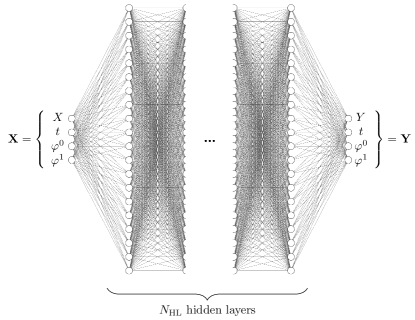
Figure 1: Fully-connected DNN used to approximate a solution of the CDF equation (11), with $N_{\text{HL}}$ hidden layers and $N_{\text{nphl}}$ nodes per hidden layer. Inputs are $\mathbf{X}\{X=F^{-1}(Y;t,\boldsymbol{\varphi}),t,\boldsymbol{\varphi},\}$, and outputs are $\mathbf{Y}=\{Y=F(X;t,\boldsymbol{\varphi}),t,\boldsymbol{\varphi}\}$. This illustration has $N_{\text{par}}=2$, with $\boldsymbol{\varphi}=\{\varphi^{0},\varphi^{1}\}$. The DNN parameters, in both the illustration and our numerical examples, are set to $N_{\text{HL}}=7$, $N_{\text{nphl}}=20$.

Loss function minimization.

We use a surrogate model to accelerate the calculation of the discrepancies $d_{\text{KL}}(f(X;\boldsymbol{\varphi}),\hat{f})$ or $W_{2}(f(X;\boldsymbol{\varphi}),\hat{f})$, their respective gradients $\nabla_{\boldsymbol{\varphi}}d_{\text{KL}}$ or $\nabla_{\boldsymbol{\varphi}}W_{2}$, and the preconditioning tensor metrics $\mathbf{G}_{F}$ or $\mathbf{G}_{W}$. Specifically, a fully-connected deep neural network (DNN), whose architecture is illustrated in fig. 1, is used to approximate the solution of the CDF equation given the set of inputs $\mathbf{X}=\{X,t,\boldsymbol{\varphi}\}$. The number of outputs in this DNN equals the number of inputs, $\mathbf{Y}=\{Y_{j}:j=1,\dots,N_{\text{par}}+2\}=\{Y=F(X;t,\boldsymbol{\varphi}),t,\boldsymbol{\varphi}\}$, such that $\text{dim}({\mathbf{X}})=\text{dim}(\mathbf{Y})=N_{\text{par}}+2$. We require the resulting vector function $\mathbf{Y}=\mathbf{F}(\mathbf{X})$ to be one-to-one except at singularity points, and its derivative to be an invertible linear map in local, identifiable regions. These requirements fulfill the hypotheses of the Inverse Function Theorems [37, Th. 1-2 in sec. 3.2] for vector functions. Under these conditions, the vector function $\mathbf{Y}=\mathbf{F}(\mathbf{X})$ is invertible, its inverse is differentiable, and the derivative of the inverse is equal to the inverse of the derivative [37, Th. 3 in sec. 3.2]. Automatic differentiation is employed both to verify the inversion theorem hypotheses and to calculate the terms appearing in the minimization algorithms. This is especially useful, since NGD-KL utilizes the derivatives of the forward pass, whereas NGD-W₂ requires the derivatives of the inverse function. A differentiable DNN allows accurate calculation of the metric tensors for both geometries, eliminating potential problems related to their empirical approximation.

The DNN is trained on a data set consisting of $N_{\text{ts}}$ pairs $(\mathbf{X}_{\text{ts}}^{i},\mathbf{Y}_{\text{ts}}^{i})$, for $i=1,\dots,N_{\text{ts}}$. This training set is generated by solving the CDF equation (11) for $N_{\text{ts}}$ combinations of meta-parameters $\boldsymbol{\varphi}$, i.e., at points $\boldsymbol{\varphi}_{i}\in\Phi$ with $i=1,\dots,N_{\text{ts}}$. The DNN training is accomplished by solving an optimization problem [38],

$$\underset{\mathbf{w},\mathbf{b}}{\text{argmin}}(\text{MSE}_{\text{ts}}+\text{MSE}_{\text{R}}+\text{MSE}_{\text{aux}}+\text{SMR}),$$ (13a)

with respect to the weights and biases of the DNN, $$\mathbf{w} \mathbf{b}$$ and , respectively. Here,

$$\text{MSE}_{\text{ts}}=\sum_{j=1}^{n+2}\lambda_{j}\frac{1}{N_{\text{ts}}}\sum_{i=1}^{N_{\text{ts}}}|Y_{j}(\mathbf{X}_{\text{ts}}^{i})-Y_{j,\text{ts}}^{i}|^{2},\quad\lambda_{j}=\left(\max Y_{j,\text{ts}}\right)^{-1}$$ (13b)

$$\text{MSE}_{\text{R}}=\frac{1}{N_{\text{R}}}\sum_{i=1}^{N_{\text{R}}}|R(\mathbf{X}_{\text{R}}^{i})|^{2}$$ (13c)

$$\text{MSE}_{\text{aux}}=\frac{1}{N_{\text{aux}}}\sum_{i=1}^{N_{\text{aux}}}|Y(\mathbf{X}_{\text{aux}}^{i})-Y_{\text{aux}}^{i}|^{2}$$ (13d)

$$\text{SMR}=\left(\max\left|\frac{\partial Y}{\partial X}(\mathbf{X}_{\text{SMR}})\right|\right)^{-1}\sum_{i=1}^{N_{\text{SMR}}}\max\left(0,-\frac{\partial Y}{\partial X}(\mathbf{X}_{\text{SMR}}^{i})\right),$$ (13e)

and $\mathbf{Y}(\mathbf{X}^{i})$ represents the $N_{\text{par}}+2$ outputs of the DNN with inputs $\mathbf{X}^{i}$. The mean square errors $\text{MSE}_{\text{R}}$ and $\text{MSE}_{\text{aux}}$ enforce the fulfillment of the CDF equation and its initial/boundary conditions at collocation points $\{\mathbf{X}_{\text{R}}^{i}\}_{i=1}^{N_{\text{R}}}$ and $\{\mathbf{X}_{\text{aux}}^{i}\}_{i=1}^{N_{\text{aux}}}$, respectively. The residual is defined as

$$R(\mathbf{X}_{\text{R}}^{i})=\frac{\partial Y(\mathbf{X}_{\text{R}}^{i})}{\partial t}+\left(\mathcal{U}(\mathbf{X}_{\text{R}}^{i})-\frac{\partial\mathcal{D}}{\partial X}(\mathbf{X}_{\text{R}}^{i})\right)\frac{\partial Y}{\partial X}(\mathbf{X}_{\text{R}}^{i})-\mathcal{D}(\mathbf{X}_{\text{R}}^{i})\frac{\partial^{2}Y}{\partial X^{2}}(\mathbf{X}_{\text{R}}^{i}),$$ (14)

and $Y_{\text{aux}}^{i}$ represent the auxiliary conditions for the CDF equation at points $\mathbf{X}_{\text{aux}}^{i}$, which represents initial or boundary conditions (11b). The term SMR is a soft constraint [39] that regularizes the DNN by enforcing monotonicity of the output $Y=F(X;t,\boldsymbol{\varphi})$ along the $X$ direction at points $\{\mathbf{X}_{\text{SMR}}^{i}\}_{i=1}^{N_{\text{SMR}}}=\{\{\mathbf{X}_{\text{ts}}^{i}\}_{i=1}^{N_{\text{R}}},\{\mathbf{X}_{\text{R}}^{i}\}_{i=1}^{N_{\text{R}}},\{\mathbf{X}_{\text{aux}}^{i}\}_{i=1}^{N_{\text{aux}}}\}$. The physics-aware component of (13), $\text{MSE}_{\text{R}}+\text{MSE}_{\text{aux}}$, makes training less data-intensive and increases confidence in the predictions of the DNN outside the training range (but within the residual points range).

4 Numerical Experiments

In this section, we apply the information-theoretic DA strategy introduced above to three problems described by (9). Section 4.1 contains an example of deterministic nonlinear dynamics starting from a random initial condition; this setting provides an ideal testbed for the information-geometric analysis by virtue of lending itself to analytical treatment. Section 4.2 deals with a Langevin equation with white noise $w(t)$, a problem for which the CDF equation (11) is exact. In other words, the forecast component of DA-MD is exact, whereas the analysis step introduces an approximation. In section 4.3, we consider a Langevin equation with colored noise $w(t)$ that is modeled as an Ornstein-Uhlenbeck process; the derivation of the CDF equation (11) requires a closure approximation. In this case, the performance of DA-MD depends also on the accuracy and robustness of the CDF equation as forecasting tool.

In all cases, one realization ($x_{0}^{\star}$ or $\boldsymbol{\theta}^{\star}$) of the relevant random parameters, $x_{0}$ or $\boldsymbol{\theta}$, represents ground truth. Statistical models for these parameters are chosen such that the state variable $x(t)$ has a compact support $\Omega\subset\mathbb{R}^{+}$. This ensures that the information geometry induced by the $W_{2}$ divergence is rigorously defined. The $N_{\text{meas}}$ observations $\hat{\mathbf{x}}$ are taken at regular time intervals, with the time step $\Delta t=t_{N_{\text{meas}}}/(N_{\text{meas}}+1)$. They are generated by adding zero-mean Gaussian noise with standard deviation $\sigma_{\varepsilon}$ to the solution of (9) with $x_{0}^{\star}$ or $\boldsymbol{\theta}^{\star}$ (i.e., the synthetic truth). This procedure results in the Gaussian likelihood function $f_{L}$, although other choices are possible. While not investigated here, data models constructed on repeated observations of the same phenomenon might be more suitable for processes that are inherently random like those described by Langevin equations.

For the Langevin scenarios in sections 4.2 and 4.3, we employ the JITCSDE Python module [40] to solve the stochastic ordinary differential equation (9). The corresponding CDF equations (11) are solved with a finite volumes (FV) scheme, implemented using the Fipy library [41], to provide a training set for the surrogate model. DNN is trained by employing Tensorflow; optimization in (13) is performed using L-BFGS-B method [42], with a random initialization of $\mathbf{w}$ and $\mathbf{b}$; and the network topology is shown in fig. 1. Automatic differentiation is used to compute both the derivatives in the residual $R$ in (14) and the PDF from CDF. Minimization of the KL and $W_{2}$ discrepancies is performed using both standard gradient descent (GD) and NGD. In the case of NGD, convergence is accelerated by the use of the pre-conditioners $\mathbf{G}_{F}$ and $\mathbf{G}_{W}$ in (6) and (8). For each direction established by the gradient of the loss function (adjusted by the pre-conditioners when NGD is used) we employ the Scipy library’s implementation of step calculation [43, Sec. 5.2]. A convergence criterion for NGD in (6) and (8) is defined by $|\nabla_{\varphi}D|\leq\epsilon$. Because of the different order of magnitude of the KL and $W_{2}$ discrepancies $D$, the convergence threshold $\epsilon$ is discrepancy-specific; we select a KL-based minimization threshold, $\epsilon_{\text{KL}}$, and assign the threshold for W₂, $\epsilon_{\text{W}_{2}}$, such that $\epsilon_{\text{W}_{2}}/\mathcal{C}(\text{W}_{2}(f(X;t_{1},\boldsymbol{\varphi}^{(0)});\hat{f}(X;t_{1})))=\epsilon_{\text{KL}}/\mathcal{C}(d_{\text{KL}}(f(X;t_{1},\boldsymbol{\varphi}^{(0)});\hat{f}(X;t_{1})))$.

4.1 Deterministic dynamics with random initial state

The dynamics of state variable $x(t)$ is described by

$$\frac{\text{d}x}{\text{d}t}=-2x^{2},\qquad x(0)=x_{0},$$ (15)

The random initial state $x_{0}$ has compact support $\Omega_{0}\subset\mathbb{R}^{+}$, which ensures that $x(t)$ has a compact support $\Omega\subset\mathbb{R}^{+}$. To be specific, and without loss of generality, we take the CDF of $x_{0}$, $F_{0}(X;\boldsymbol{\varphi}_{0})$, to be Gaussian, with assigned prior mean ($\mu_{0}^{(0)}$) and standard deviation ($\sigma_{0}^{(0)}$) acting as the sole meta-parameters for the model, i.e., $\boldsymbol{\varphi}_{0}^{(0)}=\{\mu_{0}^{(0)},\sigma_{0}^{(0)}\}=\boldsymbol{\varphi}^{(0)}$.

For this problem, the general CDF equation (11) is exact, reduces to (section A.1)

$$\frac{\partial F}{\partial t}-2X^{2}\frac{\partial F}{\partial X}=0,\qquad F(X;t=0)=F_{0}(X);$$ (16)

and has an analytical solution $F(X;t,\boldsymbol{\varphi})$ and the corresponding analytical expression for the PDF $f(X;t,\boldsymbol{\varphi})=\text{d}F/\text{d}X$. As a consequence, there is no need for a surrogate model of the solution to this CDF equation. The data assimilation problem has a computable Bayesian solution

$$f_{0}(X_{0}|\hat{\mathbf{x}})=\frac{f_{L}(\hat{\mathbf{x}}|x(t_{1:N_{\text{meas}}},X_{0}))f_{0}(X_{0})}{\int_{\Omega}f_{L}(\hat{\mathbf{x}}|x(t_{1:N_{\text{meas}}},X_{0}))\hat{f}_{0}(X_{0})\text{d}X_{0}}=\frac{\prod_{m=1}^{N_{\text{meas}}}f_{L}(\hat{x}_{m}|x(t_{m},X_{0}))f_{0}(X_{0})}{\int\prod_{m=1}^{N_{\text{meas}}}f_{L}(\hat{x}_{m}|x(t_{m},X_{0}))f_{0}(X_{0})\text{d}X_{0}},$$ (17)

where the prior PDF $f_{0}(X)$ is computed as $f_{0}=\text{d}F_{0}/\text{d}X$, and the i.i.d. measurements $\hat{x}_{m}$ are assigned the likelihood function

$$f_{L}(\hat{\mathbf{x}}|x(t_{1:N_{\text{meas}}},X_{0}))=\prod_{m=1}^{N_{\text{meas}}}f_{L}(x_{m}|x(t_{m},X_{0})).$$

We use the exact Bayesian posterior (17) to gauge the accuracy of the sequential Bayesian update of the meta-parameters $\boldsymbol{\varphi}=\boldsymbol{\varphi}_{0}$ via GD for (4) with $\mathcal{C}\equiv d_{\text{KL}}$ or $W_{2}^{2}/2$, NGD-KL (6), and NGD-W₂ (8). Assigned meta-parameters $\boldsymbol{\varphi}_{0}$ uniquely identify a distribution for the state $x(t)$ through the (analytical) solution to the CDF equation (16). A forecast PDF at the measurement time $t_{m}$, and the corresponding observational PDF $f(X;t_{m})$ is obtained via Bayes’rule

$$\hat{f}(X;t_{m}|x_{m})=\frac{f_{L}(\hat{x}_{m}|x(t_{m})=X)f(X;t_{m},\boldsymbol{\varphi}^{(m-1)})}{\int_{\Omega}f_{L}(\hat{x}_{m}|x(t_{m})=X)f(X;t_{m},\boldsymbol{\varphi}^{(m-1)})\text{d}X},$$ (18)

in which the priors $f(X;t_{m},\boldsymbol{\varphi}^{(m-1)}$ are computed analytically. The availability of analytical expressions for $F(X;t)$ and $f(X;t)$ facilitates the (semi-)analytical computation of both the metric tensors $\mathbf{G}_{F}$ and $\mathbf{G}_{W}$ in (5) and (7), and the the gradient of the discrepancy, $\nabla_{\varphi}\mathcal{D}$, for the KL an $W_{2}$ measures. The integrals in the metric tensors, the discrepancy gradient, and the normalization constant in (18), are computed via numerical quadrature from the Fortran library QUADPACK.

Figure 2 exhibits prior and posterior PDFs of the random initial state $x_{0}$, obtained alternatively with the four DA-MD implementations—GD for (4) with $D\equiv d_{\text{KL}}$ or $W_{2}$, NGD-KL (6), and NGD-W₂ (8)—and with the analytical Bayesian update (17). The information-geometric optimization strategies NGD-KL and NGD-W₂ have comparable performance, both reproducing accurately the exact Bayesian posterior and having negligible difference in the identified meta-parameters $\boldsymbol{\varphi}$ at the end of the assimilation window. After assimilation of $N_{\text{meas}}=10$ measurements, the unknown ground truth $x_{0}^{\star}=0.954$ is approximated by the mean of the posterior PDF, $\mu_{0}^{(N_{\text{meas}})}\equiv\varphi_{1}^{(N_{\text{meas}})}$; the standard deviation of this PDF, $\sigma_{0}^{(N_{\text{meas}})}\equiv\varphi_{2}^{(N_{\text{meas}})}$, provides a measure of predictive uncertainty. These statistics are $\boldsymbol{\varphi}^{(N_{\text{meas}})}=\{0.88,0.09\}$ for all optimization algorithms.

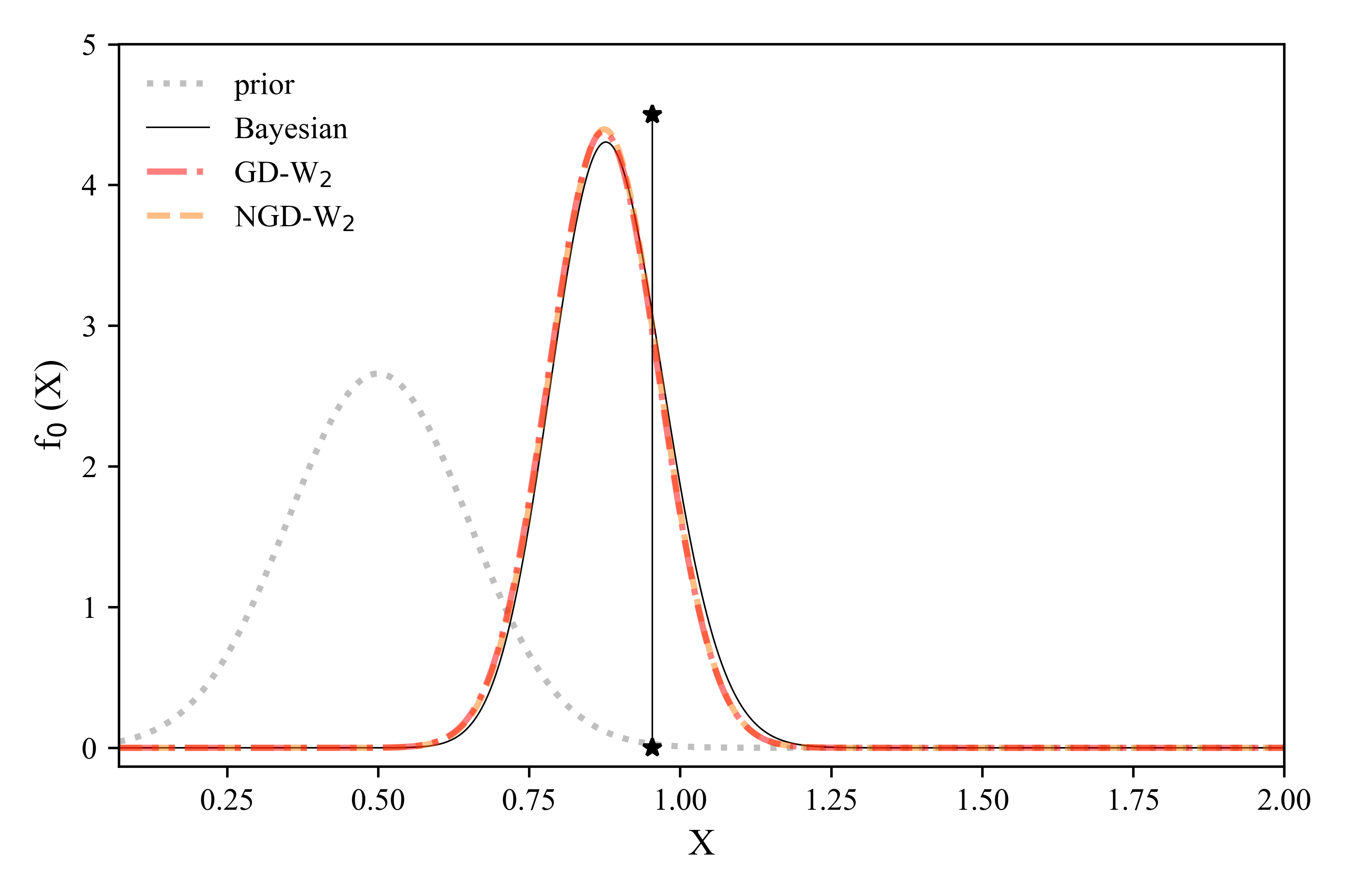
Figure 2: Prior and posterior PDFs of the initial state $x_{0}$ after assimilation of $N_{\text{meas}}=10$ observations, computed with the information-geometric optimization strategies NGD-KL (left) and NGD-W₂ (right). Also plotted are the analytically derived Bayesian posterior (solid line) and the posteriors obtained with GD-KL (dash-dotted line on the left) and GD-W₂ (dash-dotted line on the left). The ground truth, $x_{0}^{\star}=0.954$, is indicated by the starred vertical line. Simulation parameters are set to $\sigma_{\varepsilon}=0.1$, $t_{N_{\text{meas}}}=2$, $\boldsymbol{\varphi}^{(0)}=(0.5,0.15)$, $\epsilon_{\text{KL}}=10^{-3}$.

Figure 3 shows the number of iterations, $N_{\text{iter}}$, it takes each of the four DA methods to converge at each assimilation step of DA-MD. If the KL divergence is used as a discrepancy metric, NGD converges in consistently fewer iterations than GD does; if the $W_{2}$ distance is used instead, then NGD and GD require on average the same number of iterations to converge. That is possibly because the $W_{2}$-induced loss function $\mathcal{C}(\boldsymbol{\varphi})\equiv W_{2}(f(X;\boldsymbol{\varphi}),\hat{f}(X))^{2}/2$ is smoother than its KL-induced counterpart (as shown in fig. 4 for $m=1$) and, hence, the availability of the analytical gradient $\nabla_{\boldsymbol{\varphi}}D$ is as helpful as the preconditioning. NGD is expected to become more beneficial when the loss functions is more sensitive to some parameters than to others, or when parameters vary in widely different ranges.

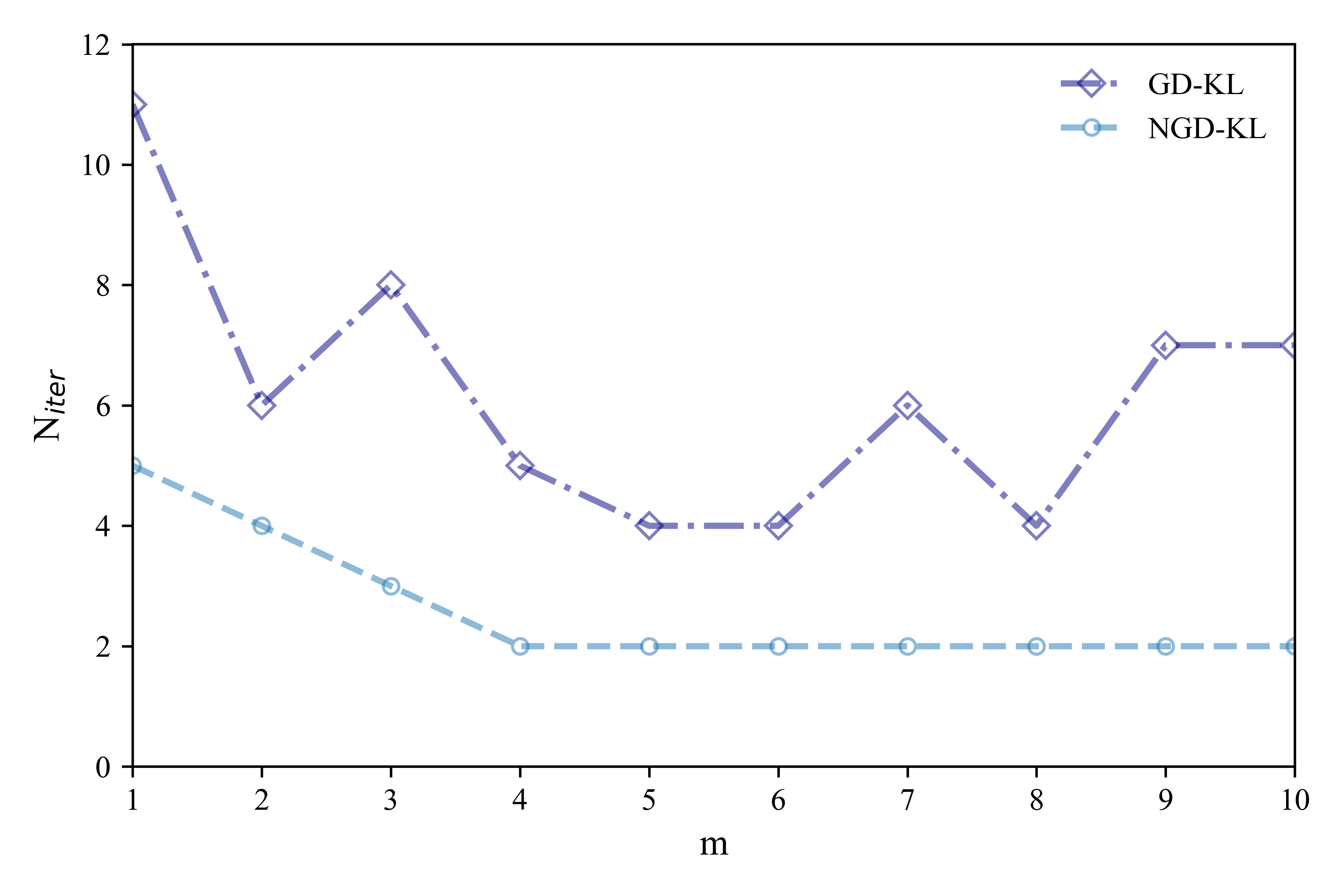
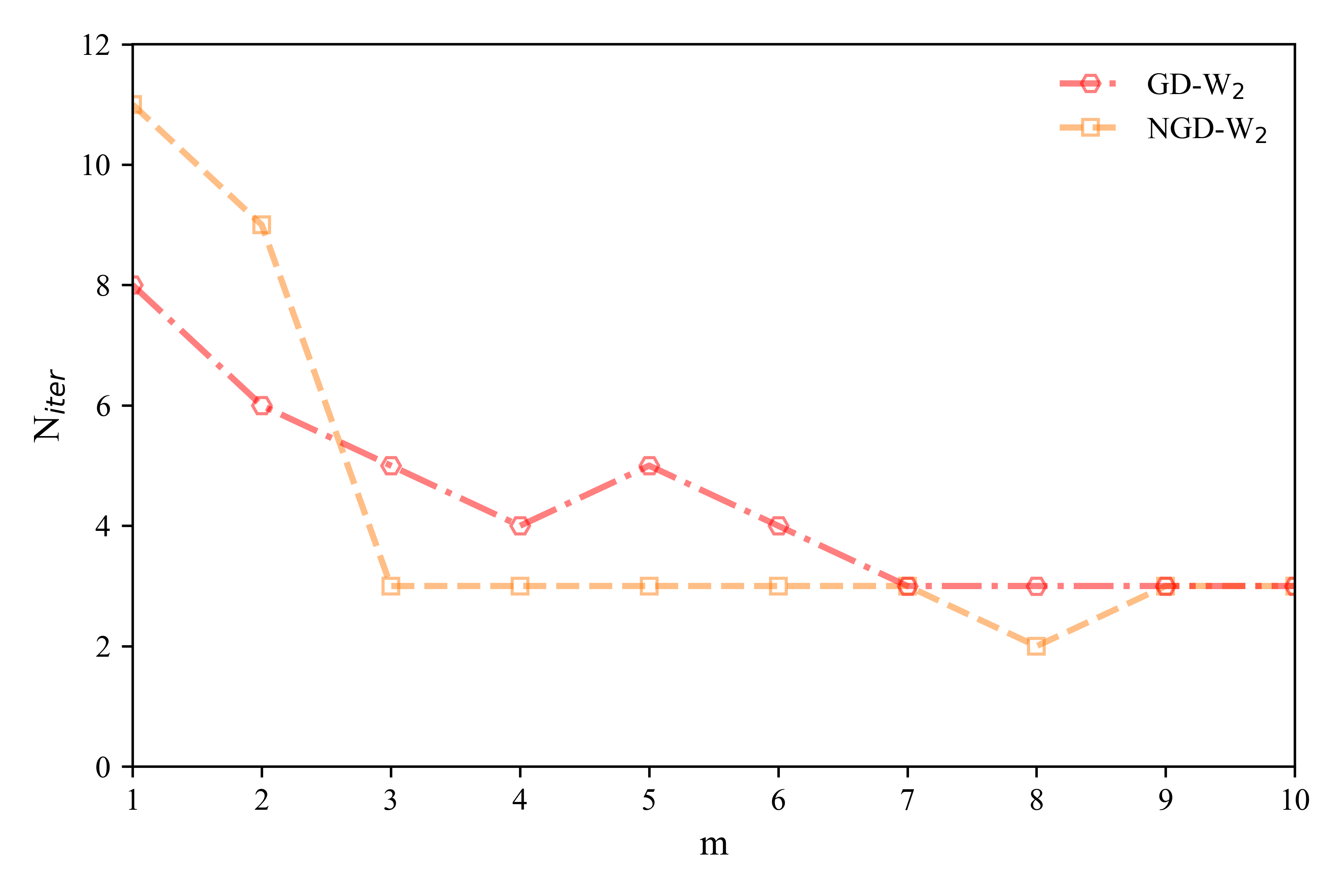
Figure 3: Number of iterations to solve the minimization problem (4) at the $m$th assimilation step with GD (dash-dotted line) and NGD (dashed line) when the KL (left) and $W_{2}$ (right) discrepancies are used. The simulation parameter values are the same as in fig. 2.

The total computational cost depends not only on the number of iterations, but also on the time required to compute the necessary terms at each iteration. Each NGD iteration is more expensive than GD’s because it requires the calculation of a preconditioning matrix (i.e., the metric tensors for the geometry of the manifold), with a number of operations $\mathcal{O}(N_{\text{par}}^{3})$ (see remark 2.1). When the evaluation of either the loss function or its gradient is computationally expensive, the computational time for GD would significantly increase.

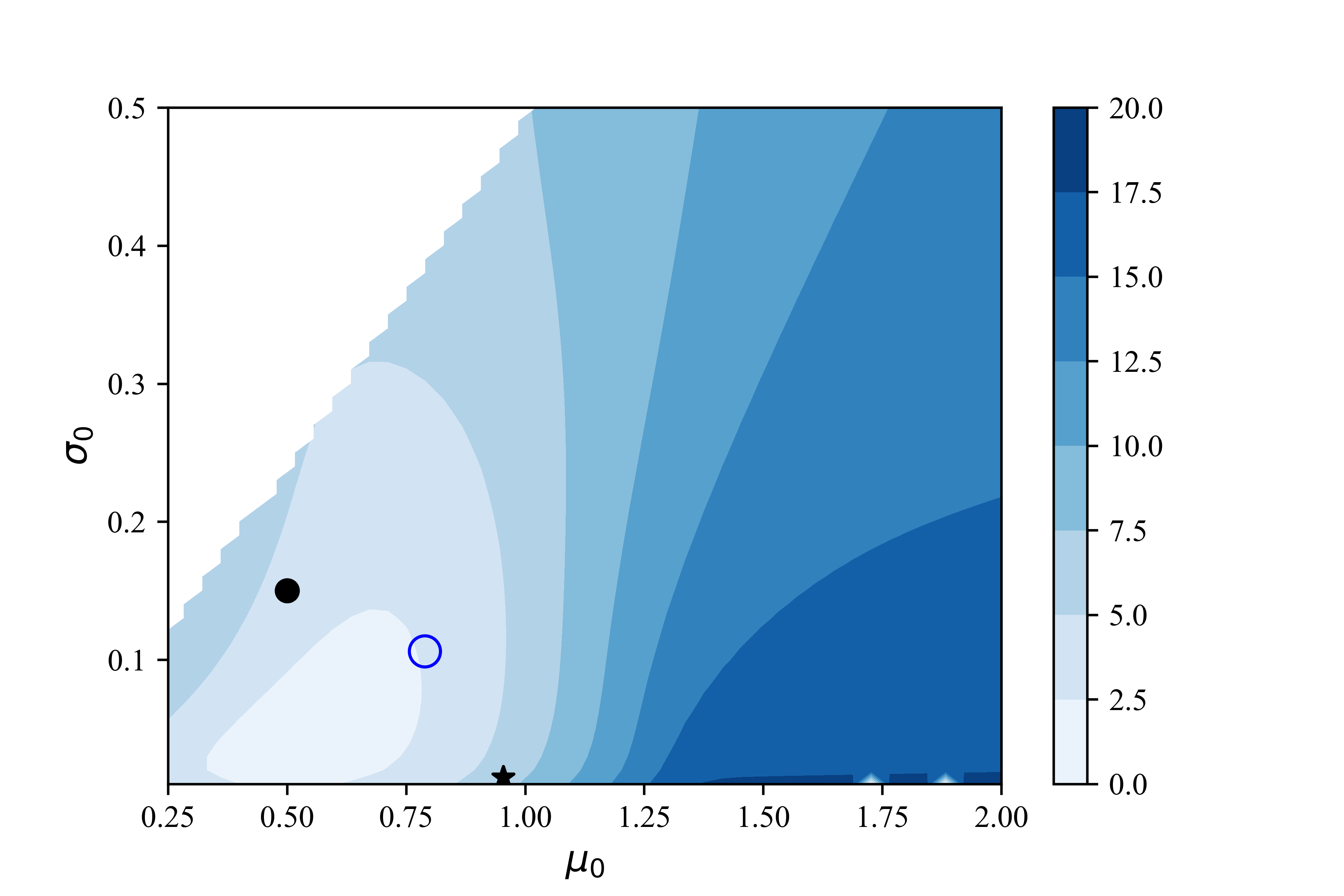
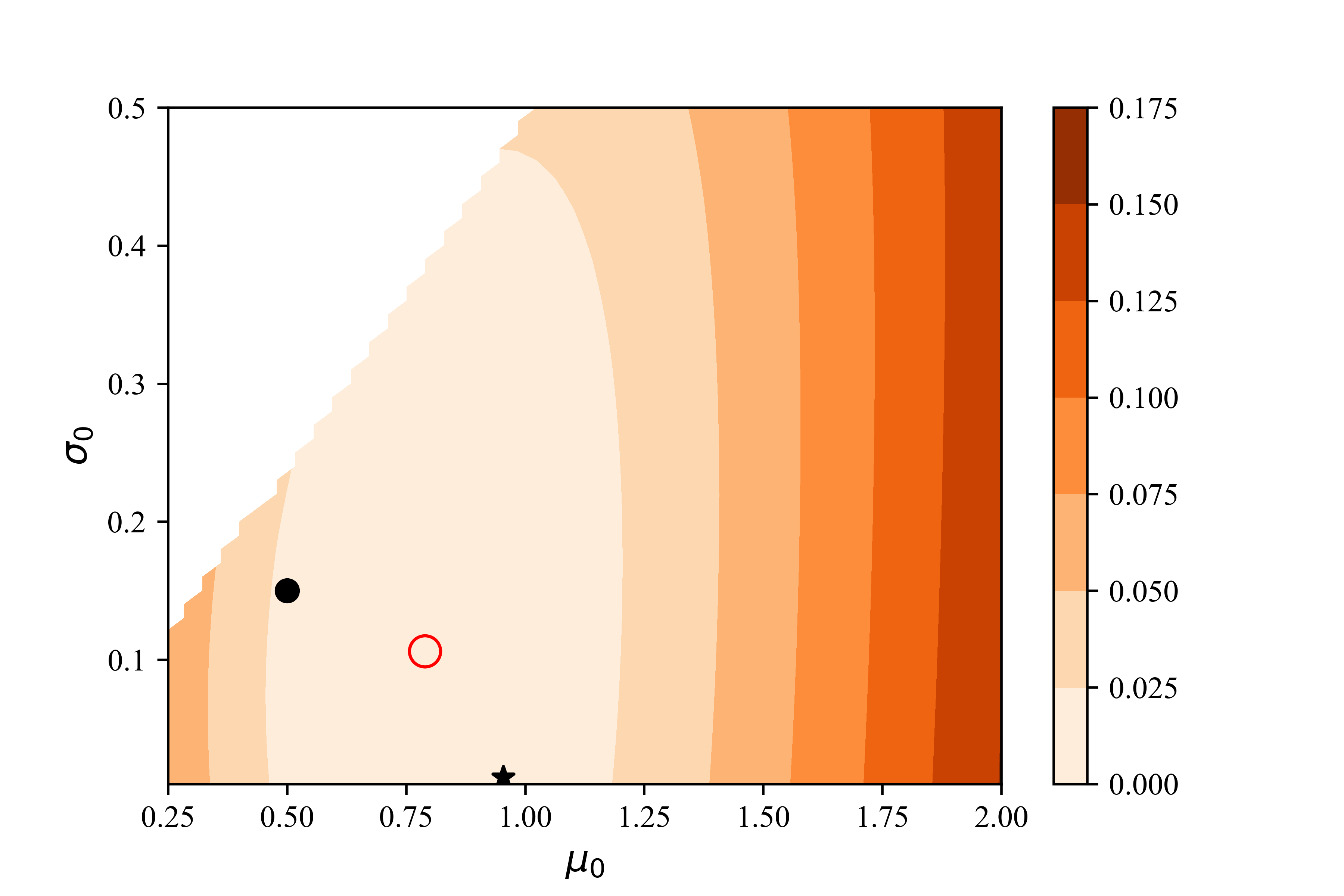
Figure 4: Loss functions for KL (left) and W₂ divergence (right) for the random initial condition test case in the parameter space $\boldsymbol{\varphi}=\boldsymbol{\varphi}_{0}=\{\mu_{0},\sigma_{0}\}$ at $m=1$ (assimilation of the first measurement). The small (full) circle in both panels indicates the prior parameters $\boldsymbol{\varphi}^{(0)}$, the star indicates the true value $\{x_{0}^{\star},0\}$. The large (empty) circle represents the first update of the parameters, $\boldsymbol{\varphi}^{(1)}$, obtained via NGD optimization. The blank region is to guarantee that $x_{0}$ is positive almost surely. The simulation parameter values are the same as in fig. 2.

As a final note, we found the calculation of the KL loss to be more sensitive to the initial guess, with poor choices of the prior often resulting in poor convergence of the DA-MD procedure. That is caused by the high sensitivity of the KL divergence to the shape of the distributions, especially when they are very far apart and/or very sharp, resulting in poor numerical accuracy of the integration (1).

4.2 Langevin equation with white noise

The dynamics of state variable $x(t)$ is described by a Langevin equation,

$$\frac{\text{d}x}{\text{d}t}=-a(t)x(t),\qquad x(0)=x_{0}^{\star},$$ (19)

where the statistically homogeneous (stationary) random process $a(t)=\mu_{a}+\sigma_{a}w(t)$ has mean $\mu_{a}$ and standard deviation $\sigma_{a}$, with $w(t)$ denoting standard Gaussian white noise. The initial state $x_{0}^{\star}\in\mathbb{R}^{+}$ is deterministic. The process $a(t)$ is almost surely positive, which ensures that $x(t)$ has a compact support $\Omega\subset\mathbb{R}^{+}$ and, hence, the information geometry induced by the $W_{2}$ distance is rigorously defined.

The single-point CDF $F(X;t)$ of the state variable $x(t)$ in (19) satisfies exactly a CDF equation (appendix A)

$$\frac{\partial F}{\partial t}-\mu_{a}X\frac{\partial F}{\partial X}=\frac{1}{2}\frac{\partial}{\partial X}\left(\sigma_{a}^{2}X^{2}\frac{\partial F}{\partial X}\right),$$ (20a)

subject to initial and boundary conditions

$$F(x;0)=\mathcal{H}(X-x_{0}^{\star}),\qquad F(X_{\text{min}};t)=0,\qquad F(X_{\text{max}};t)=1.$$ (20b)

In this example, CDF $F$ is parameterized by $\boldsymbol{\varphi}=\{\mu_{a},\sigma_{a}\}$, which, as before, we make explicit by writing $F(X;t,\boldsymbol{\varphi})$. The values of $\boldsymbol{\varphi}$ are refined by assimilating observations $\hat{\mathbf{x}}$.

A physics-informed DNN (fig. 1) serves as a surrogate model that approximates the solution of the CDF equation (20). The training set consists of the finite-volumes solutions [44] of (20) at selected points $(X,t)$, computed for a number of different combinations of meta-parameters $\boldsymbol{\varphi}$. The details of this and other computations are provided in the opening of section 4. In this experiment, DNN function approximation is considered satisfactory upon reaching a value of the loss function of $4\cdot 10^{-4}$. This high accuracy enables the deployment of the DNN surrogate for both the analysis and forecast steps, further accelerating the information-geometric optimization of (4) with the Scipy conjugate gradient routine.

Remark 4.1

For more complex problems, it might be advantageous to use the surrogate model only for the approximation of the gradients, while retaining the finite-volume solution of the CDF equation for prediction. Alternatively, it might be necessary to construct a surrogate model for the local CDF at each assimilation step $m$, hence constructing a surrogate model for the CDF solution at time $t_{m}$ thus reducing the dimensionality of the input for the DNN.

Figure 5 shows the updated $\boldsymbol{\varphi}^{(m)}$ as function of the assimilation step $m$ for both KL and $W_{2}$ metrics of discrepancy, either taking advantage (NGD) or not taking advantage (GD) of the information-geometric structure of the statistical manifold of $F$. The starred values in this figure correspond to the statistical parameters used to generate the observations. All minimization algorithms converge to the exact mean $\mu_{a}$, whereas the identification of the standard deviation $\sigma_{a}$ is slightly more erratic. This is due to the inherent randomness of the physical process which calls for an improved data model, for example utilizing multiple observations at each observation time $t_{m}$.

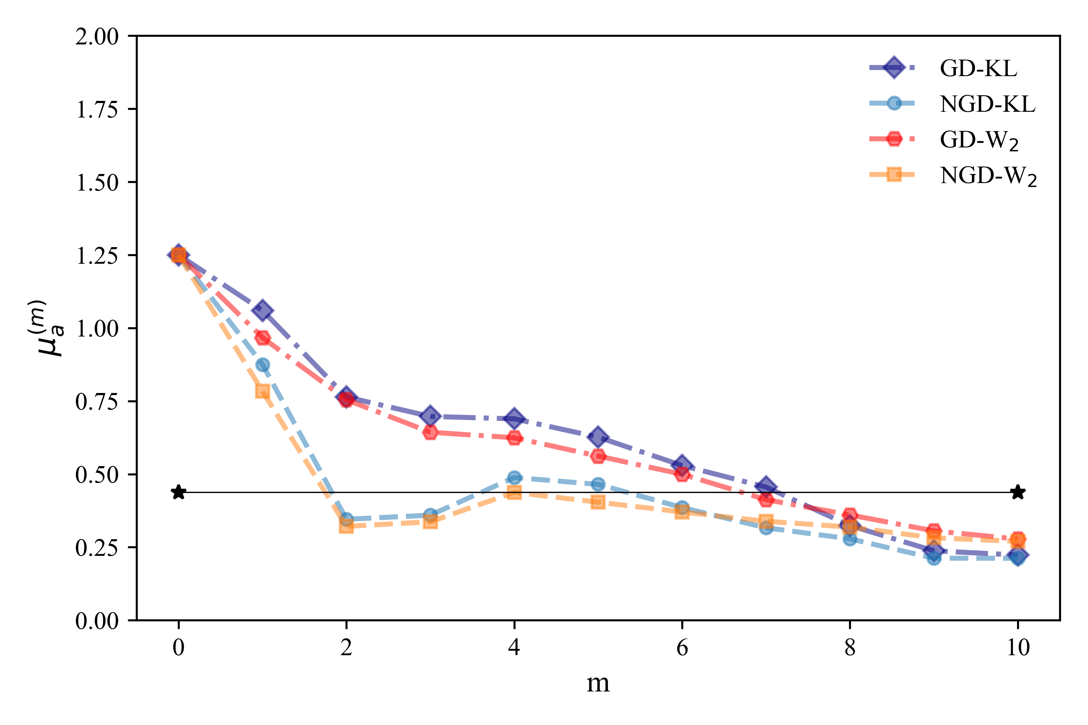
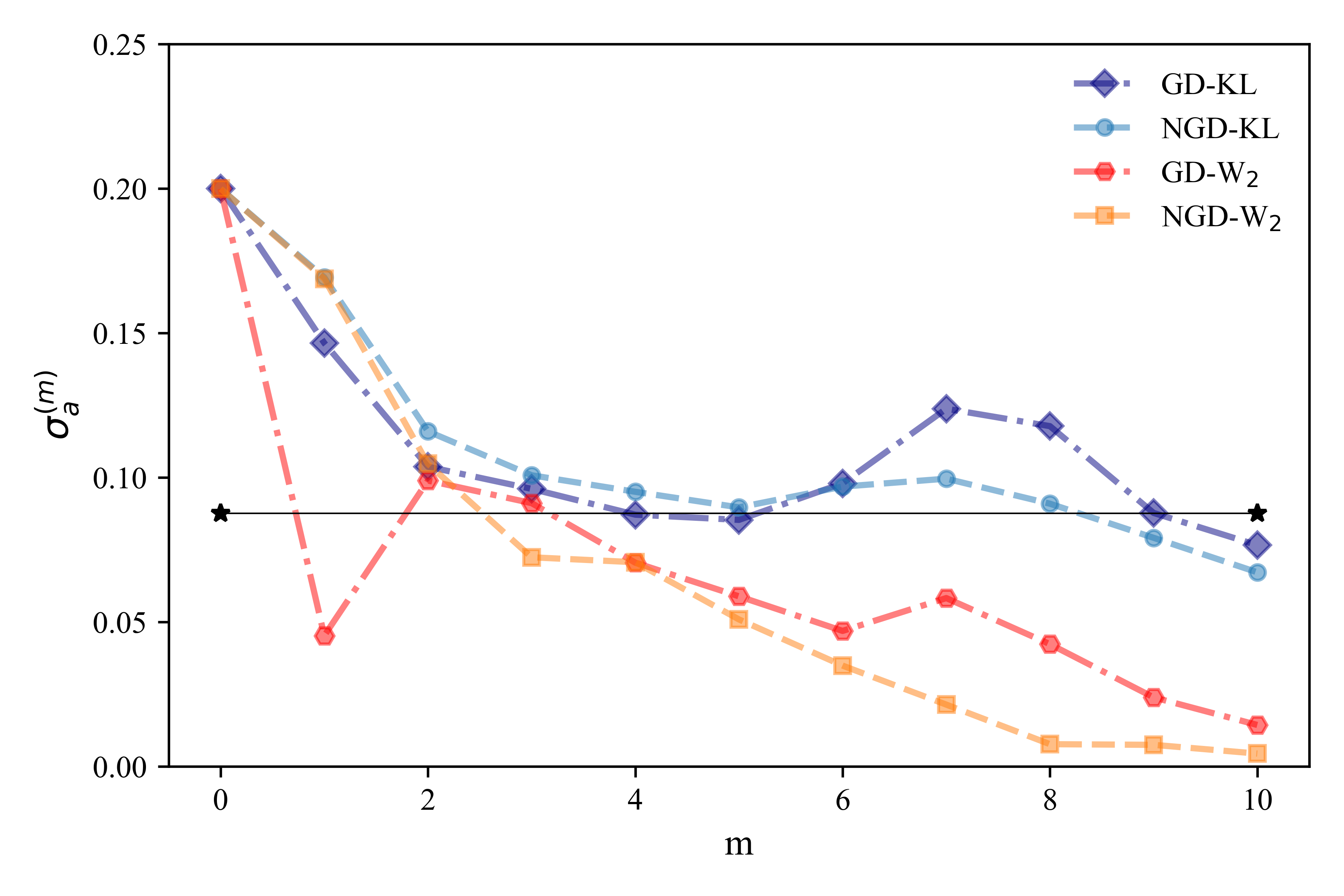
Figure 5: Estimation of meta-parameters $\boldsymbol{\varphi}=\{\mu_{a},\sigma_{a}\}$ for the Langevin equation with white noise. The parameters $\boldsymbol{\varphi}^{(m)}$ are plotted as function of the assimilation step $m$ for the four information-geometric optimization strategies: GD and NGD, for the KL and $W_{2}$ discrepancies. The simulation parameter values are set to $x_{0}^{\star}=1$, $\boldsymbol{\varphi}^{\star}=\{0.44,0.088\}$, $\boldsymbol{\varphi}^{(0)}=\{1.25,0.2\}$ , $\sigma_{\varepsilon}=0.1$, $N_{\text{meas}}=10$, $t_{N_{\text{meas}}}=2$, $\epsilon_{\text{KL}}=10^{-2}$, $N_{T}=18850$, $N_{B}=5632$, $N_{I}=1280$, and $N_{R}=47872$.

Like before, the number of iterations over the assimilation time window is smaller for NGD than for GD for both choices of loss function (fig. 6), albeit the difference is not as pronounced. The physics-driven parameterization of the statistical manifold yields an isotropic geometry of the loss function in the search area, which reduces the benefits of preconditioning. This is shown in fig. 7, where the KL and $W_{2}$ loss functions are plotted, at the first and last assimilation steps, as function of the meta-parameters $\boldsymbol{\varphi}$, also highlighting the true solution and the prior location. Although superficially similar throughout the assimilation process, the minor differences in the topology of the KL and W₂ loss functions are enough to prevent convergence for the KL loss function for a slightly worst choice of the prior (P₂ in the Figure), which results in divergence of the DA-MD procedure for both GD and NGD. This is because the KL divergence is more sensitive to numerical errors in the calculation of the integrals, especially for sharp or non-overlapping distributions, which mislead the direction of the search.

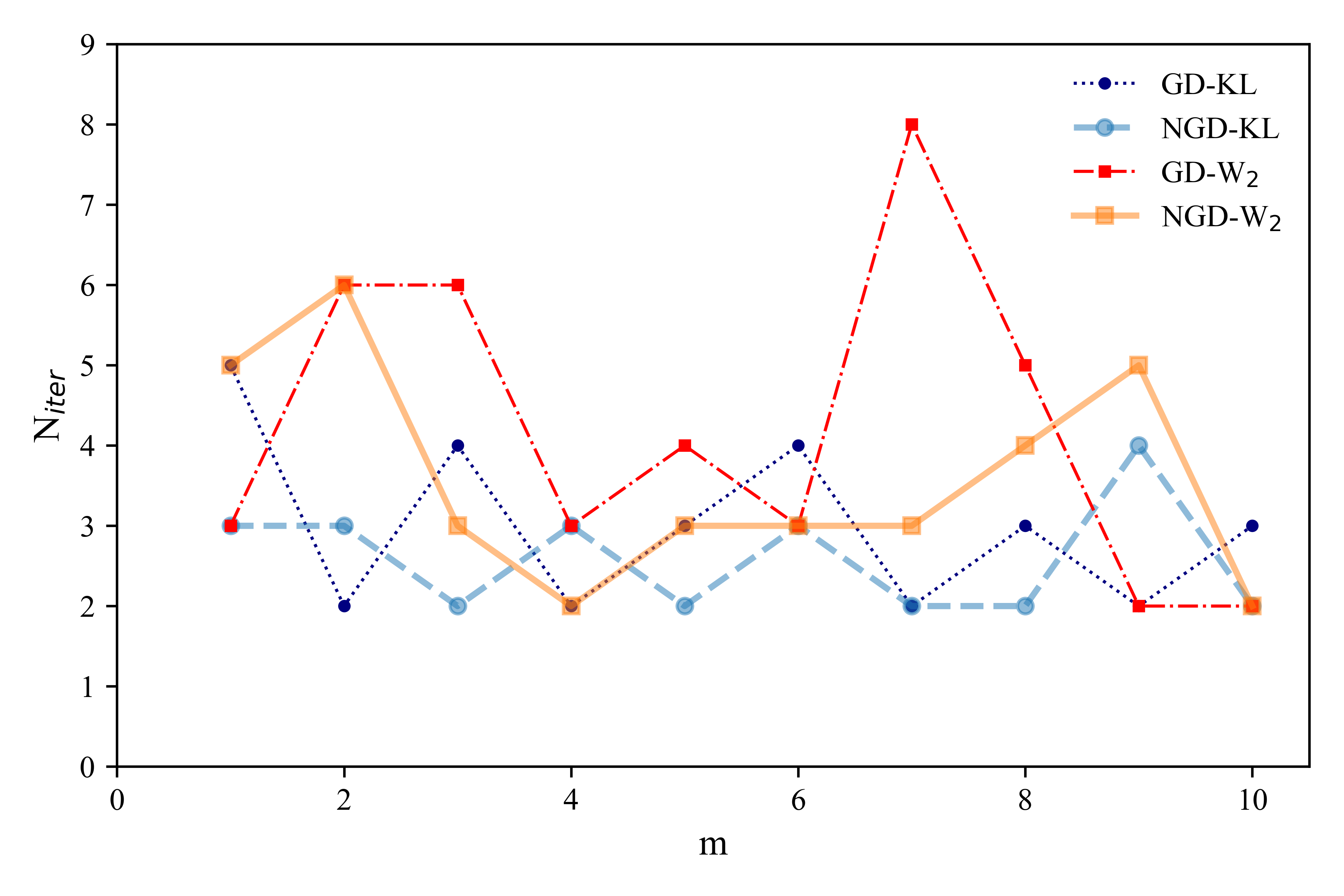
Figure 6: Number of iterations per assimilation step $m$ for the four information-geometric optimization strategies: GD and NGD, for the KL and $W_{2}$ discrepancies. The simulation parameter values are the same as in fig. 5.

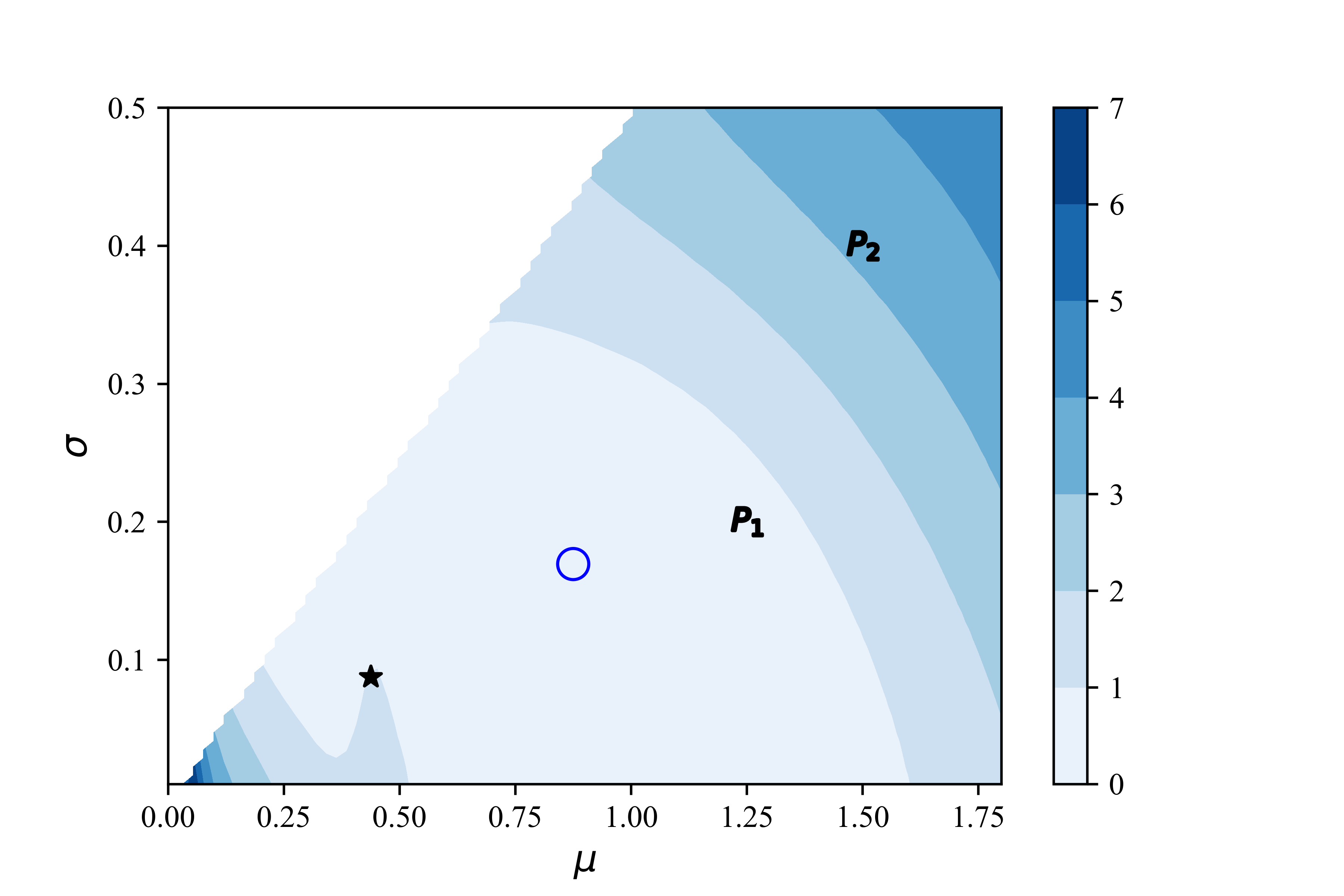
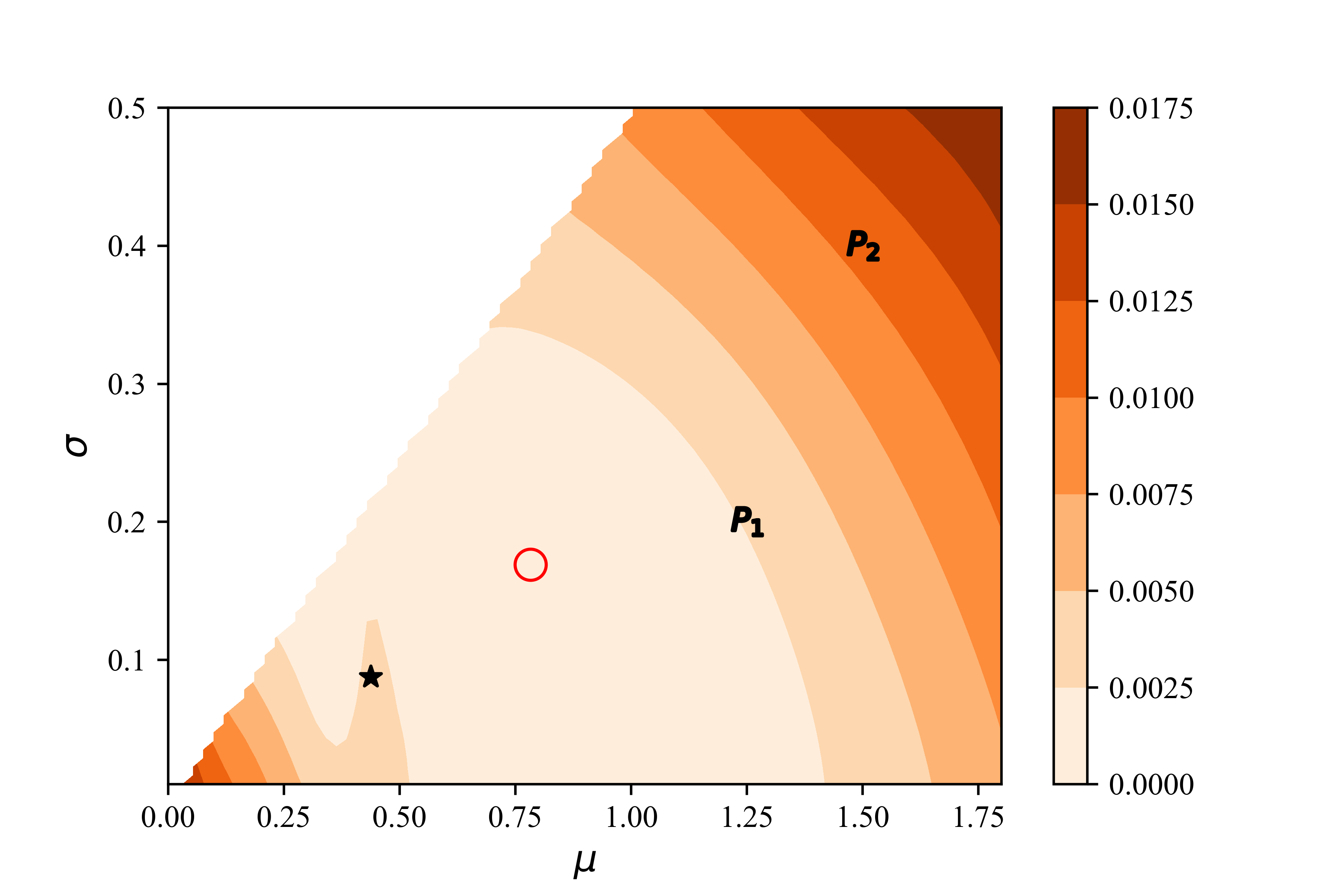
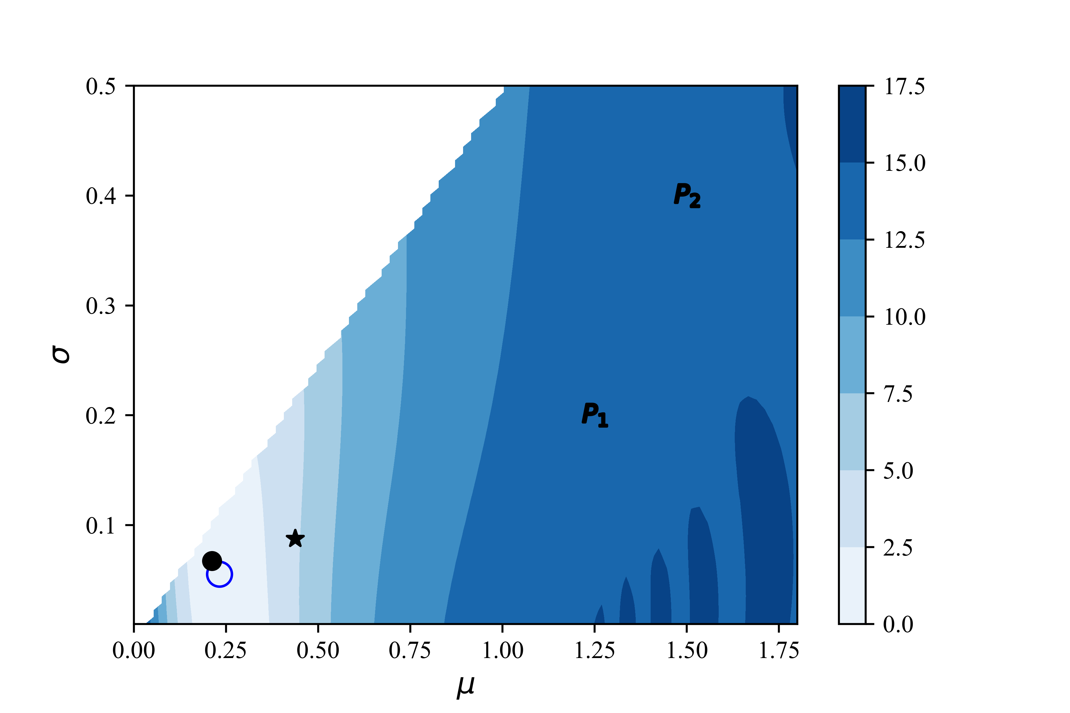
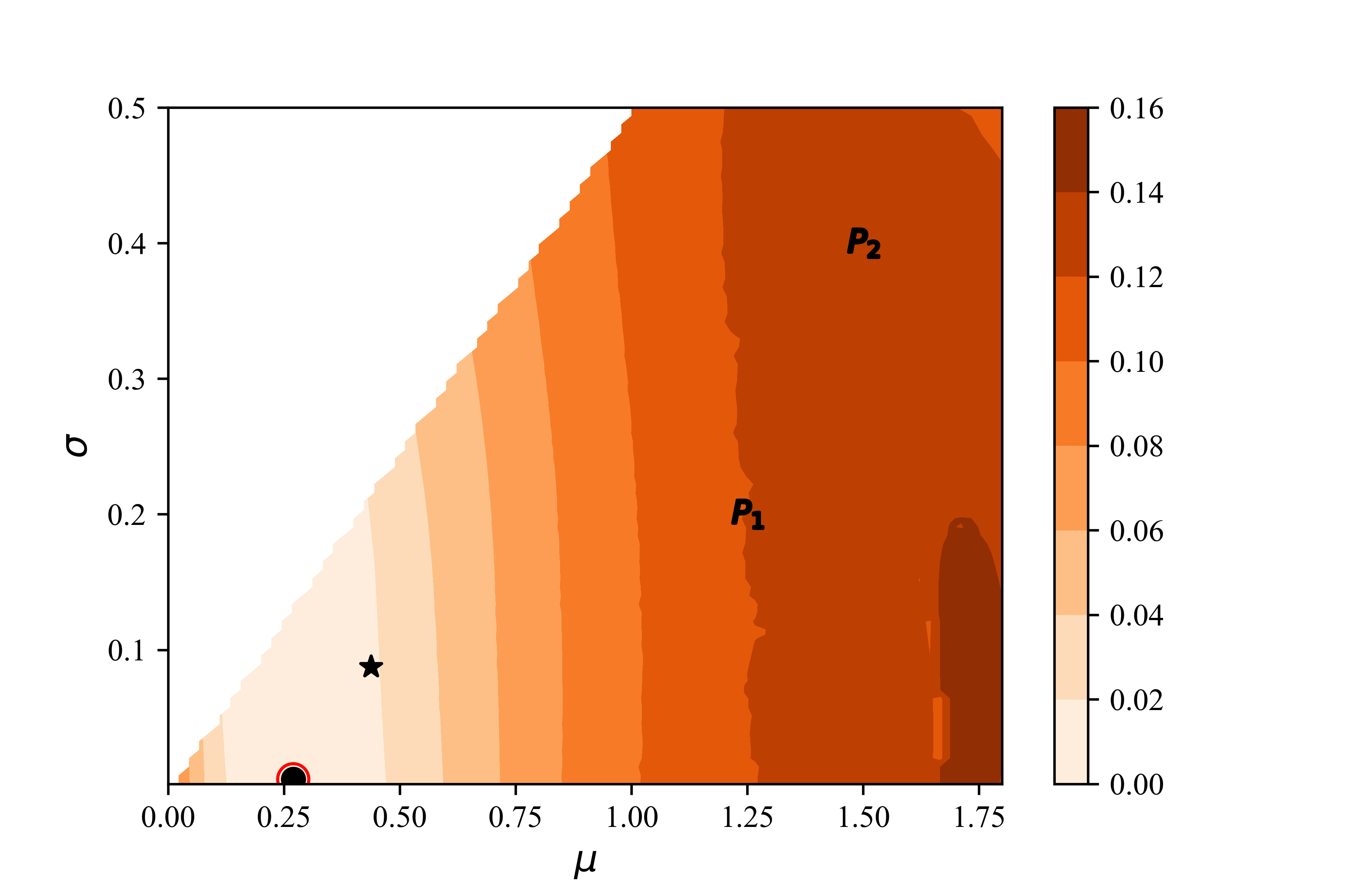
Figure 7: The KL (left column) and $W_{2}$ (right column) loss functions at the first ($m=1$, top row) and last ($m=N_{\text{meas}}$) steps of DA. The star indicates the true values of the meta-parameters (used to generate the synthetic reality). The points $P_{1}$ and $P_{2}$ indicates the priors $\boldsymbol{\varphi}^{(0)}$ for which the optimization of the KL loss function converges and fails to converge, respectively. The larger (empty) circles indicate the posterior parameters at the $m$th assimilation step, $\boldsymbol{\varphi}^{(m+1)}$, and the smaller (full) circles in the bottom row indicate $\boldsymbol{\varphi}^{(N_{\text{meas}}-1)}$. The blank region in all panels is to enforce almost surely the non-negativity of $a(t)$. The simulation parameter values are the same as in fig. 5.

The posterior NGD parameters $\boldsymbol{\varphi}^{(N_{\text{meas}})}$ are used to compute the posterior CDF and PDF of $x(t)$ in fig. 8. NGD yields accurate posteriors, with the $W_{2}$ optimization (8) performing better than the KL optimization (6). In order to highlight the accuracy of the DNN surrogate model, we show the finite-volume solution of the CDF equation (20) with $\boldsymbol{\varphi}=\boldsymbol{\varphi}^{(N_{\text{meas}})}$ and its corresponding PDF computed via numerical differentiation, and their DNN-based counterparts. In agreement within [17], we found the $W_{2}$ minimization to be more robust to the choice of the prior.

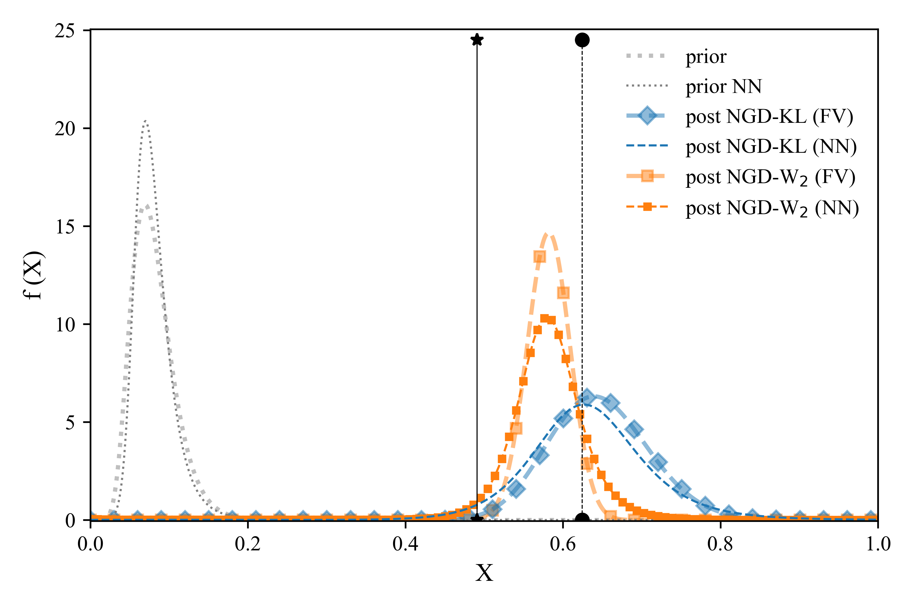
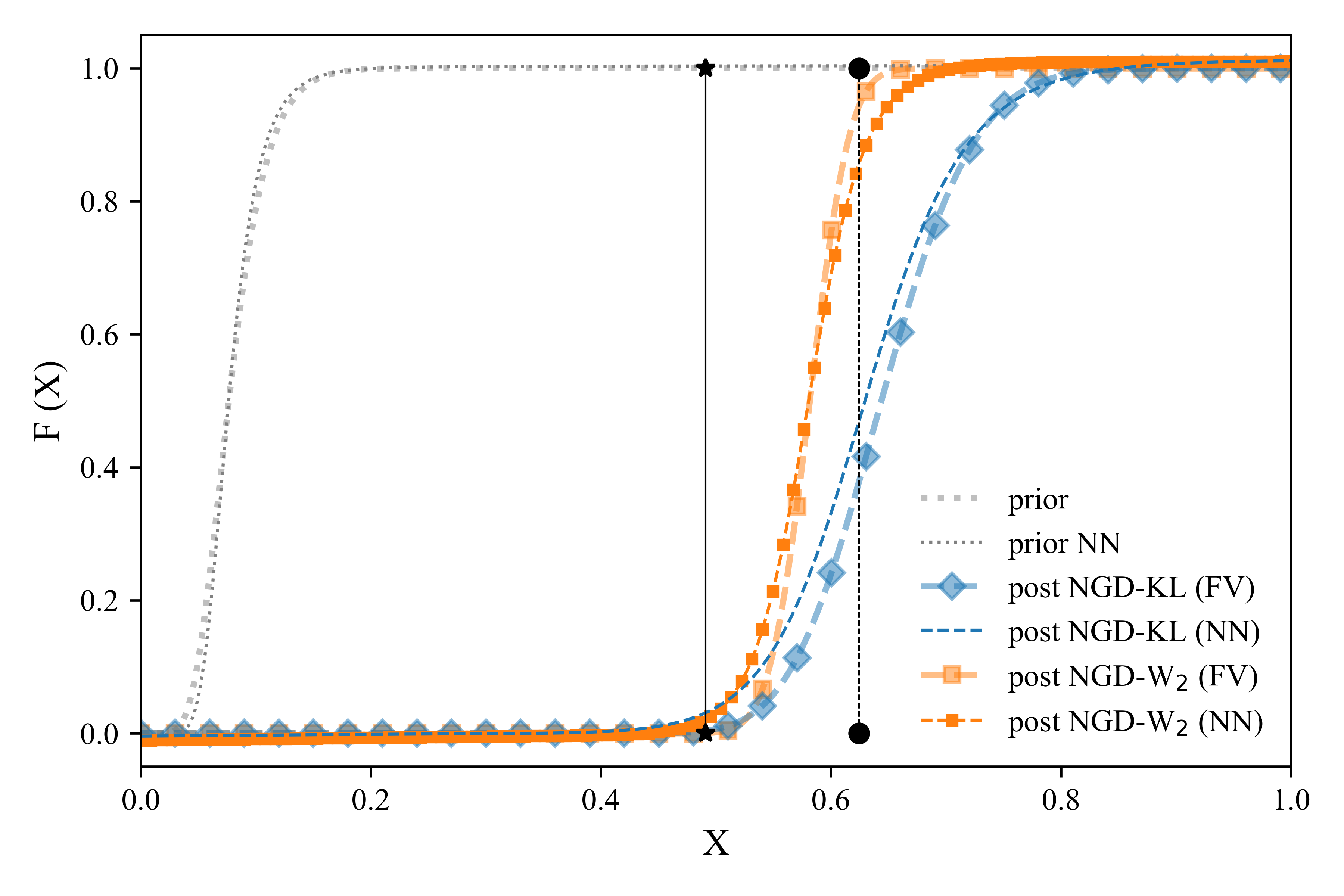
Figure 8: Prior and posterior distributions (PDFs on the left, and corresponding CDFs on the right) at time $t_{N_{\text{meas}}}$ obtained via NGD minimization for the KL and $W_{2}$ loss functions, with either the FV solution of the CDF equation (20) or its NN surrogate. Black stars and circles mark the exact value $x(t_{N_{\text{meas}}})$ and its noisy observation $x_{N_{\text{meas}}}$, respectively. The simulation parameter values are the same as in fig. 5.

Remark 4.2

An additional advantage of the $W_{2}$ loss function stems from its reliance on a CDF rather than a PDF that enters the KL loss function. CDFs are smoother and easier to compute as a solution of the CDF equation than PDFs, which are obtained by solving the PDF equation. This facilitates the generation of a training set and the training of a surrogate model. On the other hand, approximation of the solution to a CDF equation with a DNN surrogate possesses a potential challenge for the $W_{2}$ optimization, since (4) calls for invertible surrogate models. We overcome this difficulty by selecting a special structure for the DNN that guarantees automatic inversion, as detailed in section 3.

The computational cost of the different optimization strategies depends on the number of iterations (fig. 6); on the computational cost per iteration; and, in case of information-geometric optimization, on the cost of computing the tensor metrics. Since the function- and gradient-evaluations for this example are not expensive, the computational gain of having a smaller number of evaluations is not significant, and it is compensated by the additional cost of the calculation of the preconditioning matrices.

4.3 Langevin equation with colored noise

The dynamics of state variable $x(t)$ is described by (9) with $s(x(t);w(t),\boldsymbol{\theta})\equiv-a(t)x(t)$, where $a(t)=\mu_{a}+w(t)$ with $\mu_{a}\in\mathbb{R}^{+}$, and $w(t)$ is the derivative of an Ornstein–Uhlenbeck process characterized by the exponential auto-covariance function

$$C_{w}(t,\tau)=\frac{\sigma_{a}^{2}}{2\theta_{a}}\left[\text{e}^{-\theta_{a}|t-\tau|}+\text{e}^{-\theta_{a}(t+\tau)}\right],$$

with parameters $\sigma_{a}$ and $\theta_{a}\in\mathbb{R}^{+}$. By construction, the latter is also the auto-covariance function of $a(t)$, $C_{w}(t,\tau)=C_{a}(t,\tau)$. Taking the initial state $x_{0}$ to be deterministic, the stochastic solution of this problem depends on three meta-parameters $\boldsymbol{\varphi}=\{\mu_{a},\sigma_{a},\theta_{a}\}$. One realization of this solution, drawn from the distribution with the “true” meta-parameters $\boldsymbol{\varphi}^{\star}$, serves as ground truth for which observations $\hat{\mathbf{x}}$ are constructed in accordance with (10).

We show in section A.3 that the CDF $F(X;t)$ of $x(t)$ satisfies the CDF equation (11) with

$$\mathcal{U}(X,t;\boldsymbol{\varphi})=-\mu_{a}X+X\!\int_{0}^{t}\!\!C_{w}(t,\tau)\text{d}\tau\quad\text{and}\quad\mathcal{D}(X,t;\boldsymbol{\varphi})=X^{2}\!\int_{0}^{t}\!\!C_{w}(t,\tau)\text{d}\tau.$$ (21)

The FV solution of this equation and its DNN surrogate are used to assimilate observations $\hat{\mathbf{x}}$ via our information-geometric DA-MD framework. Similar to the case of white noise (section 4.2), we found the KL-based implementation of DA-MD to be less robust to the choice of the prior. Hence, only the $W_{2}$-based results are displayed below.

Figure 9 exhibits the convergence of the meta-parameters $\boldsymbol{\varphi}$ as function of the data assimilation step $m$. Since the $W_{2}$ loss function is relatively insensitive to the third meta-parameter $\theta_{a}$, we present the convergence results for $\tilde{\sigma}=\sqrt{\sigma^{2}/(2\theta_{a})}$ instead. Both GD-W₂ and NGD-W₂ converge after assimilation of about 20 observations, which are generated every $\Delta t=0.055$. NGD converges, for the given combination of observations and the prior, in fewer iterations over the assimilation window (fig. 9d) than GD.

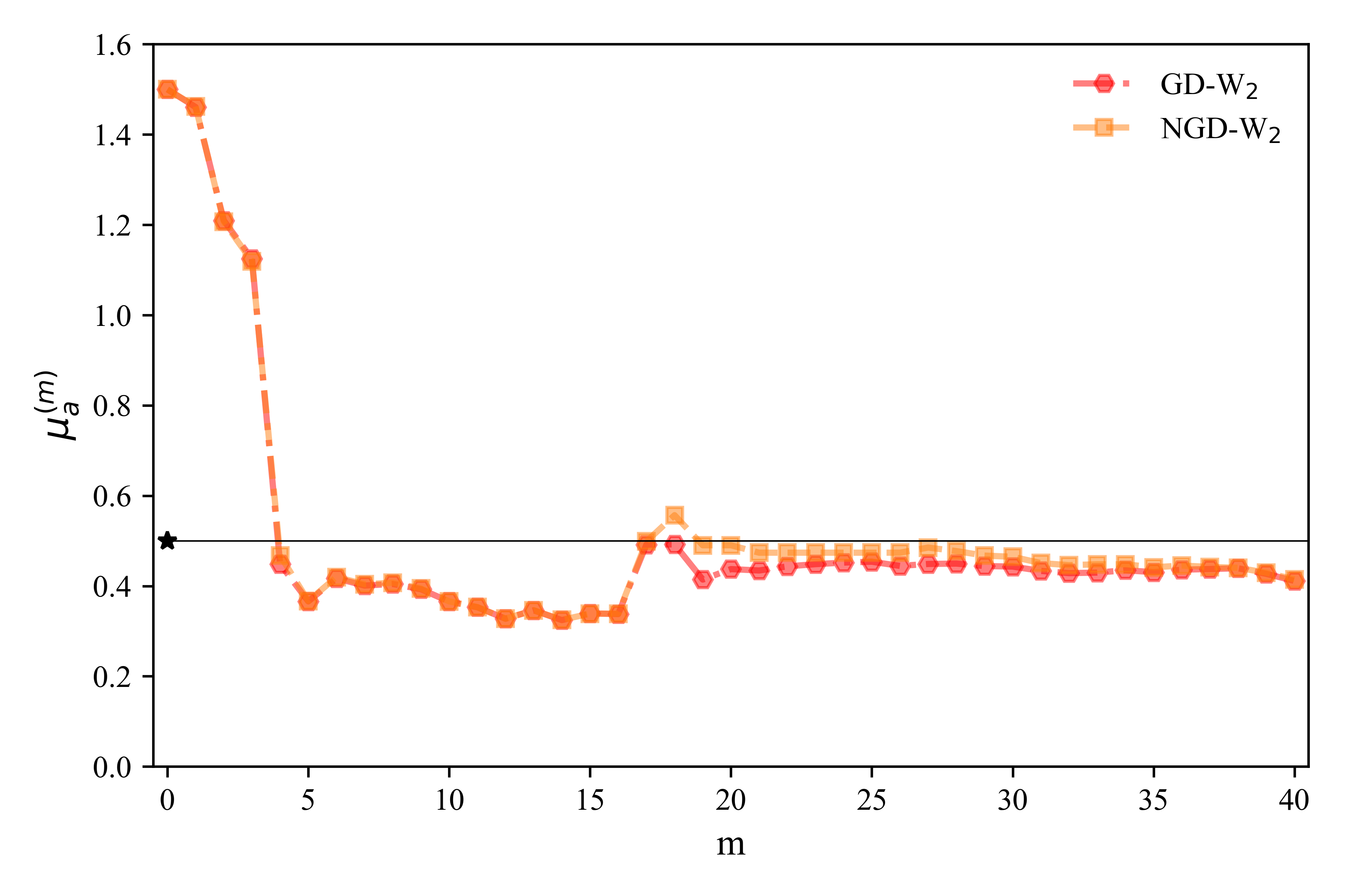
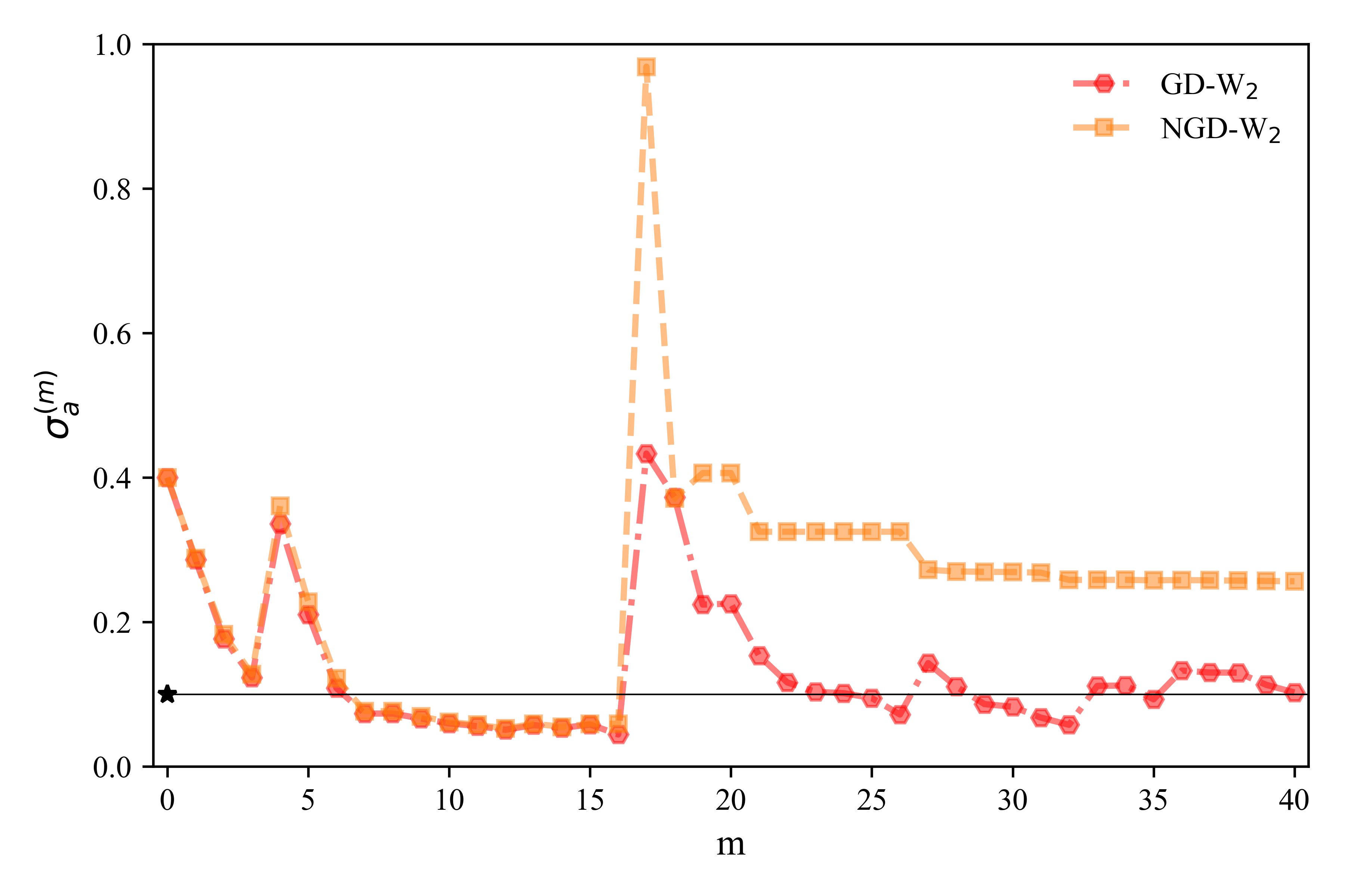
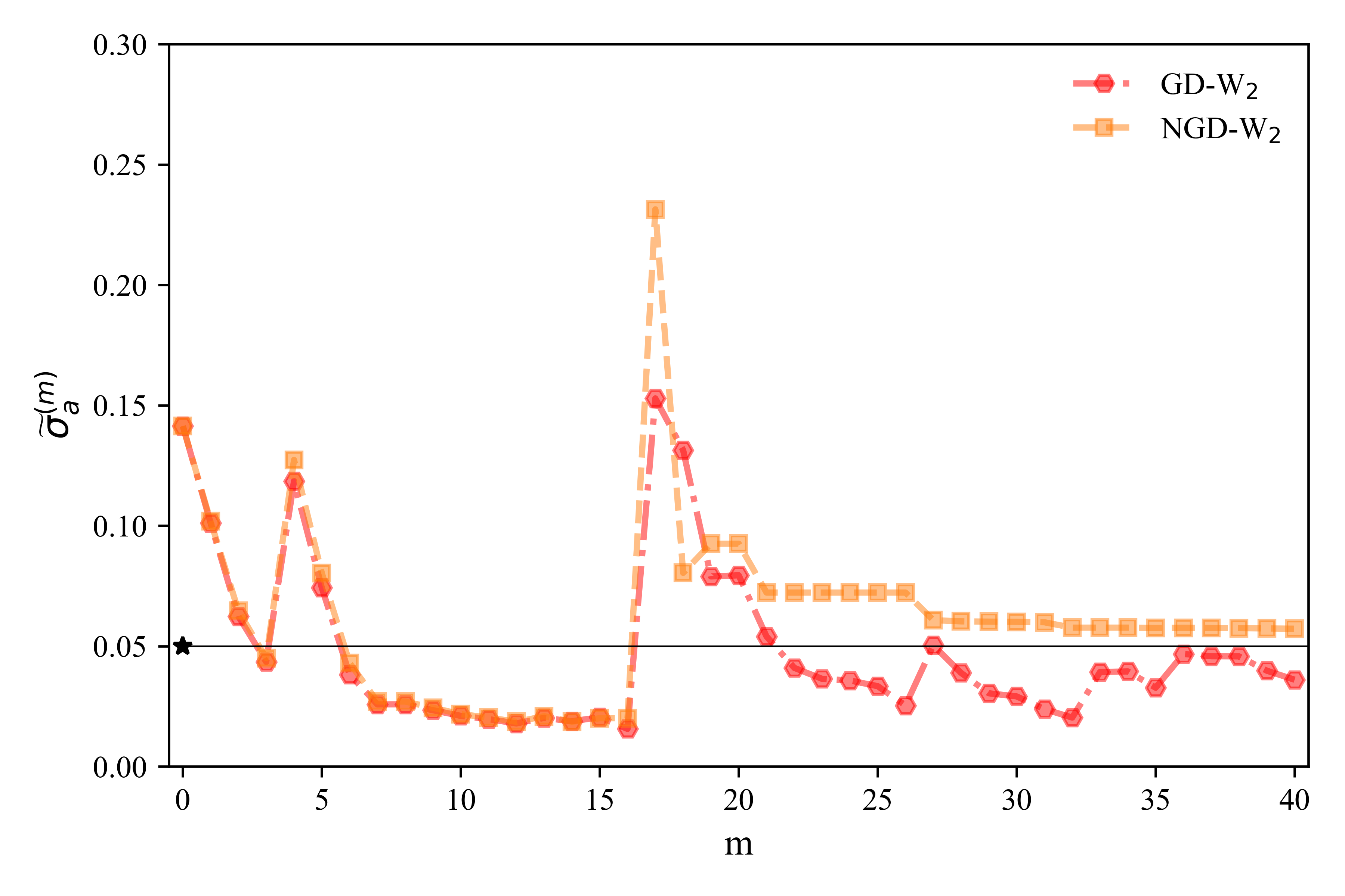
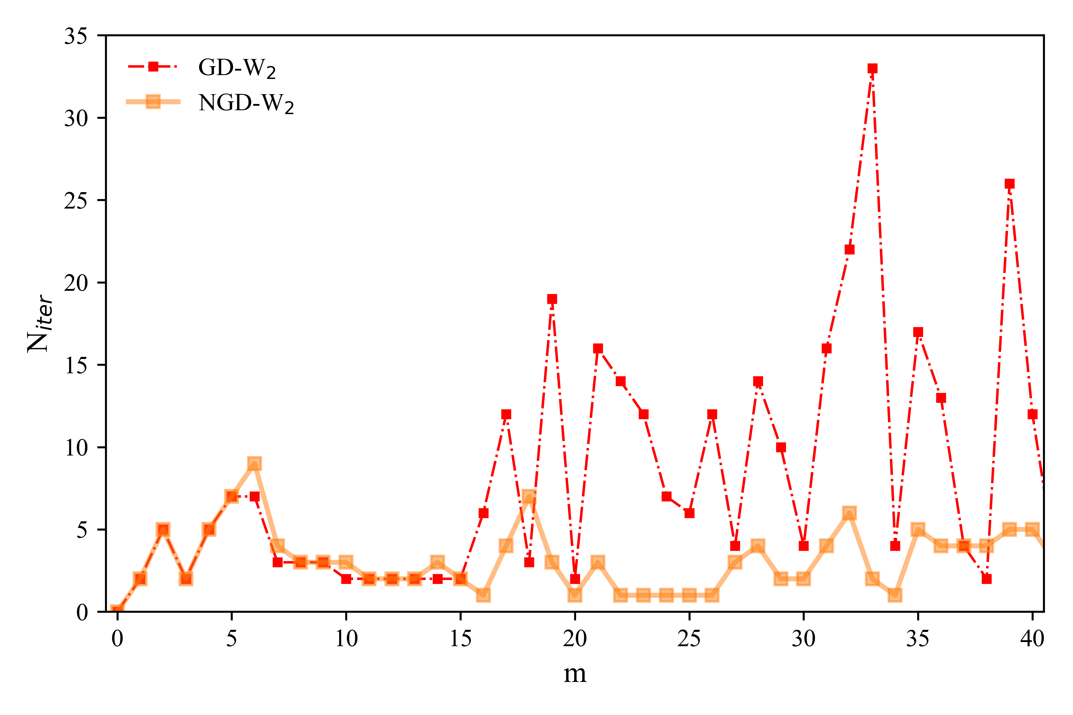
Figure 9: Estimation of meta-parameters $\boldsymbol{\varphi}=\{\mu_{a},\sigma_{a},\tilde{\sigma}=\sqrt{\sigma_{a}^{2}/(2\theta_{a})}\}$, as function of the assimilation step $m$, with GD and NGD for the $W_{2}$ loss functions. The bottom right panel shows the number of iterations per assimilation step for GD and NGD. The simulation parameter values are set to $x_{0}^{\star}=1$, $\boldsymbol{\varphi}^{*}=\{0.5,0.1,0.05\}$, $\boldsymbol{\varphi}^{(0)}=\{1.5,0.4,0.14\}$, $\sigma_{\varepsilon}=0.05$, $N_{\text{meas}}=41$, $t_{N_{\text{meas}}}=2.2$, $\epsilon_{\text{KL}}=10^{-2}$, $N_{T}=13550$, $N_{B}=29282$, $N_{I}=6655$, $N_{R}=248897$.

In fig. 10, we present the posterior PDF and CDF of the state $x(t)$ at the final assimilation time $t_{N_{\text{meas}}}$. The CDF is computed as a FV solution of the CDF equation with meta-parameters $\boldsymbol{\varphi}^{(N_{\text{meas}})}$, and the PDF as its derivative. Observations $\hat{\mathbf{x}}$ are assimilated, alternatively, via the GD-W₂ and NGD-W₂ optimization strategies. Both approaches yield posterior distributions that are close to the true state, with negligible differences between NGD-W₂ and GD-W₂. The use of the FV solution of the CDF equation leads to a slightly wider posterior than the reliance on its DNN surrogate does, possibly because of numerical diffusion.

Although not shown here, we found the KL- and $W_{2}$-based loss functions at at the first and later assimilation steps to be smooth and not significantly different from each other. Yet, similar to the example in section 4.2, the differences are sufficient to prevent convergence in the KL case for poor choices of the prior.

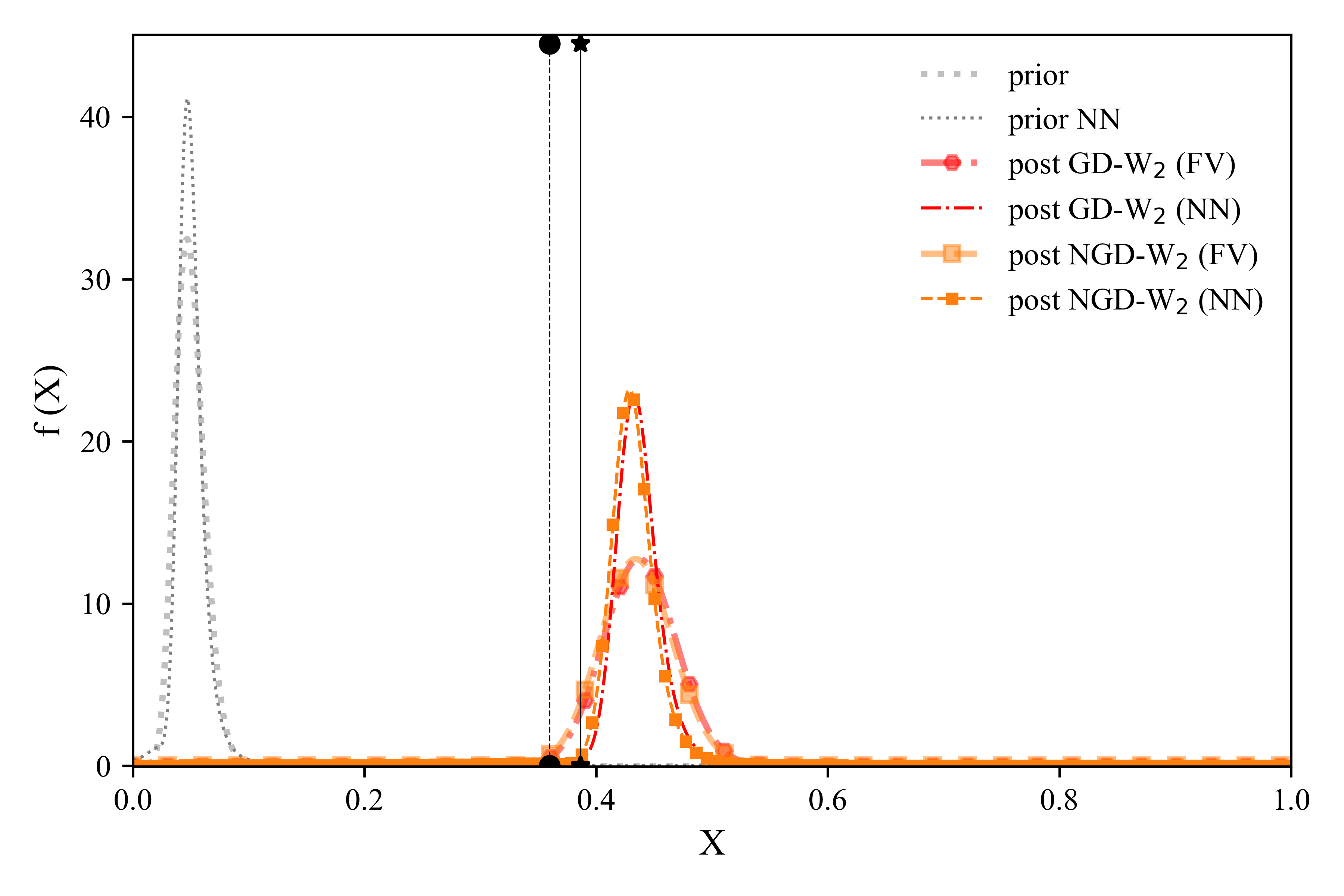
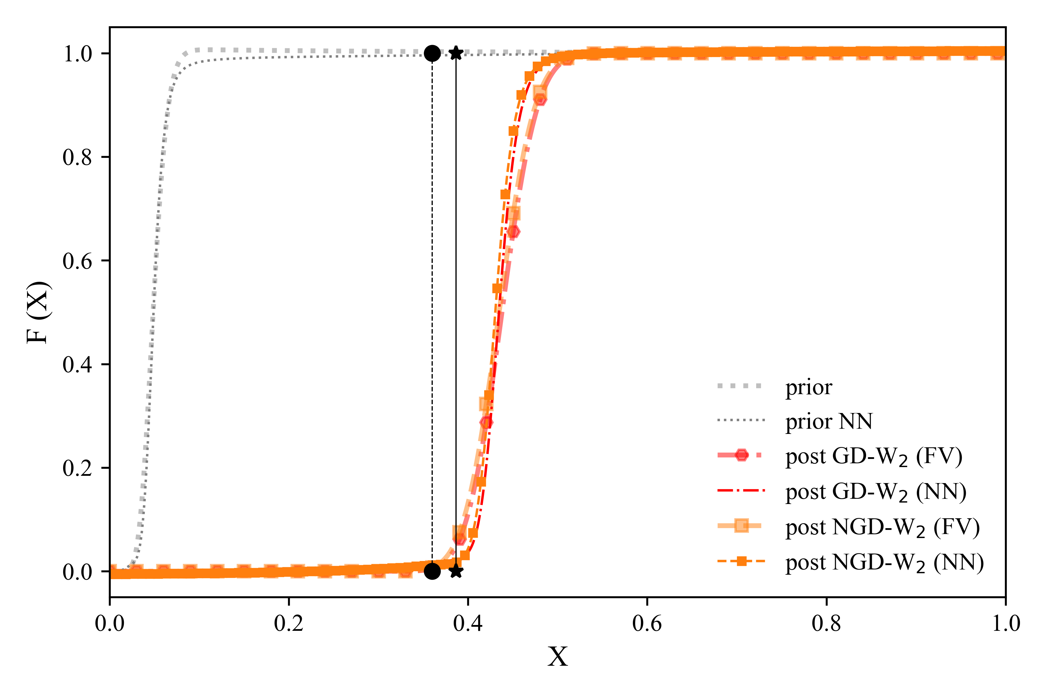
Figure 10: Prior and posterior distributions at time $t_{N_{\text{meas}}}$ (both PDFs, on the left, and CDFs, on the right) obtained via GD-W₂ and NGD-W₂ minimization for the Langevin equation with colored noise. For each distribution, both the FV solution and NN approximation are shown. Black stars and circles mark the exact value $x(t_{N_{\text{meas}}})$ and its noisy observation $x_{N_{\text{meas}}}$, respectively. The simulation parameter values are the same as in fig. 9.

5 Discussion and Conclusions

We presented an information-geometric implementation of DA-MD, which yields computationally efficient data assimilation and parameter estimation for nonlinear problems with non-Gaussian system states. The forecast step is performed by employing the MD, an uncertainty propagation technique that yields a deterministic evolution equation for the CDF (or, equivalently, the PDF) of the state. This equation maps a set of meta-parameters (statistical properties of the random inputs) onto the system-state distribution, and defines a parameter space for a dynamic manifold of distributions. The analysis step is performed on this statistical manifold; it is formulated as sequential minimization of the discrepancy between an observational distribution and a predictive posterior distribution obeying the CDF equation with unknown (posterior) parameters. The observational PDF is the Bayesian posterior obtained as the product of the data model (i.e., the likelihood function) and the prior distribution obeying the CDF equation with the parameters from the previous assimilation step.

Reliance on statistical discrepancy measures—the Kullback-Leibler divergence and the $L_{2}$ Wasserstein distance—confers exploitable geometric properties to the manifold of distributions. Specifically, it enables the use of NGD, an efficient optimization technique. Our numerical experiments revealed the $W_{2}$-based DA-MD to be more robust to the choice of a prior than its KL-based counterpart.

For one-dimensional (univariate) distributions, $W_{2}$ is defined in terms of system-state CDFs, and KL in terms of corresponding PDFs. This argues in favor of the $W_{2}$-based DA-MD, since CDFs are smoother and numerical solution of CDF equations is easier. This facilitates the use of invertible DNNs as a surrogate model in the probabilistic space to facilitate and accelerate optimization and calculation of the geometric metric tensors.

Future work will focus on the identification of ambiguity sets and their dynamics on statistical manifolds [25], their evolution and their update with observations. We also plan to explore the use of different data models, the impact of alternative parameterizations of a statistical manifold on DA-MD performance, and the latter’s implications for sensitivity analysis.

Appendix A CDF equation for the stochastic ODE

We summarize the MD for the three test problems from section 4. The original derivations can be found in [3], [45] and [6], respectively. The first two results are exact, whereas the third one is approximate and has been verified against Monte Carlo simulations in [5, 6].

A.1 Stochastic ODE with random initial conditions

We consider (9) with a smooth deterministic function $s(x,t;\boldsymbol{\theta})$; random initial state $x_{0}\in\mathbb{R}$ is described by a given CDF $F_{0}(X;\boldsymbol{\varphi}_{0})$ with statistical parameters $\boldsymbol{\varphi}_{0}$. To derive an equation for $F(X;t)$, the CDF of $x(t)$, we first define the raw CDF $\Pi=\mathcal{H}(X-x(t))$ whose ensemble mean is $\langle\Pi(X;t)\rangle=F(X;t)$. Next, we multiply (9) by $-\partial\Pi/\partial X$ and use the properties of the Heaviside function $\mathcal{H}(\cdot)$ to obtain

$$\frac{\partial\Pi}{\partial t}+s(X,t;\boldsymbol{\theta})\frac{\partial\Pi}{\partial X}=0.$$ (22)

Since $s(\cdot)$ is deterministic, the ensemble average of (22) yields (16), which is a special case of (11) with $\mathcal{U}=s(X,t;\boldsymbol{\theta})$ and $\mathcal{D}=0$.

The derivation of a corresponding PDF equation starts with the definition of a raw PDF $\pi=\delta(X-x(t))$, where $\delta(\cdot)$ is the Dirac distribution. A procedure similar to above yields [3, sec. 2.1]

$$\frac{\partial f}{\partial t}+\frac{\partial s(X,t;{\boldsymbol{\theta}})f}{\partial X}=0.$$ (23)

This equation can also be obtained by differentiation of (16) with respect to $X$.

A.2 MD for the Langevin equation with white noise

Consider a Langevin equation, (9) with $s(x;w)\equiv s_{d}(x,t)+s_{w}(x,t)w(t)$ where $w(t)$ is a white standard Gaussian process (with zero mean and unit variance). The deterministic functions $s_{d}$ and $s_{w}$ are such that $s(x;w)$ is integrable with respect to $t$ in the mean square sense [45, Sec. 4.1]. The derivation of a PDF equation for $x(t)$ is relatively straightforward, and leads to the Fokker-Planck equation (a.k.a. Kolmogorov’s forward equation) [45, Sec. 4.9]

$$\frac{\partial f}{\partial t}+\frac{\partial\,s_{d}(X,t)f}{\partial X}=\frac{1}{2}\frac{\partial^{2}s_{w}^{2}(X,t)f}{\partial X^{2}},$$ (24)

It is formally valid if $f(X;t)$ is well-behaved at infinity, and is subject to initial and boundary conditions condition $f(X;0)=f_{0}(x)$ and $f(\pm\infty;t)=0$.

An equivalent CDF version of the Fokker-Planck equation (24) can be obtained via integration of (24) over $X\in\Omega$

$$\frac{\partial F}{\partial t}+s_{d}(X,t)\frac{\partial F}{\partial X}=\frac{1}{2}\frac{\partial}{\partial X}\left(s_{w}^{2}(X,t)\frac{F}{\partial X}\right),$$ (25)

subject to $F(x;0)=F_{0}(X)$, $F(X_{\text{min}},t)=0$, and $F(X_{\text{max}},t)=1$.

In (19), $s(x;w)=-a(t)x(t)$ where the random process $a(t)$ has the constant mean $\mu_{a}$ and standard deviation $\sigma_{a}$. This translates into $s_{d}(x,t)=-\mu_{a}x$ and $s_{w}=-\sigma_{a}x$, so that the coefficients $\mathcal{U}$ and $\mathcal{D}$ in (11) become $\mathcal{U}=-\mu_{a}X$ and $\mathcal{D}=(\sigma_{a}^{2}/2)X^{2}$, with $\boldsymbol{\varphi}=\{\mu_{a},\sigma_{a}\}$.

A.3 MD for the Langevin equation with colored noise

Consider (9) with $s(x;w)\equiv-a(t)x(t)$, where $a(t)=\mu_{a}+w(t)$ and $w(t)$ is a correlated standard Gaussian process. The MD for stochastic/random (Langevin) ODEs with temporally correlated forcings requires closure approximations. These include the semi-local approximation  [5, 6], which compares favorably with Monte Carlo simulations and a local closure approximation in terms of both accuracy and computational efficiency. For the sake of completeness, we summarize the derivation of the PDF equation and its semi-local closure approximation for the specific form of the Langevin equation described above. We start by deriving an equation for the raw PDF $\pi(X,t)=\delta(X-x(t))$, whose ensemble mean is the PDF, $f(X;t)=\langle\pi\rangle$. Multiplying our ODE by $-\partial\pi/\partial X$ and using the properties of the Dirac delta function $\delta(\cdot)$, we obtain

$$\frac{\partial\pi}{\partial t}+a(t)\frac{\partial\pi}{\partial X}=0.\qquad s(X,t)=\langle s(X,t)\rangle+s^{\prime}(X,t;w);\quad\langle s\rangle=-\mu_{a}X,s^{\prime}=-w(t)X$$ (26)

We use the Reynolds decomposition $\mathcal{A}=\langle\mathcal{A}\rangle+\mathcal{A}^{\prime}$ to represent relevant random processes $\mathcal{A}$ as the sums of their ensemble means $\langle\mathcal{A}\rangle$ and zero-mean fluctuations around these means, $\mathcal{A}^{\prime}$. Since $\pi=f+\pi^{\prime}$, taking the ensemble mean of this equation yields an unclosed equation for the PDF $f(X;t)$,

$$\frac{\partial f}{\partial t}+\mu_{a}\frac{\partial f}{\partial X}+\frac{\partial\langle w^{\prime}(t)\pi^{\prime}(X,t)\rangle}{\partial X}=0,\qquad\text{subject to}\quad f(X;0)=f_{0}.$$ (27)

A closure approximation is needed to render the cross-correlation term $\langle w^{\prime}(t)\pi^{\prime}(X,t)\rangle$ computable. Subtracting (27) from (26), we obtain an equation for random fluctuations $\pi^{\prime}(X,t)$,

$$\frac{\partial\pi^{\prime}}{\partial t}+\mu_{a}\frac{\partial\pi^{\prime}}{\partial X}=\frac{\partial(\langle s^{\prime}(X,t)\pi^{\prime}(X,t)\rangle-s^{\prime}\pi)}{\partial X},\qquad\text{subject to}\quad\pi^{\prime}(X,t=0)=0.$$ (28)

The deterministic Green’s function for (28), $G(X,t;\Xi,\tau)$, is a solution of

$$\frac{\partial G}{\partial\tau}+\mu_{a}\frac{\partial G}{\partial\Xi}=-\delta(X-\Xi)\delta(t-\tau)$$ (29)

with homogeneous initial (at $\tau=t$) and boundary conditions at infinity. Its analytical solution, obtained, e.g., via the method of characteristics, is $G(X,t;\Xi,\tau)=\mathcal{H}(t-\tau)\delta(X-\Xi\exp(-\mu_{a}(t-\tau)))$. Hence, the path-wise solution of (28) is

$$\pi^{\prime}(X,t)=\int_{0}^{t}\int_{-\infty}^{\infty}G(X,t;\Xi,\tau)\frac{\partial}{\partial\Xi}\left[\langle w^{\prime}(\Xi,\tau)\pi^{\prime}(\Xi,\tau)\rangle-w^{\prime}(\Xi,\tau)\pi(\Xi,\tau)\right]\text{d}\tau\text{d}\Xi.$$ (30)

A closure approximation for $\langle w^{\prime}(t)\pi^{\prime}(X,t)\rangle$ is constructed by multiplying (30) with $w^{\prime}(t)$, taking the ensemble mean, and neglecting the third-order correlation term,

$$\langle w^{\prime}(X,t)\pi^{\prime}(X,t)\rangle=-\int_{0}^{t}\int_{-\infty}^{\infty}G(X,t;\Xi,\tau)\frac{\partial}{\partial\Xi}\left(C_{w}(X,t;\Xi,\tau)f(\Xi,\tau)\right)\text{d}\Xi\text{d}\tau,$$ (31)

where $C_{w}(X,t;\Xi,\tau)=\langle w^{\prime}(X,t)w^{\prime}(\Xi,\tau)\rangle$ is the auto-covariance of the random noise $w(t)$. Substituting this expression into (27) yields a nonlocal (integro-differential) PDF equation. Accounting for the analytical expression for $G$, (31) is approximated semi-locally as

$$\langle w^{\prime}(X,t)\pi^{\prime}(X,t)\rangle=-Xf(X,t)\int_{0}^{t}C_{w}(t,\tau)\text{d}\tau-X^{2}\frac{\partial f(X,t)}{\partial X}\int_{0}^{t}C_{w}(t,\tau)\text{d}\tau.$$ (32)

This yields the closed CDF equation (11) with (21). If $w(t)$ were white noise, i.e., if $C_{w}(t,\tau)=\delta(t-\tau)$, then the resulting PDF equation would reduce to the Fokker-Planck equation.

References

- [1] H. Risken. The Fokker-Planck Equation. Springer, 1996.
- [2] L. D. Landau and E. M. Lifshitz. Statistical Physics, Part 1. Elsevier, Amsterdam, 1980.
- [3] D. M. Tartakovsky and P. A. Gremaud. Method of distributions for uncertainty quantification. In R. Ghanem, D. Higdon, and H. Owhadi, editors, Handbook of Uncertainty Quantification, pages 763–783. Springer, 2015.
- [4] P. Wang, A. M. Tartakovsky, and D. M. Tartakovsky. Probability density function method for Langevin equations with colored noise. Phys. Rev. Lett., 110(14):140602, 2013.
- [5] D. A. Barajas-Solano and A. M. Tartakovsky. Probabilistic density function method for nonlinear dynamical systems driven by colored noise. Phys. Rev. E, 93(5):052121, 2016.
- [6] T. Maltba, P. A. Gremaud, and D. M. Tartakovsky. Nonlocal PDF methods for Langevin equations with colored noise. J. Comput. Phys., 367:87–101, 2018.
- [7] C. K. Wikle and L. M. Berliner. A Bayesian tutorial for data assimilation. Physica D, 230(1-2):1–16, 2007.
- [8] F. Boso and D. M. Tartakovsky. Learning on dynamic statistical manifolds. Proc. Roy. Soc. A, 476(2239):20200213, 2020.
- [9] S. Brooks, A. Gelman, G. Jones, and X.-L. Meng. Handbook of Markov Chain Monte Carlo. CRC Press, 2011.
- [10] G. Evensen. Data assimilation: the ensemble Kalman filter. Springer, 2009.
- [11] M. S. Arulampalam, S. Maskell, N. Gordon, and T. Clapp. A tutorial on particle filters for online nonlinear/non-Gaussian Bayesian tracking. IEEE Trans. Sign. Proces., 50(2):174–188, 2002.
- [12] F. Boso, S. V. Broyda, and D. M. Tartakovsky. Cumulative distribution function solutions of advection-reaction equations with uncertain parameters. Proc. R. Soc. A, 470(2166):20140189, 2014.
- [13] F. Boso and D. M. Tartakovsky. Data-informed method of distributions for hyperbolic conservation laws. SIAM J. Sci. Comput., 42(1):A559–A583, 2020.
- [14] S. Kullback. Information theory and statistics. Courier Corporation, 1997.
- [15] D. M. Blei, A. Kucukelbir, and J. D. McAuliffe. Variational inference: A review for statisticians. J. Am. Stat. Assoc., 112(518):859–877, 2017.
- [16] G. Peyré and M. Cuturi. Computational optimal transport: With applications to data science. Found. Trends Mach. Learn., 11(5-6):355–607, 2019.
- [17] Y. Chen and W. Li. Wasserstein natural gradient in statistical manifolds with continuous sample space. arXiv preprint arXiv:1805.08380, 2018.
- [18] F. Kunstner, P. Hennig, and L. Balles. Limitations of the empirical Fisher approximation for natural gradient descent. In Advances in Neural Information Processing Systems, pages 4156–4167, 2019.
- [19] C. Villani. Topics in optimal transportation, volume 58. American Mathematical Society, 2003.
- [20] V. M. Panaretos and Y. Zemel. Statistical aspects of Wasserstein distances. Ann. Rev. Stat. Appl., 6:405–431, 2019.
- [21] C. Frogner, C. Zhang, H. Mobahi, M. Araya, and T. A. Poggio. Learning with a Wasserstein loss. In Advances in Neural Information Processing Systems, pages 2053–2061, 2015.
- [22] M. Arjovsky, S. Chintala, and L. Bottou. Wasserstein GAN. arXiv preprint arXiv:1701.07875, 2017.
- [23] J. Neyman and E. L. Scott. Consistent estimates based on partially consistent observations. Econometrica, pages 1–32, 1948.
- [24] P. M. Esfahani and D. Kuhn. Data-driven distributionally robust optimization using the Wasserstein metric: Performance guarantees and tractable reformulations. Math. Progr., 171(1-2):115–166, 2018.
- [25] F. Boso, D. Boskos, J. Cortés, S. Martínez, and D. M. Tartakovsky. Dynamics of data-driven ambiguity sets for hyperbolic conservation laws with uncertain inputs. arXiv:2003.06735, 2020.
- [26] Y. Ollivier, L. Arnold, A. Auger, and N. Hansen. Information-geometric optimization algorithms: A unifying picture via invariance principles. J. Mach. Learn. Res., 18(1):564–628, 2017.
- [27] Y. Li, Y. Cheng, X. Li, H. Wang, X. Hua, and Y. Qin. Bayesian nonlinear filtering via information geometric optimization. Entropy, 19(12):655, 2017.
- [28] W. Li and G. Montúfar. Natural gradient via optimal transport. Inform. Geom., 1(2):181–214, 2018.
- [29] Y. Ollivier. Online natural gradient as a Kalman filter. El. J. Stat., 12(2):2930–2961, 2018.
- [30] Y. Ollivier. The Extended Kalman Filter is a natural gradient descent in trajectory space. arXiv preprint arXiv:1901.00696, 2019.
- [31] A. Takatsu. Wasserstein geometry of Gaussian measures. Osaka J. Math., 48(4):1005–1026, 2011.
- [32] L. Malagò, L. Montrucchio, and G. Pistone. Wasserstein Riemannian geometry of positive definite matrices. arXiv preprint arXiv:1801.09269, 2018.
- [33] S.-I. Amari, R. Karakida, and M. Oizumi. Information geometry connecting Wasserstein distance and Kullback–Leibler divergence via the entropy-relaxed transportation problem. Information Geom., 1(1):13–37, 2018.
- [34] M. Cuturi. Sinkhorn distances: Lightspeed computation of optimal transport. In Advances in neural information processing systems, pages 2292–2300, 2013.
- [35] F. Boso, A. Marzadri, and D. M. Tartakovsky. Probabilistic forecasting of nitrogen dynamics in hyporheic zone. Water Resour. Res., 54(7):4417–4431, 2018.
- [36] A. A. Alawadhi, F. Boso, and D. M. Tartakovsky. Method of distributions for water-hammer equations with uncertain parameters. Water Resour. Res., 54(11):9398–9411, 2018.
- [37] A. Guzman. Derivatives and integrals of multivariable functions. Springer, 2012.
- [38] M. Raissi, P. Perdikaris, and G. E. Karniadakis. Physics-informed neural networks: A deep learning framework for solving forward and inverse problems involving nonlinear partial differential equations. J. Comput. Phys., 378:686–707, 2019.
- [39] A. Gupta, N. Shukla, L. Marla, A. Kolbeinsson, and K. Yellepeddi. How to incorporate monotonicity in deep networks while preserving flexibility? arXiv preprint arXiv:1909.10662, 2019.
- [40] G. Ansmann. Efficiently and easily integrating differential equations with JiTCODE, JiTCDDE, and JiTCSDE. Chaos, 28(4):043116, 2018.
- [41] J. E. Guyer, D. Wheeler, and J. A. Warren. FiPy: Partial differential equations with Python. Comput. Sci. Engrg., 11(3):6–15, 2009.
- [42] D. C. Liu and J. Nocedal. On the limited memory BFGS method for large scale optimization. Math. Program., 45(1-3):503–528, 1989.
- [43] J. Nocedal and S. Wright. Numerical Optimization. Springer, 2nd edition, 2006.
- [44] D. Wheeler, J. E. Guyer, and J. A. Warren. FiPy: A finite volume PDE solver using Python. Technical report, National Institute of Standards and Technology, 2005.
- [45] A. H. Jazwinski. Stochastic Processes and Filtering. Dover Publications, 1970.