Electron-induced nuclear magnetic ordering in n-type semiconductors

Abstract

Nuclear magnetism in n-doped semiconductors with positive hyperfine constant is revisited. Two kinds of nuclear magnetic ordering can be induced by resident electrons in a deeply cooled nuclear spin system. At positive nuclear spin temperature below a critical value, randomly oriented nuclear spin polarons similar to that predicted by I. Merkulov [1] should emerge. These polarons are oriented randomly and within each polaron nuclear and electron spins are aligned antiferromagnetically. At negative nuclear spin temperature below a critical value we predict another type of magnetic ordering - dynamically induced nuclear ferromagnet. This is a long-range ferromagnetically ordered state involving both electrons and nuclei. It can form if electron spin relaxation is dominated by the hyperfine coupling, rather than by the spin-orbit interaction. Application of the theory to the n-doped GaAs suggests that the ferromagnetic order may be reached at experimentally achievable nuclear spin temperature $\Theta_{\text{N}}\approx-0.5$ $\mu$K and lattice temperature $T_{\text{L}}\approx 5$ K.

I Introduction

Magnetism is a very broad subject of condensed matter physics, actively studied owing to its countless applications and its fundamental interest. Current promising research directions include nano-magnetism [2], multi-ferroics [3], magnetism in graphene [4], molecular magnetism [5], and magnetism in dielectric oxides [6], to only cite a few.

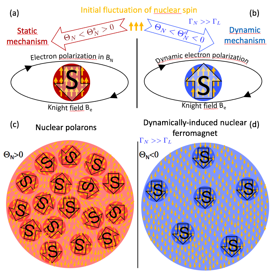
Figure 1: Two kinds of magnetic ordering. Left: At positive nuclear spin temperature local magnetic order (polaron) around each localized electron with spin $S$ may form. The electron spin and the nuclear spins are anti-parallel (a). Polaron spins are oriented randomly, there is no long-range ordering (c). Right: At negative nuclear spin temperature electron and nuclear spins are parallel (b). Dynamic polarization of electron spins by the cold NSS may lead to the emergence of the long-range ferromagnetic order (d) if hyperfine mechanism of electron spin relaxation dominates over spin-orbit interaction.

Nuclear magnetism is a special case, because interactions between nuclear spins, either dipolar or mediated by hyperfine interaction, are much weaker than electronic spin interactions. For this reason, critical temperatures for nuclear spin ordering in metals or insulators are generally less than 1 $\mu$K [7], except for Van Vleck paramagnets [8] and solid He³ [9], where they are in the mK range. Nevertheless, since nuclear spin systems (NSSs) offer a reach and original playground in the field of magnetism, they have motivated a large body of research [7, 10, 11, 12, 13, 1, 14, 15, 16, 8, 17, 18, 19]. Because NSS reaches an internal equilibrium within a time $T_{2}$, much shorter than the spin-lattice relaxation time $T_{2}\ll T_{1}$, nuclear spins can be cooled down to temperatures much lower than the lattice temperature [20, 21, 21, 22]. NSSs also offer a unique opportunity to explore the magnetic phase diagram at negative temperatures [23]. In these quite unusual conditions the thermodynamics tells us that the system tends to maximize its free energy, and antiferromagnetic interactions may lead to a ferromagnetic order [12, 7].

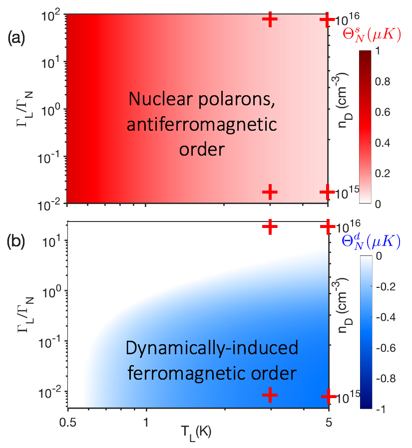
Figure 2: Magnetic phase diagram calculated for n-GaAs NSS cooled down to either positive (a) or negative (b) spin temperature, as a function of the ratio between spin-orbit and hyperfine electron spin relaxation rates $\Gamma_{\text{L}}/\Gamma_{\text{N}}$ and lattice temperature $T_{\text{L}}$. (a) Randomly oriented nuclear polarons may form in the entire parameter space, the critical temperature $\Theta_{\text{N}}^{\text{s}}>0$ is given by Eq. (6). (b) Ferromagnetic order emerges in the parameter space given by Eq. (7), at $\Theta_{\text{N}}^{\text{d}}<0$ given by Eq. (5). Red crosses indicate the points in the parameter space addressed in Figs. 3 and 5. Right scale shows donor densities corresponding to the values of $\Gamma_{\text{L}}/\Gamma_{\text{N}}$ in GaAs.

Most of the experimental work has been performed in metals, better adapted to demagnetization cooling due to their high thermal conductivity [7]. In insulators nuclear spins were first cooled to the milli-Kelvin range by dynamic nuclear polarization using the solid state effect. Final cooling was obtained by adiabatic demagnetization in the rotating frame, to avoid the fast nuclear spin relaxation by paramagnetic impurities which takes place at zero magnetic field [11]. For semiconductors, it was shown theoretically that, similarly to insulators, nuclear magnetic ordering should emerge below a critical temperature [14, 24]. Later, quite different magnetically ordered states have been predicted to form in lightly n-doped semiconductors in the presence of localized electron states. The localized states could be either those of shallow donors in n-doped semiconductors in the insulating regime, or weakly strained quantum dots . It was suggested that hyperfine interaction between a localized electron spin and NSS could give rise to the formation of the anti-ferromagnetic ordering in the vicinity of each donor, see Fig. 1 (a) [1, 18, 19]. Such a state was called nuclear spin polaron, in analogy with the magnetic polaron extensively studied (both theoretically and experimentally) in diluted magnetic semiconductors (DMSs) [26]. In DMSs the polaron consists of a cloud of spins of magnetic impurities (playing the role of nuclei) ordered under the orbit of a localized electron or hole, and the ordering is induced by the exchange interaction (rather than hyperfine interaction). While the formation of magnetic polarons in DMS has been demonstrated in numerous experiments, the implementation of the polaron in NSS is still awaiting its experimental demonstration. In the following the mechanism underlying the formation of this kind of states will be referred to as static mechanism, because it involves electron spin relaxation towards thermodynamic equilibrium with the crystal lattice.

In this paper, we extend and amend the existing theory of magnetically ordered states in n-doped semiconductors. Our model accounts not only for the electron spin relaxation towards its thermal equilibrium with the lattice, but also for eventual dynamic polarization of electrons by the NSS that becomes important when NSS is cooled down to negative temperature . We show that if electron spin relaxation via hyperfine interaction dominates over spin-lattice relaxation, long-range ferromagnetic order should emerge at negative nuclear spin temperature below a critical value. The underlying mechanism will be referred to as dynamic mechanism, since it involves dynamic polarization of the electron spins by the NSS.

Taking into account both static and dynamic mechanisms, we construct the magnetic phase diagram of the coupled electron-nuclei spin system. Its implementation for n-GaAs is shown in Fig. 2. At positive nuclear spin temperature below $\Theta_{\text{N}}^{\text{s}}>0$, the NSS aligns antiferromagnetically with the electron spin due to static mechanism, so that the ensemble of randomly oriented nuclear polarons emerge. $\Theta_{\text{N}}^{\text{s}}$ decreases when lattice temperature increases, but does not depend on the ratio $\Gamma_{\text{L}}/\Gamma_{\text{N}}$, see Fig. 2 (a). At negative nuclear spin temperature below critical $\Theta_{\text{N}}^{\text{d}}<0$ (Fig. 2 (b)) a long-range ferromagnetic order builds up in a wide area of the ($\Gamma_{\text{L}}/\Gamma_{\text{N}}$, $T_{\text{L}}$) parameter space. This type of ordering is controlled by the dynamic mechanism, and has been overseen so far.

The paper is organised in seven sections, including appendix. In the next Section we present a model describing an ensemble of weakly interacting electron spins localised on shallow donors in a bulk semiconductor, or in QDs, each of them being coupled to the underlying nuclei and an external heat bath (crystal lattice). Rate equations describing this system are derived in Appendix. They allow us to introduce the basic phenomenology of the magnetically ordered states and to identify the positive feedback loops that govern their formation. In Section III we go beyond the approximation of homogeneous magnetisation, and account for spatial correlations within NSS. These correlations are critically important, since they determine the nature of the ordered states: the nuclear polarons ensemble is characterized by zero correlation length, while the ferromagnetic order extends over the entire system. Two next Sections (IV and V) address the possibility of the experimental detection of the nuclear spin correlations and ordering. They are followed by concluding remarks.

II Phenomenology of the feedback loop at positive and negative temperatures

Let us consider spin relaxation of an ensemble of localized electrons interacting with NSS cooled down to temperature $\Theta_{\text{N}}<T_{\text{L}}$. Each electron spin interacts with $N$ nuclei. The electron spin correlation time $\tau_{\text{c}}$ is supposed to be short. This means that $\tau_{\text{c}}$ at a given localization center (impurity or QD) is much shorter than the period of the electron spin precession in the Overhauser field $B_{\text{N}}$ created by the random fluctuations of nuclear spin in the vicinity of this center. In this case the relaxation time of the entire electron spin ensemble is longer than $\tau_{\text{c}}$, because electron hopping between centers, as well as the exchange interaction between localized electrons, are nearly spin-conserving. Small spin-orbit corrections to the conduction-band Hamiltonian lead to the relaxation of the ensemble mean spin at rate $\Gamma_{\text{L}}<<1/\tau_{\text{c}}$. The regime of short correlation time is relevant in the majority of experiments on the electron-nuclear spin dynamics in bulk semiconductors and nanostructures, with the exception of single quantum dots [28, 29, 30].

Due to some fluctuation, the average electron spin $\langle\vec{S}\rangle$ (supposed to be homogeneous in space) may differ from zero $\langle\vec{S}\rangle=\langle{S}_{z}\rangle\vec{e_{z}}$. Then, the Knight field $B_{e}$ created by non-zero electron spin gives rise to the nuclear spin polarization and thus the average nuclear spin in the same direction. The dynamics of this ensemble can be described by the following rate equation:

$$\langle\dot{{S}_{z}}\rangle=-\Gamma_{\text{S}}(\langle{S}_{z}\rangle-{S_{\text{T}}})+\Gamma_{\text{N}}\frac{\langle{J}_{z}\rangle}{2\langle{J}_{\perp}^{2}\rangle}\left(1-\frac{\langle{S}_{z}\rangle{S_{\text{T}}}}{S^{2}}\right)$$ (1)

Here $\langle{J}_{\perp}^{2}\rangle$ is the mean squared transverse (perpendicular to the Knight field) fluctuation of the total nuclear spin interacting with the electron, $S=1/2$ is the electron spin value, $S_{\text{T}}$ is the equilibrium value of the electron spin in the presence of the spin-polarized nuclei at a given lattice temperature $T_{\text{L}}$. Derivation of Eq. (1) from the basic laws of quantum mechanics is provided in Sec. VII.1.

In this work we limit our considerations to the case of weak polarization of electron and nuclear spins, which remains relevant until collective electron-nuclei spin states are not formed. In this approximation $\langle{S}_{z}\rangle{S_{\text{T}}}\approx 0$ and $2\langle{J}_{\perp}^{2}\rangle\approx 4I(I+1)/3\equiv Q$. Thus, Eq. (1) reduces to:

$$\langle\dot{{S}_{z}}\rangle=-\Gamma_{\text{S}}(\langle{S}_{z}\rangle-{S_{\text{T}}})+\Gamma_{\text{N}}\frac{\langle{J}_{z}\rangle}{Q}$$ (2)

Its first term on the right-hand side accounts for the relaxation of the electron mean spin towards its value at thermal equilibrium with the lattice, $S_{\text{T}}$, at the rate $\Gamma_{\text{S}}=\Gamma_{\text{L}}+\Gamma_{\text{N}}$. The second term is related to electron-nuclei spin flips. This term was not considered in the nuclear magnetism models developed previously. It allows for the dynamic polarization of the electron by the cold nuclei and is responsible for out-of-equilibrium electron spin polarization. Assuming that the wavefunction of the localised electron has a spherically symmetric exponential form characterised by the Bohr radius $a_{\text{B}}$ we can write the average nuclear spin projection on the Knight field as

$$\langle J_{z}\rangle=-\frac{I(I+1)}{3N}\langle{S}_{z}\rangle\langle{A}\rangle\beta_{\text{N}}.$$ (3)

Here $I$ is the nuclear spin value (assumed to be identical for all nuclear species in the crystal), $\beta_{\text{N}}$ is the inverse nuclear spin temperature expressed in energy units, $\beta_{\text{N}}=1/k_{\text{B}}\Theta_{\text{N}}$, $k_{\text{B}}$ is the Boltzmann constant, $\langle A\rangle=\sum_{l}{\mathcal{A}_{l}A_{l}}$ is the hyperfine interaction constant averaged over all nuclear species in the crystal, $A_{l}$ and $\mathcal{A}_{l}$ are the hyperfine constant and the abundance of $l$-th isotope, respectively, $N=27\pi a_{\text{B}}^{3}/8v_{0}$ is the number of nuclei under the donor orbit, $v_{0}$ is the volume of the crystal elementary cell. Within the same approximation the electron spin polarization at equilibrium, $S_{\text{T}}$, reads:

$$S_{\text{T}}=-\frac{\langle{A}\rangle\beta_{\text{L}}}{4}\kappa\langle{J}_{z}\rangle,$$ (4)

where $\beta_{\text{L}}=1/k_{\text{B}}T_{\text{L}}$ is the inverse lattice temperature expressed in energy units, $\kappa=27n_{0}/64$ and $n_{0}$ is the number of atoms in the crystal elementary cell.

Equation (2), with $\langle J_{z}\rangle$ and $S_{\text{T}}$ given by Eqs. (3) and (4), may have non-trivial static solutions. The static solution of Eq. (2) $\langle\vec{J}\rangle=\langle\vec{S}\rangle=0$ becomes unstable at some critical value of the nuclear spin temperature

$$k_{\text{B}}\Theta_{\text{N}}^{\text{c}}=\frac{Q\kappa\langle A\rangle^{2}\beta_{\text{L}}}{16N}-\frac{\langle A\rangle}{4N}\frac{\Gamma_{\text{N}}}{\Gamma_{\text{S}}},$$ (5)

In the case $\langle A\rangle<0$, $\Theta_{\text{N}}^{\text{c}}$ is always positive. The static and dynamic mechanisms are both acting in concert to achieve a collective nuclear spin state. Whereas if $\langle A\rangle>0$, $\Theta_{\text{N}}^{\text{c}}$ can be either positive or negative depending on both lattice temperature and the ratio $\Gamma_{\text{N}}/\Gamma_{\text{L}}$.

In the limit where dynamic polarisation of electrons by the cold NSS can be neglected (the second term in Eq. (2) is close to zero if $\Gamma_{\text{N}}\ll 1$) Eq. (5) yields the positive value of the critical temperature

$$k_{\text{B}}\Theta_{\text{N}}^{\text{s}}=\frac{Q\kappa\langle A\rangle^{2}\beta_{\text{L}}}{16N}$$ (6)

corresponding to the formation of the polaron state via static mechanism only, as first described by I. Merkulov [1].

The formation mechanism of the ordered state at positive nuclear spin temperature is similar to that of the polaron predicted by I. Merkulov, or the magnetic polaron in DMSs [26]. It can be understood in terms of effective fields, the nuclear (Overhauser) field acting on the electron spin and the electron (Knight) field $B_{e}$ acting on the nuclei. Let us suppose that the electron spin gets polarized to its thermal equilibrium value in a fluctuation of the nuclear field. The Knight field created by such polarized electron acts on the nuclear spins, enhancing the initial fluctuation. This closes the feedback loop and, if the gain is larger than one, the initial fluctuation will grow until a nuclear polaron is formed. If, like in GaAs, the hyperfine coupling constant $\langle A\rangle$ is positive, the electron polarization is anti-parallel to the nuclear spins. We would like to point out that directions of net spins of different static polarons need not be correlated, because the electron spin at each site tends to relax to its equilibrium value in the local Overhauser field.

However, the formation of randomly oriented polarons cannot be consistently described by Eq. (5) obtained assuming homogeneous average spin polarization. Thus, one should go beyond this approximation and consider spatial correlations between nuclear spins at different electron sites. This is done in the next Section, where we show that at $\Theta_{\text{N}}>0$ the magnetic ordering occurs in the form of randomly oriented nuclear polarons even in presence of dynamic polarization (i.e. at nonzero $\Gamma_{\text{N}}$). The instability arises at $\Theta_{\text{N}}$ equal to $\Theta_{\text{N}}^{\text{s}}>0$ given by Eq. (6), see Fig. 2 (a).

The mechanism responsible for magnetic ordering at negative spin temperature is efficient if the electron spin is loosely coupled to the lattice, so that the static mechanism of electron polarisation is overcome by the dynamic one in Eq. (1). In this case the electron spin polarization is always parallel to that of nuclear spins, in contrast with the static polaron case. At negative $\Theta_{\text{N}}$ this provides the positive feedback loop (Fig. 1 (b, d)). The ferromagnetic alignment of the NSS and electrons builds up below the critical temperature given by Eq. (5), provided that the ratio $\Gamma_{\text{N}}/\Gamma_{\text{L}}$ is big enough. Thus, the conditions for the ferromagnetic ordering read:

$$k_{\text{B}}\Theta_{\text{N}}^{\text{d}}=\frac{Q\kappa\langle A\rangle^{2}\beta_{\text{L}}}{16N}-\frac{\langle A\rangle}{4N}\frac{\Gamma_{\text{N}}}{\Gamma\text{S}},$$

$$\frac{\Gamma_{\text{L}}}{\Gamma_{\text{N}}}<\frac{4}{Q\kappa\langle A\rangle\beta_{\text{L}}}-1,$$ (7)

In contrast to the static mechanism, the dynamic mechanism involves the onset of the net spin polarization in the ensemble of electrons, since in the regime of short correlation time the non-equilibrium electron spin is spread over a large number of localization centers. We will show in the next Section that this kind of magnetic order expands over the entire system, so that the resulting long-range state can be qualified as a carrier-induced nuclear ferromagnet (Fig. 2 (b)).

The above considerations allow us to make some predictions about magnetic ordering as a function of the nuclear spin temperature $\Theta_{\text{N}}$, lattice temperature $T_{\text{L}}$ and electron spin correlation time $\tau_{\text{c}}$ that governs the ratio $\Gamma_{\text{N}}/\Gamma_{\text{L}}$. However, in order to quantify the spatial extension of these states (which, as it was anticipated depends on the sign of the nuclear spin temperature) one should address the spatial dependence of the NSS susceptibility. [28, 31]. This is the subject of the next Section.

III Spatial dependence of the electron-induced nuclear magnetization: randomly oriented polarons versus nuclear ferromagnet

The mean spin of electrons as function of time and spatial coordinates (on the spatial scale much greater than average distance between donors) obeys the continuity equation:

$$\langle\dot{{S_{z}}}(\vec{R_{n}})\rangle=-\Gamma_{\text{S}}(\langle{S_{z}}(\vec{R_{n}})\rangle-S_{\text{T}}(\vec{R_{n}}))+\frac{\Gamma_{\text{N}}\langle{J_{z}}(\vec{R_{n}})\rangle}{Q}+\\ \mathrm{div}\left[D_{\text{s}}\nabla(\langle{S_{z}}(\vec{R_{n}})\rangle-S_{\text{T}}(\vec{R_{n}}))\right],$$ (8)

were $\vec{R_{i}}$ defines the n-th donor coordinate in space, while $\langle{S_{z}}(\vec{R_{n}})\rangle$, ${S_{\text{T}}}(\vec{R_{n}})$ stand for mean and equilibrium values of the electron spin projections at n-th donor, respectively and $\langle{J_{z}}(\vec{R_{n}})\rangle$ is the mean nuclear spin at n-th donor, see Eqs. (3)-(4). Eq. (8) is analogous to Eq. (2), but includes an additional term. It accounts for the electron spin diffusion between donors, which is characterized by the diffusion constant $D_{\text{s}}$.

In Fourier components Eq. (8) reads:

$$i\omega\langle{S_{z}}\rangle_{\omega,\vec{k}}=-\Gamma_{\text{S}}{\Upsilon}+\Gamma_{\text{N}}\frac{\langle{J_{z}}\rangle_{\omega,\vec{k}}}{Q}-D_{\text{s}}k^{2}{\Upsilon},$$ (9)

where, $\vec{\Upsilon}=\langle\vec{S}\rangle_{\omega,\vec{k}}+\kappa\langle A\rangle\beta_{\text{L}}\langle\vec{J}\rangle_{\omega,\vec{k}}/4$ and

$$\langle{J_{z}}\rangle_{\omega,\vec{k}}=N_{\text{D}}^{-1}\sum_{n}\langle{J_{z}}(\vec{R}_{n})\rangle_{\omega}\exp(i\vec{k}\cdot\vec{R}_{i}),$$ (10)

$$\langle{S_{z}}\rangle_{\omega,\vec{k}}=N_{\text{D}}^{-1}\sum_{n}\langle{S_{z}}(\vec{R}_{n})\rangle_{\omega}\exp(i\vec{k}\cdot\vec{R}_{n}),$$ (11)

where $N_{\text{D}}$ is the number of donors in the sample, and we assume that $k<<n_{\text{D}}^{1/3}$, $n_{\text{D}}$ being the concentration of the donors. Since the number of nuclei interacting with one electron, $N$, is large, and electron spin dynamics is much faster than that of nuclei, the effect of electron-nuclear interaction on the nuclear spin susceptibility $\chi(\omega,\vec{k}$) can be considered in the mean-field approximation. This way, the Fourier components of nuclear and electron spin at the n-th donor are related via

$$\langle{{J_{z}}(\vec{R}_{n})}\rangle_{\omega}=\frac{\chi(\omega)}{Nn_{\text{D}}}\left(b_{1}\exp(i\vec{k}\cdot\vec{R}_{n})+\overline{b}_{e}\langle{S_{z}}(\vec{R}_{n})\rangle_{\omega}\right),$$ (12)

where $\overline{b}_{e}=-\langle A\rangle/(N\hbar\langle\gamma_{\text{N}}\rangle)$ is the Knight field at saturation, $b_{1}$ is an arbitrary oscillating field parallel to it, $\gamma_{\text{N}}$ is the nuclear gyromagnetic ratio averaged over the nuclear species in the crystal, and $\hbar$ is the reduced Plank constant.

Since we are interested in the “nuclear” scale of frequencies, the condition $\omega/\Gamma_{\text{S}}<<1$ is always fulfilled, and we can put the left-hand side of Eq. (9) equal to zero. Then, from Eqs. (9) and (12) we obtain:

$$\langle{S_{z}}\rangle_{\omega,\vec{k}}=\langle{J_{z}}\rangle_{\omega,\vec{k}}\zeta(\vec{k})$$ (13)

$$\langle{J_{z}}\rangle_{\omega,\vec{k}}=\frac{1}{Nn_{\text{D}}}\frac{\chi(\omega)}{1-\zeta(\vec{k})\overline{b}_{e}\chi(\omega)/(Nn_{\text{D}})}{b}_{1},$$ (14)

where

$$\zeta(\vec{k})=-\frac{\langle A\rangle\kappa\beta_{\text{L}}}{4}+\frac{\Gamma_{\text{N}}}{Q(\Gamma_{\text{S}}+D_{\text{s}}{|\vec{k}|}^{2})}.$$ (15)

Eq. (14) allows one to calculate the $\vec{k}$-dependence of the total fluctuation power $\langle J_{z}^{2}\rangle_{0,\vec{k}}$, as well as the total static susceptibility of the nuclear spin $\chi_{0,\vec{k}}$:

$$\langle J_{z}^{2}\rangle_{0,\vec{k}}=\frac{Q/4}{1+\zeta(\vec{k})\langle A\rangle\beta_{\text{N}}Q/4N}$$ (16)

$${\chi}_{0,\vec{k}}=Nn_{\text{D}}\hbar\langle\gamma_{\text{N}}\rangle\langle J_{z}^{2}\rangle_{0,\vec{k}}$$ (17)

The divergence of the susceptibility is a signature of the collective state formation. The spatial correlation function of the nuclear spin fluctuations is given by the Fourier image $\mathcal{F}(r)$ of Eq. (16). It contains all the information on the spatial ordering of the nuclear spin, including its correlation length $r_{\text{c}}$.

$$\mathcal{F}(r)=\frac{\delta(r)}{1-\beta_{\text{N}}/\beta_{\text{N}}^{s}}-\frac{\langle A\rangle\Gamma_{\text{N}}}{4ND_{\text{s}}}\times\frac{\beta_{\text{N}}}{(1-\beta_{\text{N}}/\beta_{\text{N}}^{\text{s}})^{2}}\times\frac{e^{-r/r_{\text{c}}}}{4\pi r},$$ (18)

with

$$r_{\text{s}}=\sqrt{\frac{D_{\text{s}}}{\Gamma_{\text{S}}}\times\frac{1-\beta_{\text{N}}/\beta_{\text{N}}^{\text{s}}}{1-\beta_{\text{N}}/\beta_{\text{N}}^{\text{d}}}}$$ (19)

where we defined the inverse critical temperatures as $\beta_{\text{N}}^{\text{d}}=1/(k_{\text{B}}\Theta_{\text{N}}^{\text{d}})$ and $\beta_{\text{N}}^{\text{s}}=1/(k_{\text{B}}\Theta_{\text{N}}^{\text{s}}$). The first term in Eq. (18) corresponds to the absence of any correlations between nuclear spins situated under the orbits of two different donors, while the second gives the contribution of carrier-induced magnetic ordering on the scale of $r_{\text{c}}$.

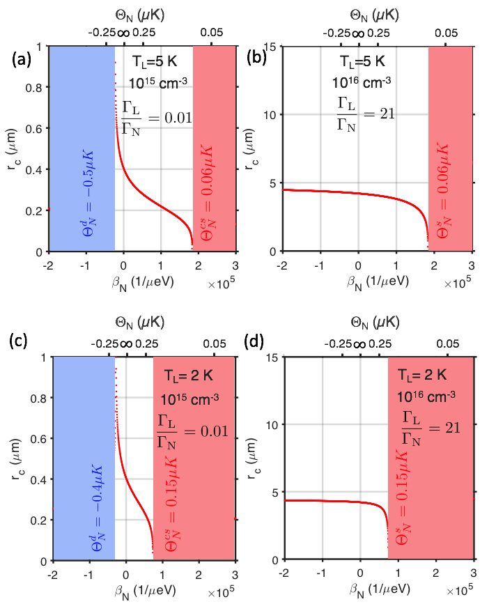
Figure 3: Correlation length $r_{\text{c}}$ calculated using Eq. (19) as a function of nuclear spin temperature $\Theta_{\text{B}}$ (upper scale) or inverse nuclear spin temperature $\beta_{\text{N}}$ (lower scale). Two values of the lattice temperature $T_{\text{L}}=5$ K (a, b), $T_{\text{L}}=2$ K (c,d) and two different donor densities $n_{\text{D}}=10^{15}$ cm^-3 (a, c), $n_{\text{D}}=10^{16}$ cm^-3 (b, d) are shown.

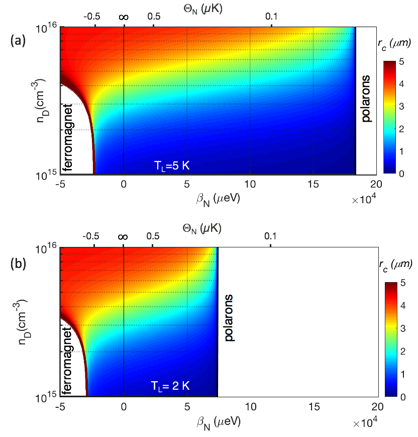
Figure 4: Color-encoded correlation length $r_{\text{c}}$ calculated for n-GaAs using Eq. (19) at $T_{\text{L}}=5$ K (a) and $T_{\text{L}}=2$ K (b) as a function of donor density and nuclear spin temperature.

It is easy to see that both the correlation length $r_{\text{c}}$, and the static susceptibility to uniform magnetic fields, $\chi_{0,\vec{k}=0}$, diverge at negative critical temperature $\Theta_{\text{N}}^{\text{d}}$, where ferromagnetic ordering is expected due to dynamic feedback mechanism. Thus, because at $\Theta_{\text{N}}^{\text{d}}$ the correlation length $r_{\text{c}}\rightarrow\infty$, the dynamic mechanism leads to the formation of a long-range ferromagnetic order, as sketched in Fig. 1 (d).

At $\Theta_{\text{N}}^{\text{s}}>0$ given by Eq. (6), where static mechanism dominates over the dynamic one, and the electron spin aligns anti-ferromagnetically with nuclei, the correlation function $\mathcal{F}(r)$ diverges, while the correlation length goes to zero, $r_{\text{c}}\rightarrow 0$. This means that local nuclear spin fluctuations grow in amplitude, remaining spatially uncorrelated. Eventually, these fluctuations develop into magnetic polarons. Thus, static mechanism of electron-nuclei interaction leads to the formation of the individual polaron states with random spin orientation sketched in Fig. 1 (d). Remarkably, the values of corresponding critical temperature $\Theta_{\text{N}}^{\text{s}}$ given by Eq. (6) are those that one would obtain by simply neglecting the dynamic polarization term in Eq. (2) [1, 18, 19]. This means that dynamic polarization does not alter the formation of the individual randomly oriented polarons. The reason for this is that in the ensemble of randomly oriented polarons the net nuclear spin is zero, and no directional transfer of angular momentum into the electron spin system occurs.

The values of positive and negative critical temperature obtained in this framework are color-encoded in Figs. 2 (a,b) as a function of lattice temperature and $\Gamma_{\text{L}}/\Gamma_{\text{N}}$. These magnetic phase diagrams represent the main result of this paper.

Using the parameters of the NSS in n-GaAs (summarized in Appendix VII.2) we represent in Fig. 3 the critical length $r_{\text{c}}$ calculated for two values of the lattice temperature and two donor densities (the corresponding points of the parameter space are indicated by red crosses in Fig. 2). One can see that the correlation length varies monotonously as a function of the inverse nuclear spin temperature: from infinity at $\Theta_{\text{N}}^{\text{d}}<0$ where ferromagnetic order is expected, to zero at $\Theta_{\text{N}}^{\text{s}}>0$ where nuclear polarons emerge. If the parameters of the system are such that the ferromagnetic order can never emerge (white area in Fig. 2 (b), the correlation length does not diverge at negative temperature. This is illustrated in Fig. 3 (d)).

In the limit of high nuclear spin temperature ($\beta_{\text{N}}\rightarrow 0$) the correlation length is given by $r_{\text{c}}^{\infty}=\sqrt{D_{\text{s}}/\Gamma_{\text{S}}}$. It is governed by the interplay between electron spin flip and diffusion efficiency. $r_{\text{c}}^{\infty}$ depends on the donor concentration (see Fig. 4) and can be interpreted as a spin diffusion length.

Note also, that regardless the type of magnetic ordering, the correlation length varies strongly in the vicinity of the ordering transition. This is illustrated in Fig. 4. It shows the correlation length as function of nuclear spin temperature and donor density at $T_{\text{L}}=5$ K (a) and $T_{\text{L}}=2$ K (b). The parameters of the calculation are given in Appendix VII.2 ). On can see that the variation of the critical length with nuclear spin temperature can reach several micrometers. This suggests that even above the critical temperature these correlations may be detected, e.g via spin noise spectroscopy. This possibility is analysed in the next Session.

IV Sensing nuclear spin correlations and ordering by spin noise spectroscopy

One of the promising methods that can be used to evidence electron-induced nuclear spin ordering is the electron spin-noise spectroscopy (SNS) [32, 33, 34, 35]. SNS is based on the fluctuation-dissipation theorem, which states that it is possible to detect resonances of linear susceptibility by “listening“ to a noise of the medium in its equilibrium state. It allows one to probe electron spin fluctuations non-perturbatively using absorption-free Faraday rotation. The Faraday rotation noise spectrum features a peak at the magnetic resonance frequency $\nu_{\text{L}}$ corresponding to precession of spontaneous fluctuations of the spin ensemble at the Larmor frequency. The latter is given by the total magnetic field acting on the electron, that is a sum of the external field and the Overhauser field $B_{\text{N}}$ [36]. Thus, one can expect that the formation of the ordered state at $B=0$ will be accompanied by the shift of the electron spin-noise spectrum peak from zero to $\gamma_{e}B_{\text{N}}$, where $\gamma_{e}$ is the electron gyromagnetic ratio.

Even above the critical temperature, the correlations induced by the electrons in the deeply cooled nuclear spin system can be detected via SNS. One could detect variations of the correlation length in the electron spin fluctuations in the vicinity of the critical temperature by the recently developed spatiotemporal spin noise spectroscopy [35]. Another possibility would be to detect directly the nuclear spin noise [37]. Below we study how the correlations in the NSS affect the shape of the electron spin noise spectrum.

The spectral power density $\langle S_{z}^{2}(\omega)\rangle$ of electron spin fluctuations can be expressed in terms of the total nuclear spin fluctuation power$\langle J_{z}^{2}\rangle_{0,\vec{k}}$ given by Eq. (16), normalized by the square of the total spin value $\overline{\langle J_{z}^{2}\rangle_{0,\vec{k}}}=3\langle J^{2}\rangle_{0,\vec{k}}/I(I+1)$:

$$\langle S_{z}^{2}(\omega)\rangle=\left[\left(\frac{\Omega_{\text{N}}^{2}}{3\pi^{2}n_{\text{D}}}\int_{0}^{k^{\prime}}\frac{D_{\text{s}}k^{4}\times\overline{\langle J_{z}^{2}\rangle_{0,\vec{k}}}}{(D_{\text{s}}k^{2})^{2}+\omega^{2}}dk\right)^{2}+\right.\\ \left.+\left(\omega-\frac{\Omega_{\text{N}}^{2}}{3\pi^{2}n_{\text{D}}}\int_{0}^{k^{\prime}}\frac{\omega\times\overline{\langle J_{z}^{2}\rangle_{0,\vec{k}}}}{(D_{\text{s}}k^{2})^{2}+\omega^{2}}dk\right)^{2}\right]^{-1},$$ (20)

where $k^{\prime}=2/3\pi^{2}{n_{\text{D}}^{-1/3}\Gamma_{\text{S}}}/\Gamma_{\text{N}}$. The derivation of this expression is given in Appendix VII.3.

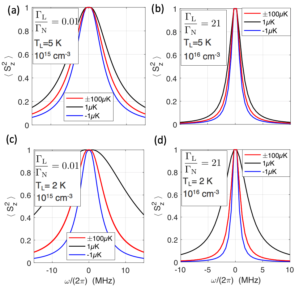
Figure 5: Electron spin noise spectra calculated using Eq. 20 at four different values of the nuclear spin temperature: $\Theta_{\text{N}}=\pm 100$ $\mu$K (these two spectra are almost identical) and $\Theta_{\text{N}}=\pm 1$ $\mu$K. Two values of the lattice temperature $T_{\text{L}}=5$ K (a,b), $T_{\text{L}}=2$ K (c,d) and two different donor densities $n_{\text{D}}=10^{15}$ cm^-3 (a, c), $n_{\text{D}}=10^{16}$ cm^-3 (b, d) are shown.

Fig. 5 shows electron spin noise spectra calculated in n-GaAs for the same combinations of doping and lattice temperature (shown by red crosses in Fig. 2) as the correlation length in Fig. 3. The parameters are given in Appendix VII.2. We compare four values of the nuclear spin temperature: $\Theta_{\text{N}}\pm=100$ $\mu$K and $\Theta_{\text{N}}=\pm 1$ $\mu$K.

The two spectra at $\Theta_{\text{N}}\pm=100$ $\mu$K are almost identical. Indeed, when nuclear spin correlations are negligibly small, then the SN spectrum is just a Lorentzian function with the spectral width at half maximum inversely proportional to the electron spin relaxation time $\textrm{HWHM}=\Gamma_{\text{S}}/2\pi$. The latter does not depend on the sign of the nuclear spin temperature in the absence of correlations, and is determined by the donor density (see Fig. 6.

By contrast, at $\Theta_{\text{N}}=\pm 1$ $\mu$K, when nuclear spin system is cold, but still above the transition temperature, the correlations build up. They affect electron spin relaxation time in a way that depends on the sign of the nuclear spin temperature. At $\Theta_{\text{N}}>0$ electron spin relaxation time shortens. This is the consequence of the reduction of the correlation length in the vicinity of the polaron transition, making motional narrowing inefficient. At $\Theta_{\text{N}}<0$ electron spin relaxation time grows up due to motional narrowing that accompanies the increase of the correlation length. Thus, the onset of correlations can be detected by measuring electron spin noise even above critical temperature.

V Perspectives for experimental observation of the nuclear magnetic ordering.

The potential experimental detection of the electron-induced nuclear correlations and ordering rely on our ability to efficiently cool the NSS. In order to be as realistic as possible, we focus on n-GaAs, where both electron and nuclear spin dynamics have been extensively explored.

In n-doped GaAs ($n_{\text{D}}=2\times 10^{15}$ cm^-3) nuclear spin temperatures as low as $\Theta_{\text{N}}\approx\-2$ $\mu$K have been reported at $T_{\text{L}}\approx 4$ K. This is encouraging, since this value is close to the critical temperature required to reach the ferromagnetic order ($\Theta_{\text{N}}^{\text{d}}\approx-0.5$ $\mu$K).

The method usually employed for deep cooling of the nuclear spin consists of two steps: (i) optical pumping that is mediated by the hyperfine interaction with spin-polarized electrons. Under a magnetic field $B_{i}=200$ G the achieved nuclear spin polarization defines an initial temperature $\Theta_{\text{N}i}$, (ii) adiabatic demagnetization to zero field, that provides further cooling down to $\Theta_{\text{N}}=\Theta_{\text{N}i}B_{\text{L}}/B_{i}$. The effective local field $B_{\text{L}}$ determines the actual efficiency of the cooling. It includes contributions from the dipole-dipole interaction ($B_{\text{dd}}\approx 2$ G) and the quadrupole interaction that can be induced by strain.

Keeping lattice temperature at $T_{\text{L}}\approx 4-5$ K, the optimisation of pumping efficiency, in particular using higher pumping field $B_{i}$ and reducing the strain in the sample, may be sufficient to reach negative temperatures well below the critical value required for the formation of the nuclear ferromagnet in the sample with $n_{\text{D}}\approx 10^{15}$ cm^-3 (see Fig. 2). Eventually, choosing the samples with lower donor densities may increase the absolute value of the critical temperature and favor the formation of the nuclear ferromagnet, but we do not yet have enough data on the electron spin relaxation rates in such low-doped n-GaAs samples. By contrast, most straightforward way of reaching positive critical temperature for the formation of nuclear polarons is to cool the crystal lattice in the sample with $n_{\text{D}}=10^{16}$ cm^-3 (see Fig. 2) well below $T_{\text{L}}=2$ K.

VI Conclusions

We have shown that in n-doped semiconductors with positive hyperfine constant, two kinds of magnetically ordered states can be induced by resident electrons in the deeply cooled nuclear spin system. The magnetic phase diagram is determined by three parameters: lattice temperature, donor density and the sign of the nuclear spin temperature $\Theta_{\text{N}}$.

When NSS is cooled down to a positive temperature below critical one $\Theta_{\text{N}}^{\text{s}}>0$, randomly oriented nuclear spin polarons form under the orbit of each donor. The underlying mechanism relies on the positive feedback, mediated by static polarization of nuclear and electron spins by Knight and Overhauser fields respectively. The critical nuclear spin temperature for the formation of randomly oriented polarons state decreases when the lattice temperature is increased. The models of nuclear polarons have been developed previously, but they neglected dynamic polarisation of the electron spin by the cold NSS. We have shown that the formation of the nuclear polarons is not impeded by dynamic polarisation even when hyperfine relaxation dominates over spin-orbit mechanism.

In NSS cooled down to a negative temperature below critical one $\Theta_{\text{N}}^{\text{d}}<0$, we predict the formation of an original long-range ordered state, that we call dynamically-induced nuclear ferromagnet. It should manifest itself when electron spin dynamics is dominated by the hyperfine coupling, rather than by the spin-orbit interaction. The underlying feedback mechanism can be understood as a dynamic polarization of the localized electron spin by the cold NSS polarized in the Knight field. The dominance of the hyperfine coupling in low-doped systems and QDs is well known and confirmed by numerous experiments, but the positive feedback loop that leads in this case to the nuclear ferromagnetic state has been overseen soo far.

The lifetime of the ordered states is limited by the inevitable heating of the system, on the scale of the order of several seconds in n-GaAs. Within this time, after cooling the NSS to a sufficiently low nuclear spin temperature, the nuclear spin ordering can be detected by different techniques: off-resonant Faraday rotation, spin noise spectroscopy, photoluminescence combined with radio-frequency absorption.

The strategy to reach magnetically ordered states may include lowering down the sample temperature down to and below $2$ K rather than $4-5$ K used in previous experiments, and cooling the NSS at higher magnetic fields prior to adiabatic demagnetization. Finally, samples with unstrained QDs may be promising. Stronger electron localization as compared to donor-bound electrons in bulk n-GaAs ensures stronger interaction between electron and nuclear spins. This may offer higher critical temperatures for both nuclear polarons and dynamically induced-induced nuclear ferromagnetism.

VII Appendix

VII.1 Derivation of the rate equations for the coupled electron-nuclei spin system

The populations of electron spin $S=1/2$ with projections $\pm 1/2$ on the $z$ axis chosen along the Overhauser field are equal to $S\pm\langle S_{z}\rangle$, respectively. The rate equation for the average electron spin projection $\langle S_{z}\rangle$ reads:

$$\langle\dot{S}_{z}\rangle=-\langle{S}_{z}\rangle(p_{+}+p_{-})+S(p_{+}-p_{-}),$$ (A1)

where $p_{+}$ and $p_{-}$ are probabilities of transitions with rising and lowering the electron spin projection by one, correspondingly. Such transitions occur with simultaneous change of states of the nuclear spin system and the lattice: the angular momentum is transferred to nuclei, while the energy goes to the lattice. In fact, these are transitions in the coupled electron-nuclear spin system, induced by interaction with the lattice. As shown in [13] (Ch 8), in the approximation of short correlation time the probabilities of such transitions with mutual electron-nuclear spin flips can be written as:

$$p_{\downarrow m}^{i}=F_{-}\frac{\left(A_{i}v_{0}\Psi_{i}^{2}\right)^{2}\tau_{\text{c}}}{\hbar^{2}}\lvert\langle(m_{i}+1,-S)\lvert\hat{S}_{-}\hat{I}_{+}\rvert(m_{i},S)\rangle\rvert^{2}$$

$$p_{\uparrow m}^{i}=F_{+}\frac{\left(A_{i}v_{0}\Psi_{i}^{2}\right)^{2}\tau_{\text{c}}}{\hbar^{2}}\lvert\langle(m_{i}-1,S)\lvert\hat{S}_{+}\hat{I}_{-}\rvert(m_{i},-S)\rangle\rvert^{2}.$$ (A2)

Here $\hat{I}_{\pm}$ are the rising and lowering nuclear spin operators, $m_{i}$ is the spin projection of the i-th nuclear spin, $\Psi_{i}$ is the absolute value of the electron wave function at the i-th nuclei position, $v_{0}$ is the volume of the crystal elementary cell, $A_{i}$ is the hyperfine constant of the i-th nucleus and $F_{\pm}$ characterise the spectral power density of a random force describing interaction of the spin system with the lattice. As follows from the principle of detailed balance, $F_{+}/F_{-}=\exp(-\hbar\Omega_{\text{N}}\beta_{\text{L}})$, where $\hbar\Omega_{\text{N}}$ is electron spin splitting in the Overhauser field created by the underlying nuclei. Taking into account that

$$\lvert\langle m_{i}-1\lvert\hat{I}_{-}\rvert m_{i}\rangle\rvert^{2}=\langle m_{i}\lvert\hat{I}_{+}\hat{I}_{-}\rvert m_{i}\rangle=\langle m_{i}\lvert\hat{I}^{2}-\hat{I}_{z}^{2}+\hat{I}_{z}\rvert m_{i}\rangle$$

$$\lvert\langle m_{i}+1\lvert\hat{I}_{+}\rvert m_{i}\rangle\rvert^{2}=\langle m_{i}\lvert\hat{I}_{-}\hat{I}_{+}\rvert m_{i}\rangle=\langle m_{i}\lvert\hat{I}^{2}-\hat{I}_{z}^{2}-\hat{I}_{z}\rvert m_{i}\rangle$$

$$\langle-S\lvert\hat{S}_{+}\rvert S\rangle=\langle S\lvert\hat{S}_{-}\rvert-S\rangle=1$$ (A3)

and averaging over all the projections of each nuclear spin, $m_{i}$, with the distribution function $\rho_{m}$ corresponding to the spin temperature of the nuclear system we obtain the probabilities of the electron spin flip transitions due to interaction with i-th nucleus as

$$p_{-}^{i}=F_{-}\frac{\left(A_{i}v_{0}\Psi_{i}^{2}\right)^{2}\tau_{\text{c}}}{\hbar^{2}}\left[I(I+1)-\langle I_{iz}^{2}\rangle-\langle I_{iz}\rangle\right]$$

$$p_{+}^{i}=F_{+}\frac{\left(A_{i}v_{0}\Psi_{i}^{2}\right)^{2}\tau_{\text{c}}}{\hbar^{2}}\left[I(I+1)-\langle I_{iz}^{2}\rangle-\langle I_{iz}\rangle\right],$$ (A4)

where

$$\langle I_{iz}\rangle=\frac{\sum_{m_{i}=-I}^{I}m_{i}\times\mathrm{exp}(-m_{i}\langle S_{z}\rangle A_{i}v_{0}\Psi_{i}^{2}\beta_{\text{N}})}{\sum_{m_{i}=-I}^{I}\mathrm{exp}(-m_{i}\langle S_{z}\rangle A_{i}v_{0}\Psi_{i}^{2}\beta_{\text{N}})}$$ (A5)

is the average spin projection of the i-th nucleus on the z-axis (along Knight and Overhauser fields) and

$$\langle I_{iz}^{2}\rangle=\frac{\sum_{m_{i}=-I}^{I}m_{i}^{2}\times\mathrm{exp}(-m_{i}\langle S_{z}\rangle A_{i}v_{0}\Psi_{i}^{2}\beta_{\text{N}})}{\sum_{m_{i}=-I}^{I}\mathrm{exp}(-m_{i}\langle S_{z}\rangle A_{i}v_{0}\Psi_{i}^{2}\beta_{\text{N}})}$$ (A6)

is the mean squared value of the same projection. In order to obtain the full probabilities of flipping the electron spin up or down, one has to sum Eq. A2 over all the nuclei situated under the orbit of a given electron:

$$p_{-}=(v_{0}\langle A\rangle)^{2}F_{-}\sum_{i}\frac{\Psi_{i}^{4}\tau_{\text{c}}}{\hbar^{2}}\left[I(I+1)-\langle I_{iz}^{2}\rangle-\langle I_{iz}\rangle\right]$$

$$p_{+}=(v_{0}\langle A\rangle)^{2}F_{+}\sum_{i}\frac{\Psi_{i}^{4}\tau_{\text{c}}}{\hbar^{2}}\left[I(I+1)-\langle I_{iz}^{2}\rangle+\langle I_{iz}\rangle\right],$$ (A7)

where $\langle A\rangle=\sum_{l}{\mathcal{A}_{l}A_{l}}$ is the hyperfine interaction constant averaged over all nuclear species in the crystal, $A_{l}$ and $\mathcal{A}_{l}$ are the hyperfine constant and the abundance of $l$-th isotope, respectively. We can now define electron spin relaxation rate due to hyperfine interaction as

$$\Gamma_{\text{N}}\equiv(v_{0}\langle A\rangle)^{2}(F_{+}+F_{-})\sum_{i}\frac{\Psi_{i}^{4}\tau_{\text{c}}}{\hbar^{2}}\left[I(I+1)-\langle I_{iz}^{2}\rangle\right],$$ (A8)

the thermal equilibrium value of the mean electron spin $S_{\text{T}}$:

$$2S_{\text{T}}=\frac{F_{+}-F_{-}}{F_{+}+F_{-}},$$ (A9)

mean z-projection of the ensemble of the nuclear spins interacting with a given electron

$$\langle J_{z}\rangle=\frac{\sum_{i}\Psi_{i}^{4}\langle I_{iz}\rangle}{\sum_{i}\Psi_{i}^{4}},$$ (A10)

and mean squared transverse (perpendicular to z-axis) fluctuation of the ensemble of the nuclear spins interacting with a given electron.

$$\langle J_{\perp}^{2}\rangle=I(I+1)-\frac{\sum_{i}\Psi_{i}^{4}\langle I_{iz}^{2}\rangle}{\sum_{i}\Psi_{i}^{4}},$$ (A11)

By substituting Eqs. (A7) into Eq. (A1) and using the above definitions we obtain:

$$\langle\dot{{S}_{z}}\rangle=-\Gamma_{\text{N}}\left(\langle S_{z}\rangle-S_{\text{T}}\right)+\Gamma_{\text{N}}\frac{\langle{J}_{z}\rangle}{2\langle J_{\perp}^{2}\rangle}\left(1-\frac{\langle{S}_{z}\rangle S_{\text{T}}}{S^{2}}\right).$$ (A12)

If, in addition to relaxation by nuclei, there is some spin-orbit relaxation, this equation should be complimented by the term $-\Gamma_{\text{L}}\left(\langle S_{z}\rangle-S_{\text{T}}\right)$ on the right-hand side. In this case the full equation describing both hyperfine and spin-orbit relaxation in the ensemble of localized electrons takes the form given by Eq. (1) in the main test.

As far as collective electron-nuclei spin states are not formed, both electron and nuclear spin polarisation remain weak. Under these conditions $\langle J_{\perp}^{2}\rangle\approx 2I(I+1)/3$ and $\langle S_{z}\rangle S_{\text{T}}\rightarrow 0$. Assuming the exponential form of the electron wavefunction $\Psi_{i}\propto\exp(-r_{i}/a_{\text{B}})$, where $a_{\text{B}}$ is the Bohr radius of the donor-bound electron we can calculate $\langle J_{z}\rangle\approx-I(I+1)\beta_{\text{N}}\langle A\rangle\langle S_{z}\rangle/3N$. Here $N$ is defined as

$$\frac{1}{N}\equiv v_{0}\frac{\sum_{i}\Psi_{i}^{6}}{\sum_{i}\Psi_{i}^{4}}=\frac{8v_{0}}{27\pi a_{\text{B}}^{3}}.$$ (A13)

It can be considered as a number of nuclei under the orbit of donor-bound electron, for shallow donors in GaAs $N\approx 2.4\times 10^{5}$. Thus, Eq. (1) reduces to the linear differential equation:

$$\langle\dot{{S}_{z}}\rangle=-\Gamma_{\text{S}}\left(\langle S_{z}\rangle-S_{\text{T}}\right)+\Gamma_{\text{N}}\frac{\langle{J}_{z}\rangle}{Q},$$ (A14)

with $Q\equiv 4I(I+1)/3$ and

$$S_{\text{T}}=-\frac{1}{2}\textrm{tanh}\left(\frac{\hbar\Omega_{\text{N}}\beta_{\text{L}}}{2}\right)\approx-\frac{\langle A\rangle\langle J_{z}\rangle\kappa\beta_{\text{L}}}{4},$$ (A15)

where $\Omega_{\text{N}}$ is the angular frequency of electron spin precession in root mean square fluctuation of the Overhauser field

$$\hbar\Omega_{\text{N}}=\sqrt{Q\kappa\langle A\rangle^{2}/4N},$$ (A16)

$\kappa=27n_{0}/64$ and $n_{0}$ is the number of atoms in the elementary cell of the crystal. Note, that the factor $\kappa$ appears in Eq. (A15) due to the choice that we have made in the definition of $N$ (cf Eq. (A13)).

VII.2 Parameters of the coupled electron-nuclear spin system in n-GaAs: interaction, diffusion and relaxation

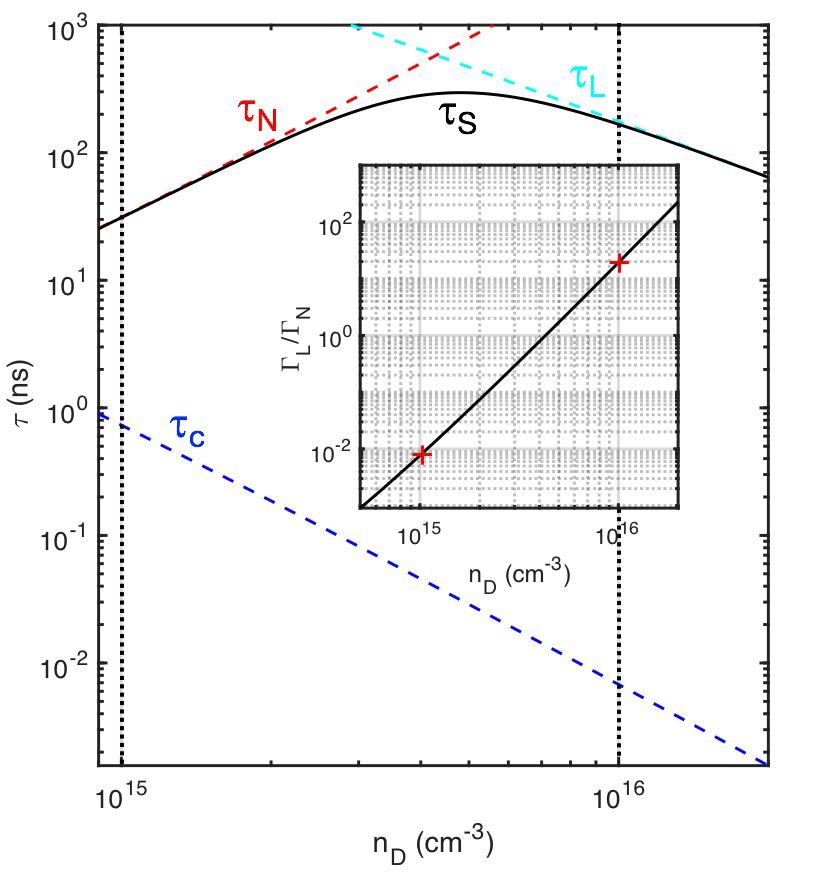
Figure 6: Characteristic times for the electron spin in the insulating n-GaAs as a function of the donor density (dashed lines): correlation time (blue), hyperfine relaxation time (red), spin-orbit relaxation time (cyan). Inset shows the ratio of two relaxation rates as a function of donor density. Vertical dotted lines and red crosses (inset) point the parameters corresponding to Figs. 3 and  5.

Electron spin relaxation has been exhaustively studied in the insulating n-GaAs. Correlation time of the electron spin was measured over a broad range of donor concentrations $n_{\text{D}}$ [29, 30]. Its dependence on $n_{\text{D}}$ can be approximated by the expression:

$$\tau_{\text{c}}(n_{\text{D}})=0.2\left(\frac{n_{\text{D}}}{10^{15}}\right)^{2.3}\text{log}\left(15\frac{n_{\text{D}}}{10^{15}}\right),$$ (A17)

where $n_{\text{D}}$ is expressed in inverse cubic centimetres and $\tau_{\text{c}}$ in nanoseconds.

Electron spin relaxation rate due to hyperfine coupling is given by

$$\Gamma_{\text{N}}=\frac{2}{3}\Omega_{\text{N}}^{2}\tau_{\text{c}},$$ (A18)

where $\Omega_{\text{N}}$ is the angular frequency that characterizes electron spin precession in the fluctuating Overhauser field defined in the previous section, see Eq. A16. The spin-orbit relaxation rate is also related to the correlation time and donor density:

$$\Gamma_{\text{L}}=\frac{n_{\text{D}}^{-2/3}}{L_{\text{SO}}^{2}\tau_{\text{c}}},$$ (A19)

where $L_{\text{SO}}$ is so-called spin-orbit length [28]. In GaAs $L_{\text{SO}}\approx 7$ $\mu$m. Finally, the electron spin diffusion constant, determined by electron hopping and exchange interaction in the impurity band, reads:

$$D_{\text{s}}=\frac{n_{\text{D}}^{-2/3}}{3\tau_{\text{c}}},$$ (A20)

Fig. 6 shows low temperature ($T_{\text{L}}<5$ K) correlation time, as well as two relevant electron spin relaxation times calculated according to Eqs. (A17-A19) as a function of the donor density, while inset shows the ratio $\Gamma_{\text{L}}/\Gamma_{\text{N}}$. The right scale in Fig. 2 shows the donor densities calculated using Eqs. (A17-A19).

Table 1 summarises the values of spin, gyromagnetic ratio, hyperfine constants and abundance for each of the three isotopes in GaAs. Other parameters used in the calculations are listed in Table 2.

parameter	value
Donor Bohr radius, $a_{\text{B}}$	$10$ nm
Volume of the elementary cell, $v_{0}$	$4.5\times 10^{9}$ m-3
Atoms number in the elementary cell, $n_{0}$	$2$
Spin-orbit length, $L_{\text{SO}}$	$7.5$ $\mu$m
Electron gyromagnetic ratio, $\gamma_{e}$	$0.64$ MHz/G

Table 1: Parameters used in numerical calculations for n-GaAs

isotope	${}^{75}As$	${}^{71}Ga$	${}^{69}Ga$
Spin, $I_{l}$	3/2	3/2	3/2
Abundance, $\mathcal{A}_{l}$	0.5	0.2	0.3
Hyperfine constant, $A_{l}$ ($\mu$eV)	43.5	54.8	43.1
Gyromagnetic ratio, $\gamma_{N,l}$ ($10^{7}$rad/Ts)	4.6	8.1	6.44

Table 2: Values of spin, gyromagnetic ratio, hyperfine constants and abundance of each of three isotopes in GaAs [38, 39].

VII.3 Calculation of electron spin noise in the presence of nuclear spin correlations

In order to calculate the spectral power density of electron spin fluctuations in the regime where the fluctuations of nuclear spin can be correlated, we need to develop a method based on $k$-components of the nuclear spin fluctuations. Let us consider a cubic box with the volume $V\gg n_{\text{D}}^{-1}$. Electron and nuclear spin densities in the box can be expanded in the Fourier series with $k_{\sigma,n}=2\pi n/V^{1/3}$, where $\sigma\in\{x,y,z\}$ and $0<n<(Vn_{\text{D}})^{1/3}$. The total number of $k$-modes $Vn_{\text{D}}$ is equal to the number of donors in the volume.

The zero-$k$ mode of the $z$-component of the electron spin density under periodic pump $S_{G}e^{—i\omega t}$ can be written as

$$\dot{S}_{z,0}=\sum_{k}{\Omega_{x,\vec{k}}S_{y,-\vec{k}}}-\sum_{k}{\Omega_{y,\vec{k}}S_{x,-\vec{k}}}+S_{G}e^{i\omega t}$$ (A21)

where $\Omega_{x,\vec{k}}$ and $\Omega_{x,\vec{k}}$ are Fourier components of the nuclear fluctuation field in frequency units. Since the spatial harmonics of $x$ and $y$-components of the electron spin are much smaller than the $z$-component, we keep only the terms containing $S_{z,0}$ in the corresponding equations:

$$\dot{S}_{x,-\vec{k}}=\Omega_{y,-\vec{k}}{S}_{z,0}-D_{\text{s}}k^{2}S_{x,-\vec{k}}$$

$$\dot{S}_{y,-\vec{k}}=-\Omega_{x,-\vec{k}}{S}_{z,0}-D_{\text{s}}k^{2}S_{y,-\vec{k}}$$ (A22)

These equations have the following solutions:

$${S}_{x,-\vec{k}}(t)=\Omega_{y,-\vec{k}}\int_{0}^{\infty}e^{-D_{\text{s}}k^{2}\tau}{S}_{z,0}(t-\tau)\,d\tau$$

$${S}_{y,-\vec{k}}(t)=-\Omega_{x,-\vec{k}}\int_{0}^{\infty}e^{-D_{\text{s}}k^{2}\tau}{S}_{z,0}(t-\tau)\,d\tau$$ (A23)

Substituting Eqs. (A23) into Eq. (A21) we obtain

$$\dot{S}_{z,0}=-\frac{2}{3}\sum_{k}\Omega^{2}_{N,\vec{k}}\int_{0}^{\infty}e^{-D_{\text{s}}k^{2}\tau}{S}_{z,0}(t-\tau)\,d\tau+S_{G}e^{i\omega t},$$ (A24)

where we assumed that nuclear spin fluctuations are isotropic $\frac{2}{3}\Omega^{2}_{N,\vec{k}}=\Omega_{x,\vec{k}}+\Omega_{y,\vec{k}}$. The solution of Eq. (A24) has the form $S_{z,0}(t)=S_{z}(\omega)e^{—i\omega t}$, and we come to the equation for $S_{z}(\omega)$:

$$i\omega{S}_{z}(\omega)=-\Phi(\omega){S}_{z}(\omega)+S_{G}$$ (A25)

with

$$\Phi(\omega)=-\frac{2}{3}\sum_{k}\frac{\Omega^{2}_{N,\vec{k}}}{D_{\text{s}}k^{2}+\omega^{2}}$$ (A26)

Replacing in Eq. (A26) the summation by the integration over $k$-space, we get

$$\Phi(\omega)=\frac{V}{3\pi^{2}}\int_{0}^{\alpha n_{\text{D}}^{1/3}}\frac{k^{2}\Omega_{N,\vec{k}}^{2}(D_{\text{s}}k^{2}-i\omega)}{(D_{\text{s}}k^{2})^{2}+\omega^{2}}dk,$$ (A27)

where the upper integration limit should be determined from the conditions in the absence of correlations: $\Phi(\omega=0)=\Gamma_{\text{S}}$ and $\Omega^{2}_{N,\vec{k}}(\omega=0)=\Omega_{\text{N}}^{2}/Vn_{\text{D}}\equiv\Omega^{2}_{0,\vec{k}}$. Recalling that $D_{\text{s}}$ is given by Eq. (A20), we get

$$\Phi(\omega)=\frac{\Omega_{\text{N}}^{2}}{3\pi^{2}n_{\text{D}}}\int_{0}^{\nu n_{\text{D}}^{1/3}}\frac{k^{2}(\Omega_{N,\vec{k}}^{2}/\Omega_{0,\vec{k}}^{2})(D_{\text{s}}k^{2}-i\omega)}{(D_{\text{s}}k^{2})^{2}+\omega^{2}}dk,$$ (A28)

where $\nu=2/3(\pi^{2}\Gamma_{\text{S}}/\Gamma_{\text{N}})$ and the ratio $\Omega_{N,\vec{k}}^{2}/\Omega_{0,\vec{k}}^{2}$ is nothing but nuclear spin fluctuation power given by Eq. (16), normalized by its maximum value:

$$\Omega_{N,\vec{k}}^{2}/\Omega_{0,\vec{k}}^{2}=3\langle J_{z}^{2}\rangle_{0,\vec{k}}/I(I+1).$$ (A29)

The solution of Eq. (A25) reads:

$${S}_{z}(\omega)=\frac{S_{G}}{i\omega+\Phi(\omega))}$$ (A30)

Now, considering $S_{G}$ as a time harmonic of a $\delta$-correlated random Langevin force, we find the expression for the spectral power density of the electron spin fluctuations:

$$\langle S^{2}_{z}\rangle_{\omega}=\langle S_{z}(\omega)S_{z}(-\omega)\rangle=\\ \frac{{S_{G}}^{2}}{\left(\text{Re}(\Phi(\omega))\right)^{2}+\left(\omega+\text{Im}(\Phi(\omega))\right)^{2}},$$ (A31)

where $\Phi(\omega)$ is given by Eqs. (A28-A29) and $\langle J_{z}^{2}\rangle_{0,\vec{k}}$ by Eq. (16).

References

- Merkulov [1998] I. Merkulov, Formation of a nuclear spin polaron under optical orientation in GaAs-type semiconductors, Physics of the Solid State 40, 930 (1998).
- Stamps et al. [2014] R. L. Stamps, S. Breitkreutz, J. Åkerman, A. V. Chumak, Y. Otani, G. E. W. Bauer, J.-U. Thiele, M. Bowen, S. A. Majetich, M. Kläui, I. L. Prejbeanu, B. Dieny, N. M. Dempsey, and B. Hillebrands, The 2014 Magnetism Roadmap, J. Phys. D. Appl. Phys. 47, 333001 (2014), arXiv:1410.6404 .
- Khomskii [2006] D. I. Khomskii, Multiferroics: Different ways to combine magnetism and ferroelectricity, J. Magn. Magn. Mater. 306, 1 (2006).
- Yazyev and Helm [2007] O. V. Yazyev and L. Helm, Defect-induced magnetism in graphene, Phys. Rev. B 75, 125408 (2007).
- Mroziński [2005] J. Mroziński, New trends of molecular magnetism, Coord. Chem. Rev. 249, 2534 (2005).
- Venkatesan et al. [2004] M. Venkatesan, C. B. Fitzgerald, and J. Coey, Unexpected magnetism in a dielectric oxide, Nature 430, 630 (2004).
- Oja and Lounasmaa [1997] A. S. Oja and O. V. Lounasmaa, Nuclear magnetic ordering in simple metals at positive and negative nanokelvin temperatures, Rev. Mod. Phys. 69, 1 (1997).
- Ishii [2004] H. Ishii, Nuclear Magnetism in Van Vleck Metals, J. Low Temp. Phys. 135, 579 (2004).
- Cross and Fisher [1985] M. C. Cross and S. Fisher, solid SHe: Confrontation, Rev. Mod. Phys. 57, 881 (1985).
- Chapellier et al. [1970] M. Chapellier, M. Goldman, V. H. Chau, and A. Abragam, Production and Observation of a Nuclear Antiferromagnetic State, J. Appl. Phys. 41, 849 (1970).
- Goldman et al. [1974] M. Goldman, M. Chapellier, V. H. Chau, and A. Abragam, Principles of nuclear magnetic ordering, Phys. Rev. B 10, 226 (1974).
- Goldman [1977] M. Goldman, Nuclear dipolar magnetic ordering, Physics Reports 32, 1 (1977).
- Abragam [1961] A. Abragam, The Principles of Nuclear Magnetism (Oxford University Press, Oxford, 1961).
- Merkulov [1982] I. A. Merkulov, Phase transition in the nuclear spin system in a semiconductor with optically oriented electrons, Soviet Physics JETP 55, 188 (1982).
- Juntunen and Tuoriniemi [2005] K. I. Juntunen and J. T. Tuoriniemi, Experiment on Nuclear Ordering and Superconductivity in Lithium, J Low Temp Phys 141, 235 (2005).
- Herrmannsdörfer et al. [1995] T. Herrmannsdörfer, P. Smeibidl, B. Schröder-Smeibidl, and F. Pobell, Spontaneous Nuclear Ferromagnetic Ordering of In Nuclei in Auln2 , Phys. Rev. Lett. 74, 1665 (1995).
- Roumpos et al. [2007] G. Roumpos, C. P. Master, and Y. Yamamoto, Quantum simulation of spin ordering with nuclear spins in a solid-state lattice, Phys. Rev. B 75, 094415 (2007).
- Scalbert [2017] D. Scalbert, Nuclear polaron beyond the mean-field approximation, Phys. Rev. B 95, 245209 (2017), arXiv:1703.05987 .
- Fischer et al. [2020] A. Fischer, I. Kleinjohann, F. B. Anders, and M. M. Glazov, Kinetic approach to nuclear-spin polaron formation, Physical Review B 102, 165309 (2020).
- Fröhlich and Nabarro [1940] H. Fröhlich and F. R. N. Nabarro, Orientation of Nuclear Spins in Metals on JSTOR, Proceedings of the Royal Society of London. Series A, Mathematical and Physical Sciences 175, 382 (1940).
- Abragam and Proctor [1958] A. Abragam and W. G. Proctor, Spin temperature, Physical Review 109, 1441 (1958).
- Kalevich et al. [2017] V. K. Kalevich, K. V. Kavokin, I. Merkulov, and M. R. Vladimirova, Dynamic nuclear polarization and nuclear fields, in Spin Physics in Semiconductors, edited by M. I. Dyakonov (Springer International Publishing, Cham, 2017) pp. 387–430.
- Purcell and Pound [1951] E. M. Purcell and R. V. Pound, A Nuclear Spin System at Negative Temperature, Physical Review 81, 279 (1951).
- Merkulov et al. [1987] I. A. Merkulov, Y. I. Papava, V. V. Ponomarenko, and S. I. Vasiliev, Monte Carlo simulation and theory in Gaussian approximation of a phase transition in the nuclear spin system of a solid, Canadian Journal of Physics 66, 135 (1987).
- Note [1] In this paper we mainly address n-GaAs and GaAs/(Al,Ga)As QDs, but these ideas apply to other semiconductors with positive hyperfine constant, such as CdTe or GaN.
- Wolff [1991] P. A. Wolff, Bound magnetic polarons in diluted magnetic semiconductors, in Semimagnetic Semiconductors and Diluted Magnetic Semiconductors, edited by M. Averousand M. Balkanski (Springer US, Boston, MA, 1991) pp. 387–430.
- Note [2] Here we assume the most widespread case of positive hyperfine coupling constant (relevant to all III-V compounds).
- Kavokin [2008] K. V. Kavokin, Spin relaxation of localized electrons in n-type semiconductors, Semicond. Sci. and Technol. 23, 114009 (2008).
- Dzhioev et al. [2002] R. I. Dzhioev, K. V. Kavokin, V. L. Korenev, M. V. Lazarev, B. Y. Meltser, M. N. Stepanova, B. P. Zakharchenya, D. Gammon, and D. S. Katzer, Low-temperature spin relaxation in n-type GaAs, Physical Review B 66, 245204 (2002).
- Belykh et al. [2017] V. V. Belykh, K. V. Kavokin, D. R. Yakovlev, and M. Bayer, Electron charge and spin delocalization revealed in the optically probed longitudinal and transverse spin dynamics in n -GaAs, Phys. Rev. B 96, 1 (2017), arXiv:1712.02998 .
- Henn et al. [2013] T. Henn, T. Kiessling, W. Ossau, L. W. Molenkamp, D. Reuter, and A. D. Wieck, Picosecond real-space imaging of electron spin diffusion in GaAs, Phys. Rev. B 88, 195202 (2013).
- Romer et al. [2007] M. Romer, J. Hubner, and M. Oestreich, Spin noise spectroscopy in semiconductors, Review of Scientific Instruments 78 (2007).
- Hübner et al. [2014] J. Hübner, F. Berski, R. Dahbashi, and M. Oestreich, The rise of spin noise spectroscopy in semiconductors: From acoustic to GHz frequencies, phys. stat. sol. (b) 251, 1824 (2014).
- Cronenberger and Scalbert [2016] S. Cronenberger and D. Scalbert, Quantum limited heterodyne detection of spin noise, Rev. Sci. Instrum. 87, 093111 (2016).
- Cronenberger et al. [2019] S. Cronenberger, C. Abbas, D. Scalbert, and H. Boukari, Spatiotemporal Spin Noise Spectroscopy, Phys. Rev. Lett. 123, 017401 (2019).
- Ryzhov et al. [2015] I. I. Ryzhov, S. V. Poltavtsev, K. V. Kavokin, M. M. Glazov, G. G. Kozlov, M. Vladimirova, D. Scalbert, S. Cronenberger, A. V. Kavokin, A. Lemaître, J. Bloch, and V. S. Zapasskii, Measurements of nuclear spin dynamics by spin-noise spectroscopy, Appl. Phys. Lett. 106, 242405 (2015).
- Berski et al. [2015] F. Berski, J. Hübner, M. Oestreich, A. Ludwig, A. D. Wieck, and M. Glazov, Interplay of Electron and Nuclear Spin Noise in n-Type GaAs, Phys. Rev. Lett. 115, 176601 (2015).
- Chekhovich et al. [2017] E. A. Chekhovich, A. Ulhaq, E. Zallo, F. Ding, O. G. Schmidt, and M. S. Skolnick, Measurement of the spin temperature of optically cooled nuclei and GaAs hyperfine constants in GaAs/AlGaAs quantum dots, Nature Materials 16, 4959 (2017).
- Harris et al. [2002] R. K. Harris, E. D. Becker, S. M. Cabral De Menezes, R. Goodfellow, and P. Granger, NMR nomenclature: Nuclear spin properties and conventions for chemical shifts (IUPAC recommendations 2001), Concepts in Magnetic Resonance 14, 326 (2002).