Boundary from bulk integrability in three dimensions:
3D reflection maps from tetrahedron maps

Abstract

We established a method for obtaining set-theoretical solutions to the 3D reflection equation by using known ones to the Zamolodchikov tetrahedron equation, where the former equation was proposed by Isaev and Kulish as a boundary analog of the latter. By applying our method to Sergeev’s electrical solution and a two-component solution associated with the discrete modified KP equation, we obtain new solutions to the 3D reflection equation. Our approach is closely related to a relation between the transition maps of Lusztig’s parametrizations of the totally positive part of $SL_{3}$ and $SO_{5}$, which is obtained via folding the Dynkin diagram of $A_{3}$ into one of $B_{2}$.

1. Introduction

The Yang-Baxter equation[2] and reflection equation[9, 32] are highly established objects describing the bulk and boundary integrability in two dimensions, respectively. Solutions to the former are called $R$-matrices and it is well-known that they are systematically obtained via Drinfeld-Jimbo quantum affine algebras $U_{q}(\mathfrak{g})$[11, 14]. On the other hand, solutions to the latter consist of $R$-matrices and additional matrices called $K$-matrices. So far, a lot of $K$-matrices have been obtained and an analogous approach to $R$-matrices based on coideal subalgebras of $U_{q}(\mathfrak{g})$ is also known[10, 29]. These equations are also formulated for maps on sets instead of matrices on linear spaces. Such solutions are called set-theoretical[12] and also extensively studied in connection with various topics. See [35] for a review of Yang-Baxter maps and [7, 8, 21, 22, 33] for examples of reflection maps.

The Zamolodchikov tetrahedron equation[37] and 3D reflection equation[13] are three-dimensional analogs of the Yang-Baxter and reflection equation, respectively. Unlike the Yang-Baxter equation, matrix solutions to the tetrahedron equation are obtained less systematically, but various solutions are derived by many reseachers[3, 4, 6, 18, 15, 31, 36, 38]. The tetrahedron equation also admits the set-theoretical formulation and such solutions have been derived: solutions to the local Yang-Baxter equation[16, 30]; transition maps of Lusztig’s parametrizations of the canonical basis of quantum (super)algebras $U_{q}(A_{2})$ and their geometric liftings, which are often called 3DR[19, 23, 36]; solutions for relations which invariants for variants of discrete KP equations satisfy[17]; and so on. On the other hand, there are very few known solutions to the 3D reflection equation[19, 20, 36], despite its fundamental role. Here, all of the known set-theoretical solutions to it are transition maps of Lusztig’s parametrizations of the canonical basis of quantum (super)algebras $U_{q}(B_{2})$ and $U_{q}(C_{2})$, and their geometric liftings. They are direct analogs of 3DR, and often called 3DJ for $U_{q}(B_{2})$ and 3DK for $U_{q}(C_{2})$.

In this paper, we present a novel procedure for obtaining set-theoretical solutions to the 3D reflection equation from known ones to the tetrahedron equation. In short, we derive the 3D reflection equation by cutting a composite of the tetrahedron equation into half.

This idea is motivated by the two studies. First, for some Yang-Baxter maps, it is known that the reflection equation is obtained by focusing on a half part of an identity for six products of Yang-Baxter maps, which can be derived by repeated uses of the Yang-Baxter equation[8, 21]. Here, reflection maps are obtained by cutting Yang-Baxter maps into half. Our approach is considered as a three-dimensional analog of it. In the construction, it is crucial that the Yang-Baxter maps satisfy a consistency condition: they output a dual pair if they receive a dual pair as input[21, Corollary 5]. Such a condition enables us to define well-defined reflection maps from Yang-Baxter maps. Our second motivation is related to a three-dimensional analog of such a consistency condition, which is needed to define well-defined 3D reflection maps from tetrahedron maps. Later, we introduce the condition (2.10) we call boundarizable. This condition (2.10) comes from a known relation[5, 26] which represents 3DJ as a composite of 3DR, where 3DR and 3DJ are as mentioned above. Here, the relation is obtained associated with folding the Dynkin diagram of $A_{3}$ into one of $B_{2}$. Our condition (2.10) is obtained by formulating the specific result for 3DR and 3DJ as a general consistency condition. See Remark 3.1 for more details. Actually, by applying our procedure to Sergeev’s electrical solution[16, 24, 30] and the two-component solution associated with the discrete modified KP equation[17], we can obtain new set-theoretical solutions to the 3D reflection equation.

The outline of this paper is as follows. In Section 2.1, we introduce the notations used throughout this paper. In Section 2.2 and 2.3, we introduce basic definitions related to tetrahedron and 3D reflection maps. Section 2.4 is the main part of this paper, where we introduce the boundarization procedure for tetrahedron maps and prove that it gives 3D reflection maps. In section 3, we present examples of known tetrahedron maps satisfying our condition, and new solutions to the 3D reflection equation are presented in Section 3.2 and 3.4. In this paper, we mainly focus on the cases when tetrahedron and 3D reflection maps are defined on homogeneous spaces, but this restriction is not essential. We present a generalization for this topic in Section 3.3.

Acknowledgements

The author thanks Atsuo Kuniba and Masato Okado for their kind interest and comments. Special thanks are due to Atsuo Kuniba for pointing out that the tetrahedron map (3.6) by [24] is essentially equivalent to the one by [30].

2. Boundarization of tetrahedron map

2.1. Notation

Throughout this paper, $X$ denotes an arbitrary set and we employ the following notation:

Notation 2.1.

We set the transposition $P_{ij}:X^{n}\to X^{n}$ by

$$P_{ij}(x_{1},\cdots,x_{n})=(x_{1},\cdots,x_{i-1},x_{j},x_{i+1},\cdots,x_{j-1},x_{i},x_{j+1},\cdots,x_{n}).$$ (2.1)

Let $\mathbf{R}:X^{3}\to X^{3}$ denote a map given by

$$\mathbf{R}(x,y,z)=(f(x,y,z),g(x,y,z),h(x,y,z))\quad(f,g,h:X^{3}\to X).$$ (2.2)

For $i<j<k$, we define $\mathbf{R}_{ijk}:X^{n}\to X^{n}$ by

$$\begin{split}\mathbf{R}_{ijk}(x_{1},\cdots,x_{n})=(x_{1},\cdots,&x_{i-1},f(x_{i},x_{j},x_{k}),x_{i+1},\\ \cdots,&x_{j-1},g(x_{i},x_{j},x_{k}),x_{j+1},\\ \cdots,&x_{k-1},h(x_{i},x_{j},x_{k}),x_{k+1},\cdots,x_{n}).\end{split}$$ (2.3)

Otherwise, we define $\mathbf{R}_{ijk}:X^{n}\to X^{n}$ by sandwiching $\mathbf{R}$ between the permutations which sort $(i,j,k)$ in ascending order. For example, if $i>j>k$, we define $\mathbf{R}_{ijk}:X^{n}\to X^{n}$ by $\mathbf{R}_{ijk}=P_{ik}\mathbf{R}_{kji}P_{ik}$. More concretely, its action is given by

$$\begin{split}\mathbf{R}_{ijk}(x_{1},\cdots,x_{n})=(x_{1},\cdots,&x_{i-1},h(x_{k},x_{j},x_{i}),x_{i+1},\\ \cdots,&x_{j-1},g(x_{k},x_{j},x_{i}),x_{j+1},\\ \cdots,&x_{k-1},f(x_{k},x_{j},x_{i}),x_{k+1},\cdots,x_{n}).\end{split}$$ (2.4)

2.2. Tetrahedron equation

In this paper, we only consider the tetrahedron equation[37] without spectral parameters. We first introduce tetrahedron maps as solutions to the tetrahedron equation as with Yang-Baxter maps in two dimensions[35].

Definition 2.2.

Let $\mathbf{R}:X^{3}\to X^{3}$ denote a map. We call $\mathbf{R}$ tetrahedron map if it satisfies the tetrahedron equation on $X^{6}$:

$$\mathbf{R}_{245}\mathbf{R}_{135}\mathbf{R}_{126}\mathbf{R}_{346}=\mathbf{R}_{346}\mathbf{R}_{126}\mathbf{R}_{135}\mathbf{R}_{245}.$$ (2.5)

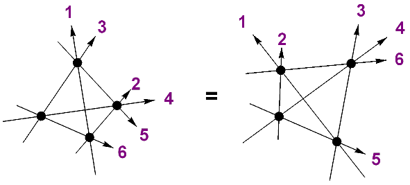
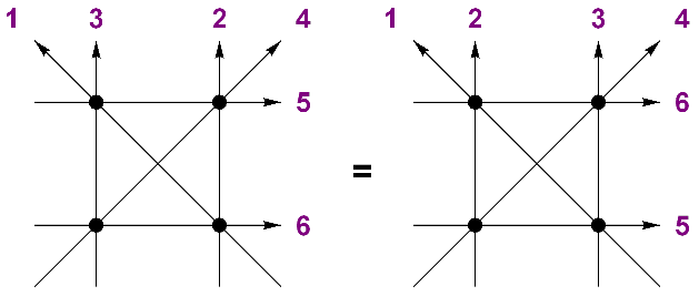
Figure 1. The diagram of the tetrahedron equation (2.5).

Figure 2. The projection of Figure 2 on planes.

The tetrahedron equation (2.5) is pictorially represented as Figure 2, where each straight line and vertex corresponds to $X$ and $\mathbf{R}$, respectively. Our tetrahedron equation (2.5) is motivated by the reduced expressions $\mathbf{i}=(1,3,2,1,3,2)$ and $(2,1,3,2,1,3)$ for the longest element of the Weyl group of $A_{3}$. See Remark 3.1. The correspondence between our tetrahedron equation (2.5) and the usual one $\mathbf{R}_{123}\mathbf{R}_{145}\mathbf{R}_{246}\mathbf{R}_{356}=\mathbf{R}_{356}\mathbf{R}_{246}\mathbf{R}_{145}\mathbf{R}_{123}$ will be presented in (2.6).

Examples of tetrahedron maps will be given in Section 3. In this paper, we mainly focus on tetrahedron maps defined on homogeneous spaces $X^{3}$ for simplicity, but Theorem 2.13 can be extended to inhomogeneous cases straightforwardly. We will deal with such a case in Section 3.3.

From now on, we mainly focus on involutive and symmetric tetrahedron maps defined as follows:

Definition 2.3.

We set a tetrahedron map by $\mathbf{R}:X^{3}\to X^{3}$. We call $\mathbf{R}$ involutive if it satisfies $\mathbf{R}^{2}=\mathrm{id}$, where $\mathrm{id}$ is the identity map.

Definition 2.4.

We set a tetrahedron map by $\mathbf{R}:X^{3}\to X^{3}$. We call $\mathbf{R}$ symmetric if it satisfies $\mathbf{R}_{123}=\mathbf{R}_{321}$.

These conditions are not strict. Actually, all examples of tetrahedron maps presented in Section 3 are involutive, and almost all of them are symmetric except $\mathcal{M}$ in Section 3.3.

Under these conditions, our tetrahedron equation (2.5) corresponds to the usual one as follows:

$$\begin{split}&\mathbf{R}_{245}\mathbf{R}_{135}\mathbf{R}_{126}\mathbf{R}_{346}=\mathbf{R}_{346}\mathbf{R}_{126}\mathbf{R}_{135}\mathbf{R}_{245},\\ \Longleftrightarrow{\ }&\mathbf{R}_{126}\mathbf{R}_{346}\mathbf{R}_{245}\mathbf{R}_{135}=\mathbf{R}_{135}\mathbf{R}_{245}\mathbf{R}_{346}\mathbf{R}_{126},\\ \Longleftrightarrow{\ }&\mathbf{R}_{621}\mathbf{R}_{643}\mathbf{R}_{245}\mathbf{R}_{135}=\mathbf{R}_{135}\mathbf{R}_{245}\mathbf{R}_{643}\mathbf{R}_{621},\end{split}$$ (2.6)

where we used the involutivity for the first line and the symmetry for the second line. Then, we obtain the usual tetrahedron equation by replacing indices as $1\to 3$, $3\to 5$, $5\to 6$ and $6\to 1$.

2.3. 3D reflection equation

In this paper, we only consider the 3D reflection equation[13] without spectral parameters. We define 3D reflection maps and their involutivity as with tetrahedron maps:

Definition 2.5.

Let $\mathbf{J}:X^{4}\to X^{4}$ denote a map. We set a tetrahedron map by $\mathbf{R}:X^{3}\to X^{3}$. We call $\mathbf{J}$ 3D reflection map if it satisfies the following 3D reflection equation on $X^{9}$:

$$\mathbf{R}_{489}\mathbf{J}_{3579}\mathbf{R}_{269}\mathbf{R}_{258}\mathbf{J}_{1678}\mathbf{J}_{1234}\mathbf{R}_{456}=\mathbf{R}_{456}\mathbf{J}_{1234}\mathbf{J}_{1678}\mathbf{R}_{258}\mathbf{R}_{269}\mathbf{J}_{3579}\mathbf{R}_{489},$$ (2.7)

where indices for $\mathbf{J}$ have the same meaning as ones given by Notation 2.1.

Definition 2.6.

We set a 3D reflection map by $\mathbf{J}:X^{4}\to X^{4}$. We call $\mathbf{J}$ involutive if it satisfies $\mathbf{J}^{2}=\mathrm{id}$.

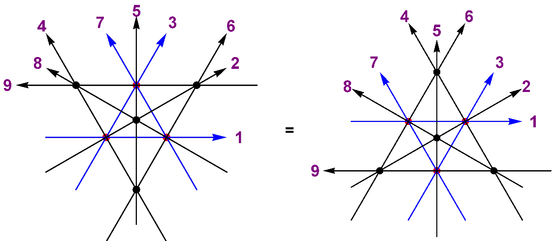
Figure 3. The diagram of the 3D reflection equation (2.7).

Figure 4. The projection of Figure 4 on the boundary plane.

The 3D reflection equation is pictorially represented as Figure 4, where each black and red vertex corresponds to $\mathbf{R}$ and $\mathbf{J}$, respectively. In the figure, each red vertex and blue line is on the light brown boundary plane, and each black line hits the plane and is reflected. It is notable that all lines in Figure 4 are straight. Such a figure is obtained by putting virtual half-opened book spines on blue lines and consider the intersections of the three books as $\mathbf{R}$, where such intersections are consequences from the elementary geometry. In Figure 4, such books are represented by translucent gray planes. See [20] for more detailed construction of Figure 4.

Examples of 3D reflection maps will be presented in Section 3 where all of them are involutive.

2.4. Condition and procedure for boundarization

We then proceed to the main part of this paper. We first introduce some definitions for the boundarization. For motivations for them, see Section 3.1.

Definition 2.7.

We set a tetrahedron map by $\mathbf{R}:X^{3}\to X^{3}$. We define a map $\mathbf{T}:X^{6}\to X^{6}$ by

$$\mathbf{T}=\mathbf{T}_{123456}=\mathbf{R}_{245}\mathbf{R}_{135}\mathbf{R}_{126}\mathbf{R}_{346}=\mathbf{R}_{346}\mathbf{R}_{126}\mathbf{R}_{135}\mathbf{R}_{245}.$$ (2.8)

We call $\mathbf{T}$ the tetrahedral composite of the tetrahedron map $\mathbf{R}$.

Definition 2.8.

We define a subset of $X^{6}$ by

$$Y=\{(x_{1},\cdots,x_{6})\mid x_{2}=x_{3},{\ }x_{5}=x_{6}\}.$$ (2.9)

We set $\phi:X^{4}\to Y$ and $\varphi:Y\to X^{4}$ by $\phi(x_{1},x_{2},x_{3},x_{4})=(x_{1},x_{2},x_{2},x_{3},x_{4},x_{4})$ and $\varphi(x_{1},x_{2},x_{2},x_{3},x_{4},x_{4})=(x_{1},x_{2},x_{3},x_{4})$, respectively. Apparently, they are bijections and satisfy $\phi^{-1}=\varphi$ and $\varphi^{-1}=\phi$.

Definition 2.9.

Let $\mathbf{R}:X^{3}\to X^{3}$ denote a tetrahedron map and $\mathbf{T}$ its tetrahedral composite. We call $\mathbf{R}$ boundarizable if the restriction of $\mathbf{T}$ to $Y$ gives a map on $Y$, that is, the following condition is satisfied:

$$\mathbf{x}\in Y{\ }\Longrightarrow{\ }\mathbf{T}(\mathbf{x})\in Y.$$ (2.10)

Definition 2.10.

Let $\mathbf{R}:X^{3}\to X^{3}$ denote a boundarizable tetrahedron map and $\mathbf{T}$ its tetrahedral composite. We define the boundarization $\mathbf{J}:X^{4}\to X^{4}$ of $\mathbf{R}$ by

$$\mathbf{J}(\mathbf{x})=\varphi(\mathbf{T}(\phi(\mathbf{x}))).$$ (2.11)

The boundarization given by (2.11) is pictorially represented as Figure 5, where each black and red vertex corresponds to $\mathbf{R}$ and $\mathbf{J}$, respectively.

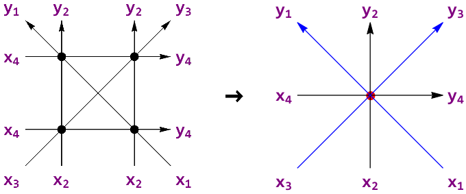
Figure 5. The diagram of boundarization given by (2.11) where we set $y_{i}=\varphi(\mathbf{T}(\phi(\mathbf{x})))_{i}$ and the $i$-th component of $\varphi(\mathbf{T}(\phi(\mathbf{x})))$ by $\varphi(\mathbf{T}(\phi(\mathbf{x})))_{i}$. See also Figure 2.

Proposition 2.11.

Let $\mathbf{R}:X^{3}\to X^{3}$ denote an involutive and boundarizable tetrahedron map and $\mathbf{J}$ its boundarization. Then, $\mathbf{J}$ is involutive.

Proof.

Let $\mathbf{T}$ denote the tetrahedral composite of $\mathbf{R}$. This is shown by the following direct calculation:

$$\mathbf{J}^{2}(\mathbf{x})=\varphi(\mathbf{T}(\phi(\varphi(\mathbf{T}(\phi(\mathbf{x}))))))=\varphi(\mathbf{T}(\mathbf{T}(\phi(\mathbf{x}))))=\varphi(\phi(\mathbf{x}))=\mathbf{x},$$ (2.12)

where we used $\phi^{-1}=\varphi$, $\varphi^{-1}=\phi$ and $\mathbf{T}^{2}=\mathbf{R}_{245}\mathbf{R}_{135}\mathbf{R}_{126}\mathbf{R}_{346}\mathbf{R}_{346}\mathbf{R}_{126}\mathbf{R}_{135}\mathbf{R}_{245}=\mathrm{id}$ by $\mathbf{R}^{2}=\mathrm{id}$. ∎

The following lemma is the heart of our construction, which is a three-dimensional analog of [8, (3.16)] and [21, (5)].

Lemma 2.12.

Let $\mathbf{R}$ denote an involutive and symmetric tetrahedron map. Then, we have the following identity on $X^{15}$:

$$\begin{split}&(\mathbf{R}_{489}\mathbf{R}_{\bar{4}\bar{8}\bar{9}})(\mathbf{R}_{579}\mathbf{R}_{3\bar{5}9}\mathbf{R}_{35\bar{9}}\mathbf{R}_{\bar{5}7\bar{9}})(\mathbf{R}_{26\bar{9}}\mathbf{R}_{\bar{2}\bar{6}9})(\mathbf{R}_{2\bar{5}8}\mathbf{R}_{\bar{2}5\bar{8}})\\ &\hskip 30.00005pt\times(\mathbf{R}_{\bar{6}7\bar{8}}\mathbf{R}_{16\bar{8}}\mathbf{R}_{1\bar{6}8}\mathbf{R}_{678})(\mathbf{R}_{234}\mathbf{R}_{1\bar{2}4}\mathbf{R}_{12\bar{4}}\mathbf{R}_{\bar{2}3\bar{4}})(\mathbf{R}_{\bar{4}\bar{5}\bar{6}}\mathbf{R}_{456})\\ &=(\mathbf{R}_{456}\mathbf{R}_{\bar{4}\bar{5}\bar{6}})(\mathbf{R}_{234}\mathbf{R}_{1\bar{2}4}\mathbf{R}_{12\bar{4}}\mathbf{R}_{\bar{2}3\bar{4}})(\mathbf{R}_{\bar{6}7\bar{8}}\mathbf{R}_{16\bar{8}}\mathbf{R}_{1\bar{6}8}\mathbf{R}_{678})\\ &\hskip 30.00005pt\times(\mathbf{R}_{\bar{2}5\bar{8}}\mathbf{R}_{2\bar{5}8})(\mathbf{R}_{\bar{2}\bar{6}9}\mathbf{R}_{26\bar{9}})(\mathbf{R}_{579}\mathbf{R}_{3\bar{5}9}\mathbf{R}_{35\bar{9}}\mathbf{R}_{\bar{5}7\bar{9}})(\mathbf{R}_{\bar{4}\bar{8}\bar{9}}\mathbf{R}_{489}).\end{split}$$ (2.13)

Proof.

The proof is done by simply repeated uses of the tetrahedron equation with the involutivity and symmetry for $\mathbf{R}$. The detail of the calculation is available in Appendix A, where we put the underlines to the parts to be got together or deformed. ∎

For inhomogeneous cases, not all tetrahedron maps in (2.13) need to be symmetric. See Lemma 3.7 for an example.

The identity (2.13) is pictorially represented as Figure 7, where each vertex corresponds to $\mathbf{R}$. In the figure, black and red vertices are above the translucent light brown plane, and brown and orange ones are below the plane. As with Figure 4, it is notable that all lines in Figure 7 are straight, which is also a consequence from the elementary geometry but we omit it because it is beyond the scope of this paper.

In Figure 7, brown vertices are interpreted as the mirrored image of black ones, and red and orange vertices will be boundarized to $\mathbf{J}$. This interpretation is theorized as follows, which is the main result of this paper.

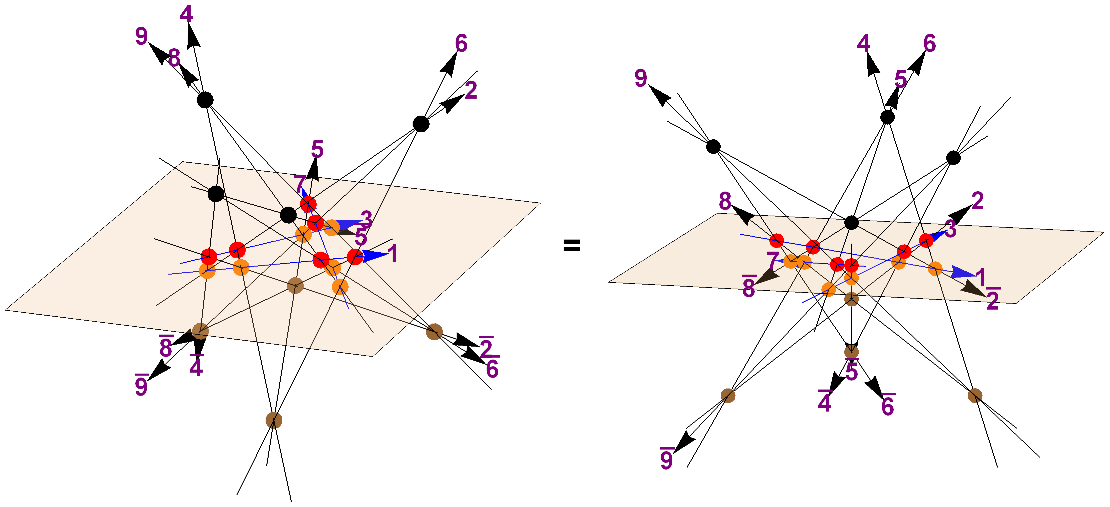
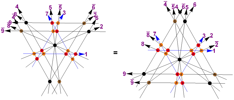
Figure 6. The diagram of the identity (2.13).

Figure 7. The projection of Figure 7 on the boundary plane.

Theorem 2.13.

Let $\mathbf{R}:X^{3}\to X^{3}$ denote an involutive, symmetric and boundarizable tetrahedron map and $\mathbf{J}:X^{4}\to X^{4}$ its boundarization. Then, they satisfy the 3D reflection equation (2.7).

Proof.

Let $\mathbf{T}$ denote the tetrahedral composite of $\mathbf{R}$. By using $\mathbf{T}$, (2.13) is written as follows:

$$\begin{split}&(\mathbf{R}_{489}\mathbf{R}_{\bar{4}\bar{8}\bar{9}})\mathbf{T}_{35\bar{5}79\bar{9}}(\mathbf{R}_{26\bar{9}}\mathbf{R}_{\bar{2}\bar{6}9})(\mathbf{R}_{2\bar{5}8}\mathbf{R}_{\bar{2}5\bar{8}})\mathbf{T}_{16\bar{6}78\bar{8}}\mathbf{T}_{12\bar{2}34\bar{4}}(\mathbf{R}_{\bar{4}\bar{5}\bar{6}}\mathbf{R}_{456})\\ &=(\mathbf{R}_{456}\mathbf{R}_{\bar{4}\bar{5}\bar{6}})\mathbf{T}_{12\bar{2}34\bar{4}}\mathbf{T}_{16\bar{6}78\bar{8}}(\mathbf{R}_{\bar{2}5\bar{8}}\mathbf{R}_{2\bar{5}8})(\mathbf{R}_{\bar{2}\bar{6}9}\mathbf{R}_{26\bar{9}})\mathbf{T}_{35\bar{5}79\bar{9}}(\mathbf{R}_{\bar{4}\bar{8}\bar{9}}\mathbf{R}_{489}),\end{split}$$ (2.14)

where we assume that spaces are ordered as

$$1\times 2\times\bar{2}\times 3\times 4\times\bar{4}\times 5\times\bar{5}\times 6\times\bar{6}\times 7\times 8\times\bar{8}\times 9\times\bar{9}.$$ (2.15)

Let us act both sides of (2.14) on

$$(x_{1},x_{2},x_{2},x_{3},x_{4},x_{4},x_{5},x_{5},x_{6},x_{6},x_{7},x_{8},x_{8},x_{9},x_{9}).$$ (2.16)

In that case, by using (2.10), it is easy to see that all $\mathbf{T}$ in (2.14) receive elements of $Y$ as inputs. By considering (2.11), we then obtain the desired 3D reflection equation just viewing the upper side of the plane of Figure 7. This is in the same way as the proof of [21, Theorem 7].

More formally, this can be shown by applying cutting and reconnection procedure to (2.14) given by

$$\mathbf{T}_{ij\bar{j}kl\bar{l}}\mapsto P_{j\bar{j}}P_{l\bar{l}}\mathbf{J}_{ijkl}\mathbf{J}_{\bar{i}\bar{j}\bar{k}\bar{l}},$$ (2.17)

where we introduce new spaces $\bar{i}$ and $\bar{k}$ which are copies of the first and third spaces, respectively. We assume that they receive the same inputs to $i$ and $k$, respectively, and the connectivity for $\bar{i}$ and $\bar{k}$ will be given as (2.18). The part $P_{j\bar{j}}P_{l\bar{l}}$ gives “reconnection”, which does not change the outputs of (2.14) because all $\mathbf{T}$ in (2.14) output elements of $Y$ by (2.10). The procedure (2.17) is pictorially represented as Figure 8.

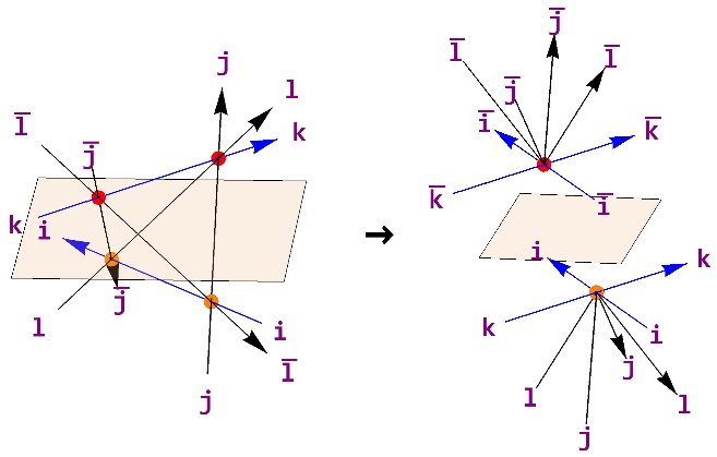
Figure 8. The diagram of cutting and reconnection procedure given in the proof of Theorem 2.13.

By applying (2.17) to both sides of (2.14), we obtain

$$\begin{split}&(\mathbf{R}_{489}\mathbf{R}_{\bar{4}\bar{8}\bar{9}})(P_{5\bar{5}}P_{9\bar{9}}\mathbf{J}_{3579}\mathbf{J}_{\bar{3}\bar{5}\bar{7}\bar{9}})(\mathbf{R}_{26\bar{9}}\mathbf{R}_{\bar{2}\bar{6}9})(\mathbf{R}_{2\bar{5}8}\mathbf{R}_{\bar{2}5\bar{8}})\\ &\hskip 30.00005pt\times(P_{6\bar{6}}P_{8\bar{8}}\mathbf{J}_{1678}\mathbf{J}_{\bar{1}\bar{6}\bar{7}\bar{8}})(P_{2\bar{2}}P_{4\bar{4}}\mathbf{J}_{1234}\mathbf{J}_{\bar{1}\bar{2}\bar{3}\bar{4}})(\mathbf{R}_{\bar{4}\bar{5}\bar{6}}\mathbf{R}_{456})\\ &=(\mathbf{R}_{456}\mathbf{R}_{\bar{4}\bar{5}\bar{6}})(P_{2\bar{2}}P_{4\bar{4}}\mathbf{J}_{1234}\mathbf{J}_{\bar{1}\bar{2}\bar{3}\bar{4}})(P_{6\bar{6}}P_{8\bar{8}}\mathbf{J}_{1678}\mathbf{J}_{\bar{1}\bar{6}\bar{7}\bar{8}})\\ &\hskip 30.00005pt\times(\mathbf{R}_{\bar{2}5\bar{8}}\mathbf{R}_{2\bar{5}8})(\mathbf{R}_{\bar{2}\bar{6}9}\mathbf{R}_{26\bar{9}})(P_{5\bar{5}}P_{9\bar{9}}\mathbf{J}_{3579}\mathbf{J}_{\bar{3}\bar{5}\bar{7}\bar{9}})(\mathbf{R}_{\bar{4}\bar{8}\bar{9}}\mathbf{R}_{489}).\end{split}$$ (2.18)

By eliminating $P_{i\bar{i}}$, this is rewritten as follows:

$$\begin{split}&(\mathbf{R}_{489}\mathbf{R}_{\bar{4}\bar{8}\bar{9}})(\mathbf{J}_{3579}\mathbf{J}_{\bar{3}\bar{5}\bar{7}\bar{9}})(\mathbf{R}_{269}\mathbf{R}_{\bar{2}\bar{6}\bar{9}})(\mathbf{R}_{258}\mathbf{R}_{\bar{2}\bar{5}\bar{8}})(\mathbf{J}_{1678}\mathbf{J}_{\bar{1}\bar{6}\bar{7}\bar{8}})(\mathbf{J}_{1234}\mathbf{J}_{\bar{1}\bar{2}\bar{3}\bar{4}})(\mathbf{R}_{\bar{4}\bar{5}\bar{6}}\mathbf{R}_{456})\\ &=(\mathbf{R}_{456}\mathbf{R}_{\bar{4}\bar{5}\bar{6}})(\mathbf{J}_{1234}\mathbf{J}_{\bar{1}\bar{2}\bar{3}\bar{4}})(\mathbf{J}_{1678}\mathbf{J}_{\bar{1}\bar{6}\bar{7}\bar{8}})(\mathbf{R}_{258}\mathbf{R}_{\bar{2}\bar{5}\bar{8}})(\mathbf{R}_{269}\mathbf{R}_{\bar{2}\bar{6}\bar{9}})(\mathbf{J}_{3579}\mathbf{J}_{\bar{3}\bar{5}\bar{7}\bar{9}})(\mathbf{R}_{\bar{4}\bar{8}\bar{9}}\mathbf{R}_{489}).\end{split}$$ (2.19)

This is exactly the direct product of the 3D reflection equation. We then obtain the desired result. ∎

3. Examples

3.1. Birational and combinatorial transition map

Let $\mathbb{R}_{>0}$ denote the set of positive real numbers. We set $\mathbf{R}:\mathbb{R}_{>0}^{3}\to\mathbb{R}_{>0}^{3}$ by

$$\mathbf{R}:(x_{1},x_{2},x_{3})\mapsto\left(\frac{x_{1}x_{2}}{x_{1}+x_{3}},x_{1}+x_{3},\frac{x_{2}x_{3}}{x_{1}+x_{3}}\right).$$ (3.1)

Then, the map (3.1) is the involutive and symmetric tetrahedron map. This solution was obtained by [30, (36)]. Recently, this was also derived[17, (41)] by considering semi-invariants for discrete AKP equation, which appears in ABS classification as $\chi_{1}$[1].

We can verify $\mathbf{R}$ satisfies (2.10) by direct calculations, so it is boundarizable. The associated boundarization $\mathbf{J}:\mathbb{R}_{>0}^{4}\to\mathbb{R}_{>0}^{4}$ is explicitly obtained as follows:

$$\begin{split}&\mathbf{J}:(x_{1},x_{2},x_{3},x_{4})\mapsto\left(\frac{x_{1}x_{2}^{2}x_{3}}{y_{1}},\frac{y_{1}}{y_{2}},\frac{y_{2}^{2}}{y_{1}},\frac{x_{2}x_{3}x_{4}}{y_{2}}\right),\\ &y_{1}=x_{1}(x_{2}+x_{4})^{2}+x_{3}x_{4}^{2},\quad y_{2}=x_{1}(x_{2}+x_{4})+x_{3}x_{4}.\end{split}$$ (3.2)

Then, $(\mathbf{R},\mathbf{J})$ satisfies the 3D reflection equation (2.7) by Theorem 2.13. This is actually the known solution[19, 20]. See Remark 3.1 and 3.2.

Algebraic aspects for the solution (3.1) are deeply understood for now. The formula (3.1) has also appeared in [27, Proposition 2.5] independently, where it was characterized as the transition map of parametrizations of the totally positive part of the special linear group $SL_{3}$. Explicit formulae for such transition maps were also obtained for any semisimple Lie groups, and they all have the combinatorial counterpart via the tropical limit[5]. For example, the map (3.1) with $ab\to a+b$ and $a+b\to\min(a,b)$ gives the following map on $\mathbb{Z}_{\geq 0}^{3}$[25, 2.1]:

$$\mathcal{R}:(x_{1},x_{2},x_{3})\mapsto\left(x_{1}+x_{2}-\min(x_{1},x_{3}),\min(x_{1},x_{3}),x_{2}+x_{3}-\min(x_{1},x_{3})\right).$$ (3.3)

This also gives the involutive and symmetric tetrahedron map. Generally, it is known that the tropical limit of such transition maps gives the transition map of Lusztig’s parametrizations of the canonical basis of the Drinfeld-Jimbo quantum algebra $U_{q}(\mathfrak{g})$. The map (3.3) is the example for the case $\mathfrak{g}=sl_{3}$.

Note that the 3D reflection map (3.2) also admits the tropical limit, which is given by the following map on $\mathbb{Z}_{\geq 0}^{4}$:

$$\begin{split}&\mathcal{J}:(x_{1},x_{2},x_{3},x_{4})\mapsto\left(x_{1}+2x_{2}+x_{3}-y_{1},y_{1}-y_{2},2y_{2}-y_{1},x_{2}+x_{3}+x_{4}-y_{2}\right),\\ &y_{1}=\min(x_{1}+2\min(x_{2},x_{4}),x_{3}+2x_{4}),\\ &y_{2}=\min(x_{1}+\min(x_{2},x_{4}),x_{3}+x_{4}).\end{split}$$ (3.4)

This is also the involutive 3D reflection map, that is, $(\mathcal{R},\mathcal{J})$ satisfies the following 3D reflection equation:

$$\mathcal{R}_{489}\mathcal{J}_{3579}\mathcal{R}_{269}\mathcal{R}_{258}\mathcal{J}_{1678}\mathcal{J}_{1234}\mathcal{R}_{456}=\mathcal{R}_{456}\mathcal{J}_{1234}\mathcal{J}_{1678}\mathcal{R}_{258}\mathcal{R}_{269}\mathcal{J}_{3579}\mathcal{R}_{489}.$$ (3.5)

This is due to the fact that the 3D reflection map (3.2) has a similar algebraic origin to the tetrahedron map (3.1). Actually, these maps (3.1) and (3.2) are 3DR and 3DJ referered in Section 1, respevtively. See Remark 3.1.

Remark 3.1.

The 3D reflection map (3.2) is exactly the transition map of parametrizations of the totally positive part of the special orthogonal group $SO_{5}$ just as the tetrahedron map (3.1) is one of $SL_{3}$. This is due to the fact[5, 26] that the boundarization relation (2.11) for these maps is exactly the relation obtained via folding the Dynkin diagram of $A_{3}$ into one of $B_{2}$. Here, it is crucial that the transition map for $SL_{4}$ is given by the tetrahedral composite of $\mathbf{R}$ like [19, (2.44),(2.45)], which is associated with the reduced expressions $\mathbf{i}=(1,3,2,1,3,2)$ and $(2,1,3,2,1,3)$ for the longest element of the Weyl group of $A_{3}$. This result is one of the main motivations for this study as explained in Section 1.

The relation between $\mathbf{R}$ and $\mathbf{J}$ was first observed by Lusztig[26, 12.5] and formally mentioned by [5, Proof of Theorem 5.2]. Later, Lusztig gave the detailed derivation of the above proposition in terms of Dynkin diagram automorphisms[28, 1.9], and further developments are recently given by [34].

Remark 3.2.

The quantum counterparts for the maps (3.3) and (3.4) are also known[15, 20], which are the solutions to the tetrahedron and 3D reflection equation for matrices. They are obtained as the intertwiners of irreducible representations of the quantum coodinate rings $A_{q}(SL_{3})$[15, 1.12(c)] and $A_{q}(SO_{5})$[20, Theorem 4.2], respectively. It is remarkable that they are also characterized as the transition matrices of PBW bases of the nilpotent subalgebra of the quantum alegbras $U_{q}(sl_{3})$ and $U_{q}(so_{5})$, respectively[23].

The fact that the maps (3.1) and (3.2) satisfy the 3D reflection equation (2.7) was found as a by-product in the process of seeking for a geometric counterpart of such intertwiners[19], although the maps (3.1) and (3.2) themselves are known long before these developments.

3.2. Sergeev’s electrical solution

Here, we assume all variables are generic. For $\lambda\in\mathbb{C}$, we set $\mathbf{R}(\lambda):\mathbb{C}^{3}\to\mathbb{C}^{3}$ by

$$\mathbf{R}(\lambda):(x_{1},x_{2},x_{3})\mapsto\left(\frac{x_{1}x_{2}}{x_{1}+x_{3}+\lambda x_{1}x_{2}x_{3}},x_{1}+x_{3}+\lambda x_{1}x_{2}x_{3},\frac{x_{2}x_{3}}{x_{1}+x_{3}+\lambda x_{1}x_{2}x_{3}}\right).$$ (3.6)

Then, the map (3.6) is involutive and symmetric, and satisfies the following tetrahedron equation:

$$\mathbf{R}(\lambda)_{245}\mathbf{R}(\lambda)_{135}\mathbf{R}(\lambda)_{126}\mathbf{R}(\lambda)_{346}=\mathbf{R}(\lambda)_{346}\mathbf{R}(\lambda)_{126}\mathbf{R}(\lambda)_{135}\mathbf{R}(\lambda)_{245}.$$ (3.7)

Apparently, this solution is a one-parametric generalization of (3.1). Note that we can obtain (3.6) from the case $\lambda=1$ by using simple component-wise similarity transformations, so the scale of $\lambda$ does not matter. The case for $\lambda=1$ was first obtained by [30, (28)] (see also [16]) and later the parametric representation (3.6) was introduced by [24, Section 4, Remark] from an algebraic point of view. As mentioned by [30], it is associated with the electric network transformation, so often called the electrical solution, and so on. Interestingly, this solution was also derived[17, (43)] associated with discrete BKP equation just as (3.1) is associated with discrete AKP equation.

We can verify $\mathbf{R}(\lambda)$ satisfies (2.10) by dicrect calculations, so it is boundarizable. The associated boundarization $\mathbf{J}(\lambda):\mathbb{C}^{4}\to\mathbb{C}^{4}$ is explicitly obtained as follows:

$$\begin{split}&\mathbf{J}(\lambda):(x_{1},x_{2},x_{3},x_{4})\mapsto\left(\frac{x_{1}x_{2}^{2}x_{3}}{y_{1}},\frac{y_{1}}{y_{2}},\frac{y_{2}^{2}}{y_{1}},\frac{x_{2}x_{3}x_{4}}{y_{2}}\right),\\ &y_{1}=x_{1}(x_{2}+x_{4})(x_{2}+x_{4}+2\lambda x_{2}x_{3}x_{4})+x_{3}x_{4}^{2},\\ &y_{2}=x_{1}(x_{2}+x_{4}+2\lambda x_{2}x_{3}x_{4})+x_{3}x_{4}.\end{split}$$ (3.8)

Similarly to (3.6), this gives (3.2) when we set $\lambda=0$. We note that the formula (3.8) appears in [24, Section 5, Remark] without any derivations. We hope that our result gives a new insight into the topic about electrical Lie groups. By Theorem 2.13, $(\mathbf{R}(\lambda),\mathbf{J}(\lambda))$ gives a new solution to the 3D reflection equation, which is a one-parametric generalization of one of Section 3.1:

Proposition 3.3.

$$\begin{split}&\mathbf{R}(\lambda)_{489}\mathbf{J}(\lambda)_{3579}\mathbf{R}(\lambda)_{269}\mathbf{R}(\lambda)_{258}\mathbf{J}(\lambda)_{1678}\mathbf{J}(\lambda)_{1234}\mathbf{R}(\lambda)_{456}\\ &=\mathbf{R}(\lambda)_{456}\mathbf{J}(\lambda)_{1234}\mathbf{J}(\lambda)_{1678}\mathbf{R}(\lambda)_{258}\mathbf{R}(\lambda)_{269}\mathbf{J}(\lambda)_{3579}\mathbf{R}(\lambda)_{489}.\end{split}$$ (3.9)

3.3. Super analog of combinatorial transition map

In this section, we present an inhomogeneous extension of Theorem 2.13. We set $\mathcal{M}:\mathbb{Z}_{\geq 0}\times\{0,1\}\times\{0,1\}\to\mathbb{Z}_{\geq 0}\times\{0,1\}\times\{0,1\}$ and $\mathcal{N}:\{0,1\}\times\mathbb{Z}_{\geq 0}\times\{0,1\}\to\{0,1\}\times\mathbb{Z}_{\geq 0}\times\{0,1\}$ by

$$\mathcal{M}:(x_{1},x_{2},x_{3})\mapsto\left(x_{1}+x_{2}-v,v,x_{2}+x_{3}-v\right),$$ (3.10)

$$\mathcal{N}:(x_{1},x_{2},x_{3})\mapsto\left(x_{1}+w,x_{2}-w,x_{3}+w\right),$$ (3.11)

where we set $v=\min(x_{1}+x_{2},x_{3})$ and $w=\min(x_{2},1-x_{1}-x_{3})$. Then, both of them are involutive and the map (3.11) is also symmetric. They satisfy the following tetrahedron equations on $\mathbb{Z}_{\geq 0}\times\{0,1\}^{2}\times\mathbb{Z}_{\geq 0}\times\{0,1\}^{2}$ and $\mathbb{Z}_{\geq 0}^{3}\times\{0,1\}^{3}$, respectively:

Lemma 3.4.

$$\mathcal{N}_{245}\mathcal{M}_{135}\mathcal{M}_{126}\mathcal{N}_{346} =\mathcal{N}_{346}\mathcal{M}_{126}\mathcal{M}_{135}\mathcal{N}_{245},$$ (3.12)

$$\mathcal{R}_{123}\mathcal{M}_{145}\mathcal{M}_{246}\mathcal{M}_{356} =\mathcal{M}_{356}\mathcal{M}_{246}\mathcal{M}_{145}\mathcal{R}_{123},$$ (3.13)

where $\mathcal{R}$ is given by (3.3).

Proof.

The second equation (3.13) is exactly [36, Corollary 6.6]. The first equation (3.12) can be proved by exhaustion on values of the subspace $\{0,1\}^{4}$. For example, if we apply the both sides of (3.12) to $(x_{1},0,0,x_{4},0,0){\ }(x_{1},x_{4}\in\mathbb{Z}_{\geq 0})$, they are calculated as follows:

1. The case $x_{1},x_{4}\geq 1$.

   $$\begin{split}(x_{1},0,0,x_{4},0,0)&\overset{\mathcal{N}_{346}}{\mapsto}(x_{1},0,1,x_{4}-1,0,1)\overset{\mathcal{M}_{126}}{\mapsto}(x_{1}-1,1,1,x_{4}-1,0,0)\\ &\overset{\mathcal{M}_{135}}{\mapsto}(x_{1},1,0,x_{4}-1,1,0)\overset{\mathcal{N}_{245}}{\mapsto}(x_{1},0,0,x_{4},0,0),\end{split}$$ (3.14)

   $$\begin{split}(x_{1},0,0,x_{4},0,0)&\overset{\mathcal{N}_{245}}{\mapsto}(x_{1},1,0,x_{4}-1,1,0)\overset{\mathcal{M}_{135}}{\mapsto}(x_{1}-1,1,1,x_{4}-1,0,0)\\ &\overset{\mathcal{M}_{126}}{\mapsto}(x_{1},0,1,x_{4}-1,0,1)\overset{\mathcal{N}_{346}}{\mapsto}(x_{1},0,0,x_{4},0,0).\end{split}$$ (3.15)

2. The case $x_{1}=0$ and $x_{4}\geq 1$.

   $$\begin{split}(0,0,0,x_{4},0,0)&\overset{\mathcal{N}_{346}}{\mapsto}(0,0,1,x_{4}-1,0,1)\overset{\mathcal{M}_{126}}{\mapsto}(0,0,1,x_{4}-1,0,1)\\ &\overset{\mathcal{M}_{135}}{\mapsto}(1,0,0,x_{4}-1,1,1)\overset{\mathcal{N}_{245}}{\mapsto}(1,0,0,x_{4}-1,1,1),\end{split}$$ (3.16)

   $$\begin{split}(0,0,0,x_{4},0,0)&\overset{\mathcal{N}_{245}}{\mapsto}(0,1,0,x_{4}-1,1,0)\overset{\mathcal{M}_{135}}{\mapsto}(0,1,0,x_{4}-1,1,0)\\ &\overset{\mathcal{M}_{126}}{\mapsto}(1,0,0,x_{4}-1,1,1)\overset{\mathcal{N}_{346}}{\mapsto}(1,0,0,x_{4}-1,1,1).\end{split}$$ (3.17)

3. The case $x_{1}\geq 0$ and $x_{4}=0$.

   $$\begin{split}(x_{1},0,0,0,0,0)&\overset{\mathcal{N}_{346}}{\mapsto}(x_{1},0,0,0,0,0)\overset{\mathcal{M}_{126}}{\mapsto}(x_{1},0,0,0,0,0)\\ &\overset{\mathcal{M}_{135}}{\mapsto}(x_{1},0,0,0,0,0)\overset{\mathcal{N}_{245}}{\mapsto}(x_{1},0,0,0,0,0),\end{split}$$ (3.18)

   $$\begin{split}(x_{1},0,0,0,0,0)&\overset{\mathcal{N}_{245}}{\mapsto}(x_{1},0,0,0,0,0)\overset{\mathcal{M}_{135}}{\mapsto}(x_{1},0,0,0,0,0)\\ &\overset{\mathcal{M}_{126}}{\mapsto}(x_{1},0,0,0,0,0)\overset{\mathcal{N}_{346}}{\mapsto}(x_{1},0,0,0,0,0).\end{split}$$ (3.19)

They give (3.12) for the case $(0,0,0,0)\in\{0,1\}^{4}$. ∎

The maps (3.10) and (3.11) were obtained by considering the crystal limit of the transition matrices of PBW bases of the nilpotent subalgebra of the quantum superalgebras of type A[36, Sec 6.1], so they are natural analogs of the tetrahedron map (3.3).

Lemma 3.5.

The tetrahedral composite $\mathcal{T}=\mathcal{N}_{245}\mathcal{M}_{135}\mathcal{M}_{126}\mathcal{N}_{346}$ on $\mathbb{Z}_{\geq 0}\times\{0,1\}^{2}\times\mathbb{Z}_{\geq 0}\times\{0,1\}^{2}$ satisfies the boundarization condition (2.10).

Proof.

This can be proved by exhaustion. For example, (3.14), (3.16) and (3.18) verify the case $x_{2}=x_{3}=x_{5}=x_{6}=0$. ∎

Let $\mathcal{X}$ denote a map on $\mathbb{Z}_{\geq 0}\times\{0,1\}\times\mathbb{Z}_{\geq 0}\times\{0,1\}$ given by

$$\begin{split}&\mathcal{X}:(x_{1},x_{2},x_{3},x_{4})\mapsto\left(x_{1}+2x_{2}+x_{3}-y_{1},y_{1}-y_{2},2y_{2}-y_{1},x_{2}+x_{3}+x_{4}-y_{2}\right),\\ &y_{1}=\max(x_{3}+\min(x_{1}+2x_{2}+x_{4}-1,2x_{4}),0),\\ &y_{2}=\max(x_{3}+\min(x_{1}+x_{2}+x_{4}-1,x_{4}),0).\end{split}$$ (3.20)

The map (3.20) was obtained by [36, Sec 6.1]. The origin of it is similar to the maps (3.10) and (3.11): it is obtained by considering the crystal limit of the transition matrix for the quantum superalgebras of type B, so a natural analog of the 3D reflection map (3.4). As shown in [36], the map (3.20) is involutive.

We have a super analog of the relation which mentioned in Remark 3.1 by exhaustion:

Proposition 3.6.

The boundarization associated with the tetrahedral composite $\mathcal{T}=\mathcal{N}_{245}\mathcal{M}_{135}\mathcal{M}_{126}\mathcal{N}_{346}$ is given by $\mathcal{X}$.

Then, we present an inhomogeneous extension of Lemma 2.12.

Lemma 3.7.

$$\begin{split}&(\mathcal{M}_{489}\mathcal{M}_{\bar{4}\bar{8}\bar{9}})(\mathcal{N}_{579}\mathcal{M}_{3\bar{5}9}\mathcal{M}_{35\bar{9}}\mathcal{N}_{\bar{5}7\bar{9}})(\mathcal{M}_{26\bar{9}}\mathcal{M}_{\bar{2}\bar{6}9})(\mathcal{M}_{2\bar{5}8}\mathcal{M}_{\bar{2}5\bar{8}})\\ &\hskip 30.00005pt\times(\mathcal{N}_{\bar{6}7\bar{8}}\mathcal{M}_{16\bar{8}}\mathcal{M}_{1\bar{6}8}\mathcal{N}_{678})(\mathcal{R}_{234}\mathcal{R}_{1\bar{2}4}\mathcal{R}_{12\bar{4}}\mathcal{R}_{\bar{2}3\bar{4}})(\mathcal{M}_{\bar{4}\bar{5}\bar{6}}\mathcal{M}_{456})\\ &=(\mathcal{M}_{456}\mathcal{M}_{\bar{4}\bar{5}\bar{6}})(\mathcal{R}_{234}\mathcal{R}_{1\bar{2}4}\mathcal{R}_{12\bar{4}}\mathcal{R}_{\bar{2}3\bar{4}})(\mathcal{N}_{\bar{6}7\bar{8}}\mathcal{M}_{16\bar{8}}\mathcal{M}_{1\bar{6}8}\mathcal{N}_{678})\\ &\hskip 30.00005pt\times(\mathcal{M}_{\bar{2}5\bar{8}}\mathcal{M}_{2\bar{5}8})(\mathcal{M}_{\bar{2}\bar{6}9}\mathcal{M}_{26\bar{9}})(\mathcal{N}_{579}\mathcal{M}_{3\bar{5}9}\mathcal{M}_{35\bar{9}}\mathcal{N}_{\bar{5}7\bar{9}})(\mathcal{M}_{\bar{4}\bar{8}\bar{9}}\mathcal{M}_{489}),\end{split}$$ (3.21)

where $\mathcal{R}$ is given by (3.3).

Proof.

This is shown in the same way as Lemma 2.12. The detail of the calculation is available in Appendix B, where we put the underlines to the parts to be got together or deformed. As we can see by Appendix B, we do not need the symmetry for $\mathcal{M}$. ∎

By using the above lemmas, proposition and the properties for $(\mathcal{R},\mathcal{J})$, we obtain the following solution to the 3D reflection equation:

Theorem 3.8.

$$\mathcal{M}_{489}\mathcal{X}_{3579}\mathcal{M}_{269}\mathcal{M}_{258}\mathcal{X}_{1678}\mathcal{J}_{1234}\mathcal{M}_{456}=\mathcal{M}_{456}\mathcal{J}_{1234}\mathcal{X}_{1678}\mathcal{M}_{258}\mathcal{M}_{269}\mathcal{X}_{3579}\mathcal{M}_{489}.$$ (3.22)

Proof.

This is shown in the same way as Theorem 2.13. ∎

Note that the solution (3.22) has already obtained[36, (6.33)], but our construction gives an alternative derivation for this solution.

3.4. Two-component solution associated with soliton equation

Here, we assume all variables are generic. We set $\mathbf{R}:(\mathbb{C}^{2})^{3}\to(\mathbb{C}^{2})^{3}$ by

$$\mathbf{R}:\left(\begin{pmatrix}x_{1}\\ y_{1}\end{pmatrix},\begin{pmatrix}x_{2}\\ y_{2}\end{pmatrix},\begin{pmatrix}x_{3}\\ y_{3}\end{pmatrix}\right)\mapsto\left(\begin{pmatrix}\displaystyle\frac{x_{1}x_{2}}{x_{1}+x_{3}}\\ \\ \displaystyle\frac{(x_{1}+x_{3})y_{1}y_{2}}{x_{1}y_{1}+x_{3}y_{3}}\end{pmatrix},\begin{pmatrix}\displaystyle x_{1}+x_{3}\\ \\ \displaystyle\frac{x_{1}y_{1}+x_{3}y_{3}}{x_{1}+x_{3}}\end{pmatrix},\begin{pmatrix}\displaystyle\frac{x_{2}x_{3}}{x_{1}+x_{3}}\\ \\ \displaystyle\frac{(x_{1}+x_{3})y_{2}y_{3}}{x_{1}y_{1}+x_{3}y_{3}}\end{pmatrix}\right).$$ (3.23)

Then, the map (3.23) is the involutive and symmetric tetrahedron map. This solution was obtained[17, (93)] associated with discrete modified KP equation, which appears in ABS classification as $\chi_{4}$[1]. This solution is a two-component generalization of (3.1) because this gives (3.1) when we set $y_{i}=1{\ }(i=1,2,3)$.

We can verify $\mathbf{R}$ satisfies (2.10) by direct calculations, so it is boundarizable. The associated boundarization $\mathbf{J}:(\mathbb{C}^{2})^{4}\to(\mathbb{C}^{2})^{4}$ is explicitly obtained as follows:

$$\begin{split}&\mathbf{J}:\left(\begin{pmatrix}x_{1}\\ y_{1}\end{pmatrix},\begin{pmatrix}x_{2}\\ y_{2}\end{pmatrix},\begin{pmatrix}x_{3}\\ y_{3}\end{pmatrix},\begin{pmatrix}x_{4}\\ y_{4}\end{pmatrix}\right)\mapsto\left(\begin{pmatrix}\displaystyle\frac{x_{1}x_{2}^{2}x_{3}}{z_{1}}\\ \\ \displaystyle\frac{y_{1}y_{2}^{2}y_{3}z_{1}}{w_{1}}\end{pmatrix},\begin{pmatrix}\displaystyle\frac{z_{1}}{z_{2}}\\ \\ \displaystyle\frac{z_{2}w_{1}}{z_{1}w_{2}}\end{pmatrix},\begin{pmatrix}\displaystyle\frac{z_{2}^{2}}{z_{1}}\\ \\ \displaystyle\frac{z_{1}w_{2}^{2}}{z_{2}^{2}w_{1}}\end{pmatrix},\begin{pmatrix}\displaystyle\frac{x_{2}x_{3}x_{4}}{z_{2}}\\ \\ \displaystyle\frac{y_{2}y_{3}y_{4}z_{2}}{w_{2}}\end{pmatrix}\right),\\ &z_{1}=x_{1}(x_{2}+x_{4})^{2}+x_{3}x_{4}^{2},\quad z_{2}=x_{1}(x_{2}+x_{4})+x_{3}x_{4},\\ &w_{1}=x_{1}y_{1}(x_{2}y_{2}+x_{4}y_{4})^{2}+x_{3}x_{4}^{2}y_{3}y_{4}^{2},\quad w_{2}=x_{1}y_{1}(x_{2}y_{2}+x_{4}y_{4})+x_{3}x_{4}y_{3}y_{4}.\end{split}$$ (3.24)

Similarly to (3.23), this gives (3.2) when we set $y_{i}=1{\ }(i=1,2,3,4)$. By Theorem 2.13, $(\mathbf{R},\mathbf{J})$ gives a new solution to the 3D reflection equation, which is a two-component generalization of one of Section 3.1:

Proposition 3.9.

$(\mathbf{R},\mathbf{J})$ given by (3.23) and (3.24) satisfies the 3D reflection equation (2.7).

Appendix A Proof of Lemma 2.12

$$\mathbf{R}_{489}\mathbf{R}_{\bar{4}\bar{8}\bar{9}}\underline{\mathbf{R}_{579}\mathbf{R}_{3\bar{5}9}\mathbf{R}_{35\bar{9}}\mathbf{R}_{\bar{5}7\bar{9}}}\mathbf{R}_{26\bar{9}}\mathbf{R}_{\bar{2}\bar{6}9}\mathbf{R}_{2\bar{5}8}\mathbf{R}_{\bar{2}5\bar{8}}\mathbf{R}_{\bar{6}7\bar{8}}\mathbf{R}_{16\bar{8}}\mathbf{R}_{1\bar{6}8}\mathbf{R}_{678}\mathbf{R}_{234}\mathbf{R}_{1\bar{2}4}\mathbf{R}_{12\bar{4}}\mathbf{R}_{\bar{2}3\bar{4}}\mathbf{R}_{\bar{4}\bar{5}\bar{6}}\mathbf{R}_{456}$$ (A.1)

$$=\mathbf{R}_{489}\mathbf{R}_{\bar{4}\bar{8}\bar{9}}\mathbf{R}_{\bar{5}7\bar{9}}\mathbf{R}_{35\bar{9}}\mathbf{R}_{3\bar{5}9}\underline{\mathbf{R}_{579}}\mathbf{R}_{26\bar{9}}\underline{\mathbf{R}_{\bar{2}\bar{6}9}}\mathbf{R}_{2\bar{5}8}\underline{\mathbf{R}_{\bar{2}5\bar{8}}}{\ }\underline{\mathbf{R}_{\bar{6}7\bar{8}}}\mathbf{R}_{16\bar{8}}\mathbf{R}_{1\bar{6}8}\mathbf{R}_{678}\mathbf{R}_{234}\mathbf{R}_{1\bar{2}4}\mathbf{R}_{12\bar{4}}\mathbf{R}_{\bar{2}3\bar{4}}\mathbf{R}_{\bar{4}\bar{5}\bar{6}}\mathbf{R}_{456}$$ (A.2)

$$=\mathbf{R}_{489}\mathbf{R}_{\bar{4}\bar{8}\bar{9}}\mathbf{R}_{\bar{5}7\bar{9}}\mathbf{R}_{35\bar{9}}\mathbf{R}_{3\bar{5}9}\mathbf{R}_{26\bar{9}}\mathbf{R}_{2\bar{5}8}\underline{\mathbf{R}_{579}\mathbf{R}_{\bar{2}\bar{6}9}\mathbf{R}_{\bar{2}5\bar{8}}\mathbf{R}_{\bar{6}7\bar{8}}}\mathbf{R}_{16\bar{8}}\mathbf{R}_{1\bar{6}8}\mathbf{R}_{678}\mathbf{R}_{234}\mathbf{R}_{1\bar{2}4}\mathbf{R}_{12\bar{4}}\mathbf{R}_{\bar{2}3\bar{4}}\mathbf{R}_{\bar{4}\bar{5}\bar{6}}\mathbf{R}_{456}$$ (A.3)

$$=\underline{\mathbf{R}_{489}}\mathbf{R}_{\bar{4}\bar{8}\bar{9}}\mathbf{R}_{\bar{5}7\bar{9}}\mathbf{R}_{35\bar{9}}\underline{\mathbf{R}_{3\bar{5}9}}\mathbf{R}_{26\bar{9}}\underline{\mathbf{R}_{2\bar{5}8}}\mathbf{R}_{\bar{6}7\bar{8}}\mathbf{R}_{\bar{2}5\bar{8}}\mathbf{R}_{\bar{2}\bar{6}9}\mathbf{R}_{579}\mathbf{R}_{16\bar{8}}\mathbf{R}_{1\bar{6}8}\mathbf{R}_{678}\underline{\mathbf{R}_{234}}\mathbf{R}_{1\bar{2}4}\mathbf{R}_{12\bar{4}}\mathbf{R}_{\bar{2}3\bar{4}}\mathbf{R}_{\bar{4}\bar{5}\bar{6}}\mathbf{R}_{456}$$ (A.4)

$$=\mathbf{R}_{\bar{4}\bar{8}\bar{9}}\mathbf{R}_{\bar{5}7\bar{9}}\mathbf{R}_{35\bar{9}}\mathbf{R}_{26\bar{9}}\mathbf{R}_{\bar{6}7\bar{8}}\mathbf{R}_{\bar{2}5\bar{8}}\underline{\mathbf{R}_{489}\mathbf{R}_{3\bar{5}9}\mathbf{R}_{2\bar{5}8}\mathbf{R}_{234}}\mathbf{R}_{\bar{2}\bar{6}9}\mathbf{R}_{579}\mathbf{R}_{16\bar{8}}\mathbf{R}_{1\bar{6}8}\mathbf{R}_{678}\mathbf{R}_{1\bar{2}4}\mathbf{R}_{12\bar{4}}\mathbf{R}_{\bar{2}3\bar{4}}\mathbf{R}_{\bar{4}\bar{5}\bar{6}}\mathbf{R}_{456}$$ (A.5)

$$=\mathbf{R}_{\bar{4}\bar{8}\bar{9}}\mathbf{R}_{\bar{5}7\bar{9}}\mathbf{R}_{35\bar{9}}\mathbf{R}_{26\bar{9}}\mathbf{R}_{\bar{6}7\bar{8}}\mathbf{R}_{\bar{2}5\bar{8}}\mathbf{R}_{234}\mathbf{R}_{2\bar{5}8}\mathbf{R}_{3\bar{5}9}\underline{\mathbf{R}_{489}}{\ }\underline{\mathbf{R}_{\bar{2}\bar{6}9}}\mathbf{R}_{579}\mathbf{R}_{16\bar{8}}\underline{\mathbf{R}_{1\bar{6}8}}\mathbf{R}_{678}\underline{\mathbf{R}_{1\bar{2}4}}\mathbf{R}_{12\bar{4}}\mathbf{R}_{\bar{2}3\bar{4}}\mathbf{R}_{\bar{4}\bar{5}\bar{6}}\mathbf{R}_{456}$$ (A.6)

$$=\mathbf{R}_{\bar{4}\bar{8}\bar{9}}\mathbf{R}_{\bar{5}7\bar{9}}\mathbf{R}_{35\bar{9}}\mathbf{R}_{26\bar{9}}\mathbf{R}_{\bar{6}7\bar{8}}\mathbf{R}_{\bar{2}5\bar{8}}\mathbf{R}_{234}\mathbf{R}_{2\bar{5}8}\mathbf{R}_{3\bar{5}9}\mathbf{R}_{16\bar{8}}\underline{\mathbf{R}_{489}\mathbf{R}_{\bar{2}\bar{6}9}\mathbf{R}_{1\bar{6}8}\mathbf{R}_{1\bar{2}4}}\mathbf{R}_{579}\mathbf{R}_{678}\mathbf{R}_{12\bar{4}}\mathbf{R}_{\bar{2}3\bar{4}}\mathbf{R}_{\bar{4}\bar{5}\bar{6}}\mathbf{R}_{456}$$ (A.7)

$$=\mathbf{R}_{\bar{4}\bar{8}\bar{9}}\mathbf{R}_{\bar{5}7\bar{9}}\mathbf{R}_{35\bar{9}}\mathbf{R}_{26\bar{9}}\mathbf{R}_{\bar{6}7\bar{8}}\mathbf{R}_{\bar{2}5\bar{8}}\mathbf{R}_{234}\mathbf{R}_{2\bar{5}8}\mathbf{R}_{3\bar{5}9}\mathbf{R}_{16\bar{8}}\mathbf{R}_{1\bar{2}4}\mathbf{R}_{1\bar{6}8}\mathbf{R}_{\bar{2}\bar{6}9}\underline{\mathbf{R}_{489}}{\ }\underline{\mathbf{R}_{579}}{\ }\underline{\mathbf{R}_{678}}\mathbf{R}_{12\bar{4}}\mathbf{R}_{\bar{2}3\bar{4}}\mathbf{R}_{\bar{4}\bar{5}\bar{6}}\underline{\mathbf{R}_{456}}$$ (A.8)

$$=\mathbf{R}_{\bar{4}\bar{8}\bar{9}}\mathbf{R}_{\bar{5}7\bar{9}}\mathbf{R}_{35\bar{9}}\mathbf{R}_{26\bar{9}}\mathbf{R}_{\bar{6}7\bar{8}}\mathbf{R}_{\bar{2}5\bar{8}}\mathbf{R}_{234}\mathbf{R}_{2\bar{5}8}\mathbf{R}_{3\bar{5}9}\mathbf{R}_{16\bar{8}}\mathbf{R}_{1\bar{2}4}\mathbf{R}_{1\bar{6}8}\mathbf{R}_{\bar{2}\bar{6}9}\mathbf{R}_{12\bar{4}}\mathbf{R}_{\bar{2}3\bar{4}}\mathbf{R}_{\bar{4}\bar{5}\bar{6}}\underline{\mathbf{R}_{489}\mathbf{R}_{579}\mathbf{R}_{678}\mathbf{R}_{456}}$$ (A.9)

$$=\mathbf{R}_{\bar{4}\bar{8}\bar{9}}\mathbf{R}_{\bar{5}7\bar{9}}\mathbf{R}_{35\bar{9}}\mathbf{R}_{26\bar{9}}\mathbf{R}_{\bar{6}7\bar{8}}\mathbf{R}_{\bar{2}5\bar{8}}\mathbf{R}_{234}\mathbf{R}_{2\bar{5}8}\underline{\mathbf{R}_{3\bar{5}9}}\mathbf{R}_{16\bar{8}}\mathbf{R}_{1\bar{2}4}\mathbf{R}_{1\bar{6}8}\underline{\mathbf{R}_{\bar{2}\bar{6}9}}\mathbf{R}_{12\bar{4}}\underline{\mathbf{R}_{\bar{2}3\bar{4}}}{\ }\underline{\mathbf{R}_{\bar{4}\bar{5}\bar{6}}}\mathbf{R}_{456}\mathbf{R}_{678}\mathbf{R}_{579}\mathbf{R}_{489}$$ (A.10)

$$=\mathbf{R}_{\bar{4}\bar{8}\bar{9}}\mathbf{R}_{\bar{5}7\bar{9}}\mathbf{R}_{35\bar{9}}\mathbf{R}_{26\bar{9}}\mathbf{R}_{\bar{6}7\bar{8}}\mathbf{R}_{\bar{2}5\bar{8}}\mathbf{R}_{234}\mathbf{R}_{2\bar{5}8}\mathbf{R}_{16\bar{8}}\mathbf{R}_{1\bar{2}4}\mathbf{R}_{1\bar{6}8}\mathbf{R}_{12\bar{4}}\underline{\mathbf{R}_{3\bar{5}9}\mathbf{R}_{\bar{2}\bar{6}9}\mathbf{R}_{\bar{2}3\bar{4}}\mathbf{R}_{\bar{4}\bar{5}\bar{6}}}\mathbf{R}_{456}\mathbf{R}_{678}\mathbf{R}_{579}\mathbf{R}_{489}$$ (A.11)

$$=\mathbf{R}_{\bar{4}\bar{8}\bar{9}}\mathbf{R}_{\bar{5}7\bar{9}}\mathbf{R}_{35\bar{9}}\mathbf{R}_{26\bar{9}}\mathbf{R}_{\bar{6}7\bar{8}}\mathbf{R}_{\bar{2}5\bar{8}}\mathbf{R}_{234}\underline{\mathbf{R}_{2\bar{5}8}}\mathbf{R}_{16\bar{8}}\mathbf{R}_{1\bar{2}4}\underline{\mathbf{R}_{1\bar{6}8}}{\ }\underline{\mathbf{R}_{12\bar{4}}}{\ }\underline{\mathbf{R}_{\bar{4}\bar{5}\bar{6}}}\mathbf{R}_{\bar{2}3\bar{4}}\mathbf{R}_{\bar{2}\bar{6}9}\mathbf{R}_{3\bar{5}9}\mathbf{R}_{456}\mathbf{R}_{678}\mathbf{R}_{579}\mathbf{R}_{489}$$ (A.12)

$$=\mathbf{R}_{\bar{4}\bar{8}\bar{9}}\mathbf{R}_{\bar{5}7\bar{9}}\mathbf{R}_{35\bar{9}}\mathbf{R}_{26\bar{9}}\mathbf{R}_{\bar{6}7\bar{8}}\mathbf{R}_{\bar{2}5\bar{8}}\mathbf{R}_{234}\mathbf{R}_{16\bar{8}}\mathbf{R}_{1\bar{2}4}\underline{\mathbf{R}_{2\bar{5}8}\mathbf{R}_{1\bar{6}8}\mathbf{R}_{12\bar{4}}\mathbf{R}_{\bar{4}\bar{5}\bar{6}}}\mathbf{R}_{\bar{2}3\bar{4}}\mathbf{R}_{\bar{2}\bar{6}9}\mathbf{R}_{3\bar{5}9}\mathbf{R}_{456}\mathbf{R}_{678}\mathbf{R}_{579}\mathbf{R}_{489}$$ (A.13)

$$=\underline{\mathbf{R}_{\bar{4}\bar{8}\bar{9}}}{\ }\underline{\mathbf{R}_{\bar{5}7\bar{9}}}\mathbf{R}_{35\bar{9}}\mathbf{R}_{26\bar{9}}\underline{\mathbf{R}_{\bar{6}7\bar{8}}}\mathbf{R}_{\bar{2}5\bar{8}}\mathbf{R}_{234}\mathbf{R}_{16\bar{8}}\mathbf{R}_{1\bar{2}4}\underline{\mathbf{R}_{\bar{4}\bar{5}\bar{6}}}\mathbf{R}_{12\bar{4}}\mathbf{R}_{1\bar{6}8}\mathbf{R}_{2\bar{5}8}\mathbf{R}_{\bar{2}3\bar{4}}\mathbf{R}_{\bar{2}\bar{6}9}\mathbf{R}_{3\bar{5}9}\mathbf{R}_{456}\mathbf{R}_{678}\mathbf{R}_{579}\mathbf{R}_{489}$$ (A.14)

$$=\underline{\mathbf{R}_{\bar{4}\bar{8}\bar{9}}\mathbf{R}_{\bar{5}7\bar{9}}\mathbf{R}_{\bar{6}7\bar{8}}\mathbf{R}_{\bar{4}\bar{5}\bar{6}}}\mathbf{R}_{35\bar{9}}\mathbf{R}_{26\bar{9}}\mathbf{R}_{\bar{2}5\bar{8}}\mathbf{R}_{234}\mathbf{R}_{16\bar{8}}\mathbf{R}_{1\bar{2}4}\mathbf{R}_{12\bar{4}}\mathbf{R}_{1\bar{6}8}\mathbf{R}_{2\bar{5}8}\mathbf{R}_{\bar{2}3\bar{4}}\mathbf{R}_{\bar{2}\bar{6}9}\mathbf{R}_{3\bar{5}9}\mathbf{R}_{456}\mathbf{R}_{678}\mathbf{R}_{579}\mathbf{R}_{489}$$ (A.15)

$$=\mathbf{R}_{\bar{4}\bar{5}\bar{6}}\mathbf{R}_{\bar{6}7\bar{8}}\mathbf{R}_{\bar{5}7\bar{9}}\mathbf{R}_{\bar{4}\bar{8}\bar{9}}\mathbf{R}_{35\bar{9}}\mathbf{R}_{26\bar{9}}\underline{\mathbf{R}_{\bar{2}5\bar{8}}}\mathbf{R}_{234}\underline{\mathbf{R}_{16\bar{8}}}{\ }\underline{\mathbf{R}_{1\bar{2}4}}\mathbf{R}_{12\bar{4}}\mathbf{R}_{1\bar{6}8}\mathbf{R}_{2\bar{5}8}\mathbf{R}_{\bar{2}3\bar{4}}\mathbf{R}_{\bar{2}\bar{6}9}\mathbf{R}_{3\bar{5}9}\underline{\mathbf{R}_{456}}\mathbf{R}_{678}\mathbf{R}_{579}\mathbf{R}_{489}$$ (A.16)

$$=\mathbf{R}_{\bar{4}\bar{5}\bar{6}}\mathbf{R}_{\bar{6}7\bar{8}}\mathbf{R}_{\bar{5}7\bar{9}}\mathbf{R}_{\bar{4}\bar{8}\bar{9}}\mathbf{R}_{35\bar{9}}\mathbf{R}_{26\bar{9}}\mathbf{R}_{234}\underline{\mathbf{R}_{\bar{2}5\bar{8}}\mathbf{R}_{16\bar{8}}\mathbf{R}_{1\bar{2}4}\mathbf{R}_{456}}\mathbf{R}_{12\bar{4}}\mathbf{R}_{1\bar{6}8}\mathbf{R}_{2\bar{5}8}\mathbf{R}_{\bar{2}3\bar{4}}\mathbf{R}_{\bar{2}\bar{6}9}\mathbf{R}_{3\bar{5}9}\mathbf{R}_{678}\mathbf{R}_{579}\mathbf{R}_{489}$$ (A.17)

$$=\mathbf{R}_{\bar{4}\bar{5}\bar{6}}\mathbf{R}_{\bar{6}7\bar{8}}\mathbf{R}_{\bar{5}7\bar{9}}\mathbf{R}_{\bar{4}\bar{8}\bar{9}}\underline{\mathbf{R}_{35\bar{9}}\mathbf{R}_{26\bar{9}}\mathbf{R}_{234}\mathbf{R}_{456}}\mathbf{R}_{1\bar{2}4}\mathbf{R}_{16\bar{8}}\mathbf{R}_{\bar{2}5\bar{8}}\mathbf{R}_{12\bar{4}}\mathbf{R}_{1\bar{6}8}\mathbf{R}_{2\bar{5}8}\mathbf{R}_{\bar{2}3\bar{4}}\mathbf{R}_{\bar{2}\bar{6}9}\mathbf{R}_{3\bar{5}9}\mathbf{R}_{678}\mathbf{R}_{579}\mathbf{R}_{489}$$ (A.18)

$$=\mathbf{R}_{\bar{4}\bar{5}\bar{6}}\mathbf{R}_{\bar{6}7\bar{8}}\mathbf{R}_{\bar{5}7\bar{9}}\underline{\mathbf{R}_{\bar{4}\bar{8}\bar{9}}}\mathbf{R}_{456}\mathbf{R}_{234}\underline{\mathbf{R}_{26\bar{9}}}\mathbf{R}_{35\bar{9}}\mathbf{R}_{1\bar{2}4}\underline{\mathbf{R}_{16\bar{8}}}\mathbf{R}_{\bar{2}5\bar{8}}\underline{\mathbf{R}_{12\bar{4}}}\mathbf{R}_{1\bar{6}8}\mathbf{R}_{2\bar{5}8}\mathbf{R}_{\bar{2}3\bar{4}}\mathbf{R}_{\bar{2}\bar{6}9}\mathbf{R}_{3\bar{5}9}\mathbf{R}_{678}\mathbf{R}_{579}\mathbf{R}_{489}$$ (A.19)

$$=\mathbf{R}_{\bar{4}\bar{5}\bar{6}}\mathbf{R}_{\bar{6}7\bar{8}}\mathbf{R}_{\bar{5}7\bar{9}}\mathbf{R}_{456}\mathbf{R}_{234}\mathbf{R}_{1\bar{2}4}\underline{\mathbf{R}_{\bar{4}\bar{8}\bar{9}}\mathbf{R}_{26\bar{9}}\mathbf{R}_{16\bar{8}}\mathbf{R}_{12\bar{4}}}\mathbf{R}_{35\bar{9}}\mathbf{R}_{\bar{2}5\bar{8}}\mathbf{R}_{1\bar{6}8}\mathbf{R}_{2\bar{5}8}\mathbf{R}_{\bar{2}3\bar{4}}\mathbf{R}_{\bar{2}\bar{6}9}\mathbf{R}_{3\bar{5}9}\mathbf{R}_{678}\mathbf{R}_{579}\mathbf{R}_{489}$$ (A.20)

$$=\mathbf{R}_{\bar{4}\bar{5}\bar{6}}\mathbf{R}_{\bar{6}7\bar{8}}\mathbf{R}_{\bar{5}7\bar{9}}\mathbf{R}_{456}\mathbf{R}_{234}\mathbf{R}_{1\bar{2}4}\mathbf{R}_{12\bar{4}}\mathbf{R}_{16\bar{8}}\mathbf{R}_{26\bar{9}}\underline{\mathbf{R}_{\bar{4}\bar{8}\bar{9}}}{\ }\underline{\mathbf{R}_{35\bar{9}}}{\ }\underline{\mathbf{R}_{\bar{2}5\bar{8}}}\mathbf{R}_{1\bar{6}8}\mathbf{R}_{2\bar{5}8}\underline{\mathbf{R}_{\bar{2}3\bar{4}}}\mathbf{R}_{\bar{2}\bar{6}9}\mathbf{R}_{3\bar{5}9}\mathbf{R}_{678}\mathbf{R}_{579}\mathbf{R}_{489}$$ (A.21)

$$=\mathbf{R}_{\bar{4}\bar{5}\bar{6}}\mathbf{R}_{\bar{6}7\bar{8}}\mathbf{R}_{\bar{5}7\bar{9}}\mathbf{R}_{456}\mathbf{R}_{234}\mathbf{R}_{1\bar{2}4}\mathbf{R}_{12\bar{4}}\mathbf{R}_{16\bar{8}}\mathbf{R}_{26\bar{9}}\underline{\mathbf{R}_{\bar{4}\bar{8}\bar{9}}\mathbf{R}_{35\bar{9}}\mathbf{R}_{\bar{2}5\bar{8}}\mathbf{R}_{\bar{2}3\bar{4}}}\mathbf{R}_{1\bar{6}8}\mathbf{R}_{2\bar{5}8}\mathbf{R}_{\bar{2}\bar{6}9}\mathbf{R}_{3\bar{5}9}\mathbf{R}_{678}\mathbf{R}_{579}\mathbf{R}_{489}$$ (A.22)

$$=\mathbf{R}_{\bar{4}\bar{5}\bar{6}}\mathbf{R}_{\bar{6}7\bar{8}}\underline{\mathbf{R}_{\bar{5}7\bar{9}}}\mathbf{R}_{456}\mathbf{R}_{234}\mathbf{R}_{1\bar{2}4}\mathbf{R}_{12\bar{4}}\mathbf{R}_{16\bar{8}}\underline{\mathbf{R}_{26\bar{9}}}\mathbf{R}_{\bar{2}3\bar{4}}\mathbf{R}_{\bar{2}5\bar{8}}\mathbf{R}_{35\bar{9}}\mathbf{R}_{\bar{4}\bar{8}\bar{9}}\mathbf{R}_{1\bar{6}8}\underline{\mathbf{R}_{2\bar{5}8}}\mathbf{R}_{\bar{2}\bar{6}9}\mathbf{R}_{3\bar{5}9}\underline{\mathbf{R}_{678}}\mathbf{R}_{579}\mathbf{R}_{489}$$ (A.23)

$$=\mathbf{R}_{\bar{4}\bar{5}\bar{6}}\mathbf{R}_{\bar{6}7\bar{8}}\mathbf{R}_{456}\mathbf{R}_{234}\mathbf{R}_{1\bar{2}4}\mathbf{R}_{12\bar{4}}\mathbf{R}_{16\bar{8}}\mathbf{R}_{\bar{2}3\bar{4}}\mathbf{R}_{\bar{2}5\bar{8}}\mathbf{R}_{1\bar{6}8}\underline{\mathbf{R}_{\bar{5}7\bar{9}}\mathbf{R}_{26\bar{9}}\mathbf{R}_{2\bar{5}8}\mathbf{R}_{678}}\mathbf{R}_{35\bar{9}}\mathbf{R}_{\bar{4}\bar{8}\bar{9}}\mathbf{R}_{\bar{2}\bar{6}9}\mathbf{R}_{3\bar{5}9}\mathbf{R}_{579}\mathbf{R}_{489}$$ (A.24)

$$=\mathbf{R}_{\bar{4}\bar{5}\bar{6}}\mathbf{R}_{\bar{6}7\bar{8}}\mathbf{R}_{456}\mathbf{R}_{234}\mathbf{R}_{1\bar{2}4}\mathbf{R}_{12\bar{4}}\mathbf{R}_{16\bar{8}}\mathbf{R}_{\bar{2}3\bar{4}}\mathbf{R}_{\bar{2}5\bar{8}}\mathbf{R}_{1\bar{6}8}\mathbf{R}_{678}\mathbf{R}_{2\bar{5}8}\mathbf{R}_{26\bar{9}}\underline{\mathbf{R}_{\bar{5}7\bar{9}}}{\ }\underline{\mathbf{R}_{35\bar{9}}}\mathbf{R}_{\bar{4}\bar{8}\bar{9}}\mathbf{R}_{\bar{2}\bar{6}9}\underline{\mathbf{R}_{3\bar{5}9}}{\ }\underline{\mathbf{R}_{579}}\mathbf{R}_{489}$$ (A.25)

$$=\mathbf{R}_{456}\mathbf{R}_{\bar{4}\bar{5}\bar{6}}\mathbf{R}_{234}\mathbf{R}_{1\bar{2}4}\mathbf{R}_{12\bar{4}}\mathbf{R}_{\bar{2}3\bar{4}}\mathbf{R}_{\bar{6}7\bar{8}}\mathbf{R}_{16\bar{8}}\mathbf{R}_{1\bar{6}8}\mathbf{R}_{678}\mathbf{R}_{\bar{2}5\bar{8}}\mathbf{R}_{2\bar{5}8}\mathbf{R}_{\bar{2}\bar{6}9}\mathbf{R}_{26\bar{9}}\underline{\mathbf{R}_{\bar{5}7\bar{9}}\mathbf{R}_{35\bar{9}}\mathbf{R}_{3\bar{5}9}\mathbf{R}_{579}}\mathbf{R}_{\bar{4}\bar{8}\bar{9}}\mathbf{R}_{489}$$ (A.26)

$$=\mathbf{R}_{456}\mathbf{R}_{\bar{4}\bar{5}\bar{6}}\mathbf{R}_{234}\mathbf{R}_{1\bar{2}4}\mathbf{R}_{12\bar{4}}\mathbf{R}_{\bar{2}3\bar{4}}\mathbf{R}_{\bar{6}7\bar{8}}\mathbf{R}_{16\bar{8}}\mathbf{R}_{1\bar{6}8}\mathbf{R}_{678}\mathbf{R}_{\bar{2}5\bar{8}}\mathbf{R}_{2\bar{5}8}\mathbf{R}_{\bar{2}\bar{6}9}\mathbf{R}_{26\bar{9}}\mathbf{R}_{579}\mathbf{R}_{3\bar{5}9}\mathbf{R}_{35\bar{9}}\mathbf{R}_{\bar{5}7\bar{9}}\mathbf{R}_{\bar{4}\bar{8}\bar{9}}\mathbf{R}_{489}.$$ (A.27)

Appendix B Proof of Lemma 3.7

$$\mathcal{M}_{489}\mathcal{M}_{\bar{4}\bar{8}\bar{9}}\underline{\mathcal{N}_{579}\mathcal{M}_{3\bar{5}9}\mathcal{M}_{35\bar{9}}\mathcal{N}_{\bar{5}7\bar{9}}}\mathcal{M}_{26\bar{9}}\mathcal{M}_{\bar{2}\bar{6}9}\mathcal{M}_{2\bar{5}8}\mathcal{M}_{\bar{2}5\bar{8}}\mathcal{N}_{\bar{6}7\bar{8}}\mathcal{M}_{16\bar{8}}\mathcal{M}_{1\bar{6}8}\mathcal{N}_{678}\mathcal{R}_{234}\mathcal{R}_{1\bar{2}4}\mathcal{R}_{12\bar{4}}\mathcal{R}_{\bar{2}3\bar{4}}\mathcal{M}_{\bar{4}\bar{5}\bar{6}}\mathcal{M}_{456}$$ (B.1)

$$=\mathcal{M}_{489}\mathcal{M}_{\bar{4}\bar{8}\bar{9}}\mathcal{N}_{\bar{5}7\bar{9}}\mathcal{M}_{35\bar{9}}\mathcal{M}_{3\bar{5}9}\underline{\mathcal{N}_{579}}\mathcal{M}_{26\bar{9}}\underline{\mathcal{M}_{\bar{2}\bar{6}9}}\mathcal{M}_{2\bar{5}8}\underline{\mathcal{M}_{\bar{2}5\bar{8}}}{\ }\underline{\mathcal{N}_{\bar{6}7\bar{8}}}\mathcal{M}_{16\bar{8}}\mathcal{M}_{1\bar{6}8}\mathcal{N}_{678}\mathcal{R}_{234}\mathcal{R}_{1\bar{2}4}\mathcal{R}_{12\bar{4}}\mathcal{R}_{\bar{2}3\bar{4}}\mathcal{M}_{\bar{4}\bar{5}\bar{6}}\mathcal{M}_{456}$$ (B.2)

$$=\mathcal{M}_{489}\mathcal{M}_{\bar{4}\bar{8}\bar{9}}\mathcal{N}_{\bar{5}7\bar{9}}\mathcal{M}_{35\bar{9}}\mathcal{M}_{3\bar{5}9}\mathcal{M}_{26\bar{9}}\mathcal{M}_{2\bar{5}8}\underline{\mathcal{N}_{579}\mathcal{M}_{\bar{2}\bar{6}9}\mathcal{M}_{\bar{2}5\bar{8}}\mathcal{N}_{\bar{6}7\bar{8}}}\mathcal{M}_{16\bar{8}}\mathcal{M}_{1\bar{6}8}\mathcal{N}_{678}\mathcal{R}_{234}\mathcal{R}_{1\bar{2}4}\mathcal{R}_{12\bar{4}}\mathcal{R}_{\bar{2}3\bar{4}}\mathcal{M}_{\bar{4}\bar{5}\bar{6}}\mathcal{M}_{456}$$ (B.3)

$$=\underline{\mathcal{M}_{489}}\mathcal{M}_{\bar{4}\bar{8}\bar{9}}\mathcal{N}_{\bar{5}7\bar{9}}\mathcal{M}_{35\bar{9}}\underline{\mathcal{M}_{3\bar{5}9}}\mathcal{M}_{26\bar{9}}\underline{\mathcal{M}_{2\bar{5}8}}\mathcal{N}_{\bar{6}7\bar{8}}\mathcal{M}_{\bar{2}5\bar{8}}\mathcal{M}_{\bar{2}\bar{6}9}\mathcal{N}_{579}\mathcal{M}_{16\bar{8}}\mathcal{M}_{1\bar{6}8}\mathcal{N}_{678}\underline{\mathcal{R}_{234}}\mathcal{R}_{1\bar{2}4}\mathcal{R}_{12\bar{4}}\mathcal{R}_{\bar{2}3\bar{4}}\mathcal{M}_{\bar{4}\bar{5}\bar{6}}\mathcal{M}_{456}$$ (B.4)

$$=\mathcal{M}_{\bar{4}\bar{8}\bar{9}}\mathcal{N}_{\bar{5}7\bar{9}}\mathcal{M}_{35\bar{9}}\mathcal{M}_{26\bar{9}}\mathcal{N}_{\bar{6}7\bar{8}}\mathcal{M}_{\bar{2}5\bar{8}}\underline{\mathcal{M}_{489}\mathcal{M}_{3\bar{5}9}\mathcal{M}_{2\bar{5}8}\mathcal{R}_{234}}\mathcal{M}_{\bar{2}\bar{6}9}\mathcal{N}_{579}\mathcal{M}_{16\bar{8}}\mathcal{M}_{1\bar{6}8}\mathcal{N}_{678}\mathcal{R}_{1\bar{2}4}\mathcal{R}_{12\bar{4}}\mathcal{R}_{\bar{2}3\bar{4}}\mathcal{M}_{\bar{4}\bar{5}\bar{6}}\mathcal{M}_{456}$$ (B.5)

$$=\mathcal{M}_{\bar{4}\bar{8}\bar{9}}\mathcal{N}_{\bar{5}7\bar{9}}\mathcal{M}_{35\bar{9}}\mathcal{M}_{26\bar{9}}\mathcal{N}_{\bar{6}7\bar{8}}\mathcal{M}_{\bar{2}5\bar{8}}\mathcal{R}_{234}\mathcal{M}_{2\bar{5}8}\mathcal{M}_{3\bar{5}9}\underline{\mathcal{M}_{489}}{\ }\underline{\mathcal{M}_{\bar{2}\bar{6}9}}\mathcal{N}_{579}\mathcal{M}_{16\bar{8}}\underline{\mathcal{M}_{1\bar{6}8}}\mathcal{N}_{678}\underline{\mathcal{R}_{1\bar{2}4}}\mathcal{R}_{12\bar{4}}\mathcal{R}_{\bar{2}3\bar{4}}\mathcal{M}_{\bar{4}\bar{5}\bar{6}}\mathcal{M}_{456}$$ (B.6)

$$=\mathcal{M}_{\bar{4}\bar{8}\bar{9}}\mathcal{N}_{\bar{5}7\bar{9}}\mathcal{M}_{35\bar{9}}\mathcal{M}_{26\bar{9}}\mathcal{N}_{\bar{6}7\bar{8}}\mathcal{M}_{\bar{2}5\bar{8}}\mathcal{R}_{234}\mathcal{M}_{2\bar{5}8}\mathcal{M}_{3\bar{5}9}\mathcal{M}_{16\bar{8}}\underline{\mathcal{M}_{489}\mathcal{M}_{\bar{2}\bar{6}9}\mathcal{M}_{1\bar{6}8}\mathcal{R}_{1\bar{2}4}}\mathcal{N}_{579}\mathcal{N}_{678}\mathcal{R}_{12\bar{4}}\mathcal{R}_{\bar{2}3\bar{4}}\mathcal{M}_{\bar{4}\bar{5}\bar{6}}\mathcal{M}_{456}$$ (B.7)

$$=\mathcal{M}_{\bar{4}\bar{8}\bar{9}}\mathcal{N}_{\bar{5}7\bar{9}}\mathcal{M}_{35\bar{9}}\mathcal{M}_{26\bar{9}}\mathcal{N}_{\bar{6}7\bar{8}}\mathcal{M}_{\bar{2}5\bar{8}}\mathcal{R}_{234}\mathcal{M}_{2\bar{5}8}\mathcal{M}_{3\bar{5}9}\mathcal{M}_{16\bar{8}}\mathcal{R}_{1\bar{2}4}\mathcal{M}_{1\bar{6}8}\mathcal{M}_{\bar{2}\bar{6}9}\underline{\mathcal{M}_{489}}{\ }\underline{\mathcal{N}_{579}}{\ }\underline{\mathcal{N}_{678}}\mathcal{R}_{12\bar{4}}\mathcal{R}_{\bar{2}3\bar{4}}\mathcal{M}_{\bar{4}\bar{5}\bar{6}}\underline{\mathcal{M}_{456}}$$ (B.8)

$$=\mathcal{M}_{\bar{4}\bar{8}\bar{9}}\mathcal{N}_{\bar{5}7\bar{9}}\mathcal{M}_{35\bar{9}}\mathcal{M}_{26\bar{9}}\mathcal{N}_{\bar{6}7\bar{8}}\mathcal{M}_{\bar{2}5\bar{8}}\mathcal{R}_{234}\mathcal{M}_{2\bar{5}8}\mathcal{M}_{3\bar{5}9}\mathcal{M}_{16\bar{8}}\mathcal{R}_{1\bar{2}4}\mathcal{M}_{1\bar{6}8}\mathcal{M}_{\bar{2}\bar{6}9}\mathcal{R}_{12\bar{4}}\mathcal{R}_{\bar{2}3\bar{4}}\mathcal{M}_{\bar{4}\bar{5}\bar{6}}\underline{\mathcal{M}_{489}\mathcal{N}_{579}\mathcal{N}_{678}\mathcal{M}_{456}}$$ (B.9)

$$=\mathcal{M}_{\bar{4}\bar{8}\bar{9}}\mathcal{N}_{\bar{5}7\bar{9}}\mathcal{M}_{35\bar{9}}\mathcal{M}_{26\bar{9}}\mathcal{N}_{\bar{6}7\bar{8}}\mathcal{M}_{\bar{2}5\bar{8}}\mathcal{R}_{234}\mathcal{M}_{2\bar{5}8}\underline{\mathcal{M}_{3\bar{5}9}}\mathcal{M}_{16\bar{8}}\mathcal{R}_{1\bar{2}4}\mathcal{M}_{1\bar{6}8}\underline{\mathcal{M}_{\bar{2}\bar{6}9}}\mathcal{R}_{12\bar{4}}\underline{\mathcal{R}_{\bar{2}3\bar{4}}}{\ }\underline{\mathcal{M}_{\bar{4}\bar{5}\bar{6}}}\mathcal{M}_{456}\mathcal{N}_{678}\mathcal{N}_{579}\mathcal{M}_{489}$$ (B.10)

$$=\mathcal{M}_{\bar{4}\bar{8}\bar{9}}\mathcal{N}_{\bar{5}7\bar{9}}\mathcal{M}_{35\bar{9}}\mathcal{M}_{26\bar{9}}\mathcal{N}_{\bar{6}7\bar{8}}\mathcal{M}_{\bar{2}5\bar{8}}\mathcal{R}_{234}\mathcal{M}_{2\bar{5}8}\mathcal{M}_{16\bar{8}}\mathcal{R}_{1\bar{2}4}\mathcal{M}_{1\bar{6}8}\mathcal{R}_{12\bar{4}}\underline{\mathcal{M}_{3\bar{5}9}\mathcal{M}_{\bar{2}\bar{6}9}\mathcal{R}_{\bar{2}3\bar{4}}\mathcal{M}_{\bar{4}\bar{5}\bar{6}}}\mathcal{M}_{456}\mathcal{N}_{678}\mathcal{N}_{579}\mathcal{M}_{489}$$ (B.11)

$$=\mathcal{M}_{\bar{4}\bar{8}\bar{9}}\mathcal{N}_{\bar{5}7\bar{9}}\mathcal{M}_{35\bar{9}}\mathcal{M}_{26\bar{9}}\mathcal{N}_{\bar{6}7\bar{8}}\mathcal{M}_{\bar{2}5\bar{8}}\mathcal{R}_{234}\underline{\mathcal{M}_{2\bar{5}8}}\mathcal{M}_{16\bar{8}}\mathcal{R}_{1\bar{2}4}\underline{\mathcal{M}_{1\bar{6}8}}{\ }\underline{\mathcal{R}_{12\bar{4}}}{\ }\underline{\mathcal{M}_{\bar{4}\bar{5}\bar{6}}}\mathcal{R}_{\bar{2}3\bar{4}}\mathcal{M}_{\bar{2}\bar{6}9}\mathcal{M}_{3\bar{5}9}\mathcal{M}_{456}\mathcal{N}_{678}\mathcal{N}_{579}\mathcal{M}_{489}$$ (B.12)

$$=\mathcal{M}_{\bar{4}\bar{8}\bar{9}}\mathcal{N}_{\bar{5}7\bar{9}}\mathcal{M}_{35\bar{9}}\mathcal{M}_{26\bar{9}}\mathcal{N}_{\bar{6}7\bar{8}}\mathcal{M}_{\bar{2}5\bar{8}}\mathcal{R}_{234}\mathcal{M}_{16\bar{8}}\mathcal{R}_{1\bar{2}4}\underline{\mathcal{M}_{2\bar{5}8}\mathcal{M}_{1\bar{6}8}\mathcal{R}_{12\bar{4}}\mathcal{M}_{\bar{4}\bar{5}\bar{6}}}\mathcal{R}_{\bar{2}3\bar{4}}\mathcal{M}_{\bar{2}\bar{6}9}\mathcal{M}_{3\bar{5}9}\mathcal{M}_{456}\mathcal{N}_{678}\mathcal{N}_{579}\mathcal{M}_{489}$$ (B.13)

$$=\underline{\mathcal{M}_{\bar{4}\bar{8}\bar{9}}}{\ }\underline{\mathcal{N}_{\bar{5}7\bar{9}}}\mathcal{M}_{35\bar{9}}\mathcal{M}_{26\bar{9}}\underline{\mathcal{N}_{\bar{6}7\bar{8}}}\mathcal{M}_{\bar{2}5\bar{8}}\mathcal{R}_{234}\mathcal{M}_{16\bar{8}}\mathcal{R}_{1\bar{2}4}\underline{\mathcal{M}_{\bar{4}\bar{5}\bar{6}}}\mathcal{R}_{12\bar{4}}\mathcal{M}_{1\bar{6}8}\mathcal{M}_{2\bar{5}8}\mathcal{R}_{\bar{2}3\bar{4}}\mathcal{M}_{\bar{2}\bar{6}9}\mathcal{M}_{3\bar{5}9}\mathcal{M}_{456}\mathcal{N}_{678}\mathcal{N}_{579}\mathcal{M}_{489}$$ (B.14)

$$=\underline{\mathcal{M}_{\bar{4}\bar{8}\bar{9}}\mathcal{N}_{\bar{5}7\bar{9}}\mathcal{N}_{\bar{6}7\bar{8}}\mathcal{M}_{\bar{4}\bar{5}\bar{6}}}\mathcal{M}_{35\bar{9}}\mathcal{M}_{26\bar{9}}\mathcal{M}_{\bar{2}5\bar{8}}\mathcal{R}_{234}\mathcal{M}_{16\bar{8}}\mathcal{R}_{1\bar{2}4}\mathcal{R}_{12\bar{4}}\mathcal{M}_{1\bar{6}8}\mathcal{M}_{2\bar{5}8}\mathcal{R}_{\bar{2}3\bar{4}}\mathcal{M}_{\bar{2}\bar{6}9}\mathcal{M}_{3\bar{5}9}\mathcal{M}_{456}\mathcal{N}_{678}\mathcal{N}_{579}\mathcal{M}_{489}$$ (B.15)

$$=\mathcal{M}_{\bar{4}\bar{5}\bar{6}}\mathcal{N}_{\bar{6}7\bar{8}}\mathcal{N}_{\bar{5}7\bar{9}}\mathcal{M}_{\bar{4}\bar{8}\bar{9}}\mathcal{M}_{35\bar{9}}\mathcal{M}_{26\bar{9}}\underline{\mathcal{M}_{\bar{2}5\bar{8}}}\mathcal{R}_{234}\underline{\mathcal{M}_{16\bar{8}}}{\ }\underline{\mathcal{R}_{1\bar{2}4}}\mathcal{R}_{12\bar{4}}\mathcal{M}_{1\bar{6}8}\mathcal{M}_{2\bar{5}8}\mathcal{R}_{\bar{2}3\bar{4}}\mathcal{M}_{\bar{2}\bar{6}9}\mathcal{M}_{3\bar{5}9}\underline{\mathcal{M}_{456}}\mathcal{N}_{678}\mathcal{N}_{579}\mathcal{M}_{489}$$ (B.16)

$$=\mathcal{M}_{\bar{4}\bar{5}\bar{6}}\mathcal{N}_{\bar{6}7\bar{8}}\mathcal{N}_{\bar{5}7\bar{9}}\mathcal{M}_{\bar{4}\bar{8}\bar{9}}\mathcal{M}_{35\bar{9}}\mathcal{M}_{26\bar{9}}\mathcal{R}_{234}\underline{\mathcal{M}_{\bar{2}5\bar{8}}\mathcal{M}_{16\bar{8}}\mathcal{R}_{1\bar{2}4}\mathcal{M}_{456}}\mathcal{R}_{12\bar{4}}\mathcal{M}_{1\bar{6}8}\mathcal{M}_{2\bar{5}8}\mathcal{R}_{\bar{2}3\bar{4}}\mathcal{M}_{\bar{2}\bar{6}9}\mathcal{M}_{3\bar{5}9}\mathcal{N}_{678}\mathcal{N}_{579}\mathcal{M}_{489}$$ (B.17)

$$=\mathcal{M}_{\bar{4}\bar{5}\bar{6}}\mathcal{N}_{\bar{6}7\bar{8}}\mathcal{N}_{\bar{5}7\bar{9}}\mathcal{M}_{\bar{4}\bar{8}\bar{9}}\underline{\mathcal{M}_{35\bar{9}}\mathcal{M}_{26\bar{9}}\mathcal{R}_{234}\mathcal{M}_{456}}\mathcal{R}_{1\bar{2}4}\mathcal{M}_{16\bar{8}}\mathcal{M}_{\bar{2}5\bar{8}}\mathcal{R}_{12\bar{4}}\mathcal{M}_{1\bar{6}8}\mathcal{M}_{2\bar{5}8}\mathcal{R}_{\bar{2}3\bar{4}}\mathcal{M}_{\bar{2}\bar{6}9}\mathcal{M}_{3\bar{5}9}\mathcal{N}_{678}\mathcal{N}_{579}\mathcal{M}_{489}$$ (B.18)

$$=\mathcal{M}_{\bar{4}\bar{5}\bar{6}}\mathcal{N}_{\bar{6}7\bar{8}}\mathcal{N}_{\bar{5}7\bar{9}}\underline{\mathcal{M}_{\bar{4}\bar{8}\bar{9}}}\mathcal{M}_{456}\mathcal{R}_{234}\underline{\mathcal{M}_{26\bar{9}}}\mathcal{M}_{35\bar{9}}\mathcal{R}_{1\bar{2}4}\underline{\mathcal{M}_{16\bar{8}}}\mathcal{M}_{\bar{2}5\bar{8}}\underline{\mathcal{R}_{12\bar{4}}}\mathcal{M}_{1\bar{6}8}\mathcal{M}_{2\bar{5}8}\mathcal{R}_{\bar{2}3\bar{4}}\mathcal{M}_{\bar{2}\bar{6}9}\mathcal{M}_{3\bar{5}9}\mathcal{N}_{678}\mathcal{N}_{579}\mathcal{M}_{489}$$ (B.19)

$$=\mathcal{M}_{\bar{4}\bar{5}\bar{6}}\mathcal{N}_{\bar{6}7\bar{8}}\mathcal{N}_{\bar{5}7\bar{9}}\mathcal{M}_{456}\mathcal{R}_{234}\mathcal{R}_{1\bar{2}4}\underline{\mathcal{M}_{\bar{4}\bar{8}\bar{9}}\mathcal{M}_{26\bar{9}}\mathcal{M}_{16\bar{8}}\mathcal{R}_{12\bar{4}}}\mathcal{M}_{35\bar{9}}\mathcal{M}_{\bar{2}5\bar{8}}\mathcal{M}_{1\bar{6}8}\mathcal{M}_{2\bar{5}8}\mathcal{R}_{\bar{2}3\bar{4}}\mathcal{M}_{\bar{2}\bar{6}9}\mathcal{M}_{3\bar{5}9}\mathcal{N}_{678}\mathcal{N}_{579}\mathcal{M}_{489}$$ (B.20)

$$=\mathcal{M}_{\bar{4}\bar{5}\bar{6}}\mathcal{N}_{\bar{6}7\bar{8}}\mathcal{N}_{\bar{5}7\bar{9}}\mathcal{M}_{456}\mathcal{R}_{234}\mathcal{R}_{1\bar{2}4}\mathcal{R}_{12\bar{4}}\mathcal{M}_{16\bar{8}}\mathcal{M}_{26\bar{9}}\underline{\mathcal{M}_{\bar{4}\bar{8}\bar{9}}}{\ }\underline{\mathcal{M}_{35\bar{9}}}{\ }\underline{\mathcal{M}_{\bar{2}5\bar{8}}}\mathcal{M}_{1\bar{6}8}\mathcal{M}_{2\bar{5}8}\underline{\mathcal{R}_{\bar{2}3\bar{4}}}\mathcal{M}_{\bar{2}\bar{6}9}\mathcal{M}_{3\bar{5}9}\mathcal{N}_{678}\mathcal{N}_{579}\mathcal{M}_{489}$$ (B.21)

$$=\mathcal{M}_{\bar{4}\bar{5}\bar{6}}\mathcal{N}_{\bar{6}7\bar{8}}\mathcal{N}_{\bar{5}7\bar{9}}\mathcal{M}_{456}\mathcal{R}_{234}\mathcal{R}_{1\bar{2}4}\mathcal{R}_{12\bar{4}}\mathcal{M}_{16\bar{8}}\mathcal{M}_{26\bar{9}}\underline{\mathcal{M}_{\bar{4}\bar{8}\bar{9}}\mathcal{M}_{35\bar{9}}\mathcal{M}_{\bar{2}5\bar{8}}\mathcal{R}_{\bar{2}3\bar{4}}}\mathcal{M}_{1\bar{6}8}\mathcal{M}_{2\bar{5}8}\mathcal{M}_{\bar{2}\bar{6}9}\mathcal{M}_{3\bar{5}9}\mathcal{N}_{678}\mathcal{N}_{579}\mathcal{M}_{489}$$ (B.22)

$$=\mathcal{M}_{\bar{4}\bar{5}\bar{6}}\mathcal{N}_{\bar{6}7\bar{8}}\underline{\mathcal{N}_{\bar{5}7\bar{9}}}\mathcal{M}_{456}\mathcal{R}_{234}\mathcal{R}_{1\bar{2}4}\mathcal{R}_{12\bar{4}}\mathcal{M}_{16\bar{8}}\underline{\mathcal{M}_{26\bar{9}}}\mathcal{R}_{\bar{2}3\bar{4}}\mathcal{M}_{\bar{2}5\bar{8}}\mathcal{M}_{35\bar{9}}\mathcal{M}_{\bar{4}\bar{8}\bar{9}}\mathcal{M}_{1\bar{6}8}\underline{\mathcal{M}_{2\bar{5}8}}\mathcal{M}_{\bar{2}\bar{6}9}\mathcal{M}_{3\bar{5}9}\underline{\mathcal{N}_{678}}\mathcal{N}_{579}\mathcal{M}_{489}$$ (B.23)

$$=\mathcal{M}_{\bar{4}\bar{5}\bar{6}}\mathcal{N}_{\bar{6}7\bar{8}}\mathcal{M}_{456}\mathcal{R}_{234}\mathcal{R}_{1\bar{2}4}\mathcal{R}_{12\bar{4}}\mathcal{M}_{16\bar{8}}\mathcal{R}_{\bar{2}3\bar{4}}\mathcal{M}_{\bar{2}5\bar{8}}\mathcal{M}_{1\bar{6}8}\underline{\mathcal{N}_{\bar{5}7\bar{9}}\mathcal{M}_{26\bar{9}}\mathcal{M}_{2\bar{5}8}\mathcal{N}_{678}}\mathcal{M}_{35\bar{9}}\mathcal{M}_{\bar{4}\bar{8}\bar{9}}\mathcal{M}_{\bar{2}\bar{6}9}\mathcal{M}_{3\bar{5}9}\mathcal{N}_{579}\mathcal{M}_{489}$$ (B.24)

$$=\mathcal{M}_{\bar{4}\bar{5}\bar{6}}\mathcal{N}_{\bar{6}7\bar{8}}\mathcal{M}_{456}\mathcal{R}_{234}\mathcal{R}_{1\bar{2}4}\mathcal{R}_{12\bar{4}}\mathcal{M}_{16\bar{8}}\mathcal{R}_{\bar{2}3\bar{4}}\mathcal{M}_{\bar{2}5\bar{8}}\mathcal{M}_{1\bar{6}8}\mathcal{N}_{678}\mathcal{M}_{2\bar{5}8}\mathcal{M}_{26\bar{9}}\underline{\mathcal{N}_{\bar{5}7\bar{9}}}{\ }\underline{\mathcal{M}_{35\bar{9}}}\mathcal{M}_{\bar{4}\bar{8}\bar{9}}\mathcal{M}_{\bar{2}\bar{6}9}\underline{\mathcal{M}_{3\bar{5}9}}{\ }\underline{\mathcal{N}_{579}}\mathcal{M}_{489}$$ (B.25)

$$=\mathcal{M}_{456}\mathcal{M}_{\bar{4}\bar{5}\bar{6}}\mathcal{R}_{234}\mathcal{R}_{1\bar{2}4}\mathcal{R}_{12\bar{4}}\mathcal{R}_{\bar{2}3\bar{4}}\mathcal{N}_{\bar{6}7\bar{8}}\mathcal{M}_{16\bar{8}}\mathcal{M}_{1\bar{6}8}\mathcal{N}_{678}\mathcal{M}_{\bar{2}5\bar{8}}\mathcal{M}_{2\bar{5}8}\mathcal{M}_{\bar{2}\bar{6}9}\mathcal{M}_{26\bar{9}}\underline{\mathcal{N}_{\bar{5}7\bar{9}}\mathcal{M}_{35\bar{9}}\mathcal{M}_{3\bar{5}9}\mathcal{N}_{579}}\mathcal{M}_{\bar{4}\bar{8}\bar{9}}\mathcal{M}_{489}$$ (B.26)

$$=\mathcal{M}_{456}\mathcal{M}_{\bar{4}\bar{5}\bar{6}}\mathcal{R}_{234}\mathcal{R}_{1\bar{2}4}\mathcal{R}_{12\bar{4}}\mathcal{R}_{\bar{2}3\bar{4}}\mathcal{N}_{\bar{6}7\bar{8}}\mathcal{M}_{16\bar{8}}\mathcal{M}_{1\bar{6}8}\mathcal{N}_{678}\mathcal{M}_{\bar{2}5\bar{8}}\mathcal{M}_{2\bar{5}8}\mathcal{M}_{\bar{2}\bar{6}9}\mathcal{M}_{26\bar{9}}\mathcal{N}_{579}\mathcal{M}_{3\bar{5}9}\mathcal{M}_{35\bar{9}}\mathcal{N}_{\bar{5}7\bar{9}}\mathcal{M}_{\bar{4}\bar{8}\bar{9}}\mathcal{M}_{489}.$$ (B.27)

References

- [1] V. E. Adler, A. I. Bobenko, Y. B. Suris, Classification of Integrable Discrete Equations of Octahedron Type, Int. Math. Res. Not. 2012 1822–1889 (2012).
- [2] R. J. Baxter, Exactly solved models in statistical mechanics, Dover (2007).
- [3] V. V. Bazhanov, R. J. Baxter, New solvable lattice models in three dimensions, J. Stat. Phys. 69 453–485 (1992).
- [4] V. V. Bazhanov, S. M. Sergeev, Zamolodchikov’s tetrahedron equation and hidden structure of quantum groups, J. Phys. A: Math. Theor. 39 3295 16pages (2006).
- [5] A. Berenstein, A. Zelevinsky, Tensor product multiplicities, canonical bases and totally positive varieties, Inventiones mathematicae 143 77–128 (2001).
- [6] J. S. Carter, M. Saito, On formulations and solutions of simplex equations, Int. J. Mod. Phys. A 11 4453–4463 (1996).
- [7] V. Caudrelier, N. Crampé, Q. C. Zhang, Set-theoretical reflection equation: Classification of reflection maps, J. Phys. A: Math. Theor. 46 095203 12pages (2013).
- [8] V. Caudrelier, Q. C. Zhang, Yang-Baxter and reflection maps from vector solitons with a boundary, Nonlinearity 27 1081–1103 (2014).
- [9] I. V. Cherednik, Factorizing particles on a half-line and root systems, Theor. Math. Phys. 61 35–44 (1984).
- [10] G. W. Delius, N. J. MacKay, Quantum group symmetry in sine-Gordon and affine Toda field theories on the half-line, Commun. Math. Phys. 233 173–190 (2003).
- [11] V. G. Drinfeld, Quantum Groups, Proc. ICM. 1,2 798–820 (1986).
- [12] V. G. Drinfeld, On some unsolved problems in quantum group theory, Quantum groups, Lect. Notes in Math. ed. P. P. Kulish, Springer, Berlin, Heidelberg 1510 1–8 (1992).
- [13] A. P. Isaev, P. P. Kulish, Tetrahedron reflection equations, Mod. Phys. Lett. A. 12 427–437 (1997).
- [14] M. Jimbo, A -analogue of , Hecke algebra, and the Yang-Baxter equation, Lett. Math. Phys. 11 247–252 (1986).
- [15] M. M. Kapranov, V. A. Voevodsky, 2-categories and Zamolodchikov tetrahedra equations, Proc. Sympos. Pure Math. 56 177–259 (1994).
- [16] R. M. Kashaev, I. G. Korepanov, S. M. Sergeev, Functional Tetrahedron Equation, Theor. Math. Phys. 117 1402–1413 (1998).
- [17] P. Kassotakis, M. Nieszporski, V. Papageorgiou, A. Tongas, Tetrahedron maps and symmetries of three dimensional integrable discrete equations, J. Math. Phys. 60 123503 18pages (2019).
- [18] D. Kazhdan, Y. Soibelman, Representations of the Quantized Function Algebras, 2-Categories and Zamolodchikov Tetrahedra Equation, Gelfand I.M., Corwin L., Lepowsky J. (eds) The Gelfand Mathematical Seminars, 1990–1992. 163–171 (1993).
- [19] A. Kuniba, M. Okado, Tetrahedron and 3D reflection equations from quantized algebra of functions, J. Phys. A: Math. Theor. 45 465206 27pages (2012).
- [20] A. Kuniba, M. Okado, A solution of the 3D reflection equation from quantized algebra of functions of type B, Symmetries and groups in contemporary physics, Nankai Series in Pure, Applied Mathematics and Theoretical Physics 181–190 (2013).
- [21] A. Kuniba, M. Okado, Set-theoretical solutions to the reflection equation associated to the quantum affine algebra of type , J. Int. Systems 4 xyz013 10pages (2019).
- [22] A. Kuniba, M. Okado, Y. Yamada, Box-ball system with reflecting end, J. Nonlin. Math. Phys. 12 475–507 (2005).
- [23] A. Kuniba, M. Okado, Y. Yamada, A Common Structure in PBW Bases of the Nilpotent Subalgebra of and Quantized Algebra of Functions, SIGMA Symmetry Integrability Geom. Methods Appl. 9 049 23pages (2013).
- [24] T. Lam, P. Pylyavskyy, Electrical networks and Lie theory, Algebra Number Theory 9 1401–1418 (2015).
- [25] G. Lusztig, Canonical bases arising from quantized enveloping algebras, J. Amer. Math. Soc. 3 447–498 (1990).
- [26] G. Lusztig, Introduction to quantized enveloping algebras, Progr. in Math. ed. J. Tirao, N. Wallach, Birkhaäuser, Boston 105 49–65 (1992).
- [27] G. Lusztig, Total positivity in reductive groups, Lie Theory and Geometry, Progr. Math. 123 531–568 (1994).
- [28] G. Lusztig, Piecewise linear parametrization of canonical bases, Pure Appl. Math. Quart. 7 783–796 (2011).
- [29] V. Regelskis, B. Vlaar, Reflection matrices, coideal subalgebras and generalized Satake diagrams of affine type, arXiv:1602.08471.
- [30] S. Sergeev, Solutions of the functional tetrahedron equation connected with the local Yang-Baxter equation for the ferro-electric condition, Lett. Math. Phys. 45 113–119 (1998).
- [31] S. M. Sergeev, V. V. Mangazeev, Y. G. Stroganov, The vertex formulation of the Bazhanov-Baxter model, J. Stat. Phys. 82 31–49 (1996).
- [32] E. K. Sklyanin, Boundary conditions for integrable quantum systems, J. Phys. A: Math. Gen. 21 2375–2389 (1988).
- [33] A. Smoktunowicz, L. Vendramin, R. Weston, Combinatorial solutions to the reflection equation, J. Algebra 549 268–290 (2020).
- [34] T. Shoji, Z. Zhou, Diagram automorphisms and quantum groups, J. Math. Soc. Japan 72 639–671 (2020).
- [35] A. Veselov, Yang-Baxter maps: Dynamical point of view, MSJ Memoirs 17 145–167 (2007).
- [36] A. Yoneyama, Tetrahedron and 3D reflection equation from PBW bases of the nilpotent subalgebra of quantum superalgebras, arXiv:2012.13385.
- [37] A. B. Zamalodchikov, Tetrahedra equations and integrable systems in three-dimensional space, Soviet Phys. JETP 52 325–336 (1980).
- [38] A. B. Zamolodchikov, Tetrahedron Equations and the Relativistic -Matrix of Straight-Strings in -Dimensions, Commun. Math. Phys. 79 489–505 (1981).