Transition distribution amplitudes and hard exclusive reactions with baryon number transfer

Abstract

Baryon-to-meson and baryon-to-photon transition distribution amplitudes (TDAs) arise in the collinear factorized description of a class of hard exclusive reactions characterized by the exchange of a non-zero baryon number in the cross channel. These TDAs extend the concepts of generalized parton distributions (GPDs) and baryon distribution amplitudes (DAs). In this review we discuss the general properties and physical interpretation of baryon-to-meson and baryon-to-photon TDAs. We argue that these non-perturbative objects are a convenient complementary tool to explore the structure of baryons at the partonic level. We present an overview of hard exclusive reactions admitting a description in terms of TDAs. We discuss the first signals from hard exclusive backward meson electroproduction at JLab with the 6 GeV electron beam and explore further experimental opportunities to access TDAs at JLab@12 GeV, P̄ANDA, J-PARC and EIC.

1 Introduction

The remarkable property of “asymptotic freedom” of Quantum Chromodynamics (QCD) [1, 2, 3, 4] ensures the validity of perturbative methods in the description of strong interaction phenomena at short distances. It makes QCD a self-consistent relativistic quantum field theory, for which a perturbative analysis gives a correct treatment of ultraviolet divergences. However, perturbative methods fail to provide a description for the simplest QCD bound states (light hadrons) in terms of fundamental quark and gluon degrees of freedom. The study of hadronic structure has become the goal of numerous experimental and theoretical studies aiming to the development of refined theoretical methods to address QCD in the strong coupling regime.

Among these methods, one of the most powerful and universal approaches is that of hard-scattering factorization (for a review see e.g. the monograph [5]). It allows separating the interaction into a long-range (soft) part, described by means of universal non-perturbative light-cone dominated hadronic matrix element of non-local QCD operators, and a short-range (hard) part, for which perturbative QCD can be systematically applied. Establishing factorization theorems leads to a rich phenomenological program for numerous observables measured in $e^{+}e^{-}$-annihilation, deep inelastic $eN$-, $\nu N$-, and $AN$-collisions, with $A$ being a photon, a meson or a nucleon.

The textbook example is provided by the factorized description of Deep Inelastic Scattering (DIS). The corresponding factorization theorem allows writing the DIS cross sections as a convolution of a perturbatively calculable coefficient function with parton distribution functions (PDFs). The simplest quark PDF is defined as the diagonal hadronic matrix element of a non-local quark–antiquark operator on the light-cone ($z^{2}=0$): $\hat{O}(-z/2,z/2)=\bar{\Psi}(-z/2)\gamma^{+}\Psi(z/2)$, where $\gamma^{+}$ stands for the light-cone component of $\gamma^{\mu}$; and the use of the light-cone gauge $A^{+}=0$ is assumed.

While the early studies considered mostly inclusive or semi-inclusive cross sections, the advent of high luminosity electron beams and advanced detectors allowed to access the exclusive channels. An important step forward was the derivation of the factorization property of the deeply virtual Compton scattering (DVCS) near-forward amplitude in terms of perturbatively calculable coefficient functions and of generalized parton distributions (GPDs) defined as the non-diagonal matrix elements of the same operators as in DIS. GPDs were found to be an extremely convenient tool to address the origin of the nucleon’s spin [6], to study the spatial distribution of forces experienced by quarks and gluons inside hadrons [7]; and to explore the three-dimensional structure of hadrons at the partonic level [8, 9, 10]. This opened a completely new chapter in the quest for a quark and gluon description of hadrons. There are many excellent reviews of these advances, see e.g. Refs. [11, 12, 13, 14, 15].

A natural question, which emerges from these developments, is the following: since both forward and nearly-forward deeply virtual scattering amplitudes can be related in a fruitful way to hadronic matrix elements of quark and gluon operators, that capture the dynamics of quark and gluon confinement in hadrons, can similar ideas be applied to backward reactions? This is the essence of the introduction of transition distribution amplitudes (TDAs) [16, 17, 18], that are designed to play a role similar to GPDs in a complementary kinematical domain of DVCS (and similar reactions). The basic difference between GPDs and TDAs lies in the operator which defines them, the non-local three-quark operator on the light-cone: $\hat{O}_{\rho\tau\chi}(z_{1},z_{2},z_{3})=\varepsilon_{c_{1}c_{2}c_{3}}\Psi_{\rho}^{c_{1}}(z_{1})\Psi_{\tau}^{c_{2}}(z_{2})\Psi_{\chi}^{c_{3}}(z_{3})\,.$ Here $z_{i}$ are light-cone distances ($z_{i}^{2}=0$); $\rho$, $\tau$, $\chi$ denote the Dirac indices; antisymmetrization is performed over the color group indices $c_{i}$. Baryon-to-meson (respectively, baryon-to-photon) TDAs are defined as matrix elements of this three quark light-cone operator between a baryon state $|B(p_{B})\rangle$ and a meson state $\langle{\mathcal{M}}(p_{\mathcal{M}})\rvert$ (or a photon state $\langle\gamma(p_{\gamma})\rvert$). Similarly to GPDs, TDAs are functions of the $3$ light-cone momentum fractions $x_{i}$, the skewness variable $\xi$, that, in contrast to the GPD case, is defined with respect to the longitudinal momentum transfer between the initial baryon and the final meson (or photon), and a momentum transfer squared $(p_{B}-p_{\mathcal{M}\,(\gamma)})^{2}$, as well as of the factorization scale $\mu$.

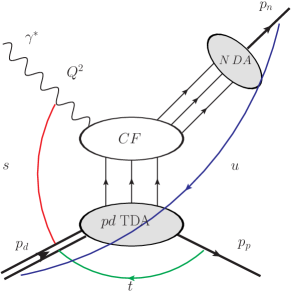
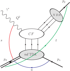
Baryon-to-meson (baryon-to-photon) TDAs occur within the collinear factorized description of a class of hard exclusive reactions with a non-zero baryon number exchange in the cross channel. Prominent examples of such reactions are the backward DVCS and backward hard electroproduction of mesons off nucleons [19, 20] and nucleon–antinucleon annihilation into a lepton pair (or a heavy quarkonium) associated with production of a light meson [21, 22].

The non-local three-quark light-cone operator written above has been used for a long time to define the baryon distribution amplitudes (DAs) through the vacuum to baryon matrix elements: $\langle B(p_{B})\rvert\hat{O}_{\rho\tau\chi}(z_{1},z_{2},z_{3})|0\rangle\,.$ These non-perturbative objects were extensively applied to provide the factorized description of various reactions including the QCD description of the nucleon electromagnetic form factors and heavy quarkonium decay [23, 24, 25]. For a review see e.g. Refs. [26, 27].

Thus, baryon-to-meson (and baryon-to-photon) TDAs share common features both with baryon DAs and with GPDs and encode a conceptually close physical picture. They characterize partonic correlations inside a baryon and give access to the momentum distribution of the baryonic number inside a baryon. Similarly to GPDs, TDAs – after the Fourier transform in the transverse plane – represent valuable information on the transverse location of hadron constituents.

Recent experimental studies [28, 29, 30] brought first evidences in favor of the validity of the reaction mechanism involving nucleon-to-meson TDAs for the description of backward pion or $\omega$-electroproduction at JLab kinematical conditions. The perspective to access baryon-to-meson TDAs experimentally [31, 32, 33, 34] rises a high demand for a consistent exposition of the considerable theoretical progress in the field achieved during the last two decades.

This review presents, in a broad context of applications of the collinear factorization approach in QCD, the physical content of TDAs as well as their application to the description of hadronic structure. We also present an overview of existing phenomenological models of TDAs and their predictions for the kinematical conditions of existing and planned experimental facilities. The results of existing feasibility studies [35, 36] are also reported.

The review is much inspired by the original papers [37, 38, 39, 40, 19, 21, 22, 20, 41] published by the authors and their collaborators during these last 15 years.

2 Collinear factorization framework for hard exclusive reactions

This section is devoted to a brief overview of the main theoretical concepts, which provide the basis for the description of hard exclusive processes in the near-forward kinematics within the collinear factorization framework. These developments began with the analysis of deep inelastic scattering processes and the introduction of the partonic description of inclusive cross sections. Historically, it has contributed a lot to the confidence we now have in QCD as a consistent theory of strong interactions. Following that, we recall the description of electromagnetic form factors at large momentum transfer in terms of hadron distribution amplitudes. We finally sketch the main results of the collinear QCD description of near-forward scattering amplitudes in terms of GPDs and review their basic properties. These concepts will be generalized in the following sections to provide a description of hard exclusive processes in the near-backward kinematics in terms of TDAs.

2.1 Deep inelastic scattering and parton distribution functions

The QCD collinear factorization framework [4, 5] has been primarily developed for inclusive reactions such as deep inelastic scattering (DIS), hadron production in $e^{+}e^{-}$-collisions, lepton pair production in hadron–hadron collisions (Drell–Yan), hadron (or jet) production at large transverse momentum in hadron–hadron collisions.

The collinear factorization theorem for the DIS (see Fig. 1) allows to present the corresponding cross sections as a convolution of perturbatively calculable coefficient functions (CFs) with parton distribution functions (PDFs). Below we consider the case of a pseudoscalar meson target. Within the light-cone gauge ($A^{+}=0$) the corresponding quark PDF is defined as the diagonal hadronic matrix element of the non-local quark–antiquark light-cone operator:

$$q_{\pi}(x,\mu^{2})=\int\frac{dz^{-}}{4\pi}e^{ixp\cdot z}\langle\pi(p)|\bar{\Psi}(-z/2)\gamma^{+}\Psi(z/2)|\pi(p)\rangle\big{|}_{z^{+}=0,\ z_{T}=0}\,.$$ (2.1)

Here $x$ is the Bjorken variable; $z$ is the light cone distance ($z^{2}=0$); $\gamma^{+}\equiv 2\gamma^{\mu}n_{\mu}$, with $n$ being a light cone vector ($n^{2}=0$); and $\mu$ is the factorization scale. Note that since for DIS the factorization occurs at the cross section level, the matrix elements defining PDFs are diagonal. This comes from the fact that an inclusive DIS cross section is represented as the imaginary part of a forward Compton amplitude.

Figure 1: Factorization of DIS : the optical theorem relates the total cross section of DIS ($\gamma^{*}\pi\to X$) to the imaginary part of the forward Compton amplitude ($\gamma^{*}\pi\to\gamma^{*}\pi$).

The collinear factorization framework for DIS was established through the experimental observation of the Bjorken scaling law, which states that PDFs are $Q^{2}$-independent. This scaling law is however violated by a logarithmic $Q^{2}$-dependence inferred from the Dokshitzer–Gribov–Lipatov–Altarelli–Parisi (DGLAP) evolution equations [42, 43, 44].

Similarly to the DIS case, the QCD analysis of exclusive amplitudes will require the existence of a hard scale, usually denoted as $Q^{2}$, which is large enough to prevent higher twist contributions to pollute the analysis of experimental data. The onset of the collinear factorization (often named partonic regime) is usually probed through the observation of the adequacy of the scaling laws for cross-sections or appropriate polarization observables.

2.2 Electromagnetic form factors and distribution amplitudes

A subsequent application of the collinear factorization approach was proposed in [45, 46, 23] for the description of electromagnetic form factors (FFs) of hadrons at large invariant momentum transfer. In the mesonic case, the relevant hadronic matrix element of the light-cone $\bar{\Psi}\Psi$ operator is

$$\langle\pi(p)|\bar{\Psi}(-z/2)\gamma^{+}\Psi(z/2)|0\rangle\,,$$ (2.2)

while in the baryonic case, the relevant matrix element of the three-quark light-cone operator $\Psi\Psi\Psi$ is

$$\langle B(p)|\varepsilon_{c_{1}c_{2}c_{3}}\Psi_{\rho}^{c_{1}}(z_{1})\Psi_{\tau}^{c_{2}}(z_{2})\Psi_{\chi}^{c_{3}}(z_{3})|0\rangle\,.$$ (2.3)

The corresponding hadronic quantities, the distribution amplitudes (DAs), are the Fourier transforms of the matrix elements (2.2), (2.3) decomposed over an appropriate set of the Dirac structures (for a review, see Refs. [24, 26, 27]). The factorization scale dependence of hadron DAs is controlled by the Efremov–Radyushkin–Brodsky–Lepage (ERBL) [47, 45, 46, 48, 23] evolution equations.

Figure 2: Examples of Feynman graphs contributing to the meson (left panel) and baryon (right panel) electromagnetic form factor at the tree level.

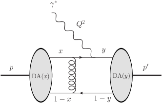
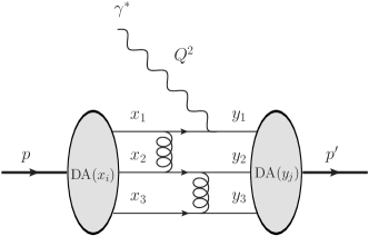
Fig. 2 provides examples of leading order diagrams contributing to the meson and baryon electromagnetic form factor. The scaling law predicted by the QCD collinear factorization framework, namely

$$F_{\pi}(Q)\sim\frac{1}{Q^{2}}\leavevmode\nobreak\ ;\leavevmode\nobreak\ \leavevmode\nobreak\ \leavevmode\nobreak\ F_{1\,N}(Q)\sim\frac{1}{Q^{4}}\,,$$ (2.4)

was a first indication of the success of this approach, as were the successes of the dimensional scaling laws [49, 50] for many fixed angle scattering processes [51].

Further development of the collinear factorization approach, however, revealed subtleties in the application to fixed angle hadronic scattering (for a review, see e.g. Ref. [4]). The importance of the Sudakov suppression of some delicate integration regions was in particular discovered [52], which in turn may help to understand the suppression of endpoint region contributions for meson and baryon form factors [53, 54] (for an alternative point of view, see [55, 56]). Moreover, the absence of pinch singularities, which is a necessary element of the proof of factorization, was shown in [57] for the scattering amplitude for electroproduction processes at fixed angle, putting on a firm ground the collinear factorized framework for various processes.

However, nowadays it is recognized that the hard scattering mechanism alone does not provide a satisfactory description of the existing electromagnetic form factor data up to rather large values of $Q^{2}$. A possible remedy was proposed within the framework based on the light-cone sum rules (LCSRs) (see e.g. Ref. [58] for a review). Within this approach the “soft contributions” into form factors are systematically computed in terms of the same DAs that occur in the collinear factorization framework. The application of the LCSR approach to nucleon form factors is presented in Refs. [59, 60, 61].

2.3 Near-forward exclusive scattering and generalized parton distributions

A significant breakthrough in QCD appeared when it was realized [62, 63, 64, 65, 66] that some exclusive processes, such as the deeply virtual Compton scattering (DVCS)

$$\gamma^{*}(q)+N(p)\to\gamma(q^{\prime})+N(p^{\prime})\,,$$ (2.5)

and hard exclusive meson production (HMP)

$$\gamma^{*}(q)+N(p)\to{\mathcal{M}}(p_{\mathcal{M}})+N(p^{\prime})\,,$$ (2.6)

in the generalized Bjorken limit of large $Q^{2}=-q^{2}$, $W^{2}=(p+q)^{2}$ with fixed $x_{B}=Q^{2}/(2p\cdot q)$, and for a limited range of the invariant momentum transfer $t=(p-p^{\prime})^{2}\sim 0$ proceed via the short-distance scattering on a single parton and may be subject to a collinear factorized description. The condition $t\sim 0$ corresponds to the final state photon (or meson) produced in the nearly forward direction in the $\gamma^{*}N$ center-of-mass system (CMS). Therefore, the corresponding kinematical regime is often referred to as near-forward kinematics.

A much related subject is the discussion of the crossed reaction to the DVCS process (2.5), deep exclusive small invariant mass ($s=(p_{1}+p_{2})^{2}\ll Q^{2}$) hadron pair production:

$$\gamma^{*}(q)+\gamma(q^{\prime})\to H_{1}(p_{1})+H_{2}(p_{2})\,,$$ (2.7)

where collinear factorized description is performed in terms of generalized distribution amplitudes (GDAs) [62, 67] defined as the Fourier transforms of the matrix elements $\langle H_{1}(p_{1})H_{2}(p_{2})|\bar{\Psi}(-z/2)\gamma^{+}\Psi(z/2)|0\rangle$.

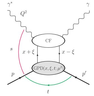
For definiteness here we limit our considerations to the simplest case of DVCS on a pseudoscalar meson target. The corresponding collinear factorization mechanism is presented in Fig. 3. The short-distance process amplitude (CF) involves only longitudinal momenta. It can be systematically computed in the perturbation theory. The DVCS amplitude is presented as a convolution of the corresponding perturbative amplitude with the Fourier transforms of off-diagonal matrix elements of quark (or gluon) light-cone operators [68, 62], named generalized parton distributions (GPDs).

Subsequent developments [6, 64, 66] led to the detailed understanding of this new tool for the study of the physics of confined quarks and gluons and the description of hadron structure. We refer the reader to a collection of excellent reviews [11, 12, 13, 14] existing on this subject. In the remaining part we will quote some crucial features of the near-forward GPD framework. In Sections 3, 4, with appropriate modification, these features will be adapted to the near-backward TDA framework.

In particular, the leading chiral-even twist-$2$ quark GPD of a pseudoscalar meson is defined as the hadronic matrix element of the $\bar{\Psi}\Psi$ operator on the light cone:

$$H^{q}_{\pi}(x,\xi,t,\mu^{2})=\int\frac{dz^{-}}{4\pi}e^{ixP\cdot z}\langle\pi(p^{\prime})|\bar{\Psi}(-z/2)\gamma^{+}\Psi(z/2)|\pi(p)\rangle\big{|}_{z^{+}=0,\;{z_{T}}=0}\,,$$ (2.8)

where $P\equiv\frac{p+p^{\prime}}{2}$; $\Delta\equiv p^{\prime}-p$; $x$ is the light cone momentum fraction variable, $\xi=-\frac{\Delta^{+}}{2P^{+}}$, the so-called skewness variable, characterizes the longitudinal momentum transfer between the initial and final hadron states, $t=\Delta^{2}$ is the invariant squared momentum transfer and $\mu$ is the factorization scale. In the forward limit $\xi=0$, $t=0$ the GPD (2.8) reduces to the forward PDF (2.1):

$$H^{q}_{\pi}(x,\xi=0,t=0,\mu^{2})=q_{\pi}(x,\mu^{2}).$$ (2.9)

Figure 3: Collinear factorization mechanism for DVCS.

The GPDs possess the restricted $[-1,\,1]$ support in the longitudinal momentum-fraction variable $x$. Their partonic interpretation in the momentum space leads to the definition of three distinct regions corresponding to different directions of the longitudinal momentum flows:

• When $x>\xi$, both momentum fractions $x+\xi$ and $x-\xi$ are positive and GPDs describe the emission and reabsorption of a quark.

• When $|x|\leq\xi$, the momentum fraction $x-\xi$ is interpreted as belonging to an antiquark with momentum fraction $\xi-x$, and GPDs describe the emission of a quark–antiquark pair from the initial hadron.

• When $x<-\xi$, both momentum fractions $x+\xi$ and $x-\xi$ are negative and are interpreted as belonging to antiquarks with momentum fraction $\xi-x$ and $-\xi-x$, GPDs describing then the emission and reabsorption of an antiquark.

The scale evolution of hadronic matrix elements of light-cone operators turns to be firstly a property of the operators in question. Since the quark–antiquark $\bar{\Psi}\gamma^{+}\Psi$ operator occurring in the definition of quark GPDs is the same as that defining PDFs and mesonic DAs, the evolution equations for GPDs are much related to the DGLAP evolution equations for PDFs and the ERBL evolution of DAs [62]. In fact, the GPD evolution in the outer support regions $x>\xi$ and $x<-\xi$ (often called the DGLAP regions) is governed by the DGLAP-type equations, while in the inner support region $|x|\leq\xi$ (referred to as the ERBL region), the evolution equations turn to be of the ERBL-type.

Among the various GPD properties a special role is attributed to the so-called polynomiality property of the Mellin moments of GPDs in the momentum-fraction variable $x$. This highly non-trivial constraint is a direct consequence of the underlying Lorentz invariance. Indeed, integrating over $x$ the matrix elements of bilocal operators removes all reference to a light-cone axis defined by the vector $n$ and provides matrix elements of local operators. The $N$th Mellin moment of a GPD turns to be a polynomial of order (at most) $N+1$ in the skewness variable $\xi$. The coefficients at powers of $\xi$ can be expressed through the form factors of the local twist-$2$ operators:

$$\widehat{O}^{\mu\mu_{1}...\mu_{N}}(0)=\bar{\Psi}(0)\gamma^{\mu}i\overleftrightarrow{D}^{\mu_{1}}...\,i\overleftrightarrow{D}^{\mu_{N}}\Psi(0),$$ (2.10)

where $\overleftrightarrow{D}^{\mu}=\overleftrightarrow{\partial}^{\mu}-igA^{a\,\mu}t^{a}$ is the covariant derivative. Here $t^{a}=\frac{\lambda^{a}}{2}$ with $\lambda^{a}$, $a=1,\ldots,8$ being the Gell-Mann matrices; $\overleftrightarrow{\partial}^{\mu}\equiv\frac{1}{2}\left(\overrightarrow{\partial}^{\mu}-\overleftarrow{\partial}^{\mu}\right)$.

The polynomiality property brings one of the most important practical application of the GPD formalism. The study of the first Mellin moment of quark (gluon) GPDs provides access to the hadronic matrix elements of the quark (respectively gluon) part of the QCD energy momentum tensor. This allows to address the origin of hadron’s spin [6, 69] and build up a comprehensible picture of the “mechanical properties” of hadrons [70, 71].

A convenient way to implement both the support and the polynomiality properties of GPDs consists in expressing them in terms of more fundamental quantities, the double distributions (DDs) [63, 72, 73] (also called spectral densities in [62]). The basic idea is to present the relevant hadronic matrix elements as the Fourier-transform with respect to two independent scalars $P\cdot z$ and $\Delta\cdot z$. The corresponding double distribution $f(\alpha,\beta,t)$ has the restricted support in the spectral variables $(\alpha,\beta)$, which is the rhombus $\Omega:\;|\alpha|+|\beta|\leq 1$. The double distribution representation of GPDs highlights the hybrid nature of GPDs that combine the properties of forward parton densities in the $\xi\to 0$ limit and those of distribution densities in the $\xi\to 1$ limit.

In the original formulation of DD representation, in order to satisfy the polynomiality condition in its complete form, the spectral part must be supplemented with the so-called $D$-term [74]:

$$H^{q}(x,\xi,t)=\int_{\Omega}d\alpha d\beta\,\delta(x-\beta-\xi\alpha)f(\beta,\alpha,t)+\theta(\xi-|x|)D\left(\frac{x}{\xi},t\right).$$ (2.11)

The $D$-term produces the highest possible power of $\xi$ ($\xi^{N+1}$) of the $N$th ($N$ -odd) Mellin moments of the $C$-even GPD. In fact, as pointed out in Ref. [75], the DD representation turns to be defined up to a “gauge transformation”. By altering the admittable analytic properties of the spectral densities [76] one can also obtain representations [77] with a $D$-term implemented into the spectral density. The double distribution of GPDs was extensively employed to provide the framework for various phenomenological models for GPDs.

The physical contents of GPDs became more transparent within the impact parameter space interpretation proposed in [8, 9, 10]. The basic idea is to employ the mixed representation of GPDs Fourier transformed from transverse momentum to transverse position, referred as the “impact parameter”. This allows to perform hadron tomography in the transverse plane and highlight the new physical information encoded in GPDs with respect to forward PDFs.

The transition to the impact parameter implies introducing hadron states of definite light cone momentum and definite position ${\mathbf{b}}$ in the transverse plane $|p^{+},{\mathbf{b}}\rangle$ and consideration of transverse position dependent quark–antiquark operator. The Fourier transform of GPDs is performed with respect to the transverse part ${\mathbf{D}}$ of the $4$-vector $D=\frac{p^{\prime}}{1-\xi}-\frac{p}{1+\xi}$. It is related to the Mandelstam invariant $t$ by

$$t=t_{0}-(1-\xi^{2}){\mathbf{D}}^{2},$$ (2.12)

where $t_{0}=\frac{-4\xi^{2}m^{2}}{1-\xi^{2}}$ is the largest possible value of $t$. In the DVCS case, $t=t_{0}$ corresponds to the final state photon produced exactly in the forward direction.

For the case of the spin-$0$ target the resulting impact parameter representation of GPDs reads [10]:

$$\int\frac{d^{2}{\mathbf{D}}}{4\pi^{2}}e^{-i({\bf D}\cdot{\bf b})}H(x,\xi,t)={\mathcal{N}}\frac{1+\xi^{2}}{(1-\xi^{2})^{5/2}}\langle p^{\prime+},-\frac{\xi{\mathbf{b}}}{1-\xi}|\widehat{O}({\mathbf{b}})|p^{+},\frac{\xi{\mathbf{b}}}{1+\xi}\rangle\,,$$ (2.13)

where ${\mathcal{N}}$ is a normalization factor and the transverse position dependent non-local quark–antiquark operator is

$$\widehat{O}({\mathbf{b}})=\int\frac{dz^{-}}{4\pi}e^{ixP^{+}z^{-}}\bar{\Psi}(0,-z^{-}/2,{\mathbf{b}})\gamma^{+}\Psi(0,z^{-}/2,{\mathbf{b}})\,.$$ (2.14)

A similar impact parameter representation was established in [78] for the cross-channel counterparts of GPDs — GDAs of hadronic states with meson quantum numbers.

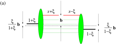
The interpretation of the GPD impact parameter representation (2.14) is illustrated in Fig. 4 separately for the DGLAP and the ERBL regions. Depending on the $x$-range the relevant matrix element describes different processes.

• In the DGLAP region $x>\xi$ (or $x<-\xi$) the emission and subsequent reabsorption of a quark (or antiquark) at transverse position ${\mathbf{b}}$.

• In the ERBL region $|x|\leq\xi$ the emission of a quark–antiquark pair at transverse position ${\mathbf{b}}$.

The non-zero skewness results in $\xi$-dependent transverse shifts of centers of incoming and outgoing particles. This reflects the fact that GPDs are more complicated objects than PDFs which admit a simple probability densities interpretation.

Figure 4: The impact parameter space representation of GPDs: (a) DGLAP region of GPDs with $x\in[\xi,1]$, (b) ERBL region of GPDs with $x\in[-\xi,\xi]$. [Reprinted Figure 12 from Ref. [12]. Copyright (2003) by Elsevier.]

3 Probing dynamics of the near-backward hard exclusive meson electroproduction

In this section we present the near-backward kinematical regime for the reaction of hard exclusive meson electroproduction off a nucleon. Following that, we discuss the present status of the collinear factorization theorem providing a description of this reaction in terms of nucleon-to-meson TDAs and nucleon DAs in the generalized Bjorken limit. We also shortly discuss the alternative description of hard processes within the Regge theory approach. We conclude this section with a summary of the color transparency effects to understand which further experimental data are of crucial importance to test the onset of the TDA description.

3.1 Light-cone kinematics for the near-backward regime

Let us consider hard exclusive meson electroproduction off a nucleon

$$e(k,s_{e})+N(p_{N},s_{N})\to\left(\gamma^{*}(q,\lambda_{\gamma})+N(p_{N},s_{N})\right)+e(k^{\prime},s^{\prime}_{e})\to e(k^{\prime},s^{\prime}_{e})+N(p^{\prime}_{N},s^{\prime}_{N})+{\mathcal{M}}(p_{\mathcal{M}})$$ (3.1)

in the generalized Bjorken limit within the near-backward kinematics regime. For the moment we do not specify the nature of the final state meson (this can be a light pseudoscalar $\pi$, $\eta$, $\eta^{\prime}$ or a light vector $\rho$, $\omega$)

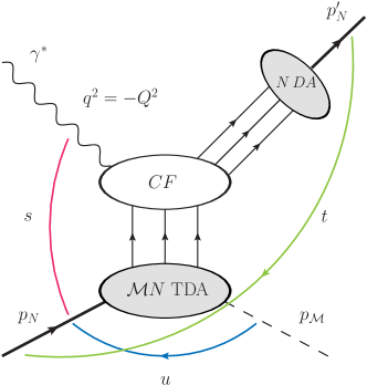
The relevant kinematical quantities for the hard subprocess

$$\gamma^{*}(q,\lambda_{\gamma})+N(p_{N},s_{N})\to N(p^{\prime}_{N},s^{\prime}_{N})+{\cal{M}}(p_{\cal{M}})$$ (3.2)

of the reaction (3.1) are presented in Fig. 5. We employ the usual notations for the photon virtuality, the $\gamma^{*}N$ center-of-mass energy $W$, and the Bjorken variable $x_{B}$

$$Q^{2}=-q^{2};\ \ W^{2}=(p_{N}+q)^{2};\ \ x_{B}=\frac{Q^{2}}{2p_{N}\cdot q},$$ (3.3)

and introduce the standard Mandelstam variables

$$s\equiv W^{2};\ \ t=(p^{\prime}_{N}-p_{N})^{2};\ \ u=(p_{\mathcal{M}}-p_{N})^{2}.$$ (3.4)

The Mandelstam variables (3.4) satisfy

$$s+t+u=-Q^{2}+2m_{N}^{2}+m_{\mathcal{M}}^{2}\,,$$ (3.5)

where $m_{N}$ and $m_{\mathcal{M}}$ denote respectively the nucleon and the meson masses.

Figure 5: Kinematical quantities and the collinear factorization mechanism for $\gamma^{*}N\to N{\mathcal{M}}$ in the near-backward kinematical regime (large $Q^{2}$, $W$; fixed $x_{B}$; $|u|\sim 0$). The lower blob, denoted ${\mathcal{M}}N$ TDA, depicts the nucleon-to-meson $\mathcal{M}$ transition distribution amplitude; $N$ DA blob depicts the nucleon distribution amplitude; $CF$ denotes the hard subprocess amplitude (coefficient function).

Within the generalized Bjorken limit, the near-backward kinematics corresponds to large $Q^{2}$ and $W^{2}$ with fixed $x_{B}$ and small invariant momentum transfer between the final meson and the initial nucleon:

$$|u|=|(p_{\mathcal{M}}-p_{N})^{2}|\ll Q^{2},\,W^{2}.$$ (3.6)

This corresponds to the final state meson produced in a nearly backward direction in the $\gamma^{*}N$ center-of-mass-system (CMS). Note that the condition (3.5) together with (3.6) implies that in the near-backward kinematics the invariant momentum transfer $t$ between the initial and final state nucleons is large (by the absolute value) and negative.

The near-backward kinematical regime can be seen as being complementary to the more familiar near-forward kinematics with large $Q^{2}$ and $W^{2}$, fixed $x_{B}$ and small invariant momentum transfer $|t|$ between the final and initial nucleons:

$$|t|=|(p^{\prime}_{N}-p_{N})^{2}|\ll Q^{2},\,W^{2}\,,$$ (3.7)

where the collinear factorization providing a description in terms of GPDs is at work. This kinematical regime corresponds to the final state nucleon produced in the near-backward direction in the $\gamma^{*}N$ CMS and hence the final state meson produced in the near-forward direction.

A common procedure to address the reaction (3.1) in both near-forward and near-backward kinematics consists in the introduction of light-cone coordinates. The $z$-axis is naturally chosen along the colliding virtual photon and nucleon. We introduce the light-cone vectors $p$ and $n$:

$$p^{2}=n^{2}=0;\ \ 2p\cdot n=1.$$ (3.8)

Then for an arbitrary four-vector $l^{\mu}$ we introduce the Sudakov decomposition

$$l^{\mu}=l^{+}p^{\mu}+l^{-}n^{\mu}+l^{\mu}_{T};\ \ \ l^{2}=l^{+}l^{-}+l^{2}_{T},$$ (3.9)

where $l^{+}=2(n\cdot l)$; $l^{-}=2(p\cdot l)$; and the $T$ subscript is adopted for the transverse part of a four-vector $l^{\mu}$, which satisfies $(p\cdot l_{T})=(n\cdot l_{T})=0$. In some cases we also use boldface for the Euclidian two-dimensional transverse components of vectors ${\mathbf{l}}=(l^{1},l^{2})$: $l^{2}=l^{+}l^{-}-{\mathbf{l}}^{2}.$

We employ the notation $\Delta$ for the momentum transfer between the final state meson and the initial state nucleon ($u$-channel momentum transfer):

$$\Delta\equiv p_{\mathcal{M}}-p_{N};\ \ \ \Delta^{2}=u;$$ (3.10)

and define the average nucleon–meson momentum $P$ and mass $\bar{m}_{{\mathcal{M}}N}$:

$$P\equiv\frac{1}{2}\left(p_{N}+p_{\mathcal{M}}\right);\ \ \ P^{2}=\bar{m}^{2}_{{\mathcal{M}}N}=\frac{1}{2}\left(m_{N}^{2}+{m_{\mathcal{M}}^{2}}\right)-\frac{\Delta^{2}}{4}.$$ (3.11)

Keeping the first-order corrections in squared masses and in the square of the transverse momentum transfer $\Delta_{T}^{2}$, we establish the following Sudakov decomposition for the momenta of the reaction (3.1) in the near-backward kinematical regime (cf. Ref. [37]):

$$p_{N}=(1+\xi)p+\frac{m_{N}^{2}}{1+\xi}n\,;$$

$$p_{\mathcal{M}}=(1-\xi)p+\frac{m^{2}_{\mathcal{M}}-\Delta_{T}^{2}}{1-\xi}n+\Delta_{T}\,;$$

$${}\Delta=-2\xi p+\Bigl{[}\frac{m^{2}_{\mathcal{M}}-\Delta_{T}^{2}}{1-\xi}-\frac{m_{N}^{2}}{1+\xi}\Bigr{]}n+\Delta_{T}\,;$$

$$P=p+\frac{1}{2}\Bigl{[}\frac{m_{N}^{2}}{1+\xi}+\frac{m^{2}_{\mathcal{M}}-\Delta_{T}^{2}}{1-\xi}\Bigr{]}n+\frac{1}{2}\Delta_{T};$$ (3.12)

$${}p^{\prime}_{N}\simeq-2\xi\frac{(\Delta_{T}^{2}-m_{N}^{2})}{Q^{2}}p+\left[\frac{Q^{2}}{2\xi\Bigl{(}1+\frac{(\Delta_{T}^{2}-m_{N}^{2})}{Q^{2}}\Bigr{)}}-\frac{m^{2}_{\mathcal{M}}-\Delta_{T}^{2}}{1-\xi}+\frac{m_{N}^{2}}{1+\xi}\right]n-\Delta_{T};$$

$$q\simeq-2\xi\Bigl{(}1+\frac{(\Delta_{T}^{2}-m_{N}^{2})}{Q^{2}}\Bigr{)}p+\frac{Q^{2}}{2\xi\Bigl{(}1+\frac{(\Delta_{T}^{2}-m_{N}^{2})}{Q^{2}}\Bigr{)}}n\,.$$ (3.13)

The square of the transverse momentum transfer $\Delta_{T}^{2}$ is defined below in Eq. (3.16) and $\xi$ stands for the $u$-channel skewness variable introduced with respect to the $u$-channel momentum transfer

$$\xi=-\frac{(p_{\mathcal{M}}-p_{N})\cdot n}{(p_{\mathcal{M}}+p_{N})\cdot n}.$$ (3.14)

For the leading twist accuracy calculations we employ the approximate expression for the skewness variable $\xi$ (3.14) neglecting order-of-mass and $\Delta_{T}^{2}$ corrections

$$\xi\simeq\frac{x_{B}}{2-x_{B}}=\frac{Q^{2}}{Q^{2}+2W^{2}}+{\mathcal{O}}(1/Q^{2}).$$ (3.15)

The $u$-channel transverse momentum transfer squared is expressed as

$$\Delta_{T}^{2}=\frac{1-\xi}{1+\xi}\left(\Delta^{2}-2\xi\left[\frac{m_{N}^{2}}{1+\xi}-\frac{m_{\mathcal{M}}^{2}}{1-\xi}\right]\right).$$ (3.16)

We introduce $u_{0}$ corresponding to $\Delta_{T}^{2}=0$:

$$u_{0}=-\frac{2\xi\left(m_{\mathcal{M}}^{2}(1+\xi)-m_{N}^{2}(1-\xi)\right)}{1-\xi^{2}}.$$ (3.17)

It is the maximal possible value of $u$ for given $\xi$. For $\Delta_{T}^{2}=0$ ($u=u_{0}$) the meson is produced exactly in the backward direction in the $\gamma^{*}N$ CMS ($\theta_{\mathcal{M}}^{*}=\pi$). Note that, for small meson masses, $u_{0}$ is positive for most values of $\xi$.

In the initial state nucleon rest frame, which corresponds to the laboratory (LAB) frame of a fixed target experiment, the light-cone vectors $p$ and $n$ read

$$p\Big{|}_{\rm LAB}=\frac{m_{N}}{2(1+\xi)}\{1,0,0,-1\};\ \ \ n\Big{|}_{\rm LAB}=\frac{1+\xi}{2m_{N}}\{1,0,0,1\}.$$ (3.18)

With the help of the appropriate boost we establish the expressions for the light-cone vectors in the $\gamma^{*}N$ CMS:

$$p\Big{|}_{\gamma^{*}N\,{\rm CMS}}=\alpha(W^{2},\,Q^{2},\,m_{N}^{2})\{1,0,0,-1\};\ \ \ n\Big{|}_{\gamma^{*}N\,{\rm CMS}}=\frac{1}{4\alpha(W^{2},\,Q^{2},\,m_{N}^{2})}\{1,0,0,1\},$$ (3.19)

with

$$\alpha(W^{2},\,Q^{2},\,m_{N}^{2})=\frac{W^{2}+Q^{2}+m_{N}^{2}+\Lambda\left(W^{2},-Q^{2},m_{N}^{2}\right)}{4(1+\xi)W},$$ (3.20)

where $\Lambda$ is the usual Mandelstam function

$$\Lambda(x,y,z)=\sqrt{x^{2}+y^{2}+z^{2}-2xy-2xz-2yz}\,.$$ (3.21)

The $\mathcal{M}$-meson scattering angle in the $\gamma^{*}N$ CMS for the near-backward kinematical regime can be expressed as

$$\cos\theta_{\mathcal{M}}^{*}=\frac{-4(1-\xi)^{2}\alpha^{2}(W^{2},\,Q^{2},\,m_{N}^{2})+{m^{2}_{\mathcal{M}}-\Delta_{T}^{2}}}{\sqrt{\left(-4(1-\xi)^{2}\alpha^{2}(W^{2},\,Q^{2},\,m_{N}^{2})+m^{2}_{\mathcal{M}}-\Delta_{T}^{2}\right)^{2}-16\alpha^{2}(W^{2},\,Q^{2},\,m_{N}^{2})(1-\xi)^{2}\Delta_{T}^{2}}}\,\,,$$ (3.22)

where $\alpha(W^{2},\,Q^{2},\,m_{N}^{2})$ is given by (3.20). One may check that for $\Delta_{T}^{2}=0$ indeed $\cos\theta_{\mathcal{M}}^{*}=-1$, corresponding to a meson $\mathcal{M}$ produced exactly in the backward direction in the $\gamma^{*}N$ CMS.

3.2 Status of the collinear factorization theorem

The research program aiming at the study of nucleon-to-meson TDAs in hard exclusive backward meson electroproduction reactions (and in the cross-channel counterpart reactions) is generally analogous to the extraction of GPDs from DVCS and hard exclusive near-forward meson electroproduction.

The possibility to access nucleon-to-meson TDAs in hard exclusive backward meson electroproduction reactions is based on the collinear factorization theorem that is similar to the familiar factorization theorems for the near-forward hard exclusive electroproduction of mesons [65] and DVCS [79]. This collinear factorization theorem was first conjectured in Refs. [16, 80], although never proven consistently.

There are several approaches for providing proofs for collinear factorization theorems (see e.g. Sec.5.1 of [12] and Ref. [81] for a review).

• The approach employed by J. Collins et al. [65, 79] and by X.-D. Ji and J. Osborne [82] relies on the general properties of the Feynman diagrams and makes use of the theoretical tools developed by S. Libby, G. Sterman and J. Collins [83, 84, 85, 86] (for a detailed description see Refs. [87, 5]). The Coleman–Norton theorem [88] allows to locate the regions of the loop momentum space giving rise to the leading asymptotic behavior of the relevant Feynman diagrams.

• The alternative approach of A. Radyushkin [66] addresses the spectral properties of the Feynman diagrams using the $\alpha$-representation technique [89, 90].

• A systematic framework to study QCD factorization is provided by the effective theory approach [91], the so-called Soft Collinear Effective Theory (SCET). This latter framework provides a consistent description of both hard and soft spectator scattering mechanisms and was in particular applied to the description of the nucleon form factor [92] and to the description of the wide-angle Compton scattering [93].

In this section, mainly following Refs. [65, 79, 94], we discuss some of the essential steps in the construction of a factorization theorem for hard exclusive backward meson electroproduction. Let us thus consider the reaction (3.1). In the limit

$$-q^{2}\equiv Q^{2}\to\infty\ \ \text{with fixed}\ \ \frac{Q^{2}}{W^{2}}\ \ \text{and small}\ \ |u|=|(p_{\mathcal{M}}-p_{N})^{2}|\,,$$ (3.23)

the scattering amplitude of the hard subprocess of (3.1)

$$\gamma^{*}(q)+N(p_{N})\to{\mathcal{M}}(p_{\mathcal{M}})+N(p^{\prime}_{N}).$$ (3.24)

for a transversely polarized virtual photon, up to $1/Q$ suppressed corrections, reads [37]:

$${\mathcal{A}}(\gamma^{*}_{T}N\to{\mathcal{M}}N)\simeq\frac{1}{Q^{3}}\int_{-1+\xi}^{1+\xi}dx_{1}dx_{2}dx_{3}\delta(\sum_{k=1}^{3}x_{k}-2\xi)\int_{0}^{1}dy_{1}dy_{2}dy_{3}\delta(\sum_{l=1}^{3}y_{l}-1){}$$

$$\ T^{ij}(x_{1,2,3},\,\xi,\,y_{1,2,3};\,\mu^{2})F^{i}(x_{1,2,3},\,\xi,\,u;\,\mu^{2})\,\Phi^{j}(y_{1,2,3};\,\mu^{2}).$$ (3.25)

Here $F^{i}$ stands for the matrix element of the light-cone $3$-quark operator of the relevant flavor contents between the initial nucleon and final meson states expressed through nucleon-to-meson TDAs; $\Phi^{j}$ denotes the distribution amplitude of the final nucleon state; $T^{ij}$ is the hard part of the corresponding amplitude. $x_{1,2,3}$ stand for the momentum fractions of quarks coming from the initial nucleon; $y_{1,2,3}$ are the momentum fractions of quarks of the final state nucleon. The skewness variable $\xi$ (3.14) is defined with respect to the longitudinal momentum transfer between the initial nucleon and the final meson. The factorization scale $\mu$ is supposed to be of order $Q$. The factorization scale dependence of nucleon-to-meson TDAs and nucleon DAs is given by the appropriate evolution equations. We adopt a reference frame in which the external momenta of (3.24) have small transverse components of the order $\sqrt{u_{0}-u}\sim{\mathcal{O}}(m_{N})$ (see Sec. 3.1 for the details of our kinematics conventions).

In order to employ the power-counting technique of Refs. [65, 79] that allows to identify the leading power contributions to the amplitude of (3.24) we establish the following counting rules for the relevant momenta denoted $(l^{+},l^{-},l_{\bot})$:

$$\text{hard part}\ \ H:\;\left({\mathcal{O}}(Q),\,{\mathcal{O}}(Q),\,{\mathcal{O}}(m_{N})\right);{}$$

$$\text{incoming nucleon}:\ \ \left({\mathcal{O}}(Q),\,{\mathcal{O}}(m_{N}^{2}/Q),\,{\mathcal{O}}(m_{N})\right);{}$$

$$\text{outgoing meson}:\ \ \left({\mathcal{O}}(Q),\,{\mathcal{O}}(m_{\mathcal{M}}^{2}/Q),\,{\mathcal{O}}(m_{\mathcal{M}})\right);{}$$

$$\text{outgoing nucleon}:\ \ \left(\,{\mathcal{O}}(m_{N}^{2}/Q),{\mathcal{O}}(Q),\,{\mathcal{O}}(m_{N})\right);{}$$

$$\text{soft part}\ \ S:\text{all components of momenta small compared to}\;Q.$$ (3.26)

Figure 6: Reduced graph for the factorized description of hard exclusive backward meson electroproduction. Black dots depict arbitrary number of additional collinear gluon lines with suitable longitudinal polarization.

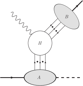
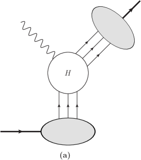
The factorization formula (3.25) corresponds to the contribution of the reduced graph depicted in Fig. 6. The lines of the subgraph $A$ are collinear to the incoming nucleon and outgoing meson; the lines of the subgraph $B$ are collinear to the outgoing nucleon, the lines of the hard subgraph $H$ have large components in both light-cone directions. In addition to the quark lines depicted in Fig. 6 there might be an arbitrary number of collinear gluons with polarization along the plus-direction connecting the subgraphs $A$ and $H$ and of collinear gluons with polarization along the minus-direction connecting the subgraphs $B$ and $H$.

Obviously, this graph corresponds to the textbook hard scattering mechanism proposed a long time ago to provide the leading power behavior within the pQCD description of the nucleon electromagnetic form factor [46, 24] (see Fig. 9 (a)).

Figure 7: General reduced graph potentially contributing to the leading asymptotic regime for hard exclusive backward meson electroproduction. The soft subgraph $S$ is connected to the collinear subgraphs $A$ and $B$ by an arbitrary number of only gluon lines. According to the power counting formula (3.27) this graph contributes to the leading asymptotic behavior (3.28). Graphs with extra lines connecting the $S$-subgraph to the hard part $H$ do not contribute to the leading asymptotic behavior due to $1/Q$-suppression.

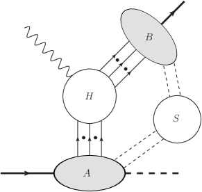
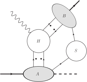
The graph depicted in Fig. 6 is a particular example of a more general class of reduced graphs (see Fig. 7) for the backward reaction (3.24) that may include an additional soft subgraph $S$ connected to $A$, $B$ (and $H$) by an arbitrary number of soft lines depicted by dashed lines.

The power-counting formula that determines the $Q^{p(\pi)}$ behavior of a particular reduced graph takes the same form as in [65]:

$$p(\pi)=3-n(H)-\text{No. (quark lines from}\;S\;\text{to}\;A,\,B\text{)}{}$$

$$-3\cdot\text{No. (quark lines from}\;S\;\text{to}\;H\text{)}-2\cdot\text{No. (gluons lines from}\;S\;\text{to}\;H\text{)},$$ (3.27)

where $n(H)$ is the number of collinear quarks and transversely polarized gluons attached to the hard subgraph.

According to the power counting formula (3.27), the reduced graph depicted in Fig. 6 corresponds to the leading asymptotic behavior

$$Q^{p(\pi)}=Q^{-3}.$$ (3.28)

More generally, the leading power behavior is provided by the graphs depicted in Fig. 7 with soft subgraphs $S$ connected to the collinear subgraphs $A$ and $B$ by an arbitrary number of only gluon lines.

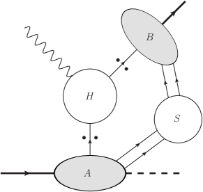
Another class of potentially leading regions corresponds to the soft rescattering mechanism graphs with only one (or two) quark lines entering the hard subgraph with the remaining quark lines connecting $A$ and $B$ through the soft subgraph $S$. There also could be an arbitrary number of gluons connecting $A$ and $B$ to $S$. The power counting formula (3.27) provides the same power-like behavior (3.28) An example of such reduced graphs is depicted in Fig. 8.

Figure 8: Examples of graphs corresponding to the soft rescattering mechanism for the backward reaction (3.24).

Further steps in proving the collinear factorization theorem are:

• Proving the suppression of the contributions of the soft rescattering mechanism graphs in Fig. 8 and the dominance of the transverse polarization of the virtual photon.

• Proving the effective suppression of the soft gluon subgraphs in the contributions of generic reduced graphs in Fig. 7. This provides the “color neutrality” of the final state nucleon and ensures actual dominance of the hard reaction mechanism graph depicted in Fig. 6.

• Implementing the gauge invariance that allows to sum the contributions of collinear gluons polarized along the $+$-direction connecting $A$ and $H$ (respectively collinear gluons polarized along the $-$-direction connecting $B$ and $H$) into the Wilson lines (4.2) that appear in the gauge invariant three-local light-cone operators entering into the definition of nucleon-to-meson TDAs (nucleon DAs), see Sec. 4.1.

• To obtain the final form of the factorization theorem (3.25) the hard subgraph $H$ has to be expanded in the small components of its external momenta:

  $$\int d^{4}l\,d^{4}k\ A(l)B(k)H(l,k)\simeq\int dl^{+}dk^{-}H(l,k)\Big{|}_{{l^{-}=k^{+}=0\atop l_{\bot}=k_{\bot}=0}}\int dl^{-}d^{2}l_{\bot}A(l)\int dk^{+}d^{2}k_{\bot}B(k).$$ (3.29)

  The explicit expressions for the leading order hard scattering amplitudes is presented in Sec. 6.

• Presenting the collinear subgraphs $A(l)$ and $B(k)$ as the Fourier transforms of hadronic matrix elements of position space operators results in the familiar light-cone operator definition of nucleon-to-meson TDAs and nucleon DAs.

• The factorization scale $\mu$ dependence of nucleon-to-meson TDAs is governed by a generalization of the DGLAP and ERBL evolution equations, see Sec. 4.8.

One of the most non-trivial steps in proving the factorization theorem turns to be the demonstration of the suppression of the contributions of the soft rescattering mechanism and the dominance of a particular polarization of the virtual photon.

For the case of near-forward deeply virtual meson production [65] the corresponding proof was based on rather non-trivial arguments [95, 96, 97]. The essential clause is the observation that the final state meson is produced from a small size $q\bar{q}$ configuration created in the hard scattering. Therefore, the soft interactions happen only in the final state, and not in the initial state. The possibility of a proper generalization of these arguments for the case of a three-quark intermediate configuration still remains an open question.

Another perspective on the soft contributions corresponding to graphs in Fig. 8 consists in treating them as the so-called endpoint singularities. Indeed, within the momentum integrals in the factorization formula (3.25) such configurations correspond to the cross-over trajectories $x_{k}=0$, separating the ERBL-like and the DGLAP-like support regions (see Sec. 4.3) of nucleon-to-meson TDAs $F^{i}(x_{1,2,3},\,\xi,\,u)$, and to the endpoint region $y_{l}=0$ of nucleon DAs $\Phi^{j}(y_{1,2,3})$.

The issue of the potential end point singularities has been rather controversial in the literature. In particular, in context of the QCD description of the nucleon electromagnetic form factor the importance of this type of contributions was first highlighted in [98, 99, 100]. In Ref. [46] these arguments were parried by the possible strong suppression of such contributions at large-$Q^{2}$ due to the Sudakov-type all-order resummation of corresponding non-renormalization group logarithms. A detailed study employing the technique originally developed for the case of the pion form factor [53] is presented in Ref. [101], see also the discussion in [102].

Figure 9: (a) Reduced diagram for hard scattering mechanism for nucleon e.m. form factor; (b) reduced diagram for soft rescattering mechanism for nucleon e.m. form factor.

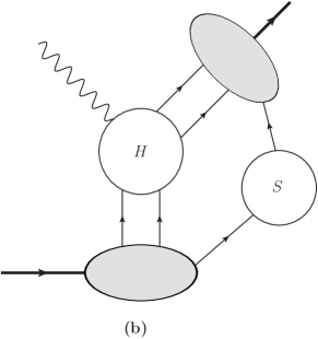
However, the present day experimental studies [103, 104, 105] give evidences that in the region of moderate $Q^{2}\simeq 2.5\text{--}10\leavevmode\nobreak\ \mathrm{GeV}^{2}$ the factorization approach based on the hard scattering mechanism (see Fig. 9(a)) cannot provide a description of some part of existing experimental data. In particular, at this kinematical regime the form factor ratio $F_{2}/F_{1}$ does not follow the asymptotic $Q^{2}F_{2}/F_{1}\sim{\rm const}$ behavior suggested by the pQCD description based solely on the hard scattering mechanism.

This motivated the possible explanations relying on the soft rescattering mechanism, Fig. 9(b). A detailed study of the soft rescattering mechanism for the nucleon form factor within the SCET approach is presented in Refs. [92, 106]. It suggests a large contribution from the soft rescattering mechanism in the region of moderate $Q^{2}$ and brings essential end point singularities that may result in the breakup of the collinear factorization for the FF $F_{1}$

The existing phenomenological approaches based on the QCD-motivated models of hadronic wave functions [107, 108, 109], QCD sum rules [110, 111] and light-cone sum rules [60, 112] provide additional evidences in favor of the relevance of the soft-spectator mechanism for a realistic description of some scattering amplitudes at moderate $Q^{2}$. The generalization of these arguments and the quantitative estimate of the soft spectator mechanism for the reaction (3.24) and possible implications for the collinear factorization breakup at the moment remain open issues.

The issue of collinear factorization breaking should not be confused with the issue of using asymptotic forms of distribution amplitudes. In various phenomenological applications it was noticed that the use of the simple asymptotic DAs usually leads to a rather small contribution into the amplitudes of hard exclusive reactions. A possible way out was suggested by V. Chernyak and A. Zhitnitsky [24]. It consists in using DAs that differ considerably from the asymptotic form and are mostly concentrated near the end points. Effectively, this can be seen as a way to partially take into account the contribution of the soft spectator mechanism and greatly improves the description of the data. The regularization of the potential end point singularities then requires further theoretical efforts (see e.g. the discussion on the pQCD description of $\gamma\gamma^{*}\to\pi^{0}$ form factors in Ref. [113]).

Obviously, the rigorous proof of the collinear factorization theorem for hard exclusive backward meson electroproduction (3.24) and a careful analysis of possible alternative reaction mechanisms are important issues to put the TDA formalism on a firm ground. However, given the considerable technical difficulties in proving the collinear factorization theorems and the still controversial status of the validity of the collinear factorized description even for much simpler hard exclusive reactions at intermediate values of $Q^{2}$, it turns extremely important to simultaneously look for the experimental evidences of the possible early onset of factorization regime for the reaction (3.24). These include

• the characteristic $1/Q^{8}$ scaling behavior of the transverse cross section $\frac{d^{2}\sigma_{T}}{d\Omega_{\mathcal{M}}}$, see Sec. LABEL:SubSec_Bkw_CS;

• the dominance of the transverse cross section $\sigma_{T}$;

• the constant scaling behavior of the cross section ratio $Q^{2}\sigma_{L}/\sigma_{T}$.

It is also worth mentioning that following the analogy with the collinear factorized description of the time-like Compton process proposed in Refs. [114, 115], a version of the collinear factorization theorem (3.25) can be formulated in appropriate kinematical regime for the cross channel counterparts of the reaction (3.24), see Sec. LABEL:SubSec_Cross_Ch_Excl_R. These include nucleon–antinucleon annihilation into a highly virtual lepton pair (or a heavy quarkonium) in association with a light meson $\mathcal{M}$:

$$\bar{N}(p_{\bar{N}})+N(p_{N})\rightarrow\gamma^{*}(q)+{\mathcal{M}}(p_{\mathcal{M}})\rightarrow\ell^{+}(k_{\ell^{+}})\ell^{-}(k_{\ell^{-}})+{\mathcal{M}}(p_{\mathcal{M}});$$

$$\bar{N}(p_{\bar{N}})+N(p_{N})\rightarrow J/\psi(p_{\psi})+{\mathcal{M}}(p_{\mathcal{M}})\rightarrow\ell^{+}(k_{\ell^{+}})\ell^{-}(k_{\ell^{-}})+{\mathcal{M}}(p_{\mathcal{M}});$$ (3.30)

and the exclusive meson-induced Drell–Yan process

$${\mathcal{M}}(p_{\mathcal{M}})\;+N(p_{N})\;\to\ell^{+}(k_{\ell^{+}})\ell^{-}(k_{\ell^{-}})+N(p^{\prime}_{N})\,,$$ (3.31)

in the backward region.

The study of the cross-channel counterpart reactions (3.30), (3.31) allows to challenge the collinear factorized description in terms of nucleon-to-meson TDAs for a broader class of hard exclusive reaction relying on the aforementioned criteria. In particular, the characteristic $\sim(1+\cos^{2}\theta_{\ell})$ angular distribution of the lepton pair allows a clear separation of the contribution corresponding to the transverse cross section $\sigma_{T}$, see Sec. LABEL:SubSec_CS_formuls_cross_ch. This also allows to test the universality of nucleon-to-meson TDAs that is essential for the consistency of the approach.

3.3 Regge-type models for forward and backward meson electroproduction versus partonic picture of hard processes

Before the introduction of generalized parton distributions, forward photoproduction of mesons at high energy has been the subject of many phenomenological analysis based on the concepts of the Regge exchanges [116], for a recent review, see e.g., [117]. The Regge description is, thus, at the same time an alternative to the GPD case in the forward kinematics and an alternative to the TDA case in the backward kinematics

The basic idea is to describe the amplitude as mainly due to a Regge trajectory exchange. In the backward kinematics, the Regge exchanges at work are baryonic exchanges. The dominant one is the nucleon trajectory propagator, written as [117]

$${\mathcal{P}}^{R}_{N}=(\frac{s}{s_{0}})^{\alpha_{N}-0.5}\alpha^{\prime}_{N}\Gamma(0.5-\alpha_{N})\frac{1-e^{-i\pi(\alpha_{N}+0.5)}}{2},$$ (3.32)

where $\Gamma(\ldots)$ is Euler’s gamma function. The nucleon Regge trajectory is fitted as $\alpha_{N}=-0.37+\alpha^{\prime}_{N}u$, with $\alpha^{\prime}_{N}=0.98$; and $s_{0}=1\leavevmode\nobreak\ {\rm GeV}^{2}$. In the case of $\pi$ meson production, the $\Delta$-Regge trajectory exchange must as well be taken into account, but its contribution is often found to be quite small.

Figure 10: Example of a diagram contributing to $\gamma^{*}N\to N\pi^{0}$ in the Regge picture for the near-backward kinematical regime. The bold line denotes the nucleon Regge trajectory.

To describe electroproduction, one needs to make further assumptions. Phenomenological damping factors are often used in the form of $Q^{2}$-dependent form factors attached to the couplings present in the amplitude but some skill needs to be used to get a reasonable account of experimental data. The formalism needs then to be complexified by adding the effects of inelastic rescattering cuts (see Fig. 10). The importance of these rescattering contributions at large $Q^{2}$ is at odds with the color transparency property of QCD, which implies that rescattering effects are less and less important when the characteristic momentum scale of the problem grows.

3.4 Color transparency in forward and backward processes

A complementary argument to discover the onset of the collinear factorization is based on the concept of color transparency introduced in [118, 119]. The basic idea is that leading twist dominance of the scattering amplitude for an exclusive process is linked to a short distance shrinking of the hadronic wave functions probed by this process. Color transparency is very much related to the validity of the factorization properties of exclusive amplitudes: if color transparency does not hold, one must consider final state interactions effects (such as additional phase-shifts) to be included in the scattering amplitude for e.g. electroproduction of a vector meson, thus modifying in a drastic way the simple leading twist factorized picture.

The fact that color transparency leads to a strong and $Q^{2}$-dependent suppression of final/initial state interactions of the hadrons may be probed in a clean way by considering the hard exclusive reaction in a nuclear environment. The nucleus then plays the role of a femto-detector of final state interactions. The size of the nucleus – or more exactly its contacted size in the produced hadron reference system – is then the main parameter controlling how much of the expansion of the point-like configuration to a normal size hadron does happen inside the nucleus. At very large energy, one expects the re-interaction cross section of the produced hadron to be proportional to its transverse size, which is of order $1/Q^{2}$, where $Q$ is the large scale associated to the hard reaction. Color transparency is then probed by a nuclear transparency ratio for which diverse definitions exist (for reviews, see [120, 121, 122, 123, 124, 125]).

Recent experimental data on $(e,e^{\prime},p)$ reactions in a nucleus [126] demonstrated that color transparency effects leading to the above mentioned shrinking of the wave function were very small up to $Q^{2}=11\leavevmode\nobreak\ {\rm GeV}^{2}$, thus demonstrating that the leading twist process does not dominate the nucleon form factor up to rather large values of $Q^{2}$.

Color transparency was also studied for other exclusive processes, and in particular for elastic scattering of nucleons at large angles [127], where a spectacular rise of the nuclear transparency ratio lead to many discussions and debates. Without entering the controversy, which certainly lacks more precise experimental data in a larger energy range to be closed, let us note that these results were interpreted as the evidence for a nuclear filtering mechanism [128] very related to the color transparency phenomenon.

These examples demonstrate how much the onset of the collinear factorization framework depends on the process one studies. In the absence of reliable ways to calculate non-leading twist contributions, there is no way, up to now, to predict the minimal scale, where a specific process is adequately described by the leading twist analysis. Experimental data are, therefore, crucial to decide this issue.

4 Definition and properties of nucleon-to-meson and nucleon-to-photon TDAs

4.1 Definition of nucleon-to-meson TDAs and nucleon-to-photon TDAs

Similarly to nucleon DAs, nucleon-to-meson (and nucleon-to-photon) TDAs are defined through the hadronic matrix elements of a three-quark operator at light-like separations. In this section we consider the case of the $uud$ operator on the light-cone and present the parametrization for proton-to-neutral meson TDAs. The implications of the SU$(2)$ flavor symmetry are presented in Sec. 4.6.

In an arbitrary gauge the $uud$ trilocal light-cone operator is defined as (cf. [27])

$$\widehat{O}_{\rho\tau\chi}^{\,uud}(\lambda_{1}n,\lambda_{2}n,\lambda_{3}n)=\varepsilon_{c_{1}c_{2}c_{3}}u^{c^{\prime}_{1}}_{\rho}(\lambda_{1}n)W^{c^{\prime}_{1}c_{1}}[\lambda_{1},\lambda_{0}]u^{c^{\prime}_{2}}_{\tau}(\lambda_{2}n)W^{c^{\prime}_{2}c_{2}}[\lambda_{2},\lambda_{0}]d^{c^{\prime}_{3}}_{\chi}(\lambda_{3}n)W^{c^{\prime}_{3}c_{3}}[\lambda_{3},\lambda_{0}].$$ (4.1)

Here $\rho$, $\tau$ and $\chi$ stand for the Dirac indices of the quark field operators, $c_{1,\,2,\,3}$, $c^{\prime}_{1,\,2,\,3}$ stand for the indices of the fundamental representation of the SU$(3)_{\rm c}$ color group; the contraction with the totally antisymmetric tensor $\varepsilon_{c_{1}c_{2}c_{3}}$ ensures that the operator $\widehat{O}_{\rho\tau\chi}^{\,uud}$ is a color singlet. To ensure the SU$(3)_{\rm c}$ gauge invariance the Wilson lines $W[\lambda_{i},\lambda_{0}]$ are included along the light-like paths:

$$W^{c^{\prime}c}[\lambda_{i},\,\lambda_{0}]={\rm P}\left\{\exp\left(ig\int_{\lambda_{0}}^{\lambda_{i}}d\lambda A^{+\,a}(\lambda n)\left(t^{a}\right)^{c^{\prime}c}\right)\right\}.$$ (4.2)

Here ${\rm P}$ denotes ordering along the light-like path from $\lambda_{0}n$ to $\lambda_{i}n$; $g$ is the SU$(3)_{\rm c}$ coupling constant; $t^{a}$ are the SU$(3)_{\rm c}$ generators in the fundamental representation.

In what follows we choose to use the light-cone gauge $A^{+}=0$ for the gluon field. This allows us to omit the Wilson lines in (4.1) and to set

$$\widehat{O}_{\rho\tau\chi}^{\,uud}(\lambda_{1}n,\lambda_{2}n,\lambda_{3}n)=\varepsilon_{c_{1}c_{2}c_{3}}u^{c_{1}}_{\rho}(\lambda_{1}n)u^{c_{2}}_{\tau}(\lambda_{2}n)d^{c_{3}}_{\chi}(\lambda_{3}n).$$ (4.3)

Below we consider several of the most important examples of TDAs.

4.1.1 Nucleon-to-pion TDAs

We begin with the simplest case of the leading twist-$3$ nucleon-to-pseudoscalar meson TDAs. The parametrization for the leading twist $\pi N$ TDA involves $8$ independent Dirac structures. Indeed, each of the three quarks and the nucleon have $2$ helicity states, while the pseudoscalar meson, obviously, has just $1$. This leads to $1\cdot 2^{4}=16$ helicity amplitudes for the process $N\to qqq\,\pi$. However, parity invariance relates helicity amplitudes with all opposite helicities reducing the overall number of independent helicity amplitudes by a factor of $2$.

The proton-to-$\pi^{0}$ $uud$ TDA is defined by the Fourier transform of the $\pi^{0}N^{p}$ matrix element of the light-cone operator (4.3):

$$4(P\cdot n)^{3}\int\left[\prod_{j=1}^{3}\frac{d\lambda_{j}}{2\pi}\right]e^{i\sum_{k=1}^{3}x_{k}\lambda_{k}(P\cdot n)}\langle\pi^{0}(p_{\pi})|\,\widehat{O}_{\rho\tau\chi}^{\,uud}(\lambda_{1}n,\lambda_{2}n,\lambda_{3}n)\,|N^{p}(p_{N},s_{N})\rangle$$

$$\equiv 4{\mathcal{F}}\langle\pi^{0}(p_{\pi})|\,\widehat{O}_{\rho\tau\chi}^{\,uud}(\lambda_{1}n,\lambda_{2}n,\lambda_{3}n)\,|N^{p}(p_{N},s_{N})\rangle$$

$$=\delta({x}_{1}+{x}_{2}+{x}_{3}-2{\xi})i\frac{f_{N}}{f_{\pi}}\Bigl{[}\sum_{\Upsilon=1,2}(v^{\pi N}_{\Upsilon})_{\rho\tau,\,\chi}V_{\Upsilon}^{\pi N}(x_{1},x_{2},x_{3},\xi,\Delta^{2};\,\mu^{2})$$

$$+\sum_{\Upsilon=1,\,2}(a^{\pi N}_{\Upsilon})_{\rho\tau,\,\chi}A_{\Upsilon}^{\pi N}(x_{1},x_{2},x_{3},\xi,\Delta^{2};\,\mu^{2})+\sum_{\Upsilon=1,2,3,4}(t^{\pi N}_{\Upsilon})_{\rho\tau,\,\chi}T_{\Upsilon}^{\pi N}(x_{1},x_{2},x_{3},\xi,\Delta^{2};\,\mu^{2})\Bigr{]},$$ (4.4)

where the subscript $\Upsilon$ labels the corresponding TDAs; $f_{\pi}=93$ MeV is the pion weak decay constant and $f_{N}$ determines the value of the nucleon wave function at the origin. Ref. [25] provides an estimate $f_{N}=5.0\times 10^{-3}\mathrm{GeV}^{2}$. The normalization factor $\frac{f_{N}}{f_{\pi}}$ is introduced for convenience for implementing the chiral constraints for $\pi N$ TDAs, see Sec. 5.2. In the second line of (4.4), for further convenience, we introduce the compact notation $\mathcal{F}$ for the conventional Fourier transform

$${\mathcal{F}}\equiv{\mathcal{F}}(x_{1},x_{2},x_{3})(\ldots)=(P\cdot n)^{3}\int\left[\prod_{j=1}^{3}\frac{d\lambda_{j}}{2\pi}\right]e^{i\sum_{k=1}^{3}x_{k}\lambda_{k}(P\cdot n)}\,.$$ (4.5)

Each of the $8$ leading twist proton-to-$\pi^{0}$ TDAs $V_{1,2}^{\pi N}$, $A_{1,2}^{\pi N}$, $T_{1,2,3,4}^{\pi N}$ is function of $3$ longitudinal momentum fractions $x_{i}$, being the Fourier conjugates of the corresponding light-cone distances; of the skewness variable $\xi$ defined in Eq. (LABEL:Def_xi); of the invariant momentum transfer squared $\Delta^{2}$ (3.10); and of a factorization scale $\mu$. The TDAs $V_{1,2}^{\pi N}$ and $T_{1,2,3,4}^{\pi N}$ are defined symmetric under the interchange $x_{1}\leftrightarrow x_{2}$, while $A_{1,2}^{\pi N}$ are antisymmetric under the interchange $x_{1}\leftrightarrow x_{2}$.

The intrinsic redundancy of description, originating from the three-body nature of the problem, results in multiple possible choices for the set of appropriate Dirac structures. Obviously, the corresponding $\pi N$ TDAs depend on a particular choice of the set of Dirac structures. Here we employ the parametrization first suggested in Ref. [37]:

$$(v^{\pi N}_{1})_{\rho\tau,\,\chi} =(\hat{p}C)_{\rho\tau}(U^{+})_{\chi}; (v^{\pi N}_{2})_{\rho\tau,\,\chi} =m_{N}^{-1}(\hat{p}C)_{\rho\tau}(\hat{{\Delta}}_{T}U^{+})_{\chi}{}$$

$$(a^{\pi N}_{1})_{\rho\tau,\,\chi} =(\hat{p}\gamma^{5}C)_{\rho\tau}(\gamma^{5}U^{+})_{\chi}; (a^{\pi N}_{2})_{\rho\tau,\,\chi} =m_{N}^{-1}(\hat{p}\gamma^{5}C)_{\rho\tau}(\gamma^{5}\hat{{\Delta}}_{T}U^{+})_{\chi};{}$$

$$(t^{\pi N}_{1})_{\rho\tau,\,\chi} =(\sigma_{p\mu}C)_{\rho\tau}(\gamma^{\mu}U^{+})_{\chi}; (t^{\pi N}_{2})_{\rho\tau,\,\chi} =m_{N}^{-1}(\sigma_{p{\Delta}_{T}}C)_{\rho\tau}(U^{+})_{\chi};{}$$

$$(t^{\pi N}_{3})_{\rho\tau,\,\chi} =m_{N}^{-1}(\sigma_{p\mu}C)_{\rho\tau}(\sigma^{\mu{\Delta}_{T}}U^{+})_{\chi}; (t^{\pi N}_{4})_{\rho\tau,\,\chi} =m_{N}^{-2}(\sigma_{p{\Delta}_{T}}C)_{\rho\tau}(\hat{{\Delta}}_{T}U^{+})_{\chi}.$$ (4.6)

We adopt Dirac’s “hat” notation $\hat{l}\equiv l_{\mu}\gamma^{\mu}$; $\sigma^{\mu\nu}=\frac{1}{2}[\gamma^{\mu},\gamma^{\nu}]$; $\sigma_{p\mu}\equiv p^{\lambda}\sigma_{\lambda\mu}$; $\sigma_{p{\Delta}_{T}}\equiv p^{\lambda}\Delta_{T}^{\mu}\sigma_{\lambda\mu}$; $C$ is the charge conjugation matrix and $U^{+}$ stands for the large component of the nucleon spinor. The large and small components of the nucleon Dirac spinor $U(p_{N},s_{N})$ are introduced as

$$U^{+}(p_{N},s_{N})=\hat{p}\hat{n}U(p_{N},s_{N});\ \ \ \ U^{-}(p_{N},s_{N})=\hat{n}\hat{p}U(p_{N},s_{N}).$$ (4.7)

From the Dirac equation

$$\hat{p}_{N}U(p_{N},s_{N})=m_{N}U(p_{N},s_{N})\,,$$ (4.8)

we establish the following relations for the large ($U^{+}=\hat{p}\hat{n}U$) and small ($U^{-}=\hat{n}\hat{p}U$) components of the nucleon Dirac spinor:

$$\hat{p}\,U(p_{N},s_{N})=\frac{m_{N}}{1+\xi}U^{+}(p_{N},s_{N})\ \ ;\ \ (p=\frac{1}{1+\xi}p_{N}-\frac{m_{N}^{2}}{(1+\xi)^{2}}n)\,;$$

$$\hat{n}\,U(p_{N},s_{N})=\frac{1+\xi}{m_{N}}U^{-}(p_{N},s_{N})\ \ ;\ \ (n=\frac{1+\xi}{m_{N}^{2}}p_{N}-\frac{(1+\xi)^{2}}{m_{N}^{2}}p)\,.$$ (4.9)

The Dirac structures $(v_{1,2}^{\pi N})_{\rho\tau,\,\chi}$ and $(t_{1,2,3,4}^{\pi N})_{\rho\tau,\,\chi}$ are defined symmetric under interchange of two first Dirac indices, and $(a_{1,2}^{\pi N})_{\rho\tau,\,\chi}$ are defined antisymmetric:

$$(v_{1,2}^{\pi N})_{\rho\tau,\,\chi}=(v_{1,2}^{\pi N})_{\tau\rho,\,\chi};\ \ \ (t_{1,2,3,4}^{\pi N})_{\rho\tau,\,\chi}=(t_{1,2,3,4}^{\pi N})_{\tau\rho,\,\chi};\ \ \ (a_{1,2}^{\pi N})_{\rho\tau,\,\chi}=-(a_{1,2}^{\pi N})_{\tau\rho,\,\chi}.$$ (4.10)

The parametrization of $\pi N$ TDAs employing the set of Dirac structures (4.6) is extremely convenient for practical application since in the strictly backward limit $\Delta_{T}=0$ only the contributions of $3$ invariant functions $V_{1}^{\pi N}$, $A_{1}^{\pi N}$, $T_{1}^{\pi N}$ out of $8$ turn out to be relevant. However, the drawback of the parametrization (4.6) is that the corresponding set of $\pi N$ TDAs does not satisfy the polynomiality property for the $x_{i}$-Mellin moments in its simple form, see discussion in Sec. 4.4. For this issue it is convenient to employ the alternative parametrization for the set of the Dirac structures introduced in Ref. [40]. The correspondence between the two definitions of $\pi N$ TDAs is established in Eq. (4.59).

We switch to the light-cone spinors in order for the Dirac components of the nucleon and quark spinors to select particular configurations of the nucleon and quark spin. This allows to express the $8$ leading twist-$3$ $\pi^{0}p$ $uud$ TDAs as linear combinations of the $8$ helicity matrix elements $T_{\lambda_{1}\lambda_{2},\lambda_{3}}^{\lambda_{N}}$ for the $N^{p}(\lambda_{N})\to u(x_{1},\lambda_{1})u(x_{2},\lambda_{2})d(x_{3},\lambda_{3})\pi^{0}$ transition [129]:

$$V_{1}^{p\pi_{0}}=-i\frac{1}{2^{1/4}\sqrt{1+\xi}\left(P^{+}\right)^{3/2}}\frac{f_{\pi}}{f_{N}}\left(T_{\uparrow\downarrow,\uparrow}^{\uparrow}+T_{\downarrow\uparrow,\uparrow}^{\uparrow}\right);$$ (4.11)

$$A_{1}^{p\pi_{0}}=i\frac{1}{2^{1/4}\sqrt{1+\xi}\left(P^{+}\right)^{3/2}}\frac{f_{\pi}}{f_{N}}\left(T_{\uparrow\downarrow,\uparrow}^{\uparrow}-T_{\downarrow\uparrow,\uparrow}^{\uparrow}\right);$$

$$T_{1}^{p\pi_{0}}=i\frac{1}{2^{1/4}\sqrt{1+\xi}\left(P^{+}\right)^{3/2}}\frac{f_{\pi}}{f_{N}}\left[T_{\uparrow\uparrow,\downarrow}^{\uparrow}-\frac{\left(\Delta_{T}^{-}\right)^{2}}{\Delta_{T}^{2}}T_{\downarrow\downarrow,\downarrow}^{\uparrow}\right];$$

$$V_{2}^{p\pi_{0}}=i\frac{m_{N}\Delta_{T}^{-}}{\Delta_{T}^{2}}\frac{1}{2^{1/4}\sqrt{1+\xi}\left(P^{+}\right)^{3/2}}\frac{f_{\pi}}{f_{N}}\left(T_{\uparrow\downarrow,\downarrow}^{\uparrow}+T_{\downarrow\uparrow,\downarrow}^{\uparrow}\right);$$

$$A_{2}^{p\pi_{0}}=i\frac{m_{N}\Delta_{T}^{-}}{\Delta_{T}^{2}}\frac{1}{2^{1/4}\sqrt{1+\xi}\left(P^{+}\right)^{3/2}}\frac{f_{\pi}}{f_{N}}\left(T_{\uparrow\downarrow,\downarrow}^{\uparrow}-T_{\downarrow\uparrow,\downarrow}^{\uparrow}\right);$$

$$T_{2}^{p\pi_{0}}=i\frac{m_{N}}{\Delta_{T}^{2}}\frac{1}{2^{1/4}\sqrt{1+\xi}\left(P^{+}\right)^{3/2}}\frac{f_{\pi}}{f_{N}}\left[\Delta_{T}^{+}T_{\uparrow\uparrow,\uparrow}^{\uparrow}-\Delta_{T}^{-}T_{\downarrow\downarrow,\uparrow}^{\uparrow}\right];$$

$$T_{3}^{p\pi_{0}}=-i\frac{m_{N}}{\Delta_{T}^{2}}\frac{1}{2^{1/4}\sqrt{1+\xi}\left(P^{+}\right)^{3/2}}\frac{f_{\pi}}{f_{N}}\left[\Delta_{T}^{+}T_{\uparrow\uparrow,\uparrow}^{\uparrow}+\Delta_{T}^{-}T_{\downarrow\downarrow,\uparrow}^{\uparrow}\right];$$

$$T_{4}^{p\pi_{0}}=i\frac{2m_{N}^{2}\left(\Delta_{T}^{-}\right)^{2}}{\left(\Delta_{T}^{2}\right)^{2}}\frac{1}{2^{1/4}\sqrt{1+\xi}\left(P^{+}\right)^{3/2}}\frac{f_{\pi}}{f_{N}}T_{\downarrow\downarrow,\downarrow}^{\uparrow},$$

where the $\lambda_{N},\lambda_{1,2,3}=\uparrow,\downarrow$ arrows denote the plus and minus helicities of the proton and quarks; and $\Delta_{T}^{\pm}\equiv\Delta_{x}\pm i\Delta_{y}$.

It is also instructive to consider the reciprocal relations, which express helicity amplitudes in terms of linear combinations of TDAs:

$$T_{\uparrow\downarrow,\uparrow}^{\uparrow}=i2^{1/4}\sqrt{1+\xi}\left(P^{+}\right)^{3/2}\frac{f_{N}}{f_{\pi}}\left(\frac{V_{1}^{p\pi_{0}}-A_{1}^{p\pi_{0}}}{2}\right);$$ (4.12)

$$T_{\downarrow\uparrow,\uparrow}^{\uparrow}=i2^{1/4}\sqrt{1+\xi}\left(P^{+}\right)^{3/2}\frac{f_{N}}{f_{\pi}}\left(\frac{V_{1}^{p\pi_{0}}+A_{1}^{p\pi_{0}}}{2}\right);$$

$$T_{\uparrow\uparrow,\downarrow}^{\uparrow}=-i2^{1/4}\sqrt{1+\xi}\left(P^{+}\right)^{3/2}\frac{f_{N}}{f_{\pi}}\left(T_{1}^{p\pi_{0}}+\frac{\Delta_{T}^{2}}{2m_{N}^{2}}T_{4}^{p\pi_{0}}\right);$$

$$T_{\uparrow\downarrow,\downarrow}^{\uparrow}=-i2^{1/4}\sqrt{1+\xi}\left(P^{+}\right)^{3/2}\frac{\Delta_{T}^{2}}{m_{N}\Delta_{T}^{-}}\frac{f_{N}}{f_{\pi}}\left(\frac{V_{2}^{p\pi_{0}}+A_{2}^{p\pi_{0}}}{2}\right);$$

$$T_{\downarrow\uparrow,\downarrow}^{\uparrow}=-i2^{1/4}\sqrt{1+\xi}\left(P^{+}\right)^{3/2}\frac{\Delta_{T}^{2}}{m_{N}\Delta_{T}^{-}}\frac{f_{N}}{f_{\pi}}\left(\frac{V_{2}^{p\pi_{0}}-A_{2}^{p\pi_{0}}}{2}\right);$$

$$T_{\uparrow\uparrow,\uparrow}^{\uparrow}=-i2^{1/4}\sqrt{1+\xi}\left(P^{+}\right)^{3/2}\frac{\Delta_{T}^{2}}{m_{N}\Delta_{T}^{+}}\frac{f_{N}}{f_{\pi}}\left(\frac{T_{2}^{p\pi_{0}}-T_{3}^{p\pi_{0}}}{2}\right);$$

$$T_{\downarrow\downarrow,\uparrow}^{\uparrow}=i2^{1/4}\sqrt{1+\xi}\left(P^{+}\right)^{3/2}\frac{\Delta_{T}^{2}}{m_{N}\Delta_{T}^{-}}\frac{f_{N}}{f_{\pi}}\left(\frac{T_{2}^{p\pi_{0}}+T_{3}^{p\pi_{0}}}{2}\right);$$

$$T_{\downarrow\downarrow,\downarrow}^{\uparrow}=-i\frac{\left(\Delta_{T}^{2}\right)^{2}}{2m_{N}^{2}\left(\Delta_{T}^{-}\right)^{2}}2^{1/4}\sqrt{1+\xi}\left(P^{+}\right)^{3/2}\frac{f_{N}}{f_{\pi}}T_{4}^{p\pi_{0}}.$$

The relations (4.11), (4.12) are very informative about the meaning of the different TDAs. Each power of $\Delta_{T}$ in the parametrization (4.4) with the set of Dirac structures (4.6) corresponds to one unit of orbital angular momentum (OAM). Therefore, we conclude that

• $T_{4}^{p\pi_{0}}$ contributes to the spin decomposition with the OAM $L=2$;

• $V_{2}^{p\pi_{0}},A_{2}^{p\pi_{0}},T_{2}^{p\pi_{0}},T_{3}^{p\pi_{0}}$ contribute to the spin decomposition with the OAM $L=1$;

• $V_{1}^{p\pi_{0}},A_{1}^{p\pi_{0}}$ and $T_{1}^{p\pi_{0}}$ correspond to the $L=0$ OAM, and thus survive in the $\Delta_{T}\to 0$ limit.

4.1.2 Nucleon-to-vector-meson TDAs

Nucleon-to-vector-mesons TDA have been introduced in [130, 20]. The parametrization of the leading twist $VN$ TDA involves $24$ Dirac structures corresponding to the number of independent helicity amplitudes of the $N\to qqqV$ process. The counting procedure follows the usual pattern: each of the three quarks and the nucleon have $2$ helicity states, while the vector meson has $3$. This leads to $3\cdot 2^{4}=48$ amplitudes. Parity constraint relates helicity amplitudes with all opposite helicities and reduces the number of independent helicity amplitudes by a factor of $2$.

For the case of the proton-to-a-neutral-vector-meson (e.g. $\rho^{0}$, $\omega$ or $\phi$) transition the corresponding TDAs are defined by the hadronic element of the light-cone operator (4.3):

$$4{\mathcal{F}}\langle V(p_{V},\lambda_{V})|\widehat{O}_{\rho\tau\chi}^{uud}(\lambda_{1}n,\lambda_{2}n,\lambda_{3}n)|N^{p}(p_{N},s_{N})\rangle$$

$$=\delta(x_{1}+x_{2}+x_{3}-2\xi)\times m_{N}\Bigl{[}\sum_{{\Upsilon=1{\mathcal{E}},1T,1n,\atop 2{\mathcal{E}},2T,2n}}(v^{VN}_{\Upsilon})_{\rho\tau,\,\chi}V_{\Upsilon}^{VN}(x_{1},x_{2},x_{3},\xi,\Delta^{2};\,\mu^{2})$$

$$+\sum_{{\Upsilon=1{\mathcal{E}},1T,1n,\atop 2{\mathcal{E}},2T,2n}}(a^{VN}_{\Upsilon})_{\rho\tau,\,\chi}A_{\Upsilon}^{VN}(x_{1},x_{2},x_{3},\xi,\Delta^{2};\,\mu^{2})+\sum_{{\Upsilon=1{\mathcal{E}},1T,1n,2{\mathcal{E}},2T,2n,\atop 3{\mathcal{E}},3T,3n,4{\mathcal{E}},4T,4n}}(t^{VN}_{\Upsilon})_{\rho\tau,\,\chi}T_{\Upsilon}^{VN}(x_{1},x_{2},x_{3},\xi,\Delta^{2};\,\mu^{2})\Bigr{]},$$

(4.13)

where $\mathcal{F}$ stands for the Fourier transform operation (4.5).

The procedure for building the corresponding leading twist Dirac structures was described in Ref. [130]. The revised version of the set of leading twist-$3$ Dirac structures for the $VN$ TDA parametrization reads

$$(v_{1{{\mathcal{E}}}}^{VN})_{\rho\tau,\,\chi} =(\hat{p}C)_{\rho\tau}\bigl{(}\gamma^{5}\hat{{\mathcal{E}}}^{*}U^{+}\bigr{)}_{\chi}; (v_{2{\mathcal{E}}}^{VN})_{\rho\tau,\,\chi} =m_{N}^{-1}(\hat{p}C)_{\rho\tau}\bigl{(}\gamma^{5}\sigma^{\Delta_{T}{\mathcal{E}}^{*}}U^{+}\bigr{)}_{\chi};{}$$

$$(v_{1T}^{VN})_{\rho\tau,\,\chi} =m_{N}^{-1}({{\mathcal{E}}}^{*}\cdot\Delta_{T})(\hat{p}C)_{\rho\tau}\bigl{(}\gamma^{5}U^{+}\bigr{)}_{\chi}; (v_{2T}^{VN})_{\rho\tau,\,\chi} =m_{N}^{-2}({{\mathcal{E}}}^{*}\cdot\Delta_{T})(\hat{p}C)_{\rho\tau}\bigl{(}\gamma^{5}\hat{\Delta}_{T}U^{+}\bigr{)}_{\chi};{}$$

$$(v_{1n}^{VN})_{\rho\tau,\,\chi} =m_{N}({{\mathcal{E}}^{*}}\cdot n)(\hat{p}C)_{\rho\tau}\bigl{(}\gamma^{5}U^{+}\bigr{)}_{\chi}; (v_{2n}^{VN})_{\rho\tau,\,\chi} =({{\mathcal{E}}}^{*}\cdot n)(\hat{p}C)_{\rho\tau}\bigl{(}\gamma^{5}\hat{\Delta}_{T}U^{+}\bigr{)}_{\chi};$$ (4.14)

$$(a_{1{\mathcal{E}}}^{VN})_{\rho\tau,\,\chi} =(\hat{p}\gamma^{5}C)_{\rho\tau}\bigl{(}\hat{{\mathcal{E}}}^{*}U^{+}\bigr{)}_{\chi}; (a_{2{\mathcal{E}}}^{VN})_{\rho\tau,\,\chi} =m_{N}^{-1}(\hat{p}\gamma^{5}C)_{\rho\tau}\bigl{(}\sigma^{\Delta_{T}{\mathcal{E}}^{*}}U^{+}\bigr{)}_{\chi};$$

$$(a_{1T}^{VN})_{\rho\tau,\,\chi} =m_{N}^{-1}({{\mathcal{E}}}^{*}\cdot\Delta_{T})(\hat{p}\gamma^{5}C)_{\rho\tau}\bigl{(}U^{+}\bigr{)}_{\chi}; (a_{2T}^{VN})_{\rho\tau,\,\chi} =m_{N}^{-2}({{\mathcal{E}}}^{*}\cdot\Delta_{T})(\hat{p}\gamma^{5}C)_{\rho\tau}\bigl{(}\hat{\Delta}_{T}U^{+}\bigr{)}_{\chi};$$

$$(a_{1n}^{VN})_{\rho\tau,\,\chi} =m_{N}({{\mathcal{E}}}^{*}\cdot n)(\hat{p}\gamma^{5}C)_{\rho\tau}\bigl{(}U^{+}\bigr{)}_{\chi}; (a_{2n}^{VN})_{\rho\tau,\,\chi} =({{\mathcal{E}}}^{*}\cdot n)(\hat{p}\gamma^{5}C)_{\rho\tau}\bigl{(}\hat{\Delta}_{T}U^{+}\bigr{)}_{\chi};$$ (4.15)

$$(t_{1{\mathcal{E}}}^{VN})_{\rho\tau,\,\chi} =(\sigma_{p\lambda}C)_{\rho\tau}(\gamma_{5}\sigma^{\lambda{\mathcal{E}}^{*}}U^{+})_{\chi}; (t_{2{\mathcal{E}}}^{VN})_{\rho\tau,\,\chi} =(\sigma_{p{\mathcal{E}}^{*}}C)_{\rho\tau}(\gamma_{5}U^{+})_{\chi};$$

$$(t_{3{\mathcal{E}}}^{VN})_{\rho\tau,\,\chi} =m_{N}^{-1}(\sigma_{p\Delta_{T}}C)_{\rho\tau}(\gamma_{5}\hat{{\mathcal{E}}}^{*}U^{+})_{\chi}; (t_{4{\mathcal{E}}}^{VN})_{\rho\tau,\,\chi} =m_{N}^{-1}(\sigma_{p{\mathcal{E}}^{*}}C)_{\rho\tau}(\gamma_{5}\hat{\Delta}_{T}U^{+})_{\chi};$$

$$(t_{1T}^{VN})_{\rho\tau,\,\chi} =m_{N}^{-1}({\mathcal{E}}^{*}\cdot\Delta_{T})(\sigma_{p\lambda}C)_{\rho\tau}(\gamma_{5}\gamma^{\lambda}U^{+})_{\chi}; (t_{2T}^{VN})_{\rho\tau,\,\chi} =m_{N}^{-2}({\mathcal{E}}^{*}\cdot\Delta_{T})(\sigma_{p\lambda}C)_{\rho\tau}(\gamma_{5}\sigma^{\lambda\Delta_{T}}U^{+})_{\chi};$$

$$(t_{3T}^{VN})_{\rho\tau,\,\chi} =m_{N}^{-2}({\mathcal{E}}^{*}\cdot\Delta_{T})(\sigma_{p\Delta_{T}}C)_{\rho\tau}(\gamma_{5}U^{+})_{\chi}; (t_{4T}^{VN})_{\rho\tau,\,\chi} =m_{N}^{-3}({\mathcal{E}}^{*}\cdot\Delta_{T})(\sigma_{p\Delta_{T}}C)_{\rho\tau}(\gamma_{5}\hat{\Delta}_{T}U^{+})_{\chi};$$

$$(t_{1n}^{VN})_{\rho\tau,\,\chi} =m_{N}({\mathcal{E}}^{*}\cdot n)(\sigma_{p\lambda}C)_{\rho\tau}(\gamma_{5}\gamma^{\lambda}U^{+})_{\chi}; (t_{2n}^{VN})_{\rho\tau,\,\chi} =({\mathcal{E}}^{*}\cdot n)(\sigma_{p\lambda}C)_{\rho\tau}(\gamma_{5}\sigma^{\lambda\Delta_{T}}U^{+})_{\chi};$$

$$(t_{3n}^{VN})_{\rho\tau,\,\chi} =({\mathcal{E}}^{*}\cdot n)(\sigma_{p\Delta_{T}}C)_{\rho\tau}(\gamma_{5}U^{+})_{\chi}; (t_{4n}^{VN})_{\rho\tau,\,\chi} =m_{N}^{-1}({\mathcal{E}}^{*}\cdot n)(\sigma_{p\Delta_{T}}C)_{\rho\tau}(\gamma_{5}\hat{\Delta}_{T}U^{+})_{\chi}.$$ (4.16)

The notations in (4.14), (4.15), (4.16) are the same as in (4.6). ${\mathcal{E}}(p_{V},\lambda_{V})$ denotes the polarization vector of the vector meson. From the transversality of the polarization vector of the vector meson

$${\mathcal{E}}^{*}(p_{V},\lambda_{V})\cdot p_{V}=0$$ (4.17)

we establish the following condition for the “$-$”-light-cone component of the polarization vector of the vector meson:

$${\mathcal{E}}^{*}(p_{V},\lambda_{V})\cdot p=-\frac{m_{V}^{2}-\Delta_{T}^{2}}{(1-\xi)^{2}}({\mathcal{E}}^{*}(p_{V},\lambda_{V})\cdot n)-\frac{1}{1-\xi}({\mathcal{E}}^{*}(p_{V},\lambda_{V})\cdot\Delta_{T}).$$ (4.18)

This relation is crucial for working out the set of Dirac structures (4.16).

Analogously as in the earlier Sec. 4.1.1, each of the $24$ $VN$ TDAs defined in (4.13) is function of three longitudinal momentum fractions $x_{1}$, $x_{2}$, $x_{3}$, skewness parameter $\xi$, $u$-channel momentum transfer squared $\Delta^{2}$ and of a factorization scale $\mu$. TDAs $V_{\Upsilon}^{VN}$ and $T_{\Upsilon}^{VN}$ are defined symmetric under the interchange $x_{1}\leftrightarrow x_{2}$, while $A_{\Upsilon}^{VN}$ are antisymmetric under the interchange $x_{1}\leftrightarrow x_{2}$.

Similarly to the $\pi N$ TDA case, the $VN$ TDA parametrization (4.13) with the set of Dirac structures (4.14), (4.15), (4.16) is well suited to keep eye on the $\Delta_{T}=0$ limit. Namely, in the limit $\Delta_{T}=0$ only $7$ TDAs out of $24$ turn out to be relevant: $V_{1{\mathcal{E}}}^{VN}$, $V_{1n}^{VN}$, $A_{1{\mathcal{E}}}^{VN}$, $A_{1n}^{VN}$, $T_{1{\mathcal{E}}}^{VN}$, $T_{1n}^{VN}$, $T_{2{\mathcal{E}}}^{VN}$.

4.1.3 Nucleon-to-photon TDAs

The nucleon to photon TDAs, which enter the collinear factorized description of backward virtual Compton scattering

$$e(k)+N(p_{N},s_{N})\to\left(\gamma^{*}(q,\lambda_{\gamma})+N(p_{N},s_{N})\right)+e(k^{\prime})\to e(k^{\prime})+N(p^{\prime}_{N},s^{\prime}_{N})+\gamma(p_{\gamma},s_{\gamma})$$ (4.19)

(see Fig. 11), may be obtained from the previous case; the absence of helicity zero state of the real photon leads to a smaller number of TDAs.

Figure 11: Kinematical quantities and the collinear factorization mechanism for $\gamma^{*}N\to N\gamma$ in the near-backward kinematical regime (large $Q^{2}$, $W$; fixed $x_{B}$; $|u|\sim 0$). The lower blob, denoted $\gamma N$ TDA, depicts the nucleon-to-photon transition distribution amplitude; $N$ DA blob depicts the nucleon distribution amplitude; $CF$ denotes hard subprocess amplitude (coefficient function).

The parametrization for nucleon-to-photon TDAs can be constructed similarly to the nucleon-to-vector meson case (4.13). Counting the degrees of freedom fixes the number of independent $\gamma N$ TDAs to $16$, since each quark, photon and proton have two helicity states (leading to $2^{5}=32$ helicity amplitudes) and parity invariance relates amplitudes with opposite helicities for all particles.

We can equally say that the photon has spin 1, which would normally lead to 24 TDAs, as in the case of nucleon-to-vector meson TDA, but QED gauge invariance provides further relations between TDAs, which reduces the number of independent $\gamma N$ TDAs to 16. Indeed, in the nucleon-to-photon case, QED gauge invariance implies that the matrix element vanishes when the polarization vector ${\mathcal{E}}(p_{\gamma},s_{\gamma})$ is replaced by $p_{\gamma}$. At the leading-twist-$3$ accuracy, this provides $8$ relations:

$$V_{1{\mathcal{E}}}^{\gamma N}(1-\xi)\frac{m_{N}}{2(1+\xi)}+V_{1T}^{\gamma N}\frac{\Delta_{T}^{2}}{m_{N}}+V_{1n}^{\gamma N}\frac{(1-\xi)m_{N}}{2}{}$$

$$=V_{1{\mathcal{E}}}^{\gamma N}+\frac{V_{2{\mathcal{E}}}^{\gamma N}}{2m_{N}}(1-\xi)\frac{m_{N}}{2(1+\xi)}+V_{2T}^{\gamma N}\frac{\Delta_{T}^{2}}{m_{N}^{2}}+V_{2n}^{\gamma N}\frac{1-\xi}{2}=0;{}$$

$$A_{1{\mathcal{E}}}^{\gamma N}(1-\xi)\frac{m_{N}}{2(1+\xi)}+A_{1T}^{\gamma N}\frac{\Delta_{T}^{2}}{m_{N}}+A_{1n}^{\gamma N}\frac{(1-\xi)m_{N}}{2}{}$$

$$=A_{1{\mathcal{E}}}^{\gamma N}+\frac{A_{2{\mathcal{E}}}^{\gamma N}}{2m_{N}}(1-\xi)\frac{m_{N}}{2(1+\xi)}+A_{2T}^{\gamma N}\frac{\Delta_{1}^{2}}{m_{N}^{2}}+A_{2n}^{\gamma N}\frac{1-\xi}{2}=0;{}$$

$$\frac{T_{1{\mathcal{E}}}^{\gamma N}}{2}(1-\xi)\frac{m_{N}}{2(1+\xi)}+T_{1T}^{\gamma N}\frac{\Delta_{T}^{2}}{m_{N}}+T_{1n}^{\gamma N}\frac{(1-\xi)m_{N}}{2}{}$$

$$=T_{2{\mathcal{E}}}^{\gamma N}+\frac{T_{3{\mathcal{E}}}^{\gamma N}}{m_{N}}(1-\xi)\frac{m_{N}}{2(1+\xi)}+T_{3T}^{\gamma N}\frac{\Delta_{T}^{2}}{m_{N}^{2}}+T_{3n}^{\gamma N}\frac{1-\xi}{2}=0;{}$$

$$T_{1{\mathcal{E}}}^{\gamma N}+T_{2T}^{\gamma N}\frac{\Delta_{T}^{2}}{m_{N}^{2}}+T_{2n}^{\gamma N}\frac{1-\xi}{2}=T_{3{\mathcal{E}}}^{\gamma N}+T_{4{\mathcal{E}}}^{\gamma N}+T_{4T}^{\gamma N}\frac{\Delta_{T}^{2}}{m_{N}^{2}}+T_{4n}^{\gamma N}\frac{1-\xi}{2}=0;$$ (4.20)

This effectively reduces the number of $\gamma N$ TDAs to $16$, as expected from the number of helicity amplitudes for the process $N\to qqq\gamma$:

$$4{\mathcal{F}}\langle\gamma(p_{\gamma},s_{\gamma})|\widehat{O}_{\rho\tau\chi}^{uud}(\lambda_{1}n,\lambda_{2}n,\lambda_{3}n)|N^{p}(p_{N},s_{N})\rangle$$

$$=\delta(x_{1}+x_{2}+x_{3}-2\xi)\,m_{N}\Bigl{[}\sum_{{\Upsilon=1{\mathcal{E}},1T\atop 2{\mathcal{E}},2T}}(v^{\gamma N}_{\Upsilon})_{\rho\tau,\,\chi}V_{\Upsilon}^{\gamma N}(x_{1},x_{2},x_{3},\xi,\Delta^{2};\,\mu^{2})$$

$$+\sum_{{\Upsilon=1{\mathcal{E}},1T\atop 2{\mathcal{E}},2T}}(a^{\gamma N}_{\Upsilon})_{\rho\tau,\,\chi}A_{\Upsilon}^{\gamma N}(x_{1},x_{2},x_{3},\xi,\Delta^{2};\,\mu^{2})+\sum_{{\Upsilon=1{\mathcal{E}},1T,2{\mathcal{E}},2T\atop 3{\mathcal{E}},3T,4{\mathcal{E}},4T}}(t^{\gamma N}_{\Upsilon})_{\rho\tau,\,\chi}T_{\Upsilon}^{\gamma N}(x_{1},x_{2},x_{3},\xi,\Delta^{2};\,\mu^{2})\Bigr{]}.$$ (4.21)

The set of QED gauge invariant Dirac structures is given in Eqs. (4.22), (4.23), (4.24):

$$(v_{1{{\mathcal{E}}}}^{\gamma N})_{\rho\tau,\,\chi}=(\hat{p}C)_{\rho\tau}\left[\left(\gamma_{5}\hat{\mathcal{E}}^{*}U^{+}\right)_{\chi}-\frac{m_{N}}{1+\xi}({\mathcal{E}}^{*}\cdot n)\left(\gamma_{5}U^{+}\right)_{\chi}-\frac{2({\mathcal{E}}^{*}\cdot n)}{1-\xi}\left(\gamma_{5}\hat{\Delta}_{T}U^{+}\right)_{\chi}\right];{}$$

$$(v_{1T}^{\gamma N})_{\rho\tau,\,\chi}=\frac{1}{m_{N}}\left[\left({\mathcal{E}}^{*}\cdot\Delta_{T}\right)-\frac{2\Delta_{T}^{2}}{1-\xi}({\mathcal{E}}^{*}\cdot n)\right](\hat{p}C)_{\rho\tau}\left(\gamma_{5}U^{+}\right)_{\chi};{}$$

$$(v_{2{\mathcal{E}}}^{\gamma N})_{\rho\tau,\,\chi}=\frac{1}{m_{N}}(\hat{p}C)_{\rho\tau}\left[\left(\gamma_{5}\sigma^{\Delta_{T}{\mathcal{E}}^{*}}U^{+}\right)_{\chi}-\frac{m_{N}({\mathcal{E}}^{*}\cdot n)}{2(1+\xi)}\left(\gamma_{5}\hat{\Delta}_{T}U^{+}\right)_{\chi}\right];{}$$

$$(v_{2T}^{\gamma N})_{\rho\tau,\,\chi}=\frac{1}{m_{N}^{2}}\left[\left({\mathcal{E}}^{*}\cdot\Delta_{T}\right)-\frac{2\Delta_{T}^{2}}{1-\xi}({\mathcal{E}}^{*}\cdot n)\right](\hat{p}C)_{\rho\tau}\left(\gamma_{5}\hat{\Delta}_{T}U^{+}\right)_{\chi};$$ (4.22)

$$(a_{1{{\mathcal{E}}}}^{\gamma N})_{\rho\tau,\,\chi}=\left(\hat{p}\gamma^{5}C\right)_{\rho\tau}\left[\left(\hat{\mathcal{E}}^{*}U^{+}\right)_{\chi}-\frac{m_{N}}{1+\xi}({\mathcal{E}}^{*}\cdot n)\left(U^{+}\right)_{\chi}-\frac{2({\mathcal{E}}^{*}\cdot n)}{1-\xi}\left(\hat{\Delta}_{T}U^{+}\right)_{\chi}\right];{}$$

$$(a_{1T}^{\gamma N})_{\rho\tau,\,\chi}=\frac{1}{m_{N}}\left[\left({\mathcal{E}}^{*}\cdot\Delta_{T}\right)-\frac{2\Delta_{T}^{2}}{1-\xi}({\mathcal{E}}^{*}\cdot n)\right](\hat{p}\gamma^{5}C)_{\rho\tau}\left(U^{+}\right)_{\chi};{}$$

$$(a_{2{\mathcal{E}}}^{\gamma N})_{\rho\tau,\,\chi}=\frac{1}{m_{N}}(\hat{p}\gamma^{5}C)_{\rho\tau}\left[\left(\sigma^{\Delta_{T}{\mathcal{E}}^{*}}U^{+}\right)_{\chi}-\frac{m_{N}({\mathcal{E}}^{*}\cdot n)}{2(1+\xi)}\left(\hat{\Delta}_{T}U^{+}\right)_{\chi}\right];{}$$

$$(a_{2T}^{\gamma N})_{\rho\tau,\,\chi}=\frac{1}{m_{N}^{2}}\left[\left({\mathcal{E}}^{*}\cdot\Delta_{T}\right)-\frac{2\Delta_{T}^{2}}{1-\xi}({\mathcal{E}}^{*}\cdot n)\right](\hat{p}\gamma^{5}C)_{\rho\tau}\left(\hat{\Delta}_{T}U^{+}\right)_{\chi};$$ (4.23)

$$(t_{1{{\mathcal{E}}}}^{\gamma N})_{\rho\tau,\,\chi}=\left(\sigma_{p\mu}C\right)_{\rho\tau}\left[\left(\gamma_{5}\sigma^{\mu{\mathcal{E}}^{*}}U^{+}\right)_{\chi}-\frac{m_{N}({\mathcal{E}}^{*}\cdot n)}{2(1+\xi)}\left(\gamma^{5}\gamma^{\mu}U^{+}\right)_{\chi}-\frac{2({\mathcal{E}}^{*}\cdot n)}{(1-\xi)}\left(\gamma^{5}\sigma^{\mu\Delta_{T}}U^{+}\right)_{\chi}\right];{}$$

$$(t_{1T}^{\gamma N})_{\rho\tau,\,\chi}=\frac{1}{m_{N}}\left[\left({\mathcal{E}}^{*}\cdot\Delta_{T}\right)-\frac{2\Delta_{T}^{2}}{1-\xi}({\mathcal{E}}^{*}\cdot n)\right]\left(\sigma_{p\mu}C\right)_{\rho\tau}\left(\gamma^{5}\gamma^{\mu}U^{+}\right)_{\chi};{}$$

$$(t_{2{{\mathcal{E}}}}^{\gamma N})_{\rho\tau,\,\chi}=\left[\left(\sigma_{p{\mathcal{E}}^{*}}C\right)_{\rho\tau}-\frac{2({\mathcal{E}}^{*}\cdot n)}{(1-\xi)}\left(\sigma_{p\Delta_{T}}C\right)_{\rho\tau}\right]\left(\gamma^{5}U^{+}\right)_{\chi};{}$$

$$(t_{2T}^{\gamma N})_{\rho\tau,\,\chi}=\frac{1}{m_{N}^{2}}\left[\left({\mathcal{E}}^{*}\cdot\Delta_{T}\right)-\frac{2\Delta_{T}^{2}}{1-\xi}({\mathcal{E}}^{*}\cdot n)\right]\left(\sigma_{p\mu}C\right)_{\rho\tau}\left(\gamma^{5}\sigma^{\mu\Delta_{T}}U^{+}\right)_{\chi};{}$$

$$(t_{3{{\mathcal{E}}}}^{\gamma N})_{\rho\tau,\,\chi}=\frac{1}{m_{N}}\left(\sigma_{p\Delta_{T}}C\right)_{\rho\tau}\left[\left(\gamma^{5}\hat{\mathcal{E}}^{*}U^{+}\right)_{\chi}-\frac{m_{N}({\mathcal{E}}^{*}\cdot n)}{(1+\xi)}\left(\gamma^{5}U^{+}\right)_{\chi}-\frac{2({\mathcal{E}}^{*}\cdot n)}{(1-\xi)}\left(\gamma^{5}\hat{\Delta}_{T}U^{+}\right)_{\chi}\right];{}$$

$$(t_{3T}^{\gamma N})_{\rho\tau,\,\chi}=\frac{1}{m_{N}^{2}}\left[\left({\mathcal{E}}^{*}\cdot\Delta_{T}\right)-\frac{2\Delta_{T}^{2}}{1-\xi}({\mathcal{E}}^{*}\cdot n)\right]\left(\sigma_{p\Delta_{T}}C\right)_{\rho\tau}\left(\gamma^{5}U^{+}\right)_{\chi};{}$$

$$(t_{4{{\mathcal{E}}}}^{\gamma N})_{\rho\tau,\,\chi}=\frac{1}{m_{N}}\left[\left(\sigma_{p{\mathcal{E}}^{*}}C\right)_{\rho\tau}-\frac{2({\mathcal{E}}^{*}\cdot n)}{1-\xi}\left(\sigma_{p\Delta_{T}}C\right)_{\rho\tau}\right]\left(\gamma^{5}\hat{\Delta}_{T}U^{+}\right)_{\chi};{}$$

$$(t_{4T}^{\gamma N})_{\rho\tau,\,\chi}=\frac{1}{m_{N}^{3}}\left[\left({\mathcal{E}}^{*}\cdot\Delta_{T}\right)-\frac{2\Delta_{T}^{2}}{1-\xi}({\mathcal{E}}^{*}\cdot n)\right]\left(\sigma_{p\Delta_{T}}C\right)_{\rho\tau}\left(\gamma^{5}\hat{\Delta}_{T}U^{+}\right)_{\chi}.$$ (4.24)

In the strictly backward $\Delta_{T}=0$ limit only $4$ $\gamma N$ TDAs defined in (4.21) $V_{1{{\mathcal{E}}}}^{\gamma N}$, $A_{1{{\mathcal{E}}}}^{\gamma N}$, $T_{1{{\mathcal{E}}}}^{\gamma N}$, $T_{2{{\mathcal{E}}}}^{\gamma N}$ turn out to be relevant. This is consistent with the helicity states counting, since for $\Delta_{T}=0$, there is no angular momentum exchanged, the helicity is conserved. For definiteness, let us consider the proton-to-$uud\,\gamma$ transition. We have three possible processes $N^{p}(\uparrow)\to uud(\uparrow\downarrow\downarrow)+\gamma(\uparrow)$, where the quark with helicity $+1$ is either one of the $u$’s or the $d$ and also $N^{p}(\uparrow)\to uud(\uparrow\uparrow\uparrow)+\gamma(\downarrow)$. Therefore, within the $\Delta_{T}=0$ limit the complete set of $16$ $\gamma N$ TDAs indeed reduces to just $4$.

Now we establish the relation between $\gamma N$ TDAs and the light-front helicity amplitudes $T_{\lambda_{1}\lambda_{2},\lambda_{3}}^{\lambda_{N},\,\lambda_{\gamma}}$, where $\lambda_{N},\lambda_{1,2,3}\equiv\uparrow\downarrow$ stand for the light-front helicities of, respectively, initial state nucleon and three final state quarks; and $\lambda_{\gamma}\equiv\uparrow\downarrow$ denotes the light-front helicity of the final state photon. For simplicity we present the result only for those $\gamma N$ TDAs, which contribute within the $\Delta_{T}=0$ limit:

$$V_{1{\mathcal{E}}}^{\gamma p}=\frac{1}{2^{1/4}\sqrt{1+\xi}\left(P^{+}\right)^{3/2}}\frac{1}{m_{N}}\left[T_{\uparrow\downarrow,\downarrow}^{\uparrow,\,\uparrow}+T_{\downarrow\uparrow,\downarrow}^{\uparrow,\,\uparrow}\right];$$

$$A_{1{\mathcal{E}}}^{\gamma p}=-\frac{1}{2^{1/4}\sqrt{1+\xi}\left(P^{+}\right)^{3/2}}\frac{1}{m_{N}}\left[T_{\uparrow\downarrow,\downarrow}^{\uparrow,\,\uparrow}-T_{\downarrow\uparrow,\downarrow}^{\uparrow,\,\uparrow}\right];$$

$$T_{1{\mathcal{E}}}^{\gamma p}=-\frac{1}{2^{1/4}\sqrt{1+\xi}\left(P^{+}\right)^{3/2}}\frac{1}{m_{N}}\left[T_{\downarrow\downarrow,\uparrow}^{\uparrow,\,\uparrow}+T_{\uparrow\uparrow,\uparrow}^{\uparrow,\,\downarrow}\right];$$

$$T_{2{\mathcal{E}}}^{\gamma p}=-\frac{1}{2^{1/4}\sqrt{1+\xi}\left(P^{+}\right)^{3/2}}\frac{1}{m_{N}}\left[T_{\downarrow\downarrow,\uparrow}^{\uparrow,\,\uparrow}-T_{\uparrow\uparrow,\uparrow}^{\uparrow,\,\downarrow}\right].$$ (4.25)

Nucleon-to-photon TDAs allow to access new physics information on the density probabilities for quark helicity configurations when a proton emits a photon. For instance the ratio

$$\frac{|V_{1{\mathcal{E}}}^{\gamma p}|^{2}+|A_{1{\mathcal{E}}}^{\gamma p}|^{2}}{|T_{1{\mathcal{E}}}^{\gamma p}|^{2}+|T_{2{\mathcal{E}}}^{\gamma p}|^{2}}$$ (4.26)

gives access to the ratio $\frac{D_{h({u_{1}})=-h({u_{2}})}(x_{i})}{D_{h({u_{1}})=+h({u_{2}})}(x_{i})}$ where $D_{h({u_{1}})=-h({u_{2}})}(x_{i})$ (resp. $D_{h({u_{1}})=+h({u_{2}})}(x_{i})$) denotes the probability density that the helicities of the two $u$-quarks are opposite (resp. equal), which may be interpreted as the answer to the question: “Is the nucleon brighter when $u$-quarks have equal helicities?”.

Counting the $\Delta_{T}$ factors in the Dirac structures accompanying the TDAs allows to get access to the orbital angular momentum contribution to nucleon spin. For instance, since the spinor structure attached to $T_{4{\mathcal{E}}}^{\gamma p}$ contains $\Delta_{T}^{3}$, which implies $L=3$, the $T_{4{\mathcal{E}}}^{\gamma p}$ TDA measures the helicity amplitude $T_{\downarrow\downarrow,\downarrow}^{\uparrow,\,\downarrow}$, and the ratio

$$\frac{|T_{4{\mathcal{E}}}^{\gamma p}|^{2}}{|V_{1{\mathcal{E}}}^{\gamma p}|^{2}+|A_{1{\mathcal{E}}}^{\gamma p}|^{2}+|T_{1{\mathcal{E}}}^{\gamma p}|^{2}+|T_{2{\mathcal{E}}}^{\gamma p}|^{2}}$$ (4.27)

measures the ratio of density probabilities for three units versus zero unit of orbital angular momentum between the three quarks when a proton emits a photon.

4.1.4 Deuteron-to-nucleon and other nuclear TDAs

The TDA framework can be adapted as a tool for nuclear physics to describe hard exclusive reactions on nuclei dissociated by kicking out one unit of baryonic number. From the theoretical viewpoint the simplest and best known nuclear system is the deuteron. Therefore, it has been usually considered as the most appropriate starting point to investigate hard exclusive processes off nuclei [131, 132, 133, 134].

Deuteron-to-nucleon TDAs may be introduced to describe the hard electrodissociation of a deuteron

$$e(k,\lambda_{e})+d(p_{d},s_{d})\to\left(\gamma^{*}(q,\lambda_{\gamma})+d(p_{d},s_{d})\right)+e(k^{\prime},\lambda^{\prime}_{e})\to e(k^{\prime},\lambda^{\prime}_{e})+p(p_{p},s_{p})+n(p_{n},s_{n}).$$ (4.28)

in the generalized Bjorken limit (large $Q^{2}=-q^{2}$ and $W^{2}=(p_{d}+q)^{2}$), fixed $x_{B}$ and small invariant momentum transfer between one of the final nucleons and the target deuteron). There are two regimes with either final state proton or neutron produced in the near-backward direction in $\gamma^{*}d$ CMS (see Fig. 12):

$$|t|=|(p_{p}-p_{d})^{2}|\ll Q^{2},\,W^{2};$$ (4.29)

and

$$|u|=|(p_{n}-p_{d})^{2}|\ll Q^{2},\,W^{2}.$$ (4.30)

Figure 12: Factorization mechanism for the deuteron deep electrodissociation with the baryon number $B=+1$ transfer in the cross channel.

For definiteness below we consider the kinematical regime (4.30). This requires the knowledge of deuteron-to-neutron $uud$ TDA. Since deuteron is a spin-$1$ state, for the leading twist-$3$ nucleon-to-deuteron ($dN$) TDAs it is natural to employ the same parametrization as for nucleon-to-vector meson TDAs (see Sec. 4.1.2). This implies the use of the same set of leading twist Dirac structures (4.14)–(4.16) (with obvious modifications). Each of the $24$ leading twist-$3$ $dN$ TDAs is a function of three longitudinal momentum fractions $x_{1}$, $x_{2}$, $x_{3}$, skewness parameter $\xi$, and the momentum transfer squared $\Delta^{2}$, as well as the factorization scale $\mu$.

However, to describe the reaction (4.28) we have to employ deuteron-to-nucleon ($Nd$) TDAs defined through the conjugated matrix element of the three-quark light-cone operator:

$$4{\mathcal{F}}\langle N^{n}(p_{n},s_{n})|\bar{u}_{\rho}(\lambda_{1}n)\bar{u}_{\tau}(\lambda_{2}n)\bar{d}_{\chi}(\lambda_{3}n)|d(p_{d},s_{d})\rangle$$

$$=\delta(x_{1}+x_{2}+x_{3}-2\xi)\times m_{N}\Bigl{[}\sum_{{\Upsilon=1{\mathcal{E}},1T,1n,\atop 2{\mathcal{E}},2T,2n}}(v^{Nd}_{\Upsilon})_{\rho\tau,\,\chi}V_{\Upsilon}^{Nd}(x_{1},x_{2},x_{3},\xi,\Delta^{2};\,\mu^{2})$$

$$+\sum_{{\Upsilon=1{\mathcal{E}},1T,1n,\atop 2{\mathcal{E}},2T,2n}}(a^{Nd}_{\Upsilon})_{\rho\tau,\,\chi}A_{\Upsilon}^{Nd}(x_{1},x_{2},x_{3},\xi,\Delta^{2};\,\mu^{2})+\sum_{{\Upsilon=1{\mathcal{E}},1T,1n,2{\mathcal{E}},2T,2n,\atop 3{\mathcal{E}},3T,3n,4{\mathcal{E}},4T,4n}}(t^{Nd}_{\Upsilon})_{\rho\tau,\,\chi}T_{\Upsilon}^{Nd}(x_{1},x_{2},x_{3},\xi,\Delta^{2};\,\mu^{2})\Bigr{]}.$$ (4.31)

To express the Dirac structures $s_{\rho\tau,\,\chi}^{(Nd)}=\{v_{\rho\tau,\,\chi}^{(Nd)},\,a_{\rho\tau,\,\chi}^{(Nd)},\,t_{\rho\tau,\,\chi}^{(Nd)}\}$ occurring in the parametrization $Nd$ TDAs through those of the parametrization of $dN$ TDAs (4.31) we apply the Dirac conjugation procedure described in Appendix A of Ref. [41] to the set of Dirac structures (4.14)–(4.16). This includes the complex conjugation, convolution with $\gamma_{0}$ matrices in the appropriate spinor indices

$$s_{\rho\tau,\,\chi}^{(Nd)}=\left(\gamma_{0}^{T}\right)_{\tau\tau^{\prime}}\left[s_{\rho^{\prime}\tau^{\prime},\,\chi^{\prime}}^{dN}\right]^{\dagger}\left(\gamma_{0}\right)_{\rho^{\prime}\rho}\left(\gamma_{0}\right)_{\chi^{\prime}\chi};$$ (4.32)

and subsequent substitution $-\Delta\to\Delta\equiv p_{n}-p_{d}$.

It results in the following set of Dirac structures:

$$(v_{1{{\mathcal{E}}}}^{Nd})_{\rho\tau,\,\chi} =(C\hat{p})_{\rho\tau}\bigl{(}\bar{U}^{+}\hat{{\mathcal{E}}}\gamma_{5}\bigr{)}_{\chi}; (v_{2{\mathcal{E}}}^{Nd})_{\rho\tau,\,\chi} =-m_{N}^{-1}(C\hat{p})_{\rho\tau}\bigl{(}\bar{U}^{+}\sigma^{\Delta_{T}{\mathcal{E}}}\gamma^{5}\bigr{)}_{\chi};{}$$

$$(v_{1T}^{Nd})_{\rho\tau,\,\chi} =m_{N}^{-1}({{\mathcal{E}}}\cdot\Delta_{T})(C\hat{p})_{\rho\tau}\bigl{(}\bar{U}^{+}\gamma^{5}\bigr{)}_{\chi}; (v_{2T}^{Nd})_{\rho\tau,\,\chi} =-m_{N}^{-2}({{\mathcal{E}}}\cdot\Delta_{T})(C\hat{p})_{\rho\tau}\bigl{(}\bar{U}^{+}\hat{\Delta}_{T}\gamma^{5}\bigr{)}_{\chi};{}$$

$$(v_{1n}^{Nd})_{\rho\tau,\,\chi} =-m_{N}({{\mathcal{E}}}\cdot n)(C\hat{p})_{\rho\tau}\bigl{(}\bar{U}^{+}\gamma^{5}\bigr{)}_{\chi}; (v_{2n}^{Nd})_{\rho\tau,\,\chi} =({{\mathcal{E}}}\cdot n)(C\hat{p})_{\rho\tau}\bigl{(}\bar{U}^{+}\hat{\Delta}_{T}\gamma^{5}\bigr{)}_{\chi};$$ (4.33)

$$(a_{1{\mathcal{E}}}^{Nd})_{\rho\tau,\,\chi} =(C\gamma^{5}\hat{p})_{\rho\tau}\bigl{(}\bar{U}^{+}\hat{{\mathcal{E}}}\bigr{)}_{\chi}; (a_{2{\mathcal{E}}}^{Nd})_{\rho\tau,\,\chi} =-m_{N}^{-1}(C\gamma^{5}\hat{p})_{\rho\tau}\bigl{(}\bar{U}^{+}\sigma^{\Delta_{T}{\mathcal{E}}}\bigr{)}_{\chi};$$

$$(a_{1T}^{Nd})_{\rho\tau,\,\chi} =-m_{N}^{-1}({{\mathcal{E}}}\cdot\Delta_{T})(C\gamma^{5}\hat{p})_{\rho\tau}\bigl{(}\bar{U}^{+}\bigr{)}_{\chi}; (a_{2T}^{Nd})_{\rho\tau,\,\chi} =m_{N}^{-2}({{\mathcal{E}}}\cdot\Delta_{T})(C\gamma^{5}\hat{p})_{\rho\tau}\bigl{(}\bar{U}^{+}\hat{\Delta}_{T}\bigr{)}_{\chi};$$

$$(a_{1n}^{Nd})_{\rho\tau,\,\chi} =m_{N}({{\mathcal{E}}}\cdot n)(C\gamma^{5}\hat{p})_{\rho\tau}\bigl{(}\bar{U}^{+}\bigr{)}_{\chi}; (a_{2n}^{Nd})_{\rho\tau,\,\chi} =-({{\mathcal{E}}}\cdot n)(C\gamma^{5}\hat{p})_{\rho\tau}\bigl{(}\bar{U}^{+}\hat{\Delta}_{T}\bigr{)}_{\chi};$$ (4.34)

$$(t_{1{\mathcal{E}}}^{Nd})_{\rho\tau,\,\chi} =-(C\sigma_{p\lambda})_{\rho\tau}(\bar{U}^{+}\sigma^{\lambda{\mathcal{E}}}\gamma_{5})_{\chi}; (t_{2{\mathcal{E}}}^{Nd})_{\rho\tau,\,\chi} =(C\sigma_{p{\mathcal{E}}})_{\rho\tau}(\bar{U}^{+}\gamma_{5})_{\chi};$$

$$(t_{3{\mathcal{E}}}^{Nd})_{\rho\tau,\,\chi} =m_{N}^{-1}(C\sigma_{p\Delta_{T}})_{\rho\tau}(\bar{U}^{+}\hat{{\mathcal{E}}}\gamma_{5})_{\chi}; (t_{4{\mathcal{E}}}^{Nd})_{\rho\tau,\,\chi} =-m_{N}^{-1}(C\sigma_{p{\mathcal{E}}})_{\rho\tau}(\bar{U}^{+}\hat{\Delta}_{T}\gamma_{5})_{\chi};$$

$$(t_{1T}^{Nd})_{\rho\tau,\,\chi} =-m_{N}^{-1}({\mathcal{E}}\cdot\Delta_{T})(C\sigma_{p\lambda})_{\rho\tau}(\bar{U}^{+}\gamma^{\lambda}\gamma_{5})_{\chi}; (t_{2T}^{Nd})_{\rho\tau,\,\chi} =m_{N}^{-2}({\mathcal{E}}\cdot\Delta_{T})(C\sigma_{p\lambda})_{\rho\tau}(\bar{U}^{+}\sigma^{\lambda\Delta_{T}}\gamma_{5})_{\chi};$$

$$(t_{3T}^{Nd})_{\rho\tau,\,\chi} =m_{N}^{-2}({\mathcal{E}}\cdot\Delta_{T})(C\sigma_{p\Delta_{T}})_{\rho\tau}(\bar{U}^{+}\gamma_{5})_{\chi}; (t_{4T}^{Nd})_{\rho\tau,\,\chi} =-m_{N}^{-3}({\mathcal{E}}\cdot\Delta_{T})(C\sigma_{p\Delta_{T}})_{\rho\tau}(\bar{U}^{+}\hat{\Delta}_{T}\gamma_{5})_{\chi};$$

$$(t_{1n}^{Nd})_{\rho\tau,\,\chi} =m_{N}({\mathcal{E}}\cdot n)(C\sigma_{p\lambda})_{\rho\tau}(\bar{U}^{+}\gamma^{\lambda}\gamma_{5})_{\chi}; (t_{2n}^{Nd})_{\rho\tau,\,\chi} =({\mathcal{E}}\cdot n)(C\sigma_{p\lambda})_{\rho\tau}(\bar{U}^{+}\sigma^{\lambda\Delta_{T}}\gamma_{5})_{\chi};$$

$$(t_{3n}^{Nd})_{\rho\tau,\,\chi} =-({\mathcal{E}}\cdot n)(C\sigma_{p\Delta_{T}})_{\rho\tau}(\bar{U}^{+}\gamma_{5})_{\chi}; (t_{4n}^{Nd})_{\rho\tau,\,\chi} =m_{N}^{-1}({\mathcal{E}}\cdot n)(C\sigma_{p\Delta_{T}})_{\rho\tau}(\bar{U}^{+}\hat{\Delta}_{T}\gamma_{5})_{\chi}.$$ (4.35)

Here ${\mathcal{E}}\equiv{\mathcal{E}}(p_{d},s_{d})$ stands for the polarization vector of the target deuteron and $\bar{U}^{+}\equiv\bar{U}\left(p_{N}\right)\hat{n}\hat{p}$ stands for the large component of the Dirac spinor.

4.2 Definition of $N{\mathcal{M}}$ and $N\gamma$ GDAs

Nucleon-to-meson (and nucleon-to-photon) TDAs are related to nucleon–meson (nucleon–photon) Generalized Distribution Amplitudes (GDAs) defined by the matrix element of the same three-quark light-cone operator between ${\mathcal{M}}N$ (respectively $\gamma N$) state and the vacuum. A similar form of correspondence was established e.g. between pion GPD and $2\pi$ GDAs [67, 135, 74, 136].

Nucleon–meson GDAs occur in a factorized description of deep inelastic meson electroproduction near threshold [137, 138]

$$\gamma^{*}(\tilde{q},\lambda_{\gamma})+N(p_{N},s_{N})\to{\mathcal{M}}(\tilde{p}_{\mathcal{M}})+N(p^{\prime}_{N},s^{\prime}_{N}),$$ (4.36)

in the kinematical regime where $Q^{2}\gg W^{2}$.

For example, the proton-$\pi^{0}$ $uud$ GDA is defined by the Fourier transform of the matrix element of the light-cone operator (4.3) between the proton-$\pi^{0}$ state and the vacuum:

$$4(\tilde{P}\cdot n)^{3}\int\left[\prod_{j=1}^{3}\frac{d\lambda_{j}}{2\pi}\right]e^{i\sum_{k=1}^{3}y_{k}\lambda_{k}(\tilde{P}\cdot n)}\langle 0|\,\widehat{O}_{\rho\tau\chi}^{\,uud}(\lambda_{1}n,\lambda_{2}n,\lambda_{3}n)\,|\pi^{0}(\tilde{p}_{\pi})N^{p}(p_{N},s_{N})\rangle$$

$$\equiv 4{\tilde{F}}\langle 0|\,\widehat{O}_{\rho\tau\chi}^{\,uud}(\lambda_{1}n,\lambda_{2}n,\lambda_{3}n)\,|\pi^{0}(\tilde{p}_{\pi})N^{p}(p_{N},s_{N})\rangle$$

$$=\delta({y}_{1}+{y}_{2}+{y}_{3}-1)i\frac{f_{N}}{f_{\pi}}\Bigl{[}\sum_{\Upsilon=1,2}(\tilde{v}^{\pi N}_{\Upsilon})_{\rho\tau,\,\chi}\tilde{V}_{\Upsilon}^{\pi^{0}N}(y_{1},y_{2},y_{3},\zeta,\tilde{P}^{2};\,\mu^{2})$$

$$+\sum_{\Upsilon=1,\,2}(\tilde{a}^{\pi N}_{\Upsilon})_{\rho\tau,\,\chi}\tilde{A}_{\Upsilon}^{\pi N}(y_{1},y_{2},y_{3},\zeta,\tilde{P}^{2};\,\mu^{2})+\sum_{\Upsilon=1,2,3,4}(\tilde{t}^{\pi N}_{\Upsilon})_{\rho\tau,\,\chi}\tilde{T}_{\Upsilon}^{\pi N}(y_{1},y_{2},y_{3},\zeta,\tilde{P}^{2};\,\mu^{2})\Bigr{]}\,.$$ (4.37)

Here we introduced the total momentum of the $\pi N$ state $\tilde{P}=p_{N}+\tilde{p}_{\pi}$; $\tilde{\Delta}=p_{N}-\tilde{p}_{\pi}$; and $\mu$ is the factorization scale. The variable $\zeta=\frac{p_{N}\cdot n}{\tilde{P}\cdot n}$ characterizes the distribution of the plus momenta inside the $\pi N$ system; $y_{1,2,3}$ are the light-cone momentum fractions. We choose the Dirac structures $(\tilde{s}^{\pi N}_{\Upsilon})_{\rho\tau,\,\chi}=\{\tilde{v}^{\pi N}_{1,\,2},\,\tilde{a}^{\pi N}_{1,\,2},\,\tilde{t}^{\,\pi N}_{1,\,2,\,3,\,4}\}_{\rho\tau,\,\chi}$ as being given by the crossing of the $(s^{\pi N}_{\Upsilon})_{\rho\tau,\,\chi}$ defined in (4.6).

The explicit form of the crossing transformation which relates $\pi N$ TDAs and GDAs reads

$$P^{\prime}\leftrightarrow\Delta;\ \ \ \Delta^{\prime}\leftrightarrow 2P.$$ (4.38)

It also implies an analytic continuation in the appropriate kinematical variables:

$$P^{\prime 2}\leftrightarrow\Delta^{2}\,;\ \ \ 2\zeta+1\leftrightarrow\frac{1}{\xi}\,;\ \ \ y_{i}\leftrightarrow\frac{x_{i}}{2\xi}\,,\ \ i=\{1,\,2,\,3\}\,.$$ (4.39)

4.3 Support properties of ${\mathcal{M}}N$ and $\gamma N$ TDAs

Let us consider the support properties of ${\mathcal{M}}N$ and $\gamma N$ TDAs in the longitudinal momentum fraction variables. The support properties of TDAs naturally reflect the redundancy of our description: we deal with $3$ momentum variables $x_{i}$ $i=1,\,2,\,3$ that are subject to the longitudinal momentum conservation constraint $\sum_{i}x_{i}=2\xi$.

For definiteness here we consider the case of $\pi N$ TDAs, however our exposition obviously does not depend on the nature of the final state meson/photon. A consistent way to address the support properties of $\pi N$ TDAs would be to adopt the approach of Ref. [66] based on the analysis of spectral properties of amplitudes of a toy $\phi^{3}$-type model with the help of the $\alpha$-representation technique [90, 89]. The results within a toy $\phi^{3}$-type model are then straightforwardly generalized to the QCD case. In Ref. [66] this method was successfully applied to work out the support properties of forward parton distributions, GPDs and double distributions (DDs). However, this method turns out to be tedious and lengthy. Therefore, following Ref. [39], we work out the support domain of TDAs from the following symmetry considerations and consistency requirements.

1. The complete support domain of $\pi N$ TDAs must be symmetric in $x_{i}$s.

2. In the limiting case $\xi=1$ this domain reduces to that of the nucleon DA. In the barycentric coordinates the support domain of the nucleon DA in the longitudinal momentum fractions $y_{i}$ ($i=1,\,2,\,3$) is an equilateral triangle defined by the requirements $0\leq y_{i}\leq 1$ and the longitudinal momentum conservation condition $\sum_{i}y_{i}=1$.

3. For any $x_{i}$ set to zero we must recover the usual domain of definition of GPDs in the two remaining variables.

A cross check for our “educated guess” is provided by the spectral representation for $\pi N$ TDAs in terms of quadruple distributions (see Sec. 4.5) which naturally generalizes the familiar spectral representation of GPDs in terms of double distributions.

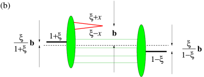
Let us first consider the GPD case (see Fig. 13a for the longitudinal momentum flow in the Efremov–Radyushkin–Brodsky–Lepage regime) in terms suitable for further generalization to TDAs. Let $x_{1}$ and $x_{2}$ be the fractions (defined with respect to average nucleon momentum $P=\frac{p_{1}+p_{2}}{2}$) of the light-cone momentum carried by an active quark and antiquark inside a nucleon. The longitudinal momentum conservation implies $x_{1}+x_{2}=2\xi$ with $\xi\geq 0$. The conventional GPD longitudinal momentum fraction variable $x$ is defined as

$$x=\frac{x_{1}-x_{2}}{2}\,.$$ (4.40)

• In the so-called Efremov–Radyushkin–Brodsky–Lepage (ERBL) region both $x_{1}$ and $x_{2}$ are positive: $x_{1},\,x_{2}\in\,[0,\,2\xi]$. In terms of the $x$ variable (4.40) it corresponds to the central region $x\in\,[-\xi,\xi]$.

• In the so-called Dokshitzer–Gribov–Lipatov–Altarelli–Parisi (DGLAP) region either $x_{1}$ is positive $x_{1}\in\,[2\xi,\,1+\xi]$ and $x_{2}$ is negative $x_{2}\in\,[-1+\xi,0]$ or vice versa ($x_{1}$ is negative $x_{1}\in\,[-1+\xi,0]$ and $x_{2}$ positive $x_{2}\in\,[2\xi,\,1+\xi]$). These two DGLAP domains result in the outer regions in terms of $x$ (4.40) $x\in[\xi,\,1]$ and $x\in[-1,\,-\xi]$ respectively.

Thus, the support properties of GPDs in terms of the momentum fraction variables $x_{1,2}$ can be summarized as

$$-1+\xi\leq x_{1,2}\leq 1+\xi;\ \ x_{1}+x_{2}=2\xi.$$ (4.41)

Figure 13: Longitudinal momentum flow in the ERBL regime for GPDs (a) and $\pi N$ TDAs (b). Small arrows show the direction of flow of positive momentum. Arrow on nucleon and quark/antiquark lines depict the flow of the baryon charge.

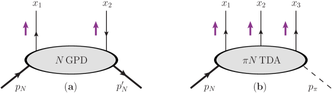
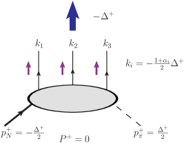
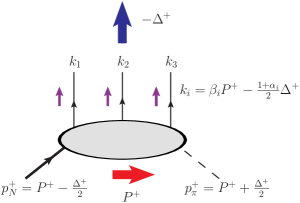
Now let us turn to the case of $\pi N$ TDAs, see Fig. 13b. The longitudinal momentum fraction variables $x_{1}$, $x_{2}$ and $x_{3}$ are defined with respect to the average hadron momentum $P=\frac{p_{1}+p_{\pi}}{2}$ (3.11) and satisfy the momentum conservation constraint $x_{1}+x_{2}+x_{3}=2\xi$, with the skewness variable (LABEL:Def_xi) $\xi\geq 0$. A natural generalization of (4.41) for the three variables satisfying the necessary symmetry and consistency conditions reads

$$-1+\xi\leq x_{i}\leq 1+\xi\ \ (i=1,\,2,\,3);\ \ x_{1}+x_{2}+x_{3}=2\xi.$$ (4.42)

Contrary to the GPD case, the shape of the complete support of TDAs depends on $\xi$. Note that in the limit $\xi\to 0$, we recover Jaffe’s results for the support property of $3$-particle parton distribution functions of higher twist established in Ref. [139].

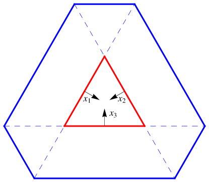
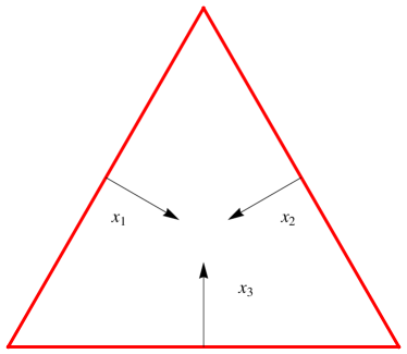
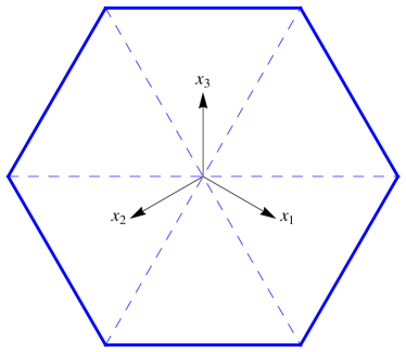
A convenient way to depict the support domain of $\pi N$ TDAs (4.42) is to employ the barycentric coordinates. The values of momentum fractions $x_{i}$ are specified by distances from a point on the plane to three sides of the equilateral triangle. The height of this equilateral triangle is defined by the momentum conservation constraint $x_{1}+x_{2}+x_{3}=2\xi$.

Figure 14: Support domain (4.42) of $\pi N$ TDAs in the longitudinal momentum fractions $x_{i}$ $i=1,\,2,\,3$ in the barycentric coordinates for $\xi=0.4$..

• First of all we identify the ERBL-like domain, in which the three longitudinal momentum fractions carried by the three quarks are positive. In the barycentric coordinates, this ERBL-like region corresponds to the interior of the equilateral triangle with the height $2\xi$ bounded by the lines $x_{i}=0$ (see Fig. 14). In Sec. 4.8 we will show that the evolution properties of TDAs within this domain are indeed governed by the ERBL-type evolution equations.

• The DGLAP-like domains are bounded by the lines

  $$x_{i}=-1+\xi\,;\ \ x_{i}=0\,;\ \ x_{i}=1+\xi\,.$$ (4.43)

  Three small equilateral triangles in Fig. 14 correspond to DGLAP-like type I domains, where only one longitudinal momentum fraction is positive while the two other ones are negative. Three trapezoid domains correspond to DGLAP-like type II, where two longitudinal momentum fractions are positive and one is negative.

Figure 15: Physical domains for $\pi N$ TDAs in the barycentric coordinates in the two limiting cases: $\xi=1$ (left) and $\xi=0$ (right). Arrows show the positive directions for momentum fractions $x_{i}$ on the barycentric plane. Note that in the case $\xi=0$ the equilateral triangle corresponding to the ERBL-like domain shrinks to a point.

In the limiting case $\xi=1$ the support domain of $\pi N$ TDAs reduces to a single ERBL-like domain, see the left panel of Fig. 15. The familiar support of nucleon DAs can be obtained by a simple rescaling of the momentum fraction variables

$$x_{i}\to\frac{x_{i}}{2}\equiv y_{i}.$$ (4.44)

In the second limiting case $\xi=0$ the ERBL-like domain shrinks to a single point and we are left with six DGLAP-like type I and II domains that form a regular hexagon in the barycentric coordinates, see the right panel of Fig. 15.

In many cases it turns out to be convenient to switch to two independent momentum fraction variables instead of $x_{i}$ that are subject to the momentum conservation constraint $\sum_{i}x_{i}=2\xi$. A natural choice of independent variables is given by the so-called quark–diquark coordinates $(w_{i};\,v_{i})$ (there exist $3$ equivalent choices $i=1,\,2,\,3$ of quark–diquark coordinates, depending on which pair of quark momenta is selected to constitute the momentum of a diquark):

$$w_{i}=x_{i}-\xi;\ \ \ v_{i}=\frac{1}{2}\sum_{k,l=1}^{3}\varepsilon_{ikl}x_{k},$$ (4.45)

where $\epsilon_{ikl}$ is the antisymmetric tensor ($\epsilon_{123}=1$).

Within these coordinates, the support of nucleon-to-meson TDAs can be parameterized as

$$-1\leq w_{i}\leq 1;\quad-1+|\xi-\xi_{i}^{\prime}|\leq v_{i}\leq 1-|\xi-\xi_{i}^{\prime}|,$$ (4.46)

where

$$\xi_{i}^{\prime}\equiv\frac{\xi-w_{i}}{2}.$$ (4.47)

The variables $\xi^{\prime}_{i}$ (4.47) characterize the longitudinal momentum fraction carried by a corresponding diquark. For example, if we choose the first and the second quarks to form a diquark

$$w_{3}=x_{3}-\xi;\ \ \ x_{1}+x_{2}=2\xi_{3}^{\prime};\ \ \ x_{1}-x_{2}=2v_{3}.$$ (4.48)

Figure 16: Support domain (4.46) of $\pi N$ TDAs in the quark–diquark coordinates $w_{3}$, $v_{3}$ for $\xi=0.4$. Dashed lines show three cross-over trajectories $w_{3}=-\xi$; $v=\pm\xi^{\prime}_{3}$ corresponding to $x_{i}=0$, $i=\{1,\,2,\,3\}$.

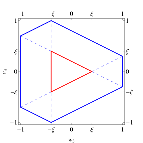
The support domain (4.46) of $\pi N$ TDAs in the quark–diquark coordinates $w_{3}$, $v_{3}$ for $\xi=0.4$ is presented in Fig. 16. Note that the ERBL-like domain (the isosceles triangle in Fig. 16) turns to be separated from the DGLAP-like domains by the cross-over trajectories

$$w_{3}=-\xi;\ \ \ v_{3}=\pm\xi_{3}^{\prime}.$$ (4.49)

The quark–diquark coordinates can be seen as a natural three-body generalization of the GPD longitudinal momentum fraction variable $x$ (4.40). In Sec. LABEL:SubSec_Bkw_meson_ampl we show that the singularities of the coefficient functions of leading order backward meson electroproduction amplitudes lie on the cross-over trajectories (4.49). This generalizes the property of the elementary LO DVCS/HMP coefficient function that is singular at $x=\pm\xi$.

In what follows, we will often present TDAs $H_{s}^{{\mathcal{M}}N}=\{V_{\Upsilon}^{{\mathcal{M}}N},\,A_{\Upsilon}^{{\mathcal{M}}N},\,T_{\Upsilon}^{{\mathcal{M}}N}\}$ as functions of a selected pair of quark–diquark coordinates instead of the longitudinal momentum fractions $x_{1,2,3}$:

$$H_{s}^{{\mathcal{M}}N}(x_{1},\,x_{2},\,x_{3}=2\xi-x_{1}-x_{2},\,\xi,\,\Delta^{2})\to H_{s}^{{\mathcal{M}}N}(w_{i},\,v_{i},\,\xi,\,\Delta^{2}).$$ (4.50)

Note that three equivalent sets of variables can be employed for the same function $H_{s}$. This reflects the underlying symmetry of our description in terms of the longitudinal momentum fractions $x_{1,2,3}$.

4.4 Polynomiality property

The Mellin moments in the longitudinal momentum fraction $x$ of GPDs are of particular importance since they are related to the form factors of local derivative operators. These objects often admit a clear physical interpretation and also can be studied within the lattice approach to QCD. The remarkable consequence of the Lorentz invariance of the underlying quantum field theory is the polynomiality property of GPDs: the $x$- Mellin moments of GPDs are polynomials of a definite power in the skewness variable.

Analogously to GPDs, nucleon-to-meson (and nucleon-to-photon) TDAs satisfy the polynomiality property. We introduce the compact notations for the $x_{i}$-Mellin moments of TDAs:

$$\langle x_{1}^{n_{1}}x_{2}^{n_{2}}x_{3}^{n_{3}}{\rm TDA}\rangle$$

$$=\int_{-1+\xi}^{1+\xi}dx_{1}\int_{-1+\xi}^{1+\xi}dx_{2}\int_{-1+\xi}^{1+\xi}dx_{3}\delta(x_{1}+x_{2}+x_{3}-2\xi)x_{1}^{n_{1}}x_{2}^{n_{2}}x_{3}^{n_{3}}{\rm TDA}(x_{1},x_{2},x_{3},\xi,\Delta^{2})\,.$$ (4.51)

Following Ref. [40], we now argue that the Mellin moments (4.51) of the leading twist nucleon-to-meson (nucleon-to-photon) TDAs are polynomials in the skewness variable $\xi$ (LABEL:Def_xi). It turns out that in the case of TDAs the situation is somewhat tricky due to the ambiguity of the choice of a set of Dirac structures in the parametrization of TDAs. The set of Dirac structures presented for $\pi N$, $VN$ and $\gamma N$ TDAs in Secs. 4.1.1–4.1.3 is convenient for the phenomenological applications since it allows a clear distinction of the subset of TDAs relevant in the $\Delta_{T}\to 0$ limit. However, as pointed out in Ref. [40], the polynomiality of the Mellin moments is spoiled by the factors $\frac{1}{1+\xi}$ that have purely kinematical origin. The manifestation of these singularities has much in common with the well known problem of construction of a set of invariant amplitudes free of kinematical singularities for a given scattering process (see e.g. Appendix II of Chapter I of [140]). In order to ensure the polynomiality property in an explicit form, one has to switch to a parametrization of TDAs with a set of Dirac structures that do not bring kinematical singularities to the Mellin moments. The general recipe consists in constructing the Dirac structures from the fully covariant component, which have no reference to a particular kinematical setup. This means that instead of the vectors $p$, $n$ and $\Delta_{T}$ one has to build the Dirac structures from the vectors $P$ and $\Delta$.

For simplicity we are going to consider the case of nucleon to pion TDAs. We omit the isospin labels for both hadronic states, as they turn out to be irrelevant for our present purpose, and consider the $3$-quark light-cone operator without reference to flavor:

$$\widehat{O}_{\rho\tau\chi}(\lambda_{1}n,\lambda_{2}n,\lambda_{3}n)=\Psi_{\rho}(\lambda_{1}n)\Psi_{\tau}(\lambda_{2}n)\Psi_{\chi}(\lambda_{3}n),$$ (4.52)

where $\Psi$ stand for the quark field operators and the color indices are omitted. We introduce an alternative parametrization for the leading twist-$3$ $\pi N$ TDAs through

$$4{\mathcal{F}}\langle\pi(p_{\pi})|\,\widehat{O}_{\rho\tau\chi}(\lambda_{1}n,\lambda_{2}n,\lambda_{3}n)\,|N(p_{N},s_{N})\rangle$$

$$=\delta({x}_{1}+{x}_{2}+{x}_{3}-2{\xi})i\frac{f_{N}}{f_{\pi}m_{N}}\sum_{s}(s^{\pi N})_{\rho\tau,\,\chi}H_{s}^{\pi N}(x_{1},x_{2},x_{3},\xi,\Delta^{2};\,\mu^{2}),$$ (4.53)

where we employ the shortened notations for the set of invariant $\pi N$ TDAs

$$H_{s}^{\pi N}=\bigl{\{}V_{1,2}^{\pi N},\,A_{1,2}^{\pi N},\,T_{1,2,3,4}^{\pi N}\bigr{\}}\,.$$ (4.54)

The sum in (4.53) stands over the set of the leading twist-$3$ Dirac structures

$$(s^{\pi N})_{\rho\tau,\,\chi}=\bigl{\{}(v_{1,2}^{\pi N})_{\rho\tau,\,\chi},\,(a_{1,2}^{\pi N})_{\rho\tau,\,\chi},(t_{1,2,3,4}^{\pi N})_{\rho\tau,\,\chi}\bigr{\}}.$$ (4.55)

The explicit expressions for the set of Dirac structures in (4.53) read:

$$(v_{1}^{\pi N})_{\rho\tau,\,\chi} =(\hat{P}C)_{\rho\tau}(\hat{P}U)_{\chi}\,; (v_{2}^{\pi N})_{\rho\tau,\,\chi} =(\hat{P}C)_{\rho\tau}(\hat{\Delta}U)_{\chi}\,;{}$$

$$(a_{1}^{\pi N})_{\rho\tau,\,\chi} =(\hat{P}\gamma^{5}C)_{\rho\tau}(\gamma^{5}\hat{P}U)_{\chi}\,; (a_{2}^{\pi N})_{\rho\tau,\,\chi} =(\hat{P}\gamma^{5}C)_{\rho\tau}(\gamma^{5}\hat{\Delta}U)_{\chi}\,;{}$$

$$(t_{1}^{\pi N})_{\rho\tau,\,\chi} =(\sigma_{P\mu}C)_{\rho\tau}(\gamma^{\mu}\hat{P}U)_{\chi}\,;M (t_{2}^{\pi N})_{\rho\tau,\,\chi} =(\sigma_{P\mu}C)_{\rho\tau}(\gamma^{\mu}\hat{\Delta}U)_{\chi}\,;$$

$$(t_{3}^{\pi N})_{\rho\tau,\,\chi} =m_{N}^{-1}(\sigma_{P\Delta}C)_{\rho\tau}(\hat{P}U)_{\chi}\,; (t_{4}^{\pi N})_{\rho\tau,\,\chi} =m_{N}^{-1}(\sigma_{P\Delta}C)_{\rho\tau}(\hat{\Delta}U)_{\chi}\,.$$ (4.56)

As a consequence of the Dirac equation (4.8) we establish the following identities:

$$(\hat{P}\,U(p_{N},s_{N}))_{\chi}$$

$$=\frac{m_{N}}{1+\xi}U^{+}(p_{N},s_{N})_{\chi}+\frac{1}{2}(\hat{\Delta}_{T}U(p_{N},s_{N}))_{\chi}+\frac{(1+\xi)}{2m_{N}}\left[\frac{m^{2}_{N}}{1+\xi}+\frac{m_{\pi}^{2}-\Delta_{T}^{2}}{1-\xi}\right]U^{-}(p_{N},s_{N})_{\chi}\,;$$ (4.57)

$$(\hat{\Delta}\,U(p_{N},s_{N}))_{\chi}$$

$$=-2\xi\frac{m_{N}}{1+\xi}U^{+}(p_{N},s_{N})_{\chi}+(\hat{\Delta}_{T}U(p_{N},s_{N}))_{\chi}-\frac{(1+\xi)}{m_{N}}\left[\frac{m_{N}^{2}}{1+\xi}-\frac{m^{2}_{\pi}-\Delta_{T}^{2}}{1-\xi}\right]U^{-}(p_{N},s_{N})_{\chi}\,.$$ (4.58)

The last terms in Eqs. (4.57), (4.58) are of sub-leading twist while the two first terms are of the leading twist. Then, to the leading twist-$3$ accuracy, the relation of new $\pi N$ TDA definition (4.53) with the set of Dirac structures (4.56) of $\pi N$ TDAs to that of Eq. (4.4) with the set of Dirac structures (4.6) is given by

$$\left.{\{V_{1},A_{1},T_{1}\}^{\pi N}}\right|_{\text{set of Eq.\leavevmode\nobreak\ (\ref{Def_DirStr_piN_DeltaT})}}=\left.\left(\frac{1}{1+\xi}\{V_{1},A_{1},T_{1}\}^{\pi N}-\frac{2\xi}{1+\xi}\{V_{2},A_{2},T_{2}\}^{\pi N}\right)\right|_{\text{set of Eq.\leavevmode\nobreak\ (\ref{Dirac_structures_PiN_TDA_Cov})}}\,;$$

$$\left.{\{V_{2},A_{2}\}^{\pi N}}\right|_{\text{set of Eq.\leavevmode\nobreak\ (\ref{Def_DirStr_piN_DeltaT})}}=\left.\left({\{V_{2},A_{2}\}^{\pi N}}+\frac{1}{2}{\{V_{1},A_{1}\}^{\pi N}}\right)\right|_{\text{set of Eq.\leavevmode\nobreak\ (\ref{Dirac_structures_PiN_TDA_Cov})}}\,;$$

$$\left.{T_{3}^{\pi N}}\right|_{\text{set of Eq.\leavevmode\nobreak\ (\ref{Def_DirStr_piN_DeltaT})}}=\left.\left({T_{2}^{\pi N}}+\frac{1}{2}{T_{1}^{\pi N}}\right)\right|_{\text{set of Eq.\leavevmode\nobreak\ (\ref{Dirac_structures_PiN_TDA_Cov})}};$$

$$\left.{T_{2}^{\pi N}}\right|_{\text{set of Eq.\leavevmode\nobreak\ (\ref{Def_DirStr_piN_DeltaT})}}=\left.\left(\frac{1}{2}T_{1}^{\pi N}+T_{2}^{\pi N}+T_{3}^{\pi N}-2\xi T_{4}^{\pi N}\right)\right|_{\text{set of Eq.\leavevmode\nobreak\ (\ref{Dirac_structures_PiN_TDA_Cov})}}\,;$$

$$\left.{T_{4}^{\pi N}}\right|_{\text{set of Eq.\leavevmode\nobreak\ (\ref{Def_DirStr_piN_DeltaT})}}=\left.\left(\frac{1+\xi}{2}T_{3}^{\pi N}+(1+\xi){T_{4}^{\pi N}}\right)\right|_{\text{set of Eq.\leavevmode\nobreak\ (\ref{Dirac_structures_PiN_TDA_Cov})}}\,.$$ (4.59)

Now we proceed with the Mellin moments of $\pi N$ TDAs defined in Eq. (4.53) with the fully covariant set of leading twist Dirac structures (4.56). The $(n_{1},n_{2},n_{3})$-th Mellin moments ($n_{1}+n_{2}+n_{3}=N$) of the TDAs in $x_{1}$, $x_{2}$, $x_{3}$ lead to derivative operations acting on the three quark fields:

$$4(P\cdot n)^{n_{1}+n_{2}+n_{3}+3}\int d^{3}x\,x_{1}^{n_{1}}x_{2}^{n_{2}}x_{3}^{n_{3}}$$

$$\int\left[\prod_{k=1}^{3}\frac{d\lambda_{k}}{2\pi}\right]e^{i\sum_{k=1}^{3}x_{k}\lambda_{k}(P\cdot n)}\langle\pi(P+\frac{\Delta}{2})|\widehat{O}_{\rho\,\tau\,\chi}(\lambda_{1}n,\,\lambda_{2}n,\,\lambda_{3}n)|N(P-\frac{\Delta}{2})\rangle$$

$$=(P\cdot n)^{n_{1}+n_{2}+n_{3}}\frac{if_{N}}{f_{\pi}m_{N}}\sum_{s}(s^{\pi N})_{\rho\tau,\,\chi}\int_{-1+\xi}^{1+\xi}dx_{1}\int_{-1+\xi}^{1+\xi}dx_{2}\int_{-1+\xi}^{1+\xi}dx_{3}\,x_{1}^{n_{1}}x_{2}^{n_{2}}x_{3}^{n_{3}}$$

$$\times\delta(x_{1}+x_{2}+x_{3}-2\xi)H_{s}^{\pi N}(x_{1},x_{2},x_{3},\xi,\Delta^{2})$$

$$=4(-1)^{n_{1}+n_{2}+n_{3}}\langle\pi(P+\frac{\Delta}{2})|\left[(i\vec{\partial}^{+})^{n_{1}}\Psi_{\rho}(0)\right]\left[(i\vec{\partial}^{+})^{n_{2}}\Psi_{\tau}(0)\right]\left[(i\vec{\partial}^{+})^{n_{3}}\Psi_{\chi}(0)\right]|N(P-\frac{\Delta}{2})\rangle\,.$$ (4.60)

Hence, the Mellin moments of nucleon to meson TDAs are expressed through the form factors of the local twist-$3$ operators:

$$\widehat{O}_{\rho\tau\chi}^{\;\mu_{1}...\mu_{n_{1}},\,\nu_{1}...\nu_{n_{2}},\,\lambda_{1}...\lambda_{n_{3}}}(0)=\left[i\vec{D}^{\mu_{1}}...\,i\vec{D}^{\mu_{n_{1}}}\Psi_{\rho}\right]\left[i\vec{D}^{\nu_{1}}...\,i\vec{D}^{\nu_{n_{2}}}\Psi_{\tau}\right]\left[i\vec{D}^{\lambda_{1}}...\,i\vec{D}^{\lambda_{n_{3}}}\Psi_{\chi}\right]\,,$$ (4.61)

where

$$\vec{D}^{\mu}=\vec{\partial}^{\mu}-igA^{a\,\mu}t^{a}$$ (4.62)

is the covariant derivative. Here $t^{a}=\frac{\lambda^{a}}{2}$ with $\lambda^{a}$, $a=1,\ldots,8$ being the Gell-Mann matrices. Note that in (4.60), (4.61) the color indices are omitted.

Introducing the shortened notation

$$(\Delta^{\mu})^{i}(P^{\mu})^{n_{1}-i}\equiv\Delta^{\mu_{1}}...\Delta^{\mu_{i}}P^{\mu_{i+1}}...P^{\mu_{n_{1}}}$$ (4.63)

we write down the following parametrization for the $\pi N$ matrix element of the local operator (4.61):

$$4\langle\pi|\widehat{O}_{\rho\tau\chi}^{\;\mu_{1}...\mu_{n_{1}},\,\nu_{1}...\nu_{n_{2}},\,\lambda_{1}...\lambda_{n_{3}}}(0)|N\rangle=i\frac{f_{N}}{f_{\pi}m_{N}}$$

$$\times\Bigl{[}\sum_{s}(s^{\pi N})_{\rho\tau,\,\chi}\sum_{i=0}^{n_{1}}\sum_{j=0}^{n_{2}}\sum_{k=0}^{n_{3}}A^{s\;(n_{1},n_{2},n_{3})}_{ijk}(\Delta^{2})(\Delta^{\mu})^{i}(P^{\mu})^{n_{1}-i}(\Delta^{\nu})^{j}(P^{\nu})^{n_{2}-j}(\Delta^{\lambda})^{i}(P^{\lambda})^{n_{3}-i}$$

$$+\left\{(\hat{\Delta}C)_{\rho\tau}(\hat{P}U)_{\chi}C^{V_{1}\;(n_{1},n_{2},n_{3})}_{N+1}(\Delta^{2})+(\hat{\Delta}C)_{\rho\tau}(\hat{\Delta}U)_{\chi}C^{V_{2}\;(n_{1},n_{2},n_{3})}_{N+1}(\Delta^{2})\right.$$

$$\left.+(\hat{\Delta}\gamma^{5}C)_{\rho\tau}(\gamma^{5}\hat{P}U)_{\chi}C^{A_{1}\;(n_{1},n_{2},n_{3})}_{N+1}(\Delta^{2})+(\hat{\Delta}\gamma^{5}C)_{\rho\tau}(\gamma^{5}\hat{\Delta}U)_{\chi}C^{A_{2}\;(n_{1},n_{2},n_{3})}_{N+1}(\Delta^{2})\right.$$

$$\left.+(\sigma_{\Delta\mu}C)_{\rho\tau}(\gamma^{\mu}\hat{P}U)_{\chi}C^{T_{1}\;(n_{1},n_{2},n_{3})}_{N+1}(\Delta^{2})+(\sigma_{\Delta\mu}C)_{\rho\tau}(\gamma^{\mu}\hat{\Delta}U)_{\chi}C^{T_{2}\;(n_{1},n_{2},n_{3})}_{N+1}(\Delta^{2})\right\}$$

$$\times(\Delta^{\mu})^{n_{1}}(\Delta^{\nu})^{n_{2}}(\Delta^{\lambda})^{n_{3}}\Bigr{]}\,,$$ (4.64)

where the sum in the first term is over the set of Dirac structures (4.56); and $A^{s\;(n_{1},n_{2},n_{3})}_{ijk}(\Delta^{2})$ and $C^{V_{1,2},\,A_{1,2},\,T_{1,2}\;(n_{1},n_{2},n_{3})}_{N+1}(\Delta^{2})$ denote the appropriate invariant form factors.

Now from (4.64) we establish the following relations for $(n_{1},\,n_{2},\,n_{3})$-th Mellin moments of the TDAs:

$$\langle x_{1}^{n_{1}}x_{2}^{n_{2}}x_{3}^{n_{3}}\{V_{1,2}^{\pi N},\,A_{1,2}^{\pi N},\,T_{1,2}^{\pi N}\}\rangle$$

$$=\sum_{n=0}^{N}(-1)^{N-n}(2\xi)^{n}\sum_{i=0}^{n_{1}}\sum_{j=0}^{n_{2}}\sum_{k=0}^{n_{3}}\delta_{i+j+k,\,n}\;A^{\{V_{1,2},\,A_{1,2},\,T_{1,2}\}\;(n_{1},n_{2},n_{3})}_{ijk}(\Delta^{2})+(-2\xi)^{N+1}C^{\{V_{1,2},\,A_{1,2},\,T_{1,2}\}\;(n_{1},n_{2},n_{3})}_{N+1}(\Delta^{2})\,;$$

$$\langle x_{1}^{n_{1}}x_{2}^{n_{2}}x_{3}^{n_{3}}\{T_{3,4}^{\pi N}\}\rangle=\sum_{n=0}^{N}(-1)^{N-n}(2\xi)^{n}\sum_{i=0}^{n_{1}}\sum_{j=0}^{n_{2}}\sum_{k=0}^{n_{3}}\delta_{i+j+k,\,n}\;A^{\{T_{3,4}\}\;(n_{1},n_{2},n_{3})}_{ijk}(\Delta^{2})\,,$$ (4.65)

which demonstrates that the $\pi N$ TDAs defined in (4.53) indeed satisfy the polynomiality property. Let us emphasize that, contrary to the GPD case, the discrete symmetries do not impose any restrictions for evenness/oddness of the Mellin moments of TDAs and $n_{1,2,3}$ are arbitrary integers.

• For $n_{1}+n_{2}+n_{3}=N$ the highest power of $\xi$ occurring in $(n_{1},n_{2},n_{3})$-th Mellin moment of $\{V_{1,2}^{\pi N},\,A_{1,2}^{\pi N},\,T_{1,2}^{\pi N}\}$ is $N+1$.

• For $T_{3,4}^{\pi N}$ the highest power of $\xi$ occurring in $(n_{1},n_{2},n_{3})$-th Mellin moment is $N$.

Consequently, the TDAs $\{V_{1,2}^{\pi N},\,A_{1,2}^{\pi N},\,T_{1,2}^{\pi N}\}$ include an analogue of the $D$-term contribution [74] that generates the highest possible power of $\xi$ for a given Mellin moment.

4.5 A spectral representation

The double distribution representation of GPDs [66, 141, 142, 73] incorporates both the polynomiality property of the Mellin moments and the support properties of GPDs. In [75] it was pointed out that the relation between a GPD and the corresponding DD is a particular case of the Radon transform. The polynomiality property is well known in the framework of the Radon transform theory as the Cavalieri conditions [143].

In this subsection, following Ref. [39], we present a generalization of a spectral representation for TDAs, that ensures the support properties of Sec. 4.3 and the polynomiality property of the corresponding Mellin moments (4.65). Throughout this subsection we consider $\pi N$ TDAs introduced within the fully covariant parametrization (4.53) with the set of the Dirac structures (4.56), that ensures the polynomiality property in its simple form.

4.5.1 A symmetric form of the spectral representation for GPDs

In the framework of the DD representation a GPD $H$ is given as a one dimensional section of the double distribution (DD) $f(\alpha,\beta)$:

$$H(x,\,\xi)=\int_{\Omega}d\beta d\alpha\,\delta(x-\beta-\alpha\xi)f(\beta,\,\alpha)\,.$$ (4.66)

The spectral representation (4.66) was originally recovered from the diagrammatic analysis employing the $\alpha$-representation techniques [90, 89]. The restricted integration domain

$$\Omega=\{|\beta|\leq 1;\ \ \ |\alpha|\leq 1-|\beta|\};$$ (4.67)

ensures the support property of GPDs $|x|\leq 1$ for any $|\xi|\leq 1$. The polynomiality property of the $x$-Mellin moments of GPDs turns out to be an intrinsic feature of the DD representation (4.66).

In order to generalize the spectral representation (4.66) for the three-parton case we need to rewrite it in a symmetric form as a function of the momentum fraction variables $x_{1,2}$ (4.41). The partonic momentum fractions $x_{1,2}$ are supposed to have the following decomposition in terms of the spectral parameters:

$$x_{1}=\beta_{1}+(1+\alpha_{1})\xi\,;\ \ \ x_{2}=\beta_{2}+(1+\alpha_{2})\xi\,.$$ (4.68)

This allows us to write down the following spectral representation for GPD $H(x_{1},\,x_{2}=2\xi-x_{1},\,\xi)$:

$$H(x_{1},\,x_{2}=2\xi-x_{1},\,\xi)$$

$$=\int_{\Omega_{1}}d\beta_{1}d\alpha_{1}\int_{\Omega_{2}}d\beta_{2}d\alpha_{2}\delta(x_{1}-\xi-\beta_{1}-\alpha_{1}\xi)\delta(\beta_{1}+\beta_{2})\delta(\alpha_{1}+\alpha_{2})F(\beta_{1},\beta_{2},\alpha_{1},\alpha_{2})\,.$$ (4.69)

Here $\Omega_{1,2}$ are the usual domains (4.67) in the spectral parameter space. The momentum conservation condition $x_{1}+x_{2}=2\xi$ is imposed by two $\delta$-functions $\delta(\beta_{1}+\beta_{2})\delta(\alpha_{1}+\alpha_{2})$. The spectral density $F(\beta_{1},\beta_{2},\alpha_{1},\alpha_{2})$ is thus a function of four variables that is subject to two constraints, imposed by two $\delta$-functions, hence effectively it is a double distribution.

To show that the spectral representation (4.69) is equivalent to the usual DD representation (4.66) the two superfluous integrations must be lifted with the help of two $\delta$-functions. As pointed out in Ref. [39], this problem can be solved by switching to the set of natural spectral variables

$$\alpha_{\pm}=\frac{\alpha_{1}\pm\alpha_{2}}{2}\,;\ \ \ \beta_{\pm}=\frac{\beta_{1}\pm\beta_{2}}{2}\,.$$ (4.70)

and the appropriate combinations of the longitudinal momentum fraction variables

$$x_{\pm}=\frac{x_{1}\pm x_{2}}{2}\,.$$ (4.71)

Performing the integration in $\beta_{+}$ and $\alpha_{+}$ is straightforward (see Sec. IV.A of Ref. [39]). It does not bring additional restrictions on the remaining spectral parameters $\alpha_{-}$, $\beta_{-}$. The result reads

$$H(x_{1},\,x_{2}=2\xi-x_{1},\,\xi)=\int_{-1}^{1}d\beta_{-}\int_{-1+|\beta_{-}|}^{1-|\beta_{-}|}d\alpha_{-}\delta(x_{-}-\beta_{-}-\alpha_{-}\xi)2F\left(\beta_{-},-\beta_{-},\alpha_{-},-\alpha_{-}\right)\,.$$ (4.72)

Since $x_{-}\equiv x$, by renaming the integration variables $\alpha_{-}\to\alpha$, $\beta_{-}\to\beta$ and introducing the DD

$$f(\beta,\,\alpha)\equiv 2F\left(\beta,-\beta,\alpha,-\alpha\right)$$ (4.73)

one recovers the usual form of the DD representation (4.66).

For completeness we also present the expressions for a GPD in various domains in $x$, that results from performing the $\alpha$-integration in Eq. (4.66) with the help of the $\delta$-function. For arbitrary $0\leq\xi\leq 1$ we get the following:

• $|x|>1$:

  $$H(x,\xi)=0;$$ (4.74)

• DGLAP domain $-1\leq x\leq-\xi$:

  $$H\left(x,\xi\right)=\frac{1}{\xi}\int_{\frac{x-\xi}{1+\xi}}^{\frac{x+\xi}{1-\xi}}\mathrm{d}\beta F\left(\beta,\frac{x-\beta}{\xi}\right);$$ (4.75)

• ERBL domain $-\xi\leq x\leq\xi$:

  $$H\left(x,\xi\right)=\frac{1}{\xi}\int_{\frac{x-\xi}{1+\xi}}^{\frac{x+\xi}{1+\xi}}\mathrm{d}\beta F\left(\beta,\frac{x-\beta}{\xi}\right);$$ (4.76)

• DGLAP domain $\xi\leq x\leq 1$:

  $$H\left(x,\xi\right)=\frac{1}{\xi}\int_{\frac{x-\xi}{1-\xi}}^{\frac{x+\xi}{1+\xi}}\mathrm{d}\beta F\left(\beta,\frac{x-\beta}{\xi}\right).$$ (4.77)

4.5.2 Quadruple distributions

The spectral representation for a $\pi N$ TDA $H(x_{1},\,x_{2},\,x_{3}=2\xi-x_{1}-x_{2},\,\xi)$ can be written as a straightforward generalization of the spectral representation for GPDs (4.69).

Following Section 3.8 of Ref. [13], we take a point of view on TDAs, as kinematic “hybrids” of forward 3-parton densities and of distribution amplitudes and represent the corresponding momentum flow as a superposition of the $s$-channel and $t$-channel momentum fluxes (see Fig. 17).

Figure 17: Momentum flow in a quadruple distribution (right panel) as a superposition of the momentum flow of a forward density (left panel) and of a distribution amplitude (central panel).

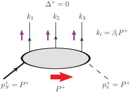
We introduce three sets of spectral parameters $\beta_{1,2,3}$, $\alpha_{1,2,3}$. The longitudinal momentum fractions of the three quarks $x_{1,2,3}$ are supposed to have the following decomposition in terms of the spectral parameters:

$$x_{1}=\xi+\beta_{1}+\alpha_{1}\xi\,;\ \ \ x_{2}=\xi+\beta_{2}+\alpha_{2}\xi\,;\ \ \ x_{3}=\xi+\beta_{3}+\alpha_{3}\xi\,.$$ (4.78)

In order to satisfy the momentum conservation constraint $\sum_{i}x_{i}=2\xi$ we require that

$$\beta_{1}+\beta_{2}+\beta_{3}=0\,;\ \ \ \alpha_{1}+\alpha_{2}+\alpha_{3}=-1\,.$$ (4.79)

This allows us to write down the following spectral representation for $\pi N$ TDAs:

$$H(x_{1},\,x_{2},\,x_{3}=2\xi-x_{1}-x_{2},\,\xi)$$

$$=\left[\prod_{i=1}^{3}\int_{\Omega_{i}}d\beta_{i}d\alpha_{i}\right]\delta(x_{1}-\xi-\beta_{1}-\alpha_{1}\xi)\,\delta(x_{2}-\xi-\beta_{2}-\alpha_{2}\xi)\,$$

$$\times\delta(\beta_{1}+\beta_{2}+\beta_{3})\delta(\alpha_{1}+\alpha_{2}+\alpha_{3}+1)F(\beta_{1},\,\beta_{2},\,\beta_{3},\,\alpha_{1},\,\alpha_{2},\alpha_{3})\,.$$ (4.80)

By $\Omega_{i},\,i=\left\{1,\,2,\,3\right\}$ we denote the three copies of the usual domains (4.67) in the spectral parameter space. The spectral density $F(\beta_{1},\,\beta_{2},\,\beta_{3},\,\alpha_{1},\,\alpha_{2},\alpha_{3})$ is a function of $6$ variables (sextuple distribution). However, these variables are subject to two constraints. Therefore, effectively $F$ turns out to be a quadruple distribution.

To clarify the physical contents of the quadruple distribution it is instructive to consider the following spectral representation in terms of quadruple distributions which can be established for $\pi N$ matrix element of the twist-$3$ non-local $3$-quark light-cone operator (4.52):

$$\langle\pi(p_{\pi})|\widehat{O}_{\rho\tau\chi}(\lambda_{1}n,\,\,\lambda_{2}n,\,\lambda_{3}n)|p(p_{N})\rangle{}$$

$$=\frac{1}{4(P\cdot n)}i\frac{f_{N}}{f_{\pi}m_{N}}\left[\prod_{i=1}^{3}\int_{-1+\xi}^{1+\xi}dx_{i}\right]\delta(2\xi-x_{1}-x_{2}-x_{3})e^{-i\sum_{k}x_{k}\lambda_{k}(P\cdot n)}\sum_{s}(s^{\pi N})_{\rho\tau,\,\chi}H_{s}(x_{1},x_{2},x_{3},\xi){}$$

$$=i\frac{f_{N}}{f_{\pi}m_{N}}\left[\prod_{i=1}^{3}\int_{\Omega_{i}}d\beta_{i}d\alpha_{i}\right]e^{-\sum_{k}\beta_{k}\lambda_{k}(P\cdot n)-i\sum_{l}\alpha_{l}\lambda_{l}(-\Delta\cdot n)}\delta(\beta_{1}+\beta_{2}+\beta_{3})\delta(\alpha_{1}+\alpha_{2}+\alpha_{3}+1){}$$

$$\sum_{s}(s^{\pi N})_{\rho\tau,\,\chi}F_{s}(\beta_{1},\,\beta_{2},\,\beta_{3},\,\alpha_{1},\,\alpha_{2},\alpha_{3}),$$ (4.81)

where the momentum flow in the quadruple distributions is specified in Fig. 17. We denote here by $F_{s}(\beta_{1},\,\beta_{2},\,\beta_{3},\,\alpha_{1},\,\alpha_{2},\alpha_{3})$ the spectral density corresponding to a particular TDA $H_{s}$ occurring in the Dirac decomposition of the matrix element in the l.h.s. of Eq. (4.81). The formula (4.81) can be seen as a straightforward generalization of the familiar spectral representation for the matrix element of the composite operator $\phi\phi$ constructed out of scalar fields (see e.g. discussion around Eq. (3.206) in Section 3.8 of Ref. [13]).

Now we need to verify that $\pi N$ TDAs within the spectral representation (4.80) satisfy the polynomiality property and possess the correct support properties (4.42) in the longitudinal momentum fraction $x_{i}$.

Checking the polynomiality property is an easy task. By a formal interchange of integration order we show that the $(n_{1},\,n_{2},\,n_{3})$-th Mellin moment in $(x_{1},\,x_{2},\,x_{3})$ of $\pi N$ TDA is, indeed, a polynomial of order $N\equiv n_{1}+n_{2}+n_{3}$ of $\xi$:

$$\langle x_{1}^{n_{1}}x_{2}^{n_{2}}x_{3}^{n_{3}}H(x_{1},\,x_{2},\,x_{3}=2\xi-x_{1}-x_{2},\,\xi)\rangle{}$$

$$=\left[\prod_{i=1}^{3}\int_{\Omega_{i}}d\beta_{i}d\alpha_{i}\right]\left[\prod_{j=1}^{3}\int_{-1+\xi}^{1+\xi}dx_{j}\right]\delta(\beta_{1}+\beta_{2}+\beta_{3})\delta(\alpha_{1}+\alpha_{2}+\alpha_{3}+1)F(\beta_{1},\,\beta_{2},\,\beta_{3},\,\alpha_{1},\,\alpha_{2},\alpha_{3}){}$$

$$\times x_{1}^{n_{1}}x_{2}^{n_{2}}x_{3}^{n_{3}}\,\delta(x_{1}+x_{2}+x_{3}-2\xi)\,\delta(x_{1}-\xi-\beta_{1}-\alpha_{1}\xi)\,\delta(x_{2}-\xi-\beta_{2}-\alpha_{2}\xi)=P_{N}(\xi)\,.$$ (4.82)

Working out the support properties of (4.80) follows the same stages as the derivation of Sec. 4.5.1. The first step consists in switching to natural combinations of spectral parameters and performing two out of the six integrals in (4.80). At the second step we work out the support properties and derive the analogue of Eqs. (4.75)–(4.77) for TDAs in the various domains of the support.

There exist there equivalent choices of convenient combinations of spectral parameters $\sigma_{i}$, $\rho_{i}$, $\omega_{i}$, $\nu_{i}$ that are adjusted with the three sets of quark–diquark coordinates $(w_{i},\,v_{i})$ (4.45):

$$\sigma_{i}=\beta_{i};\ \ \ \rho_{i}=\sum_{k,l=1}^{3}\varepsilon_{ikl}\beta_{k};{}$$

$$\omega_{i}=\alpha_{i}\,;\ \ \ \nu_{i}=\sum_{k,l=1}^{3}\varepsilon_{ikl}\alpha_{k}.$$ (4.83)

Performing two integrals over spectral parameters (see Sec. IV and Appendix A of Ref. [39]) results in three equivalent representation of $\pi N$ TDAs as a function of quark–diquark coordinates $w_{i},\,v_{i}$:

$$H(w_{i},\,v_{i},\,\xi)$$

$$=\int_{-1}^{1}d\sigma_{i}\int_{-1+\frac{|\sigma_{i}|}{2}}^{1-\frac{|\sigma_{i}|}{2}}d\rho_{i}\int_{-1+|\sigma_{i}|}^{1-|\rho_{i}-\frac{\sigma_{i}}{2}|-|\rho_{i}+\frac{\sigma_{i}}{2}|}d\omega_{i}\int_{-\frac{1}{2}+|\rho_{i}-\frac{\sigma_{i}}{2}|+\frac{\omega_{i}}{2}}^{\frac{1}{2}-|\rho_{i}+\frac{\sigma_{i}}{2}|-\frac{\omega_{i}}{2}}d\nu_{i}\delta(w_{i}-\sigma_{i}-\omega_{i}\xi)$$

$$\times\delta(v_{i}-\rho_{i}-\nu_{i}\xi)\,F_{i}(\sigma_{i},\,\rho_{i},\,\omega_{i},\,\nu_{i})\,.$$ (4.84)

The quadruple distributions $F_{i}$ are expressed in three equivalent forms in terms of the master sextuple distribution defined in Eq. (4.80) (cf. Eq. (4.73) for the GPD case):

$$F_{1}(\sigma_{1},\,\rho_{1},\,\omega_{1},\,\nu_{1})\equiv F(\sigma_{1},\,\rho_{1}-\frac{\sigma_{1}}{2}\,,-\rho_{1}-\frac{\sigma_{1}}{2},\,\omega_{1},\,\nu_{1}-\frac{1+\omega_{1}}{2},\,-\nu_{1}-\frac{1+\omega_{1}}{2})\,;$$

$$F_{2}(\sigma_{2},\,\rho_{2},\,\omega_{2},\,\nu_{2})\equiv F(-\rho_{2}-\frac{\sigma_{2}}{2},\,\sigma_{2},\,\rho_{2}-\frac{\sigma_{2}}{2},\,-\nu_{2}-\frac{1+\omega_{2}}{2},\,\omega_{2},\,\nu_{2}-\frac{1+\omega_{2}}{2})\,;$$

$$F_{3}(\sigma_{3},\,\rho_{3},\,\omega_{3},\,\nu_{3})\equiv F(\rho_{3}-\frac{\sigma_{3}}{2},\,-\rho_{3}-\frac{\sigma_{3}}{2},\,\sigma_{3},\,\nu_{3}-\frac{1+\omega_{3}}{2},\,-\nu_{3}-\frac{1+\omega_{3}}{2},\omega_{3})\,.$$ (4.85)

The next step consists in establishing a generalization of Eqs. (4.74)–(4.77) expressing $\pi N$ TDAs in different parts of the support domain (4.46). It is done by performing two integrals over the spectral parameters $\omega_{i}$, $\nu_{i}$ in (4.84) with the help of the two $\delta$-functions. This analysis is rather technical and requires careful treatment of the integration limits in corresponding multiple integrals. For the details of derivation we refer the reader to Sec. V of Ref. [39].

Figure 18: Spectral representation for $\pi N$ TDA (4.84) in the ERBL-like and DGLAP-like type I, II domains in the quark–diquark coordinates $w_{i}$, $v_{i}$ (4.45) for $\xi=0.4$.

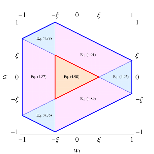
For $0\leq\xi\leq 1$, depending on the part of the ($w_{i}\,;\,v_{i}$) support domain in question, the quadruple integral (4.84) for $H(w,v,\xi)$ reduces to the following expressions (see Fig. 18):

• DGLAP-like type I domain $w_{i}\in[-1;\,-\xi]$; $v_{i}\in[\xi^{\prime}_{i};\,1-\xi^{\prime}_{i}+\xi]$ ($\xi^{\prime}_{i}\equiv\frac{\xi-w_{i}}{2}$):

  $$H(w_{i},\,v_{i},\xi)=\frac{1}{\xi^{2}}\int_{\frac{2(v_{i}\xi-\xi^{\prime}_{i})}{1-\xi^{2}}}^{\frac{w_{i}+\xi}{1-\xi}}d\sigma_{i}\int_{-\frac{\sigma_{i}}{2}+\frac{v_{i}-\xi^{\prime}_{i}}{1-\xi}}^{\frac{\sigma_{i}}{2}+\frac{v_{i}+\xi^{\prime}_{i}}{1+\xi}}d\rho_{i}\,F_{i}(\sigma_{i},\,\rho_{i},\,\frac{w_{i}-\sigma_{i}}{\xi},\,\frac{v_{i}-\rho_{i}}{\xi})\,;$$ (4.86)

• DGLAP-like type II domain $w_{i}\in[-1;\,-\xi]$; $v_{i}\in[-\xi^{\prime}_{i};\,\xi^{\prime}_{i}]$:

  $$H(w_{i},\,v_{i},\xi)=\frac{1}{\xi^{2}}\int_{\frac{w_{i}-\xi}{1+\xi}}^{\frac{w_{i}+\xi}{1-\xi}}d\sigma_{i}\int_{-\frac{\sigma_{i}}{2}+\frac{v_{i}-\xi^{\prime}_{i}}{1+\xi}}^{\frac{\sigma_{i}}{2}+\frac{v_{i}+\xi^{\prime}_{i}}{1+\xi}}d\rho_{i}\,F_{i}(\sigma_{i},\,\rho_{i},\,\frac{w_{i}-\sigma_{i}}{\xi},\,\frac{v_{i}-\rho_{i}}{\xi})\,;$$ (4.87)

• DGLAP-like type I domain $w_{i}\in[-1;\,-\xi]$; $v_{i}\in[-1+\xi^{\prime}_{i}-\xi;\,-\xi^{\prime}_{i}]$ :

  $$H(w_{i},\,v_{i},\xi)=\frac{1}{\xi^{2}}\int_{-\frac{2(v_{i}\xi+\xi^{\prime}_{i})}{1-\xi^{2}}}^{\frac{w_{i}+\xi}{1-\xi}}d\sigma_{i}\int_{-\frac{\sigma_{i}}{2}+\frac{v_{i}-\xi^{\prime}_{i}}{1+\xi}}^{\frac{\sigma_{i}}{2}+\frac{v_{i}+\xi^{\prime}_{i}}{1-\xi}}d\rho_{i}\,F_{i}(\sigma_{i},\,\rho_{i},\,\frac{w_{i}-\sigma_{i}}{\xi},\,\frac{v_{i}-\rho_{i}}{\xi})\,;$$ (4.88)

• DGLAP-like type II domain $w_{i}\in[-\xi;\,1]$; $v_{i}\in[-1+\xi-\xi^{\prime}_{i};\,-|\xi^{\prime}_{i}|]$:

  $$H(w_{i},\,v_{i},\xi)=\frac{1}{\xi^{2}}\int_{-\frac{2(v_{i}\xi+\xi^{\prime}_{i})}{1-\xi^{2}}}^{\frac{w_{i}+\xi}{1+\xi}}d\sigma_{i}\int_{-\frac{\sigma_{i}}{2}+\frac{v_{i}-\xi^{\prime}_{i}}{1+\xi}}^{\frac{\sigma_{i}}{2}+\frac{v_{i}+\xi^{\prime}_{i}}{1-\xi}}d\rho_{i}\,F_{i}(\sigma_{i},\,\rho_{i},\,\frac{w_{i}-\sigma_{i}}{\xi},\,\frac{v_{i}-\rho_{i}}{\xi})\,;$$ (4.89)

• ERBL-like domain $w_{i}\in[-\xi;\,\xi]$; $v_{i}\in[-\xi^{\prime}_{i};\,\xi^{\prime}_{i}]$:

  $$H(w_{i},\,v_{i},\xi)=\frac{1}{\xi^{2}}\int_{\frac{w_{i}-\xi}{1+\xi}}^{\frac{w_{i}+\xi}{1+\xi}}d\sigma_{i}\int_{-\frac{\sigma_{i}}{2}+\frac{v_{i}-\xi^{\prime}_{i}}{1+\xi}}^{\frac{\sigma_{i}}{2}+\frac{v_{i}+\xi^{\prime}_{i}}{1+\xi}}d\rho_{i}\,F_{i}(\sigma_{i},\,\rho_{i},\,\frac{w_{i}-\sigma_{i}}{\xi},\,\frac{v_{i}-\rho_{i}}{\xi})\,;$$ (4.90)

• DGLAP-like type II domain $w_{i}\in[-\xi;\,1]$; $v_{i}\in[|\xi^{\prime}_{i}|;\,1-\xi+\xi^{\prime}_{i}]$:

  $$H(w_{i},\,v_{i},\xi)=\frac{1}{\xi^{2}}\int_{\frac{2(v_{i}\xi-\xi^{\prime}_{i})}{1-\xi^{2}}}^{\frac{w_{i}+\xi}{1+\xi}}d\sigma_{i}\int_{-\frac{\sigma_{i}}{2}+\frac{v_{i}-\xi^{\prime}_{i}}{1-\xi}}^{\frac{\sigma_{i}}{2}+\frac{v_{i}+\xi^{\prime}_{i}}{1+\xi}}d\rho_{i}\,F_{i}(\sigma_{i},\,\rho_{i},\,\frac{w_{i}-\sigma_{i}}{\xi},\,\frac{v_{i}-\rho_{i}}{\xi})\,;$$ (4.91)

• $w_{i}\in[\xi;\,1]$ and $v_{i}\in[\xi^{\prime}_{i};-\xi^{\prime}_{i}]$ (DGLAP-like type I domain):

  $$H(w_{i},\,v_{i},\xi)=\frac{1}{\xi^{2}}\int_{\frac{w_{i}-\xi}{1-\xi}}^{\frac{w_{i}+\xi}{1+\xi}}d\sigma_{i}\int_{-\frac{\sigma_{i}}{2}+\frac{v_{i}-\xi^{\prime}_{i}}{1-\xi}}^{\frac{\sigma_{i}}{2}+\frac{v_{i}+\xi^{\prime}_{i}}{1-\xi}}d\rho_{i}\,F_{i}(\sigma_{i},\,\rho_{i},\,\frac{w_{i}-\sigma_{i}}{\xi},\,\frac{v_{i}-\rho_{i}}{\xi})\,.$$ (4.92)

• For $w_{i}$ and $v_{i}$ outside the domain $w_{i}\in[-1;\,1]$ and $v_{i}\in[-1+|\xi_{i}-\xi^{\prime}_{i}|;\,1-|\xi_{i}-\xi^{\prime}_{i}|]$ the spectral representation (4.84) provides vanishing result for $0\leq\xi\leq 1$.

• The corresponding expressions for $-1\leq\xi<0$ are summarized in Appendix B of Ref. [39].

From Eqs. (4.86)–(4.92) it is straightforward to check that the TDAs $H(w_{i},v_{i},\xi)$ defined by the spectral representation (4.84) are continuous on the cross-over lines $w_{i}=-\xi$; $v_{i}=\pm\xi^{\prime}_{i}$. This property turns out to be crucial for the calculation of convolutions of TDAs with hard scattering amplitudes (see Sec. 6).

Thus the spectral representation (4.84) indeed ensures both the polynomiality property of the Mellin moments of TDAs and their support properties (4.46). The fact that there turns out to be three equivalent types of spectral representations depending on the particular choice of the quark–diquark coordinates mirrors the redundancy of the description of the system of three partons. Nucleon-to-meson TDAs turn out to be intricate functions, since the polynomiality property is assured for a function with a $\xi$-dependent support. This requires the existence of a highly non-trivial generalization of the duality property [144] interrelating TDAs in different parts of their support domain.

4.5.3 $D$-term-like contribution

Similarly to the GPD case, $\pi N$ TDAs within the spectral representation (4.84) might not satisfy the polynomiality condition in its complete form. For example, as pointed out in Sec. 4.4, the maximal power of $\xi$ that occurs for the $n_{1}+n_{2}+n_{3}=N$-th Mellin moments of TDAs $V_{1,2}^{\pi N}$, $A_{1,2}^{\pi N}$, $T_{1,2}^{\pi N}$ defined in Eq. (4.53) is $N+1$ while the spectral representation (4.84) provides it to be $N$. Thus for these TDAs the spectral representation (4.84) has to be complemented by an analogue of the $D$-term. This $D$-term-like contribution has a pure ERBL-like support in $x_{i}$:

$$0\leq x_{i}\leq 2\xi.$$ (4.93)

The simplest model for a $D$-term-like contribution into $\pi N$ TDAs originates from the cross-channel nucleon exchange contribution into the amplitude of backward pion electroproduction amplitude (see Sec. 5.1). On the other hand, $\pi N$ TDAs $T_{3,4}^{\pi N}$ do not require adding a $D$-term-like contribution.

4.6 Implications of the SU$(2)$ isotopic symmetry

In this section, following Ref. [40], we consider three-quark light-cone operator with generic light flavors and present the generalization of the TDA description for transitions between $I=\frac{1}{2}$ baryons to mesons belonging to $I=0$ and $I=1$ SU$(2)$-isospin multiplets. We work out the isospin identities for nucleon-to-meson TDAs and establish the set of independent TDAs providing description to all isospin channels.

4.6.1 SU$(2)$ isospin group properties of the three-quark operator

Let us first specify the tensor properties of the master three-quark light-cone operator

$$\widehat{O}^{\alpha\beta\gamma}_{\rho\tau\chi}(\lambda_{1}n,\,\lambda_{2}n,\lambda_{3}n)=\varepsilon_{c_{1}c_{2}c_{3}}\Psi^{c_{1}\,\alpha}_{\rho}(\lambda_{1}n)\Psi^{c_{2}\,\beta}_{\tau}(\lambda_{2}n)\Psi^{c_{3}\gamma}_{\chi}(\lambda_{3}n)\Big{|}_{n^{2}=0}$$ (4.94)

with respect to the SU$(2)$ isospin group. In Eq. (4.94) we assume the use of the light-cone gauge $A^{+}=0$; $c_{1,2,3}$ stand for the SU$(3)$ color indices; $\rho$, $\tau$, $\chi$ are the Dirac indices and $\alpha,\,\beta,\,\gamma=\{1,\,2\}$ stand for the SU$(2)$ isospin indices of the fundamental representation. We distinguish between the upper (contravariant) and lower (covariant) SU$(2)$ isospin indices. The totally antisymmetric tensor $\varepsilon_{\alpha\beta}$ is used to lower the SU$(2)$ indices and $\varepsilon^{\alpha\beta}$ to rise the indices ($\varepsilon_{1\,2}=\varepsilon^{1\,2}=1$):

$$\Psi^{\alpha}\varepsilon_{\alpha\beta}=\Psi_{\beta};\ \ \ \Psi_{\alpha}\varepsilon^{\alpha\beta}=\Psi^{\beta}.$$

We also employ the Kronecker symbol $\delta^{\alpha}_{\;\beta}=-\varepsilon^{\alpha}_{\;\beta}=\varepsilon_{\beta}^{\;\,\alpha}$.

In what follows we adopt the shortened notations for the spatial arguments of the operator (4.94): $\widehat{O}^{\alpha\beta\gamma}_{\rho\tau\chi}(\lambda_{1}n,\,\lambda_{2}n,\,\lambda_{3}n)\equiv\widehat{O}^{\alpha\beta\gamma}_{\rho\tau\chi}(1,2,3)$. For example, the $uud$ operator (4.3) within these notations reads

$$\widehat{O}_{\rho\tau\chi}^{\,uud}(1,2,3)\equiv\varepsilon_{c_{1}c_{2}c_{3}}\Psi^{c_{1}\,1}_{\rho}(1)\Psi^{c_{2}\,1}_{\tau}(2)\Psi^{c_{3}\,2}_{\chi}(3).$$

We will also omit the spatial arguments and the Dirac indices when they are irrelevant for the discussion.

The operator (4.94) transforms according to the

$$2\otimes 2\otimes 2=4\oplus 2\oplus 2$$ (4.95)

representation of the isospin group ${\rm SU}(2)$. To specify the operators transforming according to the isospin-$\frac{3}{2}$ and isospin-$\frac{1}{2}$ representations we single out the totally symmetric operator $\widehat{O}^{\{\alpha\beta\gamma\}}$, the totally antisymmetric part $\widehat{O}^{[\alpha\beta\gamma]}$ and three operators antisymmetric in pairs of indices $[\alpha,\beta]$, $[\alpha,\gamma]$ and $[\beta,\gamma]$:

$$\widehat{O}^{\alpha\beta\gamma}=\widehat{O}^{\{\alpha\beta\gamma\}}+\widehat{O}^{[\alpha\beta\gamma]}+\widehat{O}_{1}^{[\alpha\beta]\gamma}+\widehat{O}_{2}^{[\alpha\check{\beta}\gamma]}+\widehat{O}_{3}^{\alpha[\beta\gamma]}\,.$$ (4.96)

The totally symmetric part $\widehat{O}^{\{\alpha\beta\gamma\}}$ transforms according to the isospin-$\frac{3}{2}$ representation while the totally antisymmetric part $\widehat{O}^{[\alpha\beta\gamma]}$ turns to be zero for the SU$(2)$ isospin group. Finally, the contraction of operators $\widehat{O}_{1,\,2,\,3}$ with the appropriate $\varepsilon$-tensors provides spinors transforming according to the fundamental representation of the isospin group SU$(2)$. Note, that due to the relation

$$\varepsilon_{\alpha\beta}\widehat{O}_{1}^{[\alpha\beta]\delta}-\varepsilon_{\alpha\gamma}\widehat{O}_{2}^{[\alpha\check{\delta}\gamma]}+\varepsilon_{\beta\gamma}\widehat{O}_{3}^{\delta[\beta\gamma]}=0,$$ (4.97)

only two operators $\widehat{O}_{i}$ turn to be independent. Thus the tensor decomposition of the operator (4.94) involves two operators transforming according to the isospin-$\frac{1}{2}$ representations and one operator transforming according to the isospin-$\frac{3}{2}$ representation. Therefore, the expansion (4.96) indeed matches (4.95).

4.6.2 Isospin and permutation symmetry identities for the nucleon DA

For consistency below we consider the case of the leading twist-$3$ nucleon DA. This allows to exemplify the implication of the isospin invariance and to introduce convenient unified notations making explicit the isotopic and permutation symmetry properties of the matrix element of three-quark light-cone operators.

The invariance under the SU$(2)$ isospin group provides the following isospin decomposition for the matrix element of the three-quark operator $\widehat{O}^{\alpha\beta\gamma}_{\rho\tau\chi}(1,2,3)$ (4.94) between a nucleon doublet $N=\begin{pmatrix}p\\ n\end{pmatrix}$ state and the vacuum:

$$4\langle 0|\widehat{O}^{\alpha\beta\gamma}_{\rho\tau\chi}(1,2,3)|N_{\iota}(p_{N})\rangle$$

$$=\varepsilon^{\alpha\beta}\delta^{\gamma}_{\iota}{M_{1}^{N}}_{\rho\tau\chi}(1,2,3)+\varepsilon^{\alpha\gamma}\delta^{\beta}_{\iota}{M_{2}^{N}}_{\rho\tau\chi}(1,2,3)+\varepsilon^{\beta\gamma}\delta^{\alpha}_{\iota}{M_{3}^{N}}_{\rho\tau\chi}(1,2,3)\,.$$ (4.98)

Due to the identity

$$\varepsilon^{\alpha\beta}\delta^{\gamma}_{\iota}+\varepsilon^{\beta\gamma}\delta^{\alpha}_{\iota}-\varepsilon^{\alpha\gamma}\delta^{\beta}_{\iota}=0\,,$$ (4.99)

the three invariant isospin amplitudes ${M_{1,\,2,\,3}^{N}}$ in (4.98) are not independent. To work out the set of independent nucleon DAs one has to establish the isospin identities and to take into account the properties of the matrix element (4.98) under the group of permutations of three quark field operators constituting the operator (4.94).

For this issue it is convenient to introduce the combinations of the isotopic amplitudes (4.98) which are symmetric under permutations of the appropriate quark fields in the operator $\widehat{O}^{\alpha\beta\gamma}_{\rho\tau\chi}(1,\,2,\,3)$:

$${M_{2}^{N}}_{\rho\tau\chi}(1,\,2,\,3)+{M_{3}^{N}}_{\rho\tau\chi}(1,\,2,\,3)\equiv M^{N\,\{12\}}_{\rho\tau\chi}(1,\,2,\,3)\,;$$

$${M_{1}^{N}}_{\rho\tau\chi}(1,\,2,\,3)-{M_{3}^{N}}_{\rho\tau\chi}(1,\,2,\,3)\equiv M^{N\,\{13\}}_{\rho\tau\chi}(1,\,2,\,3)\,;$$

$$-{M_{1}^{N}}_{\rho\tau\chi}(1,\,2,\,3)-{M_{2}^{N}}_{\rho\tau\chi}(1,\,2,\,3)\equiv M^{N\,\{23\}}_{\rho\tau\chi}(1,\,2,\,3)\,.$$ (4.100)

The combinations (4.100) satisfy the isospin identity

$$M^{N\,\{12\}}_{\rho\tau\chi}(z_{1},\,z_{2},\,z_{3})+M^{N\,\{13\}}_{\rho\tau\chi}(z_{1},\,z_{2},\,z_{3})+M^{N\,\{23\}}_{\rho\tau\chi}(z_{1},\,z_{2},\,z_{3})=0\,.$$ (4.101)

This allows to present the isospin decomposition (4.100) as

$$4\langle 0|\widehat{O}^{\alpha\beta\gamma}_{\rho\tau\chi}(1,2,3)|N_{\iota}(p_{N})\rangle=\varepsilon^{\alpha\beta}\delta^{\gamma}_{\iota}M^{N\,\{13\}}_{\rho\tau\chi}(1,2,3)+\varepsilon^{\alpha\gamma}\delta^{\beta}_{\iota}M^{N\,\{12\}}_{\rho\tau\chi}(1,2,3)\,.$$ (4.102)

The conventional $uud$ proton and $ddu$ neutron DAs are then expressed as

$$4\langle 0|\widehat{O}_{\rho\tau\chi}^{uud}\left(1,\,2,\,3\right)|N_{p}\left(p_{N}\right)\rangle=-4\langle 0|\widehat{O}_{\rho\tau\chi}^{ddu}\left(1,\,2,\,3\right)|N_{n}\left(p_{N}\right)\rangle=M_{\rho\tau\chi}^{N\{12\}}\left(1,\,2,\,3\right).$$ (4.103)

The properties of the nucleon DA under concerted permutations of spacial arguments and Dirac indices follow from the anticommutation properties of quark field operators in (4.94). This allows to establish the following relations for the isospin amplitudes:

$$M^{N\,\{12\}}_{\rho\tau\chi}(1,\,2,\,3)=M^{N\,\{12\}}_{\tau\rho\chi}(2,\,1,\,3)\,;\ \ \ M^{N\,\{13\}}_{\rho\tau\chi}(1,\,2,\,3)=M^{N\,\{13\}}_{\chi\tau\rho}(3,\,2,\,1)\,;$$

$$M^{N\,\{23\}}_{\rho\tau\chi}(1,\,2,\,3)=M^{N\,\{23\}}_{\rho\chi\tau}(1,\,3,\,2)\,;$$

$$M^{N\,\{23\}}_{\rho\tau\chi}(1,2,3)=M^{N\,\{12\}}_{\tau\chi\rho}(2,3,1)\,;\ \ \ M^{N\,\{13\}}_{\rho\tau\chi}(1,2,3)=M^{N\,\{12\}}_{\rho\chi\tau}(1,3,2)\,.\ \ \$$ (4.104)

The three first identities in (4.104) justify the symmetry properties of the combinations of the invariant amplitudes defined in (4.102). The two last identities express all invariant amplitudes in terms of a single invariant amplitude $M^{N\,\{12\}}$ with interchanged order of spatial arguments and the Dirac indices.

For the leading twist-$3$ invariant amplitude $M^{N\,\{12\}}$ symmetric under the exchange of the two first quark field operators, we employ the standard parametrization

$$M^{N\,\{12\}}_{\rho\tau\chi}(1,\,2,\,3)=f_{N}\Bigl{[}V^{p}(1,\,2,\,3)v_{\rho\tau,\,\chi}^{N}+A^{p}(1,\,2,\,3)a_{\rho\tau,\,\chi}^{N}+T^{p}(1,\,2,\,3)t_{\rho\tau,\,\chi}^{N}\Bigr{]}\,,$$ (4.105)

where $p$ is the light-like vector ($p^{2}=0$) and $\{v^{N},a^{N},t^{N}\}_{\rho\tau,\,\chi}$ are the conventional Dirac structures:

$$v_{\rho\tau,\,\chi}^{N}=(\hat{p}C)_{\rho\tau}(\gamma^{5}U(p))_{\chi}\,;\ \ a_{\rho\tau,\,\chi}^{N}=(\hat{p}\gamma^{5}C)_{\rho\tau}(U(p))_{\chi}\,;\ \ t_{\rho\tau,\,\chi}^{N}=(\sigma_{p\mu}C)_{\rho\tau}(\gamma^{\mu}\gamma^{5}U(p))_{\chi}\,.$$ (4.106)

The symmetry relations (LABEL:symmetry_Dirac_Nucleon) for the Dirac structures (4.106) under the interchange of the two first Dirac indices together with (4.104) lead to the familiar symmetry properties:

$$V^{p}(1,2,3)=V^{p}(2,1,3)\,;\ \ \ T^{p}(1,2,3)=T^{p}(2,1,3)\,;\ \ \ A^{p}(1,2,3)=-A^{p}(2,1,3)\,.$$ (4.107)

Finally, the symmetry relations (4.104) and isospin identity (4.101) together with the Fierz transformation properties (LABEL:Fierz_nucleon_structures) of the Dirac structure set (4.106), result in the well known relation for twist-$3$ nucleon DAs [145, 146, 24]:

$$2T^{p}(1,2,3)=(V^{p}-A^{p})(1,3,2)+(V^{p}-A^{p})(2,3,1)\,.$$ (4.108)

This reflects the fact that at leading twist-$3$ there is only one independent nucleon DA, usually denoted as $\phi^{N}$:

$$\phi^{N}\equiv V^{p}-A^{p}\,.$$ (4.109)

The DAs $V^{p}$, $A^{p}$ and $T^{p}$ are expressed through this latter function according to

$$2V^{p}(1,2,3)=\phi^{N}(1,2,3)+\phi^{N}(2,1,3)\,;\ \ \ 2A^{p}(1,2,3)=-\phi^{N}(1,2,3)+\phi^{N}(2,1,3)\,;$$

$$2T^{p}(1,2,3)=\phi^{N}(1,3,2)+\phi^{N}(2,3,1)\,.$$ (4.110)

4.6.3 Isospin and permutation symmetry identities for $\Delta$-baryon DA

In this subsection we consider the application of the isospin formalism to the case of $\Delta$-baryon. With respect to the SU$(2)$ isospin group the $\Delta$-baryon state is described by a spin-tensor $|\Delta_{a\,\iota}\rangle$ with one covariant spinor index $\iota=1,\,2$ and one vector (adjoint representation) index $a=1,\,2,\,3$. It satisfies

$${P^{I=\frac{3}{2}}}_{ba\iota}^{\;\kappa}\,|\Delta_{b\kappa}\rangle=|\Delta_{a\iota}\rangle;\ \ \ {P^{I=\frac{1}{2}}}_{ba\iota}^{\;\kappa}\,|\Delta_{b\kappa}\rangle=0,$$

where the explicit expressions for the isospin projecting operators read [147]:

$${P^{I=\frac{3}{2}}}_{ba\iota}^{\;\kappa}=\frac{2}{3}\bigl{(}\delta_{ba}\delta^{\kappa}_{\;\iota}-\frac{i}{2}\varepsilon_{bac}(\sigma_{c})^{\kappa}_{\;\iota}\bigr{)}\,;\ \ \ {P^{I=\frac{1}{2}}}_{ba\iota}^{\;\kappa}=\frac{1}{3}\bigl{(}\delta_{ba}\delta^{\kappa}_{\;\iota}+i\varepsilon_{bac}(\sigma_{c})^{\kappa}_{\;\iota}\bigr{)}\,.$$ (4.111)

The isospin invariance suggests the following parametrization for the matrix element of the three-quark operator (4.94) between a $\Delta$-resonance state and the vacuum:

$$4\langle 0|\widehat{O}^{\alpha\beta\gamma}_{\rho\tau\chi}(z_{1},z_{2},z_{3})\,|\Delta_{a\,\iota}(p_{\Delta})\rangle=(f_{a})^{\{\alpha\beta\gamma\}}_{\ \ \ \ \iota}\,M^{\Delta}_{\rho\tau\chi}(1,2,3)\,.$$ (4.112)

Here $(f_{a})^{\{\alpha\beta\gamma\}}_{\ \ \ \ \iota}$ stands for the only tensor one can construct out of the available tensor structures that is totally symmetric in the three fundamental representation indices $\alpha$, $\beta$, $\gamma$:

$$(f_{a})^{\{\alpha\beta\gamma\}}_{\ \ \ \ \iota}=\frac{1}{3}\left((\sigma_{a})^{\alpha}_{\;\delta}\varepsilon^{\delta\beta}\delta^{\gamma}_{\;\iota}+(\sigma_{a})^{\alpha}_{\;\delta}\varepsilon^{\delta\gamma}\delta^{\beta}_{\;\iota}+(\sigma_{a})^{\beta}_{\;\delta}\varepsilon^{\delta\gamma}\delta^{\alpha}_{\;\iota}\right)\,.$$ (4.113)

The convolutions of the symmetric isospin tensor $(f_{a})^{\{\alpha\beta\gamma\}}_{\ \ \ \ \iota}$ with the isospin projecting operators (4.111) satisfy the following properties:

$${P^{I=\frac{3}{2}}}^{\;\;\kappa}_{ba\iota}\,(f_{b})^{\{\alpha\beta\gamma\}}_{\ \ \ \ \kappa}=(f_{a})^{\{\alpha\beta\gamma\}}_{\ \ \ \ \iota}\,;\ \ \ {P^{I=\frac{1}{2}}}^{\;\;\kappa}_{ba\iota}\,(f_{b})^{\{\alpha\beta\gamma\}}_{\ \ \ \ \kappa}=0\,.$$ (4.114)

For the leading twist-$3$ invariant amplitude $M^{\Delta}_{\rho\tau\chi}(1,2,3)$ we employ the parametrization

$$M^{\Delta}_{\rho\tau\chi}(1,2,3)$$

$$=-\frac{\lambda_{\Delta}^{\frac{1}{2}}}{\sqrt{2}}\left\{v^{\Delta}_{\rho\tau,\,\chi}V^{\Delta}(1,2,3)+a^{\Delta}_{\rho\tau,\,\chi}A^{\Delta}(1,2,3)+t^{\Delta}_{\rho\tau,\,\chi}T^{\Delta}(1,2,3)\right\}-\frac{f_{\Delta}^{\frac{3}{2}}}{\sqrt{2}}\varphi_{\rho\tau,\,\chi}^{\Delta}\,\phi^{\Delta_{3/2}}(1,2,3)\,.$$ (4.115)

Here $(s^{\Delta})_{\rho\tau,\,\chi}=\{v^{\Delta},a^{\Delta},t^{\Delta},\varphi^{\Delta}\}_{\rho\tau,\,\chi}$ are the conventional Dirac structures

$$v^{\Delta}_{\rho\tau,\,\chi}=(\gamma_{\mu}C)_{\rho\tau}\,\mathcal{U}^{\mu}_{\chi}\,;\ \ \ a^{\Delta}_{\rho\tau,\,\chi}=(\gamma_{\mu}\gamma_{5}C)_{\rho\tau}\,(\gamma_{5}\mathcal{U}^{\mu})_{\chi}\,;\ \ \ t^{\Delta}_{\rho\tau,\,\chi}=\frac{1}{2}(\sigma_{\mu\nu}C)_{\rho\tau}(\gamma^{\mu}\mathcal{U}^{\nu})_{\chi}\,;$$

$$\varphi_{\rho\tau,\,\chi}^{\Delta}=(\sigma_{\mu\nu}C)_{\rho\tau}(p^{\mu}\mathcal{U}^{\nu}-\frac{1}{2}m_{\Delta}\gamma^{\mu}\mathcal{U}^{\nu})_{\chi}\,,$$ (4.116)

where $\mathcal{U}^{\mu}_{\chi}$ stands for the Rarita–Schwinger spin-tensor describing the properties of a $\Delta$-baryon state with respect to the Lorentz group. The constants $\lambda_{\Delta}^{\frac{1}{2}}$, $f_{\Delta}^{\frac{3}{2}}$ are defined in Ref. [148].

The familiar permutation properties of the invariant amplitude $M^{\Delta}_{\rho\tau\chi}(1,2,3)$ can be established e.g. from the invariance of $\Delta^{++}$ $uuu$ DA under permutations of the three $u$-quark fields. This requires to the complete symmetry of the invariant matrix element under simultaneous permutations of the arguments and of the Dirac indices:

$$M^{\Delta}_{\rho\tau\chi}(1,2,3)=M^{\Delta}_{\rho\chi\tau}(1,3,2)=M^{\Delta}_{\tau\rho\chi}(2,1,3)=M^{\Delta}_{\tau\chi\rho}(2,3,1)=M^{\Delta}_{\chi\tau\rho}(3,2,1)=M^{\Delta}_{\chi\rho\tau}(3,1,2)\,.$$ (4.117)

The implications of the relations (4.117) for the invariant functions $V^{\Delta}$, $A^{\Delta}$, $T^{\Delta}$ and $\phi^{\Delta_{3/2}}$ defined in (4.115) can be established with the help of the symmetry properties (LABEL:symmetry_Dirac_structures_Delta) and the twist-$3$ Fierz transformations (LABEL:Fierz_Delta_structures) for the Dirac structures $(s^{\Delta})_{\rho\tau,\,\chi}$. To put these symmetry relations into a compact form it is convenient to introduce $\phi^{\Delta_{1/2}}(1,2,3)\equiv V^{\Delta}(1,2,3)-A^{\Delta}(1,2,3)$ satisfying the consistency condition

$$\phi^{\Delta_{1/2}}(1,2,3)=\phi^{\Delta_{1/2}}(3,2,1)\,.$$ (4.118)

Then the relations can be written as

$$2V^{\Delta}(1,2,3)=\phi^{\Delta_{1/2}}(1,2,3)+\phi^{\Delta_{1/2}}(2,1,3)\,;\ \ \ 2A^{\Delta}(1,2,3)=-\phi^{\Delta_{1/2}}(1,2,3)+\phi^{\Delta_{1/2}}(2,1,3)$$

$$T^{\Delta}(1,2,3)=\phi^{\Delta_{1/2}}(2,3,1)\,.$$ (4.119)

Meanwhile, $\phi^{\Delta_{3/2}}(1,2,3)$ turns out to be totally symmetric under permutation of its arguments.

4.6.4 Isospin parametrization and permutation symmetry identities for nucleon-to- $I=1$ meson TDAs

In this subsection we present the isospin parametrization and permutation symmetry identities for ${\mathcal{M}}N$ TDAs, where ${\mathcal{M}}$ is a $I=1$ meson (e.g. $\pi$, $\rho$). The corresponding meson state $\langle{\mathcal{M}}_{a}|$ transforms according to the adjoint representation of the SU$(2)$ isospin group. The isospin parametrization for ${\mathcal{M}}N$ TDAs then involves the isospin-$\frac{3}{2}$ and isospin-$\frac{1}{2}$ invariant amplitudes and shares common features both with the case of $\Delta$- and nucleon DAs. It can be written as:

$$4\langle{\mathcal{M}}_{a}|\widehat{O}^{\alpha\beta\gamma}_{\rho\tau\chi}(1,\,2,\,3)|N_{\iota}\rangle=(f_{a})^{\{\alpha\beta\gamma\}}_{\ \ \ \ \iota}M^{({\mathcal{M}}N)_{3/2}}_{\rho\tau\chi}(1,2,3)+\varepsilon^{\alpha\beta}(\sigma_{a})^{\gamma}_{\ \iota}{M^{({\mathcal{M}}N)_{1/2}}_{1}}_{\rho\tau\chi}(1,2,3)$$

$$+\varepsilon^{\alpha\gamma}(\sigma_{a})^{\beta}_{\ \iota}{M^{({\mathcal{M}}N)_{1/2}}_{2}}_{\rho\tau\chi}(1,2,3)+\varepsilon^{\beta\gamma}(\sigma_{a})^{\alpha}_{\ \iota}{M^{({\mathcal{M}}N)_{1/2}}_{3}}_{\rho\tau\chi}(1,2,3)$$ (4.120)

$$=(f_{a})^{\{\alpha\beta\gamma\}}_{\ \ \ \ \iota}M^{({\mathcal{M}}N)_{3/2}}_{\rho\tau\chi}(1,2,3)+\varepsilon^{\alpha\beta}(\sigma_{a})^{\gamma}_{\ \iota}M^{({\mathcal{M}}N)_{1/2}\,\{13\}}_{\rho\tau\chi}(1,2,3)+\varepsilon^{\alpha\gamma}(\sigma_{a})^{\beta}_{\ \iota}M^{({\mathcal{M}}N)_{1/2}\,\{12\}}_{\rho\tau\chi}(1,2,3)\,,$$

where $(f_{a})^{\{\alpha\beta\gamma\}}_{\ \ \ \ \iota}$ is the symmetric tensor defined in (4.113). In the last line of (4.6.4), similarly to Eqs. (4.100), we introduce the combinations $M^{({\mathcal{M}}N)_{1/2}\,\{12\}}$, $M^{({\mathcal{M}}N)_{1/2}\,\{13\}}$, $M^{({\mathcal{M}}N)_{1/2}\,\{23\}}$ of the invariant isospin-$\frac{1}{2}$ amplitudes $M^{({\mathcal{M}}N)_{1/2}}_{1,2,3}$ satisfying the isospin identity

$$M^{({\mathcal{M}}N)_{1/2}\,\{12\}}_{\rho\tau\chi}(1,2,3)+M^{({\mathcal{M}}N)_{1/2}\,\{13\}}_{\rho\tau\chi}(1,2,3)+M^{({\mathcal{M}}N)_{1/2}\,\{23\}}_{\rho\tau\chi}(1,2,3)=0\,.$$ (4.121)

The isospin-$\frac{1}{2}$ part is then treated according to the pattern of the nucleon DA providing the set of symmetry identities analogous to (4.104):

$$M^{({\mathcal{M}}N)_{1/2}\,\{12\}}_{\rho\tau\chi}(1,2,3)=M^{({\mathcal{M}}N)_{1/2}\,\{12\}}_{\tau\rho\chi}(2,1,3)\,;\ \ \ M^{({\mathcal{M}}N)_{1/2}\,\{13\}}_{\rho\tau\chi}(1,2,3)=M^{({\mathcal{M}}N)_{1/2}\,\{13\}}_{\chi\tau\rho}(3,2,1)\,;$$

$$M^{({\mathcal{M}}N)_{1/2}\,\{23\}}_{\rho\tau\chi}(1,2,3)=M^{({\mathcal{M}}N)_{1/2}\,\{23\}}_{\rho\chi\tau}(1,3,2)\,;$$

$$M^{({\mathcal{M}}N)_{1/2}\,\{13\}}_{\rho\tau\chi}(1,2,3)=M^{({\mathcal{M}}N)_{1/2}\,\{12\}}_{\rho\chi\tau}(1,3,2)\,;\ \ \ M^{({\mathcal{M}}N)_{1/2}\,\{23\}}_{\rho\tau\chi}(1,2,3)=M^{({\mathcal{M}}N)_{1/2}\,\{12\}}_{\tau\chi\rho}(2,3,1)\,.$$ (4.122)

Analogously to the case of $\Delta$-DA, Eq. (4.117), the isotopic and permutation symmetries for the isospin-$\frac{3}{2}$ invariant amplitude $M^{({\mathcal{M}}N)_{3/2}}$ require it is symmetric under simultaneous permutations of arguments and the Dirac indices:

$$M^{({\mathcal{M}}N)_{3/2}}_{\rho\tau\chi}(1,2,3)=M^{({\mathcal{M}}N)_{3/2}}_{\rho\chi\tau}(1,3,2)=M^{({\mathcal{M}}N)_{3/2}}_{\tau\rho\chi}(2,1,3)$$

$$=M^{({\mathcal{M}}N)_{3/2}}_{\tau\chi\rho}(2,3,1)=M^{({\mathcal{M}}N)_{3/2}}_{\chi\tau\rho}(3,2,1)=M^{({\mathcal{M}}N)_{3/2}}_{\chi\rho\tau}(3,1,2)\,.$$ (4.123)

Obviously the same isotopic parametrization applies to the case of nucleon-$I=1$-meson GDAs (see Sec. 4.2).

To illustrate the consequences of the isospin and permutation symmetry relations (4.122), (4.123) we present in detail the case of $\pi N$ TDAs.

• Proton-to-$\pi^{0}$ $uud$-, neutron-to-$\pi^{0}$ $ddu$-TDAs of Sec. 4.1.1 are expressed through the invariant isospin amplitudes (4.6.4) as

  $$4\langle\pi^{0}|\widehat{O}_{\rho\tau\chi}^{uud}\left(1,\,2,\,3\right)|N_{p}\left(p_{N}\right)\rangle=4\langle\pi^{0}|\widehat{O}_{\rho\tau\chi}^{ddu}\left(1,\,2,\,3\right)|N_{n}\left(p_{N}\right)\rangle{}$$

  $$=\frac{2}{3}M^{(\pi N)_{3/2}}_{\rho\tau\chi}(1,2,3)+M^{(\pi N)_{1/2}}_{\rho\tau\chi}(1,2,3)\,.$$ (4.124)

• For proton-to-$\pi^{+}$ $ddu$-, and neutron-to-$\pi^{-}$ $uud$-TDAs we get:

  $$4\langle\pi^{+}|\widehat{O}_{\rho\tau\chi}^{ddu}\left(1,\,2,\,3\right)|N_{p}\left(p_{N}\right)\rangle=-4\langle\pi^{-}|\widehat{O}_{\rho\tau\chi}^{uud}\left(1,\,2,\,3\right)|N_{n}\left(p_{N}\right)\rangle{}$$

  $$=\frac{\sqrt{2}}{3}M^{(\pi N)_{3/2}}_{\rho\tau\chi}(1,2,3)-\sqrt{2}M^{(\pi N)_{1/2}}_{\rho\tau\chi}(1,2,3).$$ (4.125)

Both for the isospin-$\frac{3}{2}$ part $M^{(\pi N)_{3/2}}_{\rho\tau\chi}$ and for the isospin-$\frac{1}{2}$ part $M^{(\pi N)_{1/2}}_{\rho\tau\chi}$ we employ the parametrization (4.53) with the set of the fully covariant leading twist-$3$ Dirac structures $(s^{\pi N})_{\rho\tau,\,\chi}$ (4.56).

It is straightforward to check that the permutation symmetry relations (4.122), (4.123) result in the following symmetry properties of the isospin-$\frac{1}{2}$ and isospin-$\frac{3}{2}$ $\pi N$ TDAs:

$$V_{1,2}^{(\pi N)_{1/2,\,3/2}}(1,2,3)=V_{1,2}^{(\pi N)_{1/2,\,3/2}}(2,1,3)\,;\ \ \ T_{1,2,3,4}^{(\pi N)_{1/2}}(1,2,3)=T_{1,2,3,4}^{(\pi N)_{1/2}}(2,1,3)\,;$$

$$A_{1,2}^{(\pi N)_{1/2,\,3/2}}(1,2,3)=-A_{1,2}^{(\pi N)_{1/2,\,3/2}}(2,1,3)\,;\ \ \ T_{1,2}^{(\pi N)_{3/2}}(1,2,3)=T_{1,2}^{(\pi N)_{3/2}}(2,1,3),$$ (4.126)

while $T_{3,4}^{(\pi N)_{3/2}}$ are totally symmetric under the interchange of their arguments.

• Let us first consider the isospin-$\frac{1}{2}$ part. By analogy to the nucleon DA case we introduce two independent isospin-$\frac{1}{2}$ $\pi N$ TDAs:

  $$\phi^{(\pi N)_{1/2}}_{1,2}(1,2,3)\equiv V^{(\pi N)_{1/2}}_{1,2}(1,2,3)-A^{(\pi N)_{1/2}}_{1,2}(1,2,3)\,.$$ (4.127)

  Employing the Fierz transformations (LABEL:Fierz_for_piNTDA_structures), (LABEL:Fierz_for_t34), one establishes the consequences of the isospin symmetry relation (4.121) for $T_{3,4}^{(\pi N)_{1/2}}$:

  $$T_{3,4}^{(\pi N)_{1/2}}(1,2,3)+T_{3,4}^{(\pi N)_{1/2}}(1,3,2)+T_{3,4}^{(\pi N)_{1/2}}(2,3,1)=0$$ (4.128)

  and

  $$2T_{1,2}^{(\pi N)_{1/2}}(1,2,3)=\phi^{(\pi N)_{1/2}}_{1,2}(1,3,2)+\phi^{(\pi N)_{1/2}}_{1,2}(2,3,1)$$

  $$+2g_{1,2}(\xi,\Delta^{2})T_{3}^{(\pi N)_{1/2}}(1,2,3)+2h_{1,2}(\xi,\Delta^{2})T_{4}^{(\pi N)_{1/2}}(1,2,3)\,;$$

  $$2V_{1,2}^{(\pi N)_{1/2}}(1,2,3)=\phi^{(\pi N)_{1/2}}_{1,2}(1,2,3)+\phi^{(\pi N)_{1/2}}_{1,2}(2,1,3)\,;$$

  $$2A_{1,2}^{(\pi N)_{1/2}}(1,2,3)=-\phi^{(\pi N)_{1/2}}_{1,2}(1,2,3)+\phi^{(\pi N)_{1/2}}_{1,2}(2,1,3)\,,$$ (4.129)

  where $g_{1,2}(\xi,\Delta^{2})$, $h_{1,2}(\xi,\Delta^{2})$ are defined in (LABEL:Fierz_for_t34).

• Now we treat the isospin-$\frac{3}{2}$ part. We introduce two independent isospin-$\frac{3}{2}$ $\pi N$ TDAs:

  $$\phi^{(\pi N)_{3/2}}_{1,2}(1,2,3)\equiv-V^{(\pi N)_{3/2}}_{1,2}(1,2,3)+A^{(\pi N)_{3/2}}_{1,2}(1,2,3)\,.$$ (4.130)

  These TDAs satisfy the consistency conditions

  $$\phi^{(\pi N)_{3/2}}_{1,2}(1,2,3)=\phi^{(\pi N)_{3/2}}_{1,2}(3,2,1)\,,$$ (4.131)

  following from (4.123). Now using (4.126) we express the isospin-$\frac{3}{2}$ $\pi N$ TDAs as

  $$2T_{1,2}^{(\pi N)_{3/2}}(1,2,3)$$

  $$=\phi^{(\pi N)_{3/2}}_{1,2}(1,3,2)+2g_{1,2}(\xi,\Delta^{2})T_{3}^{(\pi N)_{3/2}}(1,2,3)+2h_{1,2}(\xi,\Delta^{2})T_{4}^{(\pi N)_{3/2}}(1,2,3)\,;$$

  $$2V^{(\pi N)_{3/2}}_{1,2}(1,2,3)=-\phi^{(\pi N)_{3/2}}_{1,2}(1,2,3)-\phi^{(\pi N)_{3/2}}_{1,2}(2,1,3)\,;$$

  $$2A^{(\pi N)_{3/2}}_{1,2}(1,2,3)=\phi^{(\pi N)_{3/2}}_{1,2}(1,2,3)-\phi^{(\pi N)_{3/2}}_{1,2}(2,1,3)\,.$$ (4.132)

Thus the parametrization of $\pi N$ TDAs requires $8$ independent functions ($4$ for each, the isospin-$\frac{1}{2}$ and isospin-$\frac{3}{2}$, parts):

1. $\phi^{(\pi N)_{1/2}}_{1,2}$;

2. $T_{3,4}^{(\pi N)_{1/2}}$ that satisfy the symmetry relations (4.128);

3. $\phi^{(\pi N)_{3/2}}_{1,2}$ that satisfy the symmetry relations (4.131);

4. $T_{3,4}^{(\pi N)_{3/2}}$ that are fully symmetric under interchanges of their arguments.

4.7 Charge conjugation symmetry properties

The application of the collinear factorization mechanism involving nucleon-to-meson TDAs and nucleon DAs to the cross-channel counterparts of the reaction (3.2), see Sec. LABEL:SubSec_Cross_Ch_Excl_R requires to consider antinucleon DAs and antinucleon-to-meson TDAs. They are defined through hadronic matrix elements of the non-local three-antiquark operator on the light-cone

$$\widehat{\bar{O}}_{\alpha\beta\gamma\;\rho\tau\chi}(1,\,2,\,3)=\varepsilon_{c_{1}c_{2}c_{3}}\bar{\Psi}^{c_{1}}_{\alpha\;\rho}(1)\bar{\Psi}^{c_{2}}_{\beta\;\tau}(2)\bar{\Psi}^{c_{3}}_{\gamma\;\chi}(3).$$ (4.133)

The notations in (4.133) are analogous to (4.94): $\alpha$, $\beta$, $\gamma$ stand for the antiquark SU$(2)$ flavor indices and $\rho$, $\tau$, $\chi$ denote the Dirac spinor indices; $\varepsilon_{c_{1}c_{2}c_{3}}$ ensures antisymmetrization in the color group indices $c_{1,2,3}$. The gauge links in (4.133) are omitted in the light-like gauge $A^{+}=0$.

The charge conjugation symmetry allows to express the hadronic matrix elements of the light-cone three-antiquark operator (4.133) through that of (4.94).

4.7.1 Charge conjugation symmetry properties of antinucleon DAs

In this subsection relying on the charge conjugation symmetry properties we express the leading twist-$3$ antinucleon DAs in terms of the nucleon DAs.

The charge conjugation operator $\mathcal{C}$ acts on the antinucleon and nucleon states according to

$$\mathcal{C}|\bar{N}^{\iota}\rangle=\eta_{N}|N_{\iota}\rangle;\ \ \ \mathcal{C}|N_{\iota}\rangle=\eta_{N}^{*}|\bar{N}^{\iota}\rangle,$$ (4.134)

where $\eta_{N}$ denotes the nucleon field charge parity ($|\eta_{N}|^{2}=1$).

The effect of the charge conjugation operator on the quark field $\Psi^{\alpha}$ is (see e.g. [149]):

$$\mathcal{C}\Psi^{\alpha}\mathcal{C}^{\dagger}=\eta_{q}C\bar{\Psi}^{T}_{\alpha},$$ (4.135)

where transposition refers to the Dirac index. $C$ stands for the charge conjugation matrix and $\eta_{q}$ is the charge parity of the quark field ($|\eta_{q}|^{2}=1$).

Now employing (4.135) together with (4.134) we establish the link between the nucleon and antinucleon DAs:

$$4\langle 0|\varepsilon_{c_{1}c_{2}c_{3}}\Psi^{c_{1}\alpha}_{\rho}(1)\Psi^{c_{2}\beta}_{\tau}(2)\Psi^{c_{3}\gamma}_{\chi}(3)|N_{\iota}(p)\rangle=4\eta_{N}^{*}\langle 0|\varepsilon_{c_{1}c_{2}c_{3}}\mathcal{C}^{\dagger}\mathcal{C}\Psi^{c_{1}\alpha}_{\rho}(1)\mathcal{C}^{\dagger}\mathcal{C}\Psi^{c_{2}\beta}_{\tau}(2)\mathcal{C}^{\dagger}\mathcal{C}\Psi^{c_{3}\gamma}_{\chi}(3)\mathcal{C}^{\dagger}|\bar{N}^{\iota}(p)\rangle$$

$$=4\eta_{N}^{*}\eta_{q}^{3}\langle 0|\varepsilon_{c_{1}c_{2}c_{3}}\left(C\bar{\Psi}^{T\,c_{1}}_{\alpha}\right)_{\rho}\left(C\bar{\Psi}^{T\,c_{2}}_{\beta}\right)_{\tau}\left(C\bar{\Psi}^{T\,c_{3}}_{\gamma}\right)_{\chi}|\bar{N}^{\iota}(p)\rangle.$$ (4.136)

We define the antinucleon DA as the ${\rm SU}(2)$-isospin tensor:

$$4\langle 0|\varepsilon_{c_{1}c_{2}c_{3}}\left(\bar{\Psi}^{\,c_{1}}_{\alpha}\right)_{\rho}\left(\bar{\Psi}^{\,c_{2}}_{\beta}\right)_{\tau}\left(\bar{\Psi}^{\,c_{3}}_{\gamma}\right)_{\chi}|\bar{N}^{\iota}(p)\rangle=\varepsilon_{\alpha\beta}\delta_{\gamma}^{\iota}M^{\bar{N}\{13\}}_{\rho\tau\chi}(1,2,3)+\varepsilon_{\alpha\gamma}\delta_{\beta}^{\iota}M^{\bar{N}\{12\}}_{\rho\tau\chi}(1,2,3).$$ (4.137)

The invariant amplitudes $M^{\bar{N}\{12\}}$, $M^{\bar{N}\{13\}}$ satisfy the set of isospin and permutation symmetry identities analogous to (4.104). In particular,

$$M^{\bar{N}\{13\}}_{\rho\tau\chi}(1,2,3)=M^{\bar{N}\{12\}}_{\rho\chi\tau}(1,3,2).$$ (4.138)

For $M^{\bar{N}\{12\}}$ we employ the parametrization

$$M^{\bar{N}\{12\}}_{\rho\tau\chi}(1,2,3)=f_{N}\left(v_{\rho\tau,\chi}^{\bar{N}}V^{\bar{p}}(1,2,3)+a_{\rho\tau,\chi}^{\bar{N}}A^{\bar{p}}(1,2,3)+t_{\rho\tau,\chi}^{\bar{N}}T^{\bar{p}}(1,2,3)\right)\,,$$ (4.139)

where the relevant Dirac structures are:

$$(v_{\rho\tau,\chi}^{\bar{N}})^{T}\equiv(C^{\dagger})_{\rho\rho^{\prime}}(C^{\dagger})_{\tau\tau^{\prime}}(C^{\dagger})_{\chi\chi^{\prime}}v_{\rho^{\prime}\tau^{\prime},\chi^{\prime}}^{N}=(C\hat{p})^{T}_{\rho\tau}(\bar{V}\gamma^{5})^{T}_{\chi};$$

$$(a_{\rho\tau,\chi}^{\bar{N}})^{T}\equiv(C^{\dagger})_{\rho\rho^{\prime}}(C^{\dagger})_{\tau\tau^{\prime}}(C^{\dagger})_{\chi\chi^{\prime}}a_{\rho^{\prime}\tau^{\prime},\chi^{\prime}}^{N}=(C\gamma_{5}\hat{p})^{T}_{\rho\tau}(\bar{V})^{T}_{\chi}$$

$$(t_{\rho\tau,\chi}^{\bar{N}})^{T}\equiv(C^{\dagger})_{\rho\rho^{\prime}}(C^{\dagger})_{\tau\tau^{\prime}}(C^{\dagger})_{\chi\chi^{\prime}}t_{\rho^{\prime}\tau^{\prime},\chi^{\prime}}^{N}=(C\sigma_{p\mu})^{T}_{\rho\tau}(\bar{V}\gamma^{\mu}\gamma_{5})^{T}_{\chi}\,.$$ (4.140)

We may lift the transposition with respect to the Dirac indices in (4.140) and obtain:

$$v_{\rho\tau,\chi}^{\bar{N}}=(C\hat{p})_{\rho\tau}(\bar{V}\gamma^{5})_{\chi};$$

$$a_{\rho\tau,\chi}^{\bar{N}}=(C\hat{p}\gamma_{5})_{\rho\tau}(\bar{V})_{\chi};$$

$$t_{\rho\tau,\chi}^{\bar{N}}=(C\sigma_{p\mu})_{\rho\tau}(\bar{V}\gamma^{\mu}\gamma_{5})_{\chi}.$$ (4.141)

The symmetry properties of the Dirac structures (4.141) with respect to the permutation of the Dirac indices are analogous to (LABEL:symmetry_Dirac_Nucleon). Therefore, from (4.136) we conclude that, as a consequence of charge conjugation invariance, the leading twist-$3$ antiproton DAs defined in (4.139) are expressed through the usual twist-$3$ proton DAs (4.105) as:

$$\{V,\,A,\,T\}^{\bar{p}}(y_{1},y_{2},y_{3})=\frac{1}{\eta_{N}^{*}\eta_{q}^{3}}\{V,\,A,\,T\}^{p}(y_{1},y_{2},y_{3}).$$ (4.142)

4.7.2 Charge conjugation symmetry properties of antinucleon-to-pion TDAs

Below we establish the relations between the antinucleon-to-pion and nucleon-to-pion TDAs. The derivation is analogous to the case of the antinucleon DAs, Sec. 4.7.1. However, since the charged pions are not eigenstates of the charge conjugation operator $\mathcal{C}$, to work out the isotopic formalism for the antinucleon-to-pion TDAs it turns out to be convenient to employ the concept of $G$-parity (see e.g. [150]). The $G$-parity operation is defined as the combination of charge conjugation and a rotation around the second axis in the isospin space:

$${\mathcal{G}}={\mathcal{C}}e^{i\pi I_{2}}.$$ (4.143)

First, we specify the effect of $\mathcal{G}$ on the quark and antiquark fields $\Psi^{\alpha}$:

$${\mathcal{G}}\Psi^{\alpha}{\mathcal{G}}^{\dagger}={\mathcal{C}}e^{i\pi I_{2}}\Psi^{\alpha}e^{-i\pi I_{2}}{\mathcal{C}}^{\dagger}\,.$$ (4.144)

According to our conventions of [40], we choose to transform the $\bar{\Psi}_{\alpha}$ field according to the covariant representation and to transform the $\Psi^{\alpha}$ field according to the contravariant representation of the isospin ${\rm SU}(2)$.

The effect of the isospin rotation around the second axis then reads:

$$e^{i\pi I_{2}}(\Psi^{\alpha})_{\rho}e^{-i\pi I_{2}}=\left(\cos\frac{\pi}{2}\delta^{\alpha}_{\;\beta}+\sin\frac{\pi}{2}(-i\sigma_{2})^{\alpha}_{\;\beta}\right)(\Psi^{\beta})_{\rho},$$ (4.145)

where $\sigma_{a}$ are the Pauli matrices. Thus, we conclude that

$${\mathcal{G}}u_{\rho}{\mathcal{G}}^{\dagger}=\eta_{q}(-1)(C\bar{d})^{T}_{\rho};\ \ \;{\mathcal{G}}d_{\rho}{\mathcal{G}}^{\dagger}=\eta_{q}(C\bar{u})^{T}_{\rho}\,.$$ (4.146)

We also need to specify the $G$-parity properties of the pion “out” state and nucleon “in” state. The triplet of pions has negative $G$ parity:

$$\langle\pi|{\mathcal{G}}^{\dagger}=-\langle\pi|.$$ (4.147)

Employing our isospin conventions for the nucleon states we conclude that:

$${\mathcal{G}}|N_{p}\rangle=\eta_{N}^{*}(-1)|\bar{N}^{\bar{n}}\rangle;\ \ \ {\mathcal{G}}|N_{n}\rangle=\eta_{N}^{*}|\bar{N}^{\bar{p}}\rangle.$$ (4.148)

Analogously to Eq. (4.6.4), for the antinucleon-to-pion TDAs we employ the parametrization

$$4\langle\pi_{a}|\hat{\bar{O}}_{\alpha\beta\gamma\;\rho\tau\chi}(1,\,2,\,3)|\bar{N}^{\iota}\rangle$$

$$=(\bar{f}_{a})_{\{\alpha\beta\gamma\}}^{\iota}M^{(\pi\bar{N})_{3/2}}_{\rho\tau\chi}(1,2,3)+\varepsilon_{\alpha\beta}(\sigma_{a})^{\iota}_{\ \gamma}M^{(\pi\bar{N})_{1/2}\,\{13\}}_{\rho\tau\chi}(1,2,3)+\varepsilon_{\alpha\gamma}(\sigma_{a})^{\iota}_{\ \beta}M^{(\pi\bar{N})_{1/2}\,\{12\}}_{\rho\tau\chi}(1,2,3)\,,$$ (4.149)

where the totally symmetric in $\alpha$, $\beta$, $\gamma$ tensor $(\bar{f}_{a})_{\{\alpha\beta\gamma\}}^{\iota}$ reads:

$$(\bar{f}_{a})_{\{\alpha\beta\gamma\}}^{\iota}=\frac{1}{3}\left((\sigma_{a}^{T})_{\alpha}^{\;\;\delta}\,\varepsilon_{\delta\beta}\,\delta^{\iota}_{\;\;\gamma}+(\sigma_{a}^{T})_{\alpha}^{\;\delta}\varepsilon_{\delta\gamma}\delta^{\iota}_{\;\beta}+(\sigma_{a}^{T})_{\beta}^{\;\delta}\varepsilon_{\delta\gamma}\delta^{\iota}_{\;\alpha}\right)\,,$$

$${\rm since}\ \ \ (\sigma_{a}^{T})_{\alpha}^{\;\delta}=(\sigma_{a})_{\alpha}^{\;\;\delta}\equiv\varepsilon_{\alpha\kappa}\,(\sigma_{a})^{\kappa}_{\;\;\theta}\,\varepsilon^{\theta\delta}\,.$$ (4.150)

The isospin and permutation symmetry identities for the isospin-$\frac{1}{2}$ and isospin-$\frac{3}{2}$ invariant $\pi\bar{N}$ TDAs $M^{(\pi\bar{N})_{1/2}\,\{12\}}$, $M^{(\pi\bar{N})_{1/2}\,\{13\}}$ and $M^{(\pi\bar{N})_{3/2}}$ are the same as those for the relevant $\pi N$ TDAs (see Sec. 4.6.4). In particular,

$$M^{(\pi\bar{N})_{1/2}\,\{13\}}_{\rho\tau\chi}(1,2,3)=M^{(\pi\bar{N})_{1/2}\,\{12\}}_{\rho\chi\tau}(1,3,2).$$ (4.151)

Now, using $G$-parity operator $\mathcal{G}$ instead of $\mathcal{C}$, we repeat the derivation of Sec. 4.7.1 and establish the link between $\pi N$ and $\pi\bar{N}$ TDAs. For example, let us consider neutron-to-$\pi^{-}$ $uud$ TDA:

$$\langle\pi^{-}|u_{\rho}(1)u_{\tau}(2)d_{\chi}(3)|N_{n}\rangle=-\frac{\sqrt{2}}{3}M^{(\pi N)_{3/2}}(1,2,3)+\sqrt{2}M^{(\pi N)_{1/2}}(1,2,3)$$

$$=\langle\pi^{-}|{\mathcal{G}}^{\dagger}{\mathcal{G}}u_{\rho}(1){\mathcal{G}}^{\dagger}{\mathcal{G}}u_{\tau}(2){\mathcal{G}}^{\dagger}{\mathcal{G}}d_{\chi}(3){\mathcal{G}}^{\dagger}{\mathcal{G}}|N_{n}\rangle$$

$$=(-1)\eta_{q}^{3}\eta_{N}^{*}(C)_{\rho\rho^{\prime}}(C)_{\tau\tau^{\prime}}(C)_{\chi\chi^{\prime}}\langle\pi^{-}|(\bar{d}_{\rho^{\prime}})^{T}(1)(\bar{d}_{\tau^{\prime}})^{T}(2)(\bar{u}_{\chi^{\prime}})^{T}(3)|\bar{N}^{\bar{p}}\rangle$$

$$=\eta_{q}^{3}\eta_{N}^{*}(C)_{\rho\rho^{\prime}}(C)_{\tau\tau^{\prime}}(C)_{\chi\chi^{\prime}}\left\{-\frac{\sqrt{2}}{3}\left(M^{(\pi\bar{N})_{3/2}}_{\rho^{\prime}\tau^{\prime}\chi^{\prime}}(1,2,3)\right)^{T}+\sqrt{2}\left(M^{(\pi\bar{N})_{1/2}}_{\rho^{\prime}\tau^{\prime}\chi^{\prime}}(1,2,3)\right)^{T}\right\}.$$ (4.152)

The parametrization for $\pi\bar{N}$ TDAs (4.149) is consistent with that for $\pi N$ TDAs Eq. (4.6.4) once

$$\left(M^{(\pi\bar{N})_{3/2}}_{\rho\tau\chi}(1,2,3)\right)^{T}=\frac{1}{\eta_{N}^{*}\eta_{q}^{3}}(C^{\dagger})_{\rho\rho^{\prime}}(C^{\dagger})_{\tau\tau^{\prime}}(C^{\dagger})_{\chi\chi^{\prime}}M^{(\pi N)_{3/2}}_{\rho^{\prime}\tau^{\prime}\chi^{\prime}}(1,2,3);$$

$$\left(M^{(\pi\bar{N})_{1/2}}_{\rho\tau\chi}(1,2,3)\right)^{T}=\frac{1}{\eta_{N}^{*}\eta_{q}^{3}}(C^{\dagger})_{\rho\rho^{\prime}}(C^{\dagger})_{\tau\tau^{\prime}}(C^{\dagger})_{\chi\chi^{\prime}}M^{(\pi N)_{1/2}}_{\rho^{\prime}\tau^{\prime}\chi^{\prime}}(1,2,3),$$ (4.153)

where the transposition refers to the Dirac indices.

The Dirac structures $s^{\pi\bar{N}}\equiv\{v^{\pi\bar{N}}_{1,2},\,a^{\pi\bar{N}}_{1,2},\,t^{\pi\bar{N}}_{1,2,3,4}\}$ occurring in the parametrization of the isospin-$\frac{3}{2}$ and isospin-$\frac{1}{2}$ invariant amplitudes $M^{(\pi\bar{N})_{3/2}}$ and $M^{(\pi\bar{N})_{1/2}}$ are defined by

$$\left(s^{\pi\bar{N}}_{\rho\tau,\chi}\right)^{T}=(C^{\dagger})_{\rho\rho^{\prime}}(C^{\dagger})_{\tau\tau^{\prime}}(C^{\dagger})_{\chi\chi^{\prime}}s_{\rho^{\prime}\tau^{\prime},\chi^{\prime}}^{\pi N},$$ (4.154)

where $s_{\rho^{\prime}\tau^{\prime},\chi^{\prime}}^{\pi N}$ are the Dirac structures occurring in the parametrization of $\pi N$ TDAs. For the relevant $\pi\bar{N}$ TDAs we get

$$\bigl{\{}V_{1,2}^{\pi N},\,A_{1,2}^{\pi N},\,T_{1,2,3,4}^{\pi\bar{N}}\bigr{\}}(x_{1},x_{2},x_{3},\xi,\Delta^{2})=\frac{1}{\eta_{N}^{*}\eta_{q}^{3}}\bigl{\{}V_{1,2}^{\pi N},\,A_{1,2}^{\pi N},\,T_{1,2,3,4}^{\pi N}\bigr{\}}(x_{1},x_{2},x_{3},\xi,\Delta^{2}).$$ (4.155)

4.8 QCD evolution equations for TDAs

QCD radiative corrections, as usual, lead to logarithmic scaling violations and must be treated consistently with the help of corresponding evolution equations. The scale dependence of nucleon-to-meson TDAs is governed by the evolution equations which turn to be an extension of the evolution equations for baryon DAs [45, 46, 151] and GPDs [62, 6, 64, 66, 152]. In this section, following mainly Ref. [27], we review the evolution properties of the non-local three-quark light-cone operators occurring in the definition of baryon DAs and nucleon-to-meson TDAs. We consider the implication of the conformal symmetry for solution of the evolution equations for nucleon DAs. We also provide an explicit form of the evolution equations for nucleon-to-pion TDAs derived in Ref. [18]. Finally, we introduce the conformal partial wave (PW) expansion of nucleon-to-meson TDAs. We speculate on the perspectives of adopting the methods of handling the conformal PW expansion for GPDs to the case of TDAs.

4.8.1 Evolution properties of the three-quark operator

The non-local three-quark operators relevant for TDAs and their evolution involve quark fields with definite chirality

$$\Psi^{\uparrow}=\frac{1}{2}\left(1+\gamma^{5}\right)\Psi;\ \ \ \Psi^{\downarrow}=\frac{1}{2}\left(1-\gamma^{5}\right)\Psi.$$ (4.156)

The separation of the “minus” components of quark fields leading to the dominant twist-$3$ contribution is achieved by the substitution $q\to\hat{n}q$, with $\hat{n}=n^{\mu}\gamma_{\mu}$. The two relevant operators [153] correspond to the cases when the three quarks have total chirality-$\frac{1}{2}$:

$$B^{\frac{1}{2}}_{\rho\tau\chi}(z_{1},z_{2},z_{3})=\varepsilon^{c_{1}c_{2}c_{3}}(\hat{n}\Psi_{c_{1}}^{\uparrow})_{\rho}(z_{1}n)(\hat{n}\Psi_{c_{2}}^{\downarrow})_{\tau}(z_{2}n)(\hat{n}\Psi_{c_{3}}^{\uparrow})_{\chi}(z_{3}n);$$ (4.157)

and the total chirality-$\frac{3}{2}$:

$$B^{\frac{3}{2}}_{\rho\tau\chi}(z_{1},z_{2},z_{3})=\varepsilon^{c_{1}c_{2}c_{3}}(\hat{n}\Psi_{c_{1}}^{\uparrow})_{\rho}(z_{1}n)(\hat{n}\Psi_{c_{2}}^{\uparrow})_{\tau}(z_{2}n)(\hat{n}\Psi_{c_{3}}^{\uparrow})_{\chi}(z_{3}n)\;.$$ (4.158)

Here $c_{1,2,3}$ stand for the color indices and $\rho$, $\tau$, $\chi$ are the Dirac spinor indices.

Since the operators (4.157), (4.158) belong to different representations of the Lorentz group they do not mix with each other under evolution. The conditions imposed by the flavor symmetry have no influence on the evolution equations since, as explained in Sec. 4.6, they result in certain symmetry properties of baryon DAs and nucleon-to-meson TDAs. Therefore, for simplicity, we assume that all quarks in (4.157), (4.158) have different flavors.

Figure 19: Examples of one-loop diagrams relevant for the evolution of the non-local three-quark operators (4.157), (4.158) in the Feynman gauge. a: “vertex correction”; b: “exchange diagram” c: “self energy correction”. Dashed lines represent path ordered gauge factors. The complete set of diagrams involves all possible permutations.

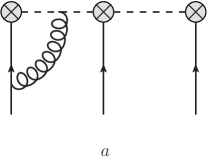
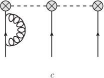
The $B$ operators, in (4.157), (4.158), satisfy the renormalization group equation that can be put into the form [154, 153]:

$$\mu\frac{d}{d\mu}B=\left(\mu\frac{\partial}{\partial\,\mu}+\beta(g)\frac{\partial}{\partial g}\right)\;B=\mathbb{H}\cdot B\;,$$ (4.159)

with $\mathbb{H}$ being the integral evolution operator [27]:

$$\mathbb{H}=-\frac{\alpha_{s}}{2\pi}\left[\left(1+1/N_{c}\right){\mathcal{H}}+3C_{F}/2\right];$$ (4.160)

and $\beta(g)$ standing for the QCD $\beta$-function. Here we employ the shortened notations of [27] in which the color factors and the trivial contributions of the self energy insertions are factored out. However, in Eq. (4.160) we restored the factor $-\frac{\alpha_{s}}{2\pi}$ that was not presented explicitly in Eq. (2.23) of Ref. [27]. The second term in (4.160), proportional to $C_{F}\equiv\frac{N_{c}^{2}-1}{2N_{c}}$, corresponds to the self-energy corrections of each quark field (see Fig. 19.c).

The operator ${\mathcal{H}}$ introduced in (4.160) acts in a different way on the chirality-$\frac{3}{2}$ operator (4.158) and on the chirality-$\frac{1}{2}$ operator (4.157).

• In the case of the chirality-$\frac{3}{2}$ operator (4.158), to one loop order accuracy, the operator ${\mathcal{H}}$ is determined by the vertex correction diagrams (see Fig. 19.a) corresponding to gluon exchanges between quark lines and gluons forming Wilson lines. According to calculations of Refs. [48, 154, 155] it reads:

  $${\mathcal{H}}_{3/2}={\mathcal{H}}^{v}_{1\,2}+{\mathcal{H}}^{v}_{2\,3}+{\mathcal{H}}^{v}_{1\,3}\;,$$ (4.161)

  where

  $${\mathcal{H}}^{v}_{1\,2}B(z_{1},z_{2},z_{3})=-\int_{0}^{1}\frac{d\alpha}{\alpha}\left\{\bar{\alpha}\left[B(z^{\alpha}_{1\,2},z_{2},z_{3})-B(z_{1},z_{2},z_{3})\right]\right.$$

  $$\left.+\bar{\alpha}\left[B(z_{1},z^{\alpha}_{2\,1},z_{3})-B(z_{1},z_{2},z_{3})\right]\right\}\;,$$ (4.162)

  with

  $$\bar{\alpha}\equiv 1-\alpha;\ \ \ z^{\alpha}_{i\,k}\equiv z_{i}\bar{\alpha}+z_{k}\alpha.$$ (4.163)

• In the case of the chirality-$\frac{1}{2}$ operator (4.157) the operator ${\mathcal{H}}$ is determined not only by the above contributions but also by those which correspond to Feynman diagrams with gluon exchange between quark lines having opposite chiralities (see Fig. 19 b). It can be written as

  $${\mathcal{H}}_{1/2}={\mathcal{H}}_{3/2}-{\mathcal{H}}^{e}_{1\,2}-{\mathcal{H}}^{e}_{2\,3}\;,$$ (4.164)

  where

  $${\mathcal{H}}^{e}_{1\,2}B(z_{1},z_{2},z_{3})=\int_{0}^{1}d_{3}\alpha\;B(z^{\alpha_{1}}_{1\,2},z^{\alpha_{2}}_{2\,1},z_{3})\;,$$ (4.165)

  with

  $$\int_{0}^{1}d_{3}\alpha\equiv\int_{0}^{1}d\alpha_{1}\,\int_{0}^{1}d\alpha_{2}\,\int_{0}^{1}d\alpha_{3}\,\delta(1-\alpha_{1}-\alpha_{2}-\alpha_{3})\;.$$ (4.166)

By performing the Taylor expansion of the generating functional at small distances one switches to the local operators

$$B\left(z_{1},z_{2},z_{3}\right)=\sum_{N}\sum_{n_{1}+n_{2}+n_{3}=N}\frac{z_{1}^{n_{1}}}{n_{1}!}\frac{z_{2}^{n_{2}}}{n_{2}!}\frac{z_{3}^{n_{3}}}{n_{3}!}(\overrightarrow{D}^{+})^{n_{1}}\Psi(0)(\overrightarrow{D}^{+})^{n_{2}}\Psi(0)(\overrightarrow{D}^{+})^{n_{3}}\Psi(0),$$ (4.167)

where $\overrightarrow{D}^{+}\equiv\overrightarrow{D}^{\mu}\,n_{\mu}$ is the covariant derivative (4.62). Since the total number of derivatives $N$ is invariant under the evolution equation (4.159), (4.160) takes a matrix form, with a square matrix of size $\frac{N(N+1)}{2}$ in a subspace corresponding to each given $N$.

The study of the evolution properties of TDAs can then be performed by considering hadronic matrix elements of the type

$$\langle A|\mathcal{O}_{\Psi}|B\rangle=\Psi\left(\partial_{1},\partial_{2},\partial_{3}\right)\langle A|B\left(z_{1},z_{2},z_{3}\right)|B\rangle\Big{|}_{z_{i}=0},$$ (4.168)

where $\Psi\left(\partial_{1},\partial_{2},\partial_{3}\right)$ is a certain derivative operator.

First we review an approach for solving the ERBL-type evolution equations of the baryon distribution amplitudes. It turns out to be convenient to reformulate this problem in the space of coefficient functions by representing the sums of monomials in (4.167)

$$\mathcal{O}=\sum_{n_{1}+n_{2}+n_{3}=N}c_{n_{1},n_{2},n_{3}}(\overrightarrow{D}^{+})^{n_{1}}\Psi(0)(\overrightarrow{D}^{+})^{n_{2}}\Psi(0)(\overrightarrow{D}^{+})^{n_{3}}\Psi(0)$$ (4.169)

by polynomials in three variables

$$\Psi\left(y_{1},y_{2},y_{3}\right)=\sum_{n_{1}+n_{2}+n_{3}=N}c_{n_{1}n_{2}n_{3}}y_{1}^{n_{1}}y_{2}^{n_{2}}y_{3}^{n_{3}}.$$ (4.170)

The problem of solving the evolution equation can be reduced to the eigenvalue problem

$$\mathcal{H}\cdot\Psi_{N,q}=\mathcal{E}_{N,q}\Psi_{N,q},$$ (4.171)

where for given $N$ the index $q$ refers to the number of the “energy level”. The eigenvalues $\mathcal{E}_{N,q}$ are in a direct correspondence with the anomalous dimensions:

$$\gamma_{N,q}\equiv\left(1+1/N_{c}\right)\mathcal{E}_{N,q}+3/2C_{F}.$$ (4.172)

In the next subsection we review the method of solving (4.171) based on the conformal partial wave expansion [27].

4.8.2 Conformal PW expansion for leading twist baryon DAs: basic definitions

The methods based on exploiting the conformal symmetry of the Lagrangian of massless QCD (see Ref. [156] for a review) turned out to be extremely efficient in solving the evolution Eqs. (4.171). The evolution operator $\mathcal{H}$ commutes with the generators of the conformal group. Therefore, the conformal symmetry strongly constrains the set of the eigenfunctions of the evolution operator. In the case of the two-body operator the conformal symmetry completely determines the solution of the evolution equations. However, in the case of three-body operators the conformal symmetry is not sufficient to uniquely determine the solution. It provides the solution up to an arbitrary function of one variable.

To take full advantage of the consequences of conformal symmetry for the general solution of Eq. (4.171) one decomposes the corresponding eigenfunctions over a suitable basis of conformal polynomials. There are several choices for conformal basis. For example, in Refs. [155] an expansion over the set of the Appell polynomials [157] was employed. However, a better suited basis was proposed in [27]. In the following we adopt this latter form of the conformal basis. The conformal expansion is performed with respect to the functions $\Psi^{(12)3}_{N,n}$:

$$\Psi^{(12)3}_{N,n}(y_{1},y_{2},y_{3})=(N+n+4)(y_{1}+y_{2})^{n}P_{N-n}^{(2n+3,1)}(y_{3}-y_{1}-y_{2})C_{n}^{\frac{3}{2}}\left(\frac{y_{1}-y_{2}}{y_{1}+y_{2}}\right).$$ (4.173)

Here $P_{N-n}^{(2n+3,1)}(\ldots)$ stand for the Jacobi polynomials and $C_{n}^{\frac{3}{2}}(\ldots)$ are the Gegenbauer polynomials [157].

The superscript $(12)3$ refers to the order in which the conformal spins of the three quarks are summed to form the total conformal spin $N+3$. First the conformal spins of the first and second quarks are summed to form the total conformal spin $n+2$, and then the conformal spin of the third quark is added. This order is of course arbitrary. The functions $\Psi^{(12)3}_{N,n}$, $\Psi^{1(23)}_{N,n}$ and $\Psi^{(31)2}_{N,n}$ are related with each other through the Racah-$6j$ symbols of the SL$(2)$ group:

$$\Psi^{(32)1}_{N,n}(y_{1},y_{2},y_{3})=(N+n+4)(y_{3}+y_{2})^{n}P_{N-n}^{(2n-3,1)}(y_{1}-y_{3}-y_{2})C_{n}^{\frac{3}{2}}\left(\frac{y_{3}-y_{2}}{y_{3}+y_{2}}\right)$$

$$=\sum_{0\leq n^{\prime}\leq N}\Omega_{nn^{\prime}}(N)\Psi^{(12)3}_{N,n^{\prime}}(y_{1},y_{2},y_{3}).$$ (4.174)

The explicit form of the matrices $\Omega_{nn^{\prime}}(N)$ and additional details can be found in Appendix B of Ref. [158].

The conformal basis (4.173) is normalized according to

$$\langle\Psi^{(12)3}_{N,n}|\Psi^{(12)3}_{M,m}\rangle$$

$$\equiv 120\int_{0}^{1}dy_{1}\int_{0}^{1}dy_{2}\int_{0}^{1}dy_{3}\delta(1-y_{1}-y_{2}-y_{3})y_{1}y_{2}y_{3}\Psi^{(12)3}_{N,n}(y_{1},y_{2},y_{3})\Psi^{(12)3}_{M,m}(y_{1},y_{2},y_{3})$$

$$=\delta_{MN}\delta_{mn}\frac{60}{2N+5}f_{N,n},$$ (4.175)

where $f_{N,n}=\frac{(n+1)(n+2)}{2(2n+3)}(N-n+1)(N+n+4).$

The conformal PW expansion of the leading twist-$3$ nucleon DA $\phi_{N}$ within the $(12)3$ basis (4.173) reads

$$\phi_{N}(y_{1},y_{2},y_{3})=120y_{1}y_{2}y_{3}\sum_{N=0}^{\infty}\sum_{n=0}^{N}\varphi_{N,n}^{(12)3}(\mu)\Psi^{(12)3}_{N,n}(y_{1},y_{2},y_{3});\ \ \ \ (y_{1}+y_{2}+y_{3}=1)\,.$$ (4.176)

The conformal moments in the conformal PW expansion (4.176) are defined as

$$\varphi_{N,n}^{(12)3}(\mu)$$

$$=\frac{2N+5}{60f_{N,n}}120\int_{0}^{1}dy_{1}\int_{0}^{1}dy_{2}\int_{0}^{1}dy_{3}\delta(1-y_{1}-y_{2}-y_{3})\Psi^{(12)3}_{N,n}(y_{1},y_{2},y_{3})\Phi(y_{1},y_{2},y_{3}).$$ (4.177)

To switch to a different basis (say $(31)2$) one makes use of the $\Omega_{nn^{\prime}}(N)$ matrix (4.174)

$$\varphi_{N,n}^{(31)2}(\mu)=\sum_{n^{\prime}=0}^{N}\Omega_{nn^{\prime}}(N)\varphi_{N,n}^{(12)3}(\mu).$$ (4.178)

The conformal invariance is not sufficient to resolve mixing of the coefficient $\varphi_{N,n}(\mu)$ with the same $N$ and different values of $n$. To diagonalize the mixing matrix and find the corresponding anomalous dimensions the advanced approach based on the complete integrability of the evolution equation for the baryon DAs with helicity-$\frac{3}{2}$ was proposed in [159, 27]. The numerical algorithms based on this approach were found extremely effective. This approach allows working out analytical expressions for corresponding eigenvalues and eigenvectors in the large-$N$ limit by means of a Wentzel–Kramers–Brillouin (WKB)-type expansion.

The multiplicatively renormalizable contributions to the nucleon DA (4.176) are given by linear combination of the conformal basis polynomials

$$P_{N,q}\left(y_{1},y_{2},y_{3}\right)=\sum_{n=0}^{N}c_{N,n}^{(q)}\Psi_{N,n}^{(12)3}\left(y_{1},y_{2},y_{3}\right),$$ (4.179)

where the coefficient $c_{N,n}^{(q)}$ can be found by diagonalization of the mixing matrix. The scale dependence of the leading twist-$3$ nucleon DA can be formally written as

$$\phi_{N}\left(y_{1},y_{2},y_{3},\mu^{2}\right)=y_{1}y_{2}y_{3}\sum_{N,\,q}\varphi_{N,q}P_{N,q}\left(y_{1},y_{2},y_{3}\right)\left(\frac{\alpha_{s}(\mu)}{\alpha_{s}\left(\mu_{0}\right)}\right)^{\gamma_{N,q}/b_{0}},$$ (4.180)

where $\gamma_{N,q}$ are the anomalous dimensions found from the solution of the eigenvalue problem (4.171) and $b_{0}=11/3N_{c}-2/3n_{f}$ is the first coefficient of the $\beta$-function of QCD. The coefficient $\varphi_{N,q}$ is scale-independent and can be seen as non-perturbative inputs.

4.8.3 Evolution equations for $\pi N$ TDAs

In this subsection we consider the derivation of the evolution equation for nucleon-to-meson TDAs. It repeats the main steps of the derivation of the evolution equations for GPDs [62]. The starting point is the renormalization group equation for the three-quark operator (4.159) with the evolution operator (4.160).

As a definite example we present the evolution equation for the combination of the leading twist-$2$ $\pi N$ TDAs (4.12)

$$T_{\uparrow\downarrow,\uparrow}^{\uparrow}(x_{1},x_{2},x_{3},\xi,\Delta^{2};\mu)\equiv T_{\uparrow\downarrow,\uparrow}^{\uparrow}(x_{i})\sim\left(V_{1}^{p\pi_{0}}(x_{i})-A_{1}^{p\pi_{0}}(x_{i})\right)$$ (4.181)

with $\pi N$ TDAs parameterized as in Eq. (4.4) with the set of Dirac structures (4.6).

The combination (4.181) is related to the matrix element of the three quark operator with the total chirality $\frac{1}{2}$ between a nucleon with chirality $\frac{1}{2}$ and a pion:

$$\langle\pi^{0}(p_{\pi})|\varepsilon^{c_{1}c_{2}c_{3}}(\hat{n}u_{c_{1}}^{\uparrow})_{\rho}(z_{1}n)(\hat{n}u_{c_{2}}^{\downarrow})_{\tau}(z_{2}n)(\hat{n}d_{c_{3}}^{\uparrow})_{\chi}(z_{3}n)|N^{\uparrow}(p_{N})\rangle.$$

The evolution equation takes the form [18]:

$$\mu\frac{d}{d\,\mu}\;T_{\uparrow\downarrow,\uparrow}^{\uparrow}(x_{i})=-\frac{\alpha_{s}}{2\pi}\left\{\frac{3}{2}\,C_{F}\,T_{\uparrow\downarrow,\uparrow}^{\uparrow}(x_{i})-\left(1+\frac{1}{N_{c}}\right)\right.$$ (4.182)

$$\left[\left(\int_{-1+\xi}^{1+\xi}dx_{1}^{\prime}\left[\frac{x_{1}\rho(x_{1}^{\prime},x_{1})}{x_{1}^{\prime}(x_{1}^{\prime}-x_{1})}\right]_{+}+\int_{-1+\xi}^{1+\xi}dx_{2}^{\prime}\left[\frac{x_{2}\rho(x_{2}^{\prime},x_{2})}{x_{2}^{\prime}(x_{2}^{\prime}-x_{2})}\right]_{+}\right)T_{\uparrow\downarrow,\uparrow}^{\uparrow}(x_{1}^{\prime},x_{2}^{\prime},x_{3})\right.$$

$$+\left(\int_{-1+\xi}^{1+\xi}dx_{1}^{\prime}\left[\frac{x_{1}\rho(x_{1}^{\prime},x_{1})}{x_{1}^{\prime}(x_{1}^{\prime}-x_{1})}\right]_{+}+\int_{-1+\xi}^{1+\xi}dx_{3}^{\prime}\left[\frac{x_{3}\rho(x_{3}^{\prime},x_{3})}{x_{3}^{\prime}(x_{3}^{\prime}-x_{3})}\right]_{+}\right)T_{\uparrow\downarrow,\uparrow}^{\uparrow}(x_{1}^{\prime},x_{2},x_{3}^{\prime})$$

$$+\left(\int_{-1+\xi}^{1+\xi}dx_{2}^{\prime}\left[\frac{x_{2}\rho(x_{2}^{\prime},x_{2})}{x_{2}^{\prime}(x_{2}^{\prime}-x_{2})}\right]_{+}+\int_{-1+\xi}^{1+\xi}dx_{3}^{\prime}\left[\frac{x_{3}\rho(x_{3}^{\prime},x_{3})}{x_{3}^{\prime}(x_{3}^{\prime}-x_{3})}\right]_{+}\right)T_{\uparrow\downarrow,\uparrow}^{\uparrow}(x_{1},x_{2}^{\prime},x_{3}^{\prime})$$

$$+\frac{1}{2\xi-x_{3}}\left(\int_{-1+\xi}^{1+\xi}dx_{1}^{\prime}\frac{x_{1}}{x_{1}^{\prime}}\rho(x_{1}^{\prime},x_{1})+\int_{-1+\xi}^{1+\xi}dx_{2}^{\prime}\frac{x_{2}}{x_{2}^{\prime}}\rho(x_{2}^{\prime},x_{2})\right)T_{\uparrow\downarrow,\uparrow}^{\uparrow}(x_{1}^{\prime},x_{2}^{\prime},x_{3})$$

$$\left.\left.+\frac{1}{2\xi-x_{1}}\left(\int_{-1+\xi}^{1+\xi}dx_{2}^{\prime}\frac{x_{2}}{x_{2}^{\prime}}\rho(x_{2}^{\prime},x_{2})+\int_{-1+\xi}^{1+\xi}dx_{3}^{\prime}\frac{x_{3}}{x_{3}^{\prime}}\rho(x_{3}^{\prime},x_{3})\right)T_{\uparrow\downarrow,\uparrow}^{\uparrow}(x_{1},x_{2}^{\prime},x_{3}^{\prime})\right]\right\}\;,$$

where $\left[\ldots\right]_{+}$ denotes the standard “$+$”-regularization prescription for generalized functions [143]:

$$\left[f\left(x,x^{\prime}\right)\right]_{+}=f\left(x,x^{\prime}\right)-\delta\left(x-x^{\prime}\right)\int dx^{\prime}f\left(x^{\prime},x^{\prime}\right).$$ (4.183)

The integration region in each integral is restricted in two ways. Firstly, the support of integrands is defined by functions $\rho(x,y)$

$$\rho(x,y)=\theta(x\geq y\geq 0)-\theta(x\leq y\leq 0),$$ (4.184)

with $\theta(x\geq y\geq 0)=\theta(x\geq y)\theta(y\geq 0)$. This function $\rho(x,y)$ is a generalization of the analogous one which appears in equations describing the pure ERBL evolution [62]. The second condition is the requirement that, although not denoted as a variable of integration, the variables $x^{\prime}_{i}$ must satisfy the condition $x^{\prime}_{i}\in[-1+\xi,1+\xi]$. For example, in the first integral over $x_{1}^{\prime}$ in the r.h.s. of (4.182) the variable $x_{2}^{\prime}=2\xi-x_{3}-x_{1}^{\prime}$ must belong to the interval $x_{2}^{\prime}\in[-1+\xi,1+\xi]$.

The evolution equation for the combination of TDAs (4.12) $T_{\uparrow\uparrow,\uparrow}^{\uparrow}(x_{i})\sim\left(T_{2}^{p\pi_{0}}(x_{i})-T_{3}^{p\pi_{0}}(x_{i})\right)$, that corresponds to the case where the three quarks have total chirality $3/2$, is obtained from (4.182) by neglecting the two last lines. The evolution equations for other TDA combinations listed in (4.12) can be obtained according to the same pattern.

It is worth emphasizing, that, similarly to the case of GPDs, the form of the evolution of nucleon-to-meson TDAs turns out to be different in various domains of the $x_{i}$ support.

• In particular, when all $x_{i}>0$ one is in the same kinematics as the usual ERBL equation for the baryons, with the simple $x_{i}\to x_{i}/2\xi$ rescaling. The solutions of Eq. (4.182) in the ERBL-like domain are thus well known and are expressed in terms of the conformal basis:

  $$H(x_{i},\xi,\mu^{2})=x_{1}x_{2}x_{3}\delta(x_{1}+x_{2}+x_{3}-2\xi)\sum_{N,q}h_{N,q}\,P_{N,q}(x_{i}/2\xi)\left(\frac{\alpha_{s}(\mu)}{\alpha_{s}(\mu_{0})}\right)^{\gamma_{n,q}/b_{0}},$$ (4.185)

  where $b_{0}=11/3N_{c}-2/3n_{f}$, $\gamma_{n,q}$ are the corresponding anomalous dimensions. The dimensionless parameters $h_{N,q}(\mu_{0})$ represent nonperturbative input for the evolution. They are to be fixed with the help of QCD sum rules technique or from lattice calculations.

• For the DGLAP-like domains, where one (or two) $x_{i}<0$, the solutions of the evolution Eqs. (4.182) are for the moment unknown and deserve further study.

4.8.4 Conformal partial wave expansion for nucleon-to-meson TDAs

GPD representations based on the conformal partial wave expansion were found to be a convenient tool both to address the fundamental properties of GPDs as well as for the phenomenological applications. The key advantages of this approach consist in a possibility to achieve the factorization of functional dependencies of GPDs on different variables and ensure diagonalization of the leading order (LO) evolution operator. It also provides a consistent framework to study evolution effects at NLO.

There are several versions of this formalism in the present day literature. In particular, the approach [160, 161, 162] relies on the Mellin–Barnes integral technique and the Sommerfeld–Watson transformation. This implies the analytic continuation of conformal moments and of conformal partial waves to the complex values of conformal spin.

An alternative approach is based on the so-called Shuvaev–Noritzsch transformation [163, 164]. A particular version of this formalism employing further expansion of conformal partial waves in terms of the cross-channel SO$(3)$ partial wave is known as the dual parametrization of GPDs [165, 166]. This latter picture makes a direct contact with a cross channel representation of GPDs as infinite sums of resonance exchanges with quantum numbers of mesons [135]. In Ref. [167] the dual parametrization of GPDs was found to be completely equivalent to the formalism based on the Mellin–Barnes integral techniques.

In this section we sketch a possible generalization of conformal PW expansion approach to the case of nucleon-to-meson TDAs. The conformal moments of nucleon-to-meson TDAs are formed with respect to the conformal basis (4.173). The corresponding polynomials take particularly simple form in terms of the quark–diquark coordinates (4.45). We employ the choice of quark–diquark coordinates (4.48). It is consistent with the order $(12)3$ in which the conformal spins of quark components are added up to form the total conformal spin $N+3$ of the three-quark operator. For simplicity in what follows we omit the subscript referring to the particular choice of quark–diquark coordinates: $w_{3}\equiv w$; $v_{3}\equiv v$; $\xi^{\prime}_{3}\equiv\xi^{\prime}$. The corresponding polynomials then read

$$\psi^{(12)3}_{N,n}(w,v,\xi)=\xi^{N}2^{N-n}(N+n-4)\left(1-\frac{w}{\xi}\right)^{n}C_{n}^{\frac{3}{2}}\left(\frac{v}{\xi^{\prime}}\right)P_{N-n}^{2n+3,1}\left(\frac{w}{\xi}\right).$$ (4.186)

The $(N,n)$-th conformal moments of a nucleon-to-meson TDA $H(w,v,\xi,\Delta^{2})$ $h_{N,n}^{(12)3}(\xi,\Delta^{2})$ are defined as integrals over the complete support domain of TDAs in quark–diquark coordinates (4.46):

$$h_{N,n}^{(12)3}(\xi,\Delta^{2})=\int_{-1}^{1}dw\int_{-1+|\xi-\xi^{\prime}|}^{1-|\xi-\xi^{\prime}|}dvH(w,v,\xi,\Delta^{2})\psi^{(12)3}_{N,n}(w,v,\xi).$$ (4.187)

We introduce the conformal PWs with the pure ERBL-like support (see Fig. 16):

$$p_{N,n}^{(12)3}(w,v,\xi)=\theta(-\xi\leq w\leq\xi)\,\theta(-\xi^{\prime}\leq v\leq\xi^{\prime})\,\xi^{-N-2}\frac{1}{g_{N,n}}$$

$$\times\left(1-\frac{v^{2}}{{\xi^{\prime}}^{2}}\right)C_{n}^{\frac{3}{2}}\left(-\frac{v}{\xi^{\prime}}\right)\left(1-\frac{w}{\xi}\right)^{n+2}\left(1+\frac{w}{\xi}\right)P_{N-n}^{2n+3,1}\left(\frac{w}{\xi}\right),$$ (4.188)

where $g_{N,n}$ is the convenient normalization factor

$$g_{N,n}=2^{N+n+5}\frac{(N-n+1)(n+1)(n+2)}{(2n+3)(2N+5)}.$$ (4.189)

The conformal basis (4.186) is normalized in a way that

$$\int_{-\xi}^{\xi}dw\int_{-\xi^{\prime}}^{\xi^{\prime}}dv\,p_{N,n}^{(12)3}(w,v,\xi)\,\psi^{(12)3}_{M,m}(w,v,\xi)=(-1)^{n}\delta_{MN}\delta_{mn}.$$ (4.190)

The conformal PW expansion for a nucleon-to-meson TDA can then be written as

$$H(w,v,\xi,\Delta^{2})=\sum_{N=0}^{\infty}\sum_{n=0}^{N}p_{N,n}^{(12)3}(w,v,\xi)h_{N,n}^{(12)3}(\xi,\Delta^{2})\,.$$ (4.191)

Due to the orthogonality relation (4.190), the series (4.191) reproduces the conformal moments of a TDA (4.187).

Since the conformal PWs (4.188) have only the ERBL-like support, this series must be seen as a representation of a TDA in the space of singular generalized functions. Similarly to the case of GPDs, the series (4.191) requires proper resummation in order to be defined rigorously in the mathematical sense. This turns to be a formidable problem that still awaits its complete solution.

A possible approach could be a generalization of the Mellin–Barnes integral technique that was efficiently employed in the GPD case. This requires the analytic continuation of both the conformal moments $h_{N,n}^{(12)3}$ and conformal PWs (4.188) to the complex values of the conformal spin of a $(12)$-quark pair $n+2$ and of the total conformal spin of the three-quark operator $N+3$. The Sommerfeld–Watson transformation can be employed to transform the formal series (4.191) into a double Mellin–Barnes type integral. The analytic continuation of the conformal PWs (4.188) can be performed with help of the familiar Schläfli integral representation for the Jacobi polynomials [168]:

$$P_{n}^{(\alpha,\beta)}(x)=\frac{2^{-n}}{2\pi i}\oint_{C}dz(z^{2}-1)^{n}\left(\frac{1-z}{1-x}\right)^{\alpha}\left(\frac{1+z}{1+x}\right)^{\beta}\frac{1}{(z-x)^{n+1}},$$ (4.192)

where $C$ is the usual contour making one counter-clockwise turn around $z=x$. Assuming the proper asymptotic behavior of the conformal moments $h_{N,n}^{(12)3}$ the uniqueness of the procedure can be ensured with help of the Carlson theorem [169].

However, the mathematical aspects of handling the double Mellin–Barnes-type integrals and symmetry issues related to switching between the equivalent $(12)3$, $(23)1$ and $(31)2$ conformal basis (c.f. Eq. (4.174)) still require further study. Also the intrinsic ambiguity of the analytic continuation of the anomalous dimensions of three-quark operators reported in [27] may signal possible severe complications for this approach.

Similarly to the GPD case, it is convenient to expand the conformal moments of TDAs over the partial waves of the cross-channel SO$(3)$ rotation group. For definiteness we consider the backward pion electroproduction reaction

$$\gamma^{*}(q)+N(p_{N})\to N^{\prime}(p^{\prime}_{N})+\pi(p_{\pi});$$ (4.193)

and its $u$-channel counterpart reaction

$$\gamma^{*}(q)+N^{\prime}(\tilde{p}^{\prime}_{N})\to N(\tilde{p}_{N})+\pi(p_{\pi}).$$ (4.194)

The crossing transformation, relating (4.194) to (4.193), reads

$$\tilde{p}^{\prime}_{N}\to-{p}^{\prime}_{N};\ \ \ \tilde{p}_{N}\to-{p}_{N};{}$$

$$s\big{|}_{\text{reaction (\ref{Cross_u_react})}}=(q+\tilde{p}^{\prime}_{N})^{2}\to u\big{|}_{\text{reaction (\ref{Direct_s_react})}}=(q-{p}^{\prime}_{N})^{2}.$$ (4.195)

Within the near-backward kinematics of Sec. 3.1 the cosine of the $u$-channel scattering angle of the reaction (4.193) can be expressed to the leading order in $1/Q$-expansion as

$$\cos\theta_{u}=-\frac{1-\xi\frac{m_{N}^{2}-m_{\pi}^{2}}{u}}{\xi\sqrt{1+\frac{(m^{2}_{N}-m_{\pi}^{2})^{2}}{{u}^{2}}-\frac{2(m_{N}^{2}+m_{\pi}^{2})}{u}}}+{\mathcal{O}}\left(\frac{1}{Q^{2}}\right)\,,$$ (4.196)

where $\xi$ is the $u$-channel skewness variable (3.14). Setting in (4.196) hadronic masses to zero corresponds to neglecting the $\pi N$ threshold corrections. This results in

$$\cos\theta_{u}\simeq-\frac{1}{\xi}.$$ (4.197)

To match with the polynomiality property of $\pi N$ TDAs (4.65), $h_{n,N}^{(12)3}(\xi,\Delta^{2})$ turn to be polynomials of $\xi$ of order $N+1$ for the TDAs $\{V_{1,2}^{\pi N},\,A_{1,2}^{\pi N},\,T_{1,2}^{\pi N}\}$ and of order $N$ for the $\{T_{3,4}^{\pi N}\}$ TDAs. Calculations of $N$ and $\Delta(1232)$ $u$-channel exchange contributions into $\pi N$ TDAs (see Sec. 5.1) provide insight on the proper cross-channel SO$(3)$ PW basis.

• For $H=\{V_{1,2}^{\pi N},\,A_{1,2}^{\pi N},\,T_{1,2}^{\pi N}\}$ TDAs the expansion goes over the Gegenbauer polynomials $P^{\prime}_{l+1}(1/\xi)=C_{l}^{\frac{3}{2}}(1/\xi):$

  $$h_{N,n}^{(12)3}(\xi,\Delta^{2})=\xi^{N+1}\sum_{l=0}^{N+1}B_{N,n,l}^{H}(\Delta^{2})C_{l}^{\frac{3}{2}}\left(\frac{1}{\xi}\right);$$ (4.198)

• For $H=\{T_{3,4}^{\pi N}\}$ TDAs the expansion goes over the Gegenbauer polynomials $P^{\prime}_{l}(1/\xi)=C_{l-1}^{\frac{3}{2}}(1/\xi):$

  $$h_{N,n}^{(12)3}(\xi,\Delta^{2})=\xi^{N}\sum_{l=0}^{N+1}B_{N,n,l}^{H}(\Delta^{2})C_{l-1}^{\frac{3}{2}}\left(\frac{1}{\xi}\right);$$ (4.199)

Here the generalized form factors $B_{N,n,l}^{H}(\Delta^{2})$ are functions of the invariant $u$-channel momentum transfer of the reaction (4.193) $\Delta^{2}=(p_{\pi}-p_{N})^{2}\equiv u$ and carry two conformal spin indices $N$, $n$ and the cross-channel SO$(3)$ rotation group index $l$.

Plugging (4.198), (4.199) into the conformal PW expansion (4.191) results in an analogue of the dual representation of GPDs for the case of nucleon-to-pion TDAs. Unfortunately, the summation of the corresponding formal series employing a generalization of methods of Ref. [165] has been only achieved for the limiting case $\xi=1$.

It is worth mentioning that the double (conformal and the cross-channel SO$(3)$) PW expansion for nucleon–pion GDAs/nucleon-to-pion TDAs arises naturally within the representation of corresponding matrix elements as infinite sums of the $u$-channel $N^{*}$- and $\Delta$-family resonance exchanges of arbitrary high half-integer spin and of arbitrary high mass (see Fig. 21).

Further development of the conformal partial wave expansion framework for the case of nucleon-to-meson (and nucleon-to-photon) TDAs is highly demanded, although mathematical difficulties considerably delay the progress. In particular, the calculation of the LO elementary amplitudes of hard processes (see Sec. LABEL:SubSec_Bkw_meson_ampl) within the conformal partial wave expansion framework for nucleon-to-meson TDAs still remains an open issue. Such studies are particularly interesting since, similarly to the case of GPD [170, 171, 144, 172], they can provide a new insight into the analytical properties of the LO elementary amplitudes. Also an adaptation for the case of TDAs of an analogue of the Regge-theory inspired Kumerički–Müller (KM) Ansatz for the conformal moments of GPDs [173] can be useful for phenomenological applications.

4.9 Nucleon-to-meson TDAs in impact parameter space

The use of the impact parameter representation to provide a vivid physical interpretation to GPDs and build up a comprehensible picture of hadrons in the transverse plane has been pioneered by M. Burkardt for GPDs in the zero skewness limit in Refs. [8, 174]. The extension of this framework for GPDs with non-zero skewness was proposed in Refs. [9, 10].

A possible novel physical aspect of nucleon-to-meson TDAs is their sensitivity to the effect of diquark clustering in hadrons [175, 176, 177, 178]. An attempt to study diquark clustering in light-cone functions (nucleon DA) and to provide dynamical explanation to the asymmetry of nucleon DA was performed in Ref. [179]. Below we consider a development of this idea. For this issue following Ref. [180] we address nucleon-to-meson TDAs integrated over quark–diquark coordinate $v_{i}$ (4.45). This provides access to hadronic matrix elements of a bilocal quark–diquark light-cone operator. Moreover, the general structure of integrated TDAs looks similar to GPDs and it is, therefore, natural to adopt for them the impact parameter space representation.

4.9.1 Integrated $\pi N$ TDAs and quark–diquark picture of the nucleon

For definiteness, we consider below the case of the proton ($N^{p}$)-to-$\pi^{0}$ $uud$ TDA (4.4). However, our results admit a straightforward generalization for other isospin channels for $\pi N$ TDAs as well as for more involved cases. In order to make contact to a quark–diquark picture we introduce $\pi N$ TDAs integrated over the momentum fraction variable $v_{i}$ (4.45). For definiteness in what follows we choose $i=3$ and employ the set of quark–diquark coordinates $w_{3}=x_{3}-\xi;\ \ v_{3}\equiv\frac{x_{1}-x_{2}}{2}$. The fraction of the longitudinal momentum carried by the first and second quarks is given by $x_{1}+x_{2}=2\xi_{3}^{\prime}$ with $\xi_{3}^{\prime}\equiv\frac{\xi-w_{3}}{2}$.

We integrate the definition (4.4) in $v_{3}$ over the interval $(-\infty;\,\infty)$:

$$\int_{-\infty}^{\infty}dv_{3}4{\mathcal{F}}\langle\pi^{0}(p_{\pi})|\,\widehat{O}_{\rho\tau\chi}^{\,uud}(\lambda_{1}n,\lambda_{2}n,\lambda_{3}n)\,|N^{p}(p_{N},s_{N})\rangle{}$$

$$=i\frac{f_{N}}{f_{\pi}}\Bigl{[}\sum_{\Upsilon=1,2}(v^{\pi N}_{\Upsilon})_{\rho\tau,\,\chi}\int_{-1+|\xi-\xi_{3}^{\prime}|}^{1-|\xi-\xi_{3}^{\prime}|}dv_{3}V_{\Upsilon}^{\pi N}(w_{3},v_{3},\xi,\Delta^{2})+\sum_{\Upsilon=1,\,2}(a^{\pi N}_{\Upsilon})_{\rho\tau,\,\chi}\int_{-1+|\xi-\xi_{3}^{\prime}|}^{1-|\xi-\xi_{3}^{\prime}|}dv_{3}A_{\Upsilon}^{\pi N}(w_{3},v_{3},\xi,\Delta^{2})$$

$$+\sum_{\Upsilon=1,2,3,4}(t^{\pi N}_{\Upsilon})_{\rho\tau,\,\chi}\int_{-1+|\xi-\xi_{3}^{\prime}|}^{1-|\xi-\xi_{3}^{\prime}|}dv_{3}T_{\Upsilon}^{\pi N}(w_{3},v_{3},\xi,\Delta^{2})\Bigr{]}.$$ (4.200)

In the r.h.s. of (4.200) the integral stands over the $v_{3}$ support (4.46) of $\pi N$ TDAs.

We employ the following identity for the exponent in the Fourier transform (4.5):

$${\mathcal{F}}(\ldots)=(P\cdot n)^{3}\int\left[\prod_{j=1}^{3}\frac{d\lambda_{j}}{2\pi}\right]e^{i(\frac{x_{1}-x_{2}}{2}(\lambda_{1}-\lambda_{2})+\frac{x_{1}+x_{2}}{2}(\lambda_{1}+\lambda_{2})+x_{3}\lambda_{3})P\cdot n}{}$$

$$\equiv(P\cdot n)^{3}\int\left[\prod_{j=1}^{3}\frac{d\lambda_{j}}{2\pi}\right]e^{i(v_{3}(\lambda_{1}-\lambda_{2})+\xi_{3}^{\prime}(\lambda_{1}+\lambda_{2})+x_{3}\lambda_{3})P\cdot n}.$$ (4.201)

In the l.h.s. of (4.200) the integration of the exponent (4.201) results in the delta function $\delta(\lambda_{1}-\lambda_{2})$, which allows to remove one of the $\lambda_{j}$-integrals. Finally, this brings the arguments of the two $u$-quark operators to the same point on the light cone $\lambda_{1}n=\lambda_{2}n\equiv\lambda_{D}n$ and gives rise to the hadronic matrix element of a bilocal light-cone operator:

$$\widehat{O}_{\rho\tau\chi}^{\{uu\}d}(\lambda_{D}n,\lambda_{D}n,\lambda_{3}n)=u_{\rho}(\lambda_{D}n)u_{\tau}(\lambda_{D}n)d_{\chi}(\lambda_{3}n)\equiv\widehat{D}_{\rho\tau}^{uu}(\lambda_{D}n)d_{\chi}(\lambda_{3}n).$$ (4.202)

It is natural to interpret (4.202) as the bilocal $uu$-diquark- $d$-quark operator on the light-cone. Now we employ the translation invariance of the matrix element to shift the arguments of the bilocal operator (4.202) to the symmetric points $\pm\frac{\lambda}{2}$ on the light-cone introducing $\lambda\equiv\lambda_{3}-\lambda_{D}$ and $\mu\equiv\lambda_{3}+\lambda_{D}$. The integral over $\mu$ can be performed producing the momentum conservation $\delta$-function:

$$\int\frac{d\mu}{2\pi}e^{i\left(x_{D}+x_{3}-2\xi\right)(P\cdot n)2\mu}=\frac{1}{2(P\cdot n)}\delta(x_{D}+x_{3}-2\xi);\ \ \ x_{D}\equiv x_{1}+x_{2}=2\xi^{\prime}_{3}.$$ (4.203)

Finally, we get the equality relating the Fourier transform of the nucleon–pion matrix element of the light-cone diquark–quark operator (4.202) to the $v_{3}$-integrated nucleon-to-pion TDAs:

$$2(P\cdot n)\int\frac{d\lambda}{4\pi}e^{i\left(w_{3}\lambda\right)(P\cdot n)}\langle\pi(p_{\pi})|\widehat{D}_{\rho\tau}^{\,uu}(-\frac{\lambda}{2}n){d}_{\chi}(\frac{\lambda}{2}n)|N(p_{N})\rangle{}$$

$$=i\frac{f_{N}}{f_{\pi}}\Bigl{[}\sum_{\Upsilon=1,2}(v^{\pi N}_{\Upsilon})_{\rho\tau,\,\chi}\int_{-1+|\xi-\xi_{3}^{\prime}|}^{1-|\xi-\xi_{3}^{\prime}|}dv_{3}V_{\Upsilon}^{\pi N}(w_{3},v_{3},\xi,\Delta^{2})+\sum_{\Upsilon=1,\,2}(a^{\pi N}_{\Upsilon})_{\rho\tau,\,\chi}\int_{-1+|\xi-\xi_{3}^{\prime}|}^{1-|\xi-\xi_{3}^{\prime}|}dv_{3}A_{\Upsilon}^{\pi N}(w_{3},v_{3},\xi,\Delta^{2})$$

$$+\sum_{\Upsilon=1,2,3,4}(t^{\pi N}_{\Upsilon})_{\rho\tau,\,\chi}\int_{-1+|\xi-\xi_{3}^{\prime}|}^{1-|\xi-\xi_{3}^{\prime}|}dv_{3}T_{\Upsilon}^{\pi N}(w_{3},v_{3},\xi,\Delta^{2})\Bigr{]}.$$ (4.204)

The $v_{3}$-integrated TDAs occurring in the r.h.s. of Eq. (4.204) share many common features with GPDs:

• They are functions of one longitudinal momentum fraction $w_{3}=\frac{x_{3}-x_{D}}{2}\in[-1;\,1]$, of skewness $\xi$, of the invariant momentum transfer $\Delta^{2}$ (and of the factorization scale).

• As a consequence of the Lorentz invariance, the Mellin moments of $v_{3}$-integrated TDAs possess the usual polynomiality property in $\xi$.

• For the $v_{3}$-integrated TDAs it is natural to specify the ERBL-region with $w_{3}\in[-\xi;\xi]$, DGLAP-I region $w_{3}\in[-1;\,-\xi]$ and DGLAP-II region $w_{3}\in[\xi;\,1]$.

A complementary picture can be obtained from the $\pi N$ TDAs integrated over $v_{1}=\frac{x_{2}-x_{3}}{2}$. This results in a $\pi N$ matrix element of a quark–diquark operator

$$\widehat{O}_{\rho\tau\chi}^{u\{ud\}}(\lambda_{1}n,\lambda_{D}n,\lambda_{D}n)=u_{\rho}(\lambda_{1}n)u_{\tau}(\lambda_{D}n)d_{\chi}(\lambda_{D}n)\equiv\widehat{D}_{\tau\chi}^{ud}(\lambda_{D}n)u_{\rho}(\lambda_{1}n).$$ (4.205)

with a diquark constructed out of the third and second quarks ($du$). In this case, the Dirac structures in the r.h.s. of the analogue of Eq. (4.204) must be Fierz transformed (see App. LABEL:App_Fierz) to get the appropriate order of the Dirac indices (first two indices correspond to a diquark):

$$\{v^{\pi N}_{\Upsilon},\,a^{\pi N}_{\Upsilon},\,t^{\pi N}_{\Upsilon}\}_{\rho\tau,\,\chi}\to\{v^{\pi N}_{\Upsilon},\,a^{\pi N}_{\Upsilon},\,t^{\pi N}_{\Upsilon}\}_{\tau\chi,\,\rho}.$$

Such transformation produces certain combinations of $v_{1}$-integrated $\pi N$ TDAs at the Dirac structures $\{v^{\pi N}_{\Upsilon},\,a^{\pi N}_{\Upsilon},\,t^{\pi N}_{\Upsilon}\}_{\tau\chi,\,\rho}$.

Finally, the third complementary picture results from $v_{2}$-integrated TDAs defined by the $\pi N$ matrix element of a quark–diquark operator

$$\widehat{O}_{\rho\tau\chi}^{\{u\check{u}d\}}(\lambda_{D}n,\lambda_{2}n,\lambda_{D}n)=u_{\rho}(\lambda_{D}n)u_{\tau}(\lambda_{2}n)d_{\chi}(\lambda_{D}n)\equiv\widehat{D}_{\rho\chi}^{ud}(\lambda_{D}n)u_{\tau}(\lambda_{2}n)$$ (4.206)

with a $ud$-diquark constituted of the first ($u$) and third ($d$) quarks.

4.9.2 Integrated TDAs in impact parameter space

We now propose an interpretation of the $v$-integrated TDAs in the impact parameter space. It allows us to use these objects as a tool to study the quark–diquark structure of hadrons in the transverse plane. It is worth emphasizing that, contrary to GPDs, the $v$-integrated TDAs do not possess a comprehensible forward limit in which a probabilistic interpretation [8, 174] applies for GPDs. Thus, similarly to the case of GPDs with non-zero skewness, we seek for an interpretation in terms of probability amplitudes.

The first step consists in introducing the initial nucleon and final meson states with specified longitudinal momenta localized around a definite position ${\mathbf{b}}$ in the transverse plane:

$$|p_{N}^{+},\,{\mathbf{b}};\,s_{N}\rangle=\int\frac{d^{2}{\mathbf{p}}_{N}}{16\pi^{3}}e^{-i{\mathbf{p}}_{N}\cdot{\mathbf{b}}}|p_{N}^{+},\,{\mathbf{p}}_{N};\,s_{N}\rangle;\ \ \ \langle p_{\pi}^{+},\,{\mathbf{b}}|=\int\frac{d^{2}{\mathbf{p}}_{\pi}}{16\pi^{3}}e^{i{\mathbf{p}}_{\pi}\cdot{\mathbf{b}}}\langle p_{\pi}^{+},\,{\mathbf{p}}_{\pi}|.$$ (4.207)

Rigorous treatment requires forming wave packets with precisely localized states (4.207) using a smooth weight falling sufficiently fast at infinity with $|{\mathbf{p}}|$ in order to avoid infinities due to normalization. A possible choice is to employ Gaussian wave packets with the same standard deviation parameter for the initial nucleon and the final meson.

Switching to the impact parameter space representation is performed by Fourier transforming the corresponding operator hadronic matrix element with respect to the transverse component ${\mathbf{D}}$ of the vector $D$:

$$D=\frac{p_{\pi}}{1-\xi}-\frac{p_{N}}{1+\xi}.$$ (4.208)

By construction, the transverse component ${\mathbf{D}}$ is invariant under the transverse boosts

$$k^{+}\to k^{+};\ \;{\mathbf{k}}\to{\mathbf{k}}-k^{+}{\mathbf{v}}.$$

This ensures that the invariant momentum transfer depends on ${\mathbf{p}}_{N}$ and ${\mathbf{p}}_{\pi}$ only through ${\mathbf{D}}$:

$$\Delta^{2}=-2\xi\left(\frac{m_{\pi}^{2}}{1-\xi}-\frac{m_{N}^{2}}{1+\xi}\right)-(1-\xi^{2}){\mathbf{D}}^{2}.$$ (4.209)

We consider the matrix elements of the diquark–quark operator with an explicit dependence on the transverse position ${\mathbf{z}}$:

$${\widehat{\mathcal{O}}}_{\rho\tau\chi}^{\{uu\}d}({{\mathbf{z}}})=\int\frac{d\lambda}{4\pi}e^{i\left(w_{3}\lambda\right)(P\cdot n)}{u}_{\rho}(0,\,-\frac{\lambda}{2},\,{\mathbf{z}}){u}_{\tau}(0,\,-\frac{\lambda}{2},\,{\mathbf{z}}){d}_{\chi}(0,\,\frac{\lambda}{2},\,{\mathbf{z}}),$$ (4.210)

where we adopt the following convention for the position arguments of quark fields: $q(z)=q(z^{+},\,z^{-},\,{\mathbf{z}})$.

In order to single out a particular combination of $\pi N$ TDAs we contract the matrix element of the operator (4.210) over the Dirac indices with a suitable projector. Assuming that for $\pi N$ TDAs we employ the parametrization of Eq. (10) of Ref. [40] we, as an example, have chosen to contract the matrix element (4.210) with $v^{-1}_{\tau\rho,\,\chi}=\left(C^{-1}\hat{P}\right)_{\tau\rho}\bar{U}_{\chi}(p_{N},s_{N}).$ Since we deal with unpolarized nucleon, we sum and average over the nucleon spin $s_{N}$. This convolution singles out the following combination of $v_{3}$-integrated $\pi N$ TDAs:

$${\mathcal{H}}^{\pi N}(w_{3},\,\xi,\,{\mathbf{D}})=(4m_{N}^{2}-\Delta^{2})\int_{-1+|\xi-\xi^{\prime}_{3}|}^{1-|\xi-\xi^{\prime}_{3}|}dv_{3}\frac{1}{2}\Bigl{[}(3m_{N}^{2}+m_{\pi}^{2}-\Delta^{2})V_{1}^{\pi N}(w_{3},\,v_{3},\,\xi,\,\Delta^{2}){}$$

$$+(-2\Delta^{2}-2m_{N}^{2}+2m_{\pi}^{2})V_{2}^{\pi N}(w_{3},\,v_{3},\,\xi,\,\Delta^{2})\Bigr{]},$$ (4.211)

where $\Delta^{2}$ is expressed through ${\mathbf{D}}^{2}$. The contraction with different projectors will allow to single out other combinations of $8$ leading twist-$3$ proton-to-$\pi^{0}$ $uud$ TDAs. The transition to the impact parameter space then gives

$$\int\frac{d^{2}{\bf D}}{(2\pi)^{2}}\;e^{-i\,{\mathbf{D}}\cdot{\mathbf{b}}}\,{\mathcal{H}}^{\pi N}(w,\xi,{\mathbf{D}})$$

$$={\mathcal{N}}^{-1}\frac{1+\xi^{2}}{(1-\xi^{2})^{2}}\>\;\sum_{s_{N}}\left(C^{-1}\hat{P}\right)_{\tau\rho}\bar{U}_{\chi}(p_{N};\,s_{N})\langle p_{\pi}^{+},-\frac{\xi{\mathbf{b}}}{1-\xi}\,\big{|}\,{\widehat{\mathcal{O}}}_{\rho\tau\chi}^{\{uu\}d}({{\mathbf{b}}})\,\big{|}\,p^{+}_{N},\frac{\xi{\mathbf{b}}}{1+\xi};\,s_{N}\rangle\;,$$ (4.212)

where $\mathcal{N}$ is a normalization factor originating from the normalization of the localized states (4.207). Without use of smooth wave packets it would be singular as $\delta^{(2)}({\bf 0})$.

We end up with a picture that is completely analogous to the GPD case (see Fig. 4): the hard probe interacts with a partonic configuration at the transverse position ${\mathbf{b}}$. The initial state nucleon and the finite state meson are localized around ${\bf 0}$, but they are shifted one from another by a transverse separation of the order $\xi{\mathbf{b}}$. This interpretation is presented in Fig. 20. It is also qualitatively consistent with the low Fock component picture proposed in [129], see Sec. 5.3.

• In the DGLAP-like I region $w_{3}\leq-\xi$ the impact parameter specifies the location where a $uu$-diquark is pulled out of a proton and then replaced by an antiquark $\bar{d}$ to form the final state meson.

• In the DGLAP-like II region $w_{3}\geq\xi$ the impact parameter specifies the location where a quark $d$ is pulled out of a proton and then replaced by an antidiquark $\bar{u}\bar{u}$ to form the final state meson.

• In the ERBL-like region $-\xi\leq w_{3}\leq\xi$ the impact parameter specifies the location where a three-quark cluster composed of a $uu$-diquark and a $d$-quark is pulled out of the initial nucleon to form the final state meson.

Figure 20: Impact parameter space interpretation for the $v_{3}$-integrated $uud$ $\pi N$ TDA in the DGLAP-like I, DGLAP-like II and in the ERBL-like domains. Solid arrows show the direction of the positive longitudinal momentum flow.

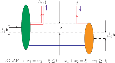
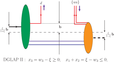
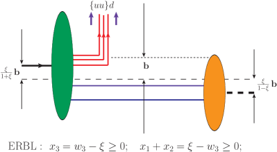
5 Dynamics and models

In this section we review the existing approaches for modeling nucleon-to-meson TDAs.

5.1 Cross-channel baryon exchange contributions

Cross-channel meson exchange contributions to GPDs were extensively applied to GPD phenomenology [95, 181]. In the left panel of Fig. 21 we show the pion exchange contribution that was found substantial for the nucleon polarized GPD $\tilde{E}^{u-d}$, see Ref. [182].

Similarly to the case of GPDs, cross-channel hadron exchange contributions provide a useful estimate for nucleon-to-meson TDAs. The corresponding hadrons possess quantum numbers of baryons. The relevant diagram is depicted in the right panel of Fig. 21. For unflavored meson the lightest possible baryon occurring in the cross channel is obviously a nucleon. The problem of eventual non-negligible corrections due to an analytic continuation from $\Delta^{2}\sim m_{N}^{2}$ to the values of $\Delta^{2}$ typical for the direct channel reaction has the same status as for the case of GPDs.

In this subsection we review the cross-channel nucleon exchange contributions into nucleon-to-pion and nucleon-to-vector-meson TDAs. We also consider a more involved $\Delta(1232)$-exchange contribution into nucleon-to-pion TDAs.

Figure 21: Left: pion-exchange model for the nucleon polarized GPD $\tilde{E}$; lower and upper blobs depict pion DAs; the dashed circle contains a typical LO graph for the pion electromagnetic form factor in perturbative QCD; the rectangle contains the pion pole contribution into GPD $\tilde{E}$. Right: cross-channel baryon exchange model for ${\mathcal{M}}N$ TDAs; dashed circle contains a typical LO graph for the baryon electromagnetic form factor in perturbative QCD; the rectangle contains the cross channel baryon contribution into ${\mathcal{M}}N$ TDAs

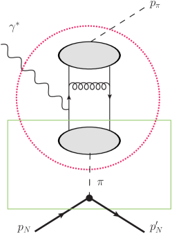
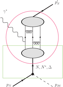
5.1.1 Cross-channel nucleon exchange contribution for $\pi N$ TDAs

Cross-channel nucleon exchange contribution to $\pi N$ TDAs corresponds to the lower part of the graph depicted in the right panel of Fig. 21. For the effective $\pi\bar{N}N$ interaction vertex we employ the standard parametrization (see e.g. [150])

$$\mathcal{V}_{\rm eff}(\pi NN)=ig_{\pi NN}\bar{N}_{\alpha}(\sigma_{a})^{\alpha}_{\;\beta}\gamma_{5}N^{\beta}\pi_{a}\,,$$ (5.1)

where $g_{\pi NN}\simeq 13$ is the nucleon–pion dimensionless coupling constant [183].

After reduction, the matrix element corresponding to the diagram in question reads:

$$\langle\pi_{a}(p_{\pi})|\widehat{O}^{\alpha\,\beta\,\gamma}_{\rho\tau\chi}(\lambda_{1}n,\,\lambda_{2}n,\,\lambda_{3}n)|N_{\iota}(p_{1},s_{1})\rangle$$

$$=\sum_{s_{p}}\langle 0|\widehat{O}^{\alpha\beta\gamma}_{\rho\tau\chi}(\lambda_{1}n,\,\lambda_{2}n,\,\lambda_{3}n)|N_{\kappa}(-\Delta,s_{p})\rangle(\sigma_{a})^{\kappa}_{\ \ \iota}\frac{ig_{\pi NN}\,\bar{U}_{\varrho}(-\Delta,s_{p})}{\Delta^{2}-m_{N}^{2}}\left(\gamma^{5}U(p_{1},s_{1})\right)_{\varrho}\,.$$ (5.2)

The operator matrix element in the second line of (5.2) is expressed through the leading twist-$3$ nucleon DAs by means of the inverse Fourier transform

$$\mathcal{F}^{-1}(\lambda_{k}(-\Delta\cdot n))(...)=\int d^{3}y\delta(1-y_{1}-y_{2}-y_{3})e^{i(p\cdot n)2\xi\sum_{k=1}^{3}y_{k}\lambda_{k}}(...)\,.$$ (5.3)

Following that, $\pi N$ TDAs are computed from the matrix element (5.2) by the Fourier transform (4.5) with help of the master formula

$$4\mathcal{F}(x_{1},x_{2},x_{3})\frac{1}{4}\bigl{[}\mathcal{F}^{-1}(\lambda_{k}(-\Delta\cdot n))\bigl{[}M^{N\,\{12\}}_{\rho\tau\chi}(y_{1},\,y_{2},\,y_{3})\bigr{]}\bigr{]}$$

$$=(p\cdot n)^{3}\int_{0}^{1}dy_{1}dy_{2}dy_{3}\delta(1-y_{1}-y_{2}-y_{3})\bigl{[}\prod_{k=1}^{3}\frac{1}{2\pi}\int d\lambda_{k}e^{i\lambda_{k}(x_{k}-2\xi y_{k})(p\cdot n)}\bigr{]}M^{N\,\{12\}}_{\rho\tau\chi}(y_{1},\,y_{2},\,y_{3})$$

$$=\frac{1}{(2\xi)^{2}}\delta(x_{1}+x_{2}+x_{3}-2\xi)\,\Theta_{\rm ERBL}(x_{1},x_{2},x_{3})\,M^{N\,\{12\}}_{\rho\tau\chi}\left(\frac{x_{1}}{2\xi},\frac{x_{2}}{2\xi},\frac{x_{3}}{2\xi}\right)\,,$$ (5.4)

where we employ the notation

$$\Theta_{\rm ERBL}(x_{1},x_{2},x_{3})\equiv\prod_{k=1}^{3}\theta(0\leq x_{k}\leq 2\xi)\,.$$ (5.5)

Obviously, the cross-channel nucleon exchange contributes only into the isospin-$\frac{1}{2}$ $\pi N$ TDAs. One can establish the following expressions for the set of invariant $\pi N$ TDAs defined in Sec. 4.4:

$$\bigl{\{}V_{1},\,A_{1},\,T_{1}\bigr{\}}^{(\pi N)_{1/2}}(x_{1},x_{2},x_{3},\xi,\Delta^{2})\Big{|}_{N(940)}$$

$$=\Theta_{\rm ERBL}(x_{1},x_{2},x_{3})\times(g_{\pi NN})\frac{m_{N}f_{\pi}}{\Delta^{2}-m_{N}^{2}}2\xi\frac{1}{(2\xi)^{2}}\bigl{\{}V^{p},\,A^{p},\,T^{p}\bigr{\}}\left(\frac{x_{1}}{2\xi},\frac{x_{2}}{2\xi},\frac{x_{3}}{2\xi}\right);$$

$$\bigl{\{}V_{2},\,A_{2},\,T_{2}\bigr{\}}^{(\pi N)_{1/2}}(x_{1},x_{2},x_{3},\xi,\Delta^{2})\Big{|}_{N(940)}=\frac{1}{2}\bigl{\{}V_{1},\,A_{1},\,T_{1}\bigr{\}}^{(\pi N)_{1/2}}(x_{1},x_{2},x_{3},\xi,\Delta^{2})\Big{|}_{N(940)};$$

$$\bigl{\{}T_{3},\,T_{4}\bigr{\}}^{(\pi N)_{1/2}}(x_{1},x_{2},x_{3},\xi,\Delta^{2})\Big{|}_{N(940)}=0,$$ (5.6)

where $V^{p}(y_{1},y_{2},y_{3})$, $A^{p}(y_{1},y_{2},y_{3})$ and $T^{p}(y_{1},y_{2},y_{3})$ stand for the usual leading twist-$3$ nucleon DAs [146].

The isotopic factors for the cross-channel nucleon exchange contributions for $p\to\pi^{0}$ $uud$, $n\to\pi^{-}$ $uud$ and $p\to\pi^{+}$ $ddu$ TDAs can be read off Eqs. (4.124), (4.125).

Note that (5.6) is a pure $D$- term like contribution. It is nonzero only in the ERBL-like region and its $(n_{1},n_{2},n_{3})$-th ($n_{1}+n_{2}+n_{3}=N$) Mellin moments (4.65) give rise to monomials of $\xi$ of the maximal possible power $N+1$.

The cross-channel nucleon exchange TDA model can be easily generalized for the case of different species of pseudoscalar mesons ($\eta$, $\eta^{\prime}$, etc.). The corresponding coupling constants with nucleons can be found e.g. in Ref. [184].

5.1.2 $\Delta(1232)$ exchange contribution for $\pi N$ TDAs

In this subsection we present the explicit expressions for $\Delta(1232)$ exchange contribution to $\pi N$ TDAs. The $\Delta$-exchange complements the nucleon exchange contribution presented in Sec. 5.1.1 and contributes to the isospin-$\frac{3}{2}$ $\pi N$ TDAs. In particular, the $\Delta$-exchange gives a non-trivial contribution to the least known $\pi N$ TDAs $T_{3,\,4}^{\pi N}$.

The effective vertex for the $\Delta N\pi$ interaction reads (see e.g. [147]):

$$\mathcal{V}_{\rm eff}(\pi N{\Delta})=g_{\pi N{\Delta}}\overline{N}_{\kappa}\,{P^{I=\frac{3}{2}}}_{ba\iota}^{\;\kappa}R_{\mu\,a}^{\,\iota}\,\partial^{\mu}\pi_{b}+{\rm h.c.},$$ (5.7)

where $R_{\mu\,a}^{\,\iota}$ is the Rarita–Schwinger spin-tensor describing spin-$\frac{3}{2}$ resonance field. It is contracted with the $P^{I=\frac{3}{2}}$ isospin-$\frac{3}{2}$ projecting operator (4.111). $g_{\pi N{\Delta}}$ is a dimensional coupling constant. Computation from the PDG [185] average ${\Delta(1232)}\rightarrow\pi N$ decay width gives: $|g_{\pi N{\Delta}}|\approx 7.6\ \;{\rm GeV}^{-1}\,.$

After the reduction the matrix element corresponding to the cross-channel $\Delta$-exchange contribution into $\pi N$ TDAs (see Fig. 21) reads:

$$\langle\pi_{a}(p_{\pi})|\widehat{O}^{\alpha\beta\gamma}_{\rho\tau\chi}(1,\,2,\,3)|N_{\iota}(p_{1},s_{1})\rangle$$

$$=\sum_{s_{\Delta}}\langle 0|\widehat{O}^{\alpha\beta\gamma}_{\rho\tau\chi}(1,\,2,\,3)|\Delta_{b\kappa}(-\Delta,s_{\Delta})\rangle{P^{I=\frac{3}{2}}}^{\;\;\kappa}_{b\ \ a\iota}\frac{g_{\pi N\Delta}\,\bar{\mathcal{U}}_{\varrho}^{\nu}(-\Delta,s_{\Delta})}{\Delta^{2}-m_{\Delta}^{2}}(iP_{\nu})\left(U(p_{1},s_{1})\right)_{\varrho}\,,$$ (5.8)

where $\mathcal{U}^{\nu}_{\varrho}$ is the Rarita–Schwinger spin-tensor describing the $\Delta$ resonance. For the matrix element involving $\Delta$ in the second line of (5.8) we employ the parametrization (4.112) with $M^{\Delta}_{\rho\tau\chi}$ given by (4.115). As a consequence of the identity (4.114) the cross-channel $\Delta$-exchange populates only the isospin-$\frac{3}{2}$ $\pi N$ TDAs.

Below, to the leading twist-$3$ accuracy, we present the contribution of (5.8) into the invariant $\pi N$ TDAs using the fully covariant parametrization of Sec. 4.4.

$$\left\{V_{1,2}^{(\pi N)_{3/2}},\,A_{1,2}^{(\pi N)_{3/2}}\right\}(x_{1},x_{2},x_{3},\xi,\Delta^{2})\Big{|}_{\Delta(1232)}$$

$$=-\Theta_{\rm ERBL}(x_{1},x_{2},x_{3})\frac{1}{(2\xi)^{2}}\left\{V^{\Delta},\,A^{\Delta}\right\}\left(\frac{x_{1}}{2\xi},\frac{x_{2}}{2\xi},\frac{x_{3}}{2\xi}\right)\frac{g_{\pi N\Delta}\lambda_{\Delta}^{\frac{1}{2}}m_{N}f_{\pi}}{\sqrt{2}(\Delta^{2}-m_{\Delta}^{2})f_{N}}\;R_{1,2}(\xi,m_{\Delta})\,;$$ (5.9)

$$T_{1}^{(\pi N)_{3/2}}(x_{1},x_{2},x_{3},\xi,\Delta^{2})\Big{|}_{\Delta(1232)}$$

$$=-\Theta_{\rm ERBL}(x_{1},x_{2},x_{3})\Bigm{\{}\frac{1}{(2\xi)^{2}}T^{\Delta}\left(\frac{x_{1}}{2\xi},\frac{x_{2}}{2\xi},\frac{x_{3}}{2\xi}\right)\frac{g_{\pi N\Delta}\lambda_{\Delta}^{\frac{1}{2}}m_{N}f_{\pi}}{\sqrt{2}f_{N}(\Delta^{2}-m_{\Delta}^{2})}R_{1}(\xi,m_{\Delta})$$

$$+\frac{1}{(2\xi)^{2}}\phi^{\Delta}\left(\frac{x_{1}}{2\xi},\frac{x_{2}}{2\xi},\frac{x_{3}}{2\xi}\right)\frac{g_{\pi N\Delta}f_{\Delta}^{\frac{3}{2}}m_{N}^{2}f_{\pi}}{\sqrt{2}f_{N}}\left(\frac{\widetilde{R}_{1}(\xi,m_{\Delta})}{\Delta^{2}-m_{\Delta}^{2}}-\frac{1-\xi}{2m_{N}^{2}}\right)\Bigm{\}}\,;$$ (5.10)

$$T_{2}^{(\pi N)_{3/2}}(x_{1},x_{2},x_{3},\xi,\Delta^{2})\Big{|}_{\Delta(1232)}$$

$$=-\Theta_{\rm ERBL}(x_{1},x_{2},x_{3})\Bigl{\{}\frac{1}{(2\xi)^{2}}T^{\Delta}\left(\frac{x_{1}}{2\xi},\frac{x_{2}}{2\xi},\frac{x_{3}}{2\xi}\right)\frac{g_{\pi N\Delta}\lambda_{\Delta}^{\frac{1}{2}}m_{N}f_{\pi}}{\sqrt{2}f_{N}(\Delta^{2}-m_{\Delta}^{2})}R_{2}(\xi,m_{\Delta})$$

$$+\frac{1}{(2\xi)^{2}}\phi^{\Delta}\left(\frac{x_{1}}{2\xi},\frac{x_{2}}{2\xi},\frac{x_{3}}{2\xi}\right)\frac{g_{\pi N\Delta}f_{\Delta}^{\frac{3}{2}}m_{N}^{2}f_{\pi}}{\sqrt{2}f_{N}}\left(\frac{\widetilde{R}_{2}(\xi,m_{\Delta})}{\Delta^{2}-m_{\Delta}^{2}}+\frac{1-\xi}{4m_{N}^{2}}\right)\Bigr{\}}\,;$$ (5.11)

$$T_{3,4}^{(\pi N)_{3/2}}(x_{1},x_{2},x_{3},\xi,\Delta^{2})\Big{|}_{\Delta(1232)}$$

$$=-\Theta_{\rm ERBL}(x_{1},x_{2},x_{3})\frac{1}{(2\xi)^{2}}\phi^{\Delta}\left(\frac{x_{1}}{2\xi},\frac{x_{2}}{2\xi},\frac{x_{3}}{2\xi}\right)\times\frac{g_{\pi N\Delta}f_{\Delta}^{\frac{3}{2}}m_{N}^{2}f_{\pi}}{\sqrt{2}(\Delta^{2}-m_{\Delta}^{2})f_{N}}R_{3,4}(m_{\Delta})\,.$$ (5.12)

The functions $R_{1,2,3,4}$, $\widetilde{R}_{1,2}$ are determined by the residue at the pole $\Delta^{2}=m_{\Delta}^{2}$. They read as:

$$R_{1}(\xi,m_{\Delta})=\frac{(\xi-3)m_{\Delta}^{2}+2m_{N}m_{\Delta}\xi+4\left(m_{N}^{2}-m_{\pi}^{2}\right)\xi}{3m_{N}m_{\Delta}}\,;$$

$$R_{2}(\xi,m_{\Delta})=\frac{-4\xi m_{N}^{3}+\left(4\xi m^{2}+6m_{\Delta}^{2}\right)m_{N}-m_{\Delta}^{3}(\xi-3)+4m_{\pi}^{2}m_{\Delta}\xi}{6m_{N}m_{\Delta}^{2}}\,;$$

$$R_{3}(m_{\Delta})=-\frac{m_{\Delta}}{m_{N}}\,;\ \ \ R_{4}(m_{\Delta})=1+\frac{m_{\Delta}}{2m_{N}}\,;$$

$$\widetilde{R_{1}}(\xi,m_{\Delta})=\frac{\left(m_{N}(m_{N}+m_{\Delta})-m_{\pi}^{2}\right)\xi}{m_{N}^{2}}-m_{\Delta}^{2}\frac{(1-\xi)}{2m_{N}^{2}}\,;$$

$$\widetilde{R_{2}}(\xi,m_{\Delta})=\frac{m_{N}m_{\Delta}+(m_{\pi}^{2}+m_{N}^{2})\xi}{2m_{N}^{2}}+m_{\Delta}^{2}\frac{(1-\xi)}{4m_{N}^{2}}\,.$$ (5.13)

The numerical values of the dimensional constants $\lambda_{\Delta}^{\frac{1}{2}}$ and $f_{\Delta}^{\frac{3}{2}}$ are quoted e.g. in Ref. [148]:

$$|\lambda_{\Delta}^{\frac{1}{2}}|\equiv\sqrt{\frac{3}{2}}m_{\Delta}|f_{\Delta}^{\frac{1}{2}}|=(1.8\pm 0.3)\times 10^{-2}\ \;{\rm GeV}^{3}\,;$$

$$|f_{\Delta}^{\frac{3}{2}}|=1.4\times 10^{-2}\ \;{\rm GeV}^{2}\,.$$ (5.14)

The $\Delta$-exchange contribution into $\pi N$ TDAs satisfies the isospin and permutation symmetry relations for the isospin-$\frac{3}{2}$ TDAs established in Sec. 4.6.4. Employing the set of the Fierz identities (LABEL:Fierz_for_piNTDA_structures), (LABEL:Fierz_for_t34), one may check that the contributions involving $V^{\Delta}$, $A^{\Delta}$, $T^{\Delta}$ decouple and satisfy the symmetry relations (4.123) as a consequence of the symmetry relations (4.119) for $\Delta$ DAs. In order to satisfy the symmetry relation (4.123) for the contributions involving $\phi^{\Delta}$ a polynomial background regular at $\Delta^{2}=m_{\Delta}^{2}$ has been added to $\pi N$ TDAs $T_{1,2}$ in (5.11). The necessity for these background terms follows from the fact that the Fierz identities (LABEL:Fierz_for_t34) for the tensor structures $t_{3}^{\pi N}$, $t_{4}^{\pi N}$ involve coefficients (LABEL:Def_g12_h12) with explicit dependence on $\xi$ and $\Delta^{2}$. The symmetry relation (4.123) fixes unambiguously the background terms in (5.11).

It is also worth mentioning that the $\Delta(1232)$-exchange contribution satisfies the polynomiality property of $\pi N$ TDAs. Indeed, the kinematic prefactors $R_{1,2}$ and $\tilde{R}_{1,2}$ in Eqs. (5.13) are linear functions of $\xi$, while $R_{3,4}$ are constants. Therefore, the $\Delta(1232)$-exchange contributes not only to the coefficients at highest possible powers of $\xi$ for the $(n_{1},\,n_{2},\,n_{3})$-th Mellin moments of $\pi N$ TDAs (as the nucleon exchange contribution) but for some TDAs also to the coefficients at powers of $\xi$ which are one power less than the highest possible (see discussion in Sec. 4.4).

5.1.3 Cross-channel nucleon exchange contribution for nucleon-to-vector-meson TDAs

In this subsection we present the cross-channel nucleon exchange contribution to nucleon-to-vector-meson TDAs. The formulas can be employed both for the $I=0$ and $I=1$ vector-mesons. In the latter case the cross-channel nucleon exchange contributes only to the isospin-$\frac{1}{2}$ invariant amplitude $M^{(VN)_{1/2}\,\{12\}}_{\rho\tau\chi}$, thus populating only isospin-$\frac{1}{2}$ $VN$ TDAs.

$VN$ TDAs computed from the cross-channel nucleon exchange model satisfy the set of isospin and permutation symmetry identities that, for the $I=0$ meson case, follow from the relation analogous to Eqs. (4.101), (4.104) and the set of the Fierz identities summarized in App. LABEL:identities. It is convenient to show the results for the groups of $VN$ TDAs interlinked through the set of the isospin relations.

• $V_{1{\mathcal{E}}}^{VN}$, $A_{1{\mathcal{E}}}^{VN}$, $T_{1{\mathcal{E}}}^{VN}$, $T_{2{\mathcal{E}}}^{VN}$ satisfy the isospin symmetry relations based on the Fierz transformation set (LABEL:Fiers_1E_set).

  $$\Bigl{\{}V_{1{\mathcal{E}}}^{VN},\,A_{1{\mathcal{E}}}^{VN},\,T_{1{\mathcal{E}}}^{VN},T_{2{\mathcal{E}}}^{VN}\Bigr{\}}(x_{1},x_{2},x_{3},\xi,\Delta^{2})\Big{|}_{N(940)}{}$$

  $$=\Theta_{\rm ERBL}(x_{1},x_{2},x_{3})\frac{1}{(2\xi)^{2}}K_{1{\mathcal{E}}}^{VN}(\xi,\Delta^{2})\Bigl{\{}V^{p},\,A^{p},\,-T^{p},\,-T^{p}\Bigr{\}}\left(\frac{x_{1}}{2\xi},\frac{x_{2}}{2\xi},\frac{x_{3}}{2\xi}\right),$$ (5.15)

  where

  $$K_{1{\mathcal{E}}}^{VN}(\xi,\Delta^{2})=\frac{f_{N}}{\Delta^{2}-m_{N}^{2}}\left(G^{V}_{VNN}\frac{2\xi(1-\xi)}{1+\xi}+G^{T}_{VNN}\,\xi\left(\frac{2\xi}{1+\xi}-\frac{\Delta^{2}}{m_{N}^{2}}\right)\right).$$ (5.16)

  Below we present explicitly the isospin and permutation symmetry relation linking $V_{1{\mathcal{E}}}^{VN}$, $A_{1{\mathcal{E}}}^{VN}$, $T_{1{\mathcal{E}}}^{VN}$ and $T_{2{\mathcal{E}}}^{VN}$ TDAs:

  $$V_{1{\mathcal{E}}}^{VN}(x_{1},x_{2},x_{3},\xi,\Delta^{2})+\frac{1}{2}\left(V_{1{\mathcal{E}}}^{VN}-A_{1{\mathcal{E}}}^{VN}+T_{1{\mathcal{E}}}^{VN}+T_{2{\mathcal{E}}}^{VN}\right)(x_{3},x_{1},x_{2},\xi,\Delta^{2})$$

  $$+\frac{1}{2}\left(V_{1{\mathcal{E}}}^{VN}-A_{1{\mathcal{E}}}^{VN}+T_{1{\mathcal{E}}}^{VN}+T_{2{\mathcal{E}}}^{VN}\right)(x_{3},x_{2},x_{1},\xi,\Delta^{2})=0.$$ (5.17)

  The validity of this and the analogous isospin and permutation symmetry identities for different groups of $VN$ TDAs within the cross-channel nucleon exchange model follows from the familiar isospin and permutation symmetry identities for the leading twist nucleon DAs (4.108).

• $V_{1T}^{VN}$, $A_{1T}^{VN}$, $T_{1T}^{VN}$ satisfy the isospin symmetry relations based on the Fierz transformation set (LABEL:Fiers_1T_set)

  $$\Bigl{\{}V_{1{T}}^{VN},\,A_{1{T}}^{VN},\,T_{1{T}}^{VN}\Bigr{\}}(x_{1},x_{2},x_{3},\xi,\Delta^{2})\Big{|}_{N(940)}{}$$

  $$=\Theta_{\rm ERBL}(x_{1},x_{2},x_{3})\frac{1}{(2\xi)^{2}}K_{1{T}}^{VN}(\xi,\Delta^{2})\Bigl{\{}V^{p},\,A^{p},\,-T^{p},\Bigr{\}}\left(\frac{x_{1}}{2\xi},\frac{x_{2}}{2\xi},\frac{x_{3}}{2\xi}\right),$$ (5.18)

  where

  $$K_{1T}(\xi,\Delta^{2})=\frac{f_{N}}{\Delta^{2}-m_{N}^{2}}\left(-G^{V}_{VNN}\frac{2\xi(1+3\xi)}{1-\xi}\right).$$ (5.19)

• $V_{1n}^{VN}$, $A_{1n}^{VN}$, $T_{1n}^{VN}$ satisfy the isospin symmetry relations based on the Fierz transformation set (LABEL:Fiers_1T_set)

  $$\Bigl{\{}V_{1{n}}^{VN},\,A_{1{n}}^{VN},\,T_{1{n}}^{VN}\Bigr{\}}(x_{1},x_{2},x_{3},\xi,\Delta^{2})\Big{|}_{N(940)}{}$$

  $$=\Theta_{\rm ERBL}(x_{1},x_{2},x_{3})\frac{1}{(2\xi)^{2}}K_{1{n}}^{VN}(\xi,\Delta^{2})\Bigl{\{}V^{p},\,A^{p},\,-T^{p},\Bigr{\}}\left(\frac{x_{1}}{2\xi},\frac{x_{2}}{2\xi},\frac{x_{3}}{2\xi}\right),$$ (5.20)

  where

  $$K_{1n}(\xi,\Delta^{2})$$

  $$=\frac{f_{N}}{\Delta^{2}-m_{N}^{2}}\left(\frac{(1+\xi)\left(m^{2}_{V}-\Delta_{T}^{2}\right)}{m_{N}^{2}(1-\xi)^{2}}-\frac{1}{1+\xi}\right)\left(G^{V}_{VNN}(-4\xi)+G^{T}_{VNN}\frac{\xi(1-\xi)}{1+\xi}\right).$$ (5.21)

• $V_{2{\mathcal{E}}}^{VN}$, $A_{2{\mathcal{E}}}^{VN}$, $T_{3{\mathcal{E}}}^{VN}$, $T_{4{\mathcal{E}}}^{VN}$ satisfy the isospin symmetry relations based on the Fierz transformation set (LABEL:Fiers_2E_set). Within the cross channel nucleon exchange model this set decouples from the $V_{1T}^{VN}$, $A_{1T}^{VN}$, $T_{1T}^{VN}$ set.

  $$\Bigl{\{}V_{2{\mathcal{E}}}^{VN},\,A_{2{\mathcal{E}}}^{VN},\,T_{3{\mathcal{E}}}^{VN},T_{4{\mathcal{E}}}^{VN}\Bigr{\}}(x_{1},x_{2},x_{3},\xi,\Delta^{2})\Big{|}_{N(940)}{}$$

  $$=\Theta_{\rm ERBL}(x_{1},x_{2},x_{3})\frac{1}{(2\xi)^{2}}K_{2{\mathcal{E}}}^{VN}(\xi,\Delta^{2})\Bigl{\{}V^{p},\,A^{p},\,-T^{p},\,-T^{p}\Bigr{\}}\left(\frac{x_{1}}{2\xi},\frac{x_{2}}{2\xi},\frac{x_{3}}{2\xi}\right),$$ (5.22)

  where

  $$K_{2{\mathcal{E}}}^{VN}(\xi,\Delta^{2})=\frac{f_{N}}{\Delta^{2}-m_{N}^{2}}\left(G^{V}_{VNN}(-2\xi)+G^{T}_{VNN}\xi\right).$$ (5.23)

• $V_{2T}^{VN}$, $A_{2T}^{VN}$, $T_{2T}^{VN}$, $T_{3T}^{VN}$ satisfy the isospin symmetry relations based on the Fierz transformation set (LABEL:Fiers_2T_set).

  $$\Bigl{\{}V_{2{T}}^{VN},\,A_{2{T}}^{VN},\,T_{2{T}}^{VN},T_{3{T}}^{VN}\Bigr{\}}(x_{1},x_{2},x_{3},\xi,\Delta^{2})\Big{|}_{N(940)}{}$$

  $$=\Theta_{\rm ERBL}(x_{1},x_{2},x_{3})\frac{1}{(2\xi)^{2}}K_{2{T}}^{VN}(\xi,\Delta^{2})\Bigl{\{}V^{p},\,A^{p},\,-T^{p},\,-T^{p}\Bigr{\}}\left(\frac{x_{1}}{2\xi},\frac{x_{2}}{2\xi},\frac{x_{3}}{2\xi}\right),$$ (5.24)

  where

  $$K_{2T}(\xi,\Delta^{2})=\frac{f_{N}}{\Delta^{2}-m_{N}^{2}}\left(G^{T}_{VNN}\frac{\xi(1+\xi)}{1-\xi}\right).$$ (5.25)

• $V_{2n}^{VN}$, $A_{2n}^{VN}$, $T_{2n}^{VN}$, $T_{3n}^{VN}$ satisfy the isospin symmetry relations based on the Fierz transformation set (LABEL:Fiers_2T_set).

  $$\Bigl{\{}V_{2{n}}^{VN},\,A_{2{n}}^{VN},\,T_{2{n}}^{VN},T_{3{n}}^{VN}\Bigr{\}}(x_{1},x_{2},x_{3},\xi,\Delta^{2})\Big{|}_{N(940)}{}$$

  $$=\Theta_{\rm ERBL}(x_{1},x_{2},x_{3})\frac{1}{(2\xi)^{2}}K_{2{n}}^{VN}(\xi,\Delta^{2})\Bigl{\{}V^{p},\,A^{p},\,-T^{p},\,-T^{p}\Bigr{\}}\left(\frac{x_{1}}{2\xi},\frac{x_{2}}{2\xi},\frac{x_{3}}{2\xi}\right),$$ (5.26)

  where

  $$K_{2n}^{VN}(\xi,\Delta^{2})=\frac{f_{N}}{\Delta^{2}-m_{N}^{2}}\xi\left(\frac{1+\xi}{(1-\xi)^{2}}\frac{\left(m^{2}_{V}-\Delta_{T}^{2}\right)}{m_{N}^{2}}-\frac{1}{1+\xi}\right)G^{T}_{VNN}.$$ (5.27)

• Finally,

  $$T_{4T}^{VN}(x_{1},x_{2},x_{3},\xi,\Delta^{2})\Big{|}_{N(940)}=0;$$

  $$T_{4n}^{VN}(x_{1},x_{2},x_{3},\xi,\Delta^{2})\Big{|}_{N(940)}=0;$$ (5.28)

A useful summary of $G^{V,T}_{VNN}$ couplings can be found e.g. in the Table 9.2 of Ref. [184]. See also Ref. [186] for the couplings of the $\omega$-meson and Refs. [187, 188] for the case of $\phi(1020)$ meson coupling.

5.2 Chiral constraints for nucleon-to-pion TDAs

In this subsection, following Ref. [40], we discuss the implication of the chiral constraints for $\pi N$ TDAs. We rely on the soft-pion theorem [137] for $\pi N$ GDAs (see Sec. 4.2) proposed in [138] to be valid at a scale $Q^{2}\gg\Lambda_{\rm QCD}^{3}/m_{\pi}$.

The left panel of Fig. 22 depicts the physical domains for the direct channel reaction (3.2) and the cross channel reaction (4.36) for the physical value of the pion mass. It is determined by the requirement that the transverse momentum transfer $\Delta_{T}=-P^{\prime}_{T}$ must be space-like:

$$\Delta_{T}^{2}=\frac{1-\xi}{1+\xi}\left(\Delta^{2}-2\xi\left[\frac{m_{N}^{2}}{1+\xi}-\frac{m_{\pi}^{2}}{1-\xi}\right]\right)\leq 0\,.$$ (5.29)

One may distinguish the direct-channel regime, with its threshold at $\Delta^{2}=(m_{N}-m_{\pi})^{2}$ and $\xi=\frac{m_{N}-m_{\pi}}{m_{N}+m_{\pi}}$, and the cross-channel one, with its threshold at $\Delta^{2}=(m_{N}+m_{\pi})^{2}$ and $\xi=\frac{m_{N}+m_{\pi}}{m_{N}-m_{\pi}}$. The upper (lower) branch of the curve bordering the physical domain of the direct channel regime tends to $\xi=1$ ($\xi=-1$) when $\Delta^{2}\rightarrow-\infty$. Note that the physical domain of the direct channel of (3.2) includes both negative and positive values of $\Delta^{2}$.

In the chiral limit ($m_{\pi}=0$) the two thresholds stick together (see the right panel of Fig. 22). Relying on the crossing transformation (4.38), (4.39) between $\pi N$ GDAs and $\pi N$ TDAs we employ the soft-pion theorem for $\pi N$ GDAs to work out constraints for threshold values of $\pi N$ TDAs in the chiral limit ($m_{\pi}\rightarrow 0$). The problem of validity of analytic continuation in $\Delta^{2}$ existing for $m_{\pi}\neq 0$ has the same status as that for the case of pion GPDs v.s. $2\pi$ GDAs [135] (see also discussion in [189]). In order to rely on the soft-pion limit as a reference point for realistic modeling of $\pi N$ TDAs we need to assume smallness of non-analytic corrections to the relevant matrix element in the narrow domain in $(\Delta^{2},\,\xi)$-plane defined by the inequalities

$$(m_{N}-m_{\pi})^{2}<\Delta^{2}<(m_{N}+m_{\pi})^{2}\,;\ \ \ \frac{m_{N}-m_{\pi}}{m_{N}+m_{\pi}}<\xi<\frac{m_{N}+m_{\pi}}{m_{N}-m_{\pi}}.$$ (5.30)

The isospin technique presented in Sec. 4.6 accounts for the isotopic symmetry and permits an easy handling of all possible isospin channels. It allows to fully take into account the consequences of the isotopic and permutation symmetries for $\pi N$ GDAs.

Figure 22: Physical domains for $\pi N$ TDAs/GDAs (bounded by the condition $\Delta_{T}^{2}\leq 0$) in the $(\Delta^{2},\xi)$-plane in the case $m_{\pi}\neq 0$ (left panel) and in the chiral limit $m_{\pi}=0$ (right panel). [Reprinted Figure 1 from Ref. [40]. Copyright (2011) by American Physical Society.]

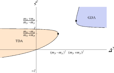
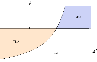
5.2.1 Soft-pion theorem for nucleon-to-pion GDAs

According to the partial conservation of the axial current (PCAC) hypothesis (see e.g. [140]) the following soft-pion theorem is valid for the matrix element of the three-quark light-cone operator $\widehat{O}_{\rho\tau\chi}^{\,\alpha\beta\gamma}$ (4.94) defining $\pi N$ GDAs:

$$\langle 0|\widehat{O}^{\alpha\beta\gamma}_{\rho\tau\chi}(1,\,2,\,3)|\pi_{a}N_{\iota}\rangle\Big{|}_{{\text{soft}\atop\text{pion}}}=-\frac{i}{f_{\pi}}\langle 0|\left[\widehat{Q}_{5}^{a},\,\widehat{O}^{\alpha\beta\gamma}_{\rho\tau\chi}(1,\,2,\,3)\right]|N_{\iota}\rangle\,.$$ (5.31)

The commutator of the chiral charge operator $\widehat{Q}^{5}_{a}$ with quark field operators is given by

$$\left[\widehat{Q}^{5}_{a},\ \Psi^{\alpha}_{\eta}\right]=-\frac{1}{2}(\sigma_{a})^{\alpha}_{\;\delta}\gamma^{5}_{\eta\tau}\Psi^{\delta}_{\tau}\,,$$ (5.32)

where $\sigma_{a}$ are the Pauli matrices. The commutator of the chiral charge operator $\widehat{Q}^{5}_{a}$ with the operator $\widehat{O}$ in (5.31) is computed with the help of the chain rule $[A,BCD]=[A,B]CD+B[A,C]D+BC[A,D]$. This allows to express $\pi N$ GDAs in terms of the leading twist nucleon DAs $M^{N\,\{12\}}$, $M^{N\,\{13\}}$ defined in (4.98):

$$4\langle 0|\widehat{O}^{\alpha\beta\gamma}_{\rho\tau\chi}(1,\,2,\,3)|\pi_{a}N_{\iota}\rangle\Big{|}_{{\text{soft}\atop\text{pion}}}=-\frac{i}{f_{\pi}}\langle 0|\left[\widehat{Q}_{5}^{a},\,\widehat{O}^{\alpha\beta\gamma}_{\rho\tau\chi}(1,\,2,\,3)\right]|N_{\iota}\rangle$$

$$=\frac{i}{2f_{\pi}}\Bigl{\{}(\sigma_{a})^{\alpha}_{\;\delta}\varepsilon^{\delta\beta}\delta^{\gamma}_{\iota}\gamma^{5}_{\rho\eta}M^{N\,\{13\}}_{\eta\tau\chi}(1,2,3)+(\sigma_{a})^{\alpha}_{\;\delta}\varepsilon^{\delta\gamma}\delta^{\beta}_{\iota}\gamma^{5}_{\rho\eta}M^{N\,\{12\}}_{\eta\tau\chi}(1,2,3)$$

$$+(\sigma_{a})^{\beta}_{\;\delta}\varepsilon^{\alpha\delta}\delta^{\gamma}_{\iota}\gamma^{5}_{\tau\eta}M^{N\,\{13\}}_{\rho\eta\chi}(1,2,3)+(\sigma_{a})^{\beta}_{\;\delta}\varepsilon^{\alpha\gamma}\delta^{\delta}_{\iota}\gamma^{5}_{\tau\eta}M^{N\,\{12\}}_{\rho\eta\chi}(1,2,3)$$

$$+(\sigma_{a})^{\gamma}_{\;\delta}\varepsilon^{\alpha\beta}\delta^{\delta}_{\iota}\gamma^{5}_{\chi\eta}M^{N\,\{13\}}_{\rho\tau\eta}(1,2,3)+(\sigma_{a})^{\gamma}_{\;\delta}\varepsilon^{\alpha\delta}\delta^{\beta}_{\iota}\gamma^{5}_{\chi\eta}M^{N\,\{12\}}_{\rho\tau\eta}(1,2,3)\Bigr{\}}\,.$$ (5.33)

The isospin parametrization for $\pi N$ GDAs is analogous to that of $\pi N$ TDAs described in Sec. 4.6. Employing the general isospin parametrization for the leading twist nucleon DAs (4.102) and the symmetry relations (4.104) together with the Fierz identities (LABEL:Fierz_nucleon_structures) we establish the consequences of the soft-pion theorem for the invariant isospin-$\frac{3}{2}$ and isospin-$\frac{1}{2}$ $\pi N$ GDAs. The invariant amplitudes $M^{(\pi N)_{3/2}}_{\rho\tau\chi}(1,\,2,\,3)$ and $M^{(\pi N)_{1/2}}_{\rho\tau\chi}(1,\,2,\,3)$ at the pion threshold are expressed in terms of the leading twist nucleon DA $\phi^{N}$ (4.109):

$$M^{(\pi N)_{3/2}}_{\rho\tau\chi}(1,\,2,\,3)\Big{|}_{{\text{soft}\atop\text{pion}}}=\frac{i}{2f_{\pi}}\Bigl{\{}\gamma^{5}_{\rho\eta}M^{N\,\{12\}}_{\eta\tau\chi}(1,\,2,\,3)-\gamma^{5}_{\chi\eta}M^{N\,\{12\}}_{\rho\tau\eta}(1,\,2,\,3)$$

$$+\gamma^{5}_{\rho\eta}M^{N\,\{13\}}_{\eta\tau\chi}(1,\,2,\,3)-\gamma^{5}_{\tau\eta}M^{N\,\{13\}}_{\rho\eta\chi}(1,\,2,\,3)\Bigr{\}}$$

$$=\frac{if_{N}}{f_{\pi}}\Bigl{\{}-\left(\gamma^{5}_{\chi\eta}v^{N}_{\rho\tau,\,\eta}\right)\frac{1}{2}\left[\phi^{N}(1,2,3)+\phi^{N}(2,1,3)+\phi^{N}(3,2,1)+\phi^{N}(3,1,2)\right]$$

$$-\left(\gamma^{5}_{\chi\eta}a^{N}_{\rho\tau,\,\eta}\right)\frac{1}{2}\left[-\phi^{N}(1,2,3)+\phi^{N}(2,1,3)-\phi^{N}(3,2,1)+\phi^{N}(3,1,2)\right]$$

$$-\left(\gamma^{5}_{\chi\eta}t^{N}_{\rho\tau,\,\eta}\right)\frac{1}{2}\left[\phi^{N}(1,3,2)+\phi^{N}(2,3,1)\right]\Bigr{\}}\,;$$ (5.34)

$$M^{(\pi N)_{1/2}\,\{12\}}_{\rho\tau\chi}(1,\,2,\,3)\Big{|}_{{\text{soft}\atop\text{pion}}}=\frac{i}{2f_{\pi}}\frac{1}{3}\Bigl{\{}\gamma^{5}_{\rho\eta}M^{N\,\{12\}}_{\eta\tau\chi}(1,\,2,\,3)+3\gamma^{5}_{\tau\eta}M^{N\,\{12\}}_{\rho\eta\chi}(1,\,2,\,3)$$

$$-\gamma^{5}_{\chi\eta}M^{N\,\{12\}}_{\rho\tau\eta}(1,\,2,\,3)-2\gamma^{5}_{\rho\eta}M^{N\,\{13\}}_{\eta\tau\chi}(1,\,2,\,3)+2\gamma^{5}_{\tau\eta}M^{N\,\{13\}}_{\rho\eta\chi}(1,\,2,\,3)\Bigr{\}}$$

$$=\frac{i}{f_{\pi}}\Bigl{\{}-\left(\gamma^{5}_{\chi\eta}v^{N}_{\rho\tau,\,\eta}\right)\frac{1}{12}\left[-\phi^{N}(1,2,3)-\phi^{N}(2,1,3)-4(\phi^{N}(3,1,2)+\phi^{N}(3,2,1))\right]$$

$$-\left(\gamma^{5}_{\chi\eta}a^{N}_{\rho\tau,\,\eta}\right)\frac{1}{12}\left[\phi^{N}(1,2,3)-\phi^{N}(2,1,3)-4(\phi^{N}(3,1,2)-\phi^{N}(3,2,1))\right]$$

$$-\left(\gamma^{5}_{\chi\eta}t^{N}_{\rho\tau,\,\eta}\right)\frac{5}{12}\left[\phi^{N}(1,3,2)+\phi^{N}(2,3,1)\right]\Bigr{\}}\,;$$ (5.35)

$$M^{(\pi N)_{1/2}\,\{13\}}_{\rho\tau\chi}(1,\,2,\,3)\Big{|}_{{\text{soft}\atop\text{pion}}}=M^{(\pi N)_{1/2}\,\{12\}}_{\rho\chi\tau}(1,\,3,\,2)\Big{|}_{{\text{soft}\atop\text{pion}}}.$$ (5.36)

$\pi N$ GDAs in the soft-pion limit (5.34), (5.35), (5.36) naturally satisfy the isospin-$\frac{3}{2}$ and isospin-$\frac{1}{2}$ symmetry and permutation symmetry relations (4.123), (4.121), (4.122) that provides an additional cross-check.

From (5.34), (5.35), (5.36), it is straightforward to verify that for particular $\pi N$ GDAs we recover the same soft-pion theorems that were established in Ref. [138].

• For $p\pi^{0}$ GDA we get

  $$4\langle 0|u_{\rho}(1)u_{\tau}(2)d_{\chi}(3)|p\pi^{0}\rangle\Big{|}_{{\text{soft}\atop\text{pion}}}=M^{(\pi N)_{1/2}\,\{12\}}_{\rho\tau\chi}(1,2,3)\Big{|}_{{\text{soft}\atop\text{pion}}}+\frac{2}{3}M^{(\pi N)_{3/2}}_{\rho\tau\chi}(1,2,3)\Big{|}_{{\text{soft}\atop\text{pion}}}$$

  $$=\frac{if_{N}}{f_{\pi}}\Bigl{\{}-\left(\gamma^{5}_{\chi\eta}v^{N}_{\rho\tau,\,\eta}\right)\frac{1}{4}\left(\phi^{N}(1,2,3)+\phi^{N}(2,1,3)\right)-\left(\gamma^{5}_{\chi\eta}a^{N}_{\rho\tau,\,\eta}\right)\frac{1}{4}\left(-\phi^{N}(1,2,3)+\phi^{N}(2,1,3)\right){}$$

  $$-\left(\gamma^{5}_{\chi\eta}t^{N}_{\rho\tau,\,\eta}\right)\frac{3}{4}\left(\phi^{N}(1,3,2)+\phi^{N}(2,3,1)\right)\Bigr{\}}\,;$$ (5.37)

• For $n\pi^{+}$ and $p\pi^{-}$ GDAs we get

  $$4\langle 0|u_{\rho}(1)u_{\tau}(2)d_{\chi}(3)|n\pi^{+}\rangle\Big{|}_{{\text{soft}\atop\text{pion}}}=-4\langle 0|d_{\rho}(1)d_{\tau}(2)u_{\chi}(3)|p\pi^{-}\rangle\Big{|}_{{\text{soft}\atop\text{pion}}}$$

  $$=\sqrt{2}M^{(\pi N)_{1/2}\,\{12\}}_{\rho\tau\chi}(1,2,3)\Big{|}_{{\text{soft}\atop\text{pion}}}-\frac{\sqrt{2}}{3}M^{(\pi N)_{3/2}}_{\rho\tau\chi}(1,2,3)\Big{|}_{{\text{soft}\atop\text{pion}}}$$

  $$=\frac{if_{N}}{f_{\pi}}\Bigm{\{}-\left(\gamma^{5}_{\chi\eta}v^{N}_{\rho\tau,\,\eta}\right)\frac{1}{2\sqrt{2}}\left[-\phi^{N}(1,2,3)-\phi^{N}(2,1,3)-2((\phi^{N}(3,1,2)+\phi^{N}(3,2,1))\right]$$

  $$-\left(\gamma^{5}_{\chi\eta}a^{N}_{\rho\tau,\,\eta}\right)\frac{1}{2\sqrt{2}}\left[\phi_{N}(1,2,3)-\phi^{N}(2,1,3)-2(\phi^{N}(3,1,2)-\phi^{N}(3,2,1))\right]$$

  $$-\left(\gamma^{5}_{\chi\eta}t^{N}_{\rho\tau,\,\eta}\right)\frac{1}{2\sqrt{2}}\left[\phi^{N}(1,3,2)+\phi^{N}(2,3,1)\right]\Bigm{\}}\,.$$ (5.38)

5.2.2 Soft-pion theorem for $\pi N$ TDAs in the chiral limit

To establish the consequences of the soft-pion theorem (5.31) for $\pi N$ TDAs we apply the crossing transformation to the matrix element (5.33). We assume smallness of possible non-analytic corrections and rely on the soft-pion theorem to work out the physical normalization of $\pi N$ TDAs. Below we quote the results in the chiral limit $m_{\pi}=0$.

The relation between the Dirac structures (4.55) of the $\pi N$ TDA parametrization (4.53) of Sec. 4.4 and those occurring in (5.34), (5.35) is given by:

$$\gamma^{5}_{\chi\eta}v^{N}_{\rho\tau,\,\eta}=\frac{1}{m_{N}}\left({v_{1}}_{\rho\tau,\,\chi}^{(\pi N)}-\frac{1}{2}{v_{2}}_{\rho\tau,\,\chi}^{(\pi N)}\right)\,;$$

$$\gamma^{5}_{\chi\eta}a^{N}_{\rho\tau,\,\eta}=\frac{1}{m_{N}}\left({a_{1}}_{\rho\tau,\,\chi}^{(\pi N)}-\frac{1}{2}{a_{2}}_{\rho\tau,\,\chi}^{(\pi N)}\right)\,;$$

$$\gamma^{5}_{\chi\eta}t^{N}_{\rho\tau,\,\eta}=-\frac{1}{m_{N}}\left({t_{1}}_{\rho\tau,\,\chi}^{(\pi N)}-\frac{1}{2}{t_{2}}_{\rho\tau,\,\chi}^{(\pi N)}\right)\,.$$ (5.39)

In the chiral limit $m_{\pi}=0$ this results in the following contributions to the independent isospin-$\frac{1}{2}$ and isospin-$\frac{3}{2}$ $\pi N$ TDAs (4.127), (4.130) regular at $\Delta^{2}=m_{N}^{2}$:

$$\phi^{(\pi N)_{1/2}}_{1}(x_{1},x_{2},x_{3},\xi=1,\Delta^{2}=m_{N}^{2})\Big{|}_{{{\rm soft}\atop{\rm pion}}}=\frac{1}{24}\phi^{N}\left(\frac{x_{1}}{2},\frac{x_{2}}{2},\frac{x_{3}}{2}\right)+\frac{1}{6}\phi^{N}\left(\frac{x_{3}}{2},\frac{x_{2}}{2},\frac{x_{1}}{2}\right)\,;$$

$$\phi^{(\pi N)_{1/2}}_{2}(x_{1},x_{2},x_{3},\xi=1,\Delta^{2}=m_{N}^{2})\Big{|}_{{{\rm soft}\atop{\rm pion}}}=-\frac{1}{2}\phi^{(\pi N)_{1/2}}_{1}(x_{1},x_{2},x_{3},\xi=1,\Delta^{2}=m_{N}^{2})\Big{|}_{{{\rm soft}\atop{\rm pion}}}\,;$$

$$\phi^{(\pi N)_{3/2}}_{1}(x_{1},x_{2},x_{3},\xi=1,\Delta^{2}=m_{N}^{2})\Big{|}_{{{\rm soft}\atop{\rm pion}}}=\frac{1}{4}\left(\phi^{N}\left(\frac{x_{1}}{2},\frac{x_{2}}{2},\frac{x_{3}}{2}\right)+\phi^{N}\left(\frac{x_{3}}{2},\frac{x_{2}}{2},\frac{x_{1}}{2}\right)\right)\,;$$

$$\phi^{(\pi N)_{3/2}}_{2}(x_{1},x_{2},x_{3},\xi=1,\Delta^{2}=m_{N}^{2})\Big{|}_{{{\rm soft}\atop{\rm pion}}}=-\frac{1}{2}\phi^{(\pi N)_{3/2}}_{1}(x_{1},x_{2},x_{3},\xi=1,\Delta^{2}=m_{N}^{2})\Big{|}_{{{\rm soft}\atop{\rm pion}}}\,.$$ (5.40)

Now employing the isospin parametrization and the definitions (4.129), (4.132) we determine the physical normalization of $\pi N$ TDAs from the soft-pion theorem for all possible isospin channels within the parametrization (4.53) of Sec. 4.4.

• For $p\to\pi^{0}$ $uud$ TDAs we get

  $$V_{1}^{\pi^{0}p}(x_{1},\,x_{2},\,x_{3},\xi=1,\Delta^{2}=m_{N}^{2})=-\frac{1}{16}\left(\phi^{N}\left(\frac{x_{1}}{2},\frac{x_{2}}{2},\frac{x_{3}}{2}\right)+\phi^{N}\left(\frac{x_{2}}{2},\frac{x_{1}}{2},\frac{x_{3}}{2}\right)\right);{}$$

  $$V_{2}^{\pi^{0}p}(x_{1},\,x_{2},\,x_{3},\xi=1,\Delta^{2}=m_{N}^{2})=-\frac{1}{2}V_{1}^{\pi^{0}p}(x_{1},\,x_{2},\,x_{3},\xi=1,\Delta^{2}=m_{N}^{2});{}$$

  $$A_{1}^{\pi^{0}p}(x_{1},\,x_{2},\,x_{3},\xi=1,\Delta^{2}=m_{N}^{2})=-\frac{1}{16}\left(-\phi^{N}\left(\frac{x_{1}}{2},\frac{x_{2}}{2},\frac{x_{3}}{2}\right)+\phi^{N}\left(\frac{x_{2}}{2},\frac{x_{1}}{2},\frac{x_{3}}{2}\right)\right);{}$$

  $$A_{2}^{\pi^{0}p}(x_{1},\,x_{2},\,x_{3},\xi=1,\Delta^{2}=m_{N}^{2})=-\frac{1}{2}A_{1}^{\pi^{0}p}(x_{1},\,x_{2},\,x_{3},\xi=1,\Delta^{2}=m_{N}^{2});{}$$

  $$T_{1}^{\pi^{0}p}(x_{1},\,x_{2},\,x_{3},\xi=1,\Delta^{2}=m_{N}^{2})=\frac{3}{16}\left(\phi^{N}\left(\frac{x_{1}}{2},\frac{x_{3}}{2},\frac{x_{2}}{2}\right)+\phi^{N}\left(\frac{x_{2}}{2},\frac{x_{3}}{2},\frac{x_{1}}{2}\right)\right);{}$$

  $$T_{2}^{\pi^{0}p}(x_{1},\,x_{2},\,x_{3},\xi=1,\Delta^{2}=m_{N}^{2})=-\frac{1}{2}T_{1}^{\pi^{0}p}(x_{1},\,x_{2},\,x_{3},\xi=1,\Delta^{2}=m_{N}^{2});{}$$

  $$T_{3}^{\pi^{0}p}(x_{1},\,x_{2},\,x_{3},\xi=1,\Delta^{2}=m_{N}^{2})=T_{4}^{\pi^{0}p}(x_{1},\,x_{2},\,x_{3},\xi=1,\Delta^{2}=m_{N}^{2})=0\,.$$ (5.41)

• For $n\to\pi^{-}$ $uud$ and $p\to\pi^{+}$ $ddu$ TDAs we get

  $$V_{1}^{\pi^{-}n}(x_{1},\,x_{2},\,x_{3},\xi=1,\Delta^{2}=m_{N}^{2})=-V_{1}^{\pi^{+}p}(x_{1},\,x_{2},\,x_{3},\xi=1,\Delta^{2}=m_{N}^{2}){}$$

  $$=\frac{1}{8\sqrt{2}}\left(\phi^{N}\left(\frac{x_{1}}{2},\frac{x_{2}}{2},\frac{x_{3}}{2}\right)+\phi^{N}\left(\frac{x_{2}}{2},\frac{x_{1}}{2},\frac{x_{3}}{2}\right)+2\phi^{N}\left(\frac{x_{3}}{2},\frac{x_{1}}{2},\frac{x_{2}}{2}\right)+2\phi^{N}\left(\frac{x_{3}}{2},\frac{x_{2}}{2},\frac{x_{1}}{2}\right)\right);{}$$

  $$V_{2}^{\{\pi^{+}p,\,\pi^{-}n\}}(x_{1},\,x_{2},\,x_{3},\xi=1,\Delta^{2}=m_{N}^{2})=-\frac{1}{2}V_{1}^{\{\pi^{+}p,\,\pi^{-}n\}}(x_{1},\,x_{2},\,x_{3},\xi=1,\Delta^{2}=m_{N}^{2});{}$$

  $$A_{1}^{\pi^{-}n}(x_{1},\,x_{2},\,x_{3},\xi=1,\Delta^{2}=m_{N}^{2})=-A_{1}^{\pi^{+}p}(x_{1},\,x_{2},\,x_{3},\xi=1,\Delta^{2}=m_{N}^{2}){}$$

  $$=\frac{1}{8\sqrt{2}}\left(-\phi^{N}\left(\frac{x_{1}}{2},\frac{x_{2}}{2},\frac{x_{3}}{2}\right)+\phi^{N}\left(\frac{x_{2}}{2},\frac{x_{1}}{2},\frac{x_{3}}{2}\right)-2\phi^{N}\left(\frac{x_{3}}{2},\frac{x_{1}}{2},\frac{x_{2}}{2}\right)+2\phi^{N}\left(\frac{x_{3}}{2},\frac{x_{2}}{2},\frac{x_{1}}{2}\right)\right);{}$$

  $$A_{2}^{\{\pi^{+}p,\,\pi^{-}n\}}(x_{1},\,x_{2},\,x_{3},\xi=1,\Delta^{2}=m_{N}^{2})=-\frac{1}{2}A_{1}^{\{\pi^{+}p,\,\pi^{-}n\}}(x_{1},\,x_{2},\,x_{3},\xi=1,\Delta^{2}=m_{N}^{2});{}$$

  $$T_{1}^{\pi^{-}n}(x_{1},\,x_{2},\,x_{3},\xi=1,\Delta^{2}=m_{N}^{2})=-T_{1}^{\pi^{+}p}(x_{1},\,x_{2},\,x_{3},\xi=1,\Delta^{2}=m_{N}^{2}){}$$

  $$=\frac{1}{8\sqrt{2}}\left(\phi^{N}\left(\frac{x_{1}}{2},\frac{x_{3}}{2},\frac{x_{2}}{2}\right)+\phi^{N}\left(\frac{x_{2}}{2},\frac{x_{3}}{2},\frac{x_{1}}{2}\right)\right);{}$$

  $$T_{2}^{\{\pi^{+}p,\,\pi^{-}n\}}(x_{1},\,x_{2},\,x_{3},\xi=1,\Delta^{2}=m_{N}^{2})=-\frac{1}{2}T_{1}^{\{\pi^{+}p,\,\pi^{-}n\}}(x_{1},\,x_{2},\,x_{3},\xi=1,\Delta^{2}=m_{N}^{2});{}$$

  $$T_{3,4}^{\{\pi^{+}p,\,\pi^{-}n\}}(x_{1},\,x_{2},\,x_{3},\xi=1,\Delta^{2}=m_{N}^{2})=0.$$ (5.42)

The soft-pion theorem (5.41) was employed in Ref. [37] to construct a simple phenomenological model for $\pi N$ TDAs:

$$\left\{V_{1}^{p\pi^{0}},A_{1}^{p\pi^{0}}\right\}\left(x_{i},\xi\right)=-\frac{1}{2}\cdot\frac{1}{4\xi}\left\{V^{p},A^{p}\right\}\left(\frac{x_{i}}{2\xi}\right);\quad T_{1}^{p\pi^{0}}\left(x_{i},\xi\right)=\frac{1}{2}\cdot\frac{3}{4\xi}T^{p}\left(\frac{x_{i}}{2\xi}\right);{}$$

$$V_{1}^{p\pi^{+}}\left(x_{i},\xi\right)=-\frac{\sqrt{2}}{2}\cdot\frac{1}{4\xi}\left(V^{p}\left(\frac{x_{1}}{2\xi},\frac{x_{2}}{2\xi},\frac{x_{3}}{2\xi}\right)+V^{p}\left(\frac{x_{3}}{2\xi},\frac{x_{1}}{2\xi},\frac{x_{2}}{2\xi}\right)+V^{p}\left(\frac{x_{2}}{2\xi},\frac{x_{3}}{2\xi},\frac{x_{1}}{2\xi}\right){}\right.$$

$$\left.-A^{p}\left(\frac{x_{3}}{2\xi},\frac{x_{1}}{2\xi},\frac{x_{2}}{2\xi}\right)-A^{p}\left(\frac{x_{3}}{2\xi},\frac{x_{2}}{2\xi},\frac{x_{1}}{2\xi}\right)\right);{}$$

$$A_{1}^{p\pi^{+}}\left(x_{i},\xi\right)=-\frac{\sqrt{2}}{2}\cdot\frac{1}{4\xi}\left(A^{p}\left(\frac{x_{1}}{2\xi},\frac{x_{2}}{2\xi},\frac{x_{3}}{2\xi}\right)-A^{p}\left(\frac{x_{3}}{2\xi},\frac{x_{1}}{2\xi},\frac{x_{2}}{2\xi}\right)-A^{p}\left(\frac{x_{2}}{2\xi},\frac{x_{3}}{2\xi},\frac{x_{1}}{2\xi}\right)\right.{}$$

$$\left.+V^{p}\left(\frac{x_{3}}{2\xi},\frac{x_{1}}{2\xi},\frac{x_{2}}{2\xi}\right)-V^{p}\left(\frac{x_{3}}{2\xi},\frac{x_{2}}{2\xi},\frac{x_{1}}{2\xi}\right)\right);{}$$

$$T_{1}^{p\pi^{+}}\left(x_{i},\xi\right)=-\frac{\sqrt{2}}{2}\cdot\frac{1}{4\xi}T^{p}\left(\frac{x_{i}}{2\xi}\right),$$ (5.43)

where $V^{p}(y_{1},y_{2},y_{3})$, $A^{p}(y_{1},y_{2},y_{3})$ and $T^{p}(y_{1},y_{2},y_{3})$ stand for the usual leading twist-$3$ nucleon DAs [146].

Despite its obvious drawbacks (like the very narrow validity range limited to the close vicinity of the threshold and lack of an intrinsic $\Delta^{2}$-dependence) the model (5.43) for the first time provided a quantitative estimate of the physical normalization for $\pi N$ TDAs. In particular, the predictions of the model (5.43) were employed in the first feasibility study [35] for accessing $\pi N$ TDAs with P̄ANDA through $\bar{p}p\to\gamma^{*}\pi^{0}$.

5.2.3 A model for quadruple distributions with input from chiral dynamics

A common strategy for modeling GPDs is to rely on extrapolation of forward partonic densities with the help of an Ansatz for the corresponding double distributions. The latter are usually parameterized as forward partonic densities times profile functions, which generate the skewness dependence. The so-called Radyushkin’s double distribution Ansatz [73] saw an extensive application in the GPD phenomenology.

In this subsection, using the results of Sec. 4.5.2, we consider a possible generalization [21] of this technique for the case of $\pi N$ TDAs. The key difference here is that nucleon-to-meson TDAs lack a comprehensible forward limit $\xi=0$; however, due to the soft-pion theorem presented in Sec. 5.2.1, $\pi N$ TDAs are constrained in a complementary $\xi=1$ limit and reduce to particular combinations of nucleon DAs.

To rewrite the spectral representation (4.84) for $\pi N$ TDAs in a suitable form we switch to the following combinations of the spectral parameters:

$$\kappa_{i}=\alpha_{i}+\beta_{i}\,;\ \ \ \theta_{i}=\frac{1}{2}\sum_{k,l=1}^{3}\varepsilon_{ikl}(\alpha_{k}+\beta_{k});$$

$$\mu_{i}=\alpha_{i}-\beta_{i}\,;\ \ \ \lambda_{i}=\frac{1}{2}\sum_{k,l=1}^{3}\varepsilon_{ikl}(\alpha_{k}-\beta_{k}).$$ (5.44)

The index $i=1,\,2,\,3$ here refers to a coordinated choice of the quark–diquark coordinates (4.45). After the change of integration variables the spectral representation (4.84) reads:

$$H(w_{i},\,v_{i},\,\xi)=\int_{-1}^{1}d\kappa_{i}\int_{-\frac{1-\kappa_{i}}{2}}^{\frac{1-\kappa_{i}}{2}}d\theta_{i}\int_{-1}^{1}d\mu_{i}\int_{-\frac{1-\mu_{i}}{2}}^{\frac{1-\mu_{i}}{2}}d\lambda_{i}\,\delta\left(w_{i}-\frac{\kappa_{i}-\mu_{i}}{2}(1-\xi)-\kappa_{i}\xi\right)$$

$$\times\delta\left(v_{i}-\frac{\theta_{i}-\lambda_{i}}{2}(1-\xi)-\theta_{i}\xi\right)\,\frac{1}{4}F_{i}(\kappa_{i},\,\theta_{i},\,\mu_{i},\,\lambda_{i}).$$ (5.45)

Below we summarize the explicit expressions for $\pi N$ TDAs from the spectral representation (5.45) in the ERBL-like and DGLAP-like domains (see Sec. 4.3). We employ the following shortened notation for the spectral density:

$$F_{i}(....)\equiv F_{i}\left(\kappa_{i},\,\theta_{i},\,\frac{\kappa_{i}(1+\xi)-2w_{i}}{1-\xi},\,\frac{\theta_{i}(1+\xi)-2v_{i}}{1-\xi}\right),$$ (5.46)

where $F$ is the quadruple distribution (4.85).

• DGLAP-like type I domain $w_{i}\in[-1;\,-\xi]$; $v_{i}\in[\xi^{\prime}_{i};\,1-\xi^{\prime}_{i}+\xi]$:

  $$H(w_{i},v_{i},\xi)=\frac{1}{(1-\xi)^{2}}\int_{-1}^{\frac{1-2v_{i}+w_{i}}{1+\xi}}d\kappa_{i}\int_{\frac{\kappa_{i}}{2}-\frac{1}{1+\xi}(w_{i}-2v_{i}+\frac{1-\xi}{2})}^{\frac{1-\kappa_{i}}{2}}d\theta_{i}F_{i}(....);$$ (5.47)

• DGLAP-like type II domain $w_{i}\in[-1;\,-\xi]$; $v\in[-\xi^{\prime}_{i};\,\xi^{\prime}_{i}]$:

  $$H(w_{i},v_{i},\xi)=\frac{1}{(1-\xi)^{2}}\int_{-1}^{\frac{1-\xi+2w_{i}}{1+\xi}}d\kappa_{i}\int_{\frac{\kappa_{i}}{2}-\frac{1}{1+\xi}(w_{i}-2v_{i}+\frac{1-\xi}{2})}^{-\frac{\kappa_{i}}{2}+\frac{1}{1+\xi}(w+2v+\frac{1-\xi}{2})}d\theta_{i}F_{i}(....);$$ (5.48)

• DGLAP-like type I domain $w_{i}\in[-1;\,-\xi]$; $v_{i}\in[-1+\xi^{\prime}_{i}-\xi;\,-\xi^{\prime}_{i}]$:

  $$H(w_{i},v_{i},\xi)=\frac{1}{(1-\xi)^{2}}\int_{-1}^{\frac{1+2v_{i}+w_{i}}{1+\xi}}d\kappa_{i}\int_{-\frac{1-\kappa_{i}}{2}}^{-\frac{\kappa_{i}}{2}+\frac{1}{1+\xi}(w_{i}+2v_{i}+\frac{1-\xi}{2})}d\theta_{i}F_{i}(....);$$ (5.49)

• DGLAP-like type II domain $w_{i}\in[-\xi;\,1]$; $v_{i}\in[|\xi^{\prime}_{i}|;\,1-\xi+\xi^{\prime}_{i}]$:

  $$H(w_{i},v_{i},\xi)=\frac{1}{(1-\xi)^{2}}\int_{\frac{-1+\xi+2w_{i}}{1+\xi}}^{\frac{1-2v_{i}+w_{i}}{1+\xi}}d\kappa_{i}\int_{\frac{\kappa_{i}}{2}-\frac{1}{1+\xi}(w_{i}-2v_{i}+\frac{1-\xi}{2})}^{\frac{1-\kappa_{i}}{2}}d\theta_{i}F_{i}(....);$$ (5.50)

• ERBL-like domain $w_{i}\in[-\xi;\,\xi]$; $v_{i}\in[-\xi^{\prime}_{i};\,+\xi^{\prime}_{i}]$:

  $$H(w_{i},v_{i},\xi)=\frac{1}{(1-\xi)^{2}}\int_{\frac{-1+\xi+2w_{i}}{1+\xi}}^{\frac{1-\xi+2w_{i}}{1+\xi}}d\kappa_{i}\int_{\frac{\kappa_{i}}{2}-\frac{1}{1+\xi}(w_{i}-2v_{i}+\frac{1-\xi}{2})}^{-\frac{\kappa_{i}}{2}+\frac{1}{1+\xi}(w_{i}+2v_{i}+\frac{1-\xi}{2})}d\theta_{i}F_{i}(....);$$ (5.51)

• DGLAP-like type II domain $w_{i}\in[-\xi;\,1]$; $v_{i}\in[-1+\xi-\xi^{\prime}_{i};\,-|\xi^{\prime}_{i}|]$:

  $$H(w_{i},v_{i},\xi)=\frac{1}{(1-\xi)^{2}}\int_{\frac{-1+\xi+2w_{i}}{1+\xi}}^{\frac{1+2v_{i}+w_{i}}{1+\xi}}d\kappa_{i}\int_{-\frac{1-\kappa_{i}}{2}}^{-\frac{\kappa_{i}}{2}+\frac{1}{1+\xi}(w_{i}+2v_{i}+\frac{1-\xi}{2})}d\theta_{i}F_{i}(....);$$ (5.52)

• DGLAP-like type II domain $w_{i}\in[\xi;\,1]$; $v_{i}\in[\xi^{\prime}_{i};\,-\xi^{\prime}_{i}]$:

  $$H(w_{i},v_{i},\xi)=\frac{1}{(1-\xi)^{2}}\int_{\frac{-1+\xi+2w_{i}}{1+\xi}}^{1}d\kappa_{i}\int_{-\frac{1-\kappa_{i}}{2}}^{\frac{1-\kappa_{i}}{2}}d\theta_{i}F_{i}(....);$$ (5.53)

• For $w_{i}$ and $v_{i}$ outside the domain $w_{i}\in[-1;\,1]$ and $v_{i}\in[-1+|\xi_{i}-\xi^{\prime}_{i}|;\,1-|\xi_{i}-\xi^{\prime}_{i}|]$ the spectral representation (5.45) provides a vanishing result for $0\leq\xi\leq 1$.

The suggested factorized Ansatz for quadruple distributions $F_{i}$ has the form

$$F_{i}(\kappa_{i},\,\theta_{i},\,\mu_{i},\,\lambda_{i})=4\Phi(\kappa_{i},\,\theta_{i})\,h(\mu_{i},\,\lambda_{i}),$$ (5.54)

with the profile function $h(\mu_{i},\,\lambda_{i})$ normalized as

$$\int_{-1}^{1}d\mu_{i}\int_{-\frac{1-\mu_{i}}{2}}^{\frac{1-\mu_{i}}{2}}d\lambda_{i}\,h(\mu_{i},\,\lambda_{i})=1.$$ (5.55)

With help of the spectral representation (5.45), one can check that in the limit $\xi\rightarrow 1$ $H_{i}$ indeed reduces to

$$H(w_{i},\,v_{i},\,\xi=1)=\Phi(w_{i},\,v_{i}).$$ (5.56)

As the phenomenological input for $\Phi(w_{i},\,v_{i})$ it is natural to use the combinations of nucleon DAs (5.41), (5.42) to which $\pi N$ TDAs reduce in the limit $\xi\to 1$ due to the soft-pion theorem.

We denote the corresponding combinations of nucleon DAs as $\Phi(y_{1},y_{2},y_{3})$. These are functions of three momentum fractions $y_{i}$ ($0\leq y_{i}\leq 1$) satisfying the condition $\sum_{i}y_{i}=1$. According to the particular choice of quark–diquark coordinates in (4.80), one has to employ in (5.54):

$$\Phi(\kappa_{1},\theta_{1})\equiv\frac{1}{4}\Phi\left(\frac{\kappa_{1}+1}{2},\,\frac{1-\kappa_{1}+2\theta_{1}}{4},\,\frac{1-\kappa_{1}-2\theta_{1}}{4}\right);$$

$$\Phi(\kappa_{2},\theta_{2})\equiv\frac{1}{4}\Phi\left(\frac{1-\kappa_{2}-2\theta_{2}}{4},\,\frac{\kappa_{2}+1}{2},\,\frac{1-\kappa_{2}+2\theta_{2}}{4}\right);$$

$$\Phi(\kappa_{3},\theta_{3})\equiv\frac{1}{4}\Phi\left(\frac{1-\kappa_{3}+2\theta_{3}}{4},\,\frac{1-\kappa_{3}-2\theta_{3}}{4},\,\frac{\kappa_{3}+1}{2}\right).$$ (5.57)

The profile function $h(\mu_{i},\,\lambda_{i})$ also has the support of a baryon DA: $-1\leq\mu_{i}\leq 1$; $-\frac{1-\mu_{i}}{2}\leq\lambda_{i}\leq\frac{1-\mu_{i}}{2}$. Contrary to the GPD case, no symmetry constraint from hermiticity and time-reversal invariance occurs for quadruple distributions. Therefore, we are free to employ an arbitrary shape for the profile function $h(\mu_{i},\,\lambda_{i})$. The simplest possible choice is to assume that it is determined by the asymptotic form of a baryon DA ($120y_{1}y_{2}y_{3}$ with $\sum_{i}y_{i}=1$):

$$h(\mu_{i},\,\lambda_{i})=\frac{15}{16}\,(1+\mu_{i})((1-\mu_{i})^{2}-4\lambda_{i}^{2})\,.$$ (5.58)

The normalization (5.55) is obviously maintained and the profile function vanishes at the borders of its domain of definition.

For the $\Delta^{2}$-dependence the most straightforward solution is the factorized form of $\Delta^{2}$ dependence for quadruple distributions (5.54):

$$F_{i}(\kappa_{i},\,\theta_{i},\,\mu_{i},\,\lambda_{i},\Delta^{2})=4\Phi(\kappa_{i},\,\theta_{i})\,h(\mu_{i},\,\lambda_{i})\times G(\Delta^{2}),$$ (5.59)

where $G(\Delta^{2})$ is the $\pi N$ transition form factor of the local three quark operator $\widehat{O}^{\alpha\beta\gamma}_{\rho\tau\chi}(0,0,0)$ (4.94) for which e.g. a dipole formula $G(\Delta^{2})\sim(M_{D}^{2}-\Delta^{2})^{-2}$ can be adopted. Let us however note that a factorized form of the $\Delta^{2}$-dependence is known to be oversimplified and was much criticized in the GPD case (see e.g. discussion in [144]).

Let us briefly summarize the key features of the phenomenological model for $\pi N$ TDAs based on the factorized Ansatz (5.45).

• The model can be employed for $\pi N$ TDAs (4.53) corresponding to the fully covariant set of the Dirac structures (4.56). These TDAs satisfy the polynomiality property in its simple form (see discussion in Sec. 4.4).

• By construction, the threshold soft-pion limit of $\pi N$ TDAs required by the soft-pion theorem (5.33) is assured.

• As phenomenological input one can employ various phenomenological solutions for leading twist nucleon DAs, for a review see [26, 27].

• The model provides lively $x_{i}$ and $\xi$ dependencies for $\pi N$ TDAs.

• The support properties of $\pi N$ TDAs are satisfied.

• The polynomiality property (4.65) of $x_{i}$ Mellin moments of $\pi N$ TDAs is generally ensured. However, to satisfy this property in its complete form a $D$-term like contribution with a pure ERBL-like support is to be added to $\pi N$ TDAs resulting from the spectral representation.

In conclusion, we present the phenomenological “two component” model for $\pi N$ TDAs. The model includes a spectral part contribution built with the factorized Ansatz (5.59) for quadruple distributions with the input from the soft-pion theorem and the cross-channel nucleon exchange contribution of Sec. 5.1.1.

We quote the result within the $\pi N$ parametrization of Sec. 4.1.1 corresponding to the set of the Dirac structures (4.6). This parametrization turns to be better suited for the phenomenological applications as it allows a clear separation of contributions proportional to $\Delta_{T}^{2}$ that are presumably small in the near-backward kinematics. Note that within this parametrization the spectral part contribution with input from the soft-pion theorem occurs only for $\pi N$ TDAs $V_{1}^{\pi N}$, $A_{1}^{\pi N}$ and $T_{1}^{\pi N}$.

• For the $uud$ proton-to-$\pi^{0}$ TDAs the suggested model reads:

  $$V_{1}^{\pi^{0}p}(x_{1},\,x_{2},\,x_{3},\xi)\Big{|}_{\text{set of Eq.\leavevmode\nobreak\ (\ref{Def_DirStr_piN_DeltaT})}}{}$$

  $$=\Bigl{\{}\text{Spectral part with}\;\Phi\;\text{from Eq.\leavevmode\nobreak\ (\ref{SoftPion_p_pi0})}\Bigr{\}}+\frac{1-\xi}{1+\xi}\left\{V_{1}^{(\pi N)_{1/2}}(x_{1},\,x_{2},\,x_{3},\xi)\Big{|}_{N(940)},\;\text{ Eq.\leavevmode\nobreak\ (\ref{Nucleon_exchange_contr_VAT})}\right\};{}$$

  $$A_{1}^{\pi^{0}p}(x_{1},\,x_{2},\,x_{3},\xi)\Big{|}_{\text{set of Eq.\leavevmode\nobreak\ (\ref{Def_DirStr_piN_DeltaT})}}{}$$

  $$=\Bigl{\{}\text{Spectral part with}\;\Phi\;\text{from Eq.\leavevmode\nobreak\ (\ref{SoftPion_p_pi0})}\Bigr{\}}+\frac{1-\xi}{1+\xi}\left\{A_{1}^{(\pi N)_{1/2}}(x_{1},\,x_{2},\,x_{3},\xi)\Big{|}_{N(940)},\;\text{ Eq.\leavevmode\nobreak\ (\ref{Nucleon_exchange_contr_VAT})}\right\};{}$$

  $$T_{1}^{\pi^{0}p}(x_{1},\,x_{2},\,x_{3},\xi)\Big{|}_{\text{set of Eq.\leavevmode\nobreak\ (\ref{Def_DirStr_piN_DeltaT})}}{}$$

  $$=\Bigl{\{}\text{Spectral part with}\;\Phi\;\text{from Eq.\leavevmode\nobreak\ (\ref{SoftPion_p_pi0})}\Bigr{\}}+\frac{1-\xi}{1+\xi}\left\{T_{1}^{(\pi N)_{1/2}}(x_{1},\,x_{2},\,x_{3},\xi)\Big{|}_{N(940)},\;\text{ Eq.\leavevmode\nobreak\ (\ref{Nucleon_exchange_contr_VAT})}\right\};{}$$

  $$\{V_{2},\,A_{2},\,T_{2}\}^{\pi^{0}p}(x_{1},\,x_{2},\,x_{3},\xi)\Big{|}_{\text{set of Eq.\leavevmode\nobreak\ (\ref{Def_DirStr_piN_DeltaT})}}{}$$

  $$=\left\{\{V_{1},\,A_{1},\,T_{1}\}^{(\pi N)_{1/2}}(x_{1},\,x_{2},\,x_{3},\xi)\Big{|}_{N(940)},\;\text{Eq.\leavevmode\nobreak\ (\ref{Nucleon_exchange_contr_VAT})}\right\}{}$$

  $$\{T_{3},\,T_{4}\}^{\pi^{0}p}(x_{1},\,x_{2},\,x_{3},\xi)\Big{|}_{\text{set of Eq.\leavevmode\nobreak\ (\ref{Def_DirStr_piN_DeltaT})}}=0.$$ (5.60)

• For the $ddu$ proton-to-$\pi^{+}$ and $uud$ neutron-to-$\pi^{-}$ TDAs the suggested model reads:

  $$V_{1}^{\pi^{+}p}(x_{1},\,x_{2},\,x_{3},\xi)\Big{|}_{\text{set of Eq.\leavevmode\nobreak\ (\ref{Def_DirStr_piN_DeltaT})}}=-V_{1}^{\pi^{-}n}(x_{1},\,x_{2},\,x_{3},\xi)\Big{|}_{\text{set of Eq.\leavevmode\nobreak\ (\ref{Def_DirStr_piN_DeltaT})}}{}$$

  $$=\Bigl{\{}\text{Spectral part with}\;\Phi\;\text{from Eq.\leavevmode\nobreak\ (\ref{SoftPion_p_pi+})}\Bigr{\}}-\sqrt{2}\frac{1-\xi}{1+\xi}\left\{V_{1}^{(\pi N)_{1/2}}(x_{1},\,x_{2},\,x_{3},\xi)\Big{|}_{N(940)},\;\text{Eq.\leavevmode\nobreak\ (\ref{Nucleon_exchange_contr_VAT})}\right\};{}$$

  $$A_{1}^{\pi^{+}p}(x_{1},\,x_{2},\,x_{3},\xi)\Big{|}_{\text{set of Eq.\leavevmode\nobreak\ (\ref{Def_DirStr_piN_DeltaT})}}=-A_{1}^{\pi^{-}n}(x_{1},\,x_{2},\,x_{3},\xi)\Big{|}_{\text{set of Eq.\leavevmode\nobreak\ (\ref{Def_DirStr_piN_DeltaT})}}{}$$

  $$=\Bigl{\{}\text{Spectral part with}\;\Phi\;\text{from Eq.\leavevmode\nobreak\ (\ref{SoftPion_p_pi+})}\Bigr{\}}-\sqrt{2}\frac{1-\xi}{1+\xi}\left\{A_{1}^{(\pi N)_{1/2}}(x_{1},\,x_{2},\,x_{3},\xi)\Big{|}_{N(940)},\;\text{Eq.\leavevmode\nobreak\ (\ref{Nucleon_exchange_contr_VAT})}\right\};{}$$

  $$T_{1}^{\pi^{+}p}(x_{1},\,x_{2},\,x_{3},\xi)\Big{|}_{\text{set of Eq.\leavevmode\nobreak\ (\ref{Def_DirStr_piN_DeltaT})}}=-T_{1}^{\pi^{-}n}(x_{1},\,x_{2},\,x_{3},\xi)\Big{|}_{\text{set of Eq.\leavevmode\nobreak\ (\ref{Def_DirStr_piN_DeltaT})}}{}$$

  $$=\Bigl{\{}\text{Spectral part with}\;\Phi\;\text{from eq.\leavevmode\nobreak\ (\ref{SoftPion_p_pi+})}\Bigr{\}}-\sqrt{2}\frac{1-\xi}{1+\xi}\left\{T_{1}^{(\pi N)_{1/2}}(x_{1},\,x_{2},\,x_{3},\xi)\Big{|}_{N(940)},\;\text{Eq.\leavevmode\nobreak\ (\ref{Nucleon_exchange_contr_VAT})}\right\};{}$$

  $$\{V_{2},\,A_{2},\,T_{2}\}^{\pi^{+}p}(x_{1},\,x_{2},\,x_{3},\xi)\Big{|}_{\text{set of Eq.\leavevmode\nobreak\ (\ref{Def_DirStr_piN_DeltaT})}}=-\{V_{2},\,A_{2},\,T_{2}\}^{\pi^{-}n}(x_{1},\,x_{2},\,x_{3},\xi)\Big{|}_{\text{set of Eq.\leavevmode\nobreak\ (\ref{Def_DirStr_piN_DeltaT})}}{}$$

  $$=-\sqrt{2}\left\{\{V_{1},\,A_{1},\,T_{1}\}^{(\pi N)_{1/2}}(x_{1},\,x_{2},\,x_{3},\xi)\Big{|}_{N(940)},\,\text{Eq.\leavevmode\nobreak\ (\ref{Nucleon_exchange_contr_VAT}) }\right\};{}$$

  $$\{T_{3},\,T_{4}\}^{\pi^{+}p}(x_{1},\,x_{2},\,x_{3},\xi)\Big{|}_{\text{set of Eq.\leavevmode\nobreak\ (\ref{Def_DirStr_piN_DeltaT})}}=-\{T_{3},\,T_{4}\}^{\pi^{-}n}(x_{1},\,x_{2},\,x_{3},\xi)\Big{|}_{\text{set of Eq.\leavevmode\nobreak\ (\ref{Def_DirStr_piN_DeltaT})}}=0.$$ (5.61)

Eqs. (5.60), (5.61) clearly show that we avoid the double counting problem between the spectral part and the cross-channel nucleon exchange parts for $\pi N$ TDAs $\{V_{1},\,A_{1},\,T_{1}\}^{\pi N}$ since the nucleon exchange parts turn into zero for $\xi=1$; and therefore, do not affect the normalization in the soft-pion limit $\xi=1$, $\Delta^{2}=m_{N}^{2}$.

In Fig. 23 we show the spectral part of $\pi^{0}p$ TDAs $V_{1}^{\pi^{0}p}$, $A_{1}^{\pi^{0}p}$ and $T_{1}^{\pi^{0}p}$ (5.60) computed in the model based on the factorized Ansatz (5.54) with the profile function (5.58) as functions of quark–diquark coordinates $w\equiv w_{3}$, $v\equiv v_{3}$ for $\xi=\frac{1}{2}$. We also present the combinations of nucleon DAs (5.41), to which the corresponding TDAs are reduced in the limit $\xi=1$. Chernyak–Ogloblin–Zhitnitsky (COZ) phenomenological solution for nucleon DAs [25] is used as numerical input.

Figure 23: Spectral part of $\pi^{0}p$ TDAs $V_{1}^{\pi^{0}p}$, $A_{1}^{\pi^{0}p}$ and $T_{1}^{\pi^{0}p}$ (5.60) computed in the model based on the factorized Ansatz (5.54) with the profile function (5.58) as functions of quark–diquark coordinates $w\equiv w_{3}$, $v\equiv v_{3}$. Upper row shows the combination of nucleon DAs (5.41) to which the corresponding TDAs are reduced in the limit $\xi=1$. In the two lower rows we show the effect of “skewing” for $\xi=\frac{1}{2}$ and $\xi=\frac{1}{8}$. COZ nucleon DAs [25] are used as numerical input.

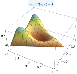
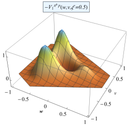
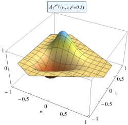
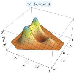
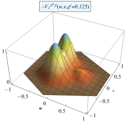
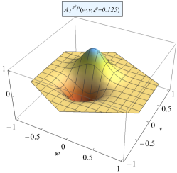
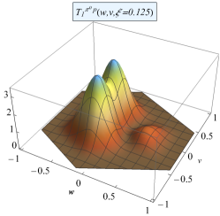
5.3 Nucleon-to-pion TDAs in the light-cone quark model

A clear physical interpretation for nucleon-to-meson TDAs can be obtained within the light-front quantization approach [190]. The basic notions of this framework are the light-front wave functions (LFWFs) of hadrons. They are expressed as expansions over various Fock components of hadronic states. For example, the LFWF of a nucleon or a meson state can be schematically represented by the following decompositions:

$$|N\rangle=\psi_{(3q)}|qqq\rangle+\psi_{(3q+1g)}|qqqg\rangle+\psi_{(3q+q\bar{q})}|qqqq\bar{q}\rangle+\cdots;{}$$

$$|{\mathcal{M}}\rangle=\psi_{(q\bar{q})}|q\bar{q}\rangle+\psi_{(q\bar{q}+1g)}|q\bar{q}g\rangle++\psi_{(q\bar{q}+q\bar{q})}|q\bar{q}q\bar{q}\rangle+\cdots\,.$$ (5.62)

Depending on the particular support region in longitudinal momentum fractions, ${\mathcal{M}}N$ TDAs give access to overlaps of the non-minimal Fock components of the nucleon and meson LFVFs, see Fig. 24. This provides additional information on the partonic correlations inside hadrons. In particular, in the ERBL-like region ${\mathcal{M}}N$ TDAs probe the non-minimal $(3q+q\bar{q})$ Fock component of the nucleon LFWF. Thus ${\mathcal{M}}N$ TDAs complement nucleon DAs that probe the lowest $3q$ Fock components of the nucleon LFWF.

Figure 24: Interpretation of nucleon-to-meson TDAs within the light-front quantization framework. Small vertical arrows show the direction of flow of longitudinal momenta. (a): Contribution in the ERBL-like region (all $x_{i}$ are positive); (b): Contribution in the DGLAP-like I region (one of $x_{i}$ is negative). (c): Contribution in the DGLAP-like II region (two $x_{i}$s are negative).

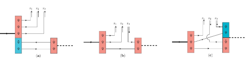
In Refs. [191, 192, 129] both leading twist-$3$ nucleon DAs and $\pi N$ TDAs were considered within a phenomenological model for LFWFs of the nucleon based on the light-cone constituent quark model. Previously, this model was successfully applied to the description of elastic form factors [193], parton distributions [194], GPDs [195] and transverse momentum dependent parton distribution functions (TMD PDFs) [196]. In Ref. [197] this model was applied to the calculation of collinear PDFs. In this subsection we present a short review of the key results of Refs. [191, 129] for $\pi N$ TDAs in the ERBL-like region.

The basic ingredients needed to compute the matrix elements $T^{s_{N}}_{\rho\tau,\,\chi}$ and express $\pi N$ TDAs in the ERBL-like region are the non-minimal five-quark ($qqqq\bar{q}$) component of a nucleon state and the valence $(q\bar{q})$ component of the pion state.

The five-quark component of a nucleon state was modeled within the meson-cloud model of Refs. [198, 199]. This model assumes that a physical nucleon consists of a bare nucleon dressed with a meson cloud. Thus the nucleon state is represented as a meson–baryon Fock expansion formed as a superposition of a three-valence-quark bare nucleon state and states containing virtual mesons with recoiling baryons. The baryon–meson subsystems include configurations with a nucleon or a $\Delta$-baryon accompanied with a pion as well as vector ($\rho$ and $\omega$) mesons. For the calculation of nucleon-to-pion TDAs it suffices to consider meson–baryon subsystems containing nucleon or $\Delta$ and a pion. This allows one to write the following dynamical representation:

$$|N(B\pi);p_{p},\lambda\rangle= \int\mathrm{d}y\mathrm{d}^{2}{\mathbf{k}}_{\perp}\int_{0}^{y}\left[\prod_{i=1}^{3}\frac{\mathrm{d}\xi_{i}}{\sqrt{\xi_{i}}}\right]\int_{0}^{(1-y)}\left[\prod_{i=4}^{5}\frac{\mathrm{d}\xi_{i}}{\sqrt{\xi_{i}}}\right]\int\frac{1}{\left[2(2\pi)^{3}\right]^{4}}\prod_{i=1}^{5}\mathrm{d}^{2}{\mathbf{k}}_{i\perp}^{\prime}$$ (5.63)

$$\times\delta\left(y-\sum_{i=1}^{3}\xi_{i}\right)\delta^{(2)}\left({\mathbf{k}}_{\perp}-\sum_{i=1}^{3}{\mathbf{k}}_{i\perp}^{\prime}\right)\delta\left(1-\sum_{i=1}^{5}\xi_{i}\right)\delta^{(2)}\left(\sum_{i=1}^{5}{\mathbf{k}}_{i\perp}^{\prime}\right)$$

$$\times\sum_{\lambda^{\prime}\lambda_{i},\tau_{i},c_{i}}\phi_{\lambda^{\prime}0}^{\lambda(N,B\pi)}\left(y,{\mathbf{k}}_{\perp}\right)\sqrt{y(1-y)}\tilde{\Psi}_{\lambda^{\prime}}^{B,[f]}\left(y,{\mathbf{k}}_{\perp};\left\{\xi_{i},{\mathbf{k}}_{i\perp}^{\prime};\lambda_{i},\tau_{i},c_{i}\right\}_{i=1,\ldots,3}\right)$$

$$\times\tilde{\Psi}^{\pi,[f]}\left(1-y,-{\mathbf{k}}_{\perp};\left\{\xi_{i},{\mathbf{k}}_{i\perp}^{\prime};\lambda_{i},\tau_{i}\right\}_{i=4,5}\right)\prod_{i=1}^{5}|\xi_{i}p_{p}^{+},{\mathbf{k}}_{i\perp}^{\prime}+\xi_{i}{\mathbf{p}}_{p\perp},\lambda_{i},\tau_{i},c_{i};q\rangle$$

The sum on the right-hand side of (5.63) stands over the baryon helicity $\lambda^{\prime}$, quark helicities $\lambda_{i}$, quark color indices $c_{i}$ and isotopic indices $\tau_{i}$; $\tilde{\Psi}_{\lambda^{\prime}}^{B,[f]}$ and $\tilde{\Psi}_{\lambda^{\prime}}^{\pi,[f]}$ denote the LFWFs of a baryon and a pion, respectively. The splitting function $\phi_{\lambda^{\prime}0}^{\lambda(N,B\pi)}(y,{\mathbf{k}}_{\perp})$ describes the probability amplitude to find a physical nucleon with helicity $\lambda$ in a state consisting of a virtual baryon $B=N,\,\Delta$ with helicity $\lambda^{\prime}$, longitudinal momentum fraction $y$ and transverse momentum ${\mathbf{k}}_{\bot}$ and the pion with longitudinal momentum fraction $1-y$ and transverse momentum $-{\mathbf{k}}_{\bot}$. These functions have been tabulated in Ref. [198].

For the pion state the valence $q\bar{q}$ component is considered

$$|\pi\left(p_{\pi}\right)\rangle=\sum_{\tau_{i},\lambda_{i},c_{i}}\int\prod_{i=1}^{2}\frac{\mathrm{d}\xi_{i}}{\sqrt{\xi_{i}}}\left[\prod_{i=1}^{2}\mathrm{d}^{2}{\mathbf{k}}_{i\perp}\right]\Psi^{\pi,[f]}\left(\left\{\xi_{i},\mathbf{k}_{i\perp};\lambda_{i},\tau_{i}\right\}_{i=1,2}\right)\prod_{i=1}^{2}|q^{\lambda_{i}};\xi_{i}p_{\pi}^{+},\mathbf{p}_{i\perp}\rangle,$$ (5.64)

where ${\mathbf{p}}_{\perp i}={\mathbf{k}}_{i\perp}+\xi_{i}{\mathbf{p}}_{\pi\bot}$.

Using the expressions (5.63), (5.64) together with the momentum representation for the quark fields and the set of anticommutation relations for the quark creation/annihilation operators one can establish the final expression for the matrix elements $T^{\lambda}_{\rho\tau,\,\chi}$ suitable for the calculation of $\pi N$ TDAs in the ERBL-like domain:

$$T_{\rho\tau,\,\chi}^{\lambda}= -24\left(\frac{1}{2\xi}\right)^{3/2}\frac{1}{\sqrt{x_{1}x_{2}x_{3}}}u_{+\rho}\left(k_{1}^{+},\lambda_{1}\right)u_{+\tau}\left(k_{2}^{+},\lambda_{2}\right)u_{+\chi}\left(k_{3}^{+},\lambda_{3}\right)$$ (5.65)

$$\times\sum_{B=N,\Delta}\sum_{\lambda^{\prime}}\int\mathrm{d}y\mathrm{d}^{2}{\mathbf{k}}_{\perp}\phi_{\lambda^{\prime}0}^{\lambda(N,B\pi)}\left(y,{\mathbf{k}}_{\perp}\right)\sqrt{y(1-y)}\delta\left(1-y-\frac{p_{\pi}^{+}}{p_{p}^{+}}\right)\delta^{(2)}\left({\mathbf{k}}_{\perp}+{\mathbf{p}}_{\pi\perp}\right)$$

$$\times\int\left[\prod_{i=1}^{3}{\mathbf{k}}_{i\perp}\right]\tilde{\Psi}_{\lambda^{\prime}}^{B,[f]}\left(\left\{\frac{x_{1}}{2\xi},{\mathbf{k}}_{1\perp};\lambda_{1},1/2\right\}\left\{\frac{x_{2}}{2\xi},{\mathbf{k}}_{2\perp};\lambda_{2},1/2\right\}\left\{\frac{x_{3}}{2\xi},{\mathbf{k}}_{3\perp};\lambda_{3},-1/2\right\}\right).$$

The quark light-cone spinors of the longitudinal momenta $k_{i}^{+}=x_{i}P^{+}$ in (5.65) are given by

$$u_{+}\left(x_{i}P^{+},\uparrow\right)=\sqrt{\frac{x_{i}P^{+}}{\sqrt{2}}}\left(\begin{array}[]{l}1\\ 0\\ 1\\ 0\end{array}\right)\quad\text{ and }\quad u_{+}\left(x_{i}P^{+},\downarrow\right)=\sqrt{\frac{x_{i}P^{+}}{\sqrt{2}}}\left(\begin{array}[]{c}0\\ 1\\ 0\\ -1\end{array}\right),\quad i=1,2,3.$$ (5.66)

Eq. (5.65) relates $\pi N$ TDAs to the baryon DAs in the $B\pi$ component of the nucleon weighted by the probability amplitude that the nucleon fluctuates in the corresponding subsystem with the pion momentum matching the pion momentum in the final state. The momentum fraction of the quarks in the baryon LFWF are defined with respect to the longitudinal momentum of the baryon. The integration over the transverse quark momenta corresponds to the projection of the baryon LFWF onto the zero orbital angular momentum component. The sum over the helicity $\lambda^{\prime}$ of the baryon permits baryon–pion fluctuations which do not conserve the helicity of the parent nucleon.

The explicit expression for the $uud$ isospin component of the nucleon and $\Delta$ wave functions $\Psi_{\lambda}^{p,[f]}\left(\left\{x_{i},\mathbf{k}_{i\perp};\lambda_{i}\right\},\{uud\}\right)$, $\Psi_{\lambda}^{\Delta,[f]}\left(\left\{x_{i},\mathbf{k}_{i\perp};\lambda_{i}\right\},\{uud\}\right)$ can be found in Secs. IV, V and Appendix A of Ref. [129]. Similarly to the calculation of nucleon DA, the model allows the calculation of $\pi N$ TDAs at a rather low normalization point $Q_{0}^{2}$.

Figure 25: The $N^{p}\to\pi^{0}$ TDAs $V_{1,2}^{p\pi^{0}}$, $A_{1,2}^{p\pi^{0}}$ computed in the model of Ref. [129] as functions of quark–diquark coordinates $w\equiv w_{3}$, $v\equiv v_{3}$ (4.45) in the ERBL-like domain for $\xi=0.9$, $\Delta^{2}=-0.1\leavevmode\nobreak\ {\rm GeV}^{2}$. Red lines show the borders of the ERBL-like support domain for $\xi=0.9$. Blue lines delimit the DGLAP-like support domains for $\xi=0.9$.

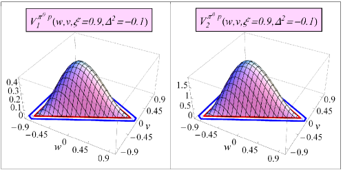
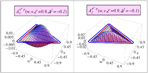
The resulting $8$ proton-to-$\pi^{0}$ TDAs are presented in Figs. 25, 26. They receive contribution from the fluctuations of the proton into $p\pi^{0}$ and $\Delta^{+}\pi^{0}$ subsystems. In particular, $\Delta$ plays a special role in the case of the tensor TDAs which involve configurations with helicity $\pm\frac{3}{2}$. The interplay of the nucleon and $\Delta$ contributions with helicity $\pm\frac{1}{2}$ determines the different shapes of the vector and axial-vector TDAs.

Figure 26: The $N^{p}\to\pi^{0}$ TDAs $T_{1,2,3,4}^{p\pi^{0}}$ computed in the model of Ref. [129] as functions of quark–diquark coordinates $w\equiv w_{3}$, $v\equiv v_{3}$ (4.45) in the ERBL-like domain for $\xi=0.9$, $\Delta^{2}=-0.1\leavevmode\nobreak\ {\rm GeV}^{2}$. Red lines show the borders of the ERBL-like support domain for $\xi=0.9$. Blue lines delimit the DGLAP-like support domains for $\xi=0.9$.

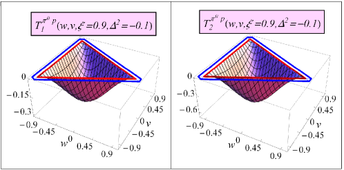
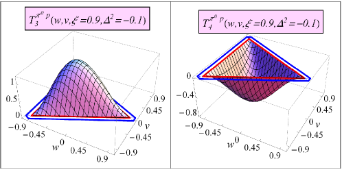
It is interesting to note that, similarly to the calculation of nucleon DAs in the same model, assuming the SU$(6)$ spin-flavor symmetry results in a shape of the $\pi N$ TDAs that repeats the shape of the asymptotic nucleon DA with a nearly symmetric contribution of the three quarks.

6 Exclusive processes involving TDAs to lowest order accuracy

The calculation of the lowest order in the strong coupling $\alpha_{s}$ and at the leading twist accuracy (LO) scattering amplitudes of hard exclusive reactions admitting a description in terms of nucleon-to-meson (and nucleon-to-photon) TDAs shares many common features with the textbook LO pQCD calculation of the nucleon electromagnetic form factor in terms of the leading twist-$3$ nucleon DAs. This section contains a summary of results for the relevant LO scattering amplitudes.

6.1 Nucleon form factor to the lowest order accuracy: a compact formula

The isospin parametrization for the nucleon DAs and nucleon-to-meson TDAs presented in Sec. 4.6 makes the calculations of the LO scattering amplitudes involving hadronic matrix element of the three-quark light-cone operator particularly simple. In this section we illustrate the application of this technique and present a new compact LO formula for the nucleon electromagnetic form factor.

Figure 27: Basic diagram for the calculation of the hard scattering kernel for the LO nucleon form factor. By crosses we mark the possible locations of insertion of the electromagnetic current $(\sigma_{\rm e.m.})^{f}_{\;i}=\frac{Q^{u}+Q^{d}}{2}\delta^{f}_{\;i}+\frac{Q^{u}-Q^{d}}{2}\sigma^{f}_{\;i}$, where $i$ ($f$) stand for the SU$(2)$-isospin indices of the incoming (outgoing) nucleon; $\rho,\,\tau,\chi$ ($\rho^{\prime},\,\tau^{\prime},\chi^{\prime}$) and $\alpha,\,\beta,\gamma$ ($\alpha^{\prime},\,\beta^{\prime},\gamma^{\prime}$) stand for the Dirac and SU$(2)$-isospin indices of the incoming (outgoing) quarks.

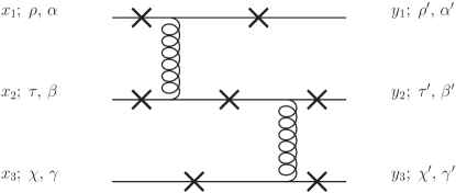
To describe the outgoing nucleon we use the following parametrization for the complex conjugated nucleon DA (4.102):

$$4\langle N_{f}(p)|\widehat{\bar{O}}_{\alpha\beta\gamma\;\rho\tau\chi}(1,2,3)|0\rangle\equiv 4\langle N_{f}(p)|\varepsilon_{c_{1}c_{2}c_{3}}\bar{\Psi}_{\rho\alpha}^{c_{1}}(1)\bar{\Psi}_{\tau\beta}^{c_{2}}(2)\bar{\Psi}_{\chi\gamma}^{c_{3}}(3)|0\rangle$$

$$=-\bigl{(}\varepsilon_{\alpha\beta}\delta_{\gamma}^{f}\overline{M}^{N\,\{13\}}_{\rho\tau\chi}(1,2,3)+\varepsilon_{\alpha\gamma}\delta_{\beta}^{f}\overline{M}^{N\,\{12\}}_{\rho\tau\chi}(1,2,3)\bigr{)}\,,$$ (6.1)

with

$$\overline{M}^{N\,\{12\}}_{\rho\tau\chi}(1,2,3)=f_{N}\Bigl{[}V^{p}(1,2,3)\bar{v}_{\rho\tau,\,\chi}^{N}+A^{p}(1,2,3)\bar{a}_{\rho\tau,\,\chi}^{N}+T^{p}(1,2,3)\bar{t}_{\rho\tau,\,\chi}^{N}\Bigr{]}$$ (6.2)

and

$$\overline{M}^{N\,\{13\}}_{\rho\tau\chi}(1,2,3)=\overline{M}^{N\,\{12\}}_{\rho\chi\tau}(1,3,2).$$ (6.3)

In (6.2) we employ the set of the conjugated Dirac structures $\bar{s}^{N}\equiv(s^{N}_{\rho^{\prime}\tau^{\prime}\chi^{\prime}})^{*}\gamma^{0}_{\rho^{\prime}\rho}\gamma^{0}_{\tau^{\prime}\tau}\gamma^{0}_{\chi^{\prime}\chi}$:

$$\bar{v}^{N}_{\rho\tau\chi}=(C^{\dagger}\hat{p})_{\tau\rho}(\bar{U}(p)\gamma_{5})_{\chi}\,;$$

$$\bar{a}^{N}_{\rho\tau\chi}=(C^{\dagger}\gamma^{5}\hat{p})_{\tau\rho}(\bar{U}(p))_{\chi}\,;$$

$$\bar{t}^{N}_{\rho\tau\chi}=(C^{\dagger}\sigma_{\mu p})_{\tau\rho}(\bar{U}(p)\gamma_{5}\gamma^{\mu})_{\chi}\,.$$ (6.4)

The $7$ diagrams needed to compute the nucleon form factor (FF) with our system of isospin notations are schematically presented in Fig. 27. The number of independent diagrams is further reduced to just $4$ (one of which is identically zero) due to the $C$-conjugation symmetry between the initial and final state nucleons. This represents a considerable simplification comparing to the original approach, in which $14$ independent diagrams have to be computed. In this way we obtain the following simple formula the proton and neutron form factor in terms of the leading twist-$3$ nucleon DA $\phi^{N}$:

$$Q^{4}F_{1}^{p,n}(Q^{2})=\frac{(4\pi\alpha_{s})^{2}}{54}f_{N}^{2}\int_{0}^{1}d_{3}x\;\delta\left(\sum_{l=1}^{3}x_{j}-1\right)\,\int_{0}^{1}d_{3}y\;\delta\left(\sum_{l=1}^{3}y_{l}-1\right)\left\{2(R_{1}^{p,n}+R_{2}^{p,n}+R_{3}^{p,n})+R_{4}^{p,n}\right\},$$ (6.5)

where $\alpha_{s}$ is the strong coupling and $f_{N}$ is the nucleon light-cone wave function normalization constant. Ref. [25] quotes the following value for $f_{N}$:

$$f_{N}=5.0\cdot 10^{-3}\;{\rm GeV}^{2}.$$ (6.6)

The integration in (6.5) stands over the usual support of nucleon DAs

$$\int_{0}^{1}d_{3}x\;\delta\left(\sum_{l=1}^{3}x_{j}-1\right)\,\int_{0}^{1}d_{3}y\;\delta\left(\sum_{l=1}^{3}y_{l}-1\right){}$$

$$\equiv\int_{0}^{1}dx_{1}dx_{2}dx_{3}\delta(x_{1}+x_{2}+x_{3}-1)\int_{0}^{1}dy_{1}dy_{2}dy_{3}\delta(y_{1}+y_{2}+y_{3}-1).$$ (6.7)

The integrands $R_{\alpha}^{\{p,n\}}$ in (6.5) have the following structure (no summation is implied over the repeating index $\alpha$):

$$R_{\alpha}^{\{p,n\}}=D_{\alpha}N_{\alpha}^{\{p,n\}},$$ (6.8)

where $D_{\alpha}$ stand for the hard convolution kernels originating from the partonic propagators and $N_{\alpha}^{\{p,n\}}$ are combinations of nucleon DAs. The explicit expressions for the denominators $D_{\alpha}$ and numerators $N_{\alpha}^{\{p,n\}}$ are summarized in Table LABEL:Table_Nucl_FF.

Table 3: Differential cross section $\frac{d\sigma}{d\Delta^{2}}$ for $p\bar{p}\to J/\psi\,\pi^{0}$ as a function of $\Delta_{T}^{2}$ for $W^{2}=15\leavevmode\nobreak\ {\rm GeV}^{2}$ (left panel) and $W^{2}=20\leavevmode\nobreak\ {\rm GeV}^{2}$ (right panel). [Reprinted Figure 4 from Ref. [22]. Copyright (2013) by Elsevier.]

$\alpha$	Diagram	Numerators
	$D_{\alpha}$
1			$\frac{1}{(1-x_{1})^{2}x_{3}\,(1-y_{1})^{2}y_{3}}$	$N_{\alpha}^{p}$ $\frac{1}{3}\left(2\phi^{N}(x_{1},x_{2},x_{3})+\phi^{N}(x_{3},x_{2},x_{1})\right)\left(2\phi^{N}(y_{1},y_{2},y_{3})+\phi^{N}(y_{3},y_{2},y_{1})\right)$ $+\frac{1}{3}\left(2\phi^{N}(x_{1},x_{3},x_{2})+\phi^{N}(x_{2},x_{3},x_{1})\right)\left(2\phi^{N}(y_{1},y_{3},y_{2})+\phi^{N}(y_{2},y_{3},y_{1})\right);$ $N_{\alpha}^{n}$ $\frac{1}{3}\left(\phi^{N}(x_{1},x_{3},x_{2})-\phi^{N}(x_{2},x_{3},x_{1})\right)\left(\phi^{N}(y_{1},y_{3},y_{2})-\phi^{N}(y_{2},y_{3},y_{1})\right)$ $+\frac{1}{3}\left(\phi^{N}(x_{3},x_{2},x_{1})-\phi^{N}(x_{1},x_{2},x_{3})\right(\left(\phi^{N}(y_{3},y_{2},y_{1})-\phi^{N}(y_{1},y_{2},y_{3})\right)$ $-\phi^{N}(x_{1},x_{2},x_{3})\phi^{N}(y_{1},y_{2},y_{3})-\phi^{N}(x_{1},x_{3},x_{2})\phi^{N}(y_{1},y_{3},y_{2});$
2		$N_{\alpha}^{p}$ $0;$ $N_{\alpha}^{n}$ $0;$
3	$\frac{1}{x_{1}(1-x_{2})x_{3}\,y_{1}(1-y_{1})y_{3}}$	$N_{\alpha}^{p}$ $-\frac{1}{3}\left(\phi^{N}(x_{1},x_{3},x_{2})+2\phi^{N}(x_{2},x_{3},x_{1})\right)\left(\phi^{N}(y_{1},y_{3},y_{2})+2\phi^{N}(y_{2},y_{3},y_{1})\right);$ $N_{\alpha}^{n}$ $-\frac{1}{3}\left(\phi^{N}(x_{2},x_{3},x_{1})-\phi^{N}(x_{1},x_{3},x_{2})\right)\left(\phi^{N}(y_{2},y_{3},y_{1})-\phi^{N}(y_{1},y_{3},y_{2})\right)$ $+\phi^{N}(x_{2},x_{3},x_{1})\phi^{N}(y_{2},y_{3},y_{1});$
4	$\frac{1}{x_{1}x_{3}(1-x_{3})\,y_{1}(1-y_{1})y_{3}}$	$N_{\alpha}^{p}$ $\frac{1}{3}\left(\phi^{N}(x_{1},x_{2},x_{3})-\phi^{N}(x_{3},x_{2},x_{1})\right)\left(\phi^{N}(y_{1},y_{2},y_{3})-\phi^{N}(y_{3},y_{2},y_{1})\right);$ $N_{\alpha}^{n}$ $\frac{1}{3}\left(\phi^{N}(x_{1},x_{2},x_{3})+2\phi^{N}(x_{3},x_{2},x_{1})\right)\left(\phi^{N}(y_{1},y_{2},y_{3})+2\phi^{N}(y_{3},y_{2},y_{1})\right)$ $-\phi^{N}(x_{3},x_{2},x_{1})\phi^{N}(y_{3},y_{2},y_{1});$

• With the use of the asymptotic form of the nucleon DA $\phi^{N}_{\rm as}(x_{1},x_{2},x_{3})=120x_{1}x_{2}x_{3}$ we recover the result of [200]:

  $$Q^{4}F_{1}^{p}(Q^{2})\Big{|}_{\phi^{N}_{\rm as}}=0;\ \ \ Q^{4}F_{1}^{n}(Q^{2})\Big{|}_{\phi^{N}_{\rm as}}=\frac{(4\pi\alpha_{s})^{2}f_{N}^{2}}{54}1.8\cdot 10^{3}.$$ (6.9)

• With the use of the COZ phenomenological solution of  [25]

  $$\phi^{N}_{\rm COZ}(x_{1},\,x_{2},\,x_{3})=\phi^{N}_{\rm as}(x_{1},\,x_{2},\,x_{3})\left[23.814x_{1}^{2}+12.978x_{2}^{2}+6.174x_{3}^{2}+5.88x_{3}-7.098\right]$$ (6.10)

  we recover the result of Ref. [25] both for the proton and neutron FFs. In particular,

  $$Q^{4}F_{1}^{p}(Q^{2})\Big{|}_{\phi^{N}_{\rm COZ}}=\frac{(4\pi\alpha_{s})^{2}f_{N}^{2}}{54}\,1.45\cdot 10^{5};\ \ \ \frac{F_{1}^{n}\left(Q^{2}\right)}{F_{1}^{p}\left(Q^{2}\right)}\Big{|}_{\phi^{N}_{\rm COZ}}\simeq-0.47.$$

We would like to attract the attention of the reader to a possible controversy in the normalization of the proton helicity $\uparrow$ state (and hence of the nucleon DA $\phi^{N}$) first reported in Ref. [201]. It was considered by different authors [202, 203] (see particularly the discussion in Sec. III.C of Ref. [203]). A dedicated study in Ref. [200] has confirmed the consistency of the conventions employed by V. Chernyak [25] (see also Ref. [204]). Throughout our analysis we rely on this latter set of conventions.

6.2 Backward meson electroproduction: calculation of the hard amplitude

In this section we present the calculation of the leading-twist leading order in $\alpha_{s}$ scattering amplitudes of backward hard meson electroproduction reactions within the collinear factorization approach involving description in terms of nucleon DAs and nucleon-to-meson TDAs.

6.2.1 Backward pseudoscalar meson electroproduction

Let us first address the pseudoscalar meson case, and for definiteness consider hard backward pion electroproduction:

$$\gamma^{*}(q,\lambda_{\gamma})+N(p_{N},s_{N})\to N(p^{\prime}_{N},s^{\prime}_{N})+\pi(p_{\pi})$$ (6.11)

in the near-backward kinematical regime (see Sec. 3.1). This requires the calculation of the same set of $21$ diagrams as the leading twist-$3$, leading order in $\alpha_{s}$ calculation of the nucleon electromagnetic form factor.

For the phenomenological applications it turns out to be convenient to employ the parametrization of the leading twist-$3$ $\pi N$ TDAs introduced in Sec. 4.1.1 with the set of the Dirac structures (4.6) explicitly depending on $\Delta_{T}$. This allows a clear separation of the $\Delta_{T}$-dependent and $\Delta_{T}$-independent contributions to the amplitude of the reaction (LABEL:Reaction_ampl_p_pi0), the latter controlling the only surviving contributions in the strictly backward kinematical regime $\Delta_{T}=0$.

To the leading twist-$3$, leading order in $\alpha_{s}$ accuracy, the helicity amplitudes ${\mathcal{M}}_{s_{N}s^{\prime}_{N}}^{\lambda_{\gamma}}$ of the reaction (LABEL:Reaction_ampl_p_pi0) admit the following parametrization

$${\mathcal{M}}_{s_{N}s^{\prime}_{N}}^{\lambda_{\gamma}}={\mathcal{C}}_{\pi}\frac{1}{Q^{4}}\sum_{k=1}^{2}{\mathcal{S}}_{s_{N}s^{\prime}_{N}}^{(k)\,\lambda_{\gamma}}{\mathcal{I}}^{(k)}(\xi,\,\Delta^{2})\,,$$ (6.12)

with the overall normalization constant

$${\mathcal{C}}_{\pi}\equiv-i\frac{(4\pi\alpha_{s})^{2}\sqrt{4\pi\alpha_{em}}f_{N}^{2}}{54f_{\pi}},$$ (6.13)

where $\alpha_{em}\simeq\frac{1}{137}$ is the electromagnetic fine structure constant, $\alpha_{s}$ is the strong coupling, $f_{N}$ is the nucleon light-cone wave function normalization constant (6.6) and $f_{\pi}=93\leavevmode\nobreak\ {\rm MeV}$ is the pion weak decay constant.

The parametrization (LABEL:Hel_ampl_def_piN) involves two leading twist-$3$ spin structures ${\mathcal{S}}^{(1,2)\,\lambda_{\gamma}}_{s_{N}s^{\prime}_{N}}$ defined as

$${\mathcal{S}}^{(1)\,\lambda_{\gamma}}_{s_{N}s^{\prime}_{N}}\equiv\bar{U}(p^{\prime}_{N},s^{\prime}_{N})\hat{\mathcal{E}}(q,\lambda_{\gamma})\gamma^{5}U(p_{N},s_{N})\,;{}$$

$${\mathcal{S}}^{(2)\,\lambda_{\gamma}}_{s_{N}s^{\prime}_{N}}\equiv\frac{1}{m_{N}}\bar{U}(p^{\prime}_{N},s^{\prime}_{N})\hat{\mathcal{E}}(q,\lambda_{\gamma})\hat{\Delta}_{T}\gamma^{5}U(p_{N},s_{N}).$$ (6.14)

For the integral convolutions $\mathcal{I}^{(k=1,2)}$ in (LABEL:Hel_ampl_def_piN) we employ the following notations

$$\mathcal{I}^{(k)}(\xi,\Delta^{2})={\int^{1+\xi}_{-1+\xi}}\!\!\!d_{3}x\;\delta\left(\sum_{j=1}^{3}x_{j}-2\xi\right){\int^{1}_{0}}\!\!\!d_{3}y\;\delta\left(\sum_{l=1}^{3}y_{l}-1\right)\;{\Biggl{(}2\sum_{\alpha=1}^{7}T_{\alpha}^{(k)}+\sum_{\alpha=8}^{14}T_{\alpha}^{(k)}\Biggr{)}}.$$ (6.15)

The integration in (LABEL:Def_I_k_convolutions) stands over the support domain of $\pi N$ TDAs in the longitudinal momentum fraction variables $x_{i}$ and over the support domain of nucleon DAs in the longitudinal momentum fraction variables $y_{i}$:

$${\int^{1+\xi}_{-1+\xi}}\!\!\!d_{3}x\;\delta\left(\sum_{j=1}^{3}x_{j}-2\xi\right)\equiv{\int^{1+\xi}_{-1+\xi}}\!\!\!dx_{1}{\int^{1+\xi}_{-1+\xi}}\!\!\!dx_{2}{\int^{1+\xi}_{-1+\xi}}\!\!\!dx_{3}\delta(x_{1}+x_{2}+x_{3}-2\xi);$$

$${\int^{1}_{0}}\!\!\!d_{3}y\;\delta\left(\sum_{l=1}^{3}y_{l}-1\right)\equiv{\int^{1}_{0}}dy_{1}{\int^{1}_{0}}dy_{2}{\int^{1}_{0}}dy_{3}\delta(y_{1}+y_{2}+y_{3}-1).$$ (6.16)

The index $\alpha$ refers to the number of a diagram (see Table LABEL:Table_Bkw_pion) and the index $k=1,\,2$ runs for the contributions into the two invariant amplitudes of Eq. (LABEL:Hel_ampl_def_piN).

The general structure of the convolution integrals (LABEL:Def_I_k_convolutions) resembles much the familiar expressions for the leading twist hard amplitudes of hard exclusive meson electroproduction off nucleons within the collinear factorized description in terms of nucleon GPDs ($H(x,\xi)$) and meson DAs ($\phi_{\mathcal{M}}$) [12]:

$${\mathcal{A}}\Big{|}_{\text{HMP}}\sim\int_{-1}^{1}dx\frac{H(x,\xi)}{x\pm\xi\mp i0}\int_{0}^{1}dy\frac{\phi_{\mathcal{M}}(y)}{y}.$$ (6.17)

The coefficients $T_{\alpha}^{(k)}$ can be represented as products of singular hard kernels, originating from the partonic propagators, times the combinations $N_{\alpha}^{(k)}\equiv N_{\alpha}^{(k)}(x_{1},x_{2},\xi,\Delta^{2};\,y_{1},y_{2},y_{3})$ of $\pi N$ TDAs and nucleon DAs arising in the numerators:

$$T_{\alpha}^{(k)}\equiv D_{\alpha}\times N_{\alpha}^{(k)}.$$ (6.18)

Note that no summation over the repeating index $\alpha$ is assumed in (LABEL:Def_T_alpha).

• The explicit expressions for $T_{\alpha}^{(k)}$ $\alpha=1,\ldots,14$ for $\gamma^{*}N^{p}\to\pi^{0}N^{p}$ reaction are presented in Table LABEL:Table_Bkw_pion. We adopt the shortened notations for the arguments of $\pi N$ TDAs and nucleon DAs:

  $$\left\{V_{1,2}^{\pi^{0}p},\,A_{1,2}^{\pi^{0}p},\,T_{1,2,3,4}^{\pi^{0}p}\right\}\equiv\left\{V_{1,2}^{\pi^{0}p},\,A_{1,2}^{\pi^{0}p},\,T_{1,2,3,4}^{\pi^{0}p}\right\}(x_{1},x_{2},x_{3},\xi,\Delta^{2});{}$$

  $$\left\{V^{p},\,A^{p},\,T^{p}\right\}\equiv\left\{V^{p},\,A^{p},\,T^{p}\right\}(y_{1},y_{2},y_{3}).$$ (6.19)

  The diagrams with $\alpha=15,\ldots,21$ differ from those with $\alpha=1,\ldots,7$ by a permutation of the $u$-quark lines $1$ and $2$. They give the same contribution due to the symmetry of the integration domain and of the TDAs and DAs with respect to the change of variables $x_{1}\leftrightarrow x_{2}$, $y_{1}\leftrightarrow y_{2}$. Therefore, the diagrams with $\alpha=15,\ldots,21$ are accounted for by the factor $2$ in the last line of Eq. (LABEL:Def_I_k_convolutions).

• The result for $\gamma^{*}p\rightarrow\pi^{+}n$ channel can be read from the same Table LABEL:Table_Bkw_pion with the obvious changes:

  $$Q_{u}\rightarrow Q_{d};\ \ \ Q_{d}\rightarrow Q_{u}\,;$$

  $$V^{p},\,A^{p},\,T^{p}\,\rightarrow\,V^{n},\,A^{n},\,T^{n}\;\equiv-V^{p},\,-A^{p},\,-T^{p}\,;$$

  $$V^{\pi^{0}p}_{1,2},\,A^{\pi^{0}p}_{1,2},\,T^{\pi^{0}p}_{1,2,3,4}\,\rightarrow V^{\pi^{+}p}_{1,2},\,A^{\pi^{+}p}_{1,2},\,T^{\pi^{+}p}_{1,2,3,4}\,.$$ (6.20)

• The result presented in Table LABEL:Table_Bkw_pion can be also adopted for other pseudoscalar mesons. E.g. for $\eta$-meson one just has to replace the corresponding TDAs

  $$V^{\pi^{0}p}_{1,2},\,A^{\pi^{0}p}_{1,2},\,T^{\pi^{0}p}_{1,2,3,4}\,\rightarrow V^{\eta p}_{1,2},\,A^{\eta p}_{1,2},\,T^{\eta p}_{1,2,3,4}\,.$$ (6.21)

Table 3: Differential cross section $\frac{d\sigma}{d\Delta^{2}}$ for $p\bar{p}\to J/\psi\,\pi^{0}$ as a function of $\Delta_{T}^{2}$ for $W^{2}=15\leavevmode\nobreak\ {\rm GeV}^{2}$ (left panel) and $W^{2}=20\leavevmode\nobreak\ {\rm GeV}^{2}$ (right panel). [Reprinted Figure 4 from Ref. [22]. Copyright (2013) by Elsevier.]

$\alpha$	Diagram	Numerators
	$D_{\alpha}$
1			$\frac{Q_{u}(2\xi)^{2}}{(2\xi-x_{1}-i0)^{2}(x_{3}-i0)(1-y_{1})^{2}y_{3}}$	$N_{\alpha}^{(1)}$ $-\left(V^{p}-A^{p}\right)\left(V_{1}^{p\pi^{0}}-A_{1}^{p\pi^{0}}\right)-4T^{p}\left(T_{1}^{p\pi^{0}}+\frac{\Delta_{T}^{2}}{2m_{N}^{2}}T_{4}^{p\pi^{0}}\right);$ $N_{\alpha}^{(2)}$ $-\left(V^{p}-A^{p}\right)\left(V_{2}^{p\pi^{0}}-A_{2}^{p\pi^{0}}\right)-2T^{p}\left(T_{2}^{p\pi^{0}}+T_{3}^{p\pi^{0}}\right);$
2		$N_{\alpha}^{(1)}$ $0;$ $N_{\alpha}^{(2)}$ $0;$
3	$\frac{Q_{u}(2\xi)^{2})}{(x_{1}-i0)(2\xi-x_{2}-i0)(x_{3}-i0)y_{1}(1-y_{1})y_{3}}$	$N_{\alpha}^{(1)}$ $4T^{p}\left(T_{1}^{p\pi^{0}}+\frac{\Delta_{T}^{2}}{2m_{N}^{2}}T_{4}^{p\pi^{0}}\right);$ $N_{\alpha}^{(2)}$ $2T^{p}\left(T_{2}^{p\pi^{0}}+T_{3}^{p\pi^{0}}\right);$
4	$\frac{Q_{u}(2\xi)^{2}}{(x_{1}-i0)(2\xi-x_{3}-i0)(x_{3}-i0)y_{1}(1-y_{1})y_{3}}$	$N_{\alpha}^{(1)}$ $-\left(V^{p}-A^{p}\right)\left(V_{1}^{p\pi^{0}}-A_{1}^{p\pi^{0}}\right);$ $N_{\alpha}^{(2)}$ $-\left(V^{p}-A^{p}\right)\left(V_{2}^{p\pi^{0}}-A_{2}^{p\pi^{0}}\right);$
5	$\frac{Q_{u}(2\xi)^{2}}{(x_{1}-i0)(2\xi-x_{3}-i0)(x_{3}-i0)y_{1}(1-y_{2})y_{3}}$	$N_{\alpha}^{(1)}$ $\left(V^{p}+A^{p}\right)\left(V_{1}^{p\pi^{0}}+A_{1}^{p\pi^{0}}\right);$ $N_{\alpha}^{(2)}$ $\left(V^{p}+A^{p}\right)\left(V_{2}^{p\pi^{0}}+A_{2}^{p\pi^{0}}\right);$
6		$N_{\alpha}^{(1)}$ $0;$ $N_{\alpha}^{(2)}$ $0;$
7	$\frac{Q_{d}(2\xi)^{2}}{(x_{1}-i0)(2\xi-x_{3}-i0)^{2}y_{1}(1-y_{3})^{2}}$	$N_{\alpha}^{(1)}$ $-2\left(V^{p}V_{1}^{p\pi^{0}}+A^{p}A_{1}^{p\pi^{0}}\right);$ $N_{\alpha}^{(2)}$ $-2\left(V^{p}V_{2}^{p\pi^{0}}+A^{p}A_{2}^{p\pi^{0}}\right);$
8		$N_{\alpha}^{(1)}$ $0;$ $N_{\alpha}^{(2)}$ $0;$
9	$\frac{Q_{u}(2\xi)^{2}}{(2\xi-x_{1}-i0)^{2}(x_{2}-i0)(1-y_{1})^{2}y_{2}}$	$N_{\alpha}^{(1)}$ $-\left(V^{p}-A^{p}\right)\left(V_{1}^{p\pi^{0}}-A_{1}^{p\pi^{0}}\right)-4T^{p}\left(T_{1}^{p\pi^{0}}+\frac{\Delta_{T}^{2}}{2m_{N}^{2}}T_{4}^{p\pi^{0}}\right);$ $N_{\alpha}^{(2)}$ $-\left(V^{p}-A^{p}\right)\left(V_{2}^{p\pi^{0}}-A_{2}^{p\pi^{0}}\right)-2T^{p}\left(T_{2}^{p\pi^{0}}+T_{3}^{p\pi^{0}}\right);$
10	$\frac{Q_{u}(2\xi)^{2}}{(x_{1}-i0)(2\xi-x_{2}-i0)^{2}y_{1}(1-y_{2})^{2}}$	$N_{\alpha}^{(1)}$ $-\left(V^{p}+A^{p}\right)\left(V_{1}^{p\pi^{0}}+A_{1}^{p\pi^{0}}\right)-4T^{p}\left(T_{1}^{p\pi^{0}}+\frac{\Delta_{T}^{2}}{2m_{N}^{2}}T_{4}^{p\pi^{0}}\right);$ $N_{\alpha}^{(2)}$ $-\left(V^{p}+A^{p}\right)\left(V_{2}^{p\pi^{0}}+A_{2}^{p\pi^{0}}\right)-2T^{p}\left(T_{2}^{p\pi^{0}}+T_{3}^{p\pi^{0}}\right);$
11		$N_{\alpha}^{(1)}$ $0;$ $N_{\alpha}^{(2)}$ $0;$
12	$\frac{Q_{d}(2\xi)^{2}}{(x_{1}-i0)(x_{2}-i0)(2\xi-x_{3}-i0)y_{1}(1-y_{2})y_{2}}$	$N_{\alpha}^{(1)}$ $\left(V^{p}+A^{p}\right)\left(V_{1}^{p\pi^{0}}+A_{1}^{p\pi^{0}}\right);$ $N_{\alpha}^{(2)}$ $\left(V^{p}+A^{p}\right)\left(V_{2}^{p\pi^{0}}+A_{2}^{p\pi^{0}}\right);$
13	$\frac{Q_{d}(2\xi)^{2})}{(x_{1}-i0)(2\xi-x_{1}-i0)(x_{2}-i0)y_{1}(1-y_{2})y_{2}}$	$N_{\alpha}^{(1)}$ $-4T^{p}\left(T_{1}^{p\pi^{0}}+\frac{\Delta_{T}^{2}}{2m_{N}^{2}}T_{4}^{p\pi^{0}}\right);$ $N_{\alpha}^{(2)}$ $-2T^{p}\left(T_{2}^{p\pi^{0}}+T_{3}^{p\pi^{0}}\right);$
14	$\frac{Q_{d}(2\xi)^{2}}{(x_{1}-i0)(2\xi-x_{1}-i0)(x_{2}-i0)y_{1}y_{2}(1-y_{3})}$	$N_{\alpha}^{(1)}$ $\left(V^{p}-A^{p}\right)\left(V_{1}^{p\pi^{0}}-A_{1}^{p\pi^{0}}\right);$ $N_{\alpha}^{(2)}$ $\left(V^{p}-A^{p}\right)\left(V_{2}^{p\pi^{0}}-A_{2}^{p\pi^{0}}\right);$

We note that the $x_{i}$- and $y_{i}$- dependencies of the hard kernels $D_{\alpha}$ (LABEL:Def_T_alpha) are factorized:

$$D_{\alpha}\sim K_{\alpha}(x_{1},x_{2},x_{3},\xi)\,{\mathcal{K}}_{\alpha}(y_{1},y_{2},y_{3}).$$ (6.22)

• The hard kernels ${\mathcal{K}}_{\alpha}(y_{1},y_{2},y_{3})$ are similar to those occurring within the perturbative description of the nucleon electromagnetic form factor. The convolutions of nucleon DAs with ${\mathcal{K}}_{\alpha}(y_{1},y_{2},y_{3})$ do not produce any imaginary part for the amplitude since the nucleon DAs have pure ERBL support and are supposed to vanish at the borders of their domain of definition.

• To deal with the hard kernels $K_{\alpha}(x_{1},x_{2},x_{3},\xi)$ it turns out to be convenient to switch to the quark–diquark coordinates (see Sec. 4.3). For each diagram there exists a preferred choice $i=1,\,2,\,3$ of the quark–diquark coordinates $(w_{i},\,v_{i})$ (4.45) in which the corresponding convolution kernel $K_{\alpha}$ reduces to one of the following types

  $$K_{I}^{(\pm,\pm)}(w_{i},v_{i})=\frac{1}{(w_{i}\pm\xi\mp i0)}\frac{1}{(v_{i}\pm\xi^{\prime}_{i}\mp i0)},$$

  $$K_{II}^{(-,\pm)}(w_{i},v_{i})=\frac{1}{(w_{i}-\xi+i0)^{2}}\frac{1}{(v_{i}\pm\xi^{\prime}_{i}\mp i0)}.$$ (6.23)

  The singularities of the hard kernels (LABEL:Kernels_K) are located on the cross-over trajectories $w_{i}=-\xi,\,v_{i}=\pm\xi^{\prime}$ separating the ERBL-like and the DGLAP-like support domains of $\pi N$ TDAs and on the lines $w_{i}=\xi$ that belong to the DGLAP-like support domains. Thus the convolution integrals in $x_{i}$ with $\pi N$ TDAs in (LABEL:Def_I_k_convolutions) may generate a nonzero imaginary part for the amplitude. $\pi N$ TDAs, indeed, do not necessarily vanish on the cross over trajectories $x_{i}=0$, separating ERBL-like and DGLAP-like regimes, as well as on the lines $x_{i}=2\xi$.

We conclude that the calculation of the real and imaginary parts of $\mathcal{I}^{(k)}(\xi,\Delta^{2})$ requires the consideration of the two types of integral convolutions of TDAs:

$$I_{I}^{(\pm,\pm)}(\xi)=\int_{-1}^{1}dw\int_{-1+|\xi-\xi^{\prime}|}^{1-|\xi-\xi^{\prime}|}dv\frac{1}{(w\pm\xi\mp i0)}\frac{1}{(v\pm\xi^{\prime}\mp i0)}H(w,v,\xi),$$ (6.24)

and

$$I_{II}^{(-,\pm)}(\xi)=\int_{-1}^{1}dw\int_{-1+|\xi-\xi^{\prime}|}^{1-|\xi-\xi^{\prime}|}dv\frac{1}{(w-\xi+i0)^{2}}\frac{1}{(v\pm\xi^{\prime}\mp i0)}H(w,v,\xi).$$ (6.25)

In Eqs. (LABEL:I_I), (LABEL:I_II) we adopt the convention that the first sign in the $(\pm,\pm)$ index of a quantity corresponds to the sign in the $w\pm\xi$ denominator while the second sign in the index corresponds to the sign in the $v\pm\xi^{\prime}$ denominator. The real and imaginary parts of the integral convolutions (LABEL:I_I), (LABEL:I_II) presented in Ref. [19] contain some misprints and sign errors. The revised expressions are summarized in App. LABEL:App_Conv_Re_Im.

6.2.2 Backward vector meson electroproduction

In this subsection, using generally the same system of notations as in Sec. LABEL:SubSec_Ampl_Pkw_PS_meson, we present the leading twist leading order in $\alpha_{s}$ amplitude of backward vector meson hard electroproduction reaction

$$\gamma^{*}(q,\lambda_{\gamma})+N(p_{N},s_{B})\to N(p^{\prime}_{N},s^{\prime}_{N})+V(p_{V},\lambda_{V}).$$ (6.26)

within the collinear factorized description in terms of nucleon DAs and nucleon-to-vector meson TDAs (4.13).

The corresponding helicity amplitudes involve $6$ independent tensor structures

$${\mathcal{M}}_{s_{N}s^{\prime}_{N}}^{\lambda_{\gamma}\lambda_{V}}={\mathcal{C}}_{V}\frac{1}{Q^{4}}\sum_{k=1}^{6}{\mathcal{S}}_{s_{N}s^{\prime}_{N}}^{(k)\,\lambda_{\gamma}\lambda_{V}}{\mathcal{I}}^{(k)}(\xi,\,\Delta^{2}),$$ (6.27)

where the overall normalization constant ${\mathcal{C}}_{V}$ reads

$${\mathcal{C}}_{V}=-i\frac{(4\pi\alpha_{s})^{2}\sqrt{4\pi\alpha_{em}}f_{N}m_{N}}{54}.$$ (6.28)

There turns out to be $2$ tensor structures independent of $\Delta_{T}$:

$${\mathcal{S}}_{s_{N}s^{\prime}_{N}}^{(1)\,\lambda_{\gamma}\lambda_{V}}=\bar{U}(p^{\prime}_{N},s^{\prime}_{N})\hat{\mathcal{E}}(q,\lambda_{\gamma})\hat{\mathcal{E}}^{*}(p_{V},\lambda_{V})U(p_{N},s_{N});$$

$${\mathcal{S}}_{s_{N}s^{\prime}_{N}}^{(2)\,\lambda_{\gamma}\lambda_{V}}=m_{N}({\mathcal{E}}^{*}(p_{V},\lambda_{V})\cdot n)\bar{U}(p^{\prime}_{N},s^{\prime}_{N})\hat{\mathcal{E}}(q,\lambda_{\gamma})U(p_{N},s_{N}),$$ (6.29)

and $4$ $\Delta_{T}$-dependent tensor structures:

$${\mathcal{S}}_{s_{N}s^{\prime}_{N}}^{(3)\,\lambda_{\gamma}\lambda_{V}}=\frac{1}{m_{N}}({\mathcal{E}}^{*}(p_{V},\lambda_{V})\cdot\Delta_{T})\,\bar{U}(p^{\prime}_{N},s^{\prime}_{N})\hat{\mathcal{E}}(q,\lambda_{\gamma})U(p_{N},s_{N});$$

$${\mathcal{S}}_{s_{N}s^{\prime}_{N}}^{(4)\,\lambda_{\gamma}\lambda_{V}}=\frac{1}{m_{N}^{2}}({\mathcal{E}}^{*}(p_{V},\lambda_{V})\cdot\Delta_{T})\,\bar{U}(p^{\prime}_{N},s^{\prime}_{N})\hat{\mathcal{E}}(q,\lambda_{\gamma})\hat{\Delta}_{T}U(p_{N},s_{N});$$

$${\mathcal{S}}_{s_{N}s^{\prime}_{N}}^{(5)\,\lambda_{\gamma}\lambda_{V}}=\frac{1}{m_{N}}\,\bar{U}(p^{\prime}_{N},s^{\prime}_{N})\hat{\mathcal{E}}(q,\lambda_{\gamma})\hat{{\mathcal{E}}}^{*}(p_{V},\lambda_{V})\hat{\Delta}_{T}U(p_{N},s_{N});$$

$${\mathcal{S}}_{s_{N}s^{\prime}_{N}}^{(6)\,\lambda_{\gamma}\lambda_{V}}=({\mathcal{E}}^{*}(p_{V},\lambda_{V})\cdot n)\,\bar{U}(p^{\prime}_{N},s^{\prime}_{N})\hat{\mathcal{E}}(q,\lambda_{\gamma})\hat{{\mathcal{E}}}^{*}(p_{V},\lambda_{V})\hat{\Delta}_{T}U(p_{N},s_{N}).$$ (6.30)

Here $\mathcal{E}(q,\lambda_{\gamma})$ stands for the polarization vector of the incoming virtual photon and ${\mathcal{E}}^{*}(p_{V},\lambda_{V})$ is the polarization vector of the outgoing vector meson.

To the leading order in $\alpha_{s}$, within the collinear factorized description in terms of nucleon DAs and $VN$ TDAs, the amplitude of the reaction (LABEL:reaction_amp) can be computed from the same $21$ diagrams as listed in Table LABEL:Table_Bkw_pion.

For definiteness we take $V$ to be a neutral vector meson $\omega$, $\rho^{0}$ or $\phi$ and present the results for $\gamma^{*}N^{p}\to N^{p}V^{0}$ channel. We adopt the common notations for the integral convolutions (LABEL:Def_I_k_convolutions) $\mathcal{I}^{(k)}(\xi,\Delta^{2})$, $k=1,\,\ldots,\,6$. The explicit expressions for the corresponding coefficients $T_{\alpha}^{(k)}\equiv D_{\alpha}\times N_{\alpha}^{(k)}$ (no summation over $\alpha$ assumed) are presented in Table LABEL:Table_Bkw_vector. The singular kernels $D_{\alpha}$ turn out to be the same as in the pseudoscalar meson case and $N_{\alpha}^{(k)}\equiv N_{\alpha}^{(k)}(x_{1},x_{2},x_{3},\xi,\Delta^{2};\,y_{1},y_{2},y_{3})$ stand for the appropriate combinations of $VN$ TDAs and nucleon DAs $V^{p}$, $A^{p}$ and $T^{p}$ arising in the numerators. For the arguments of $VN$ TDAs and nucleon DAs we adopt the shortened notations analogous to Eq. (LABEL:Not_arg_short). The $\alpha=1,\ldots,14$ index refers to the diagram number and the index $k=1,\ldots,6$ runs for the contributions into the $6$ invariant amplitudes of Eq. (LABEL:Hel_ampl_def). The $7$ diagrams with $\alpha=15,\ldots,21$ that differ from those with $\alpha=1,\ldots,7$ by the permutation of the $u$-quark lines $1$ and $2$ and give the same result are not drawn.

The result for $\gamma^{*}N^{p}\rightarrow\rho^{+}N^{n}$ channel can be read from the same Table LABEL:Table_Bkw_vector changing

$$Q_{u}\rightarrow Q_{d};\ \ \ Q_{d}\rightarrow Q_{u};$$ (6.31)

$$V^{p},\,A^{p},\,T^{p}\,\rightarrow\,V^{n},\,A^{n},\,T^{n}\;\equiv-V^{p},\,-A^{p},\,-T^{p}\,;$$

and substituting $ddu$ proton-to-$\rho^{+}$ TDAs.

Table 3: Differential cross section $\frac{d\sigma}{d\Delta^{2}}$ for $p\bar{p}\to J/\psi\,\pi^{0}$ as a function of $\Delta_{T}^{2}$ for $W^{2}=15\leavevmode\nobreak\ {\rm GeV}^{2}$ (left panel) and $W^{2}=20\leavevmode\nobreak\ {\rm GeV}^{2}$ (right panel). [Reprinted Figure 4 from Ref. [22]. Copyright (2013) by Elsevier.]

$\alpha$	Diagram	Numerators
	$D_{\alpha}$
1			$\frac{Q_{u}(2\xi)^{2}}{(2\xi-x_{1}-i0)^{2}(x_{3}-i0)(1-y_{1})^{2}y_{3}}$	$N_{\alpha}^{(1)}$ $-\left(V^{p}-A^{p}\right)\left(V_{1{\cal E}}^{VN}+A_{1{\cal E}}^{VN}\right)+2T^{p}\left(T_{1{\cal E}}^{VN}+T_{2{\cal E}}^{VN}\right);$ $N_{\alpha}^{(2)}$ $-\left(V^{p}-A^{p}\right)\left(V_{1n}^{VN}+A_{1n}^{VN}\right)+4T^{p}\left(T_{1n}^{VN}+\frac{\Delta_{T}^{2}}{2m_{N}^{2}}T_{4n}^{VN}\right);$ $N_{\alpha}^{(3)}$ $-\left(V^{p}-A^{p}\right)\left(V_{1T}^{VN}+A_{1T}^{VN}+V_{2{\cal E}}^{VN}+A_{2{\cal E}}^{VN}\right)$ $+4T^{p}\left(T_{1T}^{VN}+T_{3{\cal E}}^{VN}+\frac{\Delta_{T}^{2}}{2m_{N}^{2}}T_{4T}^{VN}\right);$ $N_{\alpha}^{(4)}$ $-\left(V^{p}-A^{p}\right)\left(V_{2T}^{VN}+A_{2T}^{VN}\right)+2T^{p}\left(T_{2T}^{VN}+T_{3T}^{VN}\right);$ $N_{\alpha}^{(5)}$ $\left(V^{p}-A^{p}\right)\left(V_{2{\cal E}}^{VN}+A_{2{\cal E}}^{VN}\right)-2T^{p}\left(T_{3{\cal E}}^{VN}-T_{4{\cal E}}^{VN}\right);$ $N_{\alpha}^{(6)}$ $-\left(V^{p}-A^{p}\right)\left(V_{2n}^{VN}+A_{2n}^{VN}\right)+2T^{p}\left(T_{2n}^{VN}+T_{3n}^{VN}\right);$
2		$N_{\alpha}^{(1)}$ $0;$ $N_{\alpha}^{(2)}$ $0;$ $N_{\alpha}^{(3)}$ $0;$ $N_{\alpha}^{(4)}$ $0;$ $N_{\alpha}^{(5)}$ $0;$ $N_{\alpha}^{(6)}$ $0;$
3	$\frac{Q_{u}(2\xi)^{2})}{(x_{1}-i0)(2\xi-x_{2}-i0)(x_{3}-i0)y_{1}(1-y_{1})y_{3}}$	$N_{\alpha}^{(1)}$ $-2T^{p}\left(T_{1{\cal E}}^{VN}+T_{2{\cal E}}^{VN}\right);$ $N_{\alpha}^{(2)}$ $-4T^{p}\left(T_{1n}^{VN}+\frac{\Delta_{T}^{2}}{2m_{N}^{2}}T_{4n}^{VN}\right);$ $N_{\alpha}^{(3)}$ $-4T^{p}\left(T_{1T}^{VN}+T_{3{\cal E}}^{VN}+\frac{\Delta_{T}^{2}}{2m_{N}^{2}}T_{4T}^{VN}\right);$ $N_{\alpha}^{(4)}$ $-2T^{p}\left(T_{2T}^{VN}+T_{3T}^{VN}\right);$ $N_{\alpha}^{(5)}$ $2T^{p}\left(T_{3{\cal E}}^{VN}-T_{4{\cal E}}^{VN}\right);$ $N_{\alpha}^{(6)}$ $2T^{p}\left(T_{2n}^{VN}+T_{3n}^{VN}\right);$
4	$\frac{Q_{u}(2\xi)^{2}}{(x_{1}-i0)(2\xi-x_{3}-i0)(x_{3}-i0)y_{1}(1-y_{1})y_{3}}$	$N_{\alpha}^{(1)}$ $-\left(V^{p}-A^{p}\right)\left(V_{1{\cal E}}^{VN}+A_{1{\cal E}}^{VN}\right);$ $N_{\alpha}^{(2)}$ $-\left(V^{p}-A^{p}\right)\left(V_{1n}^{VN}+A_{1n}^{VN}\right);$ $N_{\alpha}^{(3)}$ $-\left(V^{p}-A^{p}\right)\left(V_{1T}^{VN}+A_{1T}^{VN}+V_{2{\cal E}}^{VN}+A_{2{\cal E}}^{VN}\right);$ $N_{\alpha}^{(4)}$ $-\left(V^{p}-A^{p}\right)\left(V_{2T}^{VN}+A_{2T}^{VN}\right);$ $N_{\alpha}^{(5)}$ $\left(V^{p}-A^{p}\right)\left(V_{2{\cal E}}^{VN}+A_{2{\cal E}}^{VN}\right);$ $N_{\alpha}^{(6)}$ $\left(V^{p}-A^{p}\right)\left(V_{2n}^{VN}+A_{2n}^{VN}\right);$
5	$\frac{Q_{u}(2\xi)^{2}}{(x_{1}-i0)(2\xi-x_{3}-i0)(x_{3}-i0)y_{1}(1-y_{2})y_{3}}$	$N_{\alpha}^{(1)}$ $\left(V^{p}+A^{p}\right)\left(V_{1{\cal E}}^{VN}-A_{1{\cal E}}^{VN}\right);$ $N_{\alpha}^{(2)}$ $\left(V^{p}+A^{p}\right)\left(V_{1n}^{VN}-A_{1n}^{VN}\right);$ $N_{\alpha}^{(3)}$ $\left(V^{p}+A^{p}\right)\left(V_{1T}^{VN}-A_{1T}+V_{2{\cal E}}^{VN}-A_{2{\cal E}}^{VN}\right);$ $N_{\alpha}^{(4)}$ $\left(V^{p}+A^{p}\right)\left(V_{2T}^{VN}-A_{2T}\right);$ $N_{\alpha}^{(5)}$ $-\left(V^{p}+A^{p}\right)\left(V_{2{\cal E}}^{VN}-A_{2{\cal E}}^{VN}\right);$ $N_{\alpha}^{(6)}$ $-\left(V^{p}+A^{p}\right)\left(V_{2n}^{VN}-A_{2n}^{VN}\right);$
6		$N_{\alpha}^{(1)}$ $0;$ $N_{\alpha}^{(2)}$ $0;$ $N_{\alpha}^{(3)}$ $0;$ $N_{\alpha}^{(4)}$ $0;$ $N_{\alpha}^{(5)}$ $0;$ $N_{\alpha}^{(6)}$ $0;$
7	$\frac{Q_{d}(2\xi)^{2}}{(x_{1}-i0)(2\xi-x_{3}-i0)^{2}y_{1}(1-y_{3})^{2}}$	$N_{\alpha}^{(1)}$ $-2\left(V^{p}V_{1{\cal E}}^{VN}-A^{p}A_{1{\cal E}}^{VN}\right);$ $N_{\alpha}^{(2)}$ $-2\left(V^{p}V_{1n}^{VN}-A^{p}A_{1n}^{VN}\right);$ $N_{\alpha}^{(3)}$ $-2\left(V^{p}(V_{1T}^{VN}+V_{2{\cal E}}^{VN})-A^{p}(A_{1T}^{VN}+A_{2{\cal E}}^{VN})\right);$ $N_{\alpha}^{(4)}$ $-2\left(V^{p}V_{2T}^{VN}-A^{p}A_{2T}^{VN}\right);$ $N_{\alpha}^{(5)}$ $2\left(V^{p}V_{2{\cal E}}^{VN}-A^{p}A_{2{\cal E}}^{VN}\right);$ $N_{\alpha}^{(6)}$ $2\left(V^{p}V_{2n}^{VN}-A^{p}A_{2n}^{VN}\right);$
8		$N_{\alpha}^{(1)}$ $0;$ $N_{\alpha}^{(2)}$ $0;$ $N_{\alpha}^{(3)}$ $0;$ $N_{\alpha}^{(4)}$ $0;$ $N_{\alpha}^{(5)}$ $0;$ $N_{\alpha}^{(6)}$ $0;$
9	$\frac{Q_{u}(2\xi)^{2}}{(2\xi-x_{1}-i0)^{2}(x_{2}-i0)(1-y_{1})^{2}y_{2}}$	$N_{\alpha}^{(1)}$ $-\left(V^{p}-A^{p}\right)\left(V_{1{\cal E}}^{VN}+A_{1{\cal E}}^{VN}\right)+2T^{p}\left(T_{1{\cal E}}^{VN}+T_{2{\cal E}}^{VN}\right);$ $N_{\alpha}^{(2)}$ $-\left(V^{p}-A^{p}\right)\left(V_{1n}^{VN}+A_{1n}^{VN}\right)+4T^{p}\left(T_{1n}^{VN}+\frac{\Delta_{T}^{2}}{2m_{N}^{2}}T_{4n}^{VN}\right);$ $N_{\alpha}^{(3)}$ $-\left(V^{p}-A^{p}\right)\left(V_{1T}^{VN}+A_{1T}^{VN}+V_{2{\cal E}}^{VN}+A_{2{\cal E}}^{VN}\right)$ $+4T^{p}\left(T_{1T}^{VN}+T_{3{\cal E}}^{VN}+\frac{\Delta_{T}^{2}}{2m_{N}^{2}}T_{4T}^{VN}\right);$ $N_{\alpha}^{(4)}$ $-\left(V^{p}-A^{p}\right)\left(V_{2T}^{VN}+A_{2T}^{VN}\right)+2T^{p}\left(T_{2T}^{VN}+T_{3T}^{VN}\right);$ $N_{\alpha}^{(5)}$ $\left(V^{p}-A^{p}\right)\left(V_{2{\cal E}}^{VN}+A_{2{\cal E}}^{VN}\right)-2T^{p}\left(T_{3{\cal E}}^{VN}-T_{4{\cal E}}^{VN}\right);$ $N_{\alpha}^{(6)}$ $-\left(V^{p}-A^{p}\right)\left(V_{2n}^{VN}+A_{2n}^{VN}\right)+2T^{p}\left(T_{2n}^{VN}+T_{3n}^{VN}\right);$
10	$\frac{Q_{u}(2\xi)^{2}}{(x_{1}-i0)(2\xi-x_{2}-i0)^{2}y_{1}(1-y_{2})^{2}}$	$N_{\alpha}^{(1)}$ $-\left(V^{p}-A^{p}\right)\left(V_{1{\cal E}}^{VN}+A_{1{\cal E}}^{VN}\right)+2T^{p}\left(T_{1{\cal E}}^{VN}+T_{2{\cal E}}^{VN}\right);$ $N_{\alpha}^{(2)}$ $-\left(V^{p}-A^{p}\right)\left(V_{1n}^{VN}+A_{1n}^{VN}\right)+4T^{p}\left(T_{1n}^{VN}+\frac{\Delta_{T}^{2}}{2m_{N}^{2}}T_{4n}^{VN}\right);$ $N_{\alpha}^{(3)}$ $-\left(V^{p}-A^{p}\right)\left(V_{1T}^{VN}+A_{1T}^{VN}+V_{2{\cal E}}^{VN}+A_{2{\cal E}}^{VN}\right)$ $+4T^{p}\left(T_{1T}^{VN}+T_{3{\cal E}}^{VN}+\frac{\Delta_{T}^{2}}{2m_{N}^{2}}T_{4T}^{VN}\right);$ $N_{\alpha}^{(4)}$ $-\left(V^{p}-A^{p}\right)\left(V_{2T}^{VN}+A_{2T}^{VN}\right)+2T^{p}\left(T_{2T}^{VN}+T_{3T}^{VN}\right);$ $N_{\alpha}^{(5)}$ $\left(V^{p}-A^{p}\right)\left(V_{2{\cal E}}^{VN}+A_{2{\cal E}}^{VN}\right)-2T^{p}\left(T_{3{\cal E}}^{VN}-T_{4{\cal E}}^{VN}\right);$ $N_{\alpha}^{(6)}$ $-\left(V^{p}-A^{p}\right)\left(V_{2n}^{VN}+A_{2n}^{VN}\right)+2T^{p}\left(T_{2n}^{VN}+T_{3n}^{VN}\right);$
11		$N_{\alpha}^{(1)}$ $0;$ $N_{\alpha}^{(2)}$ $0;$ $N_{\alpha}^{(3)}$ $0;$ $N_{\alpha}^{(4)}$ $0;$ $N_{\alpha}^{(5)}$ $0;$ $N_{\alpha}^{(6)}$ $0;$
12	$\frac{Q_{d}(2\xi)^{2}}{(x_{1}-i0)(x_{2}-i0)(2\xi-x_{3}-i0)y_{1}(1-y_{2})y_{2}}$	$N_{\alpha}^{(1)}$ $\left(V^{p}+A^{p}\right)\left(V_{1{\cal E}}^{VN}-A_{1{\cal E}}^{VN}\right);$ $N_{\alpha}^{(2)}$ $\left(V^{p}+A^{p}\right)\left(V_{1{n}}^{VN}-A_{1{n}}^{VN}\right);$ $N_{\alpha}^{(3)}$ $\left(V^{p}+A^{p}\right)\left(V_{1{T}}^{VN}-A_{1{T}}^{VN}+V_{2{\cal E}}^{VN}-A_{2{\cal E}}^{VN}\right);$ $N_{\alpha}^{(4)}$ $\left(V^{p}+A^{p}\right)\left(V_{2{T}}^{VN}-A_{2{T}}^{VN}\right);$ $N_{\alpha}^{(5)}$ $-\left(V^{p}+A^{p}\right)\left(V_{2{\cal E}}^{VN}-A_{2{\cal E}}^{VN}\right);$ $N_{\alpha}^{(6)}$ $-\left(V^{p}+A^{p}\right)\left(V_{2n}^{VN}-A_{2n}^{VN}\right);$
13	$\frac{Q_{d}(2\xi)^{2})}{(x_{1}-i0)(2\xi-x_{1}-i0)(x_{2}-i0)y_{1}(1-y_{2})y_{2}}$	$N_{\alpha}^{(1)}$ $2T^{p}\left(T_{1{\cal E}}^{VN}+T_{2{\cal E}}^{VN}\right);$ $N_{\alpha}^{(2)}$ $4T^{p}\left(T_{1n}^{VN}+\frac{\Delta_{T}^{2}}{2m_{N}^{2}}T_{4n}^{VN}\right);$ $N_{\alpha}^{(3)}$ $4T^{p}\left(T_{1T}^{VN}+T_{3{\cal E}}^{VN}+\frac{\Delta_{T}^{2}}{2m_{N}^{2}}T_{4T}^{VN}\right);$ $N_{\alpha}^{(4)}$ $2T^{p}\left(T_{2T}^{VN}+T_{3T}^{VN}\right);$ $N_{\alpha}^{(5)}$ $-2T^{p}\left(T_{3{\cal E}}^{VN}-T_{4{\cal E}}^{VN}\right);$ $N_{\alpha}^{(6)}$ $-2T^{p}\left(T_{2n}^{VN}+T_{3n}^{VN}\right);$
14	$\frac{Q_{d}(2\xi)^{2}}{(x_{1}-i0)(2\xi-x_{1}-i0)(x_{2}-i0)y_{1}y_{2}(1-y_{3})}$	$N_{\alpha}^{(1)}$ $\left(V^{p}-A^{p}\right)\left(V_{1{\cal E}}^{VN}+A_{1{\cal E}}^{VN}\right);$ $N_{\alpha}^{(2)}$ $\left(V^{p}-A^{p}\right)\left(V_{1n}^{VN}+A_{1n}^{VN}\right);$ $N_{\alpha}^{(3)}$ $\left(V^{p}-A^{p}\right)\left(V_{1T}^{VN}+A_{1T}^{VN}+V_{2{\cal E}}^{VN}+A_{2{\cal E}}^{VN}\right);$ $N_{\alpha}^{(4)}$ $\left(V^{p}-A^{p}\right)\left(V_{2T}^{VN}+A_{2T}^{VN}\right);$ $N_{\alpha}^{(5)}$ $-\left(V^{p}-A^{p}\right)\left(V_{2{\cal E}}^{VN}+A_{2{\cal E}}^{VN}\right);$ $N_{\alpha}^{(6)}$ $-\left(V^{p}-A^{p}\right)\left(V_{2n}^{VN}+A_{2n}^{VN}\right);$

6.3 Cross-channel hard exclusive processes involving TDAs

Similarly to the case of inclusive reactions, hard exclusive reactions that can be studied at hadronic facilities provide a complementary access to the partonic contents of hadrons. For example, in Ref. [114] the collinear factorization theorem was formulated for the exclusive Drell–Yan production in $\pi N$ collisions $\pi N\to\ell^{+}\ell^{-}N$ for large invariant mass of the lepton pair $\ell^{+}\ell^{-}$ and small invariant momentum transfer to the nucleon. This reaction can be seen as a cross-channel counterpart of the usual near-forward hard exclusive pion electroproduction reaction and allows to study polarized nucleon GPDs $\tilde{H}$ and $\tilde{E}$.

Following the same pattern, within specific kinematics the cross-channel counterparts of the backward DVCS process (4.19) and of hard exclusive backward meson leptoproduction reactions (3.1) can be challenged for collinear factorized description in terms of nucleon-to-photon and nucleon-to-meson TDAs. In Refs. [17, 18, 38] the corresponding collinear factorization theorems were formulated for nucleon–antinucleon annihilation into a lepton pair in association with a photon or a light meson $N\bar{N}\to\ell^{+}\ell^{-}\gamma$, $N\bar{N}\to\ell^{+}\ell^{-}\mathcal{M}$. This class of reactions can be studied at the future P̄ANDA facility at GSI-FAIR. A special interest represents the situation when the lepton pair is produced at a resonance energy of a heavy quarkonium e.g. $N\bar{N}\to J/\psi\mathcal{M}$ [22].

Finally, one may try a collinear factorized description in terms of meson-to-nucleon TDAs of a different cross-channel counterpart of the reaction (3.1): ${\mathcal{M}}N\to\ell^{+}\ell^{-}N$. In Ref. [41] the factorized description in terms of pion-to-nucleon TDAs was presented for the backward $\pi N\to J/\psi N$ reaction that can be studied experimentally with the intense pion beam available at the J-PARC facility.

6.3.1 Nucleon–antinucleon annihilation into a lepton pair and a pion: $u$-channel and $t$-channel factorization regimes

In this subsection, following Refs. [38, 21], we present the collinear factorization framework for nucleon–antinucleon annihilation into a high invariant mass lepton pair in association with a light meson ${\mathcal{M}}=\{\pi,\,\eta,\,\rho,\omega,\phi\,\ldots\}$:

$$\bar{N}(p_{\bar{N}},s_{\bar{N}})+N(p_{N},s_{N})\rightarrow\gamma^{*}(q,\lambda_{\gamma})+{\mathcal{M}}(p_{\mathcal{M}})\rightarrow\ell^{+}(k_{\ell^{+}},s_{\ell^{+}})+\ell^{-}(k_{\ell^{-}},s_{\ell^{-}})+{\mathcal{M}}(p_{\mathcal{M}}).$$ (6.32)

This analysis identifies two similar factorization regimes for the reaction (LABEL:BarNNannihilation_reaction) corresponding to the forward and backward peaks of the meson production cross section.

Keeping in mind the P̄ANDA layout it is natural to choose the positive direction of the $z$-axis in the direction the antinucleon is moving in the $\bar{N}N$ CMS frame. Within such convention we define the near-backward and near-forward kinematical regimes.

• The kinematical regime in which the absolute value of the $u$-channel momentum transfer squared $u\equiv(p_{N}-p_{\mathcal{M}})^{2}$ is small corresponds to a meson moving in the direction of the initial nucleon that is the backward direction.

• Analogously, the kinematical regime in which the absolute value of the $t$-channel momentum transfer squared $t\equiv(p_{\bar{N}}-p_{\mathcal{M}})^{2}$ is small, corresponds to a meson moving in the direction of the initial antinucleon that is the forward direction.

The collinear factorization theorems formulated for the near-backward and near-forward factorization regimes of the reaction (LABEL:BarNNannihilation_reaction) are schematically depicted on Fig. LABEL:Fig_Kinematics_TDAs_PANDA.

For the near-backward kinematics the collinear factorization theorem (see the left panel of Fig. LABEL:Fig_Kinematics_TDAs_PANDA) is valid once $s=(p_{N}+p_{\bar{N}})^{2}\equiv W^{2}$ and the invariant mass of the lepton pair $q^{2}\equiv Q^{2}$ with $W^{2}\sim Q^{2}$ are large; $|u|$ is small as compared to $Q^{2}$ and $W^{2}$.

Below we provide a detailed review of the corresponding kinematics that is largely analogous to the analysis of Sec. 3.1 for the leptoproduction reaction. The $u$-channel light-cone vectors $p^{u}$ and $n^{u}$ (${p^{u}}^{2}={n^{u}}^{2}=0$; $2p^{u}\cdot n^{u}=1$) are defined with respect to the $z$-axis chosen along the colliding nucleon–antinucleon. $P^{u}$ and $\Delta^{u}$ stand for the average momentum and $u$-channel momentum transfer

$$P^{u}=\frac{1}{2}(p_{\mathcal{M}}+p_{N});\ \ \ \Delta^{u}=p_{\mathcal{M}}-p_{N};\ \ \;{\Delta^{u}}^{2}\equiv u;$$ (6.33)

${\Delta^{u}}_{T}$ is the transverse component of $\Delta^{u}$ (${\Delta^{u}_{T}}^{2}\leq 0$). We define the skewness variable

$$\xi^{u}=-\frac{\Delta^{u}\cdot n^{u}}{2P^{u}\cdot n^{u}},$$ (6.34)

that characterizes the $u$-channel longitudinal momentum transfer. The variable $\xi^{u}$ is expressed through the $W^{2}/Q^{2}$ ratio, see Eq. (LABEL:Expr_xi_u).

The following Sudakov decomposition is established for the momenta of the reaction (LABEL:BarNNannihilation_reaction):

$$p_{N}=(1+\xi^{u})p^{u}+\frac{m_{N}^{2}}{1+\xi^{u}}n^{u};$$

$$p_{\bar{N}}=\frac{2m_{N}^{2}(1+\xi^{u})}{W^{2}-2m_{N}^{2}+W\sqrt{W^{2}-4m_{N}^{2}}}p^{u}+\frac{W^{2}-2m_{N}^{2}+W\sqrt{W^{2}-4m_{N}^{2}}}{2(1+\xi^{u})}n^{u};$$

$$p_{\mathcal{M}}=(1-\xi^{u})p^{u}+\frac{m_{\mathcal{M}}^{2}-{\Delta^{u}_{T}}^{2}}{1-\xi^{u}}n^{u}+{\Delta^{u}_{T}};$$

$$\Delta^{u}=-2\xi^{u}p^{u}+\left[\frac{m^{2}-{\Delta^{u}_{T}}^{2}}{1-\xi^{u}}-\frac{m_{N}^{2}}{1+\xi^{u}}\right]n^{u}+{\Delta^{u}_{T}};$$

$$q=\left[2\xi^{u}+\frac{M^{2}}{W^{2}}(1+\xi^{u})+O(1/W^{4})\right]p^{u}+\left[\frac{W^{2}-M^{2}}{1+\xi^{u}}-\frac{m^{2}_{\mathcal{M}}-{\Delta^{u}_{T}}^{2}}{1-\xi^{u}}+O(1/W^{2})\right]n^{u}-\Delta^{u}_{T}.$$ (6.35)

In the nucleon rest frame (P̄ANDA laboratory frame) the light-cone vectors $p^{u}$ and $n^{u}$ read:

$$p^{u}\Big{|}_{N\;{\rm rest}}=\frac{m_{N}}{2(1+\xi^{u})}\{1,0,0,-1\};\ \ \ n^{u}\Big{|}_{N\;{\rm rest}}=\frac{1+\xi^{u}}{2m_{N}}\{1,0,0,1\}.$$ (6.36)

The expressions for the light-cone vectors (LABEL:Def_pn_u) in the $N\bar{N}$ CMS can be established with the help of the appropriate boost:

$$p^{u}\Big{|}_{\bar{N}N\;{\rm CMS}}=\{\alpha^{u},0,0,-\alpha^{u}\};\ \ \ n^{u}\Big{|}_{\bar{N}N\;{\rm CMS}}=\{\beta^{u},0,0,\beta^{u}\},$$ (6.37)

where

$$\alpha^{u}=\frac{W+\sqrt{W^{2}-4m_{N}^{2}}}{4(1+\xi^{u})};\ \ \ \beta^{u}=\frac{\left(W-\sqrt{W^{2}-4m_{N}^{2}}\right)(1+\xi^{u})}{4m_{N}^{2}}.$$ (6.38)

The meson $\mathcal{M}$ scattering angle in the $N\bar{N}$ CMS for the $u$-channel factorization regime is expressed as:

$$\cos\theta_{\mathcal{M}}^{*}=\frac{-(1-\xi^{u})\alpha^{u}+\frac{m^{2}-{\Delta^{u}_{T}}^{2}}{1-\xi^{u}}\beta^{u}}{\sqrt{(-(1-\xi^{u})\alpha^{u}+\frac{m^{2}-{\Delta^{u}_{T}}^{2}}{1-\xi^{u}}\beta^{u})^{2}-{\Delta^{u}_{T}}^{2}}}.$$ (6.39)

Note that for ${\Delta^{u}_{T}}^{2}=0$ indeed $\cos\theta_{\mathcal{M}}^{*}=-1$, which means backward scattering.

We also quote some useful relations for the kinematical quantities:

$${\Delta^{u}_{T}}^{2}=\frac{1-\xi^{u}}{1+\xi^{u}}\left(u-2\xi^{u}\left[\frac{m_{N}^{2}}{1+\xi^{u}}-\frac{m_{\mathcal{M}}^{2}}{1-\xi^{u}}\right]\right);$$

$$Q^{2}\equiv q^{2}=\frac{2\xi^{u}}{1+\xi^{u}}W^{2}+u-3m_{N}^{2}+\frac{4m_{N}^{2}}{1+\xi^{u}}+{\mathcal{O}}(1/W^{2})\,.$$

This allows us to express $\xi^{u}$ as

$$\xi^{u}\simeq\frac{Q^{2}-u-m_{N}^{2}}{2W^{2}-Q^{2}+u-3m_{N}^{2}}.$$ (6.40)

We also introduce $u_{0}$ corresponding to ${\Delta_{T}^{u}}^{2}=0$:

$$u_{0}=-\frac{2\xi\left(m_{\mathcal{M}}^{2}(1+\xi^{u})-m_{N}^{2}(1-\xi^{2})\right)}{1-{\xi^{u}}^{2}},$$ (6.41)

that is the maximal possible value of $u$ for given $\xi$.

Analogously, the collinear factorization theorem for the near-forward kinematics presented in the right panel of Fig. LABEL:Fig_Kinematics_TDAs_PANDA is valid once $|t|$ is small as compared to $Q^{2}$ and $W^{2}$.

The $t$-channel light-cone vectors $p^{t}$ and $n^{t}$ (${p^{t}}^{2}={n^{t}}^{2}=0$; $2p^{t}\cdot n^{t}=1$) are defined with respect to the $z$-axis chosen along the colliding nucleon–antinucleon. The average momentum and $t$-channel momentum transfer are defined as

$$P^{t}=\frac{1}{2}(p_{\mathcal{M}}+p_{\bar{N}});\ \ \ \Delta^{t}=p_{\mathcal{M}}-p_{\bar{N}};\ \ \ {\Delta^{t}}^{2}\equiv t.$$ (6.42)

${\Delta^{t}}_{T}$ is the transverse component of $\Delta^{t}$ ($\Delta^{t}_{T}\cdot\Delta^{t}_{T}={\Delta^{t}_{T}}^{2}\leq 0$). We define the skewness variable

$$\xi^{t}=-\frac{\Delta^{t}\cdot n^{t}}{2P^{t}\cdot n^{t}},$$ (6.43)

which characterizes the $t$-channel longitudinal momentum transfer.

This allows to establish the Sudakov decomposition of the particles momenta:

$$p_{\bar{N}}=(1+\xi^{t})p^{t}+\frac{m_{N}^{2}}{1+\xi^{t}}n^{t};$$

$$p_{N}=\frac{2M^{2}(1+\xi^{t})}{W^{2}-2m_{N}^{2}+W\sqrt{W^{2}-4m_{N}^{2}}}p^{t}+\frac{W^{2}-2m_{N}^{2}+W\sqrt{W^{2}-4m_{N}^{2}}}{2(1+\xi^{t})}n^{t};$$

$$p_{\mathcal{M}}=(1-\xi^{t})p^{t}+\frac{m_{\mathcal{M}}^{2}-{\Delta^{t}_{T}}^{2}}{1-\xi^{t}}n^{t}+{\Delta^{t}_{T}};$$ (6.44)

$$\Delta^{t}=-2\xi^{t}p^{t}+\left[\frac{{\mathcal{M}}^{2}-{\Delta^{t}_{T}}^{2}}{1-\xi^{t}}-\frac{m_{N}^{2}}{1+\xi^{t}}\right]n^{t}+{\Delta^{t}_{T}};$$

$$q=\left[2\xi^{t}+\frac{m_{N}^{2}}{W^{2}}(1+\xi^{t})+O(1/W^{4})\right]p^{t}+\left[\frac{W^{2}-m_{N}^{2}}{1+\xi^{t}}-\frac{m_{\mathcal{M}}^{2}-{\Delta^{t}_{T}}^{2}}{1-\xi^{t}}+{\mathcal{O}}(1/W^{2})\right]n^{t}-\Delta^{t}_{T}.$$

In the antinucleon rest frame the light-cone vectors $p^{t}$ and $n^{t}$ are:

$$p^{t}\Big{|}_{\bar{N}\;{\rm rest}}=\frac{m_{N}}{2(1+\xi^{t})}\{1,0,0,1\};\ \ \ n^{t}\Big{|}_{\bar{N}\;{\rm rest}}=\frac{1+\xi^{t}}{2m_{N}}\{1,0,0,-1\}.$$ (6.45)

The explicit expressions for the light-cone vectors $p^{t}$ and $n^{t}$ in the $\bar{N}N$ CMS read:

$$p^{t}Big|_{\bar{N}N\;{\rm CMS}}=\{\alpha^{t},0,0,\alpha^{t}\};\ \ \ n^{t}\Big{|}_{\bar{N}N\;{\rm CMS}}=\{\beta^{t},0,0,-\beta^{t}\},$$ (6.46)

where $\alpha^{t}$ and $\beta^{t}$ are defined as

$$\alpha^{t}=\frac{W+\sqrt{W^{2}-4m_{N}^{2}}}{4(1+\xi^{t})};\ \ \ \beta^{t}=\frac{\left(W-\sqrt{W^{2}-4m_{N}^{2}}\right)(1+\xi^{t})}{4m_{N}^{2}}.$$ (6.47)

The meson $\mathcal{M}$ scattering angle in the $N\bar{N}$ CMS for the $t$-channel factorization regime is expressed as:

$$\cos\theta_{\mathcal{M}}^{*}=\frac{(1-\xi^{t})\alpha^{t}-\frac{m^{2}-{\Delta^{t}_{T}}^{2}}{1-\xi^{t}}\beta^{t}}{\sqrt{((1-\xi^{t})\alpha^{t}-\frac{m^{2}-{\Delta^{t}_{T}}^{2}}{1-\xi^{t}}\beta^{t})^{2}-{\Delta^{t}_{T}}^{2}}}.$$ (6.48)

Note that for ${\Delta^{t}_{T}}^{2}=0$, indeed, $\cos\theta_{\mathcal{M}}^{*}=1$, which means forward scattering.

We also work out the relations:

$${\Delta^{t}_{T}}^{2}=\frac{1-\xi^{t}}{1+\xi^{t}}\left(t-2\xi^{t}\left[\frac{m_{N}^{2}}{1+\xi^{t}}-\frac{m_{\mathcal{M}}^{2}}{1-\xi^{t}}\right]\right);$$

$$Q^{2}\equiv q^{2}=\frac{2\xi^{t}}{1+\xi^{t}}W^{2}+t-3m_{N}^{2}+\frac{4m_{N}^{2}}{1+\xi^{t}}+{\mathcal{O}}(1/W^{2});$$ (6.49)

and express $\xi^{t}$ as:

$$\xi^{t}\simeq\frac{Q^{2}-t-m_{N}^{2}}{2W^{2}-Q^{2}+t-3m_{N}^{2}}.$$ (6.50)

The simplest example of the reaction (LABEL:BarNNannihilation_reaction) is the nucleon–antinucleon annihilation into a lepton pair in association with a pion $N\bar{N}\rightarrow\gamma^{*}\pi\to\ell^{+}\ell^{-}\pi$. Within the $u$-channel factorized description in terms of $\pi N$ TDAs (and antinucleon DAs) to the leading order in $\alpha_{s}$, the amplitude of the hard $N\bar{N}\rightarrow\gamma^{*}\pi$ subprocess $\mathcal{M}^{\lambda_{\gamma}}_{s_{N}s_{\bar{N}}}$ is expressed as

$$\mathcal{M}^{\lambda_{\gamma}}_{s_{N}s_{\bar{N}}}=\mathcal{C}_{\pi}\frac{1}{Q^{4}}\Bigl{[}\mathcal{S}_{s_{N}s_{\bar{N}}}^{(1)\,\lambda_{\gamma}}\mathcal{J}^{(1)}(\xi,\Delta^{2})-\mathcal{S}_{s_{N}s_{\bar{N}}}^{(2)\,\lambda_{\gamma}}\mathcal{J}^{(2)}(\xi,\Delta^{2})\Bigr{]},$$ (6.51)

where $\mathcal{C}_{\pi}$ is the overall normalization constant (LABEL:Def_C_PiN). The spin structures $\mathcal{S}^{(k)\,\lambda_{\gamma}}_{s_{N}s_{\bar{N}}}$, $k=1,\,2$ are defined as

$$\mathcal{S}^{(1)\,\lambda_{\gamma}}_{s_{N}s_{\bar{N}}}\equiv\bar{V}(p_{\bar{N}},s_{\bar{N}})\hat{\mathcal{E}}^{*}_{\gamma}(q,\lambda_{\gamma})\gamma_{5}U(p_{N},s_{N});$$

$$\mathcal{S}^{(2)\,\lambda_{\gamma}}_{s_{N}s_{\bar{N}}}\equiv\frac{1}{m_{N}}\bar{V}(p_{\bar{N}},s_{\bar{N}})\hat{\mathcal{E}}^{*}_{\gamma}(q,\lambda_{\gamma})\hat{\Delta}_{T}\gamma_{5}U(p_{N},s_{N}),$$ (6.52)

where ${\mathcal{E}}_{\gamma}(q,\lambda_{\gamma})$ stands for the polarization vector of the virtual photon and $U$ and $V$ are the nucleon Dirac spinors. $\mathcal{J}^{(k)}$ $k=1,2$ denote the convolution integrals of $\pi N$ TDAs and antinucleon DAs with the hard scattering kernels computed from the set of $21$ relevant scattering diagrams (see [37]):

$${\mathcal{J}}^{(k)}(\xi,\Delta^{2})={\int^{1+\xi}_{-1+\xi}}\!\!\!d_{3}x\;\delta\left(\sum_{j=1}^{3}x_{j}-2\xi\right){\int^{1}_{0}}\!\!\!d_{3}y\;\delta\left(\sum_{l=1}^{3}y_{l}-1\right)\;{\Biggl{(}2\sum_{\alpha=1}^{7}R_{\alpha}^{(k)}+\sum_{\alpha=8}^{14}R_{\alpha}^{(k)}\Biggr{)}}.$$ (6.53)

The integrals in $x_{i}$’s ($y_{i}$’s) in (LABEL:Def_JandJprime) stand over the support of $\pi N$ TDA (antinucleon DA) (LABEL:Int_TDA_DA_support). Within the $u$-channel factorization regime of $N^{p}\bar{N^{p}}\rightarrow\pi^{0}\gamma^{*}$ the coefficients $R_{\alpha}^{(k)}$ ($\alpha=1,\ldots,14$) correspond to the coefficients $T_{\alpha}^{(k)}$ presented in Table LABEL:Table_Bkw_pion up to an overall irrelevant phase factor ${{\eta_{N}^{*}}}^{-1}\eta_{q}^{-3}$ originating from the charge conjugation properties of antinucleon DAs (see Sec. 4.7.1) and to the replacement $-i0\rightarrow i0$ of the regulating prescriptions in the denominators of hard scattering kernels $K_{\alpha}$. This latter change mirrors the fact that we consider $\gamma^{*}$ in the final state rather than in the initial state as it is for backward pion electroproduction.

As argued in Appendix C of Ref. [21], the amplitude of $N\bar{N}\rightarrow\gamma^{*}\pi$ within the $t$-channel factorization mechanism can be obtained from that within the $u$-channel factorization mechanism (LABEL:Def_ampl_MPANDA) with the obvious change of the kinematical variables:

$$p_{N}\rightarrow p_{\bar{N}};\ \ \ p_{\bar{N}}\rightarrow p_{{N}};$$

$$\Delta^{u}\rightarrow\Delta^{t}\ \ \ (u\rightarrow t);$$

$$\xi^{u}\rightarrow\xi^{t}.$$ (6.54)

The proof relies on the $C$- or $\mathcal{G}$- parity properties of the amplitude. This ensures the identical structure of the backward and the forward peaks of the unpolarized cross section of the reaction (LABEL:BarNNannihilation_reaction). However, the near-backward and the near-forward regimes are treated somewhat unequally within the P̄ANDA experimental set-up operating the antiproton beam. Indeed, once switching to the LAB system (which corresponds to the target nucleon at rest) one may check that the forward peak of the cross section as a function of $\cos\theta_{\pi}^{\rm LAB}$ is narrowed, while the backward peak is broadened by the effect of the Lorentz boost from the $N\bar{N}$ CMS to the LAB frame.

6.3.2 Nucleon–antinucleon annihilation into $J/\psi$ and a pion

In this subsection, following Ref. [22], we consider a variety of the nucleon–antinucleon annihilation into a high invariant mass lepton pair in association with a light meson reaction (LABEL:BarNNannihilation_reaction) in which the invariant mass of lepton pair resonates at the mass of a heavy quarkonium. For simplicity, below we address the case of $\pi$ meson and consider the reaction

$$\bar{N}(p_{\bar{N}},s_{\bar{N}})\;+\;N(p_{N},s_{N})\;\to J/\psi(p_{\psi},\lambda_{\psi})\;+\;\pi(p_{\pi}).$$ (6.55)

However, the suggested formalism admits a straightforward generalization for production of a variety of light mesons (e.g. $\rho,\eta,\omega,f_{0},\varphi$) or meson pairs (e.g. $\pi\pi,K\bar{K}$). Also, instead of $J/\psi$ one may consider another species of heavy quarkonium.

As for the lepton pair production discussed earlier, the amplitude of this reaction (LABEL:Reac_JpsiPANDA) admits a factorized description within two distinct kinematical regimes (see Fig. LABEL:Fig_Kinematics_TDAs_JPsi_PANDA).

• The near-backward kinematics: $s=(p_{N}+p_{\bar{N}})^{2}\equiv W^{2}$ of the order of the hard scale introduced by $M_{\psi}^{2}$; $u\equiv(p_{\pi}-p_{N})^{2}\sim 0$. This corresponds to a pion moving almost in the direction of the initial nucleon in $N\bar{N}$ center-of-mass system (CMS);

• The near-forward kinematics: $s=(p_{N}+p_{\bar{N}})^{2}\equiv W^{2}$ of the order of the hard scale introduced by $M_{\psi}^{2}$; $M_{\psi}^{2}$; $t\equiv(p_{\pi}-p_{\bar{N}})^{2}\sim 0$; This corresponds to a pion moving almost in the direction of the initial antinucleon in $N\bar{N}$ CMS.

This hard reaction mechanism can be contrasted to soft reaction mechanisms suggested in Ref. [205].

The Sudakov decomposition of the relevant momenta for the near-backward and near-forward regimes is analogous to Eqs. (LABEL:Sudakov_PANDA_u), and (LABEL:Sudakov_PANDA_t) with the replacement

$$Q^{2}\to M_{\psi}^{2};\ \ \ \xi^{u}=\xi^{t}\simeq\frac{M_{\psi}^{2}}{2W^{2}-M_{\psi}^{2}}.$$ (6.56)

Due to the $C$-invariance of strong interaction there exists a perfect symmetry between the forward and backward kinematics regimes of the reaction (LABEL:Reac_JpsiPANDA). The reaction amplitude within the $t$-channel factorization regime can be obtained from that within the $u$-channel factorization regime with the obvious change of the kinematical variables (LABEL:tu_change). Therefore, in what follows we address only the $u$-channel factorization regime.

The calculation of $N+\bar{N}\to J/\psi+\pi$ scattering amplitude follows the same main steps as the classical calculation [206, 24, 25] of the $J/\psi\to p+\bar{p}$ decay amplitude. The large distance dynamics is encoded within the matrix elements of QCD light-cone operators between the appropriate hadronic states: $\pi N$ TDAs, $\bar{N}$ DAs and heavy quarkonium light-cone wave function.

The hard part of the amplitude given by the sum of the three diagrams presented in Fig. LABEL:Fig_diagrams is computed within perturbative QCD.

For $\pi N$ TDAs we employ the parametrization of Sec. 4.1.1, as it allows a clear separation of $\Delta_{T}$-independent part of the amplitude, which dominates in the strictly backward $\Delta_{T}=0$ limit. The $J/\psi$ heavy quarkonium is described by the non-relativistic light-cone wave function [24]:

$$\Phi_{\rho\tau}(z,p_{\psi},\lambda_{\psi})=\langle 0|\bar{c}_{\tau}(z)c_{\rho}(-z)|J/\psi(p_{\psi},\lambda_{\psi})\rangle=\frac{1}{4}f_{\psi}\left[2m_{c}\hat{\mathcal{E}}_{\psi}(p_{\psi},\lambda_{\psi})+\sigma_{p_{\psi}\nu}{\mathcal{E}}^{\nu}_{\psi}(p_{\psi},\lambda_{\psi})\right]_{\rho\tau},$$ (6.57)

where $m_{c}$ is the $c$-quark mass and ${\mathcal{E}}_{\psi}$ stands for the charmonium polarization vector. With the use of the non-relativistic wave function (LABEL:WFNR) we tacitly assume that each charm quark carries half of the momentum of the $J/\psi$. The normalization constant $f_{\psi}$ is extracted from the charmonium leptonic decay width $\Gamma(J/\psi\to e^{+}e^{-})$:

$$\Gamma(J/\psi\to e^{+}e^{-})=(4\pi\alpha_{\rm e.m.})^{2}\frac{e_{c}^{2}}{12\pi}f_{\psi}^{2}\frac{1}{M_{\psi}},\ \ \ e_{c}=\frac{2}{3}.$$ (6.58)

Using the values quoted in [185] we get

$$|f_{\psi}|=416\pm 6\;{\rm MeV}.$$ (6.59)

Following [206], in our calculation we set

$$M_{\psi}\simeq 2m_{c}\simeq\bar{M},$$ (6.60)

taking the average value $\bar{M}=3\;{\rm GeV}$.

The leading order amplitude of (LABEL:Reac_JpsiPANDA) is parameterized analogously to Eq. (LABEL:Def_ampl_MPANDA):

$${\mathcal{M}}_{s_{N}s_{\bar{N}}}^{\lambda_{\psi}}={\mathcal{C}}_{\psi}\frac{1}{{\bar{M}}^{5}}\Bigl{[}\tilde{\mathcal{S}}^{(1)\,\lambda_{\psi}}_{s_{N}s_{\bar{N}}}\tilde{\mathcal{J}}^{(1)}(\xi,\Delta^{2})-\tilde{\mathcal{S}}^{(2)\,\lambda_{\psi}}_{s_{N}s_{\bar{N}}}\tilde{\mathcal{J}}^{(2)}(\xi,\Delta^{2})\Bigr{]},$$ (6.61)

where the tensor structures $\tilde{\mathcal{S}}^{(k)\,\lambda}_{s_{N}s_{\bar{N}}}$ correspond to (LABEL:Def_S_PANDA_process) with the virtual photon polarization vector replaced by the polarization vector of the heavy quarkonium ${\mathcal{E}}_{\psi}(p_{\psi},\lambda_{\psi})$:

$$\tilde{\mathcal{S}}^{(1)\,\lambda_{\psi}}_{s_{N}s_{\bar{N}}}=\bar{V}(p_{\bar{N}},s_{\bar{N}})\hat{\mathcal{E}}^{*}_{\psi}(p_{\psi},\lambda_{\psi})\gamma_{5}U(p_{N},s_{N});{}$$

$$\tilde{\mathcal{S}}^{(2)\,\lambda_{\psi}}_{s_{N}s_{\bar{N}}}=\frac{1}{m_{N}}\bar{V}(p_{\bar{N}},s_{\bar{N}})\hat{\mathcal{E}}^{*}_{\psi}(p_{\psi},\lambda_{\psi})\hat{\Delta}_{T}\gamma_{5}U(p_{N},s_{N}).$$ (6.62)

The calculation of $3$ diagrams presented on Fig. LABEL:Fig_diagrams yields the following result for $\tilde{{\mathcal{J}}}^{(1,2)}(\xi,\Delta^{2})$:

$$\tilde{\mathcal{J}}^{(1)}(\xi,\Delta^{2})={{\int^{1+\xi}_{-1+\xi}}\!\!\!d_{3}x\,\delta\left(\sum_{j=1}^{3}x_{j}-2\xi\right)}\;{{\int^{1}_{0}}\!\!\!d_{3}y\,\delta\left(\sum_{l=1}^{3}y_{l}-1\right)}$$

$$\left\{\frac{\xi^{3}(x_{1}y_{3}+x_{3}y_{1})(V_{1}^{\pi^{0}p}-A_{1}^{\pi^{0}p})(V^{p}-A^{p})}{y_{1}y_{2}y_{3}(x_{1}+i0)(x_{2}+i0)(x_{3}+i0)(x_{1}(2y_{1}-1)-2\xi y_{1}+i0)(x_{3}(2y_{3}-1)-2\xi y_{3}+i0)}\right.$$

$$+\left.\frac{\xi^{3}(x_{1}y_{2}+x_{2}y_{1})(2T_{1}^{\pi^{0}p}+\frac{\Delta_{T}^{2}}{m_{N}^{2}}T_{4}^{\pi^{0}p})T^{p}}{y_{1}y_{2}y_{3}(x_{1}+i0)(x_{2}+i0)(x_{3}+i0)(x_{1}(2y_{1}-1)-2\xi y_{1}+i0)(x_{2}(2y_{2}-1)-2\xi y_{2}+i0)}\right\};$$ (6.63)

$$\tilde{\mathcal{J}}^{(2)}(\xi,\Delta^{2})={{\int^{1+\xi}_{-1+\xi}}\!\!\!d_{3}x\,\delta\left(\sum_{j=1}^{3}x_{j}-2\xi\right)}\;{{\int^{1}_{0}}\!\!\!d_{3}y\,\delta\left(\sum_{l=1}^{3}y_{l}-1\right)}$$

$$\left\{\frac{\xi^{3}(x_{1}y_{3}+x_{3}y_{1})(V_{2}^{\pi^{0}p}-A_{2}^{\pi^{0}p})(V^{p}-A^{p})}{y_{1}y_{2}y_{3}(x_{1}+i0)(x_{2}+i0)(x_{3}+i0)(x_{1}(2y_{1}-1)-2\xi y_{1}+i0)(x_{3}(2y_{3}-1)-2\xi y_{3}+i0)}\right.$$

$$+\left.\frac{\xi^{3}(x_{1}y_{2}+x_{2}y_{1})(T_{2}^{\pi^{0}p}+T_{3}^{\pi^{0}p})T^{p}}{y_{1}y_{2}y_{3}(x_{1}+i0)(x_{2}+i0)(x_{3}+i0)(x_{1}(2y_{1}-1)-2\xi y_{1}+i0)(x_{2}(2y_{2}-1)-2\xi y_{2}+i0)}\right\},$$ (6.64)

where we employ the shortened notations (LABEL:Not_arg_short) for the arguments of $\pi N$ TDAs and nucleon DAs.

The overall factor ${\mathcal{C}}_{\psi}$ in (LABEL:Amplitude_master) is expressed as:

$${\mathcal{C}}_{\psi}=(4\pi\alpha_{s})^{3}\frac{f_{N}^{2}f_{\psi}}{f_{\pi}}\underbrace{\frac{1}{2}}_{{J/\psi\;{\rm w.f.}\atop{\rm normalization}}}\times\,\underbrace{16}_{{\rm Dirac}\;{\rm trace}}\,\times\underbrace{\frac{5}{3}\cdot\frac{1}{3}\cdot\frac{1}{(3!)^{2}}}_{{\rm color}\;{\rm factor}}=(4\pi\alpha_{s})^{3}\frac{f_{N}^{2}f_{\psi}}{f_{\pi}}\,\frac{10}{81},$$ (6.65)

where $\alpha_{s}$ stands for the strong coupling, $f_{\psi}$ is the normalization constant of the wave function of heavy quarkonium (LABEL:fpsi_value), $f_{N}$ is the nucleon light-cone wave function normalization constant (6.6) and $f_{\pi}=93\leavevmode\nobreak\ {\rm MeV}$ is the pion weak decay constant.

Contrary to the case of hard exclusive meson production, the hard scattering kernels in (LABEL:Amplitude_result_I), (LABEL:Amplitude_result_Ip) do not admit a factorized form (LABEL:D_factorized). The dependencies on the $\pi N$ TDA longitudinal momentum fraction variables $x_{1,2,3}$ and of the nucleon DA longitudinal momentum fraction variables $y_{1,2,3}$ turn out to be entangled. However one may check that the poles in $x_{i}$ of the singular convolution kernels are indeed located either on the cross-over trajectories $x_{i}=0$, that separate the DGLAP-like and ERBL-like support domains of $\pi N$ TDAs, or within the DGLAP-like support domain (for the $y$-dependent poles in $x_{i}$), as it certainly should be.

The structure of the result (LABEL:Amplitude_master), (LABEL:Amplitude_result_I), (LABEL:Amplitude_result_Ip) resembles much the well known expression for the $J/\psi\to\bar{p}p$ decay amplitude [25]:

$${\mathcal{M}}_{J/\psi\to\bar{p}p}=(4\pi\alpha_{s})^{3}\frac{f_{N}^{2}f_{\psi}}{{\bar{M}^{5}}}\,\frac{10}{81}\,\bar{U}\hat{\mathcal{E}}_{\psi}V\,M_{0},$$ (6.66)

where

$$M_{0}={\int^{1}_{0}}\!\!\!d_{3}x\delta\left(\sum_{j=1}^{3}x_{j}-1\right){\int^{1}_{0}}\!\!\!d_{3}y\delta\left(\sum_{k=1}^{3}y_{k}-1\right)$$ (6.67)

$$\left\{\frac{y_{1}x_{3}(V^{p}(x_{1,2,3})-A^{p}(x_{1,2,3}))(V^{p}(y_{1,2,3})-A^{p}(y_{1,2,3}))}{y_{1}y_{2}y_{3}\,x_{1}x_{2}x_{3}(1-(2x_{1}-1)(2y_{1}-1))(1-(2x_{3}-1)(2y_{3}-1))}\right.$$

$$+\left.\frac{2y_{1}x_{2}T^{p}(x_{1,2,3})T^{p}(y_{1,2,3})}{y_{1}y_{2}y_{3}\,x_{1}x_{2}x_{3}(1-(2x_{1}-1)(2y_{1}-1))(1-(2x_{2}-1)(2y_{2}-1))}\right\}.$$ (6.68)

The $J/\psi\to\bar{p}p$ decay amplitude (LABEL:Decay_ampl_chernyak) results in the following expression for the decay width  [25]:

$$\Gamma(J/\psi\to p\bar{p})=(\pi\alpha_{s})^{6}\frac{1280f_{\psi}^{2}f_{N}^{4}}{243\pi{\bar{M}^{9}}}|M_{0}|^{2}.$$ (6.69)

6.3.3 Backward charmonium production in $\pi N$ collisions

The collinear factorization mechanism with the non-zero baryon number transfer in the cross channel can also be applied for a different cross-channel conjugate of the reaction (LABEL:Reac_JpsiPANDA): the exclusive pion-induced Drell–Yan process

$$\pi^{-}(p_{\pi})\;+N^{p}(p_{N},s_{N})\;\to\ell^{+}\ell^{-}+N^{n}(p^{\prime}_{N},s^{\prime}_{N})\,.$$ (6.70)

The intense pion beam available at the Japan Proton Accelerator Research Complex (J-PARC) with pion beam momentum $P_{\pi}\sim 10-20$ GeV and center-of-mass energy squared $W^{2}=m_{N}^{2}+m_{\pi}^{2}+2E_{\pi}m_{N}\approx 2m_{N}P_{\pi}$ opens a possibility for the experimental study of the reaction (LABEL:DY_pion_induced).

A factorized description of (LABEL:DY_pion_induced) in the near-forward kinematical regime (large $W^{2}=(p_{\pi}+p_{N})^{2}$, small $|t|=|(p^{\prime}_{N}-p_{N})^{2}|$) in terms of polarized nucleon GPDs $\tilde{H}$ and $\tilde{E}$ was proposed in [114] and discussed in [207]. The recent feasibility study [208] of forward lepton pair production demonstrates that J-PARC is able to access GPDs in this regime.

A natural generalization of this approach is to try a factorized description of the reaction (LABEL:DY_pion_induced) in the complementary near-backward regime in terms of pion-to-nucleon TDAs and nucleon DAs.

In this subsection, following Ref. [41], we consider the near-backward regime of the reaction (LABEL:DY_pion_induced) with the invariant mass of a lepton pair resonating at the mass of charmonium:

$$\pi^{-}(p_{\pi})\;+N^{p}(p_{N},s_{N})\;\to J/\psi(p_{\psi},\lambda_{\psi})+N^{n}(p^{\prime}_{N},s^{\prime}_{N})\to\ell^{+}\ell^{-}+N^{n}(p^{\prime}_{N},s^{\prime}_{N}).$$ (6.71)

This reaction might be preferable from the experimental perspective due to a larger value of the resonance cross section.

The $\pi N$ center-of-mass energy squared $s=(p_{\pi}+p_{N})^{2}\equiv W^{2}$ and the charmonium mass squared $M^{2}_{\psi}$ introduce the natural hard scale. In complete analogy with our analysis of the nucleon–antinucleon annihilation process [38, 21] we assume that this reaction admits a factorized description in the near-backward kinematical regime (see Fig. LABEL:Fig_factorization_JParc), where $|u|\equiv|\Delta^{2}|=|(p_{2}-p_{\pi})^{2}|\ll W^{2},\,M_{\psi}^{2}$. This corresponds to the final nucleon moving almost in the direction of the initial pion in $\pi N$ center-of-mass system (CMS).

The $z$-axis is chosen along the direction of the pion beam in the meson–nucleon CMS frame. We introduce the light-cone vectors $p,n$ ($p^{2}=n^{2}=0$; $2p\cdot n=1$). The Sudakov decomposition of the relevant momenta reads

$$p_{\pi}=(1+\xi)p+\frac{m_{\pi}^{2}}{1+\xi}n\,;$$

$$p_{N}=\frac{2(1+\xi)m_{N}^{2}}{W^{2}+\Lambda(W^{2},m_{N}^{2},m_{\pi}^{2})-m_{N}^{2}-m_{\pi}^{2}}\,p+\frac{W^{2}+\Lambda(W^{2},m_{N}^{2},m_{\pi}^{2})-m_{N}^{2}-m_{\pi}^{2}}{2(1+\xi)}\,n\,;$$

$$\Delta\equiv(p_{2}-p_{\pi})=-2\xi p+\left(\frac{m_{N}^{2}-\Delta_{T}^{2}}{1-\xi}-\frac{m_{\pi}^{2}}{1+\xi}\right)n+\Delta_{T};$$

$$p_{\psi}=p_{1}-\Delta\,;\ \ \ \ p^{\prime}_{N}=p_{\pi}+\Delta,$$ (6.72)

where $\Lambda(x,y,z)$ is the Mandelstam function (3.21) and $m_{N}$ and $m_{\pi}$ stand respectively for the nucleon and pion masses. The transverse direction in (LABEL:Sudakov_decomposition) is defined with respect to the $z$ direction and $\xi$ is the skewness variable that characterizes the longitudinal momentum transfer between the initial state pion and final state nucleon:

$$\xi\equiv-\frac{(p^{\prime}_{N}-p_{\pi})\cdot n}{(p^{\prime}_{N}+p_{\pi})\cdot n}.$$ (6.73)

Within the collinear factorization framework we neglect both the pion and nucleon masses with respect to $M_{\psi}$ and $W$ and set $\Delta_{T}=0$ within the coefficient function. This results in the approximate expression for the skewness variable (LABEL:Def_xi):

$$\xi\simeq\frac{M_{\psi}^{2}}{2W^{2}-M_{\psi}^{2}}.$$ (6.74)

The leading twist-$3$ $uud$ $\pi^{-}$-to-neutron ($n\pi^{-}$) TDAs occurring in the factorized description of (LABEL:reacpsiJPARC) in the near-backward regime are defined from the Fourier transform

$$\bar{{\mathcal{F}}}\equiv(p\cdot n)^{3}\int\left[\prod_{j=1}^{3}\frac{d\lambda_{j}}{2\pi}\right]e^{i\sum_{k=1}^{3}x_{k}\lambda_{k}(p\cdot n)}$$ (6.75)

of the $n\pi^{-}$ matrix element of the trilinear antiquark operator on the light cone:

$$4\bar{\mathcal{F}}\langle n(p_{2})|\varepsilon_{c_{1}c_{2}c_{3}}\bar{u}_{\rho}^{c_{1}}(\lambda_{1}n)\bar{u}_{\tau}^{c_{2}}(\lambda_{2}n)\bar{d}_{\chi}^{c_{3}}(\lambda_{3}n)|\pi^{-}(p_{\pi})\rangle$$

$$=\delta(x_{1}+x_{2}+x_{3}-2\xi)i\frac{f_{N}}{f_{\pi}}\sum_{s}s^{N\pi}_{\rho\tau,\,\chi}H_{s}^{n\pi^{-}}(x_{1},x_{2},x_{3},\xi,\Delta^{2}),$$ (6.76)

where the sum goes over the eight leading twist-$3$ Dirac structures.

The connection between the pion-to-nucleon $N\pi$ TDAs defined in (LABEL:FT_defining_npi_TDAs) and $\pi N$ TDAs within the parametrization of Sec. 4.1.1 can be established with the help of the Dirac conjugation (complex conjugation and convolution with $\gamma_{0}$ matrices in the appropriate spinor indices) of Eq. (4.4):

$$-4(p\cdot n)^{3}\int\left[\prod_{j=1}^{3}\frac{d\lambda_{j}}{2\pi}\right]e^{-i\sum_{k=1}^{3}\tilde{x}_{k}\lambda_{k}(p\cdot n)}\langle n(p_{N},s_{N})|\,\varepsilon_{c_{1}c_{2}c_{3}}\bar{u}^{c_{1}}_{\rho}(\lambda_{1}n)\bar{u}^{c_{2}}_{\tau}(\lambda_{2}n)\bar{d}^{c_{3}}_{\chi}(\lambda_{3}n)\,|\pi^{-}(p_{\pi})\rangle$$

$$=-\delta(\tilde{x}_{1}+\tilde{x}_{2}+\tilde{x}_{3}-2\tilde{\xi})i\frac{f_{N}}{f_{\pi}}\sum_{s}\underbrace{(\gamma_{0}^{T})_{\tau\tau^{\prime}}\left[s_{\rho^{\prime}\tau^{\prime},\chi^{\prime}}^{\pi N}\right]^{\dagger}(\gamma_{0})_{\rho^{\prime}\rho}(\gamma_{0})_{\chi^{\prime}\chi}}_{s_{\rho\tau,\chi}^{N\pi}}H_{s}^{N\pi}(\tilde{x}_{1},\tilde{x}_{2},\tilde{x}_{3},\tilde{\xi},\Delta^{2}).$$ (6.77)

For the relevant Dirac structures we get

$$(v_{1}^{N\pi})_{\rho\tau,\chi}=(C\hat{p})_{\rho\tau}\bar{U}^{+}_{\chi};\ \ \ \ (v_{2}^{N\pi})_{\rho\tau,\chi}=(C\hat{p})_{\rho\tau}\left(\hat{\tilde{\Delta}}_{T}\bar{U}^{+}\right)_{\chi}=-(C\hat{p})_{\rho\tau}\left(\hat{\Delta}_{T}\bar{U}^{+}\right)_{\chi};$$

$$(a_{1}^{N\pi})_{\rho\tau,\chi}=(C\hat{p}\gamma_{5})_{\rho\tau}\left(\bar{U}^{+}\gamma_{5}\right)_{\chi};\ \ \ \ (a_{2}^{N\pi})_{\rho\tau,\chi}=(C\hat{p}\gamma_{5})_{\rho\tau}\left(\bar{U}^{+}\hat{\tilde{\Delta}}_{T}\gamma_{5}\right)_{\chi}=-(C\hat{p}\gamma_{5})_{\rho\tau}\left(\bar{U}^{+}\hat{\Delta}_{T}\gamma_{5}\right)_{\chi};$$

$$(t_{1}^{N\pi})_{\rho\tau,\chi}=-(C\sigma_{p\mu})_{\rho\tau}\left(\bar{U}^{+}\gamma_{\mu}\right)_{\chi};\ \ \ \ (t_{2}^{N\pi})_{\rho\tau,\chi}=-(C\sigma_{p\tilde{\Delta}_{T}})_{\rho\tau}\left(\bar{U}^{+}\right)_{\chi}=(C\sigma_{p\Delta_{T}})_{\rho\tau}\left(\bar{U}^{+}\right)_{\chi};$$

$$(t_{3}^{N\pi})_{\rho\tau,\chi}=(C\sigma_{p\mu})_{\rho\tau}\left(\bar{U}^{+}\sigma_{\mu\tilde{\Delta}_{T}}\right)_{\chi}=-(C\sigma_{p\mu})_{\rho\tau}\left(\bar{U}^{+}\sigma_{\mu\Delta_{T}}\right)_{\chi};{}$$

$$(t_{4}^{N\pi})_{\rho\tau,\chi}=-(C\sigma_{p\tilde{\Delta}_{T}})_{\rho\tau}\left(\bar{U}^{+}\hat{\tilde{\Delta}}_{T}\right)_{\chi}=-(C\sigma_{p\Delta_{T}})_{\rho\tau}\left(\bar{U}^{+}\hat{\Delta}_{T}\right)_{\chi}\,,$$ (6.78)

where $\bar{U}^{+}\equiv\bar{U}(p_{N},s_{N})\hat{n}\hat{p}$ stands for the large component of the $\bar{U}(p_{N},s_{N})$ Dirac spinor.

The flow of the longitudinal momentum for $N\to\pi$ and $\pi\to N$ TDAs is presented in Fig. LABEL:Fig_Flow. Therefore, we switch to the definition of momentum transfer natural for the reaction (LABEL:reacpsiJPARC): $\tilde{\Delta}\to-\Delta$. This implies the change of sign of the skewness variable $\xi$ and the longitudinal momentum fractions:

$$\xi=-\tilde{\xi};\ \ \ x_{i}=-\tilde{x}_{i}.$$ (6.79)

The invariant momentum transfer squared remains unchanged: $\tilde{\Delta}^{2}\to\Delta^{2}$.

Now comparing (LABEL:DiracConjTDA) to (LABEL:FT_defining_npi_TDAs) we conclude that

$$\left\{V_{1,\,2}^{n\pi^{-}},\,A_{1,\,2}^{n\pi^{-}},\,T_{1,\,2,\,3,\,4}^{n\pi^{-}}\right\}(x_{1,2,3},\xi,\Delta^{2})=\left\{V_{1,\,2}^{\pi^{-}n},\,A_{1,\,2}^{\pi^{-}n},\,T_{1,\,2,\,3,\,4}^{\pi^{-}n}\right\}(-x_{1,2,3},-\xi,\Delta^{2}).$$ (6.80)

The leading order amplitude of the $J/\psi\leavevmode\nobreak\ N^{n}$ production subprocess of (LABEL:reacpsiJPARC) is, up to the reverse of the direction of the fermion lines, given by the sum of the same three diagrams presented in Fig. LABEL:Fig_diagrams. The amplitude of the reaction (LABEL:reacpsiJPARC) may be written as:

$${\mathcal{M}}_{s_{N}s^{\prime}_{N}}^{\lambda_{\psi}}={\mathcal{C}}_{\psi}\frac{1}{{\bar{M}}^{5}}\Bigl{[}\bar{U}(p^{\prime}_{N},s^{\prime}_{N})\hat{\mathcal{E}}^{*}_{\psi}(p_{\psi},\lambda_{\psi})\gamma_{5}U(p_{N},s_{N})\tilde{\mathcal{J}}^{(1)}(\xi,\Delta^{2}){}$$

$$-\frac{1}{m_{N}}\bar{U}(p^{\prime}_{N},s^{\prime}_{N})\hat{\mathcal{E}}^{*}_{\psi}(p_{\psi},\lambda_{\psi})\hat{\Delta}_{T}\gamma_{5}U(p_{N},s_{N})\tilde{\mathcal{J}}^{(2)}(\xi,\Delta^{2})\Bigr{]},$$ (6.81)

where ${\mathcal{E}}_{\psi}$ is the charmonium polarization vector and $\bar{U}$, $U$ stand for the nucleon Dirac spinors of the final and initial state nucleons; $\bar{M}$ stands for the mean mass (LABEL:mass_approx). The normalization constant ${\mathcal{C}}_{\psi}$ is given by (LABEL:Def_C_Jpsi).

The calculation of the diagrams shown in Fig. LABEL:Fig_diagrams yields the same result for the integral convolutions $\tilde{\mathcal{J}}^{(1,2)}(\xi,\Delta^{2})$ in Eq. (LABEL:Amplitude_masterJPARC) as for $J/\psi\,\pi$ production in $\bar{p}p$ annihilation (LABEL:Amplitude_result_I), (LABEL:Amplitude_result_Ip) up to the obvious replacement of nucleon-to-pion ($\pi N$) TDAs with pion-to-nucleon ($N\pi$) TDAs (LABEL:NpiTDA_relation_to_piN). The cross section estimates for the reaction (LABEL:reacpsiJPARC) for the J-PARC kinematical conditions are presented in Sec. LABEL:SubSec_Prosp_JPARC_EIC.

7 Phenomenology and experimental perspectives for TDAs

7.1 Cross section of backward meson electroproduction

In this section we specify our conventions and present the results for the cross sections of backward meson electroproduction reactions.

7.1.1 Backward pion electroproduction

Let us consider the exclusive electroproduction of pions off nucleons within the one photon exchange approximation

$$e(k,s_{e})+N(p_{N},s_{N})\rightarrow\bigl{(}\gamma^{*}(q,\lambda_{\gamma})+N(p_{N},s_{N})\bigr{)}+e(k^{\prime},s^{\prime}_{e})\rightarrow e(k^{\prime},s^{\prime}_{e})+\pi(p_{\pi})+N^{\prime}(p^{\prime}_{N},s^{\prime}_{N}),$$ (7.1)

where $s_{N}$, $s^{\prime}_{N}$ ($s_{e}$, $s^{\prime}_{e}$) stand for the polarization variables of the initial and final nucleon (lepton); $\lambda_{\gamma}$ is the virtual photon polarization variable. The kinematics of the reaction (LABEL:Reaction_piN_Sec7) in the $\gamma^{*}N$ center-of-mass frame is presented in Fig. LABEL:Fig_Kinematics_piN_CMS. We choose the direction of the $z$-axis along the three momentum of the virtual photon.

The unpolarized cross section of the reaction (LABEL:Reaction_piN_Sec7) can be decomposed into the contributions of the transverse ($T$) and longitudinal ($L$) polarizations of the virtual photon and the transverse–transverse ($TT$) and longitudinal–transverse ($LT$) interference contributions [209, 210, 211, 212]:

$$\frac{d^{4}\sigma}{dsdQ^{2}d\varphi dt}(eN\to e^{\prime}N^{\prime}\pi)=\frac{\alpha_{\rm em}(s-m_{N}^{2})}{4(2\pi)^{2}({k}_{0}^{\rm LAB})^{2}m_{N}^{2}Q^{2}(1-\varepsilon)}$$

$$\times\Bigl{(}{\frac{d\sigma_{T}}{dt}+\varepsilon\frac{d\sigma_{L}}{dt}+\varepsilon\cos 2\varphi\frac{d\sigma_{TT}}{dt}+\sqrt{2\varepsilon(1+\varepsilon)}\cos\varphi\frac{d\sigma_{LT}}{dt}}\ \Bigr{)}.$$ (7.2)

Here $s=(p_{N}+q)^{2}\equiv W^{2}$, $t=(p^{\prime}_{N}-p_{N})^{2}$ and $Q^{2}=-q^{2}$ are the usual Lorentz invariants, $\varphi$ is the angle between the leptonic and hadronic planes (see Fig. LABEL:Fig_Kinematics_piN_CMS); and ${k}_{0}^{LAB}$ is the initial state electron energy in the laboratory (LAB) frame (electron beam energy). $\varepsilon$ is the polarization parameter of the virtual photon that expresses the ratio of longitudinal to transverse photon flux:

$$\varepsilon=\frac{2(1-y)-2x_{B}y\,m_{N}^{2}\left((p_{N}+k)^{2}-m_{N}^{2}\right)^{-1}}{1+(1-y)^{2}+2x_{B}y\,m_{N}^{2}\left((p_{N}+k)^{2}-m_{N}^{2}\right)^{-1}}=\left[1+2\frac{\bigl{(}{k}_{0}^{LAB}-{k^{\prime}}_{0}^{LAB}\bigr{)}^{2}+Q^{2}}{Q^{2}}\tan^{2}\frac{\theta^{LAB}_{e}}{2}\right]^{-1}.$$ (7.3)

Here $x_{B}=\frac{Q^{2}}{2p_{N}\cdot q}$ and $y=\frac{p_{N}\cdot q}{p_{N}\cdot k}$ are the usual dimensionless variables; ${k^{\prime}}_{0}^{LAB}$ is the energy of the final state electron in the LAB frame and $\theta^{LAB}_{e}$ is the electron scattering angle in the LAB frame.

Within the near-backward kinematics regime, in which the factorized description in terms of $\pi N$ TDAs and nucleon DAs applies for the $\gamma^{*}N\rightarrow N^{\prime}\pi$ subprocess of the reaction (LABEL:Reaction_piN_Sec7), only the transverse cross section $\frac{d\sigma_{T}}{dt}$ receives contribution to the leading twist-$3$ accuracy.

To express the transverse cross section $\frac{d\sigma_{T}}{dt}$ through the helicity amplitudes ${\mathcal{M}}^{\lambda_{\gamma}}_{s_{N}\,s^{\prime}_{N}}$ of $\gamma^{*}N\rightarrow N^{\prime}\pi$ process defined in (LABEL:Hel_ampl_def_piN) we consider the four-fold differential cross section

$$\frac{d^{4}\sigma}{dsdQ^{2}d\varphi dt}(eN\to e^{\prime}N^{\prime}\pi)=\frac{1}{(2\pi)^{4}}\frac{1}{128m_{N}^{2}\left(k_{0}^{LAB}\right)^{2}\Lambda(s,m_{N}^{2},-Q^{2})}\overline{\big{|}{\mathcal{M}}_{eN\to eN^{\prime}\pi}\big{|}^{2}},$$ (7.4)

where $\Lambda$ is the Mandelstam function (3.21). The squared amplitude averaged over polarizations of the initial lepton and nucleon reads

$$\overline{\big{|}{\mathcal{M}}_{eN\to eN^{\prime}\pi}\big{|}^{2}}=\frac{1}{4}\sum_{{s_{e},\,s^{\prime}_{e}\atop s_{N},\,s^{\prime}_{N}}}\big{|}{\mathcal{M}}_{eN\to eN^{\prime}\pi}\big{|}^{2}{}$$

$$=\frac{4\pi\alpha_{em}}{Q^{2}(1-\varepsilon)}\sum_{s_{N},\,s^{\prime}_{N}}\Bigl{\{}\frac{1}{2}\big{(}|{\mathcal{M}}^{1}_{s_{N}s^{\prime}_{N}}|^{2}+|{\mathcal{M}}^{-1}_{s_{N}s^{\prime}_{N}}|^{2}\big{)}+\varepsilon|{\mathcal{M}}^{0}_{s_{N}s^{\prime}_{N}}|^{2}+\cdots\Bigr{\}}.$$ (7.5)

Here by $\ldots$ we denote the $\cos{2\varphi}$- and $\cos{\varphi}$-modulated terms. Comparing (LABEL:CS_formal_d4) to (LABEL:Def_CS_Kroll) we obtain the familiar expression

$$\frac{d\sigma_{T}}{dt}+\varepsilon\frac{d\sigma_{L}}{dt}+\cdots=\frac{Q^{2}(1-\varepsilon)}{128\pi^{2}\alpha_{em}}\frac{1}{(s-m_{N}^{2})\Lambda(s,m_{N}^{2},-Q^{2})}\overline{\big{|}{\mathcal{M}}_{eN\to eN^{\prime}\pi}\big{|}^{2}}{}$$

$$=\frac{1}{32\pi(s-m_{N}^{2})\Lambda(s,m_{N}^{2},-Q^{2})}\sum_{s_{N},\,s^{\prime}_{N}}\Bigl{\{}\frac{1}{2}\bigl{(}|{\mathcal{M}}^{1}_{s_{N}s^{\prime}_{N}}|^{2}+|{\mathcal{M}}^{-1}_{s_{N}s^{\prime}_{N}}|^{2}\bigr{)}+\varepsilon|{\mathcal{M}}^{0}_{s_{N}s^{\prime}_{N}}|^{2}+\cdots\Bigr{\}}.$$ (7.6)

Employing Hand’s convention [213] for the virtual photon flux factor $K_{H}=\frac{p_{N}\cdot q}{m_{N}}-\frac{Q^{2}}{2m_{N}}$ we define

$$\Gamma=\frac{\alpha_{\rm em}K_{H}}{2\pi^{2}Q^{2}}\frac{{k^{\prime}}_{0}^{L}}{k_{0}^{L}}\frac{1}{1-\varepsilon}=\frac{\alpha_{\rm em}}{2\pi^{2}}\frac{{k^{\prime}}_{0}^{L}}{k_{0}^{L}}\frac{s-m_{N}^{2}}{2m_{N}Q^{2}}\frac{1}{1-\varepsilon}.$$ (7.7)

Then for the five-fold differential cross section of the reaction (LABEL:Reaction_piN_Sec7) one gets [214]:

$$\frac{d^{5}\sigma}{dE^{\prime}d\Omega_{e^{\prime}}d\Omega_{\pi}}(eN\to e^{\prime}N^{\prime}\pi)$$

$$=\Gamma\frac{\Lambda(s,m^{2}_{N},m_{\pi}^{2})}{128\pi^{2}s(s-m_{N}^{2})}\sum_{s_{N},\,s^{\prime}_{N}}\Bigl{\{}\frac{1}{2}\bigl{(}|{\mathcal{M}}^{1}_{s_{N}s^{\prime}_{N}}|^{2}+|{\mathcal{M}}^{-1}_{s_{N}s^{\prime}_{N}}|^{2}\bigr{)}+\varepsilon|{\mathcal{M}}^{0}_{s_{N}s^{\prime}_{N}}|^{2}+\cdots\Bigr{\}}=\Gamma\Bigl{(}\frac{d^{2}\sigma_{T}}{d\Omega_{\pi}}+\varepsilon\frac{d^{2}\sigma_{L}}{d\Omega_{\pi}}+\cdots\Bigr{)}.$$ (7.8)

Here, $d\Omega_{e^{\prime}}$ is the differential solid angle for the scattered electron in the LAB frame; $d\Omega_{\pi}$ is the differential solid angle of the produced pion in the $N^{\prime}\pi$ CMS frame. By dots we denote the $\cos{2\varphi}$- and $\cos{\varphi}$-modulated terms. Within the reaction mechanism involving $\pi N$ TDAs and nucleon DAs in the near-backward kinematics these terms are of subleading twist and are suppressed by powers of $1/Q$.

The $\gamma^{*}N\to\pi N^{\prime}$ helicity amplitudes ${\mathcal{M}}^{\lambda_{\gamma}}_{s_{N}\,s^{\prime}_{N}}$ (LABEL:Hel_ampl_def_piN) can be parameterized as

$$\mathcal{M}^{\lambda_{\gamma}}_{s_{N}s^{\prime}_{N}}=\mathcal{C}_{\pi}\frac{1}{Q^{4}}\bar{U}(p^{\prime}_{N},s^{\prime}_{N})\,\Gamma_{H}\,U(p_{N},s_{N}),$$ (7.9)

where

$$\Gamma_{H}=\hat{\mathcal{E}}(q,\lambda_{\gamma})\gamma_{5}\mathcal{I}^{(1)}-\hat{\mathcal{E}}(q,\lambda_{\gamma})\frac{\hat{\Delta}_{T}}{m_{N}}\gamma_{5}\mathcal{I}^{(2)}$$ (7.10)

and the overall normalization constant ${\mathcal{C}}_{\pi}$ is defined in (LABEL:Def_C_PiN).

To sum over the transverse polarizations of the virtual photon we employ the relation

$$\sum_{\lambda_{\gamma\,T}}{\mathcal{E}}^{\nu}(q,\lambda_{\gamma}){\mathcal{E}}^{\mu*}(q,\lambda_{\gamma})=-g^{\mu\nu}+\frac{1}{(p\cdot n)}(p^{\mu}n^{\nu}+p^{\nu}n^{\mu}).$$ (7.11)

For the unpolarized target nucleon we get:

$$|{\mathcal{M}}_{T}|^{2}=|{\mathcal{C}}_{\pi}|^{2}\frac{1}{Q^{8}}\sum_{\lambda_{\gamma\,T}}{\rm Tr}\Bigl{\{}(\hat{p}^{\prime}_{N}+m_{N})\Gamma_{H}(\hat{p}_{N}+m_{N})\gamma_{0}\Gamma_{H}^{\dagger}\gamma_{0}\Bigr{\}}$$

$$=|{\mathcal{C}_{\pi}}|^{2}\frac{1}{Q^{8}}\left(\frac{2Q^{2}(1+\xi)}{\xi}\big{|}\mathcal{I}^{(1)}\big{|}^{2}-\frac{2Q^{2}(1+\xi)}{\xi}\frac{\Delta_{T}^{2}}{m_{N}^{2}}\big{|}\mathcal{I}^{(2)}\big{|}^{2}+{\mathcal{O}}\left(Q^{0}\right)\,\right),$$ (7.12)

where $\xi$ is the skewness variable (3.14) defined with respect to the $u$-channel longitudinal momentum transfer; and $\Delta_{T}^{2}$ is given by (3.16).

We establish the following formula for the LO unpolarized cross (LABEL:CS_working) through the coefficients $\mathcal{I}^{(1,2)}$ introduced in (LABEL:Def_I_k_convolutions):

$$\frac{d^{2}\sigma_{T}}{d\Omega_{\pi}}=|\mathcal{C}_{\pi}|^{2}\frac{1}{Q^{6}}\frac{\Lambda(s,m^{2}_{N},m_{\pi}^{2})}{128\pi^{2}s(s-m_{N}^{2})}\frac{1+\xi}{\xi}\bigl{(}|\mathcal{I}^{(1)}|^{2}-\frac{\Delta_{T}^{2}}{m_{N}^{2}}|\mathcal{I}^{(2)}|^{2}\bigr{)}.$$ (7.13)

Integrating over $\phi_{\pi}$ and performing the change of variable

$$dt=\frac{\Lambda(s,m_{N}^{2},-Q^{2})\Lambda(s,m_{N}^{2},m_{\pi}^{2})}{2s}d\cos\theta_{\pi}\,,$$ (7.14)

we obtain the differential cross section of $\gamma^{*}N\to\pi N$

$$\frac{d\sigma_{T}}{dt}=|\mathcal{C}_{\pi}|^{2}\frac{1}{Q^{6}}\frac{1}{32\pi\Lambda(s,m_{N}^{2},-Q^{2})(s-m_{N}^{2})}\frac{1+\xi}{\xi}\bigl{(}|\mathcal{I}^{(1)}|^{2}-\frac{\Delta_{T}^{2}}{m_{N}^{2}}|\mathcal{I}^{(2)}|^{2}\bigr{)}.$$ (7.15)

7.1.2 Backward vector meson electroproduction

The set of cross section formulas for vector meson electroproduction within the one photon approximation

$$e(k,s_{e})+N(p_{N},s_{N})\rightarrow\bigl{(}\gamma^{*}(q,\lambda_{\gamma})+N(p_{N},s_{N})\bigr{)}+e(k^{\prime},s^{\prime}_{e})\rightarrow e(k^{\prime},s^{\prime}_{e})+V(p_{V},\lambda_{V})+N^{\prime}(p^{\prime}_{N},s^{\prime}_{N})$$ (7.16)

is analogous to that for the pseudoscalar meson electroproduction summarized in Sec. LABEL:SubSec_CS_formulas_Bkw_piN. The unpolarized cross section is decomposed into the contributions of the transverse ($T$) and longitudinal ($L$) polarizations of the virtual photon and the transverse–transverse ($TT$) and longitudinal–transverse ($LT$) interference contributions:

$$\frac{d^{5}\sigma}{dE^{\prime}d\Omega_{e^{\prime}}d\Omega_{V}}(eN\to e^{\prime}N^{\prime}V)=\Gamma\Bigl{(}\frac{d^{2}\sigma_{T}}{d\Omega_{V}}+\varepsilon\frac{d^{2}\sigma_{L}}{d\Omega_{V}}+\varepsilon\cos 2\varphi\frac{d^{2}\sigma_{TT}}{d\Omega_{V}}+\sqrt{2\varepsilon(1+\varepsilon)}\cos\varphi\frac{d^{2}\sigma_{LT}}{d\Omega_{V}}\Bigr{)},$$ (7.17)

where $\varphi$ is the angle between the leptonic and the hadronic reaction planes (see Fig. LABEL:Fig_Kinematics_piN_CMS); $d\Omega_{V}=\sin\theta_{V}d\theta_{V}d\varphi_{V}$ is the solid angle of the produced vector meson; and $\Gamma$ is defined in Eq. (LABEL:Def_Gamma_Hand).

Within the reaction mechanism involving $VN$ TDAs and nucleon DAs in the near-backward kinematics only the transverse $\gamma^{*}N\to N^{\prime}V$ cross section $\sigma_{T}$ receives contributions to the leading twist-$3$ accuracy:

$$\frac{d^{2}\sigma_{T}}{d\Omega_{V}}=\frac{\Lambda(s,m^{2}_{N},m_{V}^{2})}{128\pi^{2}s(s-m_{N}^{2})}\frac{1}{2}|{\mathcal{M}}_{T}|^{2}.$$ (7.18)

By switching from $\cos\theta_{V}^{*}$ to the variable $t$ and integrating over $\varphi_{V}$ we obtain

$$\frac{d\sigma_{T}}{dt}=\frac{1}{32\pi\Lambda(s,m_{N}^{2},-Q^{2})(s-m_{N}^{2})}\frac{1}{2}|{\mathcal{M}}_{T}|^{2}.$$ (7.19)

The square of the transverse hard $\gamma^{*}N\to VN$ amplitude $|{\mathcal{M}}_{T}|^{2}$ in (LABEL:Work_fla_CS), (LABEL:Work_fla_CSII) involves the summation over nucleon spins, over polarizations of the vector meson and over the transverse polarization of the virtual photon

$$|{\mathcal{M}}_{T}|^{2}=\sum_{{\lambda_{\gamma}}_{T},\,\lambda_{V},\,s_{N},\,s^{\prime}_{N}}{\mathcal{M}}_{s_{N}s^{\prime}_{N}}^{\lambda_{\gamma}\lambda_{V}}{{\mathcal{M}}_{s_{N}s^{\prime}_{N}}^{\lambda_{\gamma}\lambda_{V}}}^{*},$$ (7.20)

where ${\mathcal{M}}_{s_{N}s^{\prime}_{N}}^{\lambda_{\gamma}\lambda_{V}}$ stand for the helicity amplitudes (LABEL:Hel_ampl_def) of the hard reaction mechanism presented in Sec. LABEL:SubSec_Bkw_meson_formal.

The summation over the transverse polarizations of the virtual photon in (LABEL:Hel_amp_squared_bkw_vector) is performed by means of Eq. (LABEL:Sum_lambda_T). To the leading order in $1/Q$ one obtains [20]:

$$|{\mathcal{M}}_{T}|^{2}=\sum_{{\lambda_{\gamma}}_{T},\,\lambda_{V},\,s_{N},\,s^{\prime}_{N}}{\mathcal{M}}_{s_{N}s^{\prime}_{N}}^{\lambda_{\gamma}\lambda_{V}}{{\mathcal{M}}_{s_{N}s^{\prime}_{N}}^{\lambda_{\gamma}\lambda_{V}}}^{*}$$

$$=|{\mathcal{C}}_{V}|^{2}\frac{1}{Q^{6}}\frac{2(1+\xi)}{\xi}\left[|{\mathcal{I}}^{(1)}|^{2}\left(1+\frac{m_{N}^{2}(1-\xi)^{2}+(1+\xi)^{2}(m_{V}^{2}-\Delta_{T}^{2})}{m_{V}^{2}(1+\xi)^{2}}\right)\right.$$

$$\left.+|{\mathcal{I}}^{(2)}|^{2}\frac{m_{N}^{2}(1-\xi)^{2}}{4m_{V}^{2}}+\left({\mathcal{I}}^{(1)}{{\mathcal{I}}^{(2)*}}+{\mathcal{I}}^{(1)*}{{\mathcal{I}}^{(2)}}\right)\frac{m_{N}^{2}(1-\xi)^{2}}{2m_{V}^{2}(1+\xi)}\right.$$

$$\left.+\frac{\Delta_{T}^{2}}{m_{N}^{2}}\left\{-|{\mathcal{I}}^{(3)}|^{2}\frac{\left(m_{V}^{2}-\Delta_{T}^{2}\right)}{m_{V}^{2}}+\left({\mathcal{I}}^{(1)}{{\mathcal{I}}^{(3)*}}+{\mathcal{I}}^{(1)*}{{\mathcal{I}}^{(3)}}\right)\frac{m_{N}^{2}(1-\xi)}{m_{V}^{2}(1+\xi)}\right.\right.$$

$$\left.\left.+\left({\mathcal{I}}^{(2)}{{\mathcal{I}}^{(3)*}}+{\mathcal{I}}^{(2)*}{{\mathcal{I}}^{(3)}}\right)\frac{m_{N}^{2}(1-\xi)}{2m_{V}^{2}}+|{\mathcal{I}}^{(4)}|^{2}\frac{\Delta_{T}^{2}(m_{V}^{2}-\Delta_{T}^{2})}{m_{N}^{2}m_{V}^{2}}\right.\right.$$

$$\left.\left.+\left({\mathcal{I}}^{(1)}{{\mathcal{I}}^{(4)*}}+{\mathcal{I}}^{(1)*}{{\mathcal{I}}^{(4)}}\right)\frac{(m_{V}^{2}-\Delta_{T}^{2})}{m_{V}^{2}}-|{\mathcal{I}}^{(5)}|^{2}\left(1+\frac{m_{N}^{2}(1-\xi)^{2}+(1+\xi)^{2}(m_{V}^{2}-\Delta_{T}^{2})}{m_{V}^{2}(1+\xi)^{2}}\right)\right.\right.$$

$$\left.\left.+\left({\mathcal{I}}^{(1)}{{\mathcal{I}}^{(5)*}}+{\mathcal{I}}^{(1)*}{{\mathcal{I}}^{(5)}}\right)\frac{2m_{N}^{2}(1-\xi)}{m_{V}^{2}(1+\xi)}+\left({\mathcal{I}}^{(2)}{{\mathcal{I}}^{(5)*}}+{\mathcal{I}}^{(2)*}{{\mathcal{I}}^{(5)}}\right)\frac{m_{N}^{2}(1-\xi)}{2m_{V}^{2}}\right.\right.$$

$$\left.\left.-\left({\mathcal{I}}^{(3)}{{\mathcal{I}}^{(5)*}}+{\mathcal{I}}^{(3)*}{{\mathcal{I}}^{(5)}}\right)\frac{m_{V}^{2}-\Delta_{T}^{2}}{m_{V}^{2}}+\left({\mathcal{I}}^{(4)}{{\mathcal{I}}^{(5)*}}+{\mathcal{I}}^{(4)*}{{\mathcal{I}}^{(5)}}\right)\frac{\Delta_{T}^{2}(1-\xi)}{m_{V}^{2}(1+\xi)}\right.\right.$$

$$\left.\left.-|{\mathcal{I}}^{(6)}|^{2}\frac{m_{N}^{2}(1-\xi)^{2}}{4m_{V}^{2}}-\left({\mathcal{I}}^{(1)}{{\mathcal{I}}^{(6)*}}+{\mathcal{I}}^{(1)*}{{\mathcal{I}}^{(6)}}\right)\frac{m_{N}^{2}(1-\xi)}{2m_{V}^{2}}\right.\right.$$

$$\left.\left.-\left({\mathcal{I}}^{(4)}{{\mathcal{I}}^{(6)*}}+{\mathcal{I}}^{(4)*}{{\mathcal{I}}^{(6)}}\right)\frac{\Delta_{T}^{2}(1-\xi)}{2m_{V}^{2}}+\left({\mathcal{I}}^{(5)}{{\mathcal{I}}^{(6)*}}+{\mathcal{I}}^{(5)*}{{\mathcal{I}}^{(6)}}\right)\frac{m_{N}^{2}(1-\xi)^{2}}{2m_{V}^{2}(1+\xi)}\right\}+{\mathcal{O}}(1/Q^{2})\right],$$ (7.21)

where ${\mathcal{C}}_{V}$ is the overall normalization constant defined in (LABEL:Def_C_V) and ${\mathcal{I}}^{(k)}$, $k=1,\,\ldots,\,6$ stand for the integral convolutions introduced in (LABEL:Hel_ampl_def).

7.2 Polarization observables

Asymmetries, being ratios of cross sections, are often less sensitive to perturbative QCD corrections. Therefore, they are usually considered to be more reliable to test the factorized description of hard reactions. Moreover, they are often less sensitive to experimental uncertainties.

7.2.1 Transverse target single spin asymmetry

For backward pion electroproduction (LABEL:Reaction_piN_Sec7), as for forward exclusive reactions, an interesting observable is the transverse target single spin asymmetry (STSA) [215].

For this issue we introduce the transverse target polarization dependent amplitude. To describe the nucleon target transverse polarization we employ the familiar relation

$$U(p_{N},s_{N})\bar{U}(p_{N},s_{N})=\frac{1}{2}(1+\gamma^{5}\hat{s}_{N})(p_{N}+m_{N}),$$ (7.22)

where the axial vector $s_{N}$ describing the target nucleon spin has only spatial non-zero components in the target rest frame and

$$\bar{U}(p_{N},s_{N})\gamma^{\mu}\gamma_{5}{U}(p_{N},s_{N})=m_{N}s^{\mu}_{N};\ \ s_{N}^{2}=-1;\ \ s_{N}\cdot p_{N}=0.$$ (7.23)

Since we limit ourselves to the leading twist-$3$ contribution we sum over the transverse polarizations of the virtual photon. Summing over the spin of the outgoing nucleon we obtain:

$$|\mathcal{M}_{T\,s_{N}}|^{2}=|\mathcal{C}_{\pi}|^{2}\frac{1}{Q^{8}}\sum_{\lambda_{\gamma\,T}}{\rm Tr}\Bigl{\{}(\hat{p}^{\prime}_{N}+m_{N})\Gamma_{H}\frac{1+\gamma_{5}\hat{s}_{N}}{2}(\hat{p}_{N}+m_{N})\gamma_{0}\Gamma_{H}^{\dagger}\gamma_{0}\Bigr{\}},$$ (7.24)

where $\Gamma_{H}$ is defined in (LABEL:Def_Gamma_H_pi) and $\mathcal{C}_{\pi}$ is the overall normalization constant (LABEL:Def_C_PiN). The nucleon spin dependent part of the trace (LABEL:Trace_to_compute) reads

$$\sum_{\lambda_{\gamma\,T}}{\rm Tr}\Bigl{\{}(\hat{p}^{\prime}_{N}+m_{N})\Gamma_{H}\frac{\gamma_{5}\hat{s}_{N}}{2}(\hat{p}_{N}+m_{N})\gamma_{0}\Gamma_{H}^{\dagger}\gamma_{0}\Bigr{\}}=2\frac{Q^{2}(1+\xi)}{m_{N}\xi}\varepsilon(n,p,s_{N},\Delta_{T})\bigl{(}-i\mathcal{I}^{(1)}(\mathcal{I}^{(2)})^{*}+i\mathcal{I}^{(2)}(\mathcal{I}^{(1)})^{*}\bigr{)}$$

$$=-2\frac{Q^{2}(1+\xi)}{\xi}\frac{|\Delta_{T}|}{m_{N}}|\vec{s}_{N}|\sin(\varphi-\varphi_{s}){\rm Im}(\mathcal{I}^{(2)}(\mathcal{I}^{(1)})^{*}),$$ (7.25)

where $\varepsilon(n,p,s_{N},\Delta_{T})$ is the contraction of the corresponding four-vectors with the Levi-Civita tensor. We employ the conventions of [149], in which $\varepsilon^{0123}=1$ with $\gamma_{5}=-\frac{i}{4!}\varepsilon^{\mu\nu\rho\sigma}\gamma_{\mu}\gamma_{\nu}\gamma_{\rho}\gamma_{\sigma}$. In the last line of (LABEL:Trace_2), we consider $s_{N}$ as being purely transverse. With the axis definition of Fig. LABEL:Fig_Kinematics_piN_CMS with unit vectors $e_{x}=(0,1,0,0)$ and $e_{y}=(0,0,1,0)$ we define

$${\Delta}_{T}=|\Delta_{T}|(\cos\varphi e_{x}+\sin\varphi e_{y});\ \ \ s_{N}\equiv{s_{N}}_{T}=\cos\varphi_{s}e_{x}+\sin\varphi_{s}e_{y}\,.$$ (7.26)

Using

$$\varepsilon(n,p,s_{1},\Delta_{T})=\frac{1}{2}|\Delta_{T}||\vec{s}_{N}|\sin(\varphi-\varphi_{s}),$$ (7.27)

where $\varphi$ is the angle between the leptonic and hadronic planes; and $\varphi_{s}$ is the angle between the leptonic plane and the transverse target spin (see Fig. LABEL:Fig_Kinematics_piN_CMS), we conclude:

$$|\mathcal{M}_{T\,s_{N}}|^{2}=|\mathcal{C}_{\pi}|^{2}\frac{1}{Q^{6}}\frac{(1+\xi)}{\xi}\left(|\mathcal{I}^{(1)}|^{2}-\frac{\Delta_{T}^{2}}{m_{N}^{2}}|\mathcal{I}^{(2)}|^{2}-2\frac{|\Delta_{T}|}{m_{N}}|\vec{s}_{N}|\,{\rm Im}(\mathcal{I}^{2}(\mathcal{I}^{(1)})^{*})\sin(\varphi-\varphi_{s})\right)+O(1/Q^{8}).$$ (7.28)

The transverse target single spin asymmetry is defined as:

$$\mathcal{A}_{\rm STSA}=\frac{1}{|\vec{s}_{N}|}\left(\int_{0}^{\pi}d\tilde{\varphi}|\mathcal{M}_{T\,s_{N}}|^{2}-\int_{\pi}^{2\pi}d\tilde{\varphi}|\mathcal{M}_{T\,s_{N}}|^{2}\right)\left(\int_{0}^{2\pi}d\tilde{\varphi}|\mathcal{M}_{T\,s_{N}}|^{2}\right)^{-1},$$ (7.29)

where $\tilde{\varphi}\equiv\varphi-\varphi_{s}$. The prediction for the STSA within the factorization framework involving $\pi N$ TDAs and nucleon DAs reads

$$\mathcal{A}_{\rm STSA}=-\frac{4}{\pi}\frac{\frac{|\Delta_{T}|}{m_{N}}\,{\rm Im}(\mathcal{I}^{(2)}(\mathcal{I}^{(1)})^{*})}{|\mathcal{I}^{(1)}|^{2}-\frac{\Delta_{T}^{2}}{m_{N}^{2}}|\mathcal{I}^{(2)}|^{2}}.$$ (7.30)

• The factorized reaction mechanism predicts a $Q^{2}$-independent STSA. A sizeable $Q^{2}$-independent STSA can be, therefore, seen as a legitimate marking sign of the relevance of the factorized reaction mechanism for hard exclusive meson electroproduction within the near-backward kinematics regime.

• The STSA (LABEL:STSA_TDA) turns out to be directly sensitive to the imaginary parts of integral convolutions $\mathcal{I}^{(k)}$. These imaginary parts originate at leading order in $\alpha_{s}$ from the integration over the cross-over trajectories $x_{i}=0$, separating the ERBL-like and DGLAP-like support regions of $\pi N$ TDAs (see Sec. 4.3), and over the $x_{i}=2\xi$ trajectories that lie entirely within the DGLAP-like support domain.

7.2.2 Beam spin asymmetry

Experimental studies of hard exclusive meson electroproduction reactions employing polarized lepton beams can provide a variety of observable quantities sensitive to the onset of the collinear factorization regime both in the near-forward kinematics, where a description in terms of nucleon GPDs is anticipated, and in the near-backward kinematics, where we propose a description in terms of nucleon-to-meson TDAs.

This opportunity was recently considered by S. Diehl and collaborators in Ref. [30] presenting the extraction of Beam-Spin Asymmetry (BSA) of hard exclusive pion electroproduction reaction

$$\vec{e}(k,h)+p(p_{N},s_{N})\rightarrow\bigl{(}\gamma^{*}(q,\lambda_{\gamma})+p(p_{N},s_{N})\bigr{)}+e(k^{\prime})\rightarrow e(k^{\prime})+\pi^{+}(p_{\pi})+n(p^{\prime}_{N},s^{\prime}_{N})$$ (7.31)

in a wide range of kinematics.

Taking into account the polarization of the electron beam a general parametrization of the cross section of the reaction (LABEL:Def_react_polarized_beam_New) within the one photon exchange approximation can be written as [211]:

$$\frac{d^{5}\sigma}{dE^{\prime}d\Omega_{e^{\prime}}d\Omega_{\pi}}=\Gamma\frac{d^{2}\sigma}{d\Omega_{\pi}},$$ (7.32)

where $\Gamma$ is the virtual photon flux (LABEL:Def_Gamma_Hand) and

$$\frac{d^{2}\sigma}{d\Omega_{\pi}}=\frac{d^{2}\sigma_{{T}}}{d\Omega_{\pi}}+\varepsilon\frac{d^{2}\sigma_{{L}}}{d\Omega_{\pi}}+\sqrt{2\varepsilon(1+\varepsilon)}\frac{d^{2}\sigma_{{LT}}}{d\Omega_{\pi}}\cos\varphi+\varepsilon\frac{d^{2}\sigma_{{TT}}}{d\Omega_{\pi}}\cos 2\varphi{}$$

$$+h\sqrt{2\varepsilon(1-\varepsilon)}\frac{d^{2}\sigma_{{LT^{\prime}}}}{d\Omega_{\pi}}\sin\varphi+h\sqrt{1-\varepsilon^{2}}\frac{d^{2}\sigma_{{TT}^{\prime}}}{d\Omega_{\pi}}.$$ (7.33)

Here $\varphi$ is the angle between the leptonic and hadronic reaction planes (see Fig. LABEL:Fig_Kinematics_piN_CMS), $\varepsilon$ is the polarization parameter (LABEL:Def_polarization_epsilon) and $h$ refers to the electron beam $+$ or $-$ helicity. We refer the reader to Refs. [211, 216, 217] for the detailed account of the angular structure of the cross section and definition of angular moments. We would like to stress that the conventions adopted in Ref. [211] differ from that of Ref. [217] by the definitions of the polarization vector of the longitudinally polarized virtual photon. As the result, the longitudinal and longitudinal–transverse interference cross sections defined in the two conventions turn to differ:

$$\sigma_{L}\Big{|}_{\text{\cite[cite]{[\@@bibref{Number}{Arens:1996xw}{}{}]}}}=\frac{2x_{B}m_{N}^{2}}{Q^{2}}\sigma_{L}\Big{|}_{\text{\cite[cite]{[\@@bibref{Number}{Drechsel:1992pn}{}{}]}}};\ \ \ \sigma_{LT,\,LT^{\prime}}\Big{|}_{\text{\cite[cite]{[\@@bibref{Number}{Arens:1996xw}{}{}]}}}=\frac{\sqrt{2x_{B}}m_{N}}{Q}\sigma_{LT,\,LT^{\prime}}\Big{|}_{\text{\cite[cite]{[\@@bibref{Number}{Drechsel:1992pn}{}{}]}}}.$$ (7.34)

The key observable quantity of the analysis [30] is the $\sin\varphi$ moment of the cross (LABEL:CS_polarized_beam_detailed) $A_{LU}^{\sin\varphi}$, where the subscript $L$ refers to the longitudinal polarization of the beam and the subscript $U$ refers to the unpolarized state of the target. This quantity can be accessed by measuring the BSA defined as:

$${\mathcal{A}}_{\rm BSA}\left(t,\varphi,x_{B},Q^{2}\right)=\frac{d\sigma^{+}-d\sigma^{-}}{d\sigma^{+}+d\sigma^{-}}=\frac{\sqrt{2\varepsilon(1-\varepsilon)}d\sigma_{LT^{\prime}}\sin\varphi+\sqrt{1-\varepsilon^{2}}d\sigma_{TT^{\prime}}}{d\sigma_{T}+\varepsilon d\sigma_{L}+\sqrt{2\varepsilon(1+\varepsilon)}d\sigma_{LT}\cos\varphi+\varepsilon d\sigma_{TT^{\prime}}\cos{2\varphi}}\,,$$ (7.35)

where $\sigma^{\pm}$ stand for the differential cross section for beam helicity parallel or antiparallel to the beam direction. Experimentally it turns out to be easier to extract the $\sin\varphi$-modulated harmonics $A_{LU}^{\sin\varphi}$ defined as:

$$A_{LU}^{\sin\varphi}=\frac{\sqrt{2\varepsilon(1-\varepsilon)}d\sigma_{LT^{\prime}}}{d\sigma_{T}+\varepsilon d\sigma_{L}},$$ (7.36)

where $\sigma_{L}$ and $\sigma_{T}$ denote the unpolarized cross sections with longitudinally and transversely polarized virtual photon (cf. Eq. (LABEL:Def_CS_Kroll)).

The BSA (LABEL:Def_BSA) turns out to be an extremely convenient observable to address the onset of the collinear factorization regime for the reaction (LABEL:Def_react_polarized_beam_New). For both the near-forward and the near-backward collinear factorization reaction mechanisms, the interference cross section $\sigma_{LT^{\prime}}$ occurring in (LABEL:ALUsin_phi) turns to be a subleading twist effect. Thus, for sufficiently large $Q^{2}$, both in the near-forward and near-backward kinematical regimes, once the factorization is achieved, the $A_{LU}^{\sin\varphi}$ must decrease as $1/Q^{2}$. Therefore, a small value of $A_{LU}^{\sin\varphi}$ decreasing with a growth of $Q^{2}$ when $Q^{2}>Q^{2}_{min}$ is a distinctive marking sign for the onset of the collinear factorization regime. However, this onset does not have to appear at the same value of $Q^{2}_{min}$ in the near-forward and in the near-backward kinematics.

A quantitative theoretical estimate of $A_{LU}^{\sin\varphi}$ (LABEL:ALUsin_phi) represents a formidable task as this requires a proper mastering of higher twist effects and reliable theoretical models for poorly known non-perturbative quantities. In the near forward regime, it has been suggested in Ref. [218, 219] that the interference cross section $\sigma_{LT^{\prime}}$ can be expressed through the convolutions of chiral-odd and chiral-even nucleon GPDs with corresponding subprocess amplitudes that turn to be of twist-$2$ for the longitudinal and of twist-$3$ for the transverse amplitudes:

$$\sigma_{LT^{\prime}}\sim\operatorname{Im}\left[\left\langle\bar{E}_{T-\text{ eff }}\right\rangle^{*}\left\langle\tilde{H}_{\text{eff }}\right\rangle+\left\langle H_{T-\text{ eff }}\right\rangle^{*}\left\langle\tilde{E}_{\text{eff }}\right\rangle\right].$$ (7.37)

To provide an estimate of $A_{LU}^{\sin\varphi}$ in the near-backward regime it is necessary to consider the interference between the leading twist transverse amplitude of the convolution in terms of twist-$3$ $\pi N$ TDAs ($H^{\rm tw.3}_{\pi N}$) and nucleon DAs ($\phi^{\rm tw.3}_{N}$) and the next-to-leading order subprocess longitudinal amplitude of the convolution involving twist-4 TDAs ($H^{\rm tw.4}_{\pi N}$) and DAs ($\phi^{\rm tw.4}_{N}$). Symbolically this can be written as

$$\sigma_{LT^{\prime}}\sim\operatorname{Im}\left[\left\langle H_{i}^{\mathrm{tw}.3}\phi_{j}^{\mathrm{tw}3}\right\rangle\left(\left\langle H_{i}^{\mathrm{tw}.4}\phi_{j}^{\mathrm{tw}.3}\right\rangle+\left\langle H_{i}^{\mathrm{tw}.3}\phi_{j}^{\mathrm{tw}.4}\right\rangle\right)^{*}\right].$$ (7.38)

Detailed theoretical studies of corresponding twist-$4$ longitudinal amplitude require non-perturbative input to build up phenomenological models for twist-$4$ nucleon DAs [27, 220] and twist-$4$ $\pi N$ TDAs. These latter quantities were never considered in the literature and remain totally unconstrained theoretically. A related problem has recently been considered [221] for the analysis of the $J/\psi\to\bar{N}N$ decay including twist-$4$ effects.

7.3 Cross sections for antinucleon initiated reactions

In this section we summarize the cross section formulas for the antinucleon initiated reactions that we address within the collinear factorization framework in terms of nucleon-to-meson TDAs and nucleon DAs in Sec. LABEL:SubSec_Cross_Ch_Excl_R.

7.3.1 Nucleon–antinucleon annihilation into a lepton pair in association with a light meson

Let us first review the formulas for the cross section of nucleon–antinucleon annihilation into a lepton pair in association with a pion

$$N(p_{N},s_{N})+\bar{N}(p_{\bar{N}},s_{\bar{N}})\rightarrow\gamma^{*}(q,\lambda_{\gamma})+\pi(p_{\pi})\rightarrow\ell^{+}(k_{\ell^{+}})+\ell^{-}(k_{\ell^{-}})+\pi(p_{\pi})$$ (7.39)

presented in Refs. [38, 21]. The summary of kinematical formulas relevant for the near-backward and near forward kinematical regimes in which a factorized description in terms of $\pi N$ TDAs and nucleon DAs applies is given in Sec. LABEL:SubSec_PANDA_pi_gamma_star. Below, for definiteness, we address the near-backward kinematical regime (large time like photon virtuality $q^{2}\equiv Q^{2}$, large $W^{2}\equiv(p_{N}+p_{\bar{N}})^{2}$ with $Q^{2}$ of order of $W^{2}$; $|u|\sim 0$)); therefore, $\Delta=p_{\pi}-p_{N}$; $\Delta^{2}\equiv u$ and the skewness variable $\xi$ refers to the $u$-channel scattering regime variable (LABEL:def_xiu). The kinematics of the reaction (LABEL:React_PANDA) in the $\bar{N}N$ center-of-mass frame is presented in Fig. LABEL:Fig_Kinematics_PANDA_CMS. We choose the direction of the $z$-axis along the three momentum of the antinucleon $\vec{p}_{\bar{N}}$.

A general formula for the unpolarized differential cross section of the reaction (LABEL:React_PANDA) reads (see e.g. [222]):

$$d\sigma=\frac{(2\pi)^{4}}{2{\Lambda(W^{2},m_{N}^{2},m_{N}^{2})}}|\overline{\mathcal{M}_{N\bar{N}\rightarrow\ell^{+}\ell^{-}\pi}}|^{2}\delta^{(4)}(p_{N}+p_{\bar{N}}-p_{\pi}-k_{\ell^{+}}-k_{\ell^{-}})\frac{d^{3}p_{\pi}}{(2\pi)^{3}2E_{\pi}}\frac{d^{3}k_{\ell^{+}}}{(2\pi)^{3}2E_{\ell^{+}}}\frac{d^{3}k_{\ell^{-}}}{(2\pi)^{3}2E_{\ell^{-}}},$$ (7.40)

where $\Lambda$ is the Mandelstam function (3.21). The $3$-particle differential Lorentz invariant phase space is decomposed into two $2$-particle phase subspaces: those of $\gamma^{*}\pi$ and $\ell^{+}\ell^{-}$ systems. The former can be easily computed in the $\bar{N}N$ CMS while the latter is computed in the $\ell^{+}\ell^{-}$ CMS yielding the result:

$$d\sigma=\frac{1}{2(2\pi)^{5}{\Lambda(W^{2},m_{N}^{2},m_{N}^{2})}}|\overline{\mathcal{M}_{N\bar{N}\rightarrow\ell^{+}\ell^{-}\pi}}|^{2}\frac{d\Omega^{*}_{\pi}}{8W^{2}}{\Lambda(W^{2},Q^{2},m_{\pi}^{2})}\frac{d\Omega_{\ell}}{8}dQ^{2},$$ (7.41)

where $d\Omega^{*}_{\pi}\equiv d\cos\theta_{\pi}^{*}d\varphi_{\pi}^{*}$ is the pion solid angle in the $N\bar{N}$ CMS (corresponding to the rest frame of the virtual photon). By $d\Omega_{\ell}\equiv d\cos\theta_{\ell}d\varphi_{\ell}$ we denote the produced lepton solid angle in $\ell^{+}\ell^{-}$ CMS. By expressing $\cos\theta_{\pi}^{*}$ through $u=(p_{N}-p_{\pi})^{2}$

$$du=\frac{d\cos\theta_{\pi}^{*}}{2W^{2}}{\Lambda(W^{2},m^{2}_{N},m_{N}^{2})}{\Lambda(W^{2},Q^{2},m_{\pi}^{2})}$$ (7.42)

and integrating over the azimuthal angle $\varphi_{\pi}^{*}$ of the produced pion and over the azimuthal angle of the lepton $\varphi_{\ell}$ the following formula for the unpolarized differential cross section of the reaction (LABEL:React_PANDA) is established:

$$\frac{d\sigma}{dudQ^{2}d\cos\theta_{\ell}}=\frac{\int d\varphi_{\ell}|\overline{\mathcal{M}_{N\bar{N}\rightarrow\ell^{+}\ell^{-}\pi}}|^{2}}{64W^{2}(W^{2}-4m_{N}^{2})(2\pi)^{4}}.$$ (7.43)

The average-squared amplitude $|\overline{\mathcal{M}^{N\bar{N}\rightarrow\ell^{+}\ell^{-}\pi}}|^{2}$ is expressed through the helicity amplitudes $\mathcal{M}^{\lambda}_{s_{N}s_{\bar{N}}}$ (LABEL:Def_ampl_MPANDA) of the hard subprocess $N\bar{N}\rightarrow\gamma^{*}\pi$:

$$|\overline{\mathcal{M}_{N\bar{N}\rightarrow\ell^{+}\ell^{-}\pi}}|^{2}=\frac{1}{4}\sum_{s_{N},\,s_{\bar{N}},\,\lambda_{\gamma}\,\lambda^{\prime}_{\gamma}}\frac{1}{Q^{4}}e^{2}\mathcal{M}^{\lambda_{\gamma}}_{s_{N}s_{\bar{N}}}{\rm Tr}\left\{\hat{k}_{\ell^{-}}\hat{\mathcal{E}}(q,\lambda_{\gamma})\hat{k}_{\ell^{+}}\hat{\mathcal{E}}^{*}(q,\lambda^{\prime}_{\gamma})\right\}\left(\mathcal{M}^{\lambda^{\prime}_{\gamma}}_{s_{N}s_{\bar{N}}}\right)^{*},$$ (7.44)

where the factor $\frac{1}{4}$ corresponds to averaging over polarizations of the initial state nucleon and antinucleon.

Within the factorized description in terms of $\pi N$ TDAs (and nucleon DAs) to the leading twist accuracy, only the contribution of transverse polarization of the virtual photon is relevant. After computing the relevant trace in (LABEL:WF_Cross_sec) in the $\ell^{+}\ell^{-}$ CMS, and integrating over the lepton polar angle $\varphi_{\ell}$, we obtain:

$$\int d\varphi_{\ell}\,|\overline{\mathcal{M}^{N\bar{N}\rightarrow\ell^{+}\ell^{-}\pi}}|^{2}\Big{|}\mbox{}_{{\rm Leading}\,{\rm twist}-3}=|\overline{\mathcal{M}_{T}}|^{2}\frac{2\pi e^{2}(1+\cos^{2}\theta_{\ell})}{Q^{2}},$$ (7.45)

where

$$|\overline{\mathcal{M}_{T}}|^{2}=\frac{1}{4}\sum_{s_{N},\,s_{\bar{N}},\,\lambda_{\gamma\,T}}\mathcal{M}^{\lambda}_{s_{N}s_{\bar{N}}}\left(\mathcal{M}^{\lambda}_{s_{N}s_{\bar{N}}}\right)^{*}{}$$

$$=\frac{1}{4}|{\mathcal{C}}_{\pi}|^{2}\frac{1}{Q^{6}}\left(\frac{2(1+\xi)}{\xi}\big{|}\mathcal{J}^{(1)}\big{|}^{2}-\frac{2(1+\xi)}{\xi}\frac{\Delta_{T}^{2}}{m_{N}^{2}}\big{|}\mathcal{J}^{(2)}\big{|}^{2}+{\mathcal{O}}\left(1/Q^{2}\right)\,\right).$$ (7.46)

Here $\mathcal{J}^{(1,2)}$ are the integral convolutions defined in (LABEL:Def_JandJprime) and $\mathcal{C}_{\pi}$ is the overall normalization constant (LABEL:Def_C_PiN).

The unpolarized cross section formulas (LABEL:Unpol_CS_PANDA), (LABEL:MT_squared_PANDA) can be easily generalized for the reaction involving a vector meson:

$$N(p_{N},s_{N})+\bar{N}(p_{\bar{N}},s_{\bar{N}})\rightarrow\gamma^{*}(q)+V(p_{V},\lambda_{V})\rightarrow\ell^{+}(k_{\ell^{+}})+\ell^{-}(k_{\ell^{-}})+V(p_{V},\lambda_{V}).$$ (7.47)

This implies replacing (LABEL:M_T_piN_squared_PANDA) with the cross conjugated counterpart of Eq. (LABEL:M_T_Vect_squared) averaged over polarizations of the initial state nucleon and antinucleon. The relation between the integral convolutions of the electroproduction channel $\mathcal{I}^{(k)}$ and those of the nucleon–antinucleon annihilation channel $\mathcal{J}^{(k)}$ is completely analogous to the pion case. Namely, the regulating prescriptions in the denominators of hard scattering kernels $D_{\alpha}$ listed in Table LABEL:Table_Bkw_vector are replaced according to $-i0\rightarrow i0$. The overall phase factor ${{\eta_{N}^{*}}}^{-1}\eta_{q}^{-3}$ is obviously irrelevant for the squared amplitude.

7.3.2 Nucleon–antinucleon annihilation into a charmonium state in association with a pion

In this section we present the unpolarized cross section formulas for the nucleon–antinucleon annihilation into a $J/\psi$ in association with a pion

$$\bar{N}(p_{\bar{N}},s_{\bar{N}})\;+\;N(p_{N},s_{N})\;\to J/\psi(p_{\psi},\lambda_{\psi})\;+\;\pi(p_{\pi})$$ (7.48)

within the collinear factorized description presented in Sec. LABEL:SubSec_JiPsi. We present the result for the near-backward kinematical regimes, so $\Delta=p_{\pi}-p_{N}$; $\Delta^{2}\equiv u$ and the skewness variable $\xi$ refers to the $u$-channel scattering regime variable $\xi^{u}$ (LABEL:Def_xi_tu_Jpsi).

The squared amplitude (LABEL:Amplitude_master) averaged over spins of the initial particles reads

$$|\overline{{\mathcal{M}}^{\lambda_{\psi}}}|^{2}=\frac{1}{4}\sum_{s_{N}s_{\bar{N}}}{\mathcal{M}}_{s_{N}s_{\bar{N}}}^{\lambda_{\psi}}({\mathcal{M}}_{s_{N}s_{\bar{N}}}^{\lambda_{\psi}})^{*}.$$ (7.49)

To the leading twist-$3$ accuracy only the transverse polarization of $J/\psi$ is relevant. Summing over the transverse polarization with help of

$$\sum_{\lambda_{\psi\,T}}{\mathcal{E}}^{\nu}_{\psi}(\lambda_{\psi}){\mathcal{E}^{*\mu}_{\psi}}(\lambda_{\psi})=-g^{\mu\nu}+\frac{1}{(p\cdot n)}(p^{\mu}n^{\nu}+p^{\nu}n^{\mu}),$$ (7.50)

we get

$$|\overline{\mathcal{M}_{T}}|^{2}\equiv\sum_{\lambda_{\psi\,T}}|\overline{{\mathcal{M}}^{\lambda}}|^{2}=\frac{1}{4}|\mathcal{C}_{\psi}|^{2}\frac{2(1+\xi)}{\xi{\bar{M}}^{8}}\left(|\tilde{\mathcal{J}}^{(1)}(\xi,\Delta^{2})|^{2}-\frac{\Delta_{T}^{2}}{m_{N}^{2}}|\tilde{\mathcal{J}}^{(2)}(\xi,\Delta^{2})|^{2}\right),$$ (7.51)

where the integral convolutions $\tilde{\mathcal{J}}^{(1,2)}$ are defined in (LABEL:Amplitude_result_I), (LABEL:Amplitude_result_Ip) and $\mathcal{C}_{\psi}$ is the overall normalization factor (LABEL:Def_C_Jpsi).

Therefore, to the leading twist-$3$ accuracy the differential cross section of the reaction (LABEL:React_Jpsi_PANDA_repeat) reads

$$\frac{d\sigma}{du}=\frac{1}{16\pi\Lambda^{2}(W^{2},m_{N}^{2},m_{N}^{2})}|\overline{\mathcal{M}_{T}}|^{2},$$ (7.52)

where $|\overline{\mathcal{M}_{T}}|^{2}$ is given by (LABEL:M_T_Jpsi_squared) and $\Lambda$ is the Mandelstam function (3.21).

7.4 Experimental evidences for the onset of factorized regime: scaling laws, L-T separation, asymmetries

The collinear factorized description of hard exclusive meson electroproduction reaction in terms of nucleon GPDs and meson DAs in the forward kinematical region turns to be challenging both for the case of production of pseudoscalar and vector mesons. This issue has been extensively discussed in literature, see e.g.  [219, 223, 224, 225]. In particular, the dominance of the leading twist longitudinal amplitude for $\pi^{0}$ hard electroproduction contradicts the experimental data up to very high values of $Q^{2}$ [226, 227].

By no doubts, the experimental verification of the validity of the collinear factorized description of hard exclusive meson electroproduction reactions in the near-backward kinematical regime in terms of nucleon-to-meson TDAs and nucleon DAs will turn to be at the least equally challenging. The rapid fall of the cross section with growth of $Q^{2}$ together with the unknown magnitudes of subleading twist and NLO corrections that are hard to estimate theoretically make the identification of the signal from the leading twist mechanism even more endeavouring. Therefore, it is essential to carefully specify the marking signs of reaching the corresponding collinear factorization regime and point out the observable quantities for which one may expect to check the early onset of the appropriate scaling behavior.

Below we list the specific distinguishing features of the collinear factorized description of near-backward hard exclusive meson electroproduction reactions that may be helpful to provide reliable hints for the validity of the TDA-based description.

• The key prediction of the reaction mechanism involving nucleon-to-meson TDAs and nucleon DAs for near-backward meson hard electroproduction reaction is the manifestation of a characteristic backward peak of the cross section.

• Twist counting rules result in the scaling behavior of the unpolarized cross (LABEL:Def_CS_Kroll) in $Q^{2}$ for fixed $\xi$ (or, equivalently, $x_{B}$) and specific counting rules for different cross section contributions. Particularly, from Eq. (LABEL:CS_bkw_dt_scaling) it can be concluded the transverse cross section $\frac{d\sigma_{T}}{dt}$ scales like $Q^{-10}$ for fixed $\xi$. The longitudinal cross section $\frac{d\sigma_{L}}{dt}$ and the interference cross sections are suppressed (at least) by an extra $Q^{-2}$ power. This has to be compared with the specific behavior of the longitudinal cross section $\frac{d\sigma_{L}}{dt}\sim Q^{-6}$ in the near-forward kinematics within the description based on nucleon GPDs and meson DAs.

• Dominance of the transverse cross section $\sigma_{T}$ with respect to the longitudinal cross section $\sigma_{L}$ and the interference cross sections $\sigma_{LT}$, $\sigma_{LT^{\prime}}$, $\sigma_{TT}$. This makes essential the complete Rosenbluth-type separation of the experimental cross section to control the predictions of the twist counting rules. Considerable progress in that direction achieved for the case of near-backward $\omega$-meson production is reported in [29]. A similar analysis is planned in the framework of the dedicated experiment for the pion channel [33].

• The polarization observables can be extremely helpful to scrutinize the onset of the leading twist regime. In some cases of forward electroproduction reactions, certain polarization asymmetries turn out to be less sensitive to NLO corrections than cross-sections, and have been shown to exhibit an early onset of scaling behavior already at the rather low values of $Q^{2}$ available with present day fixed target experimental setups. Although this argument is far from being a proof and should not prevent from carrying the detailed NLO studies, such a behavior may be also expected in the backward regime. In particular, the TDA-based reaction mechanism predicts a non-vanishing and $Q^{2}$-independent Transverse Target Single Spin Asymmetry (see Sec. LABEL:SubSec_STSA). Preliminary estimates within the two-component $\pi N$ TDA model suggest $10\div 15$% STSA for $\gamma^{*}N_{T}\to\pi N$ for the $x_{B}$-range typical for JLab, see Sec. LABEL:SubSec_Model_P_JLab. Another useful polarization observable is the beam spin asymmetry BSA for hard exclusive meson electroproduction (see Sec. LABEL:SubSec_Def_BSA). Despite the fact that the BSA is a subleading twist quantity within the TDA-based framework, the study of its $Q^{2}$-dependence can help to uncover hints for the validity of the collinear factorized description both in the near-forward and near backward regimes. Recently the first extraction of BSA for hard exclusive pion electroproduction in a broad range of $-t$ was reported in Ref. [30] (for an overview see Sec. LABEL:SubSec_First_R_pions_JLab).

Essential complementary evidences for the relevance of the collinear factorized mechanism involving nucleon-to-meson TDAs and nucleon DAs can be provided by the study of the cross-channel antinucleon beam induced reactions at P̄ANDA and pion beam induced reactions at J-PARC, see Sections LABEL:SubSec_Cross_Ch_Excl_R, LABEL:SubSec_CS_formuls_cross_ch.

• The suggested reaction mechanism predicts the appearance of pronounced forward and backward cross section peaks for $\bar{N}N\to\gamma^{*}{\mathcal{M}}$ and $\bar{N}N\to J/\psi{\mathcal{M}}$ reactions. Charge conjugation symmetry results in the exact symmetry between the forward and backward peaks. Twist counting rules result in dominance of the transverse cross section in the vicinity of the peaks and provide specific $Q^{2}$-scaling predictions for the case of $\bar{N}N\to\gamma^{*}{\mathcal{M}}$ reactions.

• In pion nucleon collisions, the TDA based factorization framework ensures the presence of backward cross section peaks for both $\pi N\to J/\psi N$ and $\pi N\to\gamma^{*}N$ reactions, complementary to the forward peaks due to the GPD based factorization framework.

• The special advantage of the cross channel reactions is the extremely easy experimental control of the dominance of the transverse polarization of the produced virtual photon (or $J/\psi$), that is the essential manifestation of the validity of the factorization mechanism involving TDAs. Indeed, this transverse polarization results in a specific $(1+\cos^{2}\theta_{\ell})$ angular distribution of the lepton in the polar angle $\theta_{\ell}$ defined in the rest frame of the lepton pair.

• Finally, the study of the cross channel reactions allows to address the universality of the TDA-based description, which is an indispensable requirement of the crossing symmetry and may provide a complementary test of the approach.

7.5 Model predictions for JLab

In this Section we review the practical issues raised when employing the existing phenomenological models of nucleon-to-meson TDAs to get cross section estimates for hard near-backward electroproduction reactions in the typical kinematical conditions of JLab@12 GeV experiments. The corresponding results can be helpful for planning the next generation experiments at JLab as well as to perform feasibility studies for the future EIC.

7.5.1 Model predictions for near-backward pion electroproduction JLab

Below we present our estimates of the unpolarized cross section for near-backward pion electroproduction for $ep\to ep\pi^{0}$ and $ep\to en\pi^{+}$ channels for the kinematical conditions of JLab experiments. In our cross section studies we rely on the cross channel nucleon exchange model for $\pi N$ TDAs described in Sec. 5.1.1. We also present the estimates of the STSA (LABEL:STSA_TDA) within the two-component model for $\pi N$ TDAs (5.60), (5.61), see Sec. 5.2.3.

As the phenomenological input both the cross channel nucleon exchange and the two-component $\pi N$ TDA models employ phenomenological solutions for the leading twist-$3$ nucleon DA $\phi^{N}$. The choice of the phenomenological solution for the leading twist nucleon DA and of the corresponding value of the strong coupling $\alpha_{s}$ represents a complicated problem. A detailed discussion of this issue is presented e.g. in Ref. [26]. The existing models of the leading twist-$3$ nucleon DA parametrizations can be separated into two distinct classes.

1. The models with the shape of nucleon DA close to the asymptotic form [23]

   $$\phi_{{\rm as}}^{N}(y_{1},y_{2},y_{3})=120y_{1}y_{2}y_{3}$$ (7.53)

   already at a low normalization scale. Prominent examples are:

   • the Bolz–Kroll (BK) model [228];

   • the Braun–Lenz–Wittmann (BLW) LO and NLO solutions [112, 61].

   It is worth mentioning that the advanced present day lattice calculations of the nucleon DAs [229, 230, 231] favor solutions close to the asymptotic form.

2. The Chernyak–Zhitnitsky (CZ)-type models are based on QCD sum rule estimates and propose a considerably different shape of the nucleon DA, at a low normalization scale. Examples of this type of nucleon DA models are

   • Chernyak–Zhitnitsky [146];

   • King–Sachrajda (KS) [232];

   • Chernyak–Ogloblin–Zhitnitsky (COZ) [25];

   • Gari–Stefanis (GS) [233] and the so-called “heterotic solution” (HET) by N. Stefanis [26];

   • a more recent example of a DA solution of this type is the Braun–Lenz–Wittmann NNLO (BLWNNLO) model that complements the original BLW solution with the contribution of the NNLO conformal partial waves (see Appendix C of [61]).

Both types of nucleon DA models were employed to provide a description of the nucleon electromagnetic form factors. As it is well known, the asymptotic form of the nucleon DA (LABEL:As_f_DA) results in a vanishing pQCD contribution for the proton form factor $F_{1}(Q^{2})$. For that reason, using the nucleon DA with a shape close to the asymptotic form implies that the standard pQCD contribution must be complemented by the contribution of soft or end-point corrections (see e.g. discussion in Refs. [234, 228, 112, 235]). The nucleon electromagnetic form factor appears as a building block of the backward amplitude within the cross-channel nucleon exchange model for nucleon-to-pseudoscalar meson and nucleon-to-vector meson TDAs. Therefore, we need to assure that the pQCD contribution into the nucleon electromagnetic form factor is close to the experimental value. This implies that we are forced to use the CZ-type solutions for nucleon DA.

In the following phenomenological estimates we have chosen to employ the CZ-type solutions for the leading twist nucleon DAs. We set compromise values of the strong coupling $\alpha_{s}$ and nucleon light-cone wave function normalization constant $f_{N}$:

$$\alpha_{s}=0.3;\ \ \ f_{N}=5\cdot 10^{-2}\;{\rm GeV}^{2}.$$ (7.54)

In Fig. LABEL:Fig_CS_BkwPi_Q2 we show the unpolarized $\gamma^{*}N\to\pi N$ cross section $\frac{d^{2}\sigma_{T}}{d\Omega_{\pi}}$ (LABEL:Work_fla_CS) for pion produced in exactly backward direction ($u=u_{0}$ (3.17), corresponding to $\Delta_{T}^{2}=0$) for $\gamma^{*}p\to\pi^{0}p$ and $\gamma^{*}p\to\pi^{+}n$ reaction channels as a function of $Q^{2}$ within the two component model for $\pi N$ TDAs. As phenomenological input we employ the CZ-type solutions for the nucleon DA (COZ — thick solid blue lines, KS — thin solid green lines, BLW NNLO thick orange dashed lines and HET solution — thick dash-dotted magenta lines). The magnitude of the corresponding cross section turns to be large enough for detailed investigations in high luminosity experiments at JLab$@$12 GeV as well as in a future high luminosity electron–ion collider (EIC).

With short brown dashes we also show for completeness the cross sections obtained employing the BLW NLO solution with the shape close to the asymptotic form. As clearly seen, the use of this DA as input results in negligibly small cross section. A peculiar feature of the “heterotic solution” by N. Stefanis is that it results in a considerable size of the cross section for the $\pi^{0}p$ channel (of the same order magnitude as with COZ and KS) and in a very small cross section in the $\pi^{+}n$ channel.

In Fig. LABEL:Fig_CS_BkwPi_xB we present the $\Delta_{T}^{2}$ dependence of the unpolarized cross section $\frac{d^{2}\sigma_{T}}{d\Omega_{\pi}}$ in the vicinity of the backward peak for the two possible reaction channels for $Q^{2}=3\leavevmode\nobreak\ {\rm GeV}^{2}$, $x_{B}=0.25$ within the cross channel nucleon exchange model for $\pi N$ TDAs. The results are presented for a selection of CZ-type input nucleon DAs (COZ, KS, BLW NNLO and HET). Finally, Fig. LABEL:Fig_CS_BkwPi_xB presents the unpolarized cross sections $\frac{d^{2}\sigma_{T}}{d\Omega_{\pi}}$ for the two channels as a function of $x_{B}$ for $Q^{2}=3\leavevmode\nobreak\ {\rm GeV}^{2}$, $u=-0.5\leavevmode\nobreak\ {\rm GeV}^{2}$ within the same model.

Let us now turn to the estimates of the unpolarized $\gamma^{*}N\to\pi N$ cross section within the two component $\pi N$ TDAs model (5.60). In addition to the cross channel nucleon exchange contribution this model includes the so-called spectral part based on an Ansatz for quadruple distributions with input from chiral dynamics (see Sec. 5.2.3). It must be stressed that in its present form this model is to be considered just as a very first attempt. In particular, the choice of the profile function (5.58) as well as the very form of the factorized Ansatz (5.54) were designed just ad hoc and its predictions must be considered with care and mostly for illustrative purposes. Also, for the moment the model for the spectral part lacks $\Delta^{2}$-dependence. However, relying on the two component model (5.60) it is possible to make some crude estimates for new important observables (e.g. transverse target single spin asymmetry, see Sec. LABEL:SubSec_STSA) that are sensitive to the imaginary part of the leading order amplitude (see App. LABEL:App_Conv_Re_Im). The latter turns to be determined by the behavior of nucleon-to-meson TDAs on the cross-over trajectories (4.49) $w_{i}=-\xi$, $v_{i}=\pm\xi^{\prime}_{i}$, which separate the DGLAP-like and the ERBL-like support domains and on the lines $w_{i}=\xi$ entirely belonging to the DGLAP-like support domains of TDAs (see Sec. 4.3 for the details of TDA support regions). Scrutinizing the behavior of TDAs in the DGLAP-like support domains turns to be essential for matching the predictions of the TDA-based description with the Regge-like behavior of the cross section anticipated for smaller values of $x_{B}$. The construction of a suitable Ansatz for quadruple distributions that ensures such behavior is highly demanded and deserves dedicated studies.

In Fig. LABEL:Cs_pi0_2Component_model we present the unpolarized cross section for $\gamma^{*}p\to p\pi^{0}$ within the two component model for $\pi N$ TDAs (5.60) as a function of $Q^{2}$ for exactly backward production of the pion ($u=u_{0}$) for two values of $x_{B}$. As a phenomenological input we employ the COZ solution for nucleon DA. The dashed line shows the contribution of the cross channel nucleon exchange part while the solid line shows the sum of the cross channel nucleon exchange and spectral part contributions to the cross section. For $x_{B}=0.25$ the contribution of the spectral part is negligibly small and could not be distinguished on the plot while for $x_{B}=0.5$ it already gives about 30% of the whole cross section.

It turns out that for smaller $x_{B}$ the spectral part gives just a negligible contribution to the cross section. For larger values of $x_{B}\geq 0.3$ the contribution of the spectral part becomes relatively more important. Quite expectedly, it entirely dominates in the large-$x_{B}$ region since the cross channel nucleon exchange contribution turns exactly to zero for $\xi=1$.

In Fig. LABEL:Fig_STSA_xB we present the Single Transverse target Spin Asymmetry (STSA) (LABEL:STSA_TDA) within the two component $\pi N$ TDA model (5.60), (5.61) as a function of $x_{B}$ for $Q^{2}=3\leavevmode\nobreak\ {\rm GeV}^{2}$ $u=-0.5\leavevmode\nobreak\ {\rm GeV}^{2}$ for the two reaction channels. The COZ solution for nucleon DAs is used as the phenomenological input. The STSA (LABEL:STSA_TDA) is sensitive to the imaginary part of the amplitude (LABEL:Hel_ampl_def_piN). Since within the two component TDA model only the invariant function $\mathcal{I}^{(1)}$ obtains contribution from the spectral part, the magnitude of the STSA is mostly determined by the interference term between the cross channel nucleon exchange contribution to the entirely real invariant function $\mathcal{I}^{(2)}$ and the spectral part contribution to the imaginary part of $\mathcal{I}^{(1)}$:

$${\rm STSA}\sim{\rm Im}\left(\mathcal{I}^{(2)}{\mathcal{I}^{(1)}}^{*}\right)\sim(\mathcal{I}^{(2)})\Big{|}_{N(940)}\times{\rm Im}(\mathcal{I}^{(1)})\Big{|}_{\rm Spectral}.$$

Starting from $x_{B}\sim 0.25$ the two component $\pi N$ TDA model predicts a sizable value of the STSA $\geq 10\%$. The refined theoretical predictions for STSA and its generalization for the case of backward production of vector mesons require, as already mentioned, new Ansätze for quadruple distributions allowing to implement the Regge behavior for small-$x_{B}$ and a proper interplay between the $x_{B}$- and $\Delta^{2}$-dependencies for resulting TDAs.

We would like to stress that a sizable value of the STSA together with its $Q^{2}$-independence for near-backward exclusive meson electroproduction reaction can be interpreted as a strong evidence for the validity of the collinear factorized description involving nucleon-to-meson TDAs and nucleon DAs. To the best of our knowledge, the alternative reaction mechanisms (e.g. the Regge framework) generally fail to provide a large and $Q^{2}$-independent STSA for backward meson electroproduction reactions. Therefore, we strongly suggest to consider the possibility for planning future experiments employing targets with transverse polarization.

7.5.2 A summary on different backward meson electroproduction at JLab

For the convenience of the reader we would like now to quote the results for different backward meson electroproduction channels that can be studied at JLab.

• Backward electroproduction of the $\eta$-meson $ep\to ep\eta$. The cross section section can be estimated similarly to the $\pi^{0}$ production case employing the cross channel nucleon exchange model with the obvious change of phenomenological coupling $g_{\pi NN}\rightarrow g_{\eta NN}$. Estimates of $g_{\pi NN}$ and $g_{\eta NN}$ phenomenological couplings taken from the Table 9.1 of Ref. [184] give $\frac{g_{\eta NN}^{2}}{g_{\pi NN}^{2}}\sim 0.3$. Therefore, a rough estimate of the backward $\eta$-electroproduction unpolarized cross section is about 30% of the expected magnitude for the near-backward $\pi^{0}$ production cross section (cf. Figs. LABEL:Fig_CS_BkwPi_Q2, LABEL:Fig_CS_BkwPi_xB).

• In Ref. [20] we provided the cross section estimates for the near-backward vector meson production including $\rho(770)$, $\omega(782)$ and $\phi(1020)$ channels employing the cross channel nucleon exchange model for $VN$ TDAs (see Sec. 5.1.3). For the predicted magnitudes of the cross sections we refer to the collection of plots presented in Ref. [20]. Also in Sec. LABEL:SubSec_First_results_bkw_vect we review the first JLab Hall C results for the near-backward $\omega$-meson electroproduction [29] that include a comparison with the model predictions of Ref. [20].

7.6 First results from JLab for hard backward meson electroproduction

In this Section we review the results of the first experimental studies aiming on testing the validity of the collinear factorized description in terms of nucleon-to-meson TDAs (and nucleon DAs) of hard exclusive meson electroproduction reactions in the near-backward kinematics.

7.6.1 Backward pion electroproduction at JLab

The first dedicated phenomenological analysis using the data from JLab HALL B [236] (CLAS collaboration) of near-backward pion electroproduction off nucleons was performed by Alex Kubarovskiy [237] and by Kijun Park and collaborators [28].

The analysis of Ref. [237] addressed the $ep\to ep\pi^{0}$ channel using the JLab 6 GeV “e1-6” data set collected in 2001. It demonstrated the possibility to extract the signal cross section for large $-t$ kinematical regime. The relevant values of $Q^{2}$ were $Q^{2}=1.5\div 4\leavevmode\nobreak\ {\rm GeV}^{2}$, center-of-mass energy $W\geq 2$ GeV with the corresponding range of $x_{B}$ from 0.15 to 0.6. Unfortunately, the statistics was rather poor and only few experimental points approached the backward kinematical regime. The magnitude of the cross sections seemed to be roughly consistent with the predictions of the TDA framework obtained with the cross-channel nucleon exchange model employing CZ and BLW NNLO input nucleon DAs.

In the pioneering analysis of K. Park [28] the near-backward kinematical regime of $ep\to e^{\prime}n\pi^{+}$ reaction was investigated employing the same JLab 6 GeV “e1-6” data set. Earlier, in the methodologically similar analysis presented in Ref. [238], the same data were analyzed to extract GPDs, focusing on the near-forward pions.

The key result of [28] is presented in Fig. LABEL:Fig_CS_Kijun. It shows the $Q^{2}$-dependence of $\sigma_{U}\equiv\sigma_{T}+\varepsilon\sigma_{L}$, $\sigma_{TT}$ and $\sigma_{LT}$ cross sections (see Eq. (LABEL:Def_CS_Kroll) for the definition) obtained at the average kinematics $W=2.2$ GeV and $\langle-u\rangle=0.5\leavevmode\nobreak\ {\rm GeV}^{2}$. It was noted that all three cross sections have a similar strong $Q^{2}$-dependence. Let us stress that Fig. LABEL:Fig_CS_Kijun cannot be used to claim the consistency with the scaling behavior suggested by the reaction mechanism based on the collinear factorization, since this $Q^{2}$ dependence of the cross sections is shown at fixed $W$ and not at fixed $x_{B}$. Instead it represents the very first extraction of the cross-sections in near backward kinematical regime and can be used for a plausible order-of-magnitude comparison with the predictions of different TDA models within the collinear framework.

The separation of $\sigma_{L}$ and $\sigma_{T}$ from $\sigma_{U}$ was unfortunately impracticable in that analysis due to the limitations of the available data set. Therefore, the crucial test of the validity of the TDA approach which implies $\sigma_{T}\gg\sigma_{L}$ could not be performed. However, for larger values of $Q^{2}$ the order of magnitude of the cross section $\sigma_{U}$ was found to be consistent with the predictions for $\sigma_{T}$ obtained within the TDA framework with the cross-channel nucleon exchange model (see Sec. 5.1.1) employing COZ, KS and BLW NNLO solutions for input nucleon DAs. Moreover, it was observed that the interference cross sections $\sigma_{TT}$ and $\sigma_{LT}$ are roughly equal in magnitude, which is around 50% of $\sigma_{U}$, thus signaling the possible relevance of higher twist corrections for the kinematics in question.

An interesting experimental possibility to address the validity of the collinear factorized description of hard exclusive near-backward pion electroproduction $\vec{e}+p\rightarrow e^{\prime}+n+\pi^{+}$ through the study of the corresponding beam spin asymmetry (BSA) (LABEL:Def_BSA) (see discussion in Sec. LABEL:SubSec_Def_BSA) was recently considered by Stefan Diehl and collaborators in Ref. [30].

It turns out to be convenient to introduce the following parametrization for the $\phi$-angle harmonics of the cross (LABEL:CS_polarized_beam_detailed)

$$d\sigma=d\sigma_{0}\left(1+A_{UU}^{\cos\varphi}\cos\varphi+A_{UU}^{\cos 2\varphi}\cos 2\varphi+h_{e}A_{LU}^{\sin\varphi}\sin\varphi\right).$$ (7.55)

The subscripts $ij$ of harmonics $A_{ij}$ refer to the longitudinal ($L$) or unpolarized ($U$) state of the beam and the target, respectively. The BSA (LABEL:Def_BSA) then reads

$${\mathcal{A}}_{\rm BSA}\left(t,\varphi,x_{B},Q^{2}\right)=\frac{A_{LU}^{\sin\varphi}\sin\varphi}{1+A_{UU}^{\cos\varphi}\cos\varphi+A_{UU}^{\cos 2\varphi}\cos 2\varphi}.$$ (7.56)

The key observable quantity extracted from experiment is the $\sin\varphi$ moment $A_{LU}^{\sin\varphi}$ (LABEL:ALUsin_phi).

As explained in Sec. LABEL:SubSec_Def_BSA, the BSA turns to be an extremely convenient observable to address the onset of the collinear factorization regime for the hard exclusive pion electroproduction reaction since both in the near-forward and near-backward kinematics regimes the relevant collinear factorization mechanisms result in a characteristic $1/Q^{2}$-scaling behavior of $A_{LU}^{\sin\varphi}$ at fixed $x_{B}$.

In the analysis of Ref. [30] the BSA for the reaction $\vec{e}\,p\rightarrow e^{\prime}\,n\,\pi^{+}$ was extracted from the CLAS measurements with 5.498 GeV longitudinally polarized electron beam. The corresponding $Q^{2}$ range was from $1\div 4.6\leavevmode\nobreak\ {\rm GeV}^{2}$, and $x_{B}$ from $0.1\div 0.6$ within an extremely broad range in $-t$ up to 6.6 GeV². The key results of Ref. [30] are displayed in Figs. LABEL:Fig_A_LU_t, LABEL:Fig_A_LU_Q2x.

Fig. LABEL:Fig_A_LU_t presents the kinematical region for the extraction of $A_{LU}^{\sin\varphi}$ (LABEL:ALUsin_phi) up to $-t=6.6\leavevmode\nobreak\ {\rm GeV}^{2}$, which is close to the maximal accessible $-t$ value. The data are binned in $t$ and integrated over the complete $Q^{2}$ distribution ranging from $1$ to 4.5 GeV² and $x_{B}$ ranging from 0.1 to 0.6. Small $-t$ values correspond to the near-forward kinematics, while large $-t$ (equivalent to small values of $|u|$) correspond to the near-backward kinematics. In the near-forward region $A_{LU}^{\sin\varphi}$ has positive values that are qualitatively consistent with the predictions of present day GPD models. In the region of intermediate $-t$, $A_{LU}^{\sin\varphi}$ makes a distinctive transition down to negative and rather small values in the near-backward region. This sign change may be interpreted as an indication for the change in the reaction mechanism corresponding to the transition between the GPD and TDA factorization regimes.

Fig. LABEL:Fig_A_LU_Q2x shows $A_{LU}^{\sin\varphi}$ as a function of $Q^{2}$, integrated over $x_{B}$ in the top plots and as a function of $x_{B}$, integrated over $Q^{2}$, in the bottom plots, for near-forward (left) and near-backward (right) kinematics regions. These plots show that the effect of the sign change between the forward and the backward regions is manifest in all $Q^{2}$ and $x_{B}$ bins. Also the small absolute value of $A_{LU}^{\sin\varphi}$ for large $Q^{2}$ in the near backward regime and some hints that it is decreasing with growth of $Q^{2}$ (although for the moment the effect is not statistically significant) favors the early onset of scaling behavior for near-backward pion electroproduction reaction.

A dedicated study of the exclusive backward electroproduction of a $\pi^{0}$ above the resonance region has recently been approved with JLab Hall C [33]. It will apply the Rosenbluth separation technique that provides the model-independent $L/T$ differential cross-sections in the backward kinematics region. While the outgoing nucleon and electron will be detected by the standard spectrometers of the JLab Hall C, the $\pi^{0}$ exclusive production process will be selected by using the missing mass reconstruction technique. The goal of this E12-20-007 experiment is to perform measurements at several different $Q^{2}$ values, ranging from 2 to 6.25 GeV², at a common value of $x_{B}=0.36$ with the complete $\sigma_{L}$, $\sigma_{T}$, $\sigma_{LT}$ and $\sigma_{TT}$ separation.

7.6.2 First results for hard backward vector meson electroproduction at JLab

A considerable progress in investigating hard exclusive meson electroproduction in the near-backward kinematical regime was recently achieved in Ref. [29] by Garth Huber, Bill Li and collaborators. Their paper presents the pioneering study of backward-angle cross sections of the hard exclusive $\omega$-meson electroproduction: $ep\rightarrow e^{\prime}p\omega$.

The analyzed data were part of experiment E01-004 ($F_{\pi}$-2), which used $2.6\div 5.2$ GeV electron beams on a liquid hydrogen target and the high precision particle spectrometers of JLab Hall C. The relevant data set contains two central $Q^{2}$ values: $Q^{2}=1.60\leavevmode\nobreak\ {\rm GeV}^{2}$ and 2.45 GeV² at common central $W=2.21$ GeV. A detailed description of the analysis framework is presented in Ref. [32].

For the first time the hard exclusive $\omega$-meson electroproduction cross (LABEL:CS_workingVM) was extracted in the near-backward kinematical regime and the complete Rosenbluth separation of the transverse ($T$), longitudinal ($L$), and $LT$, $TT$ interference terms was performed. In particular, this allowed to compare the individual $\sigma_{L}$ and $\sigma_{T}$ contributions to the predictions of the collinear factorization framework involving $\omega N$ TDAs (and nucleon DAs). In particular, this provides an opportunity to test the $\sigma_{T}$ dominance, that is an important prediction of the TDA framework.

The left panel of Fig. LABEL:Fig_CS_Q2_VM presents the $Q^{2}$ dependence of the cross sections $\frac{d\sigma_{L}}{dt}$, $\frac{d\sigma_{T}}{dt}$ for the lowest $u$ bin as function of Q2 The right of Fig. LABEL:Fig_CS_Q2_VM presents the ratio of the longitudinal and the transverse cross sections for the $u=u_{0}$ bin as a function of $Q^{2}$. $\sigma_{T}$ shows a flat $Q^{2}$ dependence while $\sigma_{L}$ rapidly decreases with growth of $Q^{2}$. The falling off of the $\frac{\sigma_{L}}{\sigma_{T}}$ ratio with growth of $Q^{2}$ is qualitatively consistent with the prediction of the TDA collinear factorization framework.

Fig. LABEL:Fig_CS_u_VM presents the separated transverse and longitudinal cross sections $\sigma_{T}$ and $\sigma_{L}$ as functions of $-u$ for $Q^{2}=1.6\leavevmode\nobreak\ {\rm GeV}^{2}$ (left panel) and $Q^{2}=2.45\leavevmode\nobreak\ {\rm GeV}^{2}$ (right panel). It clearly shows the dominance of $\sigma_{T}$ for larger value of $Q^{2}$. The magnitude of the extracted $\sigma_{T}$ turns to be consistent with the predictions of the TDA framework obtained within the cross-channel nucleon exchange model of Ref. [20] (see Sec. 5.1.3). Blue dashed lines show the result obtained employing the COZ nucleon DA model [25] as phenomenological input; red solid lines correspond to using the KS [232] input nucleon DA.

Finally, Fig. LABEL:Fig_CS_omega_t presents the exclusive $\omega N$-electroproduction cross section as a function of $-t$ at $Q^{2}=1.75$ (left panel) and $Q^{2}=2.35\leavevmode\nobreak\ {\rm GeV}^{2}$ (right panel) over the complete range in $-t$. It combines together the CLAS collaboration data [242] and the properly scaled (see discussion in Ref. [29] for the details of scaling procedure) ${\rm F}_{\pi}$-2 data covering both the near-forward and near-backward kinematical regimes.

The important finding presented in Fig. LABEL:Fig_CS_omega_t is the first evidence of the existence of a backward-angle peak of the $\omega$-electroproduction cross section at $-t>5\leavevmode\nobreak\ {\rm GeV}^{2}$ for both values of $Q^{2}$. The strength of the backward peak is about $1/10$ of the forward-angle cross section. Previously, the “forward–backward” peak phenomenon was only observed in photoproduction data [243, 244, 245]. Fig. LABEL:Fig_CS_omega_t shows the predictions for the near-backward regime cross section within the TDA framework employing the cross channel nucleon exchange model of $\omega N$ TDAs of Ref. [20] (see Sec. 5.1.3) with COS (blue solid) and KS (red solid) nucleon DAs used as the phenomenological input. It also shows the predictions within the Regge-based approach JML04 [240] (blue dashed) and JML18 [241] (magenta dashed thick line).

7.7 Model predictions and feasibility studies for P̄ANDA

The long awaited completion and launch of the P̄ANDA experiment at GSI-FAIR by the end of this decade will offer unique possibilities for new investigations of the hadron structure (see e.g. Ref. [246] for the recent status of the P̄ANDA). In the proton–antiproton annihilation mode the invariant center-of-mass energy $W^{2}\equiv(p_{N}+p_{\bar{N}})^{2}$ of the P̄ANDA is supposed to be in the range $W^{2}=5\div 25\leavevmode\nobreak\ {\rm GeV}^{2}$. One of the primary goals of the P̄ANDA experimental program [31, 247] is the dedicated measurements of the nucleon electromagnetic form factors in the time-like region through the proton–antiproton annihilation reactions into $e^{+}e^{-}$ and $\mu^{+}\mu^{-}$ in a broad kinematical range. The detailed feasibility studies for these measurements have been performed in [248].

The high intensity of the antiproton beam, together with the outstanding performance and particle identification capability of the P̄ANDA detector, will also provide access to exclusive channels such as

$$\bar{p}(p_{\bar{N}})+p(p_{N})\to\gamma^{*}(q)+\gamma(q^{\prime})\to\ell^{+}(k_{\ell^{+}})+\ell^{-}(k_{\ell^{-}})+\gamma(q^{\prime})$$ (7.57)

and

$$\bar{p}(p_{\bar{N}})+p(p_{N})\to\gamma^{*}(q)+{\mathcal{M}}(p_{\mathcal{M}})\to\ell^{+}(k_{\ell^{+}})+\ell^{-}(k_{\ell^{-}})+{\mathcal{M}}(p_{\mathcal{M}}),$$ (7.58)

where ${\mathcal{M}}$ is a light meson (or a light meson system). This will allow the systematic studies of the cross channel counterparts of the lepton beam induced DVCS and HMP reactions. It worth mentioning that the reactions (LABEL:p_barp_gamma_star_M_PANDA) represent the principle hadronic background for the time like nucleon form factor studies. Therefore, gaining additional information on these channels is important for the primary experimental goals of P̄ANDA.

The theoretical framework to access nucleon-to-meson TDAs in these reactions was elaborated in Refs. [18, 38] (see Sections LABEL:SubSec_Cross_Ch_Excl_R, LABEL:SubSec_CS_formuls_cross_ch for a review). The detailed cross section estimates for the P̄ANDA conditions employing the cross channel nucleon exchange model for the relevant nucleon-to-meson TDAs have been performed in Ref. [21] for the near-froward and near-backward kinematical regimes of the reactions $\bar{p}p\to\gamma^{*}\pi^{0}\to\ell^{+}\ell^{-}\pi^{0}$, $\bar{p}p\to\gamma^{*}\eta\to\ell^{+}\ell^{-}\eta$ and $\bar{p}n\to\gamma^{*}\pi^{-}\to\ell^{+}\ell^{-}\pi^{-}$.

Fig. LABEL:FigCSpi0PANDA presents our model predictions for the unpolarized cross section (LABEL:Unpol_CS_PANDA) of the near-backward $\bar{p}p\to\gamma^{*}\pi^{0}\to\ell^{+}\ell^{-}\pi^{0}$. To quantify the contribution of the anticipated backward peak the cross section is integrated over the lowest $u$-bin corresponding to a cut in $\Delta_{T}^{2}$ (or, equivalently, $\theta_{\pi}^{*}$)

$$\frac{d\bar{\sigma}}{dQ^{2}}({\Delta_{T}^{2}}_{\rm cut})\equiv\int_{u_{0}}^{u_{\rm cut}}du\int d\theta_{\ell}\frac{d\sigma}{dudQ^{2}d\cos\theta_{\ell}}.$$ (7.59)

We plot the cross section for $W^{2}=10$ and $20\leavevmode\nobreak\ {\rm GeV}^{2}$ with different (COZ [25], KS [232], BLW NLO [112] and BLW NNLO [61]) input phenomenological solutions for nucleon DA.

Ref. [35] presented the first feasibility study for measuring $\bar{p}p\to\gamma^{*}\pi^{0}$ with the P̄ANDA detector in the near-forward and near-backward kinematical regimes in which the factorized description in terms of $\pi N$ TDAs and nucleon DAs could be challenged. Additional technical details for this study can be found in the Ph.D. thesis of M.C. Mora-Espi [249].

The studies were performed for the center-of-mass energy squared $W^{2}=5\leavevmode\nobreak\ {\rm GeV}^{2}$ and $W^{2}=10\leavevmode\nobreak\ {\rm GeV}^{2}$ assuming the statistics expected for an integrated luminosity of $2$ fb^-1. Definitely, $W^{2}=5\leavevmode\nobreak\ {\rm GeV}^{2}$ invariant center-of-mass energy turns to be insufficient to justify the validity of the collinear factorized description. This case was considered in [35] just for indicative purposes. As the theoretical input for the event generator the cross section estimates within a simple $\pi N$ TDA model (5.43) of Ref. [37] were employed.

It was demonstrated that the future measurement of the differential production cross section in bins of $Q^{2}$ is feasible with P̄ANDA, with averaged statistical uncertainty of 12% at $W^{2}=5\leavevmode\nobreak\ {\rm GeV}^{2}$, and with averaged statistical uncertainty of 24% at $W^{2}=10\leavevmode\nobreak\ {\rm GeV}^{2}$. The study included the analysis of the principal hadronic background reaction $\bar{p}p\to\pi^{0}\pi^{+}\pi^{-}$. It was shown that the P̄ANDA particle identification capabilities will allow a reliable suppression of the hadronic background. The pion pollution in the signal sample will stay at the level of a few percent at lower $Q^{2}$, and under control below 20% for larger values of $Q^{2}$.

The feasibility studies also addressed the possibility to test the early onset of the factorization regime admitting the leading order description of the reaction in terms of $\pi N$ TDAs and nucleon DAs. The cross sections obtained from the simulations in $Q^{2}$ and $\cos\theta_{\ell}$ were fitted to test the $Q^{2}$-scaling behavior of the cross section and the specific $(1+\cos\theta_{\ell}^{2})$-shape of the lepton angular distribution that can be considered as ultimate marking signs for the onset of the factorization regime (see discussion in Sec. LABEL:SubSec_Exp_evidences).

The reported results were considered quite promising concerning the experimental perspectives for addressing the issue of validity of the factorized description of the in terms of $\pi N$ TDAs and accessing $\pi N$ TDAs with P̄ANDA.

The investigation of the reaction (LABEL:p_barp_gamma_star_M_PANDA) for the invariant mass of the lepton pair resonating at the mass of heavy quarkonium

$$\bar{p}(p_{\bar{N}},s_{\bar{N}})+p(p_{N},s_{N})\to J/\psi(p_{\psi},\lambda_{\psi})+{\mathcal{M}}(p_{\mathcal{M}})\to\ell^{+}(k_{\ell^{+}})+\ell^{-}(k_{\ell^{-}})+{\mathcal{M}}(p_{\mathcal{M}}),$$ (7.60)

constitutes a natural complement to the aforementioned studies. The noticeable experimental advantage of the resonance case is a larger expected cross section and a cleaner signal selection due to the resonant lepton pair production. On the other hand, the studies of heavy quarkonium decays [250], to which the reactions (LABEL:p_barp_Jpsi_M_PANDA) produce a considerable background, constitute an important part of the P̄ANDA research program [247]. Therefore, these reaction channels deserve special attention.

The cross section estimates of the

$$\bar{p}(p_{\bar{N}},s_{\bar{N}})+p(p_{N},s_{N})\to J/\psi(p_{\psi},\lambda_{\psi})+\pi^{0}(p_{\pi})$$ (7.61)

reaction for the kinematics conditions of the P̄ANDA are presented in Ref. [22]. This study was performed employing the cross channel nucleon exchange model for $\pi N$ TDAs, see Sec. 5.1.1. Within this model the integral convolutions $\tilde{{\mathcal{J}}}^{(1,2)}(\xi,\Delta^{2})$ defined in (LABEL:Amplitude_master) are expressed in terms of the integral convolution of nucleon DAs $M_{0}$ (LABEL:Def_M0) occurring in the leading order pQCD expression for the charmonium $\bar{N}N$ decay width (LABEL:Charm_dec_width). The explicit expressions for $\tilde{{\mathcal{J}}}^{(1,2)}(\xi,\Delta^{2})$ are given by

$$\tilde{{\mathcal{J}}}(\xi,\Delta^{2})\Big{|}_{N(940)}=\frac{f_{\pi}\,g_{\pi NN}m_{N}(1-\xi)}{(\Delta^{2}-m_{N}^{2})(1+\xi)}M_{0};$$

$$\tilde{{\mathcal{J}}}(\xi,\Delta^{2})\Big{|}_{N(940)}=\frac{f_{\pi}\,g_{\pi NN}m_{N}}{(\Delta^{2}-m_{N}^{2})}M_{0}.$$ (7.62)

with $\xi$ specified in (LABEL:Def_xi_tu_Jpsi). The charmonium $\bar{N}N$ decay width (LABEL:Charm_dec_width) depends strongly on the input phenomenological nucleon DA model and is particularly sensitive to the value of $\alpha_{s}$: $\sim\alpha_{s}^{6}$ and $f_{N}$: $\sim f_{N}^{4}$ (see discussion in Sec. 4 of Ref. [22]). Therefore, in our cross section estimates we have chosen to fix the value of $M_{0}$ (and the value of $\alpha_{s}$) from the requirement that the experimental value of the charmonium $\bar{N}N$ decay width is reproduced by (LABEL:Charm_dec_width). This simplification allows to provide a rough order of magnitude estimate of the cross section to perform feasibility studies. Obviously, once the experimental data will be available, the reaction (LABEL:p_barp_Jpsi_pi_PANDA) (and reactions (LABEL:p_barp_Jpsi_M_PANDA) involving other light mesons) can be used to provide valuable information allowing to discriminate between different phenomenological DA solutions and improve models for nucleon-to-meson TDAs.

The important prediction of the reaction mechanism involving $\pi N$ TDAs and nucleon DAs is the existence of the near-forward and near-backward cross section peaks for the reaction (LABEL:p_barp_Jpsi_pi_PANDA). These two peaks are perfectly symmetric in $\bar{p}p$ CMS due to charge conjugation symmetry. This is illustrated in Fig. LABEL:Fig_CS_angular_JPsi by the polar plot presenting the ratio of the cross section to the maximal value of the exactly forward (or exactly backward) $\theta_{\pi}^{*}=0^{\circ}$ ($\theta_{\pi}^{*}=180^{\circ}$) cross-section

$$\frac{\frac{d\sigma}{d\Delta^{2}}(W^{2},\Delta_{T}^{2})}{\frac{d\sigma}{d\Delta^{2}}(W^{2},\Delta_{T}^{2}=0)},$$ (7.63)

as a function of the CMS scattering pion angle $\theta_{\pi}^{*}$ for $W^{2}=15\leavevmode\nobreak\ {\rm GeV}^{2}$. The point on this polar plot is characterized by a distance to the origin (ratio of the cross-sections (LABEL:Ratio_CS)) and the angle $\theta_{\pi}^{*}$ counted as the angle between the position vector and the abscissa. The form of the plot gives an idea of the shape of the near-forward and near-backward peaks of the cross-section.

To single the near-forward and the near-backward kinematical regimes of the reaction (LABEL:p_barp_Jpsi_pi_PANDA) the kinematical cut $-1\,{\rm GeV}^{2}\leq\Delta^{2}\leq\Delta_{0}^{2}$ is imposed, where $\Delta_{0}^{2}$ stands for the minimal value of invariant momentum transfer $t_{0}$ or $u_{0}$. The left half of the plot corresponds to the near-backward factorization regime and right half of the graph corresponds to the near-forward factorization (see Fig. LABEL:Fig_Kinematics_TDAs_JPsi_PANDA). With the dashed lines we show the effect of the kinematical cut $\Delta^{2}=-1\leavevmode\nobreak\ {\rm GeV}^{2}$ for the values of the CMS scattering angle.

In Fig. LABEL:Fig_CS_Jpsi_W2 we show our estimates of the differential cross section $\frac{d\sigma}{d\Delta^{2}}$ for the $p\bar{p}\to J/\psi\,\pi^{0}$ reaction as a function of $W^{2}$ for $\Delta_{T}^{2}=0$ corresponding to exactly forward (or backward) production of a pion. Our cross section estimates ($\sim 100\div 300$ pb/GeV² for $\Delta_{T}^{2}=0$) turn to be consistent by the order of magnitude with the corresponding cross sections obtained within the phenomenological analysis of Ref. [251].

The $\Delta_{T}^{2}$ dependence of the cross section in the vicinity of the forward (or backward) $\frac{d\sigma}{d\Delta^{2}}$ cross section peaks is presented in Fig. LABEL:Fig_CS_Jpsi_DeltaT2 for several values of $W^{2}$.

Similarly to the case of non-resonant lepton pair production in association with a light meson (see Sec. LABEL:SubSec_NbarNlpair_meson) the key distinguishing feature of the reaction mechanism involving nucleon-to-meson TDAs (and nucleon DAs) for the near-forward and near-backward kinematical regimes is the dominance of the transverse polarization of charmonium to the leading twist-$3$ accuracy. This results in the specific $(1+\cos^{2}\theta_{\ell})$ angular distribution of the decay lepton pair in the lepton polar angle $\theta_{\ell}$.

The results of dedicated feasibly studies of the reaction $\frac{d\sigma}{d\Delta^{2}}$ for the $p\bar{p}\to J/\psi\,\pi^{0}\to e^{+}e^{-}\,\pi^{0}$ for the P̄ANDA condition based on the cross section estimates of [22] are presented in [252, 36] Additional technical details for this analysis can be found in the PhD thesis of B.Ma [253]. The study includes full Monte Carlo (MC) simulations of events for the P̄ANDA kinematical conditions from both the signal and the principle background channels such as $\bar{p}p\to\pi^{+}\pi^{-}\,\pi^{0}$, $\bar{p}p\to J/\psi\pi^{0}\pi^{0}\to e^{+}e^{-}\pi^{0}\pi^{0}$ as well as non-resonant pion production $\bar{p}p\to\gamma^{*}\pi^{0}\to e^{+}e^{-}\pi^{0}$. A detailed discussion of the particle identification and selection procedure and signal to background ratios for each background type included in the simulation study was presented.

Fig. LABEL:Fig_model_comp_PANDAJpsi presents a comparison between the cross sections extracted from the fully efficiency corrected yields expected from the integrated luminosity of 2 fb^-1 to the prediction of Ref. [22] that was used as input for the signal event generator. The measurements have a satisfactory precision of about $8\div 10\%$ relative uncertainty. This level of precision will allow a quantitative test of the prediction of TDA models for the reaction $\bar{p}p\rightarrow J/\psi\pi^{0}\rightarrow e^{+}e^{-}\pi^{0}$ with P̄ANDA.

The analysis also included a discussion of the sensitivity for testing the validity of the TDA-based deception for the reaction. For this issue an attempt to reconstruct the specific $\sim(1+\cos^{2}\theta_{\ell})$ form of the dependence of the differential cross section with respect to the lepton polar emission angle $\theta_{\ell}$ in the $J/\psi$ rest frame relative to the direction of motion of the $J/\psi$. The generated pseudodata was produced in bins in $\cos\theta_{\ell}$ and subsequently fitted with $A\times(1+B\cos^{2}\theta_{\ell})$ function. The results are presented in Fig. LABEL:Fig_epcth_fit. It was concluded that the extraction of the angular distribution turns to be feasible with P̄ANDA with an integrated luminosity of $2$ fb^-1, except in some kinematic zones where the signal reconstruction efficiency turns to be too low.

7.8 Prospect for J-PARC and EIC

Let us now gather some remarks on less studied environments where the TDA framework may be applied provided more studies are devoted to it in the precise conditions of these facilities. We have in mind firstly the intense medium energy meson beam facility J-PARC that is under construction in Japan and secondly the high luminosity high energy electron–ion colliders proposed in the USA [254], in Europe [255] or in China [256].

• The invariant center-of-mass energy $W^{2}$ with the pion beam at JPARC ranges from $10$ to $40\leavevmode\nobreak\ {\rm GeV}^{2}$.

• The planned invariant center-of-mass energy range at EIC is extremely broad. However, the expected rates at $W^{2}>100\leavevmode\nobreak\ {\rm GeV}^{2}$ are reported to be very small.

7.8.1 Studying TDAs with pion beams

The collinear factorization framework for the description of the pion beam induced charmonium production reaction

$$\pi^{-}(p_{\pi})+p(p_{1},s_{N})\to J/\psi(p_{\psi},s_{\psi})+n(p_{2},s^{\prime}_{N})$$ (7.64)

in terms if meson-to-nucleon TDAs (and nucleon DAs) in the near-backward kinematics region, where $u=(p_{2}-p_{\pi})^{2}\ll W^{2}=(p_{1}+p_{\pi})^{2}$ has been presented in Sec. LABEL:SubSec_piN_JPARC.

The feasibility study [208] challenged the reaction (LABEL:reacJparc_once_more) in the near-forward kinematics in order to access polarized nucleon GPDs as studied in Ref. [114, 207] for J-PARC conditions. These results let us hope that the complementary near-backward regime can be considered to get access to the pion-to-nucleon $N\pi$ TDAs.

For this reason, following Ref. [41], we provide the cross section estimates for the near-backward kinematics regime of the reaction (LABEL:reacJparc_once_more) within the TDA framework. The leading twist-$3$ unpolarized differential cross section of the reaction (LABEL:reacJparc_once_more) in this case corresponds to the production of transversely polarized charmonium. This gives rise to the characteristic angular distribution of the charmonium decay lepton pair. Employing the amplitude (LABEL:Amplitude_masterJPARC) the cross section of the reaction (LABEL:reacJparc_once_more) can be written as

$$\frac{d\sigma}{d\Delta^{2}}=\frac{1}{16\pi\Lambda^{2}(s,m_{N}^{2},m_{\pi}^{2})}|\overline{\mathcal{M}_{T}}|^{2}$$

$$=\frac{1}{16\pi\Lambda^{2}(s,m_{N}^{2},m_{\pi}^{2})}\frac{1}{2}|\mathcal{C}_{\psi}|^{2}\frac{2(1+\xi)}{\xi{\bar{M}}^{8}}\left(|\tilde{\mathcal{J}}^{(1)}(\xi,\Delta^{2})|^{2}-\frac{\Delta_{T}^{2}}{m_{N}^{2}}|\tilde{\mathcal{J}}^{(2)}(\xi,\Delta^{2})|^{2}\right),$$ (7.65)

where the invariant functions $\tilde{\mathcal{J}}^{(1,2)}$ are introduced in Eq. (LABEL:Amplitude_masterJPARC); $C_{\psi}$ is the normalization constant (LABEL:Def_C_Jpsi); $\bar{M}$ is the mean mass (LABEL:mass_approx) and $\Lambda(x,y,z)$ is the Mandelstam function (3.21).

The invariant functions $\tilde{\mathcal{J}}^{(1,2)}$ corresponding to the convolutions of the hard subprocess amplitude with pion-to-nucleon TDAs and nucleon DAs depend on the skewness variable (LABEL:Xi_collinear) and cross-channel invariant momentum transfer $\Delta^{2}\equiv u$. Within the simple cross channel nucleon exchange model (see Sec. 5.1.1) $\tilde{\mathcal{J}}^{(1,2)}$ are expressed as

$$\tilde{\mathcal{J}}^{(1)}(\xi,\Delta^{2})\Big{|}_{N(940)}=-\sqrt{2}\frac{f_{\pi}\,g_{\pi NN}m_{N}(1+\xi)}{(\Delta^{2}-m_{N}^{2})(1-\xi)}M_{0};$$

$$\tilde{\mathcal{J}}^{(2)}(\xi,\Delta^{2})\Big{|}_{N(940)}=-\sqrt{2}\frac{f_{\pi}\,g_{\pi NN}m_{N}}{(\Delta^{2}-m_{N}^{2})}M_{0},$$ (7.66)

where $M_{0}$ (LABEL:Def_M0) occurs in the well-known expression for the $J/\psi\to\bar{p}p$ decay width (LABEL:Charm_dec_width) within the pQCD approach [25]. In Fig. LABEL:JParc3 we show the differential cross section $\frac{d\sigma}{d\Delta^{2}}$ (LABEL:CS_def_delta2JPARC) for $\pi^{-}p\to J/\psi\,n$ as a function of $|u-u_{\max}|$ for $|u|\leq 1\leavevmode\nobreak\ {\rm GeV}^{2}$, where $u_{\max}$ is the threshold value of the momentum transfer squared corresponding to the final state neutron produced exactly in the backward direction. We present our results for several values of the pion beam energy $P_{\pi}$ typical for the J-PARC experimental set up. The cross-sections turn out to be large enough to expect a sizeable rate with a realistic luminosity; a careful feasibility study obviously needs to be carried in the near future.

7.8.2 Studying TDAs at large energy with an electron–ion collider (EIC)

Although detailed predictions have not yet been worked out for EIC energies, one can anticipate that these studies will allow this new domain of physics to be further explored. Higher $Q^{2}$ would be accessible in a domain of moderate $\gamma^{*}N$ energies, i.e. rather small values of the usual $y$ variable and not too small values of $\xi$ (see Fig. LABEL:EIC). The peculiar EIC kinematics, as compared to fixed target experiments, allows, in principle, a thorough analysis of the backward region pertinent to TDA studies. More phenomenological prospective studies are clearly needed. The detection of $u$-channel exclusive electroproduction: $e+p\rightarrow e^{\prime}+p^{\prime}+\pi^{0}$ seems easily feasible thanks to the 4$\pi$ coverage of EIC detector package. A preliminary study documented in Ref. [257], shows the feasibility of detecting exclusive $\pi^{0}$ production at $u\sim u_{0}$. The scattered electrons are well within the standard detection specification. The two photons (from decaying $\pi^{0}$) project a ring pattern at the zero degree calorimeter (tagging detector along the incidence proton beam) close to the effective acceptance, while recoiled proton enters forward EM calorimeter at high pseudorapidity. The detector optimization and efficiency for detecting these process is currently undergoing [258].

8 Outlook and conclusions

All facets of the TDA concept have not yet been developed in a satisfactory way. In this section, we address a few issues where progress may be anticipated. We first (Section LABEL:SubSec_Non_pert_approach) emphasize the importance and usefulness to study TDAs within the lattice QCD and the functional approach to QCD based on the Dyson–Schwinger equations. We then outline some preliminary thoughts concerning further types of hard exclusive reactions that may admit a description within the TDA framework and could be accessed experimentally. In particular (Section LABEL:SubSec_Bkw_DVCS) we review the status of a TDA-based description of backward DVCS and backward time-like Compton scattering (TCS) and we indicate the application of the TDA framework for processes involving nuclei (Section LABEL:SubSec_Nuclear_Ph). Finally, we provide in Section LABEL:SubSec_List_of_problems a (most likely incomplete) list of key theoretical issues that require further investigation in order to put the TDA framework on a firmer ground.

8.1 Non-perturbative QCD approaches for TDAs

A useful complementary information for building phenomenological models of TDAs can be obtained from calculation within the existing non-perturbative numerical approach, namely lattice QCD, and the functional approach based on the QCD Dyson–Schwinger equations.

8.1.1 Lattice QCD studies for TDAs

Putting QCD on the lattice to study hadronic matrix elements has already produced many interesting results. Many quantities related to PDFs, GPDs and baryon DAs were calculated in various schemes, with encouraging results (for a review, see [259, 260]).

The common way to access hadronic matrix elements of non-local operators on the lattice goes through the calculation of their first Mellin moments. This approach gave interesting information on DAs, PDFs and GPDs, but was never tried for TDAs. The nearest problem which was addressed in such a way is the determination of the proton to pion form factor relevant to the calculation of the proton decay matrix element in grand-unified theories [261].

New ideas to directly calculate PDFs and GPDs have recently been proposed [262, 263] to circumvent the use of the Mellin moments, and their first results [264, 265] are quite encouraging. These interesting progresses may also be used to study TDAs. Needless to say, these calculations will require enormous computer resources.

8.1.2 Dyson–Schwinger approach for TDAs

The Dyson–Schwinger approach [266] has been applied to many hadronic quantities [267], including the $\pi$-meson wave function on the light front [268] leading to useful models for the $\pi$-meson PDFs [269] and GPDs [270]. There is some recent progress on the nucleon case, where the quark PDFs have been calculated [271] using nucleon bound state amplitudes derived from the Faddeev equations including scalar and axial-vector diquarks. These studies employ the same approximations that proved to be successful for the description of the nucleon electromagnetic form-factors [272]. Since the Dyson–Schwinger equations capture non-perturbative features of QCD, calculating TDAs within this approach would implement some of the physics of confinement in modeling TDAs. Working in the quasi two-body approximation for the baryon (the quark–diquark picture) seems to be a realistic first step for these expected progresses.

8.2 Backward DVCS, backward TCS and the nucleon to photon TDAs

The study of deeply virtual Compton scattering (DVCS) in the near-forward region has been instrumental in the development of the collinear QCD description of deep exclusive reactions in terms of GPDs. The peculiar feature of this reaction is that the Born term of the hard subprocess is a pure QED process. This property is shared with the exclusive photoproduction of a lepton pair, named time-like Compton scattering (TCS) [115]. In this latter reaction the time-like nature of the highly virtual final state photon provides the large scale needed for a perturbative expansion of the coefficient function.

Both these processes mix with the pure QED Bethe–Heitler (BH) processes which are dominant in most kinematical regions. Thanks to the specific properties of the interference cross-section the BH process serves as an amplifier for the DVCS/TCS signal. For instance the charge-exchange property of the produced lepton pair in TCS and in the QED process allows one to easily separate the interference cross section through a charge-odd observable.

The case of near-backward DVCS was preliminary discussed in [17, 130]; and the case of near-backward TCS is currently under investigation (see Fig. LABEL:fig:bTCS for the corresponding reaction mechanisms). The photon-to-nucleon ($N\gamma$) transition distribution amplitudes, which enters the backward TCS amplitudes, turn to be related by crossing to the nucleon-to-photon ($\gamma N$) TDAs defined in Section 4.1.3. The corresponding relation is similar to the relation between the nucleon-to-pion ($\pi N$) and pion-to-nucleon ($N\pi$) TDAs discussed in the context of backward production of a $J/\psi$ with a pion beam [41] (see discussion in Section LABEL:SubSec_piN_JPARC):

$$TDA^{\gamma N}(x_{i},\xi,u)=TDA^{N\gamma}(-x_{i},-\xi,u)\,.$$ (8.1)

The experimental difficulties to access backward DVCS and backward TCS processes with existing experimental facilities turn out to be quite different. However, the theoretical and physical contents of the two processes are very similar. Indeed their hard amplitudes are equal (up to a complex conjugation) at the Born order, and turn to differ in a controllable way at the next to leading order in $\alpha_{s}$ [273].

A peculiar feature of the near-backward kinematics (both for DVCS and TCS) is that the QED Bethe–Heitler process, which shows a pronounced peak in the forward region, does not show any backward peak (see Fig. 23 of Ref. [33]). At the same time, within the VDM picture of nucleon-to-photon TDAs the QCD process behaves at small $-u$ as in the backward vector meson electroproduction case. Therefore, a considerable backward cross section can be expected.

On the one hand, this considerably simplifies the analysis as all observed signal in the near-backward regime can be attributed to the contribution of the hard QCD mechanism. On the other hand, this deprives the near-backward regime of natural amplification of the hard mechanism signal, which is bad news if the corresponding cross section is very small.

Phenomenological models for the $\gamma N$ (and $N\gamma$) TDAs still need to be constructed. A possible way is to use the vector-meson-dominance (VMD) framework (see e.g. [274, 275]). This will allow to relate $\gamma N$ TDAs to nucleon-to-transversely-polarized-vector-meson TDAs. The detailed phenomenology of the reactions involving these new TDAs remains to be worked out.

A separate interesting open question is the dispersive analysis of backward DVCS amplitude. This issue is closely connected to the most debated manifestation of the $J=0$ fixed pole contribution into the Compton amplitude (see Refs. [276, 172]).

8.3 TDAs as a tool for nuclear physics

Generalized parton distribution of nuclei has been recognized as a convenient tool to obtain novel information on nuclear structure in terms of quarks and gluons (for a review see e.g. [277]). Recent measurement of the DVCS on the ⁴He target reported in Ref. [278] demonstrated the possibility to disentangle signals of the coherent and incoherent channels of nuclear DVCS. This opens new exciting perspectives in the field. Definitely, studies of nuclei structure through hard exclusive reactions open a new chapter in the high energy nuclear physics and will receive considerable attention in the experimental programs of existing (JLab) and future (P̄ANDA, EIC) hadron physics experimental facilities.

It is, therefore, tempting to consider TDAs in a similar role. TDAs defined as matrix element of the three-quark light-cone operator between hadronic states of unequal baryonic charge naturally appear in hard processes on nuclei. An example is provided by a near-forward transition occurring between two nuclei with baryon numbers differing by one unit. The simplest process of this kind, the electrodissociation of a deuteron nucleus, was considered in Section 4.1.4:

$$e(k)+d(p_{d})\to\left(\gamma^{*}(q)+d(p_{d})\right)+e(k^{\prime})\to e(k^{\prime})+p(p_{p})+n(p_{n}).$$ (8.2)

The collinear factorized description involving the deuteron-to-nucleon TDAs (4.31) can be applied in the generalized Bjorken limit with either $|t|=|(p_{d}-p_{p})^{2}|$ or $|u|=|(p_{d}-p_{n})^{2}|$ near their minimal values, and much smaller than the hard scale $Q^{2}=-q^{2},\,W^{2}=(p_{d}+q)^{2}$ (see Fig. 12).

If the deuteron were only an almost unbound system of a proton and a neutron sharing almost equally its energy–momentum, the deuteron-to-nucleon TDAs would be strongly peaked near $\xi=\frac{1}{3}$, with a width related to the Fermi motion effects inside deuteron. Accessing these TDAs outside this peak will enable to probe the non-nucleonic Fock components of the deuteron wave-function [279].

Such a study may be carried on a deuteron target in the present JLab set-up [280, 281], or in a collider set-up at a future EIC experiment where the kinematic boost may help to measure the outgoing nucleons momenta with better precision and thus the $\xi$-dependence of the dissociation cross-section.

The time-like version of a similar study may be carried with the FAIR antiproton beam and the P̄ANDA facility in a deuteron target configuration with the reaction:

$$\bar{p}(p_{N})+d(p_{d})\to\gamma^{*}(q)+n(p^{\prime}_{N})$$ (8.3)

at large $q^{2}$ and with $|t|=|(p_{d}-p^{\prime}_{N})^{2}|$ near its minimal value, as well as in the reaction with the reaction:

$$\bar{p}(p_{N})+d(P_{d})\to J/\psi(p_{\psi})+n(p^{\prime}_{N}),$$ (8.4)

in the same kinematics.

8.4 A list of key theoretical problems

In addition to the points we just somewhat elaborated before, let us now provide a list of theoretical questions that require further clarification.

• Exploring the soft-hard transition in backward meson production as function of $Q^{2}$. This study is naturally put inside a broader context of generic studies of soft-hard transition for electroproduction processes [282, 34].

• The status of the collinear factorization theorem for the backward reactions needs further elucidation.

• For the moment the relevance of the evolution effects for nucleon-to-meson TDAs remains completely unexplored. A first step could be a development of the TDA analogue of the evolution code [283]. A more refined approach can be designed relying on the conformal partial wave expansion framework sketched in Section 4.8.4.

• It is essential to get a better understanding of the relevance of higher twist (twist-$4$) corrections to backward meson production. This analysis can also be useful in identifying observables that are less sensitive to higher twist corrections.

• The calculation of the NLO perturbative corrections to hard meson production amplitudes has also to be performed. This is a complicated task since, to the best of our knowledge, no NLO calculation has been published even for the simpler case of the nucleon form factor. Also there exists neither any NLO calculations for fixed angle Compton scattering nor meson photoproduction at fixed angle.

• Further efforts are required in building up flexible phenomenological models for ${\mathcal{M}}N$ and $\gamma N$ TDAs. A possible option is the implementation of the Regge-like behavior for small $\xi$ within the spectral representation of TDAs in terms of quadruple distributions. Also a more realistic modeling of the $\Delta^{2}$-dependence of TDAs is highly needed.

• GPDs satisfy positivity constraints [284, 285] which relate them (thorough inequalities) to parton distribution functions. Similar constraints should exist for TDAs, with nucleon matrix elements of twist four multiparton operators, somewhat related to but different from double parton distributions (for a review, see [286]), entering the game.

• The exploration of partonic distributions in the small-$x$ domain sensitive to transverse partonic momenta is one of the main motivations for the construction of the EIC. Therefore, an extension of the description of processes with collinear TDAs towards the small-$x$ regime constitutes a natural further step in the development of this concept, which requires the understanding of the relationship between the collinear TDAs and their descendants depending on transverse partonic momenta. This type of correspondence was established in Ref. [287] for the case of quark–antiquark operator in terms of the so-called Generalized Parton Correlation Functions (GPCFs).

• TDAs may be a tool to understand other reactions within some phenomenological models, as was advocated for instance in Ref. [288] for the annihilation of proton–antiproton into a charmed-anticharmed meson pair.

• The QCD light cone sum rule technique has been applied with some success to the analysis of the nucleon form factors [60]. Recently, some nucleon-to-meson matrix elements have been evaluated in this framework [289] in order to quantify proton decay rates in grand unified theories. This technique could be applied to determine a few moments of various nucleon-to-meson TDAs, and thus constrain TDA modeling.

Moreover, as already stressed, the future of the field to which this review is devoted depends very much on future experimental measurements, both with electron and antiproton beams. We are confident that new data will appear in the near future and help to clarify the physics content of hard exclusive reactions with baryonic exchange. If these experimental tests of the factorized QCD framework are indeed successful, our framework will allow us to relate the observables which will be accessed to hadronic matrix elements of three quark operators which have a well-defined field-theoretic status. The fact that these objects are out of the reach of perturbative studies – except for their renormalization group evolution equations – is characteristic of many quantities related to the confining nature of QCD. The challenge at stake is the understanding of the very nature of the atomic nucleus, made of quarks and gluons in a yet mysterious but hopefully decidable way.

Appendix A Fierz identities

Employing the Fierz identity for the $\gamma$-matrices (see e.g. [222]) one may establish the following useful identity for arbitrary Dirac structures $\Gamma$, $\Gamma^{\prime}$:

$$(\Gamma C)_{\rho\tau}(\Gamma^{\prime}U)_{\chi}$$

$$=\frac{1}{4}\bigl{\{}C_{\chi\tau}(\Gamma\Gamma^{\prime}U)_{\rho}+(\gamma^{\mu}C)_{\chi\tau}(\Gamma\gamma^{\mu}\Gamma^{\prime}U)_{\rho}+(\gamma^{5}C)_{\chi\tau}(\Gamma\gamma^{5}\Gamma^{\prime}U)_{\rho}-(\gamma^{5}\gamma^{\mu}C)_{\chi\tau}(\Gamma\gamma^{5}\gamma^{\mu}\Gamma^{\prime}U)_{\rho}$$

$$-\frac{1}{2}(\sigma^{\mu\nu}C)_{\chi\tau}(\Gamma\sigma_{\mu\nu}\Gamma^{\prime}U)_{\rho}\bigr{\}}\,.$$ (A1)

Here $U$ stands for an arbitrary spin-tensor with one Dirac index and $C$ is the charge conjugation matrix.

A.1 Nucleon DA

To the leading twist-$3$ the parametrization of the nucleon DA involves the following Dirac structures

$$v_{\rho\tau,\,\chi}^{N}=(\hat{p}C)_{\rho\tau}(\gamma^{5}U)_{\chi}\,;\ \ a_{\rho\tau,\,\chi}^{N}=(\hat{p}\gamma^{5}C)_{\rho\tau}(U)_{\chi}\,;\ \ t_{\rho\tau,\,\chi}^{N}=(\sigma_{p\mu}C)_{\rho\tau}(\gamma^{\mu}\gamma^{5}U)_{\chi}\,.$$ (A2)

The Dirac structures (LABEL:DA_structures_App) satisfy symmetry relations:

$$v_{\rho\tau,\,\chi}^{N}=v_{\tau\rho,\,\chi}^{N}\,;\ \ \ a_{\rho\tau,\,\chi}^{N}=-a_{\tau\rho,\,\chi}^{N}\,;\ \ \ t_{\rho\tau,\,\chi}^{N}=t_{\tau\rho,\,\chi}^{N}\,.$$ (A3)

With the help of (LABEL:Master_Fierz) one may work out the following set of the Fierz identities valid to the leading twist-$3$ accuracy:

$$v_{\rho\tau,\,\chi}^{N}=\frac{1}{2}\left(v^{N}-a^{N}-t^{N}\right)_{\chi\tau,\,\rho};\;a_{\rho\tau,\,\chi}^{N}=\frac{1}{2}\left(-v^{N}+a^{N}-t^{N}\right)_{\chi\tau,\,\rho};$$

$$t_{\rho\tau,\,\chi}^{N}=\left(-v^{N}-a^{N}\right)_{\chi\tau,\,\rho}.$$ (A4)

A.2 $\Delta(1232)$ DA

Leading twist Dirac structures employed in the parametrization (4.115) of $\Delta(1232)$ resonance DA read:

$$v^{\Delta}_{\rho\tau,\,\chi}=(\gamma_{\mu}C)_{\rho\tau}\,\mathcal{U}^{\mu}_{\chi}\,;\ \ \ a^{\Delta}_{\rho\tau,\,\chi}=(\gamma_{\mu}\gamma_{5}C)_{\rho\tau}\,(\gamma_{5}\mathcal{U}^{\mu})_{\chi}\,;\ \ \ t^{\Delta}_{\rho\tau,\,\chi}=\frac{1}{2}(\sigma_{\mu\nu}C)_{\rho\tau}(\gamma^{\mu}\mathcal{U}^{\nu})_{\chi}\,;$$

$$\varphi_{\rho\tau,\,\chi}^{\Delta}=(\sigma_{\mu\nu}C)_{\rho\tau}(p^{\mu}\mathcal{U}^{\nu}-\frac{1}{2}m_{\Delta}\gamma^{\mu}\mathcal{U}^{\nu})_{\chi}\,.$$ (A5)

The Dirac structures (LABEL:Dirac_structures_Delta_App) satisfy symmetry relations:

$$v_{\rho\tau,\,\chi}^{\Delta}=v_{\tau\rho,\,\chi}^{\Delta}\,;\ \ \ a_{\rho\tau,\,\chi}^{\Delta}=-a_{\tau\rho,\,\chi}^{\Delta}\,;\ \ \ t_{\rho\tau,\,\chi}^{\Delta}=t_{\tau\rho,\,\chi}^{\Delta}\,;\ \ \ \varphi_{\rho\tau,\,\chi}^{\Delta}=\varphi_{\tau\rho,\,\chi}^{\Delta}\,;$$ (A6)

The set of the corresponding Fierz identities valid to the leading twist-$3$ accuracy reads:

$$v^{\Delta}_{\rho\tau,\,\chi}=\bigl{(}\frac{1}{2}v^{\Delta}-\frac{1}{2}a^{\Delta}+t^{\Delta}\bigr{)}_{\chi\tau,\rho}\,;\ \ \ a^{\Delta}_{\rho\tau,\,\chi}=\bigl{(}-\frac{1}{2}v^{\Delta}+\frac{1}{2}a^{\Delta}+t^{\Delta}\bigr{)}_{\chi\tau,\rho}\,;$$

$$t^{\Delta}_{\rho\tau,\,\chi}=\bigl{(}\frac{1}{2}v^{\Delta}+\frac{1}{2}a^{\Delta}\bigr{)}_{\chi\tau,\rho}\,;\ \ \ \varphi_{\rho\tau,\,\chi}^{\Delta}=\varphi_{\chi\tau,\rho}^{\Delta}\,.$$ (A7)

A.3 $\pi N$ TDA

In this subsection we review the properties of the Dirac structures (4.56) occurring in the parametrization of the $\pi N$ TDA. Firstly, one may check that the Dirac structures (4.56) satisfy symmetry relations:

$$(v_{1,2}^{\pi N})_{\rho\tau,\,\chi}=(v_{1,2}^{\pi N})_{\tau\rho,\,\chi}\,;\ \ \ (a_{1,2}^{\pi N})_{\rho\tau,\,\chi}=-(a_{1,2}^{\pi N})_{\tau\rho,\,\chi}\,;\ \ \ (t_{1,2,3,4}^{\pi N})_{\rho\tau,\,\chi}=(t_{1,2,3,4}^{\pi N})_{\tau\rho,\,\chi}\,.$$ (A8)

The set of the corresponding Fierz identities for the structures $s_{1,2}^{\pi N}$ is similar to that for the case of the nucleon DA (LABEL:Fierz_nucleon_structures):

$$(v_{1,2}^{\pi N})_{\rho\tau,\,\chi}=\frac{1}{2}\left(v_{1,2}^{\pi N}-a_{1,2}^{\pi N}-t_{1,2}^{\pi N}\right)_{\chi\tau,\,\rho};\ \ \ (a_{1,2}^{\pi N})_{\rho\tau,\,\chi}=\frac{1}{2}\left(-v_{1,2}^{\pi N}+a_{1,2}^{\pi N}-t_{1,2}^{\pi N}\right)_{\chi\tau,\;\rho};$$

$$(t_{1,2}^{\pi N})_{\rho\tau,\,\chi}=\left(-v_{1,2}^{\pi N}-a_{1,2}^{\pi N}\right)_{\chi\tau,\;\rho}.$$ (A9)

The result for $(t_{3,4}^{\pi N})$ is a bit more involved:

$$(t_{3}^{\pi N})_{\rho\tau,\,\chi}=(t_{3}^{\pi N})_{\chi\tau,\,\rho}+g_{1}(\xi,\Delta^{2})\left(v_{1}^{\pi N}+a_{1}^{\pi N}+t_{1}^{\pi N}\right)_{\chi\tau,\,\rho}+g_{2}(\xi,\Delta^{2})\left(v_{2}^{\pi N}+a_{2}^{\pi N}+t_{2}^{\pi N}\right)_{\chi\tau,\,\rho}\,;$$

$$(t_{4}^{\pi N})_{\rho\tau,\,\chi}=(t_{4}^{\pi N})_{\chi\tau,\,\rho}+h_{1}(\xi,\Delta^{2})\left(v_{1}^{\pi N}+a_{1}^{\pi N}+t_{1}^{\pi N}\right)_{\chi\tau,\,\rho}+h_{2}(\xi,\Delta^{2})\left(v_{2}^{\pi N}+a_{2}^{\pi N}+t_{2}^{\pi N}\right)_{\chi\tau,\,\rho}\,,$$ (A10)

where

$$g_{1}(\xi,\Delta^{2})=\frac{-\Delta^{2}(1-\xi)-2\left(m_{\pi}^{2}+m_{N}^{2}\right)\xi}{4m_{N}^{2}}\,;$$

$$g_{2}(\xi,\Delta^{2})=\frac{\Delta^{2}(1-\xi)+2\left(m_{\pi}^{2}+m_{N}^{2}\right)\xi-4m_{N}^{2}}{8m_{N}^{2}}\,;$$

$$h_{1}(\xi,\Delta^{2})=\frac{-\Delta^{2}(1-\xi)-2\left(m_{\pi}^{2}-m_{N}^{2}\right)\xi}{2m_{N}^{2}}\,;$$

$$h_{2}(\xi,\Delta^{2})=\frac{\Delta^{2}(1-\xi)+2\left(m_{\pi}^{2}+m_{N}^{2}\right)\xi}{4m_{N}^{2}}\,.$$ (A11)

A.4 $VN$ TDAs

In this subsection we consider the set of the Fierz identities for the Dirac structures (4.14)–(4.16) occurring in the parametrization of the leading-twist-$3$ nucleon-to-vector meson ($VN$) TDAs (4.13). These Fierz identities are employed to establish the consequences of the isotopic and permutation symmetry for $VN$ TDAs.

$$(v_{1{\mathcal{E}}}^{VN})_{\rho\tau,\,\chi}=\frac{1}{2}\left(v_{1{\mathcal{E}}}^{VN}-a_{1{\mathcal{E}}}^{VN}+t_{1{\mathcal{E}}}^{VN}+t_{2{\mathcal{E}}}^{VN}\right)_{\chi\tau,\,\rho};\ \ \ (a_{1{\mathcal{E}}}^{VN})_{\rho\tau,\,\chi}=\frac{1}{2}\left(-v_{1{\mathcal{E}}}^{VN}+a_{1{\mathcal{E}}}^{VN}+t_{1{\mathcal{E}}}^{VN}+t_{2{\mathcal{E}}}^{VN}\right)_{\chi\tau,\,\rho};$$

$$(t_{1{\mathcal{E}}}^{VN})_{\rho\tau,\,\chi}=\frac{1}{2}\left(v_{1{\mathcal{E}}}^{VN}+a_{1{\mathcal{E}}}^{VN}+t_{1{\mathcal{E}}}^{VN}-t_{2{\mathcal{E}}}^{VN}\right)_{\chi\tau,\,\rho};\ \ \ (t_{2{\mathcal{E}}}^{VN})_{\rho\tau,\,\chi}=\frac{1}{2}\left(v_{1{\mathcal{E}}}^{VN}+a_{1{\mathcal{E}}}^{VN}-t_{1{\mathcal{E}}}^{VN}+t_{2{\mathcal{E}}}^{VN}\right)_{\chi\tau,\,\rho};$$ (A12)

$$(v_{1T,1n}^{VN})_{\rho\tau,\,\chi}=\frac{1}{2}\left(v_{1T,1n}^{VN}-a_{1T,1n}^{VN}+t_{1T,1n}^{VN}\right)_{\chi\tau,\,\rho};\ \ \ (a_{1T,1n}^{VN})_{\rho\tau,\,\chi}=\frac{1}{2}\left(-v_{1T,1n}^{VN}+a_{1T,1n}^{VN}+t_{1T,1n}^{VN}\right)_{\chi\tau,\,\rho};$$

$$(t_{1T,1n}^{VN})_{\rho\tau,\,\chi}=\left(v_{1T,1n}^{VN}+a_{1T,1n}^{VN}\right)_{\chi\tau,\,\rho};$$ (A13)

$$(v^{VN}_{2{\mathcal{E}}})_{\rho\tau,\,\chi}=\frac{1}{2}\left(v^{VN}_{2{\mathcal{E}}}-a^{VN}_{2{\mathcal{E}}}+t^{VN}_{3{\mathcal{E}}}-t^{VN}_{4{\mathcal{E}}}\right)_{\chi\tau,\,\rho};\ \ \ (a^{VN}_{2{\mathcal{E}}})_{\rho\tau,\,\chi}=\frac{1}{2}\left(-v^{VN}_{2{\mathcal{E}}}+a^{VN}_{2{\mathcal{E}}}+t^{VN}_{3{\mathcal{E}}}-t^{VN}_{4{\mathcal{E}}}\right)_{\chi\tau,\,\rho};$$

$$(t^{VN}_{3{\mathcal{E}}})_{\rho\tau,\,\chi}=\frac{1}{2}\left(v_{1T}^{VN}+v_{2{\mathcal{E}}}^{VN}+a_{1T}^{VN}+a_{2\mathcal{E}}^{VN}+t_{3{\mathcal{E}}}^{VN}-t_{1T}^{VN}+t_{4{\mathcal{E}}}^{VN}\right)_{\chi\tau,\,\rho};$$

$$(t^{VN}_{4{\mathcal{E}}})_{\rho\tau,\,\chi}=\frac{1}{2}\left(-v^{VN}_{2{\mathcal{E}}}+v^{VN}_{1T}-a^{VN}_{2{\mathcal{E}}}+a^{VN}_{1T}+t^{VN}_{3{\mathcal{E}}}-t^{VN}_{1T}+t^{VN}_{4{\mathcal{E}}}\right)_{\chi\tau,\,\rho};$$ (A14)

$$(v_{2T,2n}^{VN})_{\rho\tau,\,\chi}=\frac{1}{2}\left(v_{2T,2n}^{VN}-a_{2T,2n}^{VN}+t_{2T,2n}^{VN}+t_{3T,3n}^{VN}\right)_{\chi\tau,\,\rho};$$

$$(a_{2T,2n}^{VN})_{\rho\tau,\,\chi}=\frac{1}{2}\left(-v_{2T,2n}^{VN}+a_{2T,2n}^{VN}+t_{2T,2n}^{VN}+t_{3T,3n}^{VN}\right)_{\chi\tau,\,\rho};$$

$$(t_{2T,2n}^{VN})_{\rho\tau,\,\chi}=\frac{1}{2}\left(v_{2T,2n}^{VN}+a_{2T,2n}^{VN}+t_{2T,2n}^{VN}-t_{3T,3n}^{VN}\right)_{\chi\tau,\,\rho};$$

$$(t_{3T,2n}^{VN})_{\rho\tau,\,\chi}=\frac{1}{2}\left(v_{2T,2n}^{VN}+a_{2T,2n}^{VN}-t_{2T,2n}^{VN}+t_{3T,3n}^{VN}\right)_{\chi\tau,\,\rho};$$ (A15)

$$(t_{4T}^{VN})_{\rho\tau,\,\chi}=\frac{1}{2}\frac{\Delta_{T}^{2}}{m_{N}^{2}}\left(v_{1T}^{VN}-a_{1T}^{VN}-t_{1T}^{VN}\right)_{\chi\tau,\,\rho}+(t_{4T}^{VN})_{\chi\tau,\,\rho};$$

$$(t_{4n}^{VN})_{\rho\tau,\,\chi}=\frac{1}{2}\frac{\Delta_{T}^{2}}{m_{N}^{2}}\left(v_{1n}^{VN}-a_{1n}^{VN}-t_{1n}^{VN}\right)_{\chi\tau,\,\rho}+(t_{4n}^{VN})_{\chi\tau,\,\rho}.$$ (A16)

Appendix B Calculation of the convolution integrals

In this Appendix we review the properties of the relevant singular generalized functions and express the real and imaginary parts of the typical convolution integrals (LABEL:I_I), (LABEL:I_II) of nucleon-to-meson TDAs with the LO hard scattering kernels.

B.1 The relevant generalized functions

Sohotsky’s formula (see e.g. Chapter II of [290]) reads:

$$\frac{1}{x\pm i0}=\mp i\pi\delta(x)+\mathcal{P}\frac{1}{x}\,,$$ (B17)

where $\mathcal{P}$ stands for the Cauchy principal value prescription. The generalized function $\mathcal{P}\frac{1}{x^{2}}$ is then defined as $\frac{d}{dx}\mathcal{P}\frac{1}{x}=-\mathcal{P}\frac{1}{x^{2}}$. For arbitrary smooth test function $\varphi(x)$ defined on $(-\infty;\infty)$ and decreasing fast enough at infinity,

$$\left(\mathcal{P}\frac{1}{x^{2}},\,\varphi(x)\right)=\mathcal{P}\!\!\int_{-\infty}^{\infty}dx\frac{\varphi(x)-\varphi(0)}{x^{2}}\,.$$ (B18)

Employing (LABEL:Soh_formula_Original), (LABEL:Px2_def) one can establish the familiar relation:

$$\frac{1}{(x\pm i0)^{2}}=-\frac{d}{dx}\frac{1}{x\pm i0}=\pm i\pi\delta^{\prime}(x)+\mathcal{P}\frac{1}{x^{2}}\,.$$ (B19)

The formula (LABEL:Vlad_fla) applies for the conventional generalized function $\frac{1}{(x\pm i0)^{2}}$. In our case, we have to consider a different class of generalized functions dealing with the test functions $\varphi(x)$ defined on the interval $[A;B]$. We assume $A<0$, $B>0$ so that the singularity point $x=0$ belongs to the interval $[A;B]$. The analogues of formulas (LABEL:Soh_formula_Original), (LABEL:Vlad_fla) for the singular generalized functions $\frac{1}{x\pm i0}$ and $\frac{1}{(x\pm i0)^{2}}$ read (see Appendix C of Ref. [19]):

$$\left(\frac{1}{x\pm i0},\,\varphi(x)\right)_{[A;\,B]}=\mp i\pi\varphi(0)+{\mathcal{P}}\int_{A}^{B}dx\frac{1}{x}\varphi(x);$$ (B20)

and

$$\left(\frac{1}{(x\pm i0)^{2}},\,\varphi(x)\right)_{[A,B]}=\mp i\pi\varphi^{\prime}(0)+\varphi(0)\frac{(B-A)}{AB}+\mathcal{P}\int_{A}^{B}dx\frac{1}{x}\frac{\varphi(x)-\varphi(0)}{x}\,,$$ (B21)

where ${\mathcal{P}}$ denotes the principal value integral prescription.

B.2 Real and imaginary parts of TDA convolutions with hard scattering kernels

First we consider the integrals (LABEL:I_I). With help of Sohotsky’s formula (LABEL:Soh_formula) they can be rewritten as

$$I_{I}^{(+,\pm)}(\xi){}$$

$$=\int_{-1}^{1}dw\frac{1}{(w+\xi-i0)}\Bigl{(}{\mathcal{P}}\int_{-1+|\xi-\xi^{\prime}|}^{1-|\xi-\xi^{\prime}|}dv\frac{1}{(v\pm\xi^{\prime})}H(w,v,\xi)\pm i\pi H(w,\mp\xi^{\prime},\xi)\Bigr{)}{}$$

$$=\mathcal{P}\int_{-1}^{1}dw\frac{1}{(w+\xi)}{\mathcal{P}}\int_{-1+|\xi-\xi^{\prime}|}^{1-|\xi-\xi^{\prime}|}dv\frac{1}{(v\pm\xi^{\prime})}H(w,v,\xi)\mp\pi^{2}H(-\xi,\mp\xi,\xi){}$$

$$\pm i\pi\mathcal{P}\int_{-1}^{1}dw\frac{1}{(w+\xi)}H(w,\mp\xi^{\prime},\xi)+i\pi{\mathcal{P}}\int_{-1}^{1}dv\frac{1}{(v\pm\xi)}H(-\xi,v,\xi);$$ (B22)

and

$$I_{I}^{(-,\pm)}(\xi){}$$

$$=\int_{-1}^{1}dw\frac{1}{(w-\xi+i0)}\Bigl{(}{\mathcal{P}}\int_{-1+|\xi-\xi^{\prime}|}^{1-|\xi-\xi^{\prime}|}dv\frac{1}{(v\pm\xi^{\prime})}H(w,v,\xi)\pm i\pi H(w,\mp\xi^{\prime},\xi)\Bigr{)}{}$$

$$=\mathcal{P}\int_{-1}^{1}dw\frac{1}{(w-\xi)}{\mathcal{P}}\int_{-1+|\xi-\xi^{\prime}|}^{1-|\xi-\xi^{\prime}|}dv\frac{1}{(v\pm\xi^{\prime})}H(w,v,\xi)\pm\pi^{2}H(\xi,0,\xi){}$$

$$\pm i\pi\mathcal{P}\int_{-1}^{1}dw\frac{1}{(w-\xi)}H(w,\mp\xi^{\prime},\xi)-i\pi{\mathcal{P}}\int_{-1+\xi}^{1-\xi}dv\frac{1}{v}H(\xi,v,\xi).$$ (B23)

The final expressions for the real and imaginary parts of $I_{I}^{(\pm,\pm)}(\xi)$ read

$${\rm Re}I^{(+,\pm)}_{I}(\xi)=\mathcal{P}\!\!\int_{-1}^{1}dw\,\frac{1}{(w+\xi)}\,\mathcal{P}\!\!\int_{-1+|\xi-\xi^{\prime}|}^{1-|\xi-\xi^{\prime}|}dv\,\frac{1}{(v\pm\xi^{\prime})}H(w,v,\xi){\bm{\mp}}\pi^{2}H(-\xi,\mp\xi,\xi);$$

$${\rm Re}I^{(-,\pm)}_{I}(\xi)=\mathcal{P}\!\!\int_{-1}^{1}dw\,\frac{1}{(w-\xi)}\mathcal{P}\!\!\int_{-1+|\xi-\xi^{\prime}|}^{1-|\xi-\xi^{\prime}|}dv\,\frac{1}{(v\pm\xi^{\prime})}H(w,v,\xi){\bm{\pm}}\pi^{2}H(\xi,0,\xi);$$

$${\rm Im}I^{(+,\pm)}_{I}(\xi)={\bm{\pm}}\pi\mathcal{P}\!\!\int_{-1}^{1}dw\frac{1}{(w+\xi)}H(w,\mp\xi^{\prime},\xi)+\pi\mathcal{P}\!\!\int_{-1}^{1}dv\frac{1}{(v\pm\xi)}H(-\xi,v,\xi);$$

$${\rm Im}I^{(-,\pm)}_{I}(\xi)={\bm{\pm}}\pi\mathcal{P}\!\!\int_{-1}^{1}dw\frac{1}{(w-\xi)}H(w,\mp\xi^{\prime},\xi)-\pi\mathcal{P}\!\!\int_{-1+\xi}^{1-\xi}dv\frac{1}{v}H(\xi,v,\xi).$$ (B24)

The signs that differ from those of Eq. (39) of [19] are marked with the bold font.

Now we turn to the integrals (LABEL:I_II). They can be rewritten as

$$I_{II}^{(-,\pm)}(\xi)=\int_{-1}^{1}dw\frac{1}{(w-\xi+i0)^{2}}\Biggl{\{}{\bm{\pm}}i\pi H(w,\mp\xi^{\prime},\xi)+J^{(\pm)}(w,\xi)\Biggr{\}},$$ (B25)

where we employ the notation:

$$J^{(\pm)}(w,\xi)=\mathcal{P}\!\!\int_{-1+|\xi-\xi^{\prime}|}^{1-|\xi-\xi^{\prime}|}dv\frac{1}{v\pm\xi^{\prime}}H(w,v,\xi)\,.$$ (B26)

To express the real and imaginary parts of (LABEL:I_II), we apply (LABEL:PV1/x2) to (LABEL:I2_start). The factors which differ from that of Eq. (42) of [19] are marked with the bold font. The final expression read as

$${\rm Re}I_{II}^{(-,\pm)}(\xi)$$

$$=\pm\pi^{2}\left(\frac{dH(w,\,\mp\xi^{\prime},\xi)}{dw}\right)_{w=\xi}-\frac{2}{{\bm{1}\bm{-}\bm{\xi}^{{\bf 2}}}}J^{(\pm)}(\xi,\,\xi)+\mathcal{P}\!\!\int_{-1}^{1}dw\frac{1}{(w-\xi)}\frac{\left(J^{(\pm)}(w,\xi)-J^{(\pm)}(\xi,\xi)\right)}{(w-\xi)};$$ (B27)

$${\rm Im}I_{II}^{(-,\pm)}(\xi)$$

$$={\bm{\mp}}\frac{2}{{\bm{1}-\bm{\xi}^{{\bf 2}}}}\pi H(\xi,0,\xi){\bm{\pm}}\pi\mathcal{P}\!\!\int_{-1}^{1}dw\frac{1}{(w-\xi)}\frac{(H(w,\,\mp\xi^{\prime},\xi)-H(\xi,0,\xi))}{(w-\xi)}-\pi\left(\frac{dJ^{(\pm)}(w,\xi)}{dw}\right)_{w=\xi}.$$ (B28)

Appendix References

References

- [1] H. Politzer, Asymptotic Freedom: An Approach to Strong Interactions, Phys. Rept. 14 (1974) 129–180. doi:10.1016/0370-1573(74)90014-3.
- [2] W. J. Marciano, H. Pagels, Quantum Chromodynamics: A Review, Phys. Rept. 36 (1978) 137. doi:10.1016/0370-1573(78)90208-9.
- [3] Y. L. Dokshitzer, D. Diakonov, S. Troian, Hard Processes in Quantum Chromodynamics, Phys. Rept. 58 (1980) 269–395. doi:10.1016/0370-1573(80)90043-5.
- [4] A. H. Mueller, Perturbative QCD at High-Energies, Phys. Rept. 73 (1981) 237. doi:10.1016/0370-1573(81)90030-2.
- [5] J. Collins, Foundations of perturbative QCD, Cambridge University Press, 2013.
- [6] X.-D. Ji, Gauge-Invariant Decomposition of Nucleon Spin, Phys. Rev. Lett. 78 (1997) 610–613. arXiv:hep-ph/9603249, doi:10.1103/PhysRevLett.78.610.
- [7] M. V. Polyakov, Generalized parton distributions and strong forces inside nucleons and nuclei, Phys. Lett. B 555 (2003) 57–62. arXiv:hep-ph/0210165, doi:10.1016/S0370-2693(03)00036-4.
- [8] M. Burkardt, Impact parameter dependent parton distributions and off forward parton distributions for , Phys. Rev. D62 (2000) 071503, [Erratum: Phys. Rev.D66,119903(2002)]. arXiv:hep-ph/0005108, doi:10.1103/PhysRevD.62.071503,10.1103/PhysRevD.66.119903.
- [9] J. P. Ralston, B. Pire, Femtophotography of protons to nuclei with deeply virtual Compton scattering, Phys. Rev. D66 (2002) 111501. arXiv:hep-ph/0110075, doi:10.1103/PhysRevD.66.111501.
- [10] M. Diehl, Generalized parton distributions in impact parameter space, Eur. Phys. J. C25 (2002) 223–232, [Erratum: Eur. Phys. J.C31,277(2003)]. arXiv:hep-ph/0205208, doi:10.1007/s10052-002-1016-9.
- [11] K. Goeke, M. V. Polyakov, M. Vanderhaeghen, Hard exclusive reactions and the structure of hadrons, Prog. Part. Nucl. Phys. 47 (2001) 401–515. arXiv:hep-ph/0106012, doi:10.1016/S0146-6410(01)00158-2.
- [12] M. Diehl, Generalized parton distributions, Phys. Rept. 388 (2003) 41–277. arXiv:hep-ph/0307382, doi:10.1016/j.physrep.2003.08.002.
- [13] A. V. Belitsky, A. V. Radyushkin, Unraveling hadron structure with generalized parton distributions, Phys. Rept. 418 (2005) 1–387. arXiv:hep-ph/0504030, doi:10.1016/j.physrep.2005.06.002.
- [14] S. Boffi, B. Pasquini, Generalized parton distributions and the structure of the nucleon, Riv. Nuovo Cim. 30 (9) (2007) 387–448. arXiv:0711.2625, doi:10.1393/ncr/i2007-10025-7.
- [15] D. Müller, Generalized Parton Distributions – visions, basics, and realities –, Few Body Syst. 55 (2014) 317–337. arXiv:1405.2817, doi:10.1007/s00601-014-0894-3.
- [16] L. L. Frankfurt, P. V. Pobylitsa, M. V. Polyakov, M. Strikman, Hard exclusive pseudoscalar meson electroproduction and spin structure of a nucleon, Phys. Rev. D60 (1999) 014010. arXiv:hep-ph/9901429, doi:10.1103/PhysRevD.60.014010.
- [17] B. Pire, L. Szymanowski, Hadron annihilation into two photons and backward VCS in the scaling regime of QCD, Phys. Rev. D71 (2005) 111501. arXiv:hep-ph/0411387, doi:10.1103/PhysRevD.71.111501.
- [18] B. Pire, L. Szymanowski, QCD analysis of in the scaling limit, Phys. Lett. B622 (2005) 83–92. arXiv:hep-ph/0504255, doi:10.1016/j.physletb.2005.06.080.
- [19] J. P. Lansberg, B. Pire, K. Semenov-Tian-Shansky, L. Szymanowski, A consistent model for transition distribution amplitudes and backward pion electroproduction, Phys. Rev. D85 (2012) 054021. arXiv:1112.3570, doi:10.1103/PhysRevD.85.054021.
- [20] B. Pire, K. Semenov-Tian-Shansky, L. Szymanowski, QCD description of backward vector meson hard electroproduction, Phys. Rev. D91 (9) (2015) 094006. arXiv:1503.02012, doi:10.1103/PhysRevD.91.094006.
- [21] J. P. Lansberg, B. Pire, K. Semenov-Tian-Shansky, L. Szymanowski, Accessing baryon to meson transition distribution amplitudes in meson production in association with a high invariant mass lepton pair at GSI-FAIR with , Phys. Rev. D86 (2012) 114033, [Erratum: Phys. Rev.D87,no.5,059902(2013)]. arXiv:1210.0126, doi:10.1103/PhysRevD.87.059902,10.1103/PhysRevD.86.114033.
- [22] B. Pire, K. Semenov-Tian-Shansky, L. Szymanowski, QCD description of charmonium plus light meson production in annihilation, Phys. Lett. B724 (2013) 99–107, [Erratum: Phys. Lett.B764,335(2017)]. arXiv:1304.6298, doi:10.1016/j.physletb.2013.06.015,10.1016/j.physletb.2016.11.049.
- [23] G. P. Lepage, S. J. Brodsky, Exclusive Processes in Perturbative Quantum Chromodynamics, Phys. Rev. D22 (1980) 2157. doi:10.1103/PhysRevD.22.2157.
- [24] V. L. Chernyak, A. R. Zhitnitsky, Asymptotic Behavior of Exclusive Processes in QCD, Phys. Rept. 112 (1984) 173. doi:10.1016/0370-1573(84)90126-1.
- [25] V. L. Chernyak, A. A. Ogloblin, I. R. Zhitnitsky, Calculation of Exclusive Processes With Baryons, Z. Phys. C42 (1989) 583, [Yad. Fiz.48,1398(1988); Sov. J. Nucl. Phys.48,889(1988)]. doi:10.1007/BF01557664.
- [26] N. G. Stefanis, The Physics of exclusive reactions in QCD: Theory and phenomenology, Eur. Phys. J direct C 7 (1999) 1. arXiv:hep-ph/9911375, doi:10.1007/s1010599c0007.
- [27] V. M. Braun, S. E. Derkachov, G. P. Korchemsky, A. N. Manashov, Baryon distribution amplitudes in QCD, Nucl. Phys. B553 (1999) 355–426. arXiv:hep-ph/9902375, doi:10.1016/S0550-3213(99)00265-5.
- [28] K. Park, et al., Hard exclusive pion electroproduction at backward angles with CLAS, Phys. Lett. B780 (2018) 340–345. arXiv:1711.08486, doi:10.1016/j.physletb.2018.03.026.
- [29] W. B. Li, et al., Unique Access to -Channel Physics: Exclusive Backward-Angle Omega Meson Electroproduction, Phys. Rev. Lett. 123 (18) (2019) 182501. arXiv:1910.00464, doi:10.1103/PhysRevLett.123.182501.
- [30] S. Diehl, et al., Extraction of Beam-Spin Asymmetries from the Hard Exclusive Channel off Protons in a Wide Range of Kinematics, Phys. Rev. Lett. 125 (18) (2020) 182001. arXiv:2007.15677, doi:10.1103/PhysRevLett.125.182001.
- [31] M. F. M. Lutz, et al., Physics Performance Report for PANDA: Strong Interaction Studies with Antiprotons (2009). arXiv:0903.3905.
-
[32]
W. Li,
Exclusive
Backward-Angle Omega Meson Electroproduction, Ph.D. thesis, Regina U.
(2017-10).
arXiv:1712.03214.
URL https://misportal.jlab.org/ul/publications/view_pub.cfm?pub_id=15234 - [33] W. B. Li, et al., Backward-angle Exclusive Production above the Resonance Region (8 2020). arXiv:2008.10768.
- [34] C. A. Gayoso, et al., Progress and opportunities in backward angle (u-channel) physics, Eur. Phys. J. A 57 (12) (2021) 342. arXiv:2107.06748, doi:10.1140/epja/s10050-021-00625-2.
- [35] B. P. Singh, et al., Experimental access to Transition Distribution Amplitudes with the PANDA experiment at FAIR, Eur. Phys. J. A51 (8) (2015) 107. arXiv:1409.0865, doi:10.1140/epja/i2015-15107-y.
- [36] B. Singh, et al., Feasibility study for the measurement of transition distribution amplitudes at ANDA in , Phys. Rev. D95 (3) (2017) 032003. arXiv:1610.02149, doi:10.1103/PhysRevD.95.032003.
- [37] J. P. Lansberg, B. Pire, L. Szymanowski, Hard exclusive electroproduction of a pion in the backward region, Phys. Rev. D75 (2007) 074004, [Erratum: Phys. Rev.D77,019902(2008)]. arXiv:hep-ph/0701125, doi:10.1103/PhysRevD.75.074004,10.1103/PhysRevD.77.019902.
- [38] J. P. Lansberg, B. Pire, L. Szymanowski, Production of a pion in association with a high- dilepton pair in antiproton-proton annihilation at GSI-FAIR, Phys. Rev. D76 (2007) 111502. arXiv:0710.1267, doi:10.1103/PhysRevD.76.111502.
- [39] B. Pire, K. Semenov-Tian-Shansky, L. Szymanowski, A Spectral representation for baryon to meson transition distribution amplitudes, Phys. Rev. D82 (2010) 094030. arXiv:1008.0721, doi:10.1103/PhysRevD.82.094030.
- [40] B. Pire, K. Semenov-Tian-Shansky, L. Szymanowski, transition distribution amplitudes: their symmetries and constraints from chiral dynamics, Phys. Rev. D84 (2011) 074014. arXiv:1106.1851, doi:10.1103/PhysRevD.84.074014.
- [41] B. Pire, K. Semenov-Tian-Shansky, L. Szymanowski, Backward charmonium production in collisions, Phys. Rev. D95 (3) (2017) 034021. arXiv:1611.07234, doi:10.1103/PhysRevD.95.034021.
- [42] V. N. Gribov, L. N. Lipatov, Deep inelastic scattering in perturbation theory, Sov. J. Nucl. Phys. 15 (1972) 438–450.
- [43] G. Altarelli, G. Parisi, Asymptotic Freedom in Parton Language, Nucl. Phys. B 126 (1977) 298–318. doi:10.1016/0550-3213(77)90384-4.
- [44] Y. L. Dokshitzer, Calculation of the Structure Functions for Deep Inelastic Scattering and Annihilation by Perturbation Theory in Quantum Chromodynamics., Sov. Phys. JETP 46 (1977) 641–653.
- [45] A. V. Efremov, A. V. Radyushkin, Factorization and Asymptotical Behavior of Pion Form-Factor in QCD, Phys. Lett. 94B (1980) 245–250. doi:10.1016/0370-2693(80)90869-2.
- [46] G. P. Lepage, S. J. Brodsky, Exclusive Processes in Quantum Chromodynamics: Evolution Equations for Hadronic Wave Functions and the Form-Factors of Mesons, Phys. Lett. 87B (1979) 359–365. doi:10.1016/0370-2693(79)90554-9.
- [47] A. V. Efremov, A. V. Radyushkin, Asymptotical Behavior of Pion Electromagnetic Form-Factor in QCD, Theor. Math. Phys. 42 (1980) 97–110. doi:10.1007/BF01032111.
- [48] G. Lepage, S. J. Brodsky, Exclusive Processes in Quantum Chromodynamics: The Form-Factors of Baryons at Large Momentum Transfer, Phys. Rev. Lett. 43 (1979) 545–549, [Erratum: Phys.Rev.Lett. 43, 1625–1626 (1979)]. doi:10.1103/PhysRevLett.43.545.
- [49] V. A. Matveev, R. M. Muradyan, A. N. Tavkhelidze, Automodelity in strong interactions, Lett. Nuovo Cim. 5 (1972) 907–912. doi:10.1007/BF02777988.
- [50] S. J. Brodsky, G. R. Farrar, Scaling laws at large transverse momentum, Phys. Rev. Lett. 31 (1973) 1153–1156. doi:10.1103/PhysRevLett.31.1153.
- [51] M. J. Amaryan, W. J. Briscoe, M. G. Ryskin, I. I. Strakovsky, High Energy Behaviour of the Light Meson Photoproduction and the ”Quark Counting Rules” (2021). arXiv:2102.03633.
- [52] J. Botts, G. F. Sterman, Sudakov Effects in Hadron Hadron Elastic Scattering, Phys. Lett. B 224 (1989) 201, [Erratum: Phys.Lett.B 227, 501 (1989)]. doi:10.1016/0370-2693(89)91074-5.
- [53] H.-n. Li, G. F. Sterman, The Perturbative pion form-factor with Sudakov suppression, Nucl. Phys. B 381 (1992) 129–140. doi:10.1016/0550-3213(92)90643-P.
- [54] H.-n. Li, Resummation in hard QCD processes, Phys. Rev. D 55 (1997) 105–119. arXiv:hep-ph/9604267, doi:10.1103/PhysRevD.55.105.
- [55] S. K. Dagaonkar, P. Jain, J. P. Ralston, Uncovering the Scaling Laws of Hard Exclusive Hadronic Processes in a Comprehensive Endpoint Model, Eur. Phys. J. C 74 (8) (2014) 3000. arXiv:1404.5798, doi:10.1140/epjc/s10052-014-3000-6.
- [56] S. Dagaonkar, P. Jain, J. P. Ralston, The Dirac Form Factor Predicts the Pauli Form Factor in the Endpoint Model, Eur. Phys. J. C 76 (7) (2016) 368. arXiv:1503.06938, doi:10.1140/epjc/s10052-016-4224-4.
- [57] G. R. Farrar, G. F. Sterman, H.-y. Zhang, Absence of Sudakov Factors in Large Angle Photoproduction and Compton Scattering, Phys. Rev. Lett. 62 (1989) 2229. doi:10.1103/PhysRevLett.62.2229.
- [58] P. Colangelo, A. Khodjamirian, QCD sum rules, a modern perspective (2000) 1495–1576arXiv:hep-ph/0010175, doi:10.1142/9789812810458_0033.
- [59] A. Lenz, M. Wittmann, E. Stein, Improved light cone sum rules for the electromagnetic form-factors of the nucleon, Phys. Lett. B 581 (2004) 199–206. arXiv:hep-ph/0311082, doi:10.1016/j.physletb.2003.12.009.
- [60] V. M. Braun, A. Lenz, N. Mahnke, E. Stein, Light cone sum rules for the nucleon form-factors, Phys. Rev. D 65 (2002) 074011. arXiv:hep-ph/0112085, doi:10.1103/PhysRevD.65.074011.
- [61] A. Lenz, M. Gockeler, T. Kaltenbrunner, N. Warkentin, The Nucleon Distribution Amplitudes and their application to nucleon form factors and the transition at intermediate values of , Phys. Rev. D 79 (2009) 093007. arXiv:0903.1723, doi:10.1103/PhysRevD.79.093007.
- [62] D. Müller, D. Robaschik, B. Geyer, F. M. Dittes, J. Hořejši, Wave functions, evolution equations and evolution kernels from light ray operators of QCD, Fortsch. Phys. 42 (1994) 101–141. arXiv:hep-ph/9812448, doi:10.1002/prop.2190420202.
- [63] A. V. Radyushkin, Scaling limit of deeply virtual Compton scattering, Phys. Lett. B 380 (1996) 417–425. arXiv:hep-ph/9604317, doi:10.1016/0370-2693(96)00528-X.
- [64] X.-D. Ji, Deeply virtual Compton scattering, Phys. Rev. D55 (1997) 7114–7125. arXiv:hep-ph/9609381, doi:10.1103/PhysRevD.55.7114.
- [65] J. C. Collins, L. Frankfurt, M. Strikman, Factorization for hard exclusive electroproduction of mesons in QCD, Phys. Rev. D 56 (1997) 2982–3006. arXiv:hep-ph/9611433, doi:10.1103/PhysRevD.56.2982.
- [66] A. V. Radyushkin, Nonforward parton distributions, Phys. Rev. D56 (1997) 5524–5557. arXiv:hep-ph/9704207, doi:10.1103/PhysRevD.56.5524.
- [67] M. Diehl, T. Gousset, B. Pire, O. Teryaev, Probing partonic structure in near threshold, Phys. Rev. Lett. 81 (1998) 1782–1785. arXiv:hep-ph/9805380, doi:10.1103/PhysRevLett.81.1782.
- [68] F. M. Dittes, D. Müller, D. Robaschik, B. Geyer, J. Horejsi, The Altarelli-Parisi Kernel as Asymptotic Limit of an Extended Brodsky-Lepage Kernel, Phys. Lett. B 209 (1988) 325–329. doi:10.1016/0370-2693(88)90955-0.
- [69] W. Cosyn, S. Cotogno, A. Freese, C. Lorcé, The energy-momentum tensor of spin-1 hadrons: formalism, Eur. Phys. J. C 79 (6) (2019) 476. arXiv:1903.00408, doi:10.1140/epjc/s10052-019-6981-3.
- [70] M. V. Polyakov, P. Schweitzer, Forces inside hadrons: pressure, surface tension, mechanical radius, and all that, Int. J. Mod. Phys. A 33 (26) (2018) 1830025. arXiv:1805.06596, doi:10.1142/S0217751X18300259.
- [71] C. Lorcé, H. Moutarde, A. P. Trawiński, Revisiting the mechanical properties of the nucleon, Eur. Phys. J. C 79 (1) (2019) 89. arXiv:1810.09837, doi:10.1140/epjc/s10052-019-6572-3.
- [72] A. V. Radyushkin, Asymmetric gluon distributions and hard diffractive electroproduction, Phys. Lett. B 385 (1996) 333–342. arXiv:hep-ph/9605431, doi:10.1016/0370-2693(96)00844-1.
- [73] I. V. Musatov, A. V. Radyushkin, Evolution and models for skewed parton distributions, Phys. Rev. D61 (2000) 074027. arXiv:hep-ph/9905376, doi:10.1103/PhysRevD.61.074027.
- [74] M. V. Polyakov, C. Weiss, Skewed and double distributions in pion and nucleon, Phys. Rev. D60 (1999) 114017. arXiv:hep-ph/9902451, doi:10.1103/PhysRevD.60.114017.
- [75] O. V. Teryaev, Crossing and radon tomography for generalized parton distributions, Phys. Lett. B510 (2001) 125–132. arXiv:hep-ph/0102303, doi:10.1016/S0370-2693(01)00564-0.
- [76] A. V. Radyushkin, Generalized Parton Distributions and Their Singularities, Phys. Rev. D 83 (2011) 076006. arXiv:1101.2165, doi:10.1103/PhysRevD.83.076006.
- [77] A. V. Belitsky, D. Müller, A. Kirchner, A. Schafer, Twist three analysis of photon electroproduction off pion, Phys. Rev. D 64 (2001) 116002. arXiv:hep-ph/0011314, doi:10.1103/PhysRevD.64.116002.
- [78] B. Pire, L. Szymanowski, Impact representation of generalized distribution amplitudes, Phys. Lett. B 556 (2003) 129–134. arXiv:hep-ph/0212296, doi:10.1016/S0370-2693(03)00134-5.
- [79] J. C. Collins, A. Freund, Proof of factorization for deeply virtual Compton scattering in QCD, Phys. Rev. D 59 (1999) 074009. arXiv:hep-ph/9801262, doi:10.1103/PhysRevD.59.074009.
- [80] L. Frankfurt, M. Polyakov, M. Strikman, D. Zhalov, M. Zhalov, Novel hard semiexclusive processes and color singlet clusters in hadrons, in: Exclusive Processes at High Momentum Transfer, 2002, pp. 361–368. arXiv:hep-ph/0211263, doi:10.1142/9789812776211_0049.
- [81] S. Wallon, A short review of the theory of hard exclusive processes, Few Body Syst. 53 (2012) 59–80. arXiv:1109.6187, doi:10.1007/s00601-012-0308-3.
- [82] X.-D. Ji, J. Osborne, One loop corrections and all order factorization in deeply virtual Compton scattering, Phys. Rev. D 58 (1998) 094018. arXiv:hep-ph/9801260, doi:10.1103/PhysRevD.58.094018.
- [83] G. F. Sterman, Mass divergences in annihilation processes. 1. Origin and nature of divergences in cut vacuum polarization diagrams, Phys. Rev. D 17 (1978) 2773. doi:10.1103/PhysRevD.17.2773.
- [84] G. F. Sterman, Mass divergences in annihilation processes. 2. Cancellation of divergences in cut vacuum polarization diagrams, Phys. Rev. D 17 (1978) 2789. doi:10.1103/PhysRevD.17.2789.
- [85] S. B. Libby, G. F. Sterman, Mass divergences in two particle inelastic scattering, Phys. Rev. D 18 (1978) 4737. doi:10.1103/PhysRevD.18.4737.
- [86] J. C. Collins, G. F. Sterman, Soft partons in QCD, Nucl. Phys. B 185 (1981) 172–188. doi:10.1016/0550-3213(81)90370-9.
- [87] J. C. Collins, D. E. Soper, G. F. Sterman, in Perturbative QCD, ed. A. H. Mueller, World Scientific, Singapore, 1989.
- [88] S. Coleman, R. Norton, Singularities in the physical region, Nuovo Cim. 38 (1965) 438–442. doi:10.1007/BF02750472.
- [89] A. V. Radyushkin, On Spectral Properties of Parton Correlation Functions and Multiparton Wave Functions, Phys. Lett. 131B (1983) 179–182. doi:10.1016/0370-2693(83)91116-4.
- [90] A. V. Radyushkin, Alpha Representation and Spectral Properties of Multiparton Functions, Theor. Math. Phys. 61 (1985) 1144, [Teor. Mat. Fiz.61,284(1984)]. doi:10.1007/BF01029116.
- [91] C. W. Bauer, S. Fleming, D. Pirjol, I. Z. Rothstein, I. W. Stewart, Hard scattering factorization from effective field theory, Phys. Rev. D 66 (2002) 014017. arXiv:hep-ph/0202088, doi:10.1103/PhysRevD.66.014017.
- [92] N. Kivel, M. Vanderhaeghen, Soft spectator scattering in the nucleon form factors at large within the SCET approach, Phys. Rev. D 83 (2011) 093005. arXiv:1010.5314, doi:10.1103/PhysRevD.83.093005.
- [93] N. Kivel, M. Vanderhaeghen, QCD radiative corrections to the soft spectator contribution in the wide angle Compton scattering, Nucl. Phys. B 883 (2014) 224–255. arXiv:1312.5456, doi:10.1016/j.nuclphysb.2014.03.019.
- [94] J. C. Collins, Factorization for hard exclusive electroproduction, in: 6th INT / Jlab Workshop on Exclusive and Semiexclusive Processes at High Momentum Transfer, 1999, pp. 159–166. arXiv:hep-ph/9907513.
- [95] L. Mankiewicz, G. Piller, T. Weigl, Hard exclusive meson production and nonforward parton distributions, Eur. Phys. J. C5 (1998) 119–128. arXiv:hep-ph/9711227, doi:10.1007/s100529800829,10.1007/s100520050253.
- [96] M. Diehl, T. Gousset, B. Pire, Exclusive electroproduction of vector mesons and transversity distributions, Phys. Rev. D 59 (1999) 034023. arXiv:hep-ph/9808479, doi:10.1103/PhysRevD.59.034023.
- [97] J. C. Collins, M. Diehl, Transversity distribution does not contribute to hard exclusive electroproduction of mesons, Phys. Rev. D 61 (2000) 114015. arXiv:hep-ph/9907498, doi:10.1103/PhysRevD.61.114015.
- [98] A. Duncan, A. H. Mueller, Asymptotic Behavior of Composite Particle Form-Factors and the Renormalization Group, Phys. Rev. D 21 (1980) 1636. doi:10.1103/PhysRevD.21.1636.
- [99] A. Milshtein, V. S. Fadin, On Applicability of the Renormalization Group to Calculation of Baryonic Form-factors. (In Russian), Yad. Fiz. 33 (1981) 1391–1395.
- [100] A. Milshtein, V. S. Fadin, On Double Logarithmic Suppression of Nonrenormalization Group Contribution to Baryon Form-factor. (in Russian), Yad. Fiz. 35 (1982) 1603–1609.
- [101] H.-n. Li, Sudakov suppression and the proton form-factor in QCD, Phys. Rev. D 48 (1993) 4243–4254. doi:10.1103/PhysRevD.48.4243.
- [102] J. Bolz, R. Jakob, P. Kroll, M. Bergmann, N. Stefanis, A Critical analysis of the proton form-factor with Sudakov suppression and intrinsic transverse momentum, Z. Phys. C 66 (1995) 267–278. arXiv:hep-ph/9405340, doi:10.1007/BF01496601.
- [103] M. Jones, et al., ratio by polarization transfer in polarized polarized , Phys. Rev. Lett. 84 (2000) 1398–1402. arXiv:nucl-ex/9910005, doi:10.1103/PhysRevLett.84.1398.
- [104] A. Puckett, et al., Recoil Polarization Measurements of the Proton Electromagnetic Form Factor Ratio to = 8.5 GeV2, Phys. Rev. Lett. 104 (2010) 242301. arXiv:1005.3419, doi:10.1103/PhysRevLett.104.242301.
- [105] S. Riordan, et al., Measurements of the Electric Form Factor of the Neutron up to GeV2 using the Reaction , Phys. Rev. Lett. 105 (2010) 262302. arXiv:1008.1738, doi:10.1103/PhysRevLett.105.262302.
- [106] N. Kivel, Factorizing the hard and soft spectator scattering contributions for the nucleon form factor at large , Eur. Phys. J. A 48 (2012) 156. arXiv:1202.4944, doi:10.1140/epja/i2012-12156-8.
- [107] N. Isgur, C. Llewellyn Smith, Asymptotic for Exclusive Processes in Quantum Chromodynamics, Phys. Rev. Lett. 52 (1984) 1080. doi:10.1103/PhysRevLett.52.1080.
- [108] N. Isgur, C. Llewellyn Smith, The Applicability of Perturbative QCD to Exclusive Processes, Nucl. Phys. B 317 (1989) 526–572. doi:10.1016/0550-3213(89)90532-4.
- [109] N. Isgur, C. Llewellyn Smith, Perturbative QCD in exclusive processes, Phys. Lett. B 217 (1989) 535–538. doi:10.1016/0370-2693(89)90092-0.
- [110] B. Ioffe, A. V. Smilga, Meson Widths and Form-Factors at Intermediate Momentum Transfer in Nonperturbative QCD, Nucl. Phys. B 216 (1983) 373–407. doi:10.1016/0550-3213(83)90291-2.
- [111] V. Nesterenko, A. Radyushkin, Sum Rules and Pion Form-Factor in QCD, Phys. Lett. B 115 (1982) 410. doi:10.1016/0370-2693(82)90528-7.
- [112] V. Braun, A. Lenz, M. Wittmann, Nucleon Form Factors in QCD, Phys. Rev. D 73 (2006) 094019. arXiv:hep-ph/0604050, doi:10.1103/PhysRevD.73.094019.
- [113] I. Musatov, A. Radyushkin, Transverse momentum and Sudakov effects in exclusive QCD processes: form-factor, Phys. Rev. D 56 (1997) 2713–2735. arXiv:hep-ph/9702443, doi:10.1103/PhysRevD.56.2713.
- [114] E. R. Berger, M. Diehl, B. Pire, Probing generalized parton distributions in , Phys. Lett. B 523 (2001) 265–272. arXiv:hep-ph/0110080, doi:10.1016/S0370-2693(01)01345-4.
- [115] E. R. Berger, M. Diehl, B. Pire, Time - like Compton scattering: Exclusive photoproduction of lepton pairs, Eur. Phys. J. C 23 (2002) 675–689. arXiv:hep-ph/0110062, doi:10.1007/s100520200917.
- [116] B.-G. Yu, K.-J. Kong, Features of photoproduction off proton target at backward angles : Role of nucleon Reggeon in -channel with parton contributions, Phys. Rev. D 99 (1) (2019) 014031. arXiv:1810.11645, doi:10.1103/PhysRevD.99.014031.
- [117] J. Laget, Exclusive Meson Photo- and Electro-production, a Window on the Structure of Hadronic Matter, Prog. Part. Nucl. Phys. 111 (2020) 103737. arXiv:1911.04825, doi:10.1016/j.ppnp.2019.103737.
- [118] A. H. Mueller, Topics in High-Energy Perturbative QCD Including Interactions with Nuclear Matter, in: 17th Rencontres de Moriond on Elementary Particle Physics: I. Electroweak Interactions and Grand Unified Theories, 1982, pp. 13–43.
- [119] S. J. Brodsky, Testing Quantum Chromodynamics, in: XIII International Symposium on Multiparticle Dynamics, 1982, pp. 963–1002.
- [120] L. Frankfurt, M. Strikman, Color screening and color transparency in hard nuclear processes, Prog. Part. Nucl. Phys. 27 (1991) 135–193. doi:10.1016/0146-6410(91)90004-8.
- [121] B. Z. Kopeliovich, B. G. Zakharov, Quantum effects and color transparency in charmonium photoproduction on nuclei, Phys. Rev. D 44 (1991) 3466–3472. doi:10.1103/PhysRevD.44.3466.
- [122] L. Frankfurt, G. A. Miller, M. Strikman, Color transparency phenomenon and nuclear physics, Comments Nucl. Part. Phys. 21 (1) (1992) 1–39.
- [123] N. N. Nikolaev, Quantum mechanics of color transparency, Comments Nucl. Part. Phys. 21 (1) (1992) 41–70.
- [124] P. Jain, B. Pire, J. P. Ralston, Quantum color transparency and nuclear filtering, Phys. Rept. 271 (1996) 67–179. arXiv:hep-ph/9511333, doi:10.1016/0370-1573(95)00071-2.
- [125] D. Dutta, K. Hafidi, M. Strikman, Color Transparency: past, present and future, Prog. Part. Nucl. Phys. 69 (2013) 1–27. arXiv:1211.2826, doi:10.1016/j.ppnp.2012.11.001.
- [126] D. Bhetuwal, et al., Ruling out color transparency in quasi-elastic 12C(e,e’p) up to of 14.2 (GeV/c)2, Phys. Rev. Lett. 126 (8) (2021) 082301. arXiv:2011.00703, doi:10.1103/PhysRevLett.126.082301.
- [127] A. S. Carroll, et al., Nuclear transparency to large angle elastic scattering, Phys. Rev. Lett. 61 (1988) 1698–1701. doi:10.1103/PhysRevLett.61.1698.
- [128] J. P. Ralston, B. Pire, Fluctuating proton size and oscillating nuclear transparency, Phys. Rev. Lett. 61 (1988) 1823. doi:10.1103/PhysRevLett.61.1823.
- [129] B. Pasquini, M. Pincetti, S. Boffi, Parton content of the nucleon from distribution amplitudes and transition distribution amplitudes, Phys. Rev. D80 (2009) 014017. arXiv:0905.4018, doi:10.1103/PhysRevD.80.014017.
- [130] J. P. Lansberg, B. Pire, L. Szymanowski, Backward DVCS and Proton to Photon Transition Distribution Amplitudes, Nucl. Phys. A782 (2007) 16–23. arXiv:hep-ph/0607130, doi:10.1016/j.nuclphysa.2006.10.014.
- [131] E. R. Berger, F. Cano, M. Diehl, B. Pire, Generalized parton distributions in the deuteron, Phys. Rev. Lett. 87 (2001) 142302. arXiv:hep-ph/0106192, doi:10.1103/PhysRevLett.87.142302.
- [132] A. Kirchner, D. Müller, Deeply virtual Compton scattering off nuclei, Eur. Phys. J. C 32 (2003) 347–375. arXiv:hep-ph/0302007, doi:10.1140/epjc/s2003-01415-x.
- [133] V. Guzey, M. Strikman, DVCS on spinless nuclear targets in impulse approximation, Phys. Rev. C 68 (2003) 015204. arXiv:hep-ph/0301216, doi:10.1103/PhysRevC.68.015204.
- [134] F. Cano, B. Pire, Deep electroproduction of photons and mesons on the deuteron, Eur. Phys. J. A 19 (2004) 423–438. arXiv:hep-ph/0307231, doi:10.1140/epja/i2003-10127-x.
- [135] M. V. Polyakov, Hard exclusive electroproduction of two pions and their resonances, Nucl. Phys. B555 (1999) 231. arXiv:hep-ph/9809483, doi:10.1016/S0550-3213(99)00314-4.
- [136] M. Diehl, T. Gousset, B. Pire, Exclusive production of pion pairs in collisions at large , Phys. Rev. D 62 (2000) 073014. arXiv:hep-ph/0003233, doi:10.1103/PhysRevD.62.073014.
- [137] P. V. Pobylitsa, M. V. Polyakov, M. Strikman, Soft pion theorems for hard near threshold pion production, Phys. Rev. Lett. 87 (2001) 022001. arXiv:hep-ph/0101279, doi:10.1103/PhysRevLett.87.022001.
- [138] V. M. Braun, D. Yu. Ivanov, A. Lenz, A. Peters, Deep inelastic pion electroproduction at threshold, Phys. Rev. D75 (2007) 014021. arXiv:hep-ph/0611386, doi:10.1103/PhysRevD.75.014021.
- [139] R. L. Jaffe, Parton Distribution Functions for Twist Four, Nucl. Phys. B 229 (1983) 205–230. doi:10.1016/0550-3213(83)90361-9.
[140]
V. De Alfaro, S. Fubini, G. Furlan, C. Rossetti,
Currents in hadron physics,
North-Holland Publ, Amsterdam, 1973.
URL https://cds.cern.ch/record/1559182 - [141] A. V. Radyushkin, Symmetries and structure of skewed and double distributions, Phys. Lett. B449 (1999) 81–88. arXiv:hep-ph/9810466, doi:10.1016/S0370-2693(98)01584-6.
- [142] A. V. Radyushkin, Double distributions and evolution equations, Phys. Rev. D59 (1999) 014030. arXiv:hep-ph/9805342, doi:10.1103/PhysRevD.59.014030.
- [143] I. Gelfand, M. Graev, N. Vilenkin, Generalized functions, Academic Press, N.Y.-London, 1966.
- [144] K. Kumericki, D. Müller, K. Passek-Kumericki, Sum rules and dualities for generalized parton distributions: Is there a holographic principle?, Eur. Phys. J. C58 (2008) 193–215. arXiv:0805.0152, doi:10.1140/epjc/s10052-008-0741-0.
- [145] V. A. Avdeenko, S. E. Korenblit, V. L. Chernyak, Asymptotic behavior of electromagnetic and weak nucleon formfactors in QCD, Sov. J. Nucl. Phys. 33 (2) (1981) 252–256, [Yad. Fiz.33,481(1981)].
- [146] V. L. Chernyak, I. R. Zhitnitsky, Nucleon Wave Function and Nucleon Form-Factors in QCD, Nucl. Phys. B246 (1984) 52–74. doi:10.1016/0550-3213(84)90114-7.
- [147] K. M. Semenov-Tian-Shansky, A. V. Vereshagin, V. V. Vereshagin, Bootstrap and the physical values of resonance parameters, Phys. Rev. D77 (2008) 025028. arXiv:0706.3672, doi:10.1103/PhysRevD.77.025028.
- [148] G. R. Farrar, H. Zhang, A. A. Ogloblin, I. R. Zhitnitsky, Baryon Wave Functions and Cross-sections for Photon Annihilation to Baryon Pairs, Nucl. Phys. B311 (1989) 585–612. doi:10.1016/0550-3213(89)90169-7.
- [149] C. Itzykson, J. Zuber, Quantum Field Theory, McGraw-Hill, New York, USA, 1980.
- [150] T. Ericson, W. Weise, Pions and Nuclei, Clarendon Press, Oxford, 1988.
- [151] S. J. Brodsky, G. P. Lepage, Large Angle Two Photon Exclusive Channels in Quantum Chromodynamics, Phys. Rev. D24 (1981) 1808. doi:10.1103/PhysRevD.24.1808.
- [152] J. Blumlein, B. Geyer, D. Robaschik, On the evolution kernels of twist-2 light ray operators for unpolarized and polarized deep inelastic scattering, Phys. Lett. B406 (1997) 161–170. arXiv:hep-ph/9705264, doi:10.1016/S0370-2693(97)00680-1.
- [153] I. Balitsky, V. M. Braun, Evolution Equations for QCD String Operators, Nucl. Phys. B 311 (1989) 541–584. doi:10.1016/0550-3213(89)90168-5.
- [154] A. Bukhvostov, G. Frolov, L. Lipatov, E. Kuraev, Evolution Equations for Quasi-Partonic Operators, Nucl. Phys. B 258 (1985) 601–646. doi:10.1016/0550-3213(85)90628-5.
- [155] M. E. Peskin, Anomalous Dimensions of Three Quark Operators, Phys. Lett. B 88 (1979) 128–132. doi:10.1016/0370-2693(79)90129-1.
- [156] V. Braun, G. Korchemsky, D. Müller, The Uses of conformal symmetry in QCD, Prog. Part. Nucl. Phys. 51 (2003) 311–398. arXiv:hep-ph/0306057, doi:10.1016/S0146-6410(03)90004-4.
- [157] H. Bateman, A. Erdélyi, Higher transcendental functions, Vol. II, McGraw-Hill, New York, USA, 1955.
- [158] V. M. Braun, G. Korchemsky, A. Manashov, Evolution equation for the structure function , Nucl. Phys. B 603 (2001) 69–124. arXiv:hep-ph/0102313, doi:10.1016/S0550-3213(01)00165-1.
- [159] V. M. Braun, S. E. Derkachov, A. Manashov, Integrability of three particle evolution equations in QCD, Phys. Rev. Lett. 81 (1998) 2020–2023. arXiv:hep-ph/9805225, doi:10.1103/PhysRevLett.81.2020.
- [160] D. Müller, A. Schafer, Complex conformal spin partial wave expansion of generalized parton distributions and distribution amplitudes, Nucl. Phys. B 739 (2006) 1–59. arXiv:hep-ph/0509204, doi:10.1016/j.nuclphysb.2006.01.019.
- [161] M. Kirch, A. Manashov, A. Schafer, Evolution equation for generalized parton distributions, Phys. Rev. D 72 (2005) 114006. arXiv:hep-ph/0509330, doi:10.1103/PhysRevD.72.114006.
- [162] A. Manashov, M. Kirch, A. Schafer, Solving the leading order evolution equation for GPDs, Phys. Rev. Lett. 95 (2005) 012002. arXiv:hep-ph/0503109, doi:10.1103/PhysRevLett.95.012002.
- [163] A. Shuvaev, Solution of the off forward leading logarithmic evolution equation based on the Gegenbauer moments inversion, Phys. Rev. D 60 (1999) 116005. arXiv:hep-ph/9902318, doi:10.1103/PhysRevD.60.116005.
- [164] J. D. Noritzsch, Off forward parton distributions and Shuvaev’s transformations, Phys. Rev. D 62 (2000) 054015. arXiv:hep-ph/0004012, doi:10.1103/PhysRevD.62.054015.
- [165] M. Polyakov, A. Shuvaev, On ’dual’ parametrizations of generalized parton distributions (7 2002). arXiv:hep-ph/0207153.
- [166] M. V. Polyakov, K. M. Semenov-Tian-Shansky, Dual parametrization of GPDs versus double distribution Ansatz, Eur. Phys. J. A 40 (2009) 181–198. arXiv:0811.2901, doi:10.1140/epja/i2008-10759-2.
- [167] D. Müller, M. V. Polyakov, K. M. Semenov-Tian-Shansky, Dual parametrization of generalized parton distributions in two equivalent representations, JHEP 03 (2015) 052. arXiv:1412.4165, doi:10.1007/JHEP03(2015)052.
[168]
G. Szegö, Orthogonal
Polynomials, no. v. 23 in American Math. Soc: Colloquium publ, American
Mathematical Society, 1939.
URL https://books.google.ru/books?id=RemVAwAAQBAJ - [169] F. Carlson, Sur une classe de séries de Taylor, Ph.D. thesis, Uppsala University, Sweden (1914).
- [170] I. Anikin, O. Teryaev, Dispersion relations and subtractions in hard exclusive processes, Phys. Rev. D 76 (2007) 056007. arXiv:0704.2185, doi:10.1103/PhysRevD.76.056007.
- [171] M. Polyakov, Tomography for amplitudes of hard exclusive processes, Phys. Lett. B 659 (2008) 542–550. arXiv:0707.2509, doi:10.1016/j.physletb.2007.11.012.
- [172] D. Müller, K. M. Semenov-Tian-Shansky, fixed pole and -term form factor in deeply virtual Compton scattering, Phys. Rev. D 92 (7) (2015) 074025. arXiv:1507.02164, doi:10.1103/PhysRevD.92.074025.
- [173] K. Kumerički, D. Müller, Deeply virtual Compton scattering at small and the access to the GPD H, Nucl. Phys. B 841 (2010) 1–58. arXiv:0904.0458, doi:10.1016/j.nuclphysb.2010.07.015.
- [174] M. Burkardt, Impact parameter space interpretation for generalized parton distributions, Int. J. Mod. Phys. A18 (2003) 173–208. arXiv:hep-ph/0207047, doi:10.1142/S0217751X03012370.
- [175] D. B. Lichtenberg, L. J. Tassie, P. J. Keleman, Quark-Diquark Model of Baryons and SU (6), Phys. Rev. 167 (1968) 1535–1542. doi:10.1103/PhysRev.167.1535.
- [176] J. Carroll, D. B. Lichtenberg, J. Franklin, Electromagnetic properties of baryons in a quark-diquark model with broken su(6), Phys. Rev. 174 (1968) 1681–1688. doi:10.1103/PhysRev.174.1681.
- [177] R. E. Cutkosky, R. E. Hendrick, Does the Baryon Spectrum Reveal a Diquark Structure?, Phys. Rev. D 16 (1977) 2902. doi:10.1103/PhysRevD.16.2902.
- [178] M. Anselmino, P. Kroll, B. Pire, Diquarks in Exclusive Reactions at Large Momentum Transfer, Z. Phys. C 36 (1987) 89. doi:10.1007/BF01556169.
- [179] Z. Dziembowski, J. Franklin, The nucleon distribution amplitude and diquark clustering, Phys. Rev. D42 (1990) 905–910. doi:10.1103/PhysRevD.42.905.
- [180] B. Pire, K. Semenov-Tian-Shansky, L. Szymanowski, Nucleon-to-meson transition distribution amplitudes in impact parameter space, PoS LC2019 (2019) 012. arXiv:1912.05165, doi:10.22323/1.374.0012.
- [181] L. L. Frankfurt, A. Freund, M. Strikman, Deeply virtual Compton scattering at HERA: A Probe of asymptotia, Phys. Lett. B460 (1999) 417–424. arXiv:hep-ph/9806535, doi:10.1016/S0370-2693(99)00803-5.
- [182] M. Penttinen, M. V. Polyakov, K. Goeke, Helicity skewed quark distributions of the nucleon and chiral symmetry, Phys. Rev. D62 (2000) 014024. arXiv:hep-ph/9909489, doi:10.1103/PhysRevD.62.014024.
- [183] E. Matsinos, A brief history of the pion-nucleon coupling constant (2019). arXiv:1901.01204.
- [184] O. Dumbrajs, R. Koch, H. Pilkuhn, G. Oades, H. Behrens, J. De Swart, P. Kroll, Compilation of Coupling Constants and Low-Energy Parameters. 1982 Edition, Nucl. Phys. B 216 (1983) 277–335. doi:10.1016/0550-3213(83)90288-2.
- [185] P. Z. et al. (Particle Data Group), The Review of Particle Physics (2020), Prog. Theor. Exp. Phys. 2020 (2020) 083C01. doi:https://doi.org/10.1093/ptep/ptaa104.
- [186] W. Grein, P. Kroll, Two Pion and Three Pion Cut Contributions to Nucleon-Nucleon Scattering, Nucl. Phys. A 338 (1980) 332–348. doi:10.1016/0375-9474(80)90036-6.
- [187] P. Mergell, U. G. Meissner, D. Drechsel, Dispersion theoretical analysis of the nucleon electromagnetic form-factors, Nucl. Phys. A 596 (1996) 367–396. arXiv:hep-ph/9506375, doi:10.1016/0375-9474(95)00339-8.
- [188] U.-G. Meissner, V. Mull, J. Speth, J. W. van Orden, Strange vector currents and the OZI rule, Phys. Lett. B 408 (1997) 381–386. arXiv:hep-ph/9701296, doi:10.1016/S0370-2693(97)00828-9.
- [189] N. Kivel, M. V. Polyakov, One loop chiral corrections to hard exclusive processes: 1. Pion case (2002). arXiv:hep-ph/0203264.
- [190] S. J. Brodsky, H.-C. Pauli, S. S. Pinsky, Quantum chromodynamics and other field theories on the light cone, Phys. Rept. 301 (1998) 299–486. arXiv:hep-ph/9705477, doi:10.1016/S0370-1573(97)00089-6.
- [191] M. Pincetti, B. Pasquini, S. Boffi, Nucleon to Pion Transition Distribution Amplitudes in a Light-Cone Quark Model, in: 2nd International Workshop on Transverse Polarization Phenomena in Hard Processes, 2008. arXiv:0807.4861, doi:10.1142/9789814277785\_0033.
- [192] M. Pincetti, Exploring the partonic structure of the nucleon on the light-cone, Ph.D. thesis, University of Pavia (2008).
- [193] Z. Dziembowski, H. Holtmann, A. Szczurek, J. Speth, Pionic corrections to nucleon electromagnetic properties in a light cone framework, Annals Phys. 258 (1997) 1–36. doi:10.1006/aphy.1997.5693.
- [194] J. Speth, A. W. Thomas, Mesonic contributions to the spin and flavor structure of the nucleon, Adv. Nucl. Phys. 24 (1997) 83–149. doi:10.1007/0-306-47073-X\_2.
- [195] S. Boffi, B. Pasquini, M. Traini, Linking generalized parton distributions to constituent quark models, Nucl. Phys. B 649 (2003) 243–262. arXiv:hep-ph/0207340, doi:10.1016/S0550-3213(02)01016-7.
- [196] B. Pasquini, S. Cazzaniga, S. Boffi, Transverse momentum dependent parton distributions in a light-cone quark model, Phys. Rev. D 78 (2008) 034025. arXiv:0806.2298, doi:10.1103/PhysRevD.78.034025.
- [197] S. Kofler, B. Pasquini, Collinear parton distributions and the structure of the nucleon sea in a light-front meson-cloud model, Phys. Rev. D 95 (9) (2017) 094015. arXiv:1701.07839, doi:10.1103/PhysRevD.95.094015.
- [198] B. Pasquini, S. Boffi, Virtual meson cloud of the nucleon and generalized parton distributions, Phys. Rev. D 73 (2006) 094001. arXiv:hep-ph/0601177, doi:10.1103/PhysRevD.73.094001.
- [199] B. Pasquini, S. Boffi, Electroweak structure of the nucleon, meson cloud and light-cone wavefunctions, Phys. Rev. D 76 (2007) 074011. arXiv:0707.2897, doi:10.1103/PhysRevD.76.074011.
- [200] M. Knodlseder, Nucleon electromagnetic form factors in perturbative QCD, Ph.D. thesis, Regensburg U. (2015).
- [201] C.-R. Ji, A. Sill, R. Lombard, Leading order perturbative QCD calculation of nucleon Dirac form-factors, Phys. Rev. D 36 (1987) 165. doi:10.1103/PhysRevD.36.165.
- [202] T. C. Brooks, L. J. Dixon, Recalculation of proton Compton scattering in perturbative QCD, Phys. Rev. D 62 (2000) 114021. arXiv:hep-ph/0004143, doi:10.1103/PhysRevD.62.114021.
- [203] R. Thomson, A. Pang, C.-R. Ji, Real and virtual nucleon Compton scattering in the perturbative limit, Phys. Rev. D 73 (2006) 054023. arXiv:hep-ph/0602164, doi:10.1103/PhysRevD.73.054023.
- [204] N. G. Stefanis, Quark content of the nucleon in QCD: Perturbative and nonperturbative aspects, Phys. Rev. D 40 (1989) 2305, [Erratum: Phys.Rev.D 44, 1616 (1991)]. doi:10.1103/PhysRevD.40.2305.
- [205] M. K. Gaillard, L. Maiani, R. Petronzio, Soft Pion Emission in Resonance Formation, Phys. Lett. B 110 (1982) 489–492. doi:10.1016/0370-2693(82)91044-9.
- [206] S. J. Brodsky, G. P. Lepage, Helicity Selection Rules and Tests of Gluon Spin in Exclusive QCD Processes, Phys. Rev. D24 (1981) 2848. doi:10.1103/PhysRevD.24.2848.
- [207] S. V. Goloskokov, P. Kroll, The exclusive limit of the pion-induced Drell–Yan process, Phys. Lett. B 748 (2015) 323–327. arXiv:1506.04619, doi:10.1016/j.physletb.2015.07.016.
- [208] T. Sawada, W.-C. Chang, S. Kumano, J.-C. Peng, S. Sawada, K. Tanaka, Accessing proton generalized parton distributions and pion distribution amplitudes with the exclusive pion-induced Drell-Yan process at J-PARC, Phys. Rev. D 93 (11) (2016) 114034. arXiv:1605.00364, doi:10.1103/PhysRevD.93.114034.
- [209] P. Mulders, Modifications of Nucleons in Nuclei and Other Consequences of the Quark Substructure, Phys. Rept. 185 (1990) 83–169. doi:10.1016/0370-1573(90)90086-H.
- [210] P. Kroll, M. Schurmann, P. A. Guichon, Virtual Compton scattering off protons at moderately large momentum transfer, Nucl. Phys. A 598 (1996) 435–461. arXiv:hep-ph/9507298, doi:10.1016/0375-9474(96)00002-4.
- [211] T. Arens, O. Nachtmann, M. Diehl, P. V. Landshoff, Some tests for the helicity structure of the pomeron in e p collisions, Z. Phys. C 74 (1997) 651–669. arXiv:hep-ph/9605376, doi:10.1007/s002880050430.
- [212] H. W. Huang, P. Kroll, Large momentum transfer electroproduction of mesons, Eur. Phys. J. C 17 (2000) 423–435. arXiv:hep-ph/0005318, doi:10.1007/s100520000500.
- [213] L. Hand, Experimental investigation of pion electroproduction, Phys. Rev. 129 (1963) 1834–1846. doi:10.1103/PhysRev.129.1834.
- [214] V. Burkert, T. Lee, Electromagnetic meson production in the nucleon resonance region, Int. J. Mod. Phys. E 13 (2004) 1035–1112. arXiv:nucl-ex/0407020, doi:10.1142/S0218301304002545.
- [215] J. Lansberg, B. Pire, L. Szymanowski, Spin Observables in Transition-Distribution-Amplitude Studies, J. Phys. Conf. Ser. 295 (2011) 012090. arXiv:1011.6635, doi:10.1088/1742-6596/295/1/012090.
- [216] E. Amaldi, S. Fubini, G. Furlan, Pion electroproduction. Electroproduction at low-energy and hadron form-factors, Vol. 83, 1979. doi:10.1007/BFb0048209.
- [217] D. Drechsel, L. Tiator, Threshold pion photoproduction on nucleons, J. Phys. G 18 (1992) 449–497. doi:10.1088/0954-3899/18/3/004.
- [218] S. Ahmad, G. R. Goldstein, S. Liuti, Nucleon Tensor Charge from Exclusive Electroproduction, Phys. Rev. D 79 (2009) 054014. arXiv:0805.3568, doi:10.1103/PhysRevD.79.054014.
- [219] S. V. Goloskokov, P. Kroll, Transversity in hard exclusive electroproduction of pseudoscalar mesons, Eur. Phys. J. A 47 (2011) 112. arXiv:1106.4897, doi:10.1140/epja/i2011-11112-6.
- [220] V. Braun, R. J. Fries, N. Mahnke, E. Stein, Higher twist distribution amplitudes of the nucleon in QCD, Nucl. Phys. B589 (2000) 381–409, [Erratum: Nucl. Phys.B607,433(2001)]. arXiv:hep-ph/0007279, doi:10.1016/S0550-3213(00)00516-2,10.1016/S0550-3213(01)00254-1.
- [221] N. Kivel, A study of power suppressed contributions in decay, Eur. Phys. J. A 56 (2) (2020) 64. arXiv:1910.02850, doi:10.1140/epja/s10050-020-00064-5.
- [222] V. I. Borodulin, R. N. Rogalyov, S. R. Slabospitskii, CORE 3.1 (COmpendium of RElations, Version 3.1) (2017). arXiv:1702.08246.
- [223] P. Kroll, H. Moutarde, F. Sabatie, From hard exclusive meson electroproduction to deeply virtual Compton scattering, Eur. Phys. J. C 73 (1) (2013) 2278. arXiv:1210.6975, doi:10.1140/epjc/s10052-013-2278-0.
- [224] G. R. Goldstein, J. O. Gonzalez Hernandez, S. Liuti, Flexible parametrization of generalized parton distributions: the chiral-odd sector, Phys. Rev. D 91 (11) (2015) 114013. arXiv:1311.0483, doi:10.1103/PhysRevD.91.114013.
- [225] L. Favart, M. Guidal, T. Horn, P. Kroll, Deeply Virtual Meson Production on the nucleon, Eur. Phys. J. A 52 (6) (2016) 158. arXiv:1511.04535, doi:10.1140/epja/i2016-16158-2.
- [226] I. Bedlinskiy, et al., Measurement of Exclusive Electroproduction Structure Functions and their Relationship to Transversity GPDs, Phys. Rev. Lett. 109 (2012) 112001. arXiv:1206.6355, doi:10.1103/PhysRevLett.109.112001.
- [227] M. Dlamini, et al., Deep exclusive electroproduction of at high in the quark valence regime (2020). arXiv:2011.11125.
- [228] J. Bolz, P. Kroll, Modeling the nucleon wave function from soft and hard processes, Z. Phys. A 356 (1996) 327. arXiv:hep-ph/9603289, doi:10.1007/s002180050186.
- [229] M. Gockeler, et al., Nucleon distribution amplitudes from lattice QCD, Phys. Rev. Lett. 101 (2008) 112002. arXiv:0804.1877, doi:10.1103/PhysRevLett.101.112002.
- [230] V. M. Braun, S. Collins, B. Gläßle, M. Göckeler, A. Schäfer, R. W. Schiel, W. Söldner, A. Sternbeck, P. Wein, Light-cone Distribution Amplitudes of the Nucleon and Negative Parity Nucleon Resonances from Lattice QCD, Phys. Rev. D 89 (2014) 094511. arXiv:1403.4189, doi:10.1103/PhysRevD.89.094511.
- [231] G. S. Bali, et al., Light-cone distribution amplitudes of octet baryons from lattice QCD, Eur. Phys. J. A 55 (7) (2019) 116. arXiv:1903.12590, doi:10.1140/epja/i2019-12803-6.
- [232] I. King, C. T. Sachrajda, Nucleon Wave Functions and QCD Sum Rules, Nucl. Phys. B 279 (1987) 785–803. doi:10.1016/0550-3213(87)90019-8.
- [233] M. Gari, N. Stefanis, Electromagnetic Form-factors of the Nucleon From Perturbative QCD and QCD Sum Rules, Phys. Lett. B 175 (1986) 462–466. doi:10.1016/0370-2693(86)90624-6.
- [234] A. V. Radyushkin, Hadronic form-factors: Perturbative QCD versus QCD sum rules, Nucl. Phys. A 532 (1991) 141–154. doi:10.1016/0375-9474(91)90691-X.
- [235] I. V. Anikin, V. M. Braun, N. Offen, Nucleon Form Factors and Distribution Amplitudes in QCD, Phys. Rev. D 88 (2013) 114021. arXiv:1310.1375, doi:10.1103/PhysRevD.88.114021.
- [236] B. A. Mecking, et al., The CEBAF Large Acceptance Spectrometer (CLAS), Nucl. Instrum. Meth. A 503 (2003) 513–553. doi:10.1016/S0168-9002(03)01001-5.
- [237] A. Kubarovskiy, Electroproduction of at high momentum transfers in non-resonant region with CLAS, AIP Conf. Proc. 1560 (1) (2013) 576–578. doi:10.1063/1.4826845.
- [238] K. Park, et al., Deep exclusive electroproduction off the proton at CLAS, Eur. Phys. J. A 49 (2013) 16. arXiv:1206.2326, doi:10.1140/epja/i2013-13016-9.
- [239] J. M. Laget, Unitarity constraints on charged pion photoproduction at large , Phys. Lett. B 685 (2010) 146–150. arXiv:0912.1942, doi:10.1016/j.physletb.2010.01.052.
- [240] J. M. Laget, The Space-time structure of hard scattering processes, Phys. Rev. D 70 (2004) 054023. arXiv:hep-ph/0406153, doi:10.1103/PhysRevD.70.054023.
- [241] J. M. Laget, Unitarity constraints on meson electroproduction at backward angles, Phys. Rev. C 104 (2) (2021) 025202. arXiv:2104.13078, doi:10.1103/PhysRevC.104.025202.
- [242] L. Morand, et al., Deeply virtual and exclusive electroproduction of omega mesons, Eur. Phys. J. A 24 (2005) 445–458. arXiv:hep-ex/0504057, doi:10.1140/epja/i2005-10032-4.
- [243] R. L. Anderson, D. Gustavson, J. R. Johnson, I. Overman, D. Ritson, B. H. Wiik, High-energy photoproduction of charged pions at backward angles, Phys. Rev. Lett. 23 (1969) 721–724. doi:10.1103/PhysRevLett.23.721.
- [244] J. L. Anderson, J. W. Ryon, Electromagnetic radiation in accelerated systems, Phys. Rev. 181 (1969) 1765–1775. doi:10.1103/PhysRev.181.1765.
- [245] A. Boyarski, F. Bulos, W. Busza, R. E. Diebold, S. D. Ecklund, G. E. Fischer, J. R. Rees, B. Richter, 5-GeV - 16-GeV single photoproduction from hydrogen, Phys. Rev. Lett. 20 (1968) 300–303. doi:10.1103/PhysRevLett.20.300.
- [246] C. S. Fischer, J. Haidenbauer, C. Hanhart, M. F. M. Lutz, S. M. Ryan, PANDA Phase One (1 2021). arXiv:2101.11877.
- [247] U. Wiedner, Future Prospects for Hadron Physics at PANDA, Prog. Part. Nucl. Phys. 66 (2011) 477–518. arXiv:1104.3961, doi:10.1016/j.ppnp.2011.04.001.
- [248] M. Sudol, et al., Feasibility studies of the time-like proton electromagnetic form factor measurements with PANDA at FAIR, Eur. Phys. J. A 44 (2010) 373–384. arXiv:0907.4478, doi:10.1140/epja/i2010-10960-8.
[249]
M. C. Mora Espi,
Feasibility
studies for accessing nucleon structure observables with the PANDA experiment
at the future FAIR facility, Ph.D. thesis, Johannes Gutenberg Universitat,
Mainz (2012).
URL {https://panda.gsi.de/system/files/user_uploads/m.c.moraespi/TH-PHD-2012-002.pdf} - [250] A. Lundborg, T. Barnes, U. Wiedner, Charmonium production in p anti-p annihilation: Estimating cross sections from decay widths, Phys. Rev. D 73 (2006) 096003. arXiv:hep-ph/0507166, doi:10.1103/PhysRevD.73.096003.
- [251] Q.-Y. Lin, H.-S. Xu, X. Liu, Revisiting the production of charmonium plus a light meson at PANDA, Phys. Rev. D 86 (2012) 034007. arXiv:1203.4029, doi:10.1103/PhysRevD.86.034007.
- [252] B. Ma, B. Pire, K. Semenov-Tian-Shansky, L. Szymanowski, TDAs from charmonium production in association with a forward pion at , EPJ Web Conf. 73 (2014) 05006. arXiv:1402.0413, doi:10.1051/epjconf/20147305006.
[253]
B. Ma, Simulation of
electromagnetic channels for PANDA@FAIR, Ph.D. thesis, Université
Paris-Sud, Orsay (2014).
URL {https://tel.archives-ouvertes.fr/tel-01131186} - [254] D. Boer, et al., Gluons and the quark sea at high energies: Distributions, polarization, tomographyarXiv:1108.1713.
- [255] J. Abelleira Fernandez, et al., A Large Hadron Electron Collider at CERN: Report on the Physics and Design Concepts for Machine and Detector, J. Phys. G 39 (2012) 075001. arXiv:1206.2913, doi:10.1088/0954-3899/39/7/075001.
- [256] D. P. Anderle, et al., Electron-ion collider in China, Front. Phys. (Beijing) 16 (6) (2021) 64701. arXiv:2102.09222, doi:10.1007/s11467-021-1062-0.
- [257] R. Abdul Khalek, et al., Science requirements and detector concepts for the Electron-Ion Collider: EIC yellow report. arXiv:2103.05419.
[258]
E.-C. Aschenauer, et al.,
Electron-ion
collider detector requirements and R&D handbook. (2020).
URL http://eicug.org/web/sites/default/files/EIC_HANDBOOK_v1.2.pdf - [259] P. Hagler, Hadron structure from lattice quantum chromodynamics, Phys. Rept. 490 (2010) 49–175. arXiv:0912.5483, doi:10.1016/j.physrep.2009.12.008.
- [260] H.-W. Lin, et al., Parton distributions and lattice QCD calculations: a community white paper, Prog. Part. Nucl. Phys. 100 (2018) 107–160. arXiv:1711.07916, doi:10.1016/j.ppnp.2018.01.007.
- [261] Y. Aoki, T. Izubuchi, E. Shintani, A. Soni, Improved lattice computation of proton decay matrix elements, Phys. Rev. D 96 (1) (2017) 014506. arXiv:1705.01338, doi:10.1103/PhysRevD.96.014506.
- [262] X. Ji, Parton Physics on a Euclidean Lattice, Phys. Rev. Lett. 110 (2013) 262002. arXiv:1305.1539, doi:10.1103/PhysRevLett.110.262002.
- [263] A. V. Radyushkin, Quasi-parton distribution functions, momentum distributions, and pseudo-parton distribution functions, Phys. Rev. D 96 (3) (2017) 034025. arXiv:1705.01488, doi:10.1103/PhysRevD.96.034025.
- [264] H.-W. Lin, J.-W. Chen, S. D. Cohen, X. Ji, Flavor Structure of the Nucleon Sea from Lattice QCD, Phys. Rev. D 91 (2015) 054510. arXiv:1402.1462, doi:10.1103/PhysRevD.91.054510.
- [265] K. Orginos, A. Radyushkin, J. Karpie, S. Zafeiropoulos, Lattice QCD exploration of parton pseudo-distribution functions, Phys. Rev. D 96 (9) (2017) 094503. arXiv:1706.05373, doi:10.1103/PhysRevD.96.094503.
- [266] C. D. Roberts, A. G. Williams, Dyson-Schwinger equations and their application to hadronic physics, Prog. Part. Nucl. Phys. 33 (1994) 477–575. arXiv:hep-ph/9403224, doi:10.1016/0146-6410(94)90049-3.
- [267] I. C. Cloet, A. Krassnigg, C. D. Roberts, Dynamics, symmetries and hadron properties, eConf C070910 (2007) 125. arXiv:0710.5746.
- [268] L. Chang, I. C. Cloet, J. J. Cobos-Martinez, C. D. Roberts, S. M. Schmidt, P. C. Tandy, Imaging dynamical chiral symmetry breaking: pion wave function on the light front, Phys. Rev. Lett. 110 (13) (2013) 132001. arXiv:1301.0324, doi:10.1103/PhysRevLett.110.132001.
- [269] C. Shi, C. Mezrag, H.-s. Zong, Pion and kaon valence quark distribution functions from Dyson-Schwinger equations, Phys. Rev. D 98 (5) (2018) 054029. arXiv:1806.10232, doi:10.1103/PhysRevD.98.054029.
- [270] C. Mezrag, L. Chang, H. Moutarde, C. D. Roberts, J. Rodríguez-Quintero, F. Sabatié, S. M. Schmidt, Sketching the pion’s valence-quark generalised parton distribution, Phys. Lett. B 741 (2015) 190–196. arXiv:1411.6634, doi:10.1016/j.physletb.2014.12.027.
- [271] K. D. Bednar, I. C. Cloët, P. C. Tandy, Nucleon quark distribution functions from the Dyson–Schwinger equations, Phys. Lett. B 782 (2018) 675–681. arXiv:1803.03656, doi:10.1016/j.physletb.2018.06.020.
- [272] I. C. Cloet, G. Eichmann, B. El-Bennich, T. Klahn, C. D. Roberts, Survey of nucleon electromagnetic form factors, Few Body Syst. 46 (2009) 1–36. arXiv:0812.0416, doi:10.1007/s00601-009-0015-x.
- [273] D. Müller, B. Pire, L. Szymanowski, J. Wagner, On timelike and spacelike hard exclusive reactions, Phys. Rev. D 86 (2012) 031502. arXiv:1203.4392, doi:10.1103/PhysRevD.86.031502.
- [274] T. Hakioglu, M. D. Scadron, Vector meson dominance, one loop order quark graphs, and the chiral limit, Phys. Rev. D 43 (1991) 2439–2442. doi:10.1103/PhysRevD.43.2439.
- [275] D. Schildknecht, Vector meson dominance, Acta Phys. Polon. B 37 (2006) 595–608. arXiv:hep-ph/0511090.
- [276] S. J. Brodsky, F. J. Llanes-Estrada, A. P. Szczepaniak, Local Two-Photon Couplings and the Fixed Pole in Real and Virtual Compton Scattering, Phys. Rev. D 79 (2009) 033012. arXiv:0812.0395, doi:10.1103/PhysRevD.79.033012.
- [277] S. Fucini, M. Rinaldi, S. Scopetta, Generalized parton distributions of light nuclei, Few Body Syst. 62 (1) (2021) 3. arXiv:2010.12212, doi:10.1007/s00601-020-01590-0.
- [278] M. Hattawy, et al., First Exclusive Measurement of Deeply Virtual Compton Scattering off 4He: Toward the 3D Tomography of Nuclei, Phys. Rev. Lett. 119 (20) (2017) 202004. arXiv:1707.03361, doi:10.1103/PhysRevLett.119.202004.
- [279] S. J. Brodsky, C.-R. Ji, G. Lepage, Quantum Chromodynamic Predictions for the Deuteron Form-Factor, Phys. Rev. Lett. 51 (1983) 83. doi:10.1103/PhysRevLett.51.83.
- [280] C. Yero, et al., Probing the Deuteron at Very Large Internal Momenta, Phys. Rev. Lett. 125 (26) (2020) 262501. arXiv:2008.08058, doi:10.1103/PhysRevLett.125.262501.
- [281] C. Yero, Cross Section Measurements of Deuteron Electro-Disintegration at Very High Recoil Momenta and Large 4-Momentum Transfers , Ph.D. thesis, Florida Intl. U. (2020). arXiv:2009.11343, doi:10.2172/1644044.
[282]
C. Weiss,
Exploring
the soft-hard transition in forward and backward meson production,
Backward-angle (-channel) Physics Workshop, 21 September 2020- 23
September 2020, online event, USA (2020).
URL {https://indico.jlab.org/event/375/contributions/5998/attachments/5051/6298/weiss20_backward20.pdf} - [283] A. V. Vinnikov, Code for prompt numerical computation of the leading order GPD evolution (2006). arXiv:hep-ph/0604248.
- [284] B. Pire, J. Soffer, O. Teryaev, Positivity constraints for off - forward parton distributions, Eur. Phys. J. C 8 (1999) 103–106. arXiv:hep-ph/9804284, doi:10.1007/s100529901063.
- [285] P. V. Pobylitsa, Positivity bounds on generalized parton distributions in impact parameter representation, Phys. Rev. D 66 (2002) 094002. arXiv:hep-ph/0204337, doi:10.1103/PhysRevD.66.094002.
- [286] M. Diehl, J. R. Gaunt, Double parton scattering theory overview, Adv. Ser. Direct. High Energy Phys. 29 (2018) 7–28. arXiv:1710.04408, doi:10.1142/9789813227767_0002.
- [287] C. Lorce, B. Pasquini, M. Vanderhaeghen, Unified framework for generalized and transverse-momentum dependent parton distributions within a 3Q light-cone picture of the nucleon, JHEP 05 (2011) 041. arXiv:1102.4704, doi:10.1007/JHEP05(2011)041.
- [288] A. T. Goritschnig, B. Pire, W. Schweiger, Double handbag description of proton-antiproton annihilation into a heavy meson pair, Phys. Rev. D 87 (1) (2013) 014017, [Erratum: Phys.Rev.D 88, 079903 (2013)]. arXiv:1210.8095, doi:10.1103/PhysRevD.87.014017.
- [289] U. Haisch, A. Hala, Light-cone sum rules for proton decay, JHEP 05 (2021) 258. arXiv:2103.13928, doi:10.1007/JHEP05(2021)258.
- [290] V. S. Vladimirov, Equations of mathematical physics, Mir, Moscow, 1984.