Multicanonical reweighting for the QCD topological susceptibility

Abstract

We introduce a reweighting technique which allows for a continuous sampling of temperatures in a single simulation and employ it to compute the temperature dependence of the QCD topological susceptibility $\chi_{\mathrm{top}}$ at high temperatures. The method determines the ratio of $\chi_{\mathrm{top}}$ between any two temperatures within the explored temperature range. We find that the results from the method agree with our previous determination and that it is competitive with but not better than existing methods of determining $\mathrm{d}\chi_{\mathrm{top}}/\mathrm{d}T$. The method may also be useful in exploring the temperature dependence of other thermodynamical observables in QCD in a continuous way.

I Introduction

The axion solution to the strong CP problem, proposed more than four decades ago Peccei and Quinn (1977); Weinberg (1978); Wilczek (1978), solves the fine tuning problem of the smallness of the $\theta$ parameter in QCD by introducing a new light ($<\mathrm{meV}$) pseudo Goldstone boson in the Standard model. Soon after it was proposed, it was also realized that long-wavelength axions would be produced abundantly early in the Big Bang, and can serve as a candidate for dark matter Abbott and Sikivie (1983); Preskill et al. (1983). These proposals have heightened interest both in searching experimentally for the axion, and in better understanding its phenomenology and cosmological history; for a review of these topics see for instance Ref. Irastorza and Redondo (2018). An important input for the cosmological production of axions and for their contemporary properties is the QCD topological susceptibility $\chi_{\mathrm{top}}(T)$, which determines the axion mass:

$$m^{2}_{\mathrm{A}}(T)=\frac{\chi_{\mathrm{top}}(T)}{f^{2}_{\mathrm{A}}}.$$ (1)

Here $m_{\mathrm{A}}(T)$ is the temperature dependent axion mass and $f_{\mathrm{A}}$ is the axion decay constant. The low-temperature value of $\chi_{\mathrm{top}}$ is well determined Grilli di Cortona et al. (2016); Gorghetto and Villadoro (2019), but the high-temperature regime determines axion production efficiency; it is particularly important to determine $\chi_{\mathrm{top}}(T)$ in the temperature regime from 500 MeV to 1200 MeV Moore (2018). In this temperature range, this can only be achieved by nonperturbative lattice investigations Borsanyi et al. (2016a). The most straightforward lattice methods, based on brute-force sampling of the gauge field configuration space, face difficulties in this temperature range because topologically nontrivial gauge field configurations become very rare, leading to a loss of statistical power. New methodologies are needed to overcome this problem. In recent years one such methodology has been developed Borsanyi et al. (2016b); Frison et al. (2016) which provides access to high temperatures. In these calculations, it was shown that the difference of the expectation of the QCD action in two topological sectors can provide a determination of $\mathrm{d}(\ln\chi_{\mathrm{top}})/\mathrm{d}(\ln T)$, which can be integrated to provide the temperature dependence of $\chi_{\mathrm{top}}$.

Alternatively, one can approach the problem at a fixed, high temperature by reweighting between topological sectors. A first attempt, based on a fixed guess for the reweighting function Bonati et al. (2018), explored temperatures around 500 MeV. Another method, in which the reweighting function is determined dynamically via an iterative self-consistent technique, was introduced in Jahn et al. (2018) and further improved in Jahn et al. (2020), where it was shown to be effective in the pure-glue theory up to at least $7\,T_{\mathrm{c}}$.

Our main motivation for this work is to explore whether a new technique might improve existing methods for determining $\chi_{\mathrm{top}}$. The method introduced here is related to but distinct from the technique of Refs Borsanyi et al. (2016b); Frison et al. (2016). We train a single Markov-chain Monte-Carlo simulation to explore a wide range of temperatures in a detailed-balance respecting way by replacing the weighting function $\exp[-\beta S]$ with $\exp[-W(S)]$, where $W(S)$ is established by an iterative procedure such that the resulting ensemble can be reweighted to describe any temperature in a relatively wide range. We do this separately in the $Q=0$ and $|Q|=1$ (non-topological and instanton-number $\pm 1$) sectors, and combine with a determination of $\chi_{\mathrm{top}}(T)$ at one temperature to determine $\chi_{\mathrm{top}}$ across the full accessible temperature range. We show that the approach has a similar efficiency to Borsanyi et al. (2016b), with both (slight) advantages and disadvantages relative to their approach. The technique can be extended to include fermions if the line of constant physics (lattice $m(\beta)$) is known. However we find that our approach developed in Ref. Jahn et al. (2020) seems to afford better numerical efficiency.

In the next section we review the definition of topological susceptibility and lay the groundwork for our technique. Section III introduces our technique to carry out a detailed-balance preserving Markov chain over a range of temperatures. Then Section IV presents our results and Section V closes with a discussion.

II Topological Susceptibility

The topological susceptibility is defined as

$$\chi_{\mathrm{top}}(T)=\frac{T}{V}\;\langle Q^{2}\rangle=\frac{T}{V}\int\mathrm{d}^{4}x\;\mathrm{d}^{4}y\;\langle q(x)q(y)\rangle,$$ (2)

where $Q=\int\mathrm{d}^{4}x\>q(x)$ and $q$ is the topological charge density, $V$ the spatial volume and $T$ the temperature. In the continuum $Q$ always takes an integer value while on the lattice one requires a refined definition of $Q$. Considering the continuum integer topological charge $Q$ one can write the partition function as a sum over topological sectors:

$$Z=\int\mathcal{D}Ae^{-\beta S}=\sum_{N\in\mathcal{Z}}\int\mathcal{D}Ae^{-\beta S}\delta(Q-N)\equiv\sum_{N}Z_{N}\,.$$ (3)

The susceptibility is then given by :

$$\chi_{\mathrm{top}}(T) = \frac{T}{V}\frac{\int\mathcal{D}Ae^{-\beta S}Q^{2}}{\int\mathcal{D}Ae^{-\beta S}}$$ (4)

$$= \frac{T}{V}\frac{\sum_{N}N^{2}Z_{N}}{\sum_{N}Z_{N}}\,.$$

At low temperatures and/or large volumes, this sum will have important contributions from many $N$ values. But at a sufficiently high temperature, such that $V/T\;\chi_{\mathrm{top}}(T)\ll 1$, the numerator is dominated by $N=1$ and $N=-1$ and the denominator is dominated by $N=0$. Renaming $Z_{1}+Z_{-1}\to Z_{1}$ (the part of the partition function where $Q^{2}=1$, that is, $Q=\pm 1$) and considering a finite volume we find

$$\chi_{\mathrm{top}}(T)\simeq\frac{T}{V}\frac{Z_{1}}{Z_{0}} =\frac{1}{a^{4}N_{x}N_{y}N_{z}N_{\tau}}\frac{Z_{1}}{Z_{0}}$$

$$\chi_{\mathrm{top}}(\beta)a^{4}(\beta) =\frac{1}{V_{L}}\frac{Z_{1}}{Z_{0}}.$$ (5)

Here we have re-expressed the temperature and volume as they would appear in a lattice calculation, with lattice spacing $a$ and lattice extents $(N_{\tau},N_{x},N_{y},N_{z})$ in the temporal and the three space directions, and $V_{L}=N_{\tau}N_{x}N_{y}N_{z}$ the number of lattice sites. The last line emphasizes that the lattice spacing is a function of the lattice gauge coupling $\beta=6/g^{2}_{\mathrm{latt}}$. The nontrivial relation between these two quantities is determined by a scale setting measurement.

In this work, we will present a method which determines the ratio of susceptibilities at two specified temperatures. With a fixed lattice extent in the spatial and temporal directions, the two temperatures will correspond to two gauge couplings $\beta_{\mathrm{h}}$ and $\beta_{\mathrm{c}}$ (h for hot and c for cold) which will in turn correspond to two different lattice spacings $a(\beta_{\mathrm{h}})$ and $a(\beta_{\mathrm{c}})$. The ratio of susceptibilities at two temperatures will then be given as:

$$\frac{\chi_{\mathrm{top}}(\beta_{\mathrm{h}})a^{4}(\beta_{\mathrm{h}})}{\chi_{\mathrm{top}}(\beta_{\mathrm{c}})a^{4}(\beta_{\mathrm{c}})}=\frac{Z_{1}(\beta_{\mathrm{h}})}{Z_{1}(\beta_{\mathrm{c}})}\;\frac{Z_{0}(\beta_{\mathrm{c}})}{Z_{0}(\beta_{\mathrm{h}})}.$$ (6)

Our method will also allow for the determination of the above ratio for any pair of temperatures within the prespecified range. We will do so by computing the ratio of partition functions using two Monte-Carlo simulations: one that works within the $Q=1$ topological sector and one which works within the $Q=0$ sector, but with each simulation exploring the full range of $\beta$ values, as we describe in the next section.

III Temperature reweighting

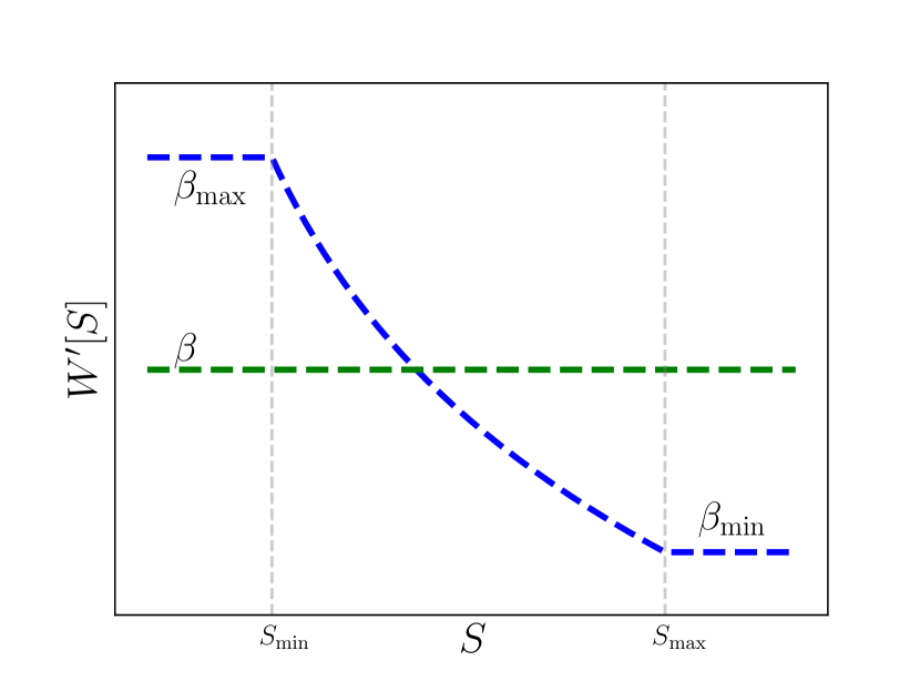
Figure 1: A cartoon of the Monte-Carlo sampling of $W[S]$. The green line represents a $W$ choice which will sample one $\beta$ value, while the blue line will sample all $\beta$ values between $\beta_{\mathrm{max}}$ and $\beta_{\mathrm{min}}$.

In a given Monte-Carlo simulation, we intend to sample a range of temperatures continuously over a prespecified range in pure glue QCD regularized on a finite space-time lattice. We will accomplish this using a reweighting method very similar to the old proposal of Berg and Neuhaus Berg and Neuhaus (1991). In this section we first show how a reweighted Monte-Carlo can be used to determine the susceptibility; then we show how the reweighted Monte-Carlo can be carried out; and finally we show how to determine the reweighting function itself. In practice, the numerical work proceeds in exactly the opposite order.

III.1 Susceptibility using reweighting

In the standard Monte-Carlo simulation one evaluates the partition function $\mathcal{Z}(\beta)$ shown below at a particular gauge coupling $\beta$ by generating gauge configurations with the probability distribution $\mathrm{d}P[U]$ as

$$\mathcal{Z}(\beta)=\int\mathcal{D}U\;e^{-\beta S},\quad\mathrm{d}P[U]=\frac{\mathrm{d}U\;e^{-\beta S}}{\mathcal{Z}(\beta)}.$$ (7)

Such a Monte-Carlo simulates a single temperature which is controlled by the gauge coupling $\beta$ since the lattice dimensions are fixed. In order to simulate a range of $\beta$ values and therefore a range of temperatures, the sampling weight in the usual Monte-Carlo in Eq. (7) is replaced with

$$\int\mathcal{D}U\;e^{-\beta S}\longrightarrow\int\mathcal{D}U\;e^{-W[S]}.$$ (8)

The weight function $W[S]$ is a general function of the action $S$, and its derivative can be interpreted, approximately, as the gauge coupling $\beta$ to use at a given action value:

$$W^{\prime}[S]\equiv\frac{\mbox{d}W[S]}{\mbox{d}S}=\beta[S].$$ (9)

In this sense, the usual Monte-Carlo has simply $W[S]=\beta S$ with the constant slope simulating the fixed coupling. We show how to cover a range of temperatures schematically in Figure 1. To get a fixed temperature one picks $W^{\prime}[S]=\beta$ as indicated by the green line in the figure; to cover a range of temperatures, one instead uses the blue line in the figure, for which $W^{\prime}[S]$ varies from $\beta_{\mathrm{max}}$ to $\beta_{\mathrm{min}}$ as $S$ changes from $S_{\mathrm{min}}$ to $S_{\mathrm{max}}$; here $S_{\mathrm{min}}$ and $S_{\mathrm{max}}$ are the average values of $S$ in simulations with coupling strengths $\beta_{\mathrm{max}}$ and $\beta_{\mathrm{min}}$ respectively. For $S_{0}$ an action value between these limiting choices, $W^{\prime}[S_{0}]$ is chosen to be the $\beta$ value for which the expectation value of the action would be $S_{0}$. Outside the range of interest, the weight function $W[S]$ then simulates two different constant gauge couplings $\beta_{\mathrm{max}}$ and $\beta_{\mathrm{min}}$. With this choice of $W[S]$, a single Markov chain Monte-Carlo will sample the entire range of $S$ values between $S_{\mathrm{min}}$ and $S_{\mathrm{max}}$ rather uniformly. The function $W^{\prime}[S]$ is not known a priori; we will return to its determination shortly, but will first discuss how a simulation with such a weight function can be carried out and used.

Once $W[S]$ is known, a Monte-Carlo simulation with $W[S]$ generates an ensemble which can be reweighted to determine expectation values at a given $\beta$ value $\beta_{0}$ via

$$\mathcal{Z}(\beta_{0}) = \int\mathcal{D}Ue^{-W[S]}\;e^{+W[S]-\beta_{0}S}$$

$$\propto \sum_{i}e^{W[S_{i}]-\beta_{0}S_{i}}\,,$$

where $i$ indexes the sampled configurations. In practice this partition function is used to determine expectation values for operators via

$$\langle\mathcal{O}\rangle=\mathcal{Z}^{-1}\int\mathcal{D}Ue^{-\beta_{0}S}\mathcal{O}\simeq\frac{\sum_{i}e^{W[S_{i}]-\beta_{0}S_{i}}\mathcal{O}_{i}}{\sum_{i}e^{W[S_{i}]-\beta_{0}S_{i}}}\,.$$ (11)

By establishing two reweighting functions $W[S]$ and $W_{Q}[S]$ for the $Q=0$ and $|Q|=1$ ensembles respectively, we can generate multi-temperature ensembles, labeled by $i$ and $iQ$, which respectively sample the $Q=0$ and the $|Q|=1$ ensembles across temperatures. The ratio needed in Eq. (6) is then given by

$$\frac{\chi_{\mathrm{top}}(\beta_{\mathrm{h}})a^{4}(\beta_{\mathrm{h}})}{\chi_{\mathrm{top}}(\beta_{\mathrm{c}})a^{4}(\beta_{\mathrm{c}})}$$ (12)

$$= \mathopen{}\mathclose{{}\left(\frac{\mathopen{}\mathclose{{}\left(\sum_{iQ}e^{W_{Q}[S_{iQ}]}e^{-\beta_{\mathrm{h}}S_{iQ}}}\right)\mathopen{}\mathclose{{}\left(\sum_{i\vphantom{Q}}e^{W[S_{i}]}e^{-\beta_{\mathrm{c}}S_{i}}}\right)}{\mathopen{}\mathclose{{}\left(\sum_{iQ}e^{W_{Q}[S_{iQ}]}e^{-\beta_{\mathrm{c}}S_{iQ}}}\right)\mathopen{}\mathclose{{}\left(\sum_{i\vphantom{Q}}e^{W[S_{i}]}e^{-\beta_{\mathrm{h}}S_{i}}}\right)}}\right)\,.$$

There are two subtleties associated with this expression. The first is that Eq. (III.1) only determines the partition function up to an overall multiplicative factor. However, this multiplicative factor cancels between the numerator and denominator expressions computed from the same sample. The second subtlety is that the partition function $\mathcal{Z}$ also has severe lattice-spacing dependent renormalizations, which we cannot easily compute. Fortunately, these cancel because each lattice spacing occurs once in the numerator and once in the denominator in Eq. (12).

III.2 Update algorithm with $W[S]$

In this section we explain the algorithm to perform a Monte-Carlo simulation with weight function $e^{-W[S]}$. Our aim is to generate a sampling with probability distribution

$$\mbox{d}P[U]=\frac{e^{-W[S[U]]}}{\int\mathcal{D}Ue^{-W[S[U]]}}$$ (13)

where $S[U]$ is the standard lattice gauge action and we assume that $W[S[U]]$ is a known differentiable function of the action $S$. Simulating such a weight requires a slight modification of the standard Hybrid Monte-Carlo (HMC) algorithm Duane et al. (1987).

As in the standard HMC algorithm, we introduce canonical momenta $\pi_{\mu}$ for the link variables $U_{\mu}$, and define a Hamiltonian for this system as

$$\mathcal{H}\big{(}\pi,U\big{)} \equiv \sum_{\mu,x}\frac{1}{2}(\pi_{\mu}(x))^{2}+W[S_{U}]$$ (14)

$$S_{U} = \sum_{\begin{picture}(4.0,4.0)\put(0.0,0.0){\line(1,0){4.0}}\put(0.0,4.0){\line(1,0){4.0}} \put(0.0,0.0){\line(0,1){4.0}}\put(4.0,0.0){\line(0,1){4.0}}\end{picture}}\mathopen{}\mathclose{{}\left(1-\frac{1}{3}\mathrm{Tr}\>\begin{picture}(6.0,6.0)\put(0.0,0.0){\line(1,0){6.0}}\put(0.0,6.0){\line(1,0){6.0}} \put(0.0,0.0){\line(0,1){6.0}}\put(6.0,0.0){\line(0,1){6.0}}\end{picture}}\right)$$ (15)

where $S_{U}$ in Eq. (15) is the standard Wilson gauge action written without the gauge coupling $\beta$ prefactor. The standard HMC would use the same Hamiltonian but with $W[S_{U}]$ replaced by $\beta S_{U}$, that is, it would use a strictly linear function for $W[S_{U}]$.

A single HMC update trajectory consists of the standard steps:

1. Picking a random canonical momentum $\pi_{\mu}(x)$ from a Gaußian ensemble independently for each of the elements of the Lie algebra.

2. Solving the following Hamilton equations of motion (shown here schematically):

   $$\frac{\mathrm{d}U}{\mathrm{d}t} =-i\pi U\,,$$ (16)

   $$\frac{\mathrm{d}\pi}{\mathrm{d}t} =iU^{\dagger}\frac{\partial W[S_{U}]}{\partial U}=iU^{\dagger}\frac{\mathrm{d}W[S_{U}]}{\mathrm{d}S_{U}}\frac{\partial S_{U}}{\partial U}$$ (17)

   for a total time $t_{0}$. The derivative with respect to $U_{\mu}$ is a Lie derivative and in this sense these equations are schematic representation. Here the time $t$ is a fictitious variable under which the Hamiltonian $\mathcal{H}$ is conserved.

   These Hamiltonian equations are discretized using a time-symmetric solver such as the leapfrog or Omelyan algorithms. Under these algorithms, one iteratively solves Eq. (16) for all link variables $U$ at fixed $\pi$, and then solves Eq. (17) for all $\pi$ variables at fixed $U$. Before applying Eq. (17), we must compute $S_{U}$ and use the (instantaneous) value of $W^{\prime}[S_{U}]$ in place of the usual factor of $\beta$ at each time step during the update.

   The use of a time-symmetric algorithm is essential, since it ensures the property that, if the pair $(U_{\mathrm{i}},\pi_{\mathrm{i}})$ (i for initial) is carried to $(U_{\mathrm{f}},\pi_{\mathrm{f}})$ under the update algorithm, then the pair $(U_{\mathrm{f}},-\pi_{\mathrm{f}})$ is carried to $(U_{\mathrm{i}},-\pi_{\mathrm{i}})$ up to roundoff error effects. This is sufficient to ensure that the algorithm converges, in a Fokker-Planck sense, to the probability distribution $\exp[-\mathcal{H}]$ provided that we also include a Metropolis accept/reject step.

3. In adding the Metropolis step, the change in the Hamiltonian $\Delta\mathcal{H}=\mathcal{H}(U_{\mathrm{f}},P_{\mathrm{f}})-\mathcal{H}(U_{\mathrm{i}},P_{\mathrm{i}})$ is compared to a random number drawn uniformly from the interval $[0,1]$: $\mathcal{R}[0,1]$. Whenever $e^{\Delta\mathcal{H}}<\mathcal{R}[0,1]$, we accept the change, and proceed with $U_{\mathrm{f}}$ as our new configuration. Otherwise we revert to $U_{\mathrm{i}}$, that is, we reject the update.

The only differences with respect to the standard HMC algorithm Duane et al. (1987) are the use of $W^{\prime}[S_{U}]$ the “instantaneous $\beta$ value” in place of $\beta$ in Eq. (17) and the use of $W[S_{U}]$ in place of $\beta S_{U}$ in the Metropolis accept-reject step. Both modifications are compatible with the time-symmetry of the update algorithm and therefore preserve detailed balance. With these modifications, the HMC algorithm now generates the desired probability distribution.

For the case of a $Q=1$ simulation, an additional accept-reject step is needed, in which we check to see whether the configuration has fallen down into the $Q=0$ sector and reject the update if this is the case. In practice we can buffer every $N$’th configuration and only perform this step after every $N$ HMC update steps, reverting to the last buffered configuration when the check fails. We define $Q$ as the lattice sum of an $a^{2}$-improved topological density definition after $\tau_{\mathrm{F}}=2.4a^{2}$ units of Wilson flow, as in Jahn et al. (2020). We find that values of $N=5$ or $N=10$ are adequate to preserve a good acceptance rate.

Lastly we remark on the optimal length of the individual trajectories. The figure of merit for trajectory length is the mean-squared change in $S_{U}$ per unit numerical effort. The numerical effort is approximately linear in trajectory length $t_{0}$. For a short trajectory, $\Delta S_{U}$ is linear, and $(\Delta S_{U})^{2}$ quadratic, in trajectory length; but beyond a certain (fairly short) trajectory length the action change saturates. Therefore we started with a study of how $(\Delta S_{U})^{2}$ varies with trajectory length and chose the value which maximizes $(\Delta S_{U})^{2}/t_{0}$; $t_{0}\simeq 0.75a$. A single trajectory leads to a change of $(\Delta S_{U}/S_{U})^{2}\simeq 3/N_{\mathrm{dof}}$ where $N_{\mathrm{dof}}=24V_{L}$ is the number of lattice degrees of freedom (3 polarizations and 8 colors per site). Therefore, for a well-chosen $W[S_{U}]$ function, since changes to $S_{U}$ accumulate in a Brownian fashion, the number of updates needed to explore the full $\beta$ range is of order

$$N_{\mathrm{updates}}\sim N_{\mathrm{dof}}\,\ln^{2}(\beta_{\mathrm{max}}/\beta_{\mathrm{min}}).$$ (18)

III.3 Choice and determination of $W[S]$

Now we return to the question of how to determine the weight function $W[S]$. We start by choosing the range of $\beta$ values we want to explore, $\beta\in[\beta_{\mathrm{min}},\beta_{\mathrm{max}}]$. A short fixed-$\beta$ Markov chain establishes $S_{\mathrm{max}}=\langle S_{U}\rangle_{\beta_{\mathrm{min}}}$ and $S_{\mathrm{min}}=\langle S_{U}\rangle_{\beta_{\mathrm{max}}}$. We then follow our procedure in Jahn et al. (2019, 2020) and choose a discrete set of values $S_{i},i=(0,\ldots N_{i})$ with $S_{0}=S_{\mathrm{min}}$ and $S_{N_{i}}=S_{\mathrm{max}}$; $W[S_{U}]$ will be determined by its values $W[S_{i}]$. However, because the update described above works best when both $W[S_{U}]$ and $W^{\prime}[S_{U}]$ are continuous functions, we shall interpolate $W[S_{U}]$ between these points using a cubic spline function, rather than using a piecewise linear function as in our previous papers. We extend $W[S]$ above $S_{\mathrm{max}}$ by choosing $W^{\prime}[S>S_{\mathrm{max}}]=\beta_{\mathrm{min}}$ and similarly we set $W^{\prime}[S<S_{\mathrm{min}}]=\beta_{\mathrm{max}}$; these are also the values of the first derivatives used in completing the definition of the spline function.

We will use the same automated improvement scheme to determine $W[S_{i}]$ as we introduced in Ref. Jahn et al. (2019) (see also Laine and Rummukainen (1998)). We generate a Markov chain using the update approach of the previous subsection, but after each update, we adjust the function $W[S_{U}]$ so as to make the current $S$ value less likely (implying that the current $S$ is oversampled). This is done by

1. determining $S_{i},S_{i+1}$ such that the current $S$ value lies between them, $S_{i}<S_{U}<S_{i+1}$

2. increasing $W[S_{i}]$ and $W[S_{i+1}]$ by $\Delta W[S_{i}]=\frac{s_{r}(S_{i+1}-S_{U})}{(S_{i+1}-S_{i})}$ and $\Delta W[S_{i+1}]=\frac{s_{r}(S_{U}-S_{i})}{(S_{i+1}-S_{i})}$. Here $s_{r}$ is an update strength which we explain next.

3. If $S_{U}$ is out of range, $W[S]$ is not updated.

4. If $i=0$ or $i+1=N_{i}$ so we are in the first or last interval, the boundary value is updated with double strength (since it is only updated half as often as other values).

The value $s_{r}$ is initially chosen so that, in the time it takes for the Monte-Carlo to go from the top to the bottom and back (see Eq. (18)), the $W[S_{i}]$ will change by of order 100. Each time the $S$-value makes its way from the first interval to the last and back (which we call a “sweep”), we reduce $s_{r}$; at first we reduce it by a factor of 2, but after the average $W[S_{i}]$ changes by less than 1 per sweep, we change it by a reduced amount. The update ends when five sweeps change the average $W[S_{i}]$ by a total of less than 1.

This approach is inefficient if the initial $W$ function is very far from its final form. Therefore we improve the initial guess from the simplest approach (that $W^{\prime}[S]$ is linear). Instead, we choose an intermediate $\beta$ value $\beta_{\mathrm{mid}}$ and perform a fixed-$\beta$ Monte-Carlo calculation to determine the associated $S_{\mathrm{mid}}$ value. We then fit $W^{\prime}$ to a quadratic, with values $(\beta_{\mathrm{max}},\beta_{\mathrm{mid}},\beta_{\mathrm{min}})$ at the points $(S_{\mathrm{min}},S_{\mathrm{mid}},S_{\mathrm{max}})$, integrate, and use this to determine starting guesses for the $W[S_{i}]$. With this approach, the initial and final $W$ functions differ by less than 100, as shown in Figure 2, which displays the difference between the initial and final $W$ function choice for the specific lattice and $\beta$ range described in the next section. The complete built $W^{\prime}$ is shown in Figure 3.

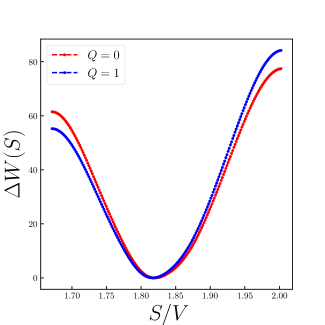
Figure 2: Difference between the final determined $W[S]$ and the initial guess.

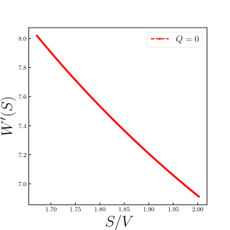
Figure 3: Final choice of $W^{\prime}[S]$ for the lattice study described in Section IV.

Finally, one must determine $W[S_{U}]$ for the $Q=1$ sector. Here we can take as an initial guess the $W[S_{U}]$ value determined in the $Q=0$ sector. To further refine this guess, we shift it by

$$W_{Q=1}[S]=W_{Q=0}[S]-11\ln(T/T_{0})$$ (19)

where $T$ is the temperature associated with the $\beta$ value described by the slope $W^{\prime}$ using a scale-setting relation between lattice coupling $\beta$ and temperature $T$, and $T_{0}$ is a reference temperature which could for instance be the temperature at $\beta_{\mathrm{min}}$. The factor 11 is the expected temperature dependence of $\chi_{\mathrm{top}}a^{4}$ when the lattice spacing $a$ varies as $1/T$, at leading perturbative order. Again, Eq. (19) is only used to refine the initial guess for $W_{Q=1}[S]$; we again perform an automated $W$-changing Markov chain to improve this guess; however the initial $s_{r}$ value can be made much smaller.

After the $W[S_{U}]$-setting Markov chains are completed, we freeze the values of $W_{Q=0,Q=1}[S]$ and use them in detailed-balance respecting Markov chains which we will use to determine the susceptibility as described in Subsection III.1.

IV Results

Table 1: Numerical cost of the simulation on a lattice four-volume $V=10\times 32^{2}\times 36$ with $\beta_{\mathrm{min}}=6.9076$ and $\beta_{\mathrm{max}}=8.01951$.

Procedure	$Q$	HMC Trajectories	Sweeps
Building	0	$4\times 10^{6}$	22
Building	1	$8\times 10^{6}$	17
Measurements	0	$6.8\times 10^{6}$	45
Measurements	1	$4.9\times 10^{6}$	35

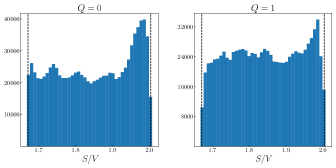
Figure 4: A histogram of the $S$ distribution of our Markov chain samples in the $Q=0$ sector (left) and the $Q=1$ sector (right).

In this section we present results of a simulation with aforementioned $W(S)$ sampling. Our goal is only to test the method; we will not study multiple lattice spacings to attempt a continuum limit. Instead, we choose one lattice geometry from among the geometries studied in Ref. Jahn et al. (2018, 2020), and which we can therefore use to compare our results for susceptibility ratios to those obtained via a competing technique. Our goal is to establish which approach, the one described here or the one described in Ref. Jahn et al. (2020), is more efficient at establishing the topological susceptibility at high temperature.

We choose to investigate a lattice with temporal extent $N_{\tau}=10$ and spatial extent $32^{2}\times 36$, with $(\beta_{\mathrm{min}},\beta_{\mathrm{max}})=(6.9076,8.01951)$, which corresponds, according to the scale setting calculation of Ref. Burnier et al. (2017) which we will use throughout, to $T_{\beta_{\mathrm{min}}}=2.5\,T_{\mathrm{c}}$ and $T_{\beta_{\mathrm{max}}}=9.4\,T_{\mathrm{c}}$. This scale-setting relation involves applying a fit to scale-setting data beyond the range where the reference has performed simulations, that is, an extrapolation, which means it may not be absolutely trustworthy. However, by expressing our results in terms of $\chi_{\mathrm{top}}(\beta)a^{4}(\beta)$, we can remain agnostic about the relation between $T$ and $\beta$ and just determine how accurately we can determine $\chi_{\mathrm{top}}a^{4}$ as a function of $\beta$ for this specific lattice geometry. Getting continuum results over a range of temperatures will then of course require multiple lattice $N_{\tau}$ values and a reliable scale setting. However, for the time being our goal is just to evaluate the precision-to-numerical-cost ratio of the technique, so we leave this problem for later. The number of updates used in each procedure are listed in Table 1. Note that an unfortunate choice of $s_{r}$ made the $Q=1$ building unnecessarily inefficient; a more careful choice should have required a fraction as many trajectories, so that the trajectory count would be dominated by the measurements.

We begin with a check that our $W[S]$ function correctly generates a rather uniform sample of configurations across the desired $\beta$ range. We investigate this by plotting a histogram of the $S$ values measured during the sampling Markov chain, both for the $Q=0$ and the $Q=1$ ensembles, shown in Figure 4. The sample is adequately uniform.

$T/T_{\mathrm{c}}$ $\beta$ $\ln(\chi_{\mathrm{top}}a^{4}(T)/\chi_{\mathrm{top}}a^{4}(2.8\,T_{\mathrm{c}}))$ 1-$\sigma$ stat. err 3.5  7.1771   -2.25 0.17 4.0 7.2885   -3.68 0.20 5.0 7.4764   -5.79 0.24 7.0 7.7629   -9.39 0.30 9.0 7.9788 -12.20 0.36

Table 2: Several temperatures, the corresponding $\beta$ values using the scale setting of Ref. Burnier et al. (2017), and our results for the log susceptibility ratio and its 1-sigma statistical error.

Our main results are presented in Figure 5, which shows how $\chi_{\mathrm{top}}a^{4}$ changes as a function of $\beta$ across the range we study, evaluated from our Markov chains using Eq. (12). We have chosen to use a value near the beginning of the $\beta$ range ($T=2.8\,T_{\mathrm{c}}$) as the low temperature and to express all other temperatures in relation to this one. The figure, and further data presented in Table 2, show that the error bars are smallest between nearby $\beta$ values and grow to around $\pm 0.35$ in $\ln(\chi_{\mathrm{top}})$ for the widest-separated temperatures. Our results agree within error bars of the results in Ref. Jahn et al. (2020) for those values where they are directly comparable.

V Discussion

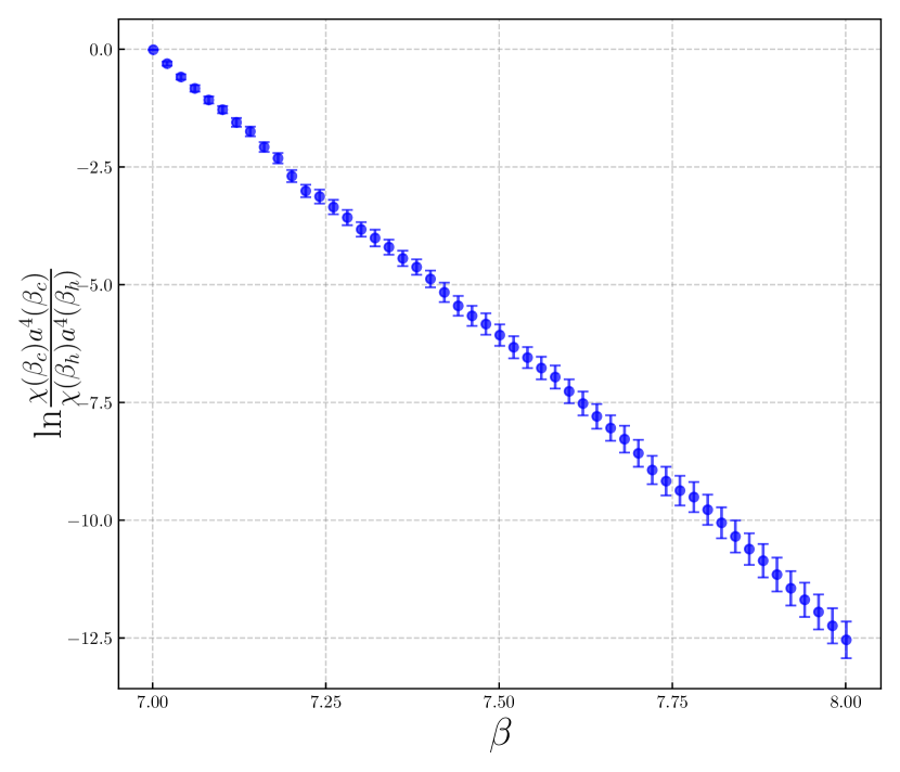
Figure 5: Results of the ratio in Eq. 12

We have shown that the method we propose can successfully find the $\beta$ dependence of $\chi_{\mathrm{top}}a^{4}$, and therefore the temperature dependence of the susceptibility if the line of constant physics (that is, $a(\beta)$) is known. This determines $\chi_{\mathrm{top}}$ over a range of temperatures if it is known at the lowest temperature, which is where it is most easily determined by other approaches.

There are two key questions. Is it more or less effective than the rather similar approach of Refs Borsanyi et al. (2016b); Frison et al. (2016)? And how does it compare with the approach of Ref. Jahn et al. (2020)?

The approach of Ref. Borsanyi et al. (2016b); Frison et al. (2016) computes $\mathrm{d}\ln(\chi_{\mathrm{top}}a^{4})/\mathrm{d}\beta$ at several $\beta$ values, which it integrates to determine $\chi_{\mathrm{top}}a^{4}(\beta)$. We review this approach and compare it to our own in an appendix. To summarize, in a high-statistics determination, the approaches have essentially the same numerical precision. However, if lower precision is desired, the numerical cost associated with building the $W(S)$ functions in our approach is essentially “dead weight” which does not contribute to the statistical power. The other approach does not suffer from this problem and so it is more efficient for a low-statistics determination. Our approach has the advantage that it automatically includes all intermediate temperatures, while the alternative bases the determined $\mathrm{d}\ln(\chi_{\mathrm{top}}a^{4})/\mathrm{d}\beta$ on a finite set of values which may leave discrete integration errors. But it is not difficult to use enough values to render this a minor concern.

Finally, we want to compare the numerical efficiency to the method of Ref. Jahn et al. (2020). Fortunately, the single lattice we investigated in this work was also used in that reference, and we can directly compare the error on $\chi_{\mathrm{top}}a^{4}(\beta_{\mathrm{h}})/\chi_{\mathrm{top}}a^{4}(\beta_{\mathrm{c}})$ found here with the error on the same quantity found there, along with the number of HMC trajectories needed in each case. In that reference $\chi_{\mathrm{top}}(T)$ was determined at $\beta=(6.90097,7.30916,7.76294)$, corresponding to $T=(2.5,4.1,7.0)\,T_{\mathrm{c}}$, a little narrower than the range considered here. The three determinations required a total of $9.2\times 10^{6}$ trajectories, about half the number which should have been needed here. The average trajectory length used was also shorter in that reference than what we used here. The the final errors on $\ln(\chi_{\mathrm{top}})$ in that study, for this lattice, were $(0.09,0.09,0.08)$ at the three temperatures. In comparison, in comparing $2.8\,T_{\mathrm{c}}$ to $7.0\,T_{\mathrm{c}}$ we find statistical errors of $0.30$. To reduce these errors to the level of the other study would therefore require about 10 times more statistics in our measurement runs, indicating that the present method is of order 10 times less numerically efficient. Moreover, Ref. Jahn et al. (2020) finds that the number of trajectories needed for a given statistical error barely changes as one increases the volume (larger aspect ratio) or makes the lattice finer (larger $N_{\tau}$ at fixed aspect ratio), whereas we know that the number of updates needed for the method described in this paper should scale with the number of lattice sites, see Eq. (18).

We conclude that our method is at least 10 times less efficient than the single-temperature reweighting approach of Jahn et al. (2020), and will become still less efficient as one goes closer to the large-volume and continuum limits. As we understand it, this also implies that it should be easier in principle to achieve small statistical errors with the approach of Jahn et al. (2020) than with the approach of Borsanyi et al. (2016b); Frison et al. (2016).

Appendix A Comparison with the slope method

Our approach is closely related to the approach of Refs. Borsanyi et al. (2016b); Frison et al. (2016), and as we understand it, the errors per numerical effort are nearly the same. To explain this conclusion, we start with a quick review of their approach, and then look at the issue of statistical power in each approach.

Their approach also seeks to compute Eq. (6) and then use a determination of $\chi_{\mathrm{top}}(\beta_{\mathrm{c}})$ to determine $\chi_{\mathrm{top}}$ at other temperatures. Taking the log of Eq. (6) we find

$$\ln\frac{\chi_{\mathrm{top}}(\beta_{\mathrm{h}})a^{4}(\beta_{\mathrm{h}})}{\chi_{\mathrm{top}}(\beta_{\mathrm{c}})a^{4}(\beta_{\mathrm{c}})} =\Big{(}\ln(Z_{1}(\beta_{\mathrm{h}}))-\ln(Z_{1}(\beta_{\mathrm{c}})\Big{)}$$

$$\phantom{=}{}-\Big{(}\ln(Z_{0}(\beta_{\mathrm{h}}))-\ln(Z_{0}(\beta_{\mathrm{c}})\Big{)}\,.$$ (20)

Now note that

$$Z(\beta) =\int\mathcal{D}A_{\mu}e^{-\beta S}\quad\Rightarrow$$

$$-\frac{\partial\ln Z}{\partial\ln\beta} =\frac{1}{Z}\int\mathcal{D}A_{\mu}e^{-\beta S}\beta S=\langle\beta S\rangle$$ (21)

the $\beta$ dependence of $\ln Z$ is set by the expectation value of the action. Therefore

$$\ln Z_{1}(\beta_{\mathrm{h}})-\ln Z_{1}(\beta_{\mathrm{c}})=-\int_{\ln\beta_{\mathrm{c}}}^{\ln\beta_{\mathrm{h}}}\langle\beta S\rangle_{1}\>\mathrm{d}(\ln\beta)$$ (22)

and the ratio we want is

$$\ln\frac{\chi_{\mathrm{top}}(\beta_{\mathrm{h}})a^{4}(\beta_{\mathrm{h}})}{\chi_{\mathrm{top}}(\beta_{\mathrm{c}})a^{4}(\beta_{\mathrm{c}})}=-\int_{\ln\beta_{\mathrm{c}}}^{\ln\beta_{\mathrm{h}}}\mathopen{}\mathclose{{}\left(\langle\beta S\rangle_{1}-\langle\beta S\rangle_{0}}\right)\mathrm{d}(\ln\beta)\,.$$ (23)

Refs. Borsanyi et al. (2016b); Frison et al. (2016) evaluate $\langle\beta S\rangle$ in both $Q=0$ and $Q=1$ ensembles at a number of $\beta$ values, which are then used to estimate this integral by, eg, the trapezoid rule.

To compute Eq. (23) using our approach, first write

$$\hskip 6.00006pt\int_{\ln\beta_{\mathrm{c}}}^{\ln\beta_{\mathrm{h}}}-\langle\beta S\rangle\;\mathrm{d}(\ln\beta)$$

$$=\int_{\ln\beta_{\mathrm{c}}}^{\ln\beta_{\mathrm{h}}}\frac{-\sum_{i}e^{W[S_{i}]-\beta S_{i}}\beta S_{i}}{\sum_{i}e^{W[S_{i}]-\beta S_{i}}}\mathrm{d}(\ln\beta)$$

$$=\int_{\ln\beta_{\mathrm{c}}}^{\ln\beta_{\mathrm{h}}}\frac{\mathrm{d}}{\mathrm{d}\ln\beta}\ln\mathopen{}\mathclose{{}\left(\sum_{i}e^{W[S_{i}]-\beta S_{i}}}\right)\mathrm{d}(\ln\beta)$$

$$=\ln\frac{\sum_{i}e^{W[S_{i}]-\beta_{\mathrm{h}}S_{i}}}{\sum_{i}e^{W[S_{i}]-\beta_{\mathrm{c}}S_{i}}}$$ (24)

so applying Eq. (11) to Eq. (23) leads directly to Eq. (12). Therefore the real difference between the approaches is whether Eq. (23) is estimated based on interpolating results for several temperatures, or using a single Markov chain which spans all temperatures.

Now consider the statistical power of each approach. The accuracy of a Monte-Carlo evaluation of $\langle\beta S\rangle$ is set by the variance of $\beta S$ and the number of independent configurations used. The variance should be reasonably approximated as that for $N_{\mathrm{dof}}$ Gaußian random variables: $\sigma_{\beta S}^{2}\simeq N_{\mathrm{dof}}/2$. Therefore order-1 errors in $\langle\beta S\rangle$ require $N_{\mathrm{dof}}/2$ evaluations. Since the expectation value determines an integrand, this is multiplied by the integration range, so $N_{\mathrm{dof}}/2$ evaluations return an error in the ratio of partition functions which is of order $\ln(\beta_{\mathrm{max}})-\ln(\beta_{\mathrm{min}})$. Evaluating $\langle\beta S\rangle$ at multiple $\beta$ values leads to a larger error at each evaluation, but because each is responsible for a narrower $\Delta\beta$ range and the errors are uncorrelated, the final statistical uncertainty is independent of the number of $\beta$ values used in the evaluation and depends only on the total number of Markov steps and the width of the $\beta$ range considered. The final error estimate is $\Delta\ln\chi=\ln(\beta_{\mathrm{max}}/\beta_{\mathrm{min}})\,\sqrt{N_{\mathrm{dof}}/2N_{\mathrm{updates}}}$. The error rises by $\sqrt{2}$ and $N_{\mathrm{updates}}$ is doubled when we recall that separate simulations are needed in the $Q=0$ and $Q=1$ sectors.

In comparison, we see in Eq. (18) that our approach can explore the full $\beta$ range, leading to order-1 errors in $\ln\chi$, in $N_{\mathrm{updates}}\sim N_{\mathrm{dof}}\,\ln^{2}(\beta_{\mathrm{max}}/\beta_{\mathrm{min}})$. Therefore the two approaches produce errors per unit numerical effort which are the same up to an order-1 factor. In a numerical experiment on a toy problem ($N$ independent Gaußian random variables $x$ with action $S=\sum x^{2}/2$) we find that the order-1 factor is in fact 1, so the two approaches have the same statistical power per compute time, provided that $W[S]$ is well determined and neglecting the computational effort expended in evaluating it.

We should also remark on how each approach is extended to full (unquenched) QCD. In each case the main challenge is dealing with the way quark masses must be varied with the lattice spacing and therefore with $\beta$: $m=m(\beta)$ (which must also be determined as part of the scale setting). This added $\beta$ dependence changes Eq. (A), replacing $\langle\beta S\rangle\to\langle\beta S+\beta\,\mathrm{d}m/\mathrm{d}\beta\,\bar{\psi}\psi\rangle$. In our approach one must replace $W[S]\to W[S]+\bar{\psi}(\not{D}+m(W^{\prime}[S]))\psi$ where we use $W^{\prime}$ in place of $\beta$ for the scale dependence of $m$. This amends Eq. (17) by the addition of the standard fermionic force term and by the replacement $\mathrm{d}W/\mathrm{d}S_{U}\to(\mathrm{d}W/\mathrm{d}S_{U})+(\mathrm{d}m/\mathrm{d}\beta)(\mathrm{d}W^{\prime}/\mathrm{d}S_{U})\langle\bar{\psi}\psi\rangle$ where $\langle\bar{\psi}\psi\rangle$ is the sum of the $\bar{\psi}\psi$ value over all sites in the current configuration. Finally, in Eq. (12), the $W-\beta S$ reweighting must be complemented by a determinant-ratio from the $S$-dependent mass to the physical mass for the desired $\beta$ value.

References

- Peccei and Quinn (1977) R. D. Peccei and H. R. Quinn, Phys. Rev. Lett. 38, 1440 (1977).
- Weinberg (1978) S. Weinberg, Phys. Rev. Lett. 40, 223 (1978).
- Wilczek (1978) F. Wilczek, Phys. Rev. Lett. 40, 279 (1978).
- Abbott and Sikivie (1983) L. F. Abbott and P. Sikivie, Phys. Lett. B120, 133 (1983).
- Preskill et al. (1983) J. Preskill, M. B. Wise, and F. Wilczek, Phys. Lett. B 120, 127 (1983).
- Irastorza and Redondo (2018) I. G. Irastorza and J. Redondo, Prog. Part. Nucl. Phys. 102, 89 (2018).
- Grilli di Cortona et al. (2016) G. Grilli di Cortona, E. Hardy, J. P. Vega, and G. Villadoro, JHEP 01, 034 (2016).
- Gorghetto and Villadoro (2019) M. Gorghetto and G. Villadoro, JHEP 03, 033 (2019), arXiv:1812.01008 [hep-ph] .
- Moore (2018) G. D. Moore, Proceedings, 35th International Symposium on Lattice Field Theory (Lattice 2017): Granada, Spain, June 18-24, 2017, EPJ Web Conf. 175, 01009 (2018).
- Borsanyi et al. (2016a) S. Borsanyi, M. Dierigl, Z. Fodor, S. D. Katz, S. W. Mages, D. Nogradi, J. Redondo, A. Ringwald, and K. K. Szabo, Phys. Lett. B 752, 175 (2016a).
- Borsanyi et al. (2016b) S. Borsanyi et al., Nature 539, 69 (2016b).
- Frison et al. (2016) J. Frison, R. Kitano, H. Matsufuru, S. Mori, and N. Yamada, JHEP 09, 021 (2016).
- Bonati et al. (2018) C. Bonati, M. D’Elia, G. Martinelli, F. Negro, F. Sanfilippo, and A. Todaro, JHEP 11, 170 (2018), [JHEP18,170(2020)], arXiv:1807.07954 [hep-lat] .
- Jahn et al. (2018) P. T. Jahn, G. D. Moore, and D. Robaina, Phys. Rev. D98, 054512 (2018), arXiv:1806.01162 [hep-lat] .
- Jahn et al. (2020) P. T. Jahn, G. D. Moore, and D. Robaina, (2020), arXiv:2002.01153 [hep-lat] .
- Laio et al. (2016) A. Laio, G. Martinelli, and F. Sanfilippo, JHEP 07, 089 (2016).
- Wang and Landau (2001) F. Wang and D. P. Landau, Phys. Rev. Lett. 86, 2050 (2001).
- Berg and Neuhaus (1991) B. A. Berg and T. Neuhaus, Phys. Lett. B267, 249 (1991).
- Duane et al. (1987) S. Duane, A. D. Kennedy, B. J. Pendleton, and D. Roweth, Phys. Lett. B 195, 216 (1987).
- Jahn et al. (2019) P. T. Jahn, G. D. Moore, and D. Robaina, Eur. Phys. J. C79, 510 (2019), arXiv:1805.11511 [hep-lat] .
- Laine and Rummukainen (1998) M. Laine and K. Rummukainen, Nucl. Phys. B535, 423 (1998).
- Burnier et al. (2017) Y. Burnier, H. T. Ding, O. Kaczmarek, A. L. Kruse, M. Laine, H. Ohno, and H. Sandmeyer, JHEP 11, 206 (2017), arXiv:1709.07612 [hep-lat] .
- (23) http://luscher.web.cern.ch/luscher/openQCD/index.html.