Weakly bound $H$ dibaryon from SU(3)-flavor-symmetric QCD

Abstract

We present the first study of baryon-baryon interactions in the continuum limit of lattice QCD, finding unexpectedly large lattice artifacts. Specifically, we determine the binding energy of the $H$ dibaryon at a single quark-mass point. The calculation is performed at six values of the lattice spacing $a$, using O($a$)-improved Wilson fermions at the SU(3)-symmetric point with $m_{\pi}=m_{K}\approx 420$ MeV. Energy levels are extracted by applying a variational method to correlation matrices of bilocal two-baryon interpolating operators computed using the distillation technique. Our analysis employs Lüscher’s finite-volume quantization condition to determine the scattering phase shifts from the spectrum and vice versa, both above and below the two-baryon threshold. We perform global fits to the lattice spectra using parametrizations of the phase shift, supplemented by terms describing discretization effects, then extrapolate the lattice spacing to zero. The phase shift and the binding energy determined from it are found to be strongly affected by lattice artifacts. Our estimate of the binding energy in the continuum limit of three-flavor QCD is $B_{H}^{\text{SU(3)${}_{\rm f}$}}=4.56\pm 1.13_{\rm stat}\pm 0.63_{\rm syst}$ MeV.

The $H$ dibaryon is a scalar six-quark state with flavor content $uuddss$, originally proposed in 1977 by Jaffe Jaffe (1977). Despite years of effort, experimental searches have not produced any hard evidence for its existence Takahashi et al. (2001); Ahn et al. (2013); Kim et al. (2013). However, an upper bound on its binding energy has been derived from the observed production and decay pattern of a doubly strange $\isotope[6][\Lambda\Lambda]{He}$ hypernucleus Takahashi et al. (2001); Ahn et al. (2013).

Studying the properties of a potential $\Lambda$-$\Lambda$ bound state will help our understanding of the hadronic ($\Lambda$-$\Lambda$) interaction, which is relevant for the physics of double hypernuclei, neutron-rich matter and neutron stars. Recently, experimental data for two-particle correlations in p-p, p-Pb and Au-Au collisions Adamczyk et al. (2015); Acharya et al. (2019a, b) have been analyzed to constrain the $\Lambda$-$\Lambda$ interaction and provide model estimates for the binding energy of the $H$ dibaryon. In addition, a dedicated experiment is planned to search for it at J-PARC Ichikawa et al. (2021). Other approaches to study the $H$ dibaryon include chiral effective field theory Haidenbauer and Meißner (2011); Haidenbauer et al. (2016); Li et al. (2018); Baru et al. (2019) and lattice QCD.

Lattice QCD studies of dibaryons and baryon-baryon scattering are very challenging because of the signal-to-noise problem Parisi (1984); Lepage (1989) and the complexity of contractions. In response to an inconsistency between results in the nucleon-nucleon sector Iritani et al. (2017); Wagman et al. (2017), there has been a recent focus on improved baryon-baryon spectroscopy methods Francis et al. (2019); Hörz et al. (2021); Amarasinghe et al. (2021). This work goes beyond that to achieve control over all systematic effects for the $H$-dibaryon channel at one unphysical quark mass point.

There is a long history of calculations studying whether the $H$ dibaryon is a prediction of QCD Mackenzie and Thacker (1985); Iwasaki et al. (1988); Pochinsky et al. (1999); Wetzorke et al. (2000); Wetzorke and Karsch (2003); Luo et al. (2007, 2011); Beane et al. (2011a, b, 2012, 2013); Inoue et al. (2010, 2011, 2012); Francis et al. (2019); Sasaki et al. (2020). Results for the binding energy $B_{H}$ from these calculations vary considerably, with estimates ranging from a few MeV up to 75 MeV, depending on the methodology and/or the value of the pion mass (see Fig. 5). Recently, employing near-physical pion and kaon masses, the HAL QCD Collaboration reported that the $\Lambda$-$\Lambda$ interaction is only weakly attractive and does not sustain a bound or resonant dihyperon Sasaki et al. (2020).

In our previous work Francis et al. (2019), using gauge fields with dynamical $u$ and $d$ quarks and a quenched $s$ quark, we found that the distillation method Peardon et al. (2009) produced a better determination of the two-baryon spectrum than previously used methods. At a heavy SU(3)-symmetric point with a pion mass of 960 MeV, we obtained $B_{H}=19\pm 10$ MeV.

In this letter we extend our calculations to lattice QCD with dynamical $u$, $d$, and $s$ quarks with degenerate masses set to their physical average value, corresponding to $m_{\pi}=m_{K}\approx 420$ MeV . We present the first systematic study of discretization effects in a multibaryon system, by computing finite-volume spectra at several lattice spacings, extrapolating the corresponding scattering phase shift to the continuum limit, and determining the binding energy. As shown in Fig. 1, at vanishing lattice spacing, we find $B_{H}^{\text{SU(3)${}_{\rm f}$}}=4.56\pm 1.30$ MeV, which is smaller than the result at the coarsest lattice spacing by a factor of about 7.5. We conclude that a thorough investigation of lattice artifacts is indispensable for answering the question whether a bound $H$ dibaryon exists in nature.

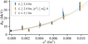
Figure 1: Binding energy versus squared lattice spacing, from fits to the full $p^{2}$ range (blue squares and solid curves) and to the near-threshold region (orange circles and dashed curves). Points are from fits to individual ensembles and curves are from the combined fits to the spectra of different subsets of the ensembles; they are not fitted to these points. Gray diamonds show results from the small-volume ensembles and the black cross shows our final estimate.

Our calculations are based on a set of eight gauge ensembles generated by CLS Bruno et al. (2015), with a nonperturbatively O($a$)-improved Wilson-clover fermion action. These ensembles have six different values of the lattice spacing and multiple box sizes $L$ (all satisfying $m_{\pi}L\geq 4.4$) as shown in the inset of Fig. 3 sup .

For each ensemble, we determine the energy levels in the rest frame and in four moving frames. To this end, in each frame we compute a Hermitian matrix of two-point correlation functions from a basis of interpolating operators: $C_{ij}(t)\equiv\langle\mathcal{O}_{i}(t)\mathcal{O}_{j}^{\dagger}(0)\rangle$. The finite-volume spectrum $\{E_{n}\}$ determines the exponential fall-off of $C_{ij}(t)$.

The building blocks of our operator basis are products of two single-baryon operators projected to momenta $\vec{p}_{1}$ and $\vec{p}_{2}$ with total spin zero or one. For each frame momentum $\vec{P}=\vec{p}_{1}+\vec{p}_{2}$, we take linear combinations that transform under the trivial irreducible representation of the little group of $\vec{P}$, which contains the ${}^{1}S_{0}$ scattering channel sup . Following Refs. Inoue et al. (2010); de Swart (1963), the flavor content of our interpolating operators is a linear combination of isospin-zero $\Lambda\Lambda$, $\Sigma\Sigma$, and symmetric $N\Xi$ that corresponds to the singlet irreducible representation of SU(3)-flavor.

Calculating the correlation functions of bilocal operators requires the ability to compute “timeslice-to-all” quark propagators. As in our previous study Francis et al. (2019), we have used the distillation technique Peardon et al. (2009); sup .

The finite-volume energy levels in each frame are determined by solving a generalized eigenvalue problem (GEVP) Lüscher and Wolff (1990); Blossier et al. (2009); sup , $C(\tau_{D})v_{n}=\lambda_{n}C(\tau_{0})v_{n}$, for fixed $\tau_{0}$ and $\tau_{D}$ satisfying $\tau_{D}>\tau_{0}\geq\tau_{D}/2$. We then use the eigenvectors $v_{n}$ to construct $\tilde{C}_{nm}(t)\equiv v_{n}^{\dagger}C(t)v_{m}$, an approximately diagonalized correlator matrix. We have verified that different combinations of $(\tau_{0},\tau_{D})$ yield consistent results across a wide range of values sup .

Before fitting to the data, we divide the rotated two-baryon correlators by a product of two single-baryon correlators that form the corresponding two-baryon noninteracting level $R_{n}(t)\equiv\tilde{C}_{nn}(t)/[C_{\Lambda}^{\vec{p}_{1}}(t)C_{\Lambda}^{\vec{p}_{2}}(t)]$, where $C_{\Lambda}^{\vec{p}_{i}}$ is a single-$\Lambda$ correlator with momentum $\vec{p}_{i}$, and the total frame momentum is $\vec{p}_{1}+\vec{p}_{2}$. The leading term in this ratio falls off exponentially with the shift $\Delta E$ of the interacting two-baryon energy away from the noninteracting level. In the ratio, we observe a partial cancellation of correlated statistical fluctuations and residual contributions from excited states, which helps in the reliable determination of $\Delta E$.

Our finite-volume energies are determined from single-exponential fits to $R_{n}(t)$. For all levels, we choose $t_{\rm min}$, i.e. the smallest time separation included in the fits, to lie in the plateau region of $R_{n}(t)$. We also aim to have $t_{\rm min}$ lie in the plateau region of the single-baryon correlators, and in the majority of cases we set it to be the first time separation in this plateau region. Since the single-baryon correlators take longer than the two-baryon correlators to reach their asymptotic behavior, this ensures that all correlators entering the ratio have little to no excited-state contamination. In some cases, however, the signal of $R_{n}(t)$ is already significantly degraded at the start of the single-baryon plateau region, and we are led to choose a slightly lower $t_{\rm min}$ that still lies within the plateau region of the correlator ratio. For all levels, we estimate the sensitivity to $t_{\rm min}$ by extracting an alternative spectrum with $t_{\rm min}$ further lowered, and use it in subsequent analyses to estimate the systematic uncertainty of our energy determination.

The fits also yield the couplings between each energy eigenstate and our operators. For each frame that includes a spin-one operator, we find one eigenstate that has strong overlap with only that operator, allowing for a simple identification of the spin-one dominated states.

Figure 2 shows the effective energy difference $\Delta E_{\rm eff}(t)\equiv-\frac{d}{dt}\log R(t)$ and the extracted $\Delta E$ for the ground state in frame $(0,0,1)$ on four ensembles that differ primarily in their lattice spacing. This level is particularly important because it is the closest to the bound-state pole determined in the phase shift analysis. An overview of the finite-volume spectrum is shown in Fig. 3, where the energy shifts are transformed to the center-of-mass momentum $p$. For every level, these two figures show a clear increasing trend as the lattice spacing is reduced, indicating that discretization effects are significant.

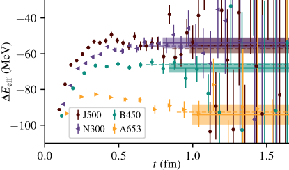
Figure 2: Effective energy difference obtained from $R_{0}(t)$ for the ground state in frame $(0,0,1)$ on four ensembles with similar volumes. The bands show $\Delta E$ determined from a single-exponential fit to $R_{0}(t)$ and also indicate the range of $t$ used for the fit. The dashed lines show the alternative fit used to estimate systematic uncertainty.

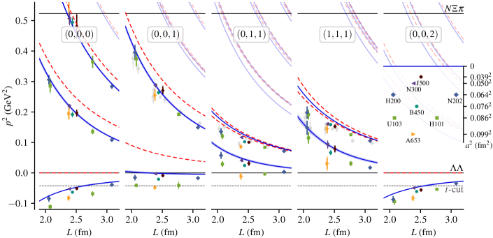
Figure 3: Finite-volume spectrum: center-of-mass scattering momentum $p^{2}$ versus lattice extent $L$. The five different frames are shown separately and are labelled with $\vec{D}\equiv\vec{P}L/(2\pi)$. Colored points show spin-zero levels and gray points (offset horizontally) show levels identified as spin one. Solid horizontal lines show the two- and three-particle thresholds while dashed horizontal lines represent the $t$-channel cut. The noninteracting spectrum is denoted by red dashed curves, and solid blue curves show the interacting spectrum determined in the continuum (see main text); the pale curves correspond to levels that have not been determined in the lattice calculation. The inset serves as a legend, showing $L$ and $a^{2}$ for the ensembles used in this work.

Given the two-particle scattering amplitude, Lüscher’s finite-volume quantization condition Lüscher (1991) and its generalizations Rummukainen and Gottlieb (1995); Briceño et al. (2013); Briceño (2014) determine the finite-volume spectrum, up to exponentially suppressed corrections, between the $t$-channel cut ($p^{2}>-m_{\pi}^{2}/4$) and the three-particle threshold ($E_{\text{cm}}<2m_{B}+m_{\pi}$). Since the quantization condition is diagonal in spin Briceño et al. (2013); Briceño (2014), the spin-one part of the scattering amplitude does not affect the spin-zero finite-volume spectrum, and we choose to ignore the spin-one states. In addition, we neglect higher partial waves starting from ${}^{1}D_{2}$. In this case, the quantization condition yields the ${}^{1}S_{0}$ phase shift $\delta(p)$ at the momentum corresponding to each finite-volume energy level:

$$p\cot\delta(p)=\frac{2}{\sqrt{\pi}L\gamma}Z_{00}^{\vec{P}L/(2\pi)}\left(1,\left(\frac{pL}{2\pi}\right)^{2}\right),$$ (1)

where $\gamma=E/E_{\text{cm}}$ and $Z_{00}^{\vec{D}}$ is a generalized zeta function. In addition to excluding levels with too-low or too-high $p^{2}$ from our analysis, we must also exclude the first excited levels in frames $(0,1,1)$ and $(1,1,1)$, as the ${}^{1}D_{2}$ partial wave is necessary to describe their position below the lowest noninteracting level sup .

The quantization conditions do not take discretization effects into account; strictly speaking, they are only valid in the continuum. There is no general formalism for finite-volume quantization at nonzero lattice spacing, except for a simple model studied in Ref. Körber et al. (2019). In principle, discretization effects would affect both the scattering amplitude and the finite-volume quantization condition. Effects on the former could include $a$-dependence and frame-dependence of the scattering amplitude, as well as couplings between $J^{P}$ that are forbidden in the continuum. Effects on the latter could include a modification of the zeta functions Körber et al. (2019). Either way, discretization effects might spoil the factorization that separates spin-zero from spin-one. Lacking a rigorous understanding, we have elected to model discretization effects in a simple way, by allowing the parameters of the phase shift to depend on $a$.

Our primary analysis is based on combined fits of the dependence of the phase shift on both $p^{2}$ and $a$. Specifically, our model is

$$p\cot\delta(p)=\sum_{i=0}^{N-1}c_{i}p^{2i},\quad c_{i}=c_{i0}+c_{i1}a^{2}.$$ (2)

Concerning the dependence on $p^{2}$, we fit in two ways. The first uses the near-threshold region, $|p^{2}|\lesssim m_{\pi}^{2}/4$ (where the effective range expansion converges), with $N=2$ terms for the dependence on $p^{2}$. The second uses the full $p^{2}$ range, starting from the $t$-channel cut and stopping just below the three-particle threshold, with $N=3$. Given $\{c_{ij}\}$, solving Eq. (1) yields a discrete spectrum of $p^{2}$ for each volume and frame; we fit these to the lattice spectra. For comparison, we also performed fits to individual ensembles, neglecting discretization effects. Given $\delta(p)$, a solution below threshold to $p\cot\delta(p)=-\sqrt{-p^{2}}$ corresponds to a bound state pole. All of the fits yielded a bound $H$ dibaryon.

Our preferred fit is to all ensembles using the full $p^{2}$ range; the corresponding continuum interacting energy levels are shown as blue curves in Fig. 3. In addition to the alternative spectrum fit range, we estimate the systematic uncertainty using the root-mean-square difference of alternative combined fits that cover all combinations of cuts on $p^{2}$ (full range or near threshold), $a$ (all six or the finest four), and $L$ (excluding $L\approx 2.1$ fm or not). All of these fits have acceptable fit quality, with $p$-values between 0.2 and 0.9. We explored adding an $a^{3}$ term in Eq. (2) but found that this reduces $\chi^{2}$ by at most 1.1 for each additional fit parameter, a sign of overfitting.

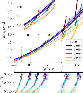
Figure 4: Upper panel: $p\cot\delta$ versus $p^{2}$, normalized using the pion mass, with inset showing the near-threshold region. Data are shown for the four ensembles with $L\approx 2.4$ fm. Curves show the result from a combined fit, at nonzero lattice spacing (indicated by color) and in the continuum (blue with error band); intersections with the red dashed curve correspond to bound-state poles. Only points to the right of the vertical dashed line are included in the fit. Lower panel: level-by-level cross check of continuum extrapolation, with adjustments on three ensembles to match the target volume $L^{*}$. Pale points (displaced vertically) show the levels before adjustment. The spectrum obtained from the continuum phase shift is indicated using blue crosses. Curves show continuum extrapolations of the form $b_{0}+b_{1}a^{2}$ excluding the coarsest lattice spacing (solid magenta) and $b_{0}+b_{1}a^{2}+b_{2}a^{3}$ using all four lattice spacings (dashed cyan).

The phase shifts from the preferred fit, in the continuum and at nonzero lattice spacing corresponding to the four ensembles with $L\approx 2.4$ fm (J500, N300, B450, A653), are shown in Fig. 4. Since these ensembles have similar values of $L$, they allow us to perform a cross check, shown in the lower panel. We select the volume of ensemble B450 as our target and call this box size $L^{*}$. For the three other lattice spacings, we estimate each energy level at $L^{*}$ by shifting from $L$ using the quantization condition: $p^{2}(L^{*})\approx p^{2}(L)+p^{2}_{\text{q.c.}}(L^{*})-p^{2}_{\text{q.c.}}(L)$. For each energy level, we then study the dependence of $p^{2}(L^{*})$ on the lattice spacing and compare it with the value obtained from applying the quantization condition to the continuum limit of the preferred fit. The cross check shows that a level-by-level continuum extrapolation at $L^{*}$ is consistent with the latter. However, some levels show curvature in the dependence on $a^{2}$ and the fixed-$L^{*}$ extrapolation is less precise, making it less useful than the combined fits.

Near threshold, we can write $p\cot\delta=-1/a_{0}+r_{0}p^{2}/2+O(p^{4})$, where $a_{0}$ is the scattering length and $r_{0}$ is the effective range. We obtain

$$a_{0}^{\text{SU(3)${}_{\rm f}$}} =3.30\pm 0.36\pm 0.21\text{ fm},$$ (3)

$$r_{0}^{\text{SU(3)${}_{\rm f}$}} =0.98\pm 0.04\pm 0.05\text{ fm},$$ (4)

where the first error is statistical and the second is systematic. The dependence of the $H$ dibaryon binding energy on $a$ is shown in Fig. 1; in the continuum, we obtain

$$B_{H}^{\text{SU(3)${}_{\rm f}$}}=4.56\pm 1.13\pm 0.63\text{ MeV},$$ (5)

which is substantially lower than the binding energies determined at nonzero lattice spacing, except on the finest two of our ensembles.

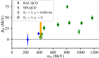
Figure 5: Binding energy versus pion mass: our results — three-flavor QCD in the continuum [diamond, Eq. (5)] and two-flavor QCD at nonzero lattice spacing (crosses sup ) — and published values Beane et al. (2011a, b, 2013); Inoue et al. (2011, 2012). Green and blue symbols refer to SU(3)-symmetric and broken cases, respectively. The orange vertical band represents the range of binding energies obtained at nonzero lattice spacing for $N_{f}=3$.

We have reported the first lattice study of a baryon-baryon system in the continuum limit. The crucial elements of our methodology are the finite-volume quantization condition, supplemented by terms describing discretization effects and applied over a wide range of lattice spacings, as well as the subsequent extrapolation to the continuum limit. We conclude that cutoff effects are large and cannot be ignored in an investigation of the $H$ dibaryon using lattice QCD; it will be essential to study their importance in other multibaryon systems such as the deuteron, where calculations disagree Iritani et al. (2017); Wagman et al. (2017); Hörz et al. (2021). Our final result for the binding energy, given in Eq. (5), suggests the existence of a weakly bound $H$ dibaryon, which is not only at variance with Jaffe’s original bag model prediction Jaffe (1977) of a deeply bound $uuddss$ state, but is also substantially lower than the binding energies determined in previous lattice calculations Beane et al. (2011a, b, 2012, 2013); Inoue et al. (2010, 2011, 2012); Francis et al. (2019) at nonzero lattice spacing (see Fig. 5). This adds to the evidence against deeply bound hexaquark dark matter Farrar (2017); Gross et al. (2018); Farrar (2018); Kolb and Turner (2019); McDermott et al. (2019); Lees et al. (2019); Azizi et al. (2020); Farrar et al. (2020). An obvious caveat is that our calculation was performed for one set of degenerate quark masses. The issue of SU(3) symmetry breaking — which is crucial, since the splitting between physical $\Lambda\Lambda$ and $N\Xi$ thresholds is larger than $B_{H}^{\text{SU(3)${}_{\rm f}$}}$ — is currently under investigation Padmanath et al. . Previous estimates based on extrapolations of lattice data found a bound state at the physical point unlikely Shanahan et al. (2011); Haidenbauer and Meißner (2011); Inoue et al. (2012); Yamaguchi and Hyodo (2016); Li et al. (2018); our smaller binding energy should make it even less likely.

In this supplement, we provide additional details for our calculation. Section I specifies the lattice action and ensembles. The precise definitions of our interpolating operators are given in Section II. Our implementation of the distillation approach is described in Section III. We provide further details about our determination of the spectrum in Section IV and our combined fits to the spectra at different lattice spacings in Section V. The analysis of two $N_{f}=2$ ensembles is provided in Section VI. Finally, Section VII describes the spectrum data being made available with this article.

I Lattice ensembles

Our calculations are based on a set of gauge ensembles with $N_{f}=2+1$ flavors of dynamical quarks, generated by CLS using the openQCD code suite Lüscher and Schaefer (2013) and listed in Table SI. The fields are described by the tree-level O($a^{2}$)-improved Lüscher-Weisz action and the O($a$)-improved Wilson-Clover action in the quark sector, with the improvement coefficient $c_{\rm sw}$ tuned to the nonperturbative determination of Ref. Bulava and Schaefer (2013). Open or periodic boundary conditions in the time direction are employed. All ensembles realize SU(3) symmetry, with $m_{\pi}=m_{K}\approx 420$ MeV, at six different values of the lattice spacing, covering a range between 0.04 and 0.1 fm. Here we also take the opportunity to extend our earlier calculations with $N_{f}=2$ flavors of dynamical quarks Francis et al. (2019). The respective simulation parameters are listed in Table SI, and a detailed description can be found in Section VI.

As discussed in Ref. Bruno et al. (2017), the quark masses are not exactly matched among the different lattice spacings. Given our choice of scale setting, this corresponds to a 3% variation in the pion mass, from 411 to 424 MeV. This is expected to produce a shift in the octet baryon mass of order 10 MeV, preventing a simple study of discretization effects in the octet baryon mass. However, the latter also varies by just 3% among our ensembles, which puts a likely upper bound on the size of discretization effects. For our main study of baryon-baryon interactions, we always determine energy differences from noninteracting levels and convert them to $p^{2}$ using the baryon mass determined on the same ensemble, cancelling the leading effect due to slightly varying baryon masses. Our expectation is that the mistuning of the pion mass will affect the energy differences at the few-percent level, which is much smaller than our statistical uncertainty.

Table SI: Overview of lattice ensembles. Each ensemble is characterized by the gauge coupling parameter $\beta$, the quark hopping parameter $\kappa$, the lattice size, and the temporal boundary condition. For $N_{f}=3$, the lattice spacing $a$ was determined for the second-finest lattice spacing from the result in Ref. Bruno et al. (2017) and scaled to the other lattice spacings using the gradient flow scale $t_{0}$ Lüscher (2010) determined at the symmetric point. For the ensembles with $N_{f}=2$ we use the lattice spacing determined in Ref. Fritzsch et al. (2012). The masses of the light octets of pseudoscalar mesons and spin-1/2 baryons are given by $m_{\pi}$ and $m_{B}$, respectively. On each of the $N_{\text{conf}}$ gauge configurations analyzed, $N_{\text{tsrc}}$ source timeslices were used. Including both forward and backward-propagating states, the total number of measurements used is $N_{\text{meas}}=N_{t}N_{\text{conf}}$, where $N_{t}=2(N_{\text{tsrc}}-N_{\text{skip}})$. To avoid boundary effects, we omit some potential measurements, such as the backward-propagating states from the first source timeslice; thus, $N_{\text{skip}}$ is 0 for the ensembles with periodic boundary conditions and between 1 and $N_{\text{tsrc}}/2$ for the ensembles with open boundary conditions. Finally, $N_{\text{LapH}}$ is the number of low modes of the Laplacian used in the Laplacian-Heaviside smearing.

Label	$N_{f}$	$\beta$	$\kappa$	size	bdy. cond.	$a$ (fm)	$m_{\pi}$ (MeV)	$L$ (fm)	$m_{\pi}L$	$m_{B}$ (GeV)	$N_{\text{conf}}$	$N_{\text{tsrc}}$	$N_{\text{meas}}$	$N_{\text{LapH}}$
J500	3	3.85	0.136852	$64^{3}\times 192$	open	0.0392	411	2.5	5.2	1.18	1341	12	24138	36
N300	3	3.70	0.137	$48^{3}\times 128$	open	0.0498	422	2.4	5.1	1.20	2047	12	24564	32
N202	3	3.55	0.137	$48^{3}\times 128$	open	0.0642	412	3.1	6.4	1.17	899	8	10788	68
H200	3	3.55	0.137	$32^{3}\times 96$	open	0.0642	419	2.1	4.4	1.20	2000	8	16000	20
B450	3	3.46	0.13689	$32^{3}\times 64$	periodic	0.0762	417	2.4	5.2	1.18	1612	8	25762	32
H101	3	3.40	0.13675962	$32^{3}\times 96$	open	0.0865	417	2.8	5.9	1.16	2016	4	12096	48
U103	3	3.40	0.13675962	$24^{3}\times 128$	open	0.0865	414	2.1	4.4	1.18	5658	5	45264	20
A653	3	3.34	0.1365716	$24^{3}\times 48$	periodic	0.0992	424	2.4	5.1	1.17	5050	4	40400	32
E5	2	5.30	0.13625	$32^{3}\times 64$	periodic	0.0658	437	2.1	4.7	1.29	2000	4	16000	30
E1	2	5.30	0.1355	$32^{3}\times 64$	periodic	0.0658	979	2.1	10.4	2.03	168	8	2688	30

II Interpolating operators

In our previous study Francis et al. (2019), we found that bilocal two-baryon operators are more effective than local hexaquark operators at identifying the low-lying spectrum; therefore, in this work we use only the former. To begin, we define the single-octet-baryon operators, which make use of the three-quark combination

$$[rst]_{\alpha}=\frac{1}{\sqrt{18}}\epsilon^{ijk}(s^{T}_{i}C\gamma_{5}P_{+}t_{j})r_{k\alpha}.$$ (S1)

Here $r$, $s$, and $t$ denote smeared quark fields of generic flavor at the same point and $P_{+}=(1+\gamma_{0})/2$ is a positive-parity projector. This satisfies $[rst]=-[rts]$ and $P_{+}([rst]+[str]+[trs])=0$. The members of the the SU(3)-flavor octet are defined following Ref. Inoue et al. (2010):

$$\begin{gathered}n=[dud],\quad p=[uud],\\ \Sigma^{-}=-[dds],\quad\Sigma^{0}=\tfrac{-1}{\sqrt{2}}([dus]+[uds]),\quad\Sigma^{+}=-[uus],\\ \Lambda=\tfrac{1}{\sqrt{6}}(2[sud]-[uds]-[dsu]),\\ \Xi^{-}=[ssd],\quad\Xi^{0}=[ssu].\end{gathered}$$ (S2)

The spin-zero and spin-one two-baryon operators are defined as follows:

$$[B_{1}B_{2}]_{0}(\vec{p}_{1},\vec{p}_{2}) =\sum_{\vec{x},\vec{y}}e^{-i\vec{p}_{1}\cdot\vec{x}}e^{-i\vec{p}_{2}\cdot\vec{y}}B_{1}^{T}(\vec{x})C\gamma_{5}P_{+}B_{2}(\vec{y}),$$ (S3)

$$[B_{1}B_{2}]_{i}(\vec{p}_{1},\vec{p}_{2}) =\sum_{\vec{x},\vec{y}}e^{-i\vec{p}_{1}\cdot\vec{x}}e^{-i\vec{p}_{2}\cdot\vec{y}}B_{1}^{T}(\vec{x})C\gamma_{i}P_{+}B_{2}(\vec{y}).$$ (S4)

In these operators, the baryon $B_{j}$ is projected to momentum $\vec{p}_{j}$, and the total momentum is $\vec{P}=\vec{p}_{1}+\vec{p}_{2}$. Each operator constructed in this way can be identified with a noninteracting finite-volume energy level of energy $E=\sum_{j}\sqrt{m_{B_{j}}^{2}+\vec{p}_{j}^{2}}$. These operators satisfy the exchange symmetry relations

$$[B_{1}B_{2}]_{0}(\vec{p}_{1},\vec{p}_{2}) =[B_{2}B_{1}]_{0}(\vec{p}_{2},\vec{p}_{1}),$$ (S5)

$$[B_{1}B_{2}]_{i}(\vec{p}_{1},\vec{p}_{2}) =-[B_{2}B_{1}]_{i}(\vec{p}_{2},\vec{p}_{1}).$$ (S6)

This work is focused on flavor-symmetric channels, which implies that the spin-zero operators are even under exchange of momenta and are thus associated with even partial waves, and the opposite is true for the spin-one operators. For each total momentum $\vec{P}$, we construct operators that transform under the trivial ($A_{1}^{+}$ or $A_{1}$) irreducible representation of the little group of $\vec{P}$, which contains the ${}^{1}S_{0}$ scattering channel. Generically, these have the form

(spin zero) $$\quad\sum_{j}c_{j}[B_{1}B_{2}]_{0}(\vec{p}_{j},\vec{P}-\vec{p}_{j}),$$ (S7)

(spin one) $$\quad\sum_{i,j}c_{ij}[B_{1}B_{2}]_{i}(\vec{p}_{j},\vec{P}-\vec{p}_{j}),$$ (S8)

for some coefficients $c_{j}$ or $c_{ij}$. For each operator, we choose $\{\vec{p}_{j}\}$ such that they lie in the group orbit of a reference momentum $\vec{p}$ under the little group of $\vec{P}$. Representative momenta $\vec{p}_{1}$ and $\vec{p}_{2}$ for each of our operators are listed in Table SII, and these operators are given explicitly in the following subsections. In each frame, we make use of one operator for each noninteracting level below a certain threshold. In the noninteracting and nonrelativistic limit, in all cases the energy gap to the first uncontrolled state, i.e. from the highest level for which an operator is included to the lowest level for which an operator is not included, is $(2\pi/L)^{2}/m_{B}$, except in frame $\vec{P}=(2\pi/L)(1,1,1)$, where this gap is doubled.

Table SII: Two-baryon interpolating operators used in each frame. Each operator is indicated by the total spin and a representative combination of individual baryon momenta, $\vec{p}_{1}+\vec{p}_{2}$, given in units of $2\pi/L$.

Frame	Spin zero	Spin one
$(0,0,0)$ $A_{1}^{+}$	$(0,0,0)+(0,0,0)$
	$(0,0,1)+(0,0,-1)$
	$(0,1,1)+(0,-1,-1)$
$(0,0,1)$ $A_{1}$	$(0,0,1)+(0,0,0)$	$(0,1,1)+(0,-1,0)$
	$(0,1,1)+(0,-1,0)$
$(0,1,1)$ $A_{1}$	$(0,1,1)+(0,0,0)$	$(0,0,1)+(0,1,0)$
	$(0,0,1)+(0,1,0)$
$(1,1,1)$ $A_{1}$	$(1,1,1)+(0,0,0)$	$(0,1,1)+(1,0,0)$
	$(0,1,1)+(1,0,0)$
$(0,0,2)$ $A_{1}$	$(0,0,1)+(0,0,1)$

The flavor content of our chosen operators belongs to the strangeness $-2$, isospin zero sector:

$$[\Lambda\Lambda]^{I=0} =[\Lambda\Lambda],$$ (S9)

$$[\Sigma\Sigma]^{I=0} =\frac{1}{\sqrt{3}}\left([\Sigma^{+}\Sigma^{-}]-[\Sigma^{0}\Sigma^{0}]+[\Sigma^{-}\Sigma^{+}]\right),$$ (S10)

$$[N\Xi_{s}]^{I=0} =\frac{1}{2}\left([p\Xi^{-}]-[n\Xi^{0}]+[\Xi^{-}p]-[\Xi^{0}n]\right).$$ (S11)

These are transformed to the singlet irreducible representation of flavor SU(3) following Refs. Inoue et al. (2010); de Swart (1963):

$$[\textbf{1}]=-\sqrt{\frac{1}{8}}[\Lambda\Lambda]^{I=0}+\sqrt{\frac{3}{8}}[\Sigma\Sigma]^{I=0}+\sqrt{\frac{4}{8}}[N\Xi_{s}]^{I=0}.\\$$ (S12)

In the following subsections we list the spin-zero and spin-one flavor-symmetric interpolators in the trivial irrep in each frame. Each moving frame has several equivalent copies, related by lattice rotations; the listed operators will be given in a generic way for all equivalent frames, such that all operators in each irrep transform in the same way between equivalent frames. (We have performed a cross-check using computer algebra to verify these transformation properties.) For each term $[B_{1}B_{2}](\vec{p}_{1},\vec{p}_{2})$, only $\vec{p}_{1}$ will be given, since $\vec{p}_{2}=\vec{P}-\vec{p}_{1}$. The operators will be labeled $[BB]_{\Lambda,\vec{P}L/(2\pi)}^{s(n_{1},n_{2})}$, where $\Lambda$ is the irrep, $s$ is the spin, and $p_{i}^{2}=n_{i}(2\pi/L)^{2}$.

II.1 (0,0,0) $A_{1}^{+}$

Here we make use of the standard basis vectors $\vec{e}_{i}$.

$$[BB]_{A_{1}^{+}(0,0,0)}^{0(0,0)} =[BB]_{0}(\vec{0}),$$ (S13)

$$[BB]_{A_{1}^{+}(0,0,0)}^{0(1,1)} =\frac{1}{\sqrt{3}}\sum_{i}[BB]_{0}(\tfrac{2\pi}{L}\vec{e}_{i}),$$ (S14)

$$[BB]_{A_{1}^{+}(0,0,0)}^{0(2,2)} =\frac{1}{\sqrt{6}}\sum_{i}\sum_{j>i}\sum_{r\in\{\pm 1\}}[BB]_{0}(\tfrac{2\pi}{L}[\vec{e}_{i}+r\vec{e}_{j}]).$$ (S15)

II.2 (0,0,1) $A_{1}$

Here the frame momentum is $\vec{P}=\pm\frac{2\pi}{L}\vec{e}_{k}$ for some $k$.

$$[BB]_{A_{1}(0,0,1)}^{0(0,1)} =[BB]_{0}(\vec{0}),$$ (S16)

$$[BB]_{A_{1}(0,0,1)}^{0(1,2)} =\frac{1}{2}\sum_{i\neq k}\bigl{(}[BB]_{0}(\tfrac{2\pi}{L}\vec{e}_{i})+[BB]_{0}(-\tfrac{2\pi}{L}\vec{e}_{i})\bigr{)},$$ (S17)

$$[BB]_{A_{1}(0,0,1)}^{1(1,2)} =\frac{1}{2}\sum_{i\neq k}\bigl{(}[BB]_{i}(\vec{e}_{i}\times\vec{P})-[BB]_{i}(-\vec{e}_{i}\times\vec{P})\bigr{)}.$$ (S18)

II.3 (0,1,1) $A_{1}$

We write the frame momentum as $\vec{P}L/(2\pi)=\vec{d}_{1}+\vec{d}_{2}$, where $\vec{d}_{i}=\pm\vec{e}_{j}$ for some $j$ and $\vec{d}_{1}\perp\vec{d}_{2}$.

$$[BB]_{A_{1}(0,1,1)}^{0(0,2)} =[BB]_{0}(\vec{0}),$$ (S19)

$$[BB]_{A_{1}(0,1,1)}^{0(1,1)} =[BB]_{0}(\tfrac{2\pi}{L}\vec{d}_{1}),$$ (S20)

$$[BB]_{A_{1}(0,1,1)}^{1(1,1)} =\sum_{i}(\vec{d}_{1}\times\vec{d}_{2})_{i}[BB]_{i}(\tfrac{2\pi}{L}\vec{d}_{1}).$$ (S21)

Note that because we only consider flavor symmetric operators, these are insensitive to the exchange of $\vec{d}_{1}$ and $\vec{d}_{2}$.

II.4 (1,1,1) $A_{1}$

We write $\vec{P}L/(2\pi)=\vec{d}_{1}+\vec{d}_{2}+\vec{d}_{3}$, where $\vec{d}_{i}=c_{i}\vec{e}_{i}$, $c_{i}=\pm 1$.

$$[BB]_{A_{1}(1,1,1)}^{0(0,3)} =[BB]_{0}(\vec{0}),$$ (S22)

$$[BB]_{A_{1}(1,1,1)}^{0(1,2)} =\frac{1}{\sqrt{3}}\sum_{i}[BB]_{0}(\tfrac{2\pi}{L}\vec{d}_{i}),$$ (S23)

$$[BB]_{A_{1}(1,1,1)}^{1(1,2)} =\frac{c_{1}c_{2}c_{3}}{\sqrt{6}}\sum_{ijk}\epsilon_{ijk}c_{j}[BB]_{j}(\tfrac{2\pi}{L}\vec{d}_{k}).$$ (S24)

II.5 (0,0,2) $A_{1}$

$$[BB]_{A_{1}(0,0,2)}^{0(1,1)}=[BB]_{0}(\vec{P}/2).$$ (S25)

III Evaluating correlator matrices using distillation

As in our previous study Francis et al. (2019), we evaluate correlator matrices involving two-baryon operators using the method called distillation Peardon et al. (2009). In this approach, the interpolating operators are defined using Laplacian-Heaviside (LapH)-smeared quark fields. LapH smearing uses the $N_{\text{LapH}}$ lowest-lying eigenmodes $\{v_{i}^{(n,t)}(\vec{x}):1\leq n\leq N_{\text{LapH}}\}$ of the spatial gauge-covariant Laplacian (constructed using spatially stout-smeared Morningstar and Peardon (2004) gauge links) on each timeslice $t$. The smeared quark fields are obtained by projecting onto the space spanned by these eigenmodes:

$$\tilde{q}_{i}(\vec{x},t)\equiv\sum_{n=1}^{N_{\text{LapH}}}\sum_{j,\vec{y}}v_{i}^{(n,t)}(\vec{x})v_{j}^{(n,t)*}(\vec{y})q_{j}(\vec{y},t).$$ (S26)

LapH smearing is a projector onto a much smaller subspace [in practice $N_{\text{LapH}}\ll N_{c}(L/a)^{3}$], making it feasible to compute the full timeslice-to-all quark propagator within this subspace, which is called the perambulator:

$$\tau_{\alpha\beta}^{n^{\prime}n}(t,t_{0})\equiv\sum_{i,j,\vec{x}^{\prime},\vec{x}}v_{i}^{(n^{\prime},t)*}(\vec{x}^{\prime})D^{-1}_{\alpha i,\beta j}(\vec{x}^{\prime},t;\vec{x},t_{0})v_{j}^{(n,t_{0})}(\vec{x}).$$ (S27)

The other key object required for evaluating correlation functions involving baryons is the mode triplet,

$$T_{lnm}(t,\vec{p})=\sum_{\vec{x}}e^{-i\vec{p}\cdot\vec{x}}\epsilon^{ijk}v_{i}^{(l,t)}(\vec{x})v_{j}^{(n,t)}(\vec{x})v_{k}^{(m,t)}(\vec{x}).$$ (S28)

All of our single- and two-baryon correlation functions can be evaluated by performing tensor contractions of perambulators, mode triplets, and spin matrices. For a fixed choice of timeslices and momentum, the perambulator has size $4N_{\text{LapH}}^{2}$ and the mode triplet has size $N_{\text{LapH}}^{3}$. (Because of the projector $P_{+}$ in our interpolating operators, there are only two independent spin components.) To keep the smearing width fixed, $N_{\text{LapH}}$ should be scaled proportional to the spatial lattice volume, and therefore the scaling of the tensor contraction cost with $N_{\text{LapH}}$ should be kept small.

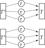
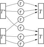
Figure S1: The two classes of Wick contractions for two-baryon correlators, represented as diagrams of tensor contractions involving perambulators $\tau$ and mode triplets $T$. Note that contractions involving spin indices are not indicated.

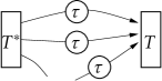
Figure S2: Source-sink partially contracted block.

The Wick contractions of quark fields yield two topologically distinct classes of diagrams, shown in Fig. S1. One possible strategy would be, in an intermediate step, to construct two-baryon “source” and “sink” tensors, where the former is the outer product of two mode triplets and the latter additionally includes the six perambulators. This would fully factorize the choice of source and sink operators in the correlator matrix. However, the computational cost would scale with $N_{\text{LapH}}^{6}$. Instead, we form partially-contracted source-sink “blocks” (Fig. S2) at a cost proportional to $N_{\text{LapH}}^{4}$. Computationally, this is the most costly step in the contractions, and therefore we avoid recomputing blocks that are used in multiple correlators. The cost of combining two blocks to complete a two-baryon contraction is proportional to $N_{\text{LapH}}^{2}$ and is relatively inexpensive. A similar strategy for two-baryon correlators was described recently in Ref. Hörz and Hanlon (2019).

In larger volumes, the $N_{\text{LapH}}^{4}$ cost scaling will eventually become prohibitively expensive. One possible solution is to use stochastic distillation Morningstar et al. (2011); Hörz et al. (2021), which would replace $N_{\text{LapH}}$ in the cost scaling with the (much smaller) size of the dilution space.

III.1 Choosing $N_{\text{LapH}}$

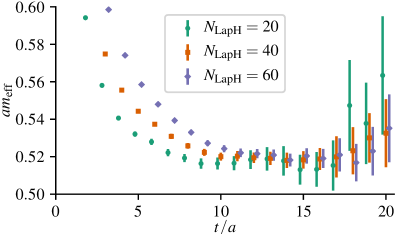
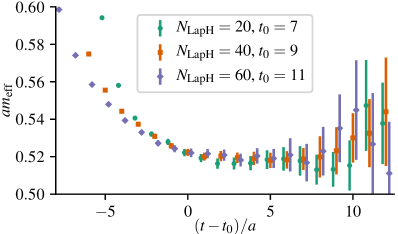
Figure S3: Left: Effective energies for an octet baryon correlator on U103 with $N_{\text{LapH}}=20,40,60$. Right: The effective energies shifted such that their plateaux start at $t-t_{0}=0$.

Due to the rise in inversion and contraction costs as $N_{\text{LapH}}$ is increased, it is computationally advantageous to use as few LapH eigenvectors as possible. However, making $N_{\text{LapH}}$ too small will increase the statistical uncertainty. Hence, for comparison, we computed an octet-baryon correlation function using three values of $N_{\text{LapH}}$ on a subset of ensemble U103. The effective energies are shown in the left panel of Fig. S3. It is clearly seen that the error on the effective energy increases as the number of LapH eigenvectors is reduced. At the same time, retaining fewer LapH eigenmodes has resulted in less contamination from the excited states; therefore, a more fair comparison between the three is one in which the onset of the plateau for each effective energy has been shifted to the same point. This is shown in the right panel of Fig. S3, indicating that $N_{\text{LapH}}=20$ is an acceptable choice. For the other $N_{f}=3$ ensembles, $N_{\text{LapH}}$ is scaled with the physical three-volume to ensure that the smearing radius remain roughly constant. For the $N_{f}=2$ ensembles, we have a single volume and we choose to use a slightly larger $N_{\text{LapH}}$, corresponding to a smaller smearing radius.

IV Analysis of correlation functions

The correlation functions computed are of the form

$$C_{ij}(t)\equiv\frac{1}{N_{t}}\sum_{\left\{t_{0}\right\}}\langle\mathcal{O}_{i}(t+t_{0})\mathcal{O}_{j}^{\dagger}(t_{0})\rangle,$$ (S29)

where $\left\{\mathcal{O}_{i}\right\}$ denotes a set of interpolating operators that all transform irreducibly in the same way, and $\left\{t_{0}\right\}$ is the set of $N_{t}$ sources shown in Fig. S4 for all ensembles. The sources and time separations that we include assume $t\ll T$ for periodic boundary conditions, and both $0\ll t_{0}$ and $t+t_{0}\ll T$ for open boundary conditions, such that the effects of the finite temporal extent may be ignored. Under these assumptions, the spectral decomposition of the correlators is given by

$$C_{ij}(t)=\sum_{n=0}^{\infty}\langle\Omega|\mathcal{O}_{i}|n\rangle\langle\Omega|\mathcal{O}_{j}|n\rangle^{\ast}e^{-E_{n}t},$$ (S30)

where $|\Omega\rangle$ is the vaccuum state, $|n\rangle$ are the eigenstates of the system, and $E_{n}$ are the eigenenergies.

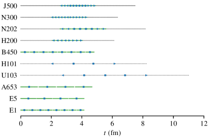
Figure S4: Location of source times on all ensembles. Triangles indicate sources used for only forward-propgating or backward-propagating states, and squares indicate sources used for both. When present, green line segments indicate the range over which sources were randomly shifted on each gauge configuration.

IV.1 Octet-baryon mass

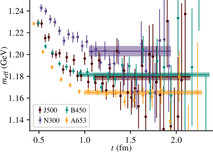
Figure S5: Effective energy for the octet baryon with total momentum zero on four ensembles with similar volumes. The bands show the value of the octet-baryon mass obtained from single-exponential fits to a single-octet-baryon correlator projected to zero momentum and also indicate the range of $t$ used for the fit.

In order to calculate $p^{2}$, which is needed for the phase-shift analysis, we must obtain an estimate for the octet-baryon mass. To this end, we perform single-exponential fits to correlators constructed from a single-octet-baryon operator projected to zero momentum. We show the resulting fits and effective energies on four ensembles with similar volumes in Fig. S5.

IV.2 Generalized eigenvalue problem

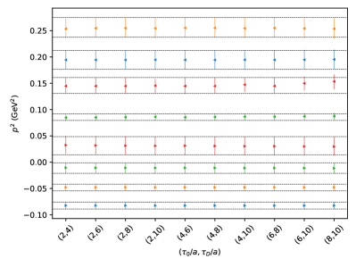
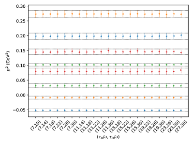
Figure S6: The center-of-mass scattering momentum $p^{2}$ versus the GEVP parameters $(\tau_{0},\tau_{D})$ for A653 (left) and J500 (right). The momentum frames include $\vec{P}L/(2\pi)=(0,0,0)$ (blue), $(0,0,1)$ (orange), $(0,1,1)$ (green), and $(1,1,1)$ (red). The ground states are denoted with right-facing triangles and the excited states with left-facing triangles. The second excited state in the rest frame and the spin-one states are not included. The dashed black lines show the upper and lower errors for each energy from the chosen values of $(\tau_{0}/a,\tau_{D}/a)$, which are $(4,8)$ for A653 and $(11,22)$ for J500.

For all momentum frames that include more than one two-baryon operator, we use the variational approach described in Refs. Lüscher and Wolff (1990); Blossier et al. (2009), in which a generalized eigenvalue problem (GEVP) is solved from the matrix of correlation functions in Eq. (S29):

$$C(t)\upsilon_{n}(t,\tau_{0})=\lambda_{n}(t,\tau_{0})C(\tau_{0})\upsilon_{n}(t,\tau_{0}).$$ (S31)

Provided that $\tau_{0}$ satisfies $\tau_{0}\geq t/2$, the asymptotic behavior of the generalized eigenvalues is given by Blossier et al. (2009)

$$\lambda_{n}(t)=|A_{n}|^{2}e^{-E_{n}t}\left[1+O(e^{-(E_{N}-E_{n})t})\right],$$ (S32)

where $N$ is the size of the correlator matrix, and the argument $\tau_{0}$ has been dropped. By contrast, the leading corrections to the eigenvalues of $C(t)$ only fall off as $e^{-t\Delta_{n}}$, where $\Delta_{n}\equiv\min_{m\neq n}|E_{n}-E_{m}|$. Thus, by solving the GEVP rather than the simple eigenvalue problem for $C(t)$, one benefits from a stronger suppression of the contamination from higher excitations.

To simplify the analysis, we turn the GEVP into a normal eigenvalue problem, resulting in the following matrix to be diagonalized

$$\hat{C}(t)\equiv C^{-1/2}(\tau_{0})C(t)C^{-1/2}(\tau_{0}),$$ (S33)

and only solve for the eigenvectors and eigenvalues at a single time separation $\tau_{D}>\tau_{0}$. The resulting eigenvectors can be used to rotate $\hat{C}(t)$ for all other time separations

$$\tilde{C}(t)\equiv V^{\dagger}(\tau_{D})C^{-1/2}(\tau_{0})C(t)C^{-1/2}(\tau_{0})V(\tau_{D}),$$ (S34)

where the columns of $V(\tau_{D})$ contain the orthonormal eigenvectors of $\hat{C}(\tau_{D})$. Then the diagonal elements of $\tilde{C}(t)$ approximate the generalized eigenvalues $\lambda_{n}(t)$. It can be seen in Fig. S6 that the scattering momenta derived from the spectrum show very little dependence on the chosen GEVP parameters $\tau_{0}$ and $\tau_{D}$. The rotated correlators are inspected by eye to ensure they remain statistically diagonal for all time separations.

Finally, extraction of the leading exponential terms for the diagonal elements of $\tilde{C}(t)$ gives the lowest $N$ levels that overlap with the states created by the operators used in the correlation matrix, and the overlaps themselves are given by

$$Z_{j}^{(n)}\equiv\bra{0}\mathcal{O}_{j}\ket{n}\approx C_{jk}^{1/2}(\tau_{0})V_{kn}(\tau_{D})A_{n}.$$ (S35)

These overlaps are used to identify states as being predominantly spin-zero or spin-one.

IV.3 Ratio fits

In a final step before fitting the correlators, we form a ratio of each diagonal element of the rotated correlator matrix to the product of two single-baryon correlators,

$$R_{n}(t)\equiv\frac{\tilde{C}_{nn}(t)}{C_{\Lambda}^{\vec{p}_{1}}(t)C_{\Lambda}^{\vec{p}_{2}}(t)}.$$ (S36)

The momenta $\vec{p}_{1,2}$ are chosen to correspond to the constituent momenta of the individual baryons appearing in the operator that has dominant overlap with state $n$. The advantage of forming this ratio is the possibility for partial cancellation of correlations and residual contributions from excited states. One drawback, however, is the loss of the monotonic behavior of the effective energy, making an identification of the plateau less reliable. To avoid this issue, in most cases we fix the lower end of the fit range, $t_{\rm min}$, on each ensemble to the first time separation in the plateau region of the single-baryon correlators, which were observed to take longer to reach their asymptotic behavior than the two-baryon correlators.

However, as mentioned in the main text, in some cases this choice of $t_{\rm min}$ corresponds to a poor signal quality in $R_{n}(t)$ and we instead chose a slightly lower $t_{\rm min}$. For all of these levels that are also used in the phase shift analysis, the decrease of $t_{\rm min}$ below the start of the single-baryon plateau was by less than 0.12 fm, except on ensemble N300 where the decrease was by 0.25 fm. These choices still lie in the plateau region of $R_{n}(t)$.

To estimate the systematic error corresponding to the chosen fit range, we extracted an alternative spectrum, based on a second value of $t_{\rm min}$ that is below our preferred value by somewhere between 0.0865–0.173 fm, and propagated it through to the subsequent analysis. Finally, the upper end of the fit range, $t_{\rm max}$, is chosen for each correlator ratio to be one time separation smaller than the first time separation in which $|R_{n}(t)|<3\;\text{error}(R_{n}(t))$. Effective energy differences for two additional ground-state levels are shown in Fig. S7.

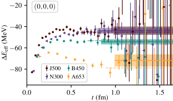
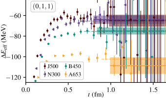
Figure S7: Effective energy differences for the ground state in frames $(0,0,0)$ (left) and $(0,1,1)$ (right) on four ensembles with similar volumes. See the caption of Fig. 2.

By fitting the ratio $R_{n}(t)$, one obtains the shift $\Delta E$ of the $n$th interacting energy eigenstate relative to the corresponding noninteracting level. The interacting energy $E$ is then reconstructed from $\Delta E$ by adding the noninteracting energy level, $\sqrt{p_{1}^{2}+m_{B}^{2}}+\sqrt{p_{2}^{2}+m_{B}^{2}}$, determined from the continuum dispersion relation using the single-octet-baryon energy at rest.

V Combined fits

We begin by describing the selection of levels that are included in the combined fits. In general, an energy level is excluded for one of four reasons:

1. Energy levels with dominant coupling to spin-one interpolating operators are excluded. The corresponding partial waves such as ${}^{3}P_{1}$ factorize in the quantization condition.

2. The spin-zero excited state in frames $(0,1,1)$ and $(1,1,1)$ cannot be described using the simplest form of the quantization condition. Assuming the phase shift does not pass through zero, Eq. (1) has a solution between the lowest pair of noninteracting levels, whereas the data lie below this range. Examining these levels in the nonrelativistic limit, one sees that they belong to the same degenerate shell of states, which can contain just one ${}^{1}S_{0}$ level. Therefore, higher partial waves are relevant. These levels can be described if ${}^{1}D_{2}$ is included in the quantization condition, which we leave to future work Green et al. ; they are excluded from all analyses here.

3. Energy levels with too-high $p^{2}$ are susceptible to the influence of the three-particle inelastic threshold, which is described by neither our fit ansatz nor the quantization condition. Therefore we exclude the second excited state in frame $(0,0,0)$ on all ensembles except for the two largest volumes, H101 and N202.

4. Energy levels with too-low $p^{2}$ are susceptible to the influence of the $t$-channel cut (arising from the exchange of a pseudoscalar meson), which is described by neither our fit ansatz nor the quantization condition. (We note that the method recently proposed in Ref. Meng and Epelbaum (2021) might be applicable.) However, on our coarser ensembles the bound-state pole also lies close to the $t$-channel cut. The ground state in frame $(0,0,1)$ is essential for constraining the pole position, and therefore we always include it, even though on our coarsest lattice spacing this level lies below the cut.

   On the other hand, for almost all ensembles the ground states in frames $(0,0,0)$ and $(0,0,2)$ lie below the cut and we exclude these levels. The exception is the largest volume, N202. However, these two levels still lie well below the bound-state pole and are very close to the cut; furthermore, we obtain significantly worse fit quality when either of these two levels is included. (For instance, the single-ensemble fit to the low-$p^{2}$ region of N202 has $\chi^{2}/\text{dof}=1.7/1$. Including the ground state in the rest frame increases this to 12.0/2. For the fit to the full-$p^{2}$ range, $\chi^{2}/\text{dof}$ increases from 4.1/3 to 8.2/4 when including this level.) Therefore, we also exclude these two levels on N202.

Our final choice of levels for the full $p^{2}$ range is the following: one or two excited-state levels in frame $(0,0,0)$, both the ground and excited spin-zero levels in frame $(0,0,1)$, and the ground state in frames $(0,1,1)$ and $(1,1,1)$. For the near-threshold region, we take the ground state in frame $(0,0,1)$ and possibly the ground state in frames $(0,1,1)$ and $(1,1,1)$.

The fits are performed by minimizing

$$\chi^{2}\equiv\sum_{i,j}(p^{2}_{i}-p^{2}_{\text{q.c.},i})\Sigma^{-1}_{ij}(p^{2}_{j}-p^{2}_{\text{q.c.},j})$$ (S37)

with respect to the model parameters, where $i$ indexes all of the levels among all ensembles included in the fit and $p^{2}_{\text{q.c.},i}$ is obtained by solving Eq. (1) given the model for $p\cot\delta(p)$. Here $\Sigma=\Sigma_{\text{stat}}+\Sigma_{\text{syst}}$ is an estimate of the covariance matrix. Bootstrap resampling is used to obtain $\Sigma_{\text{stat},ij}$, which is set to zero when $i$ and $j$ correspond to levels from different ensembles. The alternative spectrum fit range is used to estimate a correlated systematic uncertainty: we set $\Sigma_{\text{syst},ij}=(\delta p^{2})_{i}(\delta p^{2})_{j}$, where $\delta p^{2}$ is the the difference between $p^{2}$ obtained using the preferred and alternative spectra.

The statistical uncertainty of our fit results is estimated using bootstrap. When fitting to the near-threshold region, for a small number of bootstrap resamples (up to 4 out of 1000) the minimum of $\chi^{2}$ is not a point where its gradient vanishes, but instead lies at a discontinuity. In these rare cases, there exists a level (typically the lowest-lying level in the smallest volume) where the left-hand and right-hand sides of Eq. (1) are tangent and a small adjustment of the model parameters causes the solution to disappear. Although this represents a breakdown of the quantization condition and/or unphysical model parameters, we still keep these solutions in our statistical analysis as their effect is negligible. In addition to the bootstrap resamples, we also perform an additional fit using the alternative spectrum and take the difference in fit results as an estimate of systematic uncertainty.

A similar problem occurs for the bootstrap estimate of the uncertainty of the interacting spectrum in the continuum obtained using Eq. (1) and shown in Fig. 3. When $L$ is small, for some of the samples the ground state solution in frames $(0,0,0)$ and $(0,0,2)$ disappears. Because of this, we do not show an error band for these cases, which correspond roughly to energies below the $t$-channel cut.

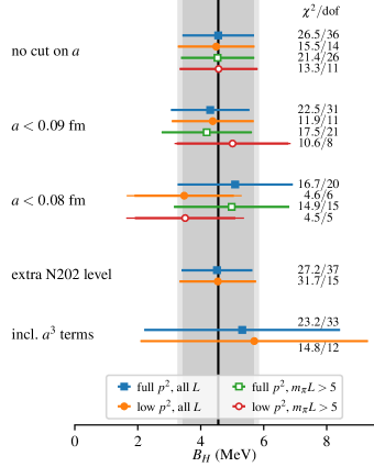
Figure S8: Binding energy, $\chi^{2}$, and number of degrees of freedom for various combined fits. The thin outer error bar includes the (usually negligible) estimate of systematic uncertainty based on the alternative spectrum, added in quadrature. Fits to the full $p^{2}$ range are indicated by squares and those to the near-threshold region by circles. Open symbols correspond to fits that exclude the two ensembles with $L\approx 2.1$ fm. The first three groupings exclude the zero, one, and two coarsest lattice spacings. The last two groupings are variations on the fits that include all ensembles, either adding the rest-frame ground state from N202 or parametrizing the fit coefficients as $c_{i}=c_{i0}+c_{i1}a^{2}+c_{i2}a^{3}$. The vertical line with inner and outer error bands show our final estimate, Eq. (5).

To estimate additional systematic uncertainty due to the continuum extrapolation and residual finite-volume effects, we apply various cuts to the selection of ensembles. In addition, to probe the ansatz for $p\cot\delta$, we use both a quadratic polynomial in $p^{2}$ with the full $p^{2}$ range and a linear polynomial with the near-threshold region. These fits are summarized in the first three groupings of Fig. S8. When fitting to all six lattice spacings, the resulting binding energy is very stable with respect to the inclusion of the small volumes and the choice of $p^{2}$ range. As the coarser lattice spacings are excluded, the variations increase, with the choice of $p^{2}$ range becoming more important than the cut on $L$. Our preferred fit, which provides our central value and statistical uncertainty, is the one that includes the most data, i.e. the first in the figure. We estimate the systematic uncertainty as the root-mean-square difference from the preferred fit of the central values of the seven other fits in the first and third groupings.

Figure S8 also shows two additional variations. Including the ground state in the rest frame from N202 has a negligible impact on the binding energy but can substantially increase $\chi^{2}$. Including $a^{3}$ terms in the dependence on the lattice spacing significantly increases the uncertainty, without improving the fit quality.

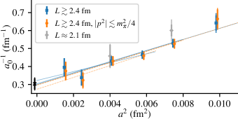
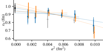
Figure S9: Inverse scattering length versus squared lattice spacing (top) and effective range versus squared lattice spacing (bottom). See the caption of Fig. 1.

The curves showing the dependence of $B_{H}$ on $a^{2}$ in Fig. 1 are based on the fits whose results are shown as filled blue squares and orange circles in the first three groupings of Fig. S8. The same is shown for $a_{0}^{-1}$ and $r_{0}$ in Fig. S9. The inverse scattering length shows a strong dependence on the lattice spacing (varying by a factor of two) and is fairly insensitive to the choice of $p^{2}$ range. The effective range has a weaker dependence on the lattice spacing but shows larger variation with the choice of $p^{2}$ range; this contributes to its relatively larger systematic uncertainty.

VI Two-flavor ensembles

In addition to our main analysis of $N_{f}=3$ lattice ensembles, we have generated new data for two $N_{f}=2$ ensembles (i.e. with dynamical $u$ and $d$ quarks and a quenched $s$ quark) used in our previous study of the $H$ dibaryon Francis et al. (2019) and listed in the lower part of Table SI. Based on the analysis in Ref. Draper and Sharpe (2021), we expect that the quenched $s$ quark is not an obstacle to using finite-volume quantization conditions. On both ensembles we elected to set the strange quark mass equal to that of the light quarks; this means that both ensembles have SU(3) flavor symmetry in the valence sector. For ensemble E5 with a pion mass of 437 MeV, this is a change from Ref. Francis et al. (2019) where we tuned the strange quark mass to be near its physical value; as a result, the main difference between E5 and the $N_{f}=3$ ensembles is that the strange quark is quenched.

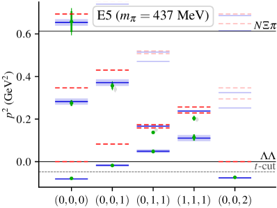
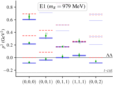
Figure S10: Two-baryon spectrum in five different reference frames on ensembles E5 (left) and E1 (right). Green points are the spin-zero levels and gray points are the spin-one levels. Horizontal lines indicate two- and three-particle thresholds and the $t$-channel cut. Horizontal line segments show finite-volume energies in the noninteracting case (dashed red) and from the fit to the wider $p^{2}$ range (solid blue).

Our analysis on the $N_{f}=2$ ensembles is the same as what was done in the $N_{f}=3$ case, except that we cannot study the continuum limit. The finite-volume spectra obtained from ensemble E5 are shown in the left panel of Fig. S10; they have the same qualitative features as observed for the $N_{f}=3$ ensembles. Performing fits of the phase shift, we obtain a binding energy

$$B_{H}=12.0\pm 2.7\pm 0.5\text{ MeV}\quad\text{(E5)},$$ (S38)

which is consistent with the binding energies in the $N_{f}=3$ case at similar nonzero lattice spacing.

The right panel of Fig. S10 shows the finite-volume spectra for ensemble E1. As the pion mass is much larger, the $t$-channel cut and three-particle threshold are further away from the threshold and all of the obtained levels lie in the region where the two-particle quantization condition is applicable. On this ensemble, the uncertainty of both the spectrum and the fitted quantities are dominated by systematics. The phase shift fits yield

$$B_{H}=17.3\pm 4.0\pm 5.4\text{ MeV}\quad\text{(E1)},$$ (S39)

which is consistent with the value $19\pm 10$ MeV reported in our previous work Francis et al. (2019) but has a smaller error.

In Fig. 5 we compare our results for the binding energy $B_{H}$ for $N_{f}=3$ and $N_{f}=2$ with the estimates from HAL QCD Inoue et al. (2011, 2012) and NPLQCD Beane et al. (2011a, b, 2013). Our $N_{f}=2$ calculations at nonzero lattice spacing show a dependence on the pion mass compatible with that observed by HAL QCD, although they lack the precision necessary to make an unambiguous statement. Moreover, this plot underscores our observation that discretization effects in this quantity are sizeable.

VII Spectrum data

The spectra used in this work are available in HDF5 format The HDF Group (2021) in the file levels.h5. Each dataset contains the bootstrap samples for one or more energy levels in lattice units, with the ensemble, frame, and type of energy level specified by the dataset’s key. For example, the following correspond to ensemble N300 and frame $\vec{P}L/(2\pi)=(0,1,1)$:

/N300/P011/octet_baryon  Dataset {1001},
/N300/P011/spin_one      Dataset {1001, 2, 1},
/N300/P011/spin_zero     Dataset {1001, 2, 2}.

The first entry of the first dimension contains the average over the ensemble and the next 1000 are the bootstrap samples. For the two-baryon spectrum, the second dimension indexes the preferred and alternative values in the first and second entries, and the third dimension indexes the energy levels in ascending order. As should be evident from the names, the first of these three datasets contains the octet baryon energy with momentum $\vec{P}$, the second contains the two-baryon level identified as spin one, and the last contains both two-baryon-levels identified as spin zero.